Singular Pöschl-Teller II potentials and gravitating kinks

Abstract

We report a two-dimensional (2D) gravitating kink model, for which both the background field equations and the linear perturbation equation are exactly solvable. The background solution describes a sine-Gordon kink that interpolating between two asymptotic AdS₂ spaces, and can be regarded as a 2D thick brane world solution. The linear perturbation equation can be recasted into a Schrödinger-like equation with singular Pöschl-Teller II potentials. There is no tachyonic state in the spectrum, so the solution is stable against the linear perturbations. Besides, there can be $n=0,1,2,\cdots$ bounded vibrational modes around the kink. The number of these vibrational modes varies with model parameters.

1 Introduction

Supersymmetric quantum mechanics (SUSY QM) offers us not only algebraic methods for solving quantum mechanical problems, but also some general conclusions on the structure of the spectrum CooperKhareSukhatme1995 ; GangopadhyayaMallowRasinariu2017 . These methods and conclusions are frequently applied to analyze the linear stability of kink solutions of scalar field theories in both flat BoyaCasahorran1989 ; AndradeMarquesMenezes2020 ; ZhongLiu2014 ; ZhongGuoFuLiu2018 and curved spaces DeWolfeFreedmanGubserKarch2000 ; Giovannini2001a ; ZhongLiu2013 .

A key concept in SUSY QM is the superpotential $\mathcal{W}(x)$. Given an arbitrary superpotential, one can always define two partner Hamiltonian operators: $H_{\pm}=-\frac{d^{2}}{dx^{2}}+V_{\pm}(x)$ with $V_{\pm}(x)=\mathcal{W}^{2}\pm\frac{d\mathcal{W}}{dx}$. Both of the Hamiltonians can be factorized as products of a linear differential operator $\mathcal{A}\equiv\frac{d}{dx}+\mathcal{W}$ and its hermitian conjugate $\mathcal{A}^{\dagger}=-\frac{d}{dx}+\mathcal{W}$:

$$H_{+}=\mathcal{A}\mathcal{A}^{\dagger},\quad H_{-}=\mathcal{A}^{\dagger}\mathcal{A}.$$

Usually, if $V_{\pm}(x)$ are both smooth, the spectra of $H_{\pm}$ are non-negative, and except the ground state, the structures of the spectra are equivalent CooperKhareSukhatme1995 ; GangopadhyayaMallowRasinariu2017 . Further, if the partner potentials $V_{\pm}(x)$ are shape invariant, i.e., $V_{+}(x;a_{0})=V_{-}(x;a_{1})+F(a_{1})$, where $a_{0},a_{1}$ are two sets of constant parameters, and $F(a_{1})$ is a function of $a_{1}$, then the corresponding Schrödinger equations are exactly solvable Gendenshtein1983 ; DuttKhareSukhatme1988 ; BougieGangopadhyayaMallow2010 .

The so called Pöschl-Teller (PT) II potentials PoschlTeller1933 are a pair of partner potentials generated by the following superpotential CooperKhareSukhatme1995 ; GangopadhyayaMallowRasinariu2017 :

$$\mathcal{W}(x;l,m)=l\tanh{x}-m\coth x,\quad l>m,$$ (1)

where $l$ and $m$ are two real parameters. One can easily check that the partner potentials

$$V_{\textrm{PT},+}(x;l,m) = (l-m)^{2}-l(l-1)\operatorname{sech}^{2}(x)+m(m+1){\rm{csch}}^{2}(x)$$ (2)

$$V_{\textrm{PT},-}(x;l,m) = (l-m)^{2}-l(l+1)\operatorname{sech}^{2}(x)+m(m-1){\rm{csch}}^{2}(x)$$ (3)

are shape invariant: $V_{\textrm{PT},+}(x;l,m)=V_{\textrm{PT},-}(x;l-1,m+1)+(l-m)^{2}-(m-l+2)^{2}$, and therefore, are exactly solvable.

When parameter $m=0$, the PT II potentials are smooth and finite, as can be seen from their expressions:

$$V_{\textrm{PT},+}(x;l,0) = l^{2}-l(l-1){\rm{sech}}^{2}(x),$$ (4)

$$V_{\textrm{PT},-}(x;l,0) = l^{2}-l(l+1){\rm{sech}}^{2}(x).$$ (5)

This regular version of PT II potentials is frequently seen in equations for linear perturbations around many static solutions. For example, the linear perturbations around the sine-Gordon kink and the $\phi^{4}$ kink in flat space satisfy Schrödinger-like equations with $V_{\textrm{PT},-}(x;1,0)$ and $V_{\textrm{PT},-}(x;2,0)$, respectively DashenHasslacherNeveu1974 ; GoldstoneJackiw1975 ; Rajaraman1975 . The solvability of these potentials makes it possible to give some quantitative discussions on the quantization DashenHasslacherNeveu1974 ; GoldstoneJackiw1975 ; Rajaraman1975 ; Jackiw1977 ; BoyaCasahorran1989 ; Evslin2021 and dynamical collision phenomena of kinks Sugiyama1979 ; Moshir1981 ; CampbellSchonfeldWingate1983 ; AnninosOliveiraMatzner1991 ; DoreyMershRomanczukiewiczShnir2011 ; TakyiWeigel2016 ; AdamOlesRomanczukiewiczWereszczynski2019a ; MantonOlesRomanczukiewiczWereszczynski2021 , see Vachaspati2006 for a comprehensive review. Perturbation equations of some de Sitter thick branes Wang2002 ; AfonsoBazeiaLosano2006 ; LiuZhongYang2010 or black holes solutions FerrariMashhoon1984 ; FerrariMashhoon1984a ; MossNorman2002 ; CardosoLemos2003 ; MolinaGiugnoAbdallaSaa2004 ; Jing2004 ; MolinaNeves2012 are also closely related to the regular PT II potentials.

When $m\neq 0$, at least one of the partner potentials will become singular. These singularities may cause an explicit breaking of supersymmetry between $H_{\pm}$, and make their spectra different, even worse, bound states with negative eigenvalues can appear, see Ref. CasahorranNam1991 for discussions on the case with $m=1$. Although singular PT II potentials have been found in the perturbation equations of some black hole solutions DuWangSu2004 ; CardonaMolina2017 ; BhattacharjeeSarkarBhattacharyya2021 , it is still unclear if such potentials are linked to any kink solution.

In fact, singular potentials have been found in the linear perturbation equations of some gravitating kink solutions, such as those in Refs. Stoetzel1995 ; Zhong2021 ; ZhongLiLiu2021 ; FengZhong2022 , where the kinks are embedding in some asymptotic AdS₂ spaces, and can be regarded as two-dimensional thick brane world solutions. Thus, it would be a natural conjecture that in some gravitating kink models, the linear perturbations are described by singular PT II potentials. However, constructing such kink models is not easy. Because to write the linear perturbation equation of a gravitating kink into a Schrödinger-like equation, one usually needs to introduce at least a metric dependent coordinate transformation Zhong2021 . If the scalar field that generates the kink is a K-field, namely, scalar fields with non-minimal first-order derivative couplings Armendariz-PiconMukhanovSteinhardt2001 ; Armendariz-PiconDamourMukhanov1999 ; GarrigaMukhanov1999 , then another coordinate transformation is needed ZhongLiLiu2021 ; Zhong2021b . Usually, these coordinate transformations are rather complicated, it is impossible even to obtain the explicit expression of the Schrödinger-like equations (see Zhong2021 ; ZhongLiLiu2021 ; FengZhong2022 ), needless to say to solve them exactly.

In this work, we consider a 2D gravitating kink model with a scalar K-field. We show that under certain conditions, the coordinate transformation caused by the derivative coupling of the K-field inverses the one caused by the metric. In this case, we can explicitly write out the Schrödinger-like equation for the linear perturbation without introducing any coordinate transformation. Moreover, we show that for the sine-Gordon kink, the linear perturbations are described by a Schrödinger-like equation with $V_{\textrm{PT},+}(x;l,1)$, where the value of parameter $l$ depends on the value of gravitational coupling and the expectation value of the vacuum. By tuning the value of $l$, we would have an arbitrary number of discrete bound states in the spectrum. To the author’s knowledge, this is the first 2D gravitating kink solution that has exactly solvable linear perturbation equation. This solution might be useful for considering the quantization and collisions of gravitating kinks.

This work is organized as follows. In the next section, after a briefly description of our model, we show that the field equations have simple first-order formalism, from which analytical kink solutions can be easily constructed. In section 3, we first review the linear stability issue of 2D gravitating kink. Then, we derive the condition under which the linear perturbation equation can be explicitly expressed without introducing coordinate transformations. Then, we move to an exactly solvable case in section 4. We end our work with some concluding remarks.

2 The model and the first-order equations

Following ZhongLiLiu2021 , we consider a 2D gravitating K-field model with the following action:

$$S=\frac{1}{\kappa}\int d^{2}x\sqrt{-g}\left[-\frac{1}{2}\nabla^{\mu}\varphi\nabla_{\mu}\varphi+\varphi R+\kappa\mathcal{L}(\phi,X)\right],$$ (6)

where $\kappa>0$ is the gravitational coupling constant, $\varphi$ is the dilaton field which couples with the curvature scalar $R$, and $X\equiv-\frac{1}{2}\nabla^{\mu}\phi\nabla_{\mu}\phi$ is the kinetic term of the scalar matter field $\phi$. Note that the Lagrangian density of a K-field can always be written as a function of $\phi$ and $X$.

We will looking for static gravitating kink solutions with the following metric:

$$ds^{2}=-e^{2A(x)}dt^{2}+dx^{2},$$ (7)

where $A(x)$ is called the warp factor RandallSundrum1999 ; RandallSundrum1999a . With this metric, the dilaton equation reduces to a simple algebraic equation Stoetzel1995 ; Zhong2021 ; ZhongLiLiu2021 ; FengZhong2022 :

$$\varphi(x)=2A(x),$$ (8)

and the independent dynamical equations we need to solve are the Einstein equations:

$$-4\partial_{x}^{2}A = \kappa\mathcal{L}_{X}(\partial_{x}\phi)^{2},$$ (9)

$$4\partial_{x}^{2}A+2\left(\partial_{x}A\right)^{2} = \kappa\mathcal{L},$$ (10)

where $\mathcal{L}_{X}\equiv\frac{\partial\mathcal{L}}{\partial{X}}$. Depending on the form of $\mathcal{L}(\phi,X)$, there can be more unknown variables than independent equations, in this case, we need to impose some constraints.

For the canonical case $\mathcal{L}=\bar{\mathcal{L}}\equiv X-V(\phi)$, there are three unknown variables of the system: $A(x)$, $\phi(x)$ and $V(\phi)$. Thus, we have to impose a constraint equation. It is convenient to introduce a function $W(\phi)$, whose form can be chosen arbitrarily, and constrain the kinetic term of the scalar field via

$$X=-\frac{1}{2}W_{\phi}^{2},$$ (11)

or equivalently,

$$\partial_{x}\phi=W_{\phi}\equiv\frac{dW(\phi)}{d\phi}.$$ (12)

Under this constraint, eqs. (9) and (10) give Stoetzel1995 ; Zhong2021 ; FengZhong2022

$$\partial_{x}A = -\frac{1}{4}\kappa W,$$ (13)

$$V = \frac{1}{2}W_{\phi}^{2}-\frac{1}{8}\kappa W^{2}.$$ (14)

If $W(\phi)$ is properly chosen, one can derive exact gravitating kink solutions from the first-order equations (12)-(14), see refs. Stoetzel1995 ; Zhong2021 ; FengZhong2022 ; LimaAlmeida2022 for examples. Note that eq. (13) also indicates the following relation

$$A(\phi)=-\frac{1}{4}\kappa\int\frac{W}{W_{\phi}}d\phi,$$ (15)

which will be used later.

For noncanonical scalars, the Einstein equations usually do not have simple first-order formalism, an exception can be found in ZhongLiLiu2021 . In present work, we consider a K-field model with the following Lagrangian density AdamQueiruga2011 ; ZhongLiu2015 :

$$\mathcal{L}=U(\phi)(X+\frac{1}{2}W_{\phi}^{2})^{2}+X-V(\phi),$$ (16)

where $W(\phi)$ is the same function introduced in eq. (11). This model has one more unknown variable than the canonical model, i.e., $U(\phi)$. Thus, we need to impose two constraints. If we also constrain $X=-\frac{1}{2}W_{\phi}^{2}$, as in the canonical case, then the Einstein equations (9)-(10) take the same form as those of the canonical model, because

$$\mathcal{L}_{X}\big{|}_{X=-\frac{1}{2}W_{\phi}^{2}}=1=\bar{\mathcal{L}}_{X},$$ (17)

and

$$\left.\mathcal{L}\right|_{X=-\frac{1}{2}W_{\phi}^{2}}=X-V(\phi)=\bar{\mathcal{L}}.$$ (18)

Consequently, the first-order equations (12)-(14) can also be used to construct solutions of the K-field model of (16). We call (16) a twinlike model of the canonical model, see AndrewsLewandowskiTroddenWesley2010 ; AdamQueiruga2011 ; BazeiaDantasGomesLosanoEtAl2011 ; BazeiaMenezes2011 ; AdamQueiruga2012 ; BazeiaDantas2012 ; BazeiaLobMenezes2012 ; BazeiaLobaoLosanoMenezes2014 ; ZhongLiu2015 ; ZhongFuLiu2018 ; AdamVarela2020 ; DantasRodrigues2020 ; BazeiaLosanoMarquesMenezes2020 for details and more examples of twinlike models.

The results obtained so far are irrelevant of $U(\phi)$, which will become important as soon as the linear perturbation issue is considered.

3 Linear perturbations

The linear perturbation issue for solutions of action (6) with metric (7) has been discussed in ZhongLiLiu2021 ; Zhong2021b . In this section, we first review the main steps of ZhongLiLiu2021 , and then apply the results to the model of (16).

To start with, we introduce the conformal flat coordinates:

$$ds^{2}=e^{2A(r)}(-dt^{2}+dr^{2}),$$ (19)

where

$$r\equiv\int e^{-A(x)}dx.$$ (20)

For simplicity, we will use overdots and primes to denote the derivatives with respect to $t$ and $r$, respectively. Suppose that $\{\varphi(r),\phi(r),g_{\mu\nu}(r)\}$ describe an arbitrary static solution of the field equations, and $\{\delta\varphi(r,t),\delta\phi(r,t),\delta g_{\mu\nu}(r,t)\}$ are small perturbations around the solution, where

$$\delta g_{\mu\nu}(r,t) \equiv e^{2A(r)}h_{\mu\nu}(r,t)$$ (23)

$$= e^{2A(r)}\left(\begin{array}[]{cc}h_{00}(r,t)&\Phi(r,t)\\ \Phi(r,t)&h_{rr}(r,t)\\ \end{array}\right).$$

To fix the gauge degrees of freedom in the linear perturbation equations, we define a new variable $\Xi\equiv 2\dot{\Phi}-h_{00}^{\prime}$, and take $\delta\varphi=0$ as the gauge condition ZhongLiLiu2021 .

The linearization of the field equations leads to three independent equations. Two of them enable us to eliminate $\Xi$ and $h_{rr}$ in terms of $\delta\phi$, and the other, after eliminating $\Xi$ and $h_{rr}$, takes the following form ZhongLiLiu2021 :

$$-\ddot{\delta\phi}+\gamma\delta\phi^{\prime\prime}+\gamma\left(\frac{\gamma^{\prime}}{\gamma}+\frac{\mathcal{L}_{X}^{\prime}}{{\mathcal{L}_{X}}}\right)\delta\phi^{\prime}+\gamma\left[A^{\prime 2}-3A^{\prime\prime}+2\frac{A^{\prime\prime\prime}}{A^{\prime}}-2\left(\frac{A^{\prime\prime}}{A^{\prime}}\right)^{2}\right.$$

$$\left.-\frac{1}{2}\frac{\mathcal{L}_{X}^{\prime}}{\mathcal{L}_{X}}\frac{X^{\prime}}{X}-\frac{1}{2}\frac{X^{\prime\prime}}{X}+\frac{1}{4}\left(\frac{X^{\prime}}{X}\right)^{2}\right]\delta\phi+\gamma^{\prime}\left(\frac{A^{\prime\prime}}{A^{\prime}}-\frac{1}{2}\frac{X^{\prime}}{X}-A^{\prime}\right)\delta\phi=0,$$ (24)

where

$$\gamma\equiv 1+2\frac{\mathcal{L}_{XX}X}{\mathcal{L}_{X}},\quad\mathcal{L}_{XX}\equiv\frac{\partial^{2}\mathcal{L}}{\partial X^{2}}.$$ (25)

By rescaling the variable

$$G(r,t)\equiv\mathcal{L}_{X}^{1/2}\gamma^{1/4}\delta\phi(r,t),$$ (26)

and introducing another coordinate transformation $r\to y=\int dr\gamma^{-1/2}$, we obtain a compact wave equation ZhongLiLiu2021 :

$$-\partial_{t}^{2}G+\partial_{y}^{2}G-V_{\text{eff}}(y)G=0,$$ (27)

where

$$V_{\text{eff}}(y)\equiv\frac{\partial_{y}^{2}f}{f},$$ (28)

and

$$f(y)\equiv\mathcal{L}_{X}^{1/2}\gamma^{1/4}\frac{\partial_{y}\phi}{\partial_{y}A}.$$ (29)

Note that in order the rescaling (26) and the coordinate transformation $r\to y$ are meaningful, the scalar Lagrangian must satisfies the following conditions:

$$\mathcal{L}_{X}>0,\quad\gamma>0.$$ (30)

After conducting the modes expansion

$$G(y,t)=\sum_{n}e^{i\omega_{n}t}\psi_{n}(y),$$ (31)

eq. (27) becomes a Schrödinger-like equation of $\psi_{n}(y)$ ZhongLiLiu2021 :

$${H}\psi_{n}\equiv-\frac{d^{2}\psi_{n}}{dy^{2}}+V_{\text{eff}}(y)\psi_{n}=\omega_{n}^{2}\psi_{n}.$$ (32)

The above Hamiltonian operator can be factorized as follows ZhongLiLiu2021 :

$$H={\mathcal{A}}{\mathcal{A}}^{\dagger},$$ (33)

where

$${\mathcal{A}}=\frac{d}{dy}+\frac{\partial_{y}f}{f},\quad{\mathcal{A}}^{\dagger}=-\frac{d}{dy}+\frac{\partial_{y}f}{f}.$$ (34)

We see that the superpotential is $\mathcal{W}(x)=\frac{\partial_{y}f}{f}$.

As we said in the introduction, the factorization of a Hamiltonian operator usually ensures the semipositive definite of the eigenvalues, i.e., $\omega_{n}^{2}\geq 0$. In this case, we say the background kink solution is stable against the linear perturbations. But if $V_{\text{eff}}(y)$ is singular, the factorization of a Hamiltonian operator dose not necessarily indicate the stability of the solution. The meaning of this statement will become clear, if we can find a gravitating kink solution with exactly solvable linear perturbation equation. The problem is that even if we can easily construct exact kink solutions in the $x$-coordinates by using the first-order equations (12)-(14), the complicated coordinate transformations from $x\to r$ and $r\to y$ would make it difficult, in general, to obtain the explicit expression of the Schrödinger-like equation (32), needless to say to solve it.

We noticed that it is possible to construct K-field models, such that the transformation from $r\to y$ inverses the one from $x\to r$. This is a very interesting situation, where both the transformations from $x\to r$ and from $r\to y$ are non-trivial, but their combination is a trivial identity transformation:

$$\frac{dy}{dx}=e^{-A}\gamma^{-1/2}=1.$$ (35)

In this case, the Schrödinger-like equation (32) can be obtained directly in the $x$-coordinates:

$${H}\psi_{n}\equiv-\frac{d^{2}\psi_{n}}{dx^{2}}+V_{\text{eff}}(x)\psi_{n}=\omega_{n}^{2}\psi_{n},$$ (36)

with

$$V_{\text{eff}}(x)\equiv\frac{\partial_{x}^{2}f}{f},$$ (37)

and

$$f(x)\equiv\mathcal{L}_{X}^{1/2}\gamma^{1/4}\frac{\partial_{x}\phi}{\partial_{x}A}.$$ (38)

In fact, the K-field model in (16) can realize the above idea, if $U(\phi)$ is properly chosen. For this model

$$\gamma|_{X=-\frac{1}{2}W_{\phi}^{2}}=1-2U(\phi)W_{\phi}^{2},$$ (39)

so the condition in eq. (35) can be satisfied if

$$\gamma|_{X=-\frac{1}{2}W_{\phi}^{2}}=e^{-2A},$$ (40)

in other words,

$$U(\phi)=\frac{1}{2W_{\phi}^{2}}(1-e^{\frac{\kappa}{2}\int\frac{W}{W_{\phi}}d\phi}).$$ (41)

To obtain the last equation we used eq. (15).

The discussion so far is valid for arbitrary function $W(\phi)$. After specify the form of $W(\phi)$, the Lagrangian in (16) will be completely fixed, as $U(\phi)$ and $V(\phi)$ can be calculated from eq. (41) and eq. (14), respectively. The solutions of $\phi(x)$ and $A(x)$ will be obtained by solving eqs. (12)-(13). Then, by substituting the background solution into eq. (38) and using eqs. (17) and (40) we obtain

$$f|_{X=-\frac{1}{2}W_{\phi}^{2}}=e^{-A/2}\frac{\partial_{x}\phi}{\partial_{x}A},$$ (42)

with which the effective potential $V_{\text{eff}}(x)\equiv\frac{\partial_{x}^{2}f}{f}$ of the Schrödinger-like equation can be calculated. Now, let us turn to an explicit example.

4 Sine-Gordon kink and the PT II potentials

The sine-Gordon kink is a typical kink solution, which can be obtained by taking

$$W(\phi)=kv^{2}\sin\left(\frac{\phi}{v}\right),$$ (43)

for which $U(\phi)$ and $V(\phi)$ take the following form:

$$U(\phi) = -\frac{1}{2k^{2}v^{2}}\sec^{2}\left(\frac{\phi}{v}\right)\left[\cos^{-\frac{1}{2}\kappa v^{2}}\left(\frac{\phi}{v}\right)-1\right],$$ (44)

$$V(\phi) = \frac{1}{16}k^{2}v^{2}\left[\left(\kappa v^{2}+4\right)\cos\left(\frac{2\phi}{v}\right)-\kappa v^{2}+4\right].$$ (45)

The solution of eqs. (12)-(13) read

$$\phi(x) = v\arcsin(\tanh(kx)),$$ (46)

$$A(x) = -\frac{1}{4}\kappa v^{2}\log(\cosh(kx)).$$ (47)

Obviously, the parameters $k$ and $v$ describe the thickness of the kink and the expectation value of the vacua, respectively. This solution can be regarded as a 2D thick brane solution, as the metric is asymptotically AdS₂, see DzhunushalievFolomeevMinamitsuji2010 for comprehensive of thick brane models in 5D.

From eq. (42) we get

$$f(x)=-\frac{4\text{csch}(kx)\cosh^{\frac{\kappa v^{2}}{2}}(kx)}{\kappa v}.$$ (48)

After denoting $l\equiv\frac{\kappa v^{2}}{2}>0$, and taking $k=1$, we obtain the expression of the effective potential:

$$V_{\rm{eff}}(x)\equiv\frac{\partial_{x}^{2}f}{f}=(l-1)^{2}-l(l-1)\text{sech}^{2}(x)+2\text{csch}^{2}(x),$$ (49)

which is nothing but one of the Pöschl-Teller II potential $V_{\textrm{PT},+}(x;l,m)$ with $m=1$. The corresponding partner potential is

$$V_{\textrm{PT},-}(x;l,1)=(l-1)^{2}-l(l+1)\text{sech}^{2}(x).$$ (50)

In figure 1, we plotted the shapes of $V_{\textrm{PT},+}$ and $V_{\textrm{PT},-}$ for $m=1$ and $l=2,3,4.$ We see that $V_{\textrm{PT},+}(x;l,1)$ is always divergent at $x=0$, while $V_{\textrm{PT},-}(x;l,1)$ is smooth. Besides, $V_{\textrm{PT},+}(x;l,1)$ is positive everywhere, which means the background kink solution is stable for these parameters.

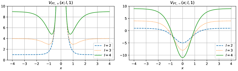
Figure 1: Plots of the effective potential $V_{\rm{eff}}(x)=V_{\textrm{PT},+}(x;l,1)$ and its partner potential $V_{\textrm{PT},-}(x;l,1)$ for $l=2,3,4$.

The properties of these two potentials have been discussed in ref. CasahorranNam1991 . For both potentials, the continuous spectrum starts from $(l-1)^{2}$. When the parameter $l$ is large enough, there can be some bound states for both potentials. The spectra of the bound states for $V_{\textrm{PT},+}(x;l,1)$ and $V_{\textrm{PT},-}(x;l,1)$ are CasahorranNam1991

$$E_{+,n}^{(l,1)}=(l-1)^{2}-(l-2n-3)^{2},\quad n=0,1,2,\cdots<\frac{l-3}{2},$$ (51)

and

$$E_{-,n}^{(l,1)}=(l-1)^{2}-(l-n)^{2},\quad n=0,1,2,\cdots<l,\quad l>1,$$ (52)

respectively. Here, instead of $\omega^{2}$, we used $E$ to represent the eigenvalues, just for simplicity. Obviously, the degeneracy between the spectra are only partly reserved: $E_{+,n}^{(l,1)}=E_{-,2n+3}^{(l,1)}$.

When $l>3$, $V_{\textrm{PT},+}(x;l,1)$ can capture bound states. For $l$ even or odd, $l=2p$ or $l=2p+1$ for some positive integer $p$, the number of bound states is $p-1$ CasahorranNam1991 . All the bound states of $V_{\textrm{PT},+}(x;l,1)$, when existing, have positive eigenvalues. Especially, the ground state has an eigenvalue $E_{+,0}^{(l,1)}=4l-8$. On the other hand, $V_{\textrm{PT},-}(x;l,1)$ always have a bound state with negative eigenvalue $E_{-,0}^{(l,1)}=1-2l$, and a zero mode $E_{-,1}^{(l,1)}=0$.

For example, when $l=4$, $V_{\textrm{PT},-}(x;4,1)$ has four bound states, the corresponding eigenvalues are $E_{-,n}^{(4,1)}=-7,0,5,8$, for $n=0,1,2,3$, respectively. While $V_{\textrm{PT},+}(x;4,1)$ only have one bound state with eigenvalue $E_{+,0}^{(4,1)}=8$. The corresponding wave function is

$$\psi_{+,0}^{(4,1)}(x)=\sqrt{\frac{5}{2}}\tanh^{2}(x)\text{sech}(x).$$ (53)

From eq. (31) we know that this bound state corresponds to a vibrational modes, with frequency $\omega_{0}=2\sqrt{2}$, around the kink. Note that the wave function $\psi_{+,0}^{(4,1)}(x)$ is vanished at $x=0$, see figure 2. This behavior of wave function is caused by the hard singularity of the effective potential. Here, by hard singularity, we mean a term $\sim\frac{\alpha}{x^{2}}$ with $\alpha\geq\frac{3}{4}$ FrankLandSpector1971 . One may check that when $x\to 0$ the singular PT II potentials $V_{\textrm{PT},+}(x;l,1)$ scaling as $\frac{2}{x^{2}}$. Therefore, $V_{\textrm{PT},+}(x;l,1)$ has a hard singularity at $x=0$, which will force $\psi_{+,n}^{l,1}(0)=0$, and the range of $x$ is effectively broken into two disjoint pieces $x<0$ and $x>0$ with no communication between them CooperKhareSukhatme1995 .

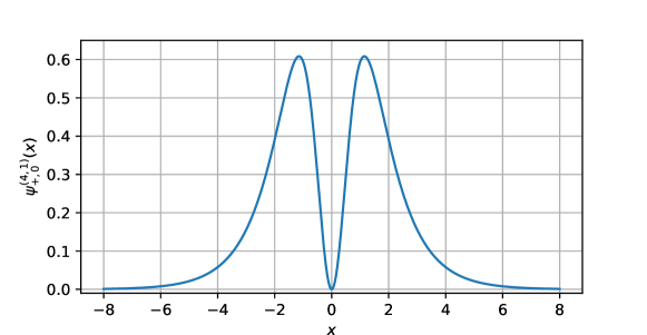
Figure 2: Wave function of the bound state of $V_{\rm{eff}}(x)=V_{\textrm{PT},+}(x;4,1)$.

5 Concluding remarks

In this work, we studied a special K-field model in a two-dimensional dilaton gravity theory. The Lagrangian density of the scalar K-field is carefully chosen such that the field equations take the same form as those of the canonical model, and the Schrödinger-like equation for the linear perturbation can be obtained without doing coordinate transformation. We found that when the background solution is a sine-Gordon kink, the linear perturbation equation becomes a Schrödinger-like equation with the exactly solvable PT II potentials $V_{\textrm{PT},+}(x;l,1)$, where the parameter $l$ depends on the gravitational coupling and the expectation value of the vacuum.

This potential is singular at $x=0$, which leads to some exotic properties. For example, although the Hamiltonians correspond to $V_{\textrm{PT},+}(x;l,1)$ and $V_{\textrm{PT},-}(x;l,1)$ are both factorizable, there is always a bound state of $V_{\textrm{PT},-}(x;l,1)$ with negative eigenvalues $E_{-,0}^{(l,1)}=1-2l$. The spectra of $V_{\textrm{PT},+}(x;l,1)$ and $V_{\textrm{PT},-}(x;l,1)$ are largely different, only parts of their states are degenerated. For asymmetric singular potentials, such as the Morse potentials, the spectra of the partner potentials will be completely different PanigrahiSukhatme1993 .

The bound state spectrum of $V_{\textrm{PT},+}(x;l,1)$ is $(l-1)^{2}-(l-2n-3)^{2}$, where $n=0,1,2,\cdots<\frac{l-3}{2}$. Thus, when $l>3$, $V_{\textrm{PT},+}(x;l,1)$ begins to capture bound states. Each of these bound states corresponds to a vibrational mode around the kink. We considered an explicit case with $l=4$, for which $V_{\textrm{PT},+}(x;4,1)$ has one bound state, whose wave function is vanished at $x=0$, as forced by the strong singularity of the potential. More bound states will appear as $l$ increases.

This exactly solvable model might be useful for studying the quantization and the collisions of gravitating kinks. The method of the present work can also be extended to other higher-dimensional scalar-gravity models. For example, one may try to constructing cosmic inflation or brane world models with exactly solvable linear perturbation equations by introducing K-fields. It is worth to mention that the perturbation issue of the present work corresponds to the scalar perturbation problems of higher-dimensional models. With these higher-dimensional models, one may ask what are the possible phenomenological implications of the hard singularity as well as the vibrational modes. We leave these issues for our future works.

References

- (1) F. Cooper, A. Khare and U. Sukhatme, Supersymmetry and quantum mechanics, Phys. Rep. 251 (1995) 267 [hep-th/9405029].
- (2) A. Gangopadhyaya, J. V. Mallow and C. Rasinariu, Supersymmetric Quantum Mechanics: An Introduction. World Scientific, 2017, 10.1142/10475.
- (3) L. J. Boya and J. Casahorran, General scalar bidimensional models including kinks, Annals Phys. 196 (1989) 361.
- (4) I. Andrade, M. A. Marques and R. Menezes, Stability of kinklike structures in generalized models, Nucl. Phys. B 951 (2020) 114883 [1906.05662].
- (5) Y. Zhong and Y.-X. Liu, -field kinks: stability, exact solutions and new features, J. High Energy Phys. 1410 (2014) 41 [1408.4511].
- (6) Y. Zhong, R.-Z. Guo, C.-E. Fu and Y.-X. Liu, Kinks in higher derivative scalar field theory, Phys. Lett. B 782 (2018) 346 [1804.02611].
- (7) O. DeWolfe, D. Z. Freedman, S. S. Gubser and A. Karch, Modeling the fifth dimension with scalars and gravity, Phys. Rev. D 62 (2000) 046008 [hep-th/9909134].
- (8) M. Giovannini, Gauge invariant fluctuations of scalar branes, Phys. Rev. D 64 (2001) 064023 [hep-th/0106041].
- (9) Y. Zhong and Y.-X. Liu, Linearization of thick K-branes, Phys. Rev. D 88 (2013) 024017 [1212.1871].
- (10) L. E. Gendenshtein, Derivation of Exact Spectra of the Schrodinger Equation by Means of Supersymmetry, JETP Lett. 38 (1983) 356.
- (11) R. Dutt, A. Khare and U. P. Sukhatme, Supersymmetry, Shape Invariance and Exactly Solvable Potentials, Am. J. Phys. 56 (1988) 163.
- (12) J. Bougie, A. Gangopadhyaya and J. V. Mallow, Generation of a Complete Set of Supersymmetric Shape Invariant Potentials from an Euler Equation, Phys. Rev. Lett. 105 (2010) 210402 [1008.2035].
- (13) G. Pöschl and E. Teller, Bemerkungen zur Quantenmechanik des anharmonischen Oszillators, Z. Phys. 83 (1933) 143.
- (14) R. F. Dashen, B. Hasslacher and A. Neveu, Nonperturbative methods and extended-hadron models in field theory. ii. two-dimensional models and extended hadrons, Phys. Rev. D 10 (1974) 4130.
- (15) J. Goldstone and R. Jackiw, Quantization of Nonlinear Waves, Phys. Rev. D 11 (1975) 1486.
- (16) R. Rajaraman, Some Nonperturbative Semiclassical Methods in Quantum Field Theory: A Pedagogical Review, Phys. Rept. 21 (1975) 227.
- (17) R. Jackiw, Quantum meaning of classical field theory, Rev. Mod. Phys. 49 (1977) 681.
- (18) J. Evslin, Evidence for the unbinding of the kink’s shape mode, JHEP 09 (2021) 009 [2104.14387].
- (19) T. Sugiyama, Kink-antikink collisions in the two-dimensional model, Prog. Theor. Phys. 61 (1979) 1550.
- (20) M. Moshir, Soliton - Anti-soliton Scattering and Capture in Theory, Nucl. Phys. B 185 (1981) 318.
- (21) D. K. Campbell, J. F. Schonfeld and C. A. Wingate, Resonance structure in kink-antikink interactions in theory, Physica D: Nonlinear Phenomena 9 (1983) 1.
- (22) P. Anninos, S. Oliveira and R. A. Matzner, Fractal structure in the scalar theory, Phys. Rev. D 44 (1991) 1147.
- (23) P. Dorey, K. Mersh, T. Romanczukiewicz and Y. Shnir, Kink-antikink collisions in the model, Phys. Rev. Lett. 107 (2011) 091602 [1101.5951].
- (24) I. Takyi and H. Weigel, Collective Coordinates in One-Dimensional Soliton Models Revisited, Phys. Rev. D 94 (2016) 085008 [1609.06833].
- (25) C. Adam, K. Oles, T. Romanczukiewicz and A. Wereszczynski, Spectral Walls in Soliton Collisions, Phys. Rev. Lett. 122 (2019) 241601 [1903.12100].
- (26) N. S. Manton, K. Oles, T. Romanczukiewicz and A. Wereszczynski, Collective Coordinate Model of Kink-Antikink Collisions in Theory, Phys. Rev. Lett. 127 (2021) 071601 [2106.05153].
- (27) T. Vachaspati, Kinks and domain walls. Cambridge University Press, 2006.
- (28) A. Wang, Thick de sitter brane worlds, dynamic black holes and localization of gravity, Phys. Rev. D 66 (2002) 024024 [hep-th/0201051].
- (29) V. I. Afonso, D. Bazeia and L. Losano, First-order formalism for bent brane, Phys. Lett. B 634 (2006) 526 [hep-th/0601069].
- (30) Y.-X. Liu, Y. Zhong and K. Yang, Scalar-kinetic branes, Europhys. Lett. 90 (2010) 51001 [0907.1952].
- (31) V. Ferrari and B. Mashhoon, New approach to the quasinormal modes of a black hole, Phys. Rev. D 30 (1984) 295.
- (32) V. Ferrari and B. Mashhoon, Oscillations of a Black Hole, Phys. Rev. Lett. 52 (1984) 1361.
- (33) I. G. Moss and J. P. Norman, Gravitational quasinormal modes for anti-de Sitter black holes, Class. Quant. Grav. 19 (2002) 2323 [gr-qc/0201016].
- (34) V. Cardoso and J. P. S. Lemos, Quasinormal modes of the near extremal Schwarzschild-de Sitter black hole, Phys. Rev. D 67 (2003) 084020 [gr-qc/0301078].
- (35) C. Molina, D. Giugno, E. Abdalla and A. Saa, Field propagation in de Sitter black holes, Phys. Rev. D 69 (2004) 104013 [gr-qc/0309079].
- (36) J.-L. Jing, Dirac quasinormal modes of the Reissner-Nordstrom de Sitter black hole, Phys. Rev. D 69 (2004) 084009 [gr-qc/0312079].
- (37) C. Molina and J. C. S. Neves, Wormholes in de Sitter branes, Phys. Rev. D 86 (2012) 024015 [1204.1291].
- (38) J. Casahorran and S. Nam, Singular superpotentials and explicit breaking of supersymmetry, Int. J. Mod. Phys. A 6 (1991) 2729.
- (39) D.-P. Du, B. Wang and R.-K. Su, Quasinormal modes in pure de Sitter space-times, Phys. Rev. D 70 (2004) 064024 [hep-th/0404047].
- (40) A. F. Cardona and C. Molina, Quasinormal modes of generalized Pöschl–Teller potentials, Class. Quant. Grav. 34 (2017) 245002 [1711.00479].
- (41) S. Bhattacharjee, S. Sarkar and A. Bhattacharyya, Scalar perturbations of black holes in Jackiw-Teitelboim gravity, Phys. Rev. D 103 (2021) 024008 [2011.08179].
- (42) B. Stötzel, Two-dimensional gravitation and Sine-Gordon solitons, Phys. Rev. D 52 (1995) 2192 [gr-qc/9501033].
- (43) Y. Zhong, Revisit on two-dimensional self-gravitating kinks: superpotential formalism and linear stability, JHEP 04 (2021) 118 [2101.10928].
- (44) Y. Zhong, F.-Y. Li and X.-D. Liu, K-field kinks in two-dimensional dilaton gravity, Phys. Lett. B 822 (2021) 136716 [2108.10166].
- (45) J. Feng and Y. Zhong, Scalar perturbation of gravitating double-kink solutions, 2202.02946.
- (46) C. Armendariz-Picon, V. F. Mukhanov and P. J. Steinhardt, Essentials of k essence, Phys. Rev. D 63 (2001) 103510 [astro-ph/0006373].
- (47) C. Armendariz-Picon, T. Damour and V. F. Mukhanov, k-inflation, Phys. Lett. B 458 (1999) 209 [hep-th/9904075].
- (48) J. Garriga and V. F. Mukhanov, Perturbations in -inflation, Phys. Lett. B 458 (1999) 219 [hep-th/9904176].
- (49) Y. Zhong, Normal modes for two-dimensional gravitating kinks, Phys. Lett. B 827 (2022) 136947 [2112.08683].
- (50) L. Randall and R. Sundrum, A large mass hierarchy from a small extra dimension, Phys. Rev. Lett. 83 (1999) 3370 [hep-ph/9905221].
- (51) L. Randall and R. Sundrum, An alternative to compactification, Phys. Rev. Lett. 83 (1999) 4690 [hep-th/9906064].
- (52) F. C. E. Lima and C. A. S. Almeida, Aspects of self-gravitating kink-like structures in 2D dilaton gravity, 2205.11570.
- (53) C. Adam and J. M. Queiruga, Algebraic construction of twinlike models, Phys. Rev. D 84 (2011) 105028 [1109.4159].
- (54) Y. Zhong and Y.-X. Liu, Matching the linear spectra of twinlike defects, Class. Quantum Grav. 32 (2015) 165002 [1408.6416].
- (55) M. Andrews, M. Lewandowski, M. Trodden and D. Wesley, Distinguishing -defects from their canonical twins, Phys. Rev. D 82 (2010) 105006 [1007.3438].
- (56) D. Bazeia, J. D. Dantas, A. R. Gomes, L. Losano and R. Menezes, Twinlike models in scalar field theories, Phys. Rev. D 84 (2011) 045010 [1105.5111].
- (57) D. Bazeia and R. Menezes, New results on twinlike models: Different field theories sharing the same extended solutions, Phys. Rev. D 84 (2011) 125018 [1111.1318].
- (58) C. Adam and J. M. Queiruga, Twinlike models with identical linear fluctuation spectra, Phys. Rev. D 85 (2012) 025019 [1112.0328].
- (59) D. Bazeia and J. D. Dantas, On the presence of twinlike models in cosmology, Phys. Rev. D 85 (2012) 067303 [1202.5978].
- (60) D. Bazeia, A. S. Lobão and R. Menezes, Twinlike models for kinks and compactons in flat and warped spacetime, Phys. Rev. D 86 (2012) 125021 [1210.6874].
- (61) D. Bazeia, A. S. Lobão, L. Losano and R. Menezes, First-order formalism for twinlike models with several real scalar fields, Eur. Phys. J. C 74 (2014) 2755 [1312.1198].
- (62) Y. Zhong, C.-E. Fu and Y.-X. Liu, Cosmological twinlike models with multi scalar fields, Sci. China Phys. Mech. Astron. 61 (2018) 90411 [1604.06857].
- (63) C. Adam and D. Varela, Inflationary twin models, Phys. Rev. D 101 (2020) 063514 [2003.05947].
- (64) J. D. Dantas and J. J. Rodrigues, Twinlike models for parametrized dark energy, Eur. Phys. J. C 80 (2020) 666 [2003.14351].
- (65) D. Bazeia, L. Losano, M. A. Marques and R. Menezes, New twinlike models for scalar fields, EPL 131 (2020) 31002 [2009.01613].
- (66) V. Dzhunushaliev, V. Folomeev and M. Minamitsuji, Thick brane solutions, Rept. Prog. Phys. 73 (2010) 066901 [0904.1775].
- (67) W. Frank, D. J. Land and R. M. Spector, Singular potentials, Rev. Mod. Phys. 43 (1971) 36.
- (68) P. K. Panigrahi and U. P. Sukhatme, Singular superpotentials in supersymmetric quantum mechanics, Phys. Lett. A 178 (1993) 251.