h KA-TP-22-2022
Leptonic Anomalous Magnetic and Electric Dipole Moments in the CP-violating NMSSM with and without Inverse Seesaw Mechanism

Abstract

The new results on the muon anomalous magnetic moment (AMM) published by Fermilab in 2021, did not lead to a reduction of its long-pending deviation from the Standard Model (SM) value by more than 4$\sigma$. The explanation of this discrepancy by adding new particles to the theory puts many new physics models under tension when combined with the null results of the LHC direct searches for new particles. In this paper, we investigate the CP-violating Next-to-Minimal Supersymmetric extension of the SM (NMSSM) with and without an inverse seesaw mechanism. We compute the one-loop supersymmetric contributions to the AMM and the two-loop Barr-Zee-type diagrams with effective Higgs couplings to photons for the leptonic electric dipole moments (EDMs). The effects of the extended (s)neutrino sector on the muon AMM and on the mass of the SM-like Higgs boson can be significant. Complex phases can have an important impact on the AMM. On the other hand, the stringent limits from the EDMs on the complex phases have to be taken into account. Our calculations have been implemented in the Fortran codes NMSSMCALC and NMSSMCALC-nuSS which are publicly available. Besides the leptonic AMMs and EDMs, these programs can compute the Higgs boson masses and mixings, together with Higgs boson decay widths and branching ratios taking into account the most up-to-date higher-order corrections in the NMSSM with and without inverse seesaw mechanism.

1 Introduction

At the beginning of 2021, the Fermilab Muon $g-2$ collaboration reported their first result [1] of the muon anomalous magnetic moment (AMM) $a_{\mu}\equiv(g_{\mu}-2)/2$,

$$a_{\mu}^{\text{FNAL}}=(11659204.0\pm 5.4)\times 10^{-10},$$ (1)

which is consistent with the previous measurement by the E821 experiment at BNL with [2]

$$a_{\mu}^{\text{BNL}}=(11659208.9\pm 6.3)\times 10^{-10}.$$ (2)

The combined result, $a_{\mu}^{\text{exp}}=(11659206.1\pm 4.1)\times 10^{-10}$ compared with the theoretical prediction of the Standard Model (SM) [3]

$$a_{\mu}^{\text{SM}}=(11659181.0\pm 4.3)\times 10^{-10}$$ (3)

leads to a deviation,

$$\Delta a_{\mu}\equiv a_{\mu}^{\text{exp}}-a_{\mu}^{\text{SM}}=(25.1\pm 5.9)\times 10^{-10},$$ (4)

at the $4.2\sigma$ level. The SM result consists of the pure QED, electroweak and hadronic contributions. The pure QED contribution has been evaluated up to ${\cal O}(\alpha^{5})$ [4] with negligible uncertainty, the electroweak correction has been computed up to leading three-loop order with less than one percent of uncertainty, see [3] and references therein, and is suppressed by the ratio $m_{\mu}^{2}/M_{W}^{2}$ where $m_{\mu}$ and $M_{W}$ are the mass of the muon and the $W$ boson, respectively. The largest uncertainty comes from the hadronic contributions which are calculated using non-pertubative methods. Very recently, the hadronic light-by-light contribution was computed by using lattice QCD [5] and slightly reduced the significance of the anomaly.

The anomaly is tantalizing in view of new physics at the weak scale [6]. Most of the models which try to explain this discrepancy tend to extend the electroweak sector to include additional corrections, $a_{\mu}^{\text{new}}$. In the Minimal Supersymmetric extension of the SM (MSSM), besides the two Higgs doublets $H_{u}$ and $H_{d}$, there are additional fields given by the superpartners of the muons, Higgs bosons and gauge bosons that interact directly with the muons. They enter the one-loop diagrams that contribute to $a_{\mu}^{\text{new}}$. The new contributions depend on the ratio $m_{\mu}^{2}/M_{S}^{2}$, where $M_{S}$ represents the mass scale of the supersymmetric (SUSY) particles and the muon Yukawa coupling $y_{\mu}=\sqrt{2}m_{\mu}/(v\cos\beta)$. Here $v$ denotes the vacuum expectation value given in terms of the two vacuum expectation values $v_{u}$ and $v_{d}$ of the two Higgs doublets $H_{u}$ and $H_{d}$, respectively, $v=\sqrt{v_{u}^{2}+v_{d}^{2}}$, and $\tan\beta\equiv v_{u}/v_{d}$. The new contribution $a_{\mu}^{\text{new}}$ can be significant when $M_{S}$ is small and/or $\tan\beta$ becomes large. The non-observation of SUSY particles at the LHC, however, pushes the SUSY mass scale $M_{S}$ to the TeV range. Moreover, the Higgs signals measured at the LHC require the SM-like Higgs couplings to be close to the ones of the SM, and therefore $\tan\beta$ should not be large. Furthermore, the SM-like Higgs should be the $h_{u}$-dominated Higgs boson so that it couples with a SM-like coupling to the top quarks. These requirements constrain the value of $a_{\mu}^{\text{new}}$.

The Next-to-Minimal Supersymmetric SM (NMSSM) contains an additional complex singlet superfield [7, 8, 9, 10, 11, 12, 13, 14, 15, 16, 17, 18, 19, 20, 21, 22]. Its scalar component can mix with the scalar components of the two Higgs doublet superfields which results in five neutral scalar Higgs boson states. Although the LHC Higgs data has pushed the mass of the dominantly doublet-like scalar/pseudoscalar Higgs states, $h_{d}/a_{d}$, into the TeV range it still allows for the singlet-like Higgs boson masses to be in the GeV range. This makes the NMSSM an interesting candidate for Higgs physics beyond the SM. As for the muon AMM, one expects a similar contribution from the electroweakino sector as in the MSSM. A noticeable difference may come from the contribution of a singlet-like Higgs boson with a mass of a few GeV. However, the one and two-loop light Higgs contributions are of opposite sign and therefore interfere destructively as shown in [23, 24]. When the (s)neutrino sector of the NMSSM is extended to include six singlet leptonic superfields ($\hat{N}_{i},\hat{X}_{i}$, $i=1,2,3$), the three very small neutrino masses can then be generated through the inverse seesaw mechanism [25, 26, 27]. This extension of the NMSSM was first discussed in [28]. The $h_{u}$-like Higgs boson now has interactions with the left-handed doublet neutrinos $\nu_{L}^{i}$ and the new singlet fermionic components $N^{i}$, and also with their scalar partners, that are proportional to the neutrino Yukawa couplings. These can induce new one-loop contributions to the Higgs boson masses as shown in [29, 30, 31]. This extension gives rise to the mixing between left-handed doublet sneutrinos $\tilde{\nu}_{L}^{i}$ with the right-handed ones so that the sneutrino masses can be rather light. This opens the possibility that the lightest sneutrinos can be a feasible Dark Matter candidate, as shown in [32, 33]. The extended sneutrino sector also gives rise to a new one-loop contribution to the AMM of the charged leptons, as shown in [34, 35].

In this study we compute and subsequently discuss the full one-loop SUSY contributions to the leptonic AMM and electric dipole moment (EDM) in the NMSSM and a variant of the NMSSM with inverse seesaw mechanism (abbreviated as NMSSM-nuSS) taking into account non-vanishing CP-violating phases. We further include contributions from the two-loop Barr-Zee-type diagrams with effective $h\gamma\gamma$ couplings. We show in this study the correlation between the impacts of the extended (s)neutrino sector on the muon AMM and on the loop-corrected $h_{u}$-like Higgs boson mass. The impacts can be significant simultaneously. In the regions where a positive SUSY contribution to the muon AMM is necessary to explain the anomaly, the one-loop contributions from the extended (s)neutrino sector to the $h_{u}$-like Higgs boson mass can become negative since the sneutrino contributions dominate over the neutrino contributions. We also study the effects of the complex phases on the muon AMM in both models. All these contributions to the AMM and to the EDM of the charged leptons have been implemented in our two published Fortran codes NMSSMCALC [36, 37, 38, 39, 40] and NMSSMCALC-nuSS [31] which compute the Higgs boson masses and mixings, together with Higgs boson decay widths and branching ratios taking into account the most up-to-date higher-order corrections. The codes can be downloaded from the url:

https://www.itp.kit.edu/~maggie/NMSSMCALC/

and

https://www.itp.kit.edu/~maggie/NMSSMCALC-nuSS/

The paper is organised as follows. Section 2 introduces the models and our notations. In Section 3 we present our computation and analytical expressions of the one-loop and two-loop contributions to the leptonic AMM and EDM. The set-up of the calculation and the numerical analysis are given in Sec. 4. We conclude in section 5.

2 The Complex NMSSM and the NMSSM with Inverse Seesaw Mechanism

The difference between the complex NMSSM and the complex NMSSM with inverse seesaw mechanism manifests itself mainly in the neutrino and sneutrino sectors. We start with a short description of the complex NMSSM to introduce the model parameters. We follow the same notation which has been used in our previous studies [37, 36, 38, 39, 40]. The complex NMSSM superpotential is given by ($i,j=1,2$)

$$\mathcal{W}_{\text{NMSSM}}=\epsilon_{ij}[y_{e}\hat{H}^{i}_{d}\hat{L}^{j}\hat{E}^{c}+y_{d}\hat{H}_{d}^{i}\hat{Q}^{j}\hat{D}^{c}-y_{u}\hat{H}^{i}_{u}\hat{Q}^{j}\hat{U}^{c}]-\epsilon_{ij}\lambda\hat{S}\hat{H}_{d}^{i}\hat{H}_{u}^{j}+\frac{1}{3}\kappa{\hat{S}}^{3}\;,$$ (5)

with the quark and leptonic superfields $\hat{Q}$, $\hat{U}$, $\hat{D}$, $\hat{L}$, $\hat{E}$, and the Higgs doublet superfields $\hat{H}_{d}$, $\hat{H}_{u}$ and the singlet superfield $\hat{S}$ and the totally antisymmetric tensor $\epsilon_{12}=\epsilon^{12}=1$. Charge conjugated fields are denoted by the superscript $c$. Color and generation indices have been suppressed for the sake of clarity. The Yukawa couplings $y_{u},\ y_{d}$ and $y_{e}$ are taken as diagonal 3$\times$3 matrices in the flavour space. The coupling parameters $\lambda$ and $\kappa$ are complex numbers in the CP-violating NMSSM. The soft SUSY-breaking Lagrangian reads

$$\mathcal{L}_{\rm soft,NMSSM}= -m_{H_{d}}^{2}H_{d}^{\dagger}H_{d}-m_{H_{u}}^{2}H_{u}^{\dagger}H_{u}-m_{\tilde{Q}}^{2}\tilde{Q}^{\dagger}\tilde{Q}-m_{\tilde{L}}^{2}\tilde{L}^{\dagger}\tilde{L}-m_{\tilde{u}_{R}}^{2}\tilde{u}_{R}^{*}\tilde{u}_{R}-m_{\tilde{d}_{R}}^{2}\tilde{d}_{R}^{*}\tilde{d}_{R}$$

$$-m_{\tilde{e}_{R}}^{2}\tilde{e}_{R}^{*}\tilde{e}_{R}-(\epsilon_{ij}[y_{e}A_{e}H_{d}^{i}\tilde{L}^{j}\tilde{e}_{R}^{*}+y_{d}A_{d}H_{d}^{i}\tilde{Q}^{j}\tilde{d}_{R}^{*}-y_{u}A_{u}H_{u}^{i}\tilde{Q}^{j}\tilde{u}_{R}^{*}]+\mathrm{h.c.})$$

$$-\frac{1}{2}(M_{1}\tilde{B}\tilde{B}+M_{2}\tilde{W}_{j}\tilde{W}_{j}+M_{3}\tilde{G}\tilde{G}+\mathrm{h.c.})$$ (6)

$$-m_{S}^{2}|S|^{2}+(\epsilon_{ij}\lambda A_{\lambda}SH_{d}^{i}H_{u}^{j}-\frac{1}{3}\kappa A_{\kappa}S^{3}+\mathrm{h.c.})\;.$$

The $H_{u,d}$ are two scalar Higgs doublets fields, $S$ a scalar singlet field, $\tilde{Q}$ scalar squark doublets, $\tilde{L}$ scalar slepton doublets, $\tilde{u}_{R}$ and $\tilde{d}_{R}$ scalar squark singlet fields, and $\tilde{e}_{R}$ a scalar slepton singlet field. The soft SUSY-breaking gaugino mass parameters $M_{k}$ ($k=1,2,3$) of the bino, wino and gluino fields $\tilde{B}$, $\tilde{W}_{l}$ ($l=1,2,3$) and $\tilde{G}$ as well as the soft SUSY-breaking trilinear couplings $A_{x}$ ($x=\lambda,\kappa,u,d,e$) are complex in the CP-violating NMSSM.

After electroweak symmetry breaking, the Higgs boson fields can be expanded around their vacuum expectation values (VEVs) $v_{u}$, $v_{d}$, and $v_{s}$, respectively,

$$H_{d}=\begin{pmatrix}\frac{v_{d}+h_{d}+ia_{d}}{\sqrt{2}}\\ h_{d}^{-}\end{pmatrix},\,\,H_{u}=e^{i\varphi_{u}}\begin{pmatrix}h_{u}^{+}\\ \frac{v_{u}+h_{u}+ia_{u}}{\sqrt{2}}\end{pmatrix},\,\,S=\frac{e^{i\varphi_{s}}}{\sqrt{2}}(v_{s}+h_{s}+ia_{s})\,,$$ (7)

with the CP-violating phases $\varphi_{u,s}$ and we obtain the tree-level spectrum of the Higgs sector. The relation to the SM VEV $v\approx 246.22$ GeV is given by

$$v^{2}=v_{u}^{2}+v_{d}^{2}$$ (8)

and we define the mixing angle $\tan\beta$ as

$$\tan\beta=\frac{v_{u}}{v_{d}}\;.$$ (9)

The effective $\mu$ parameter is given by

$$\mu_{\text{eff}}=\frac{\lambda v_{s}e^{i\varphi_{s}}}{\sqrt{2}}.$$ (10)

Besides the gauge bosons, quarks, charged leptons, and three left-handed neutrino fields as in the SM, we have an extended Higgs spectrum and new SUSY particles, in particular:

• The CP-even and CP-odd Higgs interaction states $(h_{d,u,s},a_{u,d,s})$ mix to form five CP indefinite Higgs mass eigenstates $h_{i}$ ($i=1,...,5$), with their masses per convention ordered as $m_{h_{1}}<m_{h_{2}}<m_{h_{3}}<m_{h_{4}}<m_{h_{5}}$, and one neutral Goldstone boson $G^{0}$. We use a two-fold rotation to rotate from the interaction to the mass eigenstates,

  $$(h_{d},h_{u},h_{s},a,a_{s},G^{0})^{T} = \mathcal{R}^{G}(\beta)\,(h_{d},h_{u},h_{s},a_{d},a_{u},a_{s})^{T},$$ (11)

  $$(h_{1},h_{2},h_{3},h_{4},h_{5},G^{0})^{T} = \mathcal{R}^{H}\,(h_{d},h_{u},h_{s},a,a_{s},G^{0})^{T},$$ (12)

  where the first rotation matrix $\mathcal{R}^{G}$ with one rotation angle $\beta$ singles out the neutral Goldstone boson and the second rotation matrix $\mathcal{R}^{H}$ rotates the five interaction states $(h_{d},h_{u},h_{s},a,a_{s})$ to the five mass eigenstates $(h_{1},h_{2},h_{3},h_{4},h_{5})$.

• The charged Higgs interaction states $h_{d}^{\pm},h_{u}^{\pm}$ constitute the charged Higgs bosons $H^{\pm}$ with mass $M_{H^{\pm}}$ and the charged Goldstone bosons $G^{\pm}$.

• The fermionic partners of the neutral Higgs bosons, the neutral higgsinos $\tilde{H}_{u}$, $\tilde{H}_{d}$ and the singlino $\tilde{S}$, mix with the neutral gauginos $\tilde{B}$ and $\tilde{W}^{3}$, resulting in five neutralinos denoted as $\tilde{\chi}^{0}_{i}$, $(i=1,...,5)$. The mass ordering of the $\tilde{\chi}^{0}_{i}$ is chosen as $m_{\tilde{\chi}^{0}_{1}}\leq...\leq m_{\tilde{\chi}^{0}_{5}}$ and the rotation matrix $N$ transforms the fields $(\tilde{B},\ \tilde{W}^{3},\ \tilde{H}_{d},\ \tilde{H}_{u},\tilde{S})^{T}$ into the mass eigenstates.

• The two chargino mass eigenstates,

  $$\tilde{\chi}_{i}^{+}=\left(\begin{array}[]{c}\tilde{\chi}_{L_{i}}^{+}\\[2.84544pt] \overline{\tilde{\chi}_{R_{i}}^{-}}\end{array}\right)\;,\quad i=1,2\;,$$ (15)

  are obtained from the rotation of the interaction states, given by the charged Higgsinos $\tilde{H}^{\pm}_{d}$, $\tilde{H}^{\pm}_{u}$ and the charged gauginos $\tilde{W}^{\pm}$, to the mass eigenstates. This is done by a bi-unitary transformation with the two $2\times 2$ unitary matrices $V^{\chi}$ and $U^{\chi}$,

  $$\tilde{\chi}_{L}^{+}=V^{\chi}(\tilde{W}^{+},\tilde{H}^{+}_{u})^{T},\ \ \ \tilde{\chi}_{R}^{-}=U^{\chi}(\tilde{W}^{-},\tilde{H}^{-}_{d})^{T}.$$ (16)

• The scalar partners of the left- and right-handed up-type quarks are denoted by $\tilde{u}_{L/R}^{i}$, of the down-type quarks by $\tilde{d}^{i}_{L/R}$, and of the charged leptons by $\tilde{l}^{i}_{L/R}$ ($i=1,2,3$). We do not include flavor mixing. Within each flavour the left- and right-handed scalar fermions with same electric charge mix and they are rotated to the mass eigenstates by a unitary matrix $U^{\tilde{f}}$.

• There are three scalar partners of the left-handed neutrinos, denoted as $\tilde{\nu}_{i}$ ($i=1,2,3$) with their masses given by

  $$m^{2}_{\tilde{\nu}_{i}}=\frac{1}{2}M_{Z}^{2}c_{2\beta}+m_{\tilde{L}_{i}}^{2}\;,$$ (17)

  where the short hand notation $c_{x}\equiv\cos(x),s_{x}\equiv\sin(x),t_{x}\equiv\tan(x)$ is used in this paper and the second term comes from the soft SUSY-breaking Lagrangian in Eq. (2).

The complex NMSSM with inverse seesaw mechanism is obtained from the complex NMSSM by including six gauge-singlet chiral superfields $\hat{N}_{i}$, $\hat{X}_{i}$ ($i=1,2,3$) that carry lepton number. We follow the same notation as in our previous investigation of the loop corrections to the neutral Higgs boson masses presented in [31]. The superpotential of the model reads ($i,j=1,2$)

$$\mathcal{W}_{\text{NMSSM-nuSS}}=\mathcal{W}_{\text{NMSSM}}-y_{\nu}\epsilon_{ij}\hat{H}_{u}^{i}\hat{L}^{j}\hat{N}^{c}+\lambda_{X}\hat{S}\hat{X}\hat{X}+\mu_{X}\hat{X}\hat{N}^{c}\,,$$ (18)

where the neutrino Yukawa coupling $y_{\nu}$ and the coupling $\lambda_{X}$ are $3\times 3$ complex matrices in general, and the superscript $c$ denotes the charge conjugation. The $3\times 3$ matrix $\mu_{X}$ is the only parameter with the dimension of mass in the superpotential so that it can be of the order of the SUSY-conserving mass scale and is naturally large. The soft SUSY-breaking NMSSM Lagrangian respecting the gauge symmetries and the global $\mathbb{Z}_{3}$ symmetry reads (the assignment of the $\mathbb{Z}_{3}$ charges is provided in [31])

$$\mathcal{L}_{\text{NMSSM-nuSS}}^{\text{soft}}= \mathcal{L}_{\text{NMSSM}}^{\text{soft}}+(\epsilon_{ab}y_{\nu}A_{\nu}H_{u}^{a}\tilde{L}^{b}\tilde{N}^{*}+\lambda_{X}A_{X}S\tilde{X}\tilde{X}+\mu_{X}B_{\mu_{X}}\tilde{X}\tilde{N}^{*}+h.c.)$$

$$-\tilde{m}^{2}_{X}\left|\tilde{X}\right|^{2}-\tilde{m}^{2}_{N}\left|\tilde{N}\right|^{2}\;,$$ (19)

which introduces the soft SUSY-breaking trilinear couplings $A_{\nu},A_{X}$, the soft SUSY-breaking masses $\tilde{m}_{X}^{2},\tilde{m}_{N}^{2}$, and the soft SUSY-breaking bilinear mass $B_{\mu_{X}}$.

In the neutral leptonic sector, the three left-handed neutrinos $\nu_{L_{i}}$ mix with the six leptonic component fields of the six singlet superfields $\hat{N}_{i}^{c},\hat{X}_{i}$, $i=1,2,3$, and the mass term in the Lagrangian reads

$${\cal L}_{\text{mass}}^{\nu}=-\frac{1}{2}\begin{pmatrix}\nu_{L}&N^{c}&X\end{pmatrix}M_{\text{ISS}}^{\nu}\begin{pmatrix}\nu_{L}\\ N^{c}\\ X\end{pmatrix},$$ (20)

where the mixing mass matrix is given by

$$M_{\text{ISS}}^{\nu}=\begin{pmatrix}0&M_{D}&0\\ M_{D}^{T}&0&\mu_{X}\\ 0&\mu_{X}^{T}&M_{X}\end{pmatrix},$$ (21)

where blocks $M_{D},\mu_{X}$ and $M_{X}$ are $3\times 3$ matrices with $\mu_{X}$ defined in Eq. (18) and

$$M_{D}=\frac{v_{u}e^{i\varphi_{u}}}{\sqrt{2}}y_{\nu},\quad M_{X}=\frac{v_{s}e^{i\varphi_{s}}}{\sqrt{2}}(\lambda_{X}+\lambda_{X}^{T})\;.$$ (22)

Diagonalizing the neutrino mass matrix with a unitary rotation matrix $U^{\nu}$, one obtains nine neutrino mass eigenstates with their masses $m_{\nu_{i}}$ $(i=1,...,9)$ being sorted in ascending order. By exploiting the fact that all matrix elements of $M_{D}$ and $M_{X}$ are much smaller than the eigenvalues of $\mu_{X}$, the $3\times 3$ light neutrino mass matrix can be expressed at leading order as

$$M_{\text{light}}=M_{D}M_{N}^{-1}M_{D}^{T}\,,\;\mbox{ with }\;M_{N}=\mu_{X}M_{X}^{-1}\mu_{X}^{T}\,,$$ (23)

and then can be diagonalized by the Pontecorvo-Maki-Nakagawa-Sakata (PMNS) matrix $U_{\text{PMNS}}$,

$$U_{\text{PMNS}}^{*}M_{\text{light}}U_{\text{PMNS}}^{\dagger}=m_{\nu}\;,\quad m_{\nu}=\text{diag}({m_{\nu_{1}}},{m_{\nu_{2}}},{m_{\nu_{3}}}).$$ (24)

In order to reproduce the light neutrino oscillation data, two different parameterizations have been considered. In the so-called Casas-Ibarra parameterization [41], $M_{D}$ is computed from the relation

$$M_{D}=U_{\text{PMNS}}^{T}\sqrt{m_{\nu}}R\sqrt{{{\mathcal{M}}}_{N}}V_{\nu},\quad{{\mathcal{M}}}_{N}=\text{diag}({M_{N_{1}}},{M_{N_{2}}},{M_{N_{3}}})=V^{*}_{\nu}M_{N}V^{\dagger}_{\nu}\;,$$ (25)

with $R$ being a complex orthogonal matrix and $V_{\nu}$ a unitary matrix diagonalizing $M_{N}$. The $y_{\nu}$ are then obtained from Eq. (22). The other possibility is to use the $\mu_{X}$-parameterization [42] in which $M_{X}$ is computed from the relation

$$M_{X}=\mu_{X}^{T}M_{D}^{-1}U_{\text{PMNS}}^{*}m_{\nu}U_{\text{PMNS}}^{\dagger}M_{D}^{T,-1}\mu_{X},$$ (26)

where $M_{D}$ is calculated from the input $y_{\nu}$.

In the sneutrino sector, each sneutrino field is split up into its CP-even and CP-odd components as

$${\tilde{\nu}} =\frac{1}{\sqrt{2}}\left({\tilde{\nu}}_{+}+i{\tilde{\nu}}_{-}\right),$$ (27)

$${\tilde{N}}^{*} =\frac{1}{\sqrt{2}}\left({\tilde{N}}_{+}+i{\tilde{N}}_{-}\right),$$ (28)

$${\tilde{X}} =\frac{1}{\sqrt{2}}\left({\tilde{X}}_{+}+i{\tilde{X}}_{-}\right).$$ (29)

The mass term in the basis $\psi=({\tilde{\nu}}_{+},{\tilde{N}}_{+},{\tilde{X}}_{+},{\tilde{\nu}}_{-},{\tilde{N}}_{-},{\tilde{X}}_{-})^{T}$ (generation indices are suppressed) is given by

$${\cal L}=\frac{1}{2}\psi^{T}M_{{\tilde{\nu}}}\psi\;,$$ (30)

where the mass matrix $M_{\tilde{\nu}}$ is an $18\times 18$ symmetric matrix that can be found in Appendix A. An orthogonal matrix ${U_{\tilde{\nu}}}$ can be used to obtain the masses of the sneutrinos as

$$\text{diag}\left(m^{2}_{\tilde{n}_{1}},\cdots,m^{2}_{\tilde{n}_{18}}\right)={U_{\tilde{\nu}}}M_{\tilde{\nu}}{U_{\tilde{\nu}}}^{T},$$ (31)

where their mass values are ordered as $m^{2}_{\tilde{n}_{1}}\leq\cdots\leq m^{2}_{\tilde{n}_{18}}$.

3 SUSY Contributions to the Leptonic AMM and EDM

The SUSY contributions to the leptonic AMM $a_{l}$ and EDM $d_{l}$ ($l=e,\mu,\tau$ ) can be calculated in perturbation theory by considering the matrix element decomposed into a relativistic covariant form,

$$\langle l(p_{2})|j^{\mu}(q)|l(p_{1})\rangle = -ie\bar{u}(p_{2})\bigg{[}\left(\gamma^{\mu}-\frac{\not{q}q^{\mu}}{q^{2}}\right)(\bar{F}_{L}(q^{2})P_{L}+\bar{F}_{L}^{*}(q^{2})P_{R})$$

$$+\frac{i\sigma^{\mu\nu}q_{\nu}}{2m_{l}}(F_{L}(q^{2})P_{L}+F_{L}^{*}(q^{2})P_{R})+\frac{q_{\mu}}{m_{l}}(\bar{\bar{F}}_{L}(q^{2})P_{L}+\bar{\bar{F}}_{L}^{*}(q^{2})P_{R})\bigg{]}u(p_{1})$$

where $\sigma^{\mu\nu}=\frac{i}{2}[\gamma^{\mu},\gamma^{\nu}]$, $P_{L/R}=\frac{1\mp\gamma_{5}}{2}$, $q=p_{2}-p_{1}$, $m_{l}$ is the lepton mass and $u(p)$ denotes the Dirac spinor. The form factors $F_{L}$, $\bar{F}_{L}$, $\bar{\bar{F}}_{L}$ are functions of $q^{2}$ and other parameters of the model. The operator $\sigma^{\mu\nu}q_{\nu}$ is called dipole matrix operator. In the static limit ($q^{\mu}\to 0$) we have [43]:

$$a_{l}=\text{Re}[F_{L}(0)],\quad d_{l}=\frac{e}{2m_{l}}\text{Im}[F_{L}(0)].$$ (33)

In our computation we will use this generic form for both the AMM and EDM keeping all possible complex phases.

3.1 One-Loop Contributions

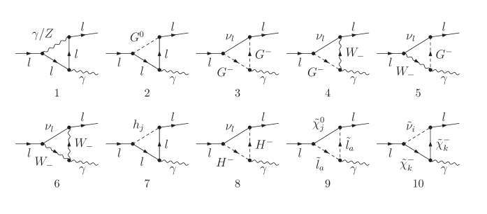
Figure 1: Generic one-loop Feynman diagrams contributing to the dipole matrix form factor.

It is well known that the contributions to the dipole matrix $\sigma^{\mu\nu}q_{\nu}$ require a chirality flip. Therefore contributions to $F_{L}(0)$ are proportional either to the mass of the external lepton or to the masses of the fermions running in the loop diagrams. In Fig. 1, we present all one-loop diagrams which contribute to $F_{L}(0)$ in the NMSSM-nuSS. Diagrams with neutral or charged Goldstone bosons occur explicitly because we work in the Feynman-’t Hooft gauge. The diagrams 1 and 2 are the same as in the SM. The diagram with the photon exchange belongs to the QED contribution and the diagrams with $Z$ and $G^{0}$ belong to the weak contribution. We calculated these diagrams and recovered the results quoted in the literature, see for example [43] and references therein. Since we donot account them in $a_{l}^{\text{new}}$ we do not present their explicit expressions here and will not mention them any more. The diagrams 3-6 belong to the $W$ contribution. In the SM, neutrinos are purely left-handed and massless while in the NMSSM-nuSS we have three light active neutrinos and six sterile neutrinos. We denote the difference between the NMSSM-nuSS and the SM contributions with respect to the $W$ diagrams as

$$F_{L}^{\text{new},W}=F_{L}^{\text{NM},W}-F_{L}^{\text{SM},W}$$ (34)

where ($l=e,\mu,\tau$)

$$F_{L}^{\text{NM},W} = -\frac{m^{2}_{l}}{4\pi^{2}v^{2}}\sum_{i=1}^{9}\bigg{[}\frac{1}{2}v^{2}s_{\beta}^{2}\bigg{|}\sum_{k=1}^{3}(U_{i(k+3)}^{\nu\;*}y^{\nu}_{lk})\bigg{|}^{2}\left(C_{2}^{W,\nu_{i}}+C_{12}^{W,\nu_{i}}+C_{22}^{W,\nu_{i}}\right)$$

$$+\frac{1}{\sqrt{2}}s_{\beta}vm_{\nu_{i}}U_{il}^{\nu\;*}e^{i\varphi_{u}}\sum_{k=1}^{3}(U_{i(k+3)}^{\nu\;*}y^{\nu}_{lk})\left(C_{0}^{W,\nu_{i}}+C_{1}^{W,\nu_{i}}+C_{2}^{W,\nu_{i}}\right)$$

$$+M_{W}^{2}|U_{il}^{\nu}|^{2}\left(-2C_{1}^{W,\nu_{i}}+2C_{12}^{W,\nu_{i}}+2C_{22}^{W,\nu_{i}}\right)+m_{l}^{2}|U_{il}^{\nu}|^{2}\left(C_{1}^{W,\nu_{i}}+C_{12}^{W,\nu_{i}}+C_{11}^{W,\nu_{i}}\right)\bigg{]}$$

and

$$F_{L}^{\text{SM},W}= -\frac{m_{l}^{2}}{4\pi^{2}v^{2}}\bigg{[}M_{W}^{2}\left(-2C_{1}^{W,\nu}+2\tilde{C}_{12}^{W,\nu}+2C_{22}^{W,\nu}\right)+m_{l}^{2}\left(C_{2}^{W,\nu}+C_{12}^{W,\nu}+C_{22}^{W,\nu}\right)\bigg{]}.$$ (36)

Note that we have introduced the abbreviations $C_{i...}^{x,y}$ for the one-loop three-point integral coefficients which will be defined at the end of this section. Expanding $F_{L}^{\text{SM},W}$ with respect to $m_{l}/M_{W}$ we obtained the first term in the expansion in accordance with the well-known result in the literature, see for example [43] and references therein,

$$a_{l}^{\text{SM},W}=\frac{\sqrt{2}G_{\mu}m_{l}^{2}}{16\pi^{2}}\frac{10}{3}\;,$$ (37)

where $G_{\mu}$ is the Fermi constant of the muon. While $F_{L}^{\text{SM},W}$ is real in the SM, $F_{L}^{\text{NM},W}$ can be complex. In the NMSSM without inverse seesaw mechanism, the neutrino sector is identical to the one of the SM, therefore $F_{L}^{\text{new},W}$ vanishes. The neutral Higgs boson contribution arises from diagram 7. In our model there are five neutral Higgs bosons while in the SM there is only one neutral state. We denote the new contribution from the neutral Higgs bosons as

$$F_{L}^{\text{new},H}=F_{L}^{\text{NM},H}-F_{L}^{\text{SM},H}\;,$$ (38)

where

$$F_{L}^{\text{NM},H} = \frac{m_{l}^{4}}{8\pi^{2}v^{2}}\sum_{j=1}^{5}\bigg{[}\frac{({\mathcal{R}}^{H}_{j1})^{2}}{c_{\beta}^{2}}\left(2C_{1}^{h_{j},l}+2C_{2}^{h_{j},l}+C_{11}^{h_{j},l}+2C_{12}^{h_{j},l}+C_{22}^{h_{j},l}\right)$$ (39)

$$t_{\beta}^{2}({\mathcal{R}}^{H}_{j4})^{2}\left(C_{11}^{h_{j},l}+2C_{12}^{h_{j},l}+C_{22}^{h_{j},l}\right)+2it_{\beta}\frac{{\mathcal{R}}^{H}_{j1}{\mathcal{R}}^{H}_{j4}}{c_{\beta}}\left(C_{1}^{h_{j},l}+C_{2}^{h_{j},l}\right)\bigg{]}$$

and

$$F_{L}^{\text{SM},H}=\frac{m_{l}^{4}}{8\pi^{2}v^{2}}\bigg{[}2C_{1}^{H_{\text{SM}},l}+2C_{2}^{H_{\text{SM}},l}+C_{11}^{H_{\text{SM}},l}+2C_{12}^{H_{\text{SM}},l}+C_{22}^{H_{\text{SM}},l}\bigg{]}.$$ (40)

From Eq. (39) and Eq. (40) it is clear that the Higgs contribution is suppressed by a factor of $m_{l}^{2}/M_{W}^{2}$ compared to the $W$ and $Z$ contributions. The last three diagrams 8, 9, and 10 do not appear in the SM. They give rise to the charged Higgs, neutralino and chargino contributions. Our calculations lead to the following results

$$F_{L}^{\text{NM},H^{\pm}} = -\frac{m_{l}^{2}}{16\pi^{2}}\sum_{i=1}^{9}\bigg{[}2c_{\beta}^{2}\bigg{|}\sum_{k=1}^{3}(U_{i(k+3)}^{\nu\;*}y^{\nu}_{lk})\bigg{|}^{2}(C_{2}^{H^{\pm},\nu_{i}}+C_{12}^{H^{\pm},\nu_{i}}+C_{22}^{H^{\pm},\nu_{i}})$$

$$-\frac{2^{3/2}e^{i\varphi_{u}}m_{\nu_{i}}s_{\beta}U_{il}^{\nu\;*}}{v}\sum_{k=1}^{3}(U_{i(k+3)}^{\nu\;*}y^{\nu}_{lk})(C_{0}^{H^{\pm},\nu_{i}}+C_{1}^{H^{\pm},\nu_{i}}+C_{2}^{H^{\pm},\nu_{i}})$$

$$+\frac{4m_{l}^{2}}{v^{2}}\left|U_{il}^{\nu}\right|^{2}t_{\beta}^{2}(C_{1}^{H^{\pm},\nu_{i}}+C_{12}^{H^{\pm},\nu_{i}}+C_{11}^{H^{\pm},\nu_{i}})\bigg{]},$$

$$F_{L}^{\text{NM},\tilde{\chi}^{\pm}} = \frac{m_{l}}{8\pi^{2}}\sum_{i=1}^{18}\sum_{j=1}^{2}\bigg{[}m_{l}\left(\left|g^{L}_{l\tilde{\chi}_{j}^{-}\tilde{\nu}_{i}}\right|^{2}+\left|g^{R}_{l\tilde{\chi}_{j}^{-}\tilde{\nu}_{i}}\right|^{2}\right)\left(C_{1}^{\tilde{\chi}^{\pm}_{j},\tilde{\nu}_{i}}+C_{12}^{\tilde{\chi}^{\pm}_{j},\tilde{\nu}_{i}}+C_{11}^{\tilde{\chi}^{\pm}_{j},\tilde{\nu}_{i}}\right)$$ (42)

$$+m_{\tilde{\chi}^{\pm}_{j}}g^{R*}_{l\tilde{\chi}_{j}^{-}\tilde{\nu}_{i}}g^{L}_{l\tilde{\chi}_{j}^{-}\tilde{\nu}_{i}}\left(C_{1}^{\tilde{\chi}^{\pm}_{j},\tilde{\nu}_{i}}+C_{2}^{\tilde{\chi}^{\pm}_{j},\tilde{\nu}_{i}}\right)\bigg{]},$$

$$F_{L}^{\text{NM},\tilde{\chi}^{0}} = \frac{m_{l}}{8\pi^{2}}\sum_{a=1}^{2}\sum_{k=1}^{5}\bigg{[}-m_{l}\left(\left|g^{L}_{l\tilde{\chi}_{k}^{0}\tilde{l}_{a}}\right|^{2}+\left|g^{R}_{l\tilde{\chi}_{k}^{0}\tilde{l}_{a}}\right|^{2}\right)\left(C_{1}^{\tilde{\chi}_{k}^{0},\tilde{l}_{a}}+C_{12}^{\tilde{\chi}_{k}^{0},\tilde{l}_{a}}+C_{11}^{\tilde{\chi}_{k}^{0},\tilde{l}_{a}}\right)$$ (43)

$$+m_{\tilde{\chi}_{k}^{0}}g^{R*}_{l\tilde{\chi}_{k}^{0}\tilde{l}_{a}}g^{L}_{l\tilde{\chi}_{k}^{0}\tilde{l}_{a}}\left(C_{0}^{\tilde{\chi}_{k}^{0},\tilde{l}_{a}}+C_{1}^{\tilde{\chi}_{k}^{0},\tilde{l}_{a}}+C_{2}^{\tilde{\chi}_{k}^{0},\tilde{l}_{a}}\right)\bigg{]}.$$

The left- and right-handed couplings of the charginos and the neutralinos are defined in the interaction Lagrangian,

$$\bar{l}(ig^{L}_{l\tilde{\chi}_{j}^{-}\tilde{\nu}_{i}}P_{L}+ig^{R}_{l\tilde{\chi}_{j}^{-}\tilde{\nu}_{i}}P_{R})\chi_{j}^{-}\tilde{\nu}_{i}+\bar{\chi}_{k}^{0}(ig^{L}_{l\tilde{\chi}_{k}^{0}\tilde{l}_{a}}P_{L}+ig^{R}_{l\tilde{\chi}_{k}^{0}\tilde{l}_{a}}P_{R})l\tilde{l}_{a}^{*},$$ (44)

where

$$g^{L}_{l\tilde{\chi}_{j}^{-}\tilde{\nu}_{i}} =\frac{m_{l}}{vc_{\beta}}\left(U^{\tilde{\nu}}_{il}+iU^{\tilde{\nu}}_{i(l+9)}\right)U^{\chi\,*}_{j2},$$ (45)

$$g^{R}_{l\tilde{\chi}_{j}^{-}\tilde{\nu}_{i}} =-\frac{g_{2}V_{j1}^{\chi}}{\sqrt{2}}\left(U^{\tilde{\nu}}_{il}+iU^{\tilde{\nu}}_{i(l+9)}\right)+\frac{1}{\sqrt{2}}V_{j2}^{\chi}\left(U^{\tilde{\nu}}_{i(l+3)}+iU^{\tilde{\nu}}_{i(l+12)}\right)y^{\nu*}_{ll},$$ (46)

$$g^{L}_{l\tilde{\chi}_{k}^{0}\tilde{l}_{a}} =\left(\frac{g_{1}}{\sqrt{2}}N_{k1}^{*}+\frac{g_{2}}{\sqrt{2}}N_{k2}^{*}\right)U^{\tilde{l}}_{a1}+\frac{\sqrt{2}m_{l}}{vc_{\beta}}N_{k3}^{*}U^{\tilde{l}}_{a2},$$ (47)

$$g^{R}_{l\tilde{\chi}_{k}^{0}\tilde{l}_{a}} =-\sqrt{2}g_{1}N_{k1}U^{\tilde{l}}_{a2}-\frac{\sqrt{2}m_{l}}{vc_{\beta}}N_{k3}U^{\tilde{l}}_{a1},$$ (48)

where $g_{1}$ and $g_{2}$ are the gauge couplings of the $U(1)_{Y}$ and $SU(2)_{L}$ gauge groups, respectively. Note that we allow for lepton flavour mixing in the neutrino sector, therefore $y^{\nu}$ is a $3\times 3$ complex matrix and $y^{\nu}_{ll}$ is the lth diagonal element with $l=1,2,3$ for electron, muon and tauon, respectively. For the complex NMSSM without inverse seesaw mechanism, one sets $y^{\nu}$ to zero and $U^{\nu},U^{\tilde{\nu}}$ to a $3\times 3$ unity matrix in the charged Higgs and chargino contributions. The neutralino contribution is the same in both models. In summary the new one-loop contributions from the weak sector of the NMSSM-nuSS to the leptonic AMM and EDM are given by

$$F_{L}^{\text{new},1l} = F_{L}^{\text{new},W}+F_{L}^{\text{new},H}+F_{L}^{\text{NM},H^{\pm}}+F_{L}^{\text{NM},\tilde{\chi}^{\pm}}+F_{L}^{\text{NM},\tilde{\chi}^{0}},$$ (49)

$$a_{l}^{1l} = \text{Re}[F_{L}^{\text{new},1l}],\quad d_{l}^{1l}=\frac{e}{2m_{l}}\text{Im}[F_{L}^{\text{new},1l}].$$ (50)

Finally, we define the abbreviations for the one-loop three-point integrals which have been used earlier in this section,

$$C_{i...}^{x,y} =C_{i...}\left(m_{l}^{2},0,m_{l}^{2},m_{x}^{2},m_{y}^{2},m_{y}^{2}\right),$$ (51)

where the following conventions of the one-loop three-point integrals in $D=4-2\epsilon$ are used

$$C_{0}^{x,y} =\frac{(\mu_{R}^{2}\pi)^{(4-D)/2}}{i\pi^{2}}\int d^{D}q\frac{1}{D_{x,y}},$$ (52)

$$C_{1}^{x,y}p_{1}^{\mu}+C_{2}^{x,y}p_{2}^{\mu} =\frac{(\mu_{R}^{2}\pi)^{(4-D)/2}}{i\pi^{2}}\int d^{D}q\frac{q^{\mu}}{D_{x,y}},$$ (53)

$$C_{00}^{x,y}g^{\mu\nu}+C_{11}^{x,y}p_{1}^{\mu}p_{1}^{\nu}+C_{12}^{x,y}(p_{1}^{\mu}p_{2}^{\nu}+p_{1}^{\nu}p_{2}^{\mu})+C_{22}^{x,y}p_{2}^{\mu}p_{2}^{\nu} =\frac{(\mu_{R}^{2}\pi)^{(4-D)/2}}{i\pi^{2}}\int d^{D}q\frac{q^{\mu}q^{\nu}}{D_{x,y}},$$ (54)

where the denominator $D_{x,y}$ is given by

$$D_{x,y}=(q^{2}-m_{x}^{2})((q-p_{1})^{2}-m_{y}^{2})((q-p_{2})^{2}-m_{y}^{2}),$$ (55)

with $p_{1}^{2}=m_{l}^{2},p_{2}^{2}=m_{l}^{2}$, $(p_{1}-p_{2})^{2}=0$, $m_{l}$ being the mass of the external lepton, $m_{x,y}$ being the masses of the particles $x$ and $y$. If $m_{l}\ll m_{x},m_{y}$ one can use the zero external mass approximation for these coefficients [44],

$$C_{0}(0,0,0,x,y,y) =\frac{1}{x}\left(-\frac{1}{t-1}+\frac{\ln(t)}{(t-1)^{2}}\right)\,,$$ (56)

$$C_{1}(0,0,0,x,y,y) =\frac{1}{x}\left(\frac{(t-3)}{4(t-1)^{2}}+\frac{\ln(t)}{2(t-1)^{3}}\right)\,,$$ (57)

$$C_{11}(0,0,0,x,y,y) =\frac{1}{x}\left(\frac{(-2t^{2}+7t-11)}{18(t-1)^{3}}+\frac{\ln(t)}{3(t-1)^{4}}\right)\,,$$ (58)

$$C_{2}(0,0,0,x,y,y) =C_{1}(0,0,0,x,y,y)\,,$$ (59)

$$C_{22}(0,0,0,x,y,y) =2C_{12}(0,0,0,x,y,y)=C_{11}(0,0,0,x,y,y)\,,$$ (60)

where $t=y/x$. If $m_{l}$ is of the order of the internal masses, one should use the following expressions

$$C_{0}(m,0,m,x,y,y) =\int_{0}^{1}\frac{zdz}{-mz^{2}+(m+x-y)z-x}\,,$$ (61)

$$C_{1}(m,0,m,x,y,y) =\int_{0}^{1}\frac{-z^{2}dz}{2(-mz^{2}+(m+x-y)z-x)}\,,$$ (62)

$$C_{11}(m,0,m,x,y,y) =\int_{0}^{1}\frac{z^{3}dz}{3(-mz^{2}+(m+x-y)z-x)}\,,$$ (63)

$$C_{2}(m,0,m,x,y,y) =C_{1}(m,0,m,x,y,y)\,,$$ (64)

$$C_{22}(m,0,m,x,y,y) =2C_{12}(m,0,m,x,y,y)=C_{11}(m,0,m,x,y,y)\,.$$ (65)

We have implemented the analytic expressions of these one-loop three-point integral coefficients including the dependence on $m_{l}^{2}$ and compared with the numerical results obtained from the Package-X [45]. The zero external mass approximation can be applied for chargino and neutralino one-loop diagrams, and we then recover the known formula in the MSSM [46]. To the best of our knowledge, this is the first time that the full one-loop SUSY corrections to the leptonic AMM and EDM in the complex NMSSM with inverse seesaw mechanism have been presented. For the NMSSM without inverse seesaw mechanism, the expressions of the full one-loop contributions to the muon AMM have been presented in [24] and the full one-loop contributions to the electron EDM have been discussed in [47]. The one-loop chargino and neutralino contributions are always considered to be dominant in most of the parameter space, so that they are the only ones taken into account in the analyses of the muon and electron AMM available in the literature [34, 35]. However in case of light sterile neutrino masses and/or light singlet-like Higgs bosons, contributions from $W$ and/or Higgs diagrams can be significant. Therefore, for the investigation of the full parameter space these contributions should be taken into account.

3.2 Two-Loop Contributions

The two-loop SUSY contributions to the muon AMM in the MSSM have been classified and evaluated in [48, 49, 50, 51, 52, 53, 54] for the CP-conserving case and in [55] for the CP-violating case. The numerical results of all two-loop contributions have identified some dominant contributions. These dominant two-loop SUSY corrections have been generalized to the CP-conserving NMSSM and implemented in NMSSMTools [24]. We follow this strategy to take into account the dominant two-loop contributions. We first consider the leading-logarithmic two-loop electroweak contribution which arises from the SUSY one-loop diagrams with an additional photon loop. This contribution has been evaluated most efficiently by using the effective Lagrangian approach which can be applied for the SM and many new physic models, as perfomed in [56]. It is given by

$$a_{l}^{\text{qed},2l}=-\frac{4\alpha}{\pi}a_{l}^{\text{new},1l}\log\frac{M_{\text{SUSY}}}{m_{l}},\quad d_{l}^{\text{qed},2l}=-\frac{4\alpha}{\pi}d_{l}^{\text{new},1l}\log\frac{M_{\text{SUSY}}}{m_{l}},$$ (66)

where the scale $M_{\text{SUSY}}$ is chosen to be of the order of the masses of the smuons, in particular $M_{\text{SUSY}}=\sqrt{m_{\tilde{\mu}_{R}}m_{\tilde{\mu}_{L}}}$. The negative sign of this term gives a reduction of about ten percent of the whole one-loop contribution.

The Higgs-mediated Barr-Zee-type diagrams [57] with an internal photon can contribute significantly to the leptonic AMM. We consider here the contributions from fermion loops, sfermion loops, charged Higgs loops and chargino loops generating the effective $h_{i}\gamma\gamma$ vertex. These contributions can be calculated by evaluating first the effective $h_{i}\gamma\gamma$ vertex and then inserting this effective vertex into the second loop. Making use of gauge invariance, the effective $h_{i}\gamma\gamma$ vertex can be written as

$$\Gamma_{h_{i}\gamma\gamma^{*}}^{\mu\nu}=((k\cdot q)g^{\mu\nu}-q^{\mu}k^{\nu})\Gamma^{A}+\epsilon^{\mu\nu\alpha\beta}k_{\alpha}q_{\beta}\Gamma^{P},$$ (67)

where $k^{\mu}$, $q^{\nu}$ are the momenta of the on-shell and off-shell photons, respectively, and $\Gamma^{A},\Gamma^{P}$ are scalar form factors. We evaluate these form factors for sfermion loops, charged Higgs loops, chargino loops and fermion loops. They are given by

$$\Gamma^{A}_{\tilde{f}}= -\frac{N_{c}^{f}Q_{\tilde{f}}^{2}e^{2}g_{h_{i}\tilde{f}^{*}\tilde{f}}v}{8\pi^{2}}\int_{0}^{1}dx\frac{x(x-1)}{q^{2}x(1-x)-M_{\tilde{f}}^{2}},$$ (68)

$$\Gamma^{P}_{\tilde{f}}= 0,$$ (69)

$$\Gamma^{A}_{H^{\pm}}= -\frac{e^{2}g_{h_{i}H^{+}H^{-}}v}{8\pi^{2}}\int_{0}^{1}dx\frac{x(x-1)}{q^{2}x(1-x)-M_{H^{\pm}}^{2}},$$ (70)

$$\Gamma^{P}_{H^{\pm}}= 0,$$ (71)

$$\Gamma^{A}_{\tilde{\chi}^{\pm}}= \frac{e^{3}g^{S}_{h_{i}\tilde{\chi}^{+}_{j}\tilde{\chi}^{-}_{j}}M_{\tilde{\chi}^{\pm}_{j}}}{4\pi^{2}\sqrt{2}s_{W}}\int_{0}^{1}dx\frac{2x(x-1)+1}{q^{2}x(1-x)-M_{\tilde{\chi}^{\pm}_{j}}^{2}},$$ (72)

$$\Gamma^{P}_{\tilde{\chi}^{\pm}}= \frac{e^{3}g^{P}_{h_{i}\tilde{\chi}^{+}_{j}\tilde{\chi}^{-}_{j}}M_{\tilde{\chi}^{\pm}_{j}}}{4\pi^{2}\sqrt{2}s_{W}}\int_{0}^{1}dx\frac{1}{q^{2}x(1-x)-M_{\tilde{\chi}^{\pm}_{j}}^{2}},$$ (73)

$$\Gamma^{A}_{f}= \frac{N_{c}^{f}Q_{f}^{2}e^{2}g^{S}_{h_{i}\bar{f}f}m_{f}^{2}}{4\pi^{2}v}\int_{0}^{1}dx\frac{2x(x-1)+1}{q^{2}x(1-x)-m_{f}^{2}},$$ (74)

$$\Gamma^{P}_{f}= \frac{N_{c}^{f}Q_{f}^{2}e^{2}g^{P}_{h_{i}\bar{f}f}m_{f}^{2}}{4\pi^{2}v}\int_{0}^{1}dx\frac{1}{q^{2}x(1-x)-m_{f}^{2}},$$ (75)

where $Q_{f/\tilde{f}}$ is the electric charge of fermion $f$/of sfermion $\tilde{f}$, $N_{c}=3$ for quarks and $N_{c}=1$ for leptons. We take into account only the third generation of quarks and leptons in the loops since they have significant Yukawa couplings. We used the following convention for the couplings of the neutral Higgs boson $h_{i}$ to fermions, sfermions, charged Higgs bosons and charginos,

$$-\frac{im_{f}}{v}\bar{f}(g^{S}_{h_{i}\bar{f}f}+ig^{P}_{h_{i}\bar{f}f}\gamma_{5})fh_{i}-\frac{ig_{2}}{\sqrt{2}}\bar{\chi}^{-}_{j}(g^{S}_{h_{i}\tilde{\chi}^{+}_{j}\tilde{\chi}^{-}_{j}}+ig^{P}_{h_{i}\tilde{\chi}^{+}_{j}\tilde{\chi}^{-}_{j}}\gamma_{5})\chi^{-}_{j}h_{i}$$

$$+ivg_{h_{i}H^{+}H^{-}}h_{i}H^{+}H^{-}+ivg_{h_{i}\tilde{f}^{*}_{k}\tilde{f}_{k}}h_{i}\tilde{f}^{*}_{k}\tilde{f}_{k}\,,$$ (76)

with the explicit expressions for $g^{S/P}_{h_{i}\bar{f}f},\,g^{S/P}_{h_{i}\tilde{\chi}^{+}_{j}\tilde{\chi}^{-}_{j}},\,g_{h_{i}H^{+}H^{-}},$ and $g_{h_{i}\tilde{f}^{*}_{k}\tilde{f}_{k}}$ given by

$$g^{S}_{h_{i}\bar{f}f} =\frac{\mathcal{R}_{i1}^{H}}{c_{\beta}}\,, g^{P}_{h_{i}\bar{f}f} =-\mathcal{R}_{i4}^{H}t_{\beta}\,,\quad f =b,\tau,e,\mu,$$ (77)

$$g^{S}_{h_{i}\bar{f}f} =\frac{\mathcal{R}_{i2}^{H}}{s_{\beta}}\,, g^{P}_{h_{i}\bar{f}f} =-\frac{\mathcal{R}_{i4}^{H}}{t_{\beta}}\,,\quad f =t,$$ (78)

$$g^{S}_{h_{i}\tilde{\chi}^{+}_{j}\tilde{\chi}^{-}_{j}} =\text{Re}[U_{j2}^{\chi}V_{j1}^{\chi}\mathcal{R}_{i1}^{H}+e^{i\varphi_{u}}U_{j1}^{\chi}V_{j2}^{\chi}\mathcal{R}_{i2}^{H}+e^{-i\varphi_{s}}\frac{\lambda^{*}}{g_{2}}U_{j2}^{\chi}V_{j2}^{\chi}\mathcal{R}_{i3}^{H}]\,$$

$$-\text{Im}[s_{\beta}U_{j2}^{\chi}V_{j1}^{\chi}+e^{i\varphi_{u}}c_{\beta}U_{j1}^{\chi}V_{j2}^{\chi}]\mathcal{R}_{i4}^{H}+\text{Im}[\frac{\lambda^{*}e^{-i\varphi_{s}}}{g_{2}}U_{j2}V_{j2}]\mathcal{R}_{i5}^{H}\,,$$ (79)

$$g^{P}_{h_{i}\tilde{\chi}^{+}_{j}\tilde{\chi}^{-}_{j}} =\text{Im}[U_{j2}^{\chi}V_{j1}^{\chi}\mathcal{R}_{i1}^{H}+e^{i\varphi_{u}}U_{j1}^{\chi}V_{j2}^{\chi}\mathcal{R}_{i2}^{H}+e^{-i\varphi_{s}}\frac{\lambda^{*}}{g_{2}}U_{j2}^{\chi}V_{j2}^{\chi}\mathcal{R}_{i3}^{H}]\,$$

$$+\text{Re}[s_{\beta}U_{j2}^{\chi}V_{j1}^{\chi}+e^{i\varphi_{u}}c_{\beta}U_{j1}^{\chi}V_{j2}^{\chi}]\mathcal{R}_{i4}^{H}-\text{Re}[\frac{\lambda^{*}e^{-i\varphi_{s}}}{g_{2}}U_{j2}^{\chi}V_{j2}^{\chi}]\mathcal{R}_{i5}^{H}\,,$$ (80)

$$g_{h_{i}H^{+}H^{-}} =\left(\frac{g_{1}^{2}c_{\beta}c_{2\beta}}{4}-\frac{g_{2}^{2}c_{\beta}(1+2s_{\beta}^{2})}{4}+c_{\beta}s_{\beta}^{2}|\lambda|^{2}\right)\mathcal{R}_{i1}^{H}\,$$

$$+\left(-\frac{g_{1}^{2}s_{\beta}c_{2\beta}}{4}-\frac{g_{2}^{2}s_{\beta}(1+2c_{\beta}^{2})}{4}+c_{\beta}^{2}s_{\beta}|\lambda|^{2}\right)\mathcal{R}_{i2}^{H}\,$$

$$+\bigg{(}-\frac{s_{2\beta}\text{Re}[A_{\lambda}\lambda e^{i(\varphi_{u}+\varphi_{s})}]}{\sqrt{2}v}-\frac{s_{2\beta}v_{s}\text{Re}[\kappa^{*}\lambda e^{i(\varphi_{u}-\varphi_{s})}]}{v}-\frac{|\lambda|^{2}v_{s}}{v}\bigg{)}\mathcal{R}_{i3}^{H}\,$$

$$+\bigg{(}\frac{s_{2\beta}\text{Im}[A_{\lambda}\lambda e^{i(\varphi_{u}+\varphi_{s})}]}{\sqrt{2}v}-\frac{s_{2\beta}v_{s}\text{Im}[\kappa^{*}\lambda e^{i(\varphi_{u}-\varphi_{s})}]}{v}\bigg{)}\mathcal{R}_{i5}^{H}\,,$$ (81)

$$g_{h_{i}\tilde{t}^{*}_{k}\tilde{t}_{k}} =\bigg{(}\frac{g_{1}^{2}}{12}c_{\beta}(|U^{\tilde{t}}_{k1}|^{2}-4|U^{\tilde{t}}_{k2}|^{2})-\frac{g_{2}^{2}}{4}c_{\beta}|U^{\tilde{t}}_{k1}|^{2}+\frac{y_{t}v_{s}\text{Re}[\lambda e^{I\varphi_{s}}U^{\tilde{t}*}_{k1}U^{\tilde{t}}_{k2}]}{v}\bigg{)}\mathcal{R}_{i1}^{H}\,$$

$$+\bigg{(}\frac{g_{1}^{2}}{12}s_{\beta}(-|U^{\tilde{t}}_{k1}|^{2}+4|U^{\tilde{t}}_{k2}|^{2})+\frac{g_{2}^{2}}{4}s_{\beta}|U^{\tilde{t}}_{k1}|^{2}+y_{t}^{2}s_{\beta}(|U^{\tilde{t}}_{k1}|^{2}+|U^{\tilde{t}}_{k2}|^{2})$$

$$-\frac{\sqrt{2}y_{t}\text{Re}[A_{t}e^{i\varphi_{u}}U^{\tilde{t}*}_{k1}U^{\tilde{t}}_{k2}]}{v}\bigg{)}\mathcal{R}_{i2}^{H}+\text{Re}[\lambda e^{i\varphi_{s}}U^{\tilde{t}}_{k1}U^{\tilde{t}*}_{k2}]y_{t}c_{\beta}\mathcal{R}_{i3}^{H}\,$$

$$+\left(-\frac{\text{Im}[\lambda e^{i\varphi_{s}}U^{\tilde{t}}_{k1}U^{\tilde{t}*}_{k2}]y_{t}v_{s}s_{\beta}}{v}+\frac{\sqrt{2}c_{\beta}y_{t}\text{Im}[A_{f}e^{i\varphi_{u}}U^{\tilde{t}*}_{k1}U^{\tilde{t}}_{k2}]}{v}\right)\mathcal{R}_{i4}^{H}\,$$

$$-c_{\beta}y_{t}\text{Im}[\lambda e^{i\varphi_{s}}U^{\tilde{t}}_{k1}U^{\tilde{t}*}_{k2}]\mathcal{R}_{i5}^{H}\,,$$ (82)

$$g_{h_{i}\tilde{b}^{*}_{k}\tilde{b}_{k}} =\bigg{(}\frac{g_{1}^{2}}{12}c_{\beta}(|U^{\tilde{b}}_{k1}|^{2}+4|U^{\tilde{b}}_{k2}|^{2})+\frac{g_{2}^{2}}{4}c_{\beta}|U^{\tilde{b}}_{k1}|^{2}-y_{b}^{2}c_{\beta}(U^{\tilde{b}*}_{k1}U^{\tilde{b}}_{k1}+U^{\tilde{b}*}_{k2}U^{\tilde{b}}_{k2})\,$$

$$-\frac{\sqrt{2}y_{b}\text{Re}[A_{b}U^{\tilde{b}*}_{k1}U^{\tilde{b}}_{k2}]}{v}\bigg{)}\mathcal{R}_{i1}^{H}+\bigg{(}\frac{g_{1}^{2}}{12}s_{\beta}(-|U^{\tilde{b}}_{k1}|^{2}-2|U^{\tilde{b}}_{k2}|^{2})\,$$

$$-\frac{g_{2}^{2}}{4}s_{\beta}|U^{\tilde{t}}_{k1}|^{2}+\frac{y_{b}v_{s}\text{Re}[\lambda e^{i(\varphi_{u}+\varphi_{s})}U^{\tilde{b}}_{k1}U^{\tilde{b}*}_{k2}]}{v}\bigg{)}\mathcal{R}_{i2}^{H}+\text{Re}[\lambda e^{i(\varphi_{s}+\varphi_{u})}U^{\tilde{b}}_{k1}U^{\tilde{b}*}_{k2}]y_{b}s_{\beta}\mathcal{R}_{i3}^{H}\,$$

$$+\left(-\frac{\text{Im}[\lambda e^{i(\varphi_{s}+\varphi_{u})}U^{\tilde{b}}_{k1}U^{\tilde{b}*}_{k2}]y_{t}v_{s}c_{\beta}}{v}+\frac{\sqrt{2}s_{\beta}y_{b}\text{Im}[A_{b}U^{\tilde{b}*}_{k1}U^{\tilde{b}}_{k2}]}{v}\right)\mathcal{R}_{i4}^{H}\,$$

$$-s_{\beta}y_{b}\text{Im}[\lambda e^{i(\varphi_{s}+\varphi_{u})}U^{\tilde{b}}_{k1}U^{\tilde{b}*}_{k2}]\mathcal{R}_{i5}^{H}\,,$$ (83)

$$g_{h_{i}\tilde{\tau}^{*}_{k}\tilde{\tau}_{k}} =\bigg{(}\frac{g_{1}^{2}}{4}c_{\beta}(|U^{\tilde{\tau}}_{k1}|^{2}-2|U^{\tilde{\tau}}_{k2}|^{2})+\frac{g_{2}^{2}}{4}c_{\beta}|U^{\tilde{\tau}}_{k1}|^{2}-y_{\tau}^{2}c_{\beta}(U^{\tilde{\tau}*}_{k1}U^{\tilde{\tau}}_{k1}+U^{\tilde{\tau}*}_{k2}U^{\tilde{\tau}}_{k2})\,$$

$$-\frac{\sqrt{2}y_{\tau}\text{Re}[A_{\tau}U^{\tilde{\tau}*}_{k1}U^{\tilde{\tau}}_{k2}]}{v}\bigg{)}\mathcal{R}_{i1}^{H}+\bigg{(}\frac{g_{1}^{2}}{4}s_{\beta}(|U^{\tilde{\tau}}_{k1}|^{2}-2|U^{\tilde{\tau}}_{k2}|^{2})\,$$

$$-\frac{g_{2}^{2}}{4}s_{\beta}|U^{\tilde{\tau}}_{k1}|^{2}+\frac{y_{\tau}v_{s}\text{Re}[\lambda e^{i(\varphi_{u}+\varphi_{s})}U^{\tilde{\tau}}_{k1}U^{\tilde{\tau}*}_{k2}]}{v}\bigg{)}\mathcal{R}_{i2}^{H}\,$$

$$+\left(-\frac{\text{Im}[\lambda e^{i(\varphi_{s}+\varphi_{u})}U^{\tilde{\tau}}_{k1}U^{\tilde{\tau}*}_{k2}]y_{\tau}v_{s}c_{\beta}}{v}+\frac{\sqrt{2}s_{\beta}y_{\tau}\text{Im}[A_{\tau}U^{\tilde{\tau}*}_{k1}U^{\tilde{\tau}}_{k2}]}{v}\right)\mathcal{R}_{i4}^{H}\,$$

$$+\text{Re}[\lambda e^{i(\varphi_{s}+\varphi_{u})}U^{\tilde{\tau}}_{k1}U^{\tilde{\tau}*}_{k2}]y_{\tau}s_{\beta}\mathcal{R}_{i3}^{H}\,-s_{\beta}y_{\tau}\text{Im}[\lambda e^{i(\varphi_{s}+\varphi_{u})}U^{\tilde{\tau}}_{k1}U^{\tilde{\tau}*}_{k2}]\mathcal{R}_{i5}^{H}.$$ (84)

The gauge invariant form of the effective $h_{i}\gamma\gamma$ coupling in Eq. (67) will be inserted into the second loop to get the AMM and EDM. The lepton mass in the numerator of the second loop is neglected, since this leads to contributions suppressed by the factor $m_{l}^{2}/M_{S}^{2}$ where $M_{S}$ is the mass of the heavy particles. We present here the analytic expressions for the AMM from sfermion loops, charged Higgs loops, chargino loops and fermion loops,

$$a_{l}^{\tilde{f},2l}= \sum_{i=1}^{5}\frac{N_{c}^{f}Q_{\tilde{f}}^{2}\alpha m^{2}_{l}}{16\pi^{3}m_{h_{i}}^{2}}(g^{S}_{h_{i}\bar{l}l}g_{h_{i}\tilde{f}^{*}\tilde{f}}){\cal F}^{(2)}\left(\frac{M_{\tilde{f}}^{2}}{m_{h_{i}}^{2}}\right),$$ (85)

$$a_{l}^{H^{\pm},2l}= \sum_{i=1}^{5}\frac{\alpha m^{2}_{l}}{16\pi^{3}m_{h_{i}}^{2}}(g^{S}_{h_{i}\bar{l}l}g_{h_{i}H^{+}H^{-}}){\cal F}^{(2)}\left(\frac{M_{H^{\pm}}^{2}}{m_{h_{i}}^{2}}\right),$$ (86)

$$a_{l}^{\tilde{\chi}^{\pm},2l}= \sum_{i=1}^{5}\sum_{j=1}^{2}\frac{\alpha^{2}m^{2}_{l}}{2\sqrt{2}\pi^{2}M_{W}s_{W}^{2}}\frac{1}{M_{\tilde{\chi}^{\pm}_{j}}}\left(g^{S}_{h_{i}\bar{l}l}g^{S}_{h_{i}\tilde{\chi}^{+}_{j}\tilde{\chi}^{-}_{j}}{\cal F}^{(1)}\left(\frac{M_{\tilde{\chi}^{\pm}_{j}}^{2}}{m_{h_{i}}^{2}}\right)-g^{P}_{h_{i}\bar{l}l}g^{P}_{h_{i}\tilde{\chi}^{+}_{j}\tilde{\chi}^{-}_{j}}{\cal G}\left(\frac{M_{\tilde{\chi}^{\pm}_{j}}^{2}}{m_{h_{i}}^{2}}\right)\right),$$ (87)

$$a_{l}^{f,2l}= \sum_{i=1}^{5}\frac{N_{c}^{f}Q_{\tilde{f}}^{2}\alpha^{2}m^{2}_{l}}{4\pi^{2}M_{W}^{2}s_{W}^{2}}\left(g^{S}_{h_{i}\bar{l}l}g^{S}_{h_{i}\bar{f}f}{\cal F}^{(1)}\left(\frac{m_{f}^{2}}{m_{h_{i}}^{2}}\right)-g^{P}_{h_{i}\bar{l}l}g^{P}_{h_{i}\bar{f}f}{\cal G}\left(\frac{m_{f}^{2}}{m_{h_{i}}^{2}}\right)\right),$$ (88)

where $\alpha$ is the fine structure constant and the two-loop functions are given by

$${\cal F}^{(2)}(z) =\int_{0}^{1}dx\frac{x(1-x)}{z+x(x-1)}\ln\frac{x(1-x)}{z}\,,$$ (89)

$${\cal F}^{(1)}(z) =\frac{z}{2}\int_{0}^{1}dx\frac{1-2x(1-x)}{x(1-x)-z}\ln\frac{x(1-x)}{z}\,,$$ (90)

$${\cal G}(z) =\frac{z}{2}\int_{0}^{1}dx\frac{1}{x(1-x)-z}\ln\frac{x(1-x)}{z}\,.$$ (91)

Note that these expressions are in agreement with Eq. (3.8) of Ref. [55] for the complex MSSM, we used, however, a different sign convention compared to their notation. These two-loop contributions are then subtracted from the corresponding SM contributions arising from top, bottom quark and tau lepton loops. The leptonic EDM can be obtained from the above formulae with the replacement

$$d_{l}^{x,2l}=\frac{e}{2m_{l}}a_{l}^{x,2l}(g^{S}_{h_{i}\bar{l}l}\to g^{P}_{h_{i}\bar{l}l},g^{P}_{h_{i}\bar{l}l}\to-g^{S}_{h_{i}\bar{l}l}),\quad x=\tilde{f},H^{\pm},\tilde{\chi}^{\pm},f.$$ (92)

The two-loop Barr-Zee-type contributions to the electron EDM have been implemented in NMSSMCALC as described in Ref. [47]. It does not only contain contributions coming from the effective $h_{i}\gamma\gamma$ vertex but also other contributions arising from the effective $h_{i}\gamma Z$, $H^{\pm}\gamma W^{\mp}$, $H^{\pm}\gamma W^{\mp}$ vertices. Since there is no difference between the two models in these contributions we keep them unchanged in NMSSMCAL-nuSS.

In summary, the SUSY contributions to the leptonic AMM and EDM considered in this study are the sum of the full one-loop and partial two-loop contributions,

$$a_{l} =a_{l}^{1l}+a_{l}^{\text{qed},2l}+a_{l}^{\tilde{f},2l}+a_{l}^{H^{\pm},2l}+a_{l}^{\tilde{\chi}^{\pm},2l}+(a_{l}^{f,2l}-a_{l}^{\text{SM},f,2l})\,$$ (93)

$$d_{l} =d_{l}^{1l}+d_{l}^{\text{qed},2l}+d_{l}^{\tilde{f},2l}+d_{l}^{H^{\pm},2l}+d_{l}^{\tilde{\chi}^{\pm},2l}+(a_{l}^{f,2l}-a_{l}^{\text{SM},f,2l})\,$$ (94)

$$+d_{l}^{2l}(h_{i}\gamma Z)+d_{l}^{2l}(H^{\pm}\gamma W^{\mp})+d_{l}^{2l}(H^{\pm}\gamma W^{\mp})$$

where $d_{l}^{2l}(h_{i}\gamma Z)+d_{l}^{2l}(H^{\pm}\gamma W^{\mp})+d_{l}^{2l}(H^{\pm}\gamma W^{\mp})$ are the two-loop Barr-Zee-type contributions arising from the effective $h_{i}\gamma Z$, $H^{\pm}\gamma W^{\mp}$, $H^{\pm}\gamma W^{\mp}$ vertices.

4 Numerical Analysis

In this section we investigate the numerical impact of the neutrino/sneutrino sector and various CP-violating phases on the muon AMM and on the electron EDM. It has been shown in our study in [31], that the extended neutrino and sneutrino sectors can have a significant impact on the Higgs sector, the charged lepton flavor-violating decays, $l_{i}\to l_{j}+\gamma$, and the new physics constraints from the oblique parameters $S,T,U$. We therefore will investigate also what is the correlation between these impacts. In order to find viable parameter points we performed a scan in the NMSSM parameter space. We have used NMSSMCALC-nuSS to calculate the Higgs boson masses including the available two-loop corrections at ${\cal O}(\alpha_{s}\alpha_{t}+\alpha_{t}^{2})$, the Higgs decay widths and branching ratios including the state-of-the-art higher-order QCD corrections as well as the Higgs effective couplings. We then use HiggsBounds [59] to check if the parameter points pass all the exclusion limits from the searches at LEP, Tevatron and the LHC, and HiggsSignals-2.6.1 [60] to check if the points are consistent with the LHC data for a 125 GeV Higgs boson. A parameter point is chosen if it is consistent with the Higgs data within 2$\sigma$. With our NMSSMCALC-nuSS code we can also check if the parameter point is in accordance with the active light neutrino data, the constraints from the charged lepton flavor-violating decays and the electroweak observables, see [31] for more information.

In order to show the impact of the neutrino Yukawa couplings on the AMM we choose a sample parameter point from our generated scan sample satisfying all the mentioned constraints, called P1 in the following. The SM input parameters are taken from the Particle Data Group [61] and are given by

   $$\alpha(M_{Z})$$ = 1/127.955,     = 0.1181 ,

    = 91.1876 GeV ,     = 80.379 GeV  ,

    = 172.74 GeV ,     = 4.18 GeV ,

    = 1.274 GeV ,     = 95.0 MeV ,

    = 2.2 MeV ,     = 4.7 MeV ,

    = 1.77682 GeV ,     = 105.6584 MeV ,

    = 510.9989 keV ,     =  GeV^-2 .

(95)

The light neutrino input parameters are set equal to their best-fit values [61] together with a fixed value for the lightest neutrino mass, in particular,

$m_{\nu_{1}}$	= $10^{-11}\,\leavevmode\nobreak\ \text{GeV}\,,$
$m_{\nu_{2}}$	=$\sqrt{m_{\nu_{1}}^{2}+7.37\times 10^{-23}}\,\leavevmode\nobreak\ \text{GeV}\,,$
$m_{\nu_{3}}$	=$\sqrt{m_{\nu_{1}}^{2}+2.525\times 10^{-21}}\,\leavevmode\nobreak\ \text{GeV}\,,$

$\theta_{12}$	=$\arcsin(\sqrt{0.297})\,,$
$\theta_{23}$	=$\arcsin(\sqrt{0.425})\,,$
$\theta_{13}$	=$\arcsin(\sqrt{0.0215})\,,$
$\delta_{CP}$	=$248.4^{\circ}\,.$

All other complex phases are set to zero and the remaining input parameters are given by

$$M_{H^{\pm}} =1000\,\leavevmode\nobreak\ \text{GeV}\,, m_{\tilde{\mu}_{L}} =400\,\leavevmode\nobreak\ \text{GeV}\,,$$

$$M_{1} =400\,\leavevmode\nobreak\ \text{GeV}\,, m_{\tilde{\mu}_{R}} =m_{\tilde{q}_{L}}=m_{\tilde{q}_{R}}=2000\,\leavevmode\nobreak\ \text{GeV}\,,$$

$$M_{2} =400\,\leavevmode\nobreak\ \text{GeV}\,, m_{\tilde{X}} =0\,\leavevmode\nobreak\ \text{GeV}\,,$$

$$\mu_{\text{eff}} =400\,\leavevmode\nobreak\ \text{GeV}\,, m_{\tilde{N}} =0\,\leavevmode\nobreak\ \text{GeV}\,,$$

$$m_{\tilde{Q}_{3}} =1000\,\leavevmode\nobreak\ \text{GeV}\,, A^{\nu}_{11}=A^{\nu}_{33} =1000\,\leavevmode\nobreak\ \text{GeV}\,,$$ (96)

$$m_{\tilde{t}_{R}} =1500\,\leavevmode\nobreak\ \text{GeV}\,, A^{\nu}_{22} =-1000\,\leavevmode\nobreak\ \text{GeV}\,,$$

$$m_{\tilde{e}_{L}}=m_{\tilde{\tau}_{L}} =2000\,\leavevmode\nobreak\ \text{GeV}\,, A_{X} =1000\,\leavevmode\nobreak\ \text{GeV}\,,$$

$$m_{\tilde{e}_{R}}=m_{\tilde{\tau}_{R}} =2000\,\leavevmode\nobreak\ \text{GeV}\,, \mu_{X} =600\,\leavevmode\nobreak\ \text{GeV}\,,$$

$$A_{t} =2000\,\leavevmode\nobreak\ \text{GeV}\,, B_{\mu_{X}} =10\,\leavevmode\nobreak\ \text{GeV}\,,$$

$$\mbox{Re}A_{k} =-100\,\leavevmode\nobreak\ \text{GeV}\,, y^{\nu}_{11} =y^{\nu}_{33}=0.5\,,\quad i=1,2,3\,,$$

$$\tan\beta =12\,, y^{\nu}_{22} =0.9\,,$$

$$\lambda =0.252\,, \kappa =0.297\,.$$

Note that we have used the $\mu_{X}$-parameterization where the neutrino Yukawa couplings $y^{\nu}$ are given as inputs. For the parameter point P1, we have chosen $y^{\nu}$ to be a diagonal matrix. With this choice, we do not need to worry about the violation of the charged lepton flavor-violating decays, $l_{i}\to l_{j}+\gamma$. In Table 1, we present the Higgs mass spectrum with and without inverse seesaw mechanism at two-loop $\mathcal{O}(\alpha_{t}\alpha_{s}+\alpha_{t}^{2})$ using the OS renormalization for the top/stop sector. For the parameter point P1, the stop masses in the OS scheme are given by

$$m_{\tilde{t}_{1}}=1001.62\,\leavevmode\nobreak\ \text{GeV}\,,\quad m_{\tilde{t}_{2}}=1524.9\,\leavevmode\nobreak\ \text{GeV}\,.$$ (97)

The main components of the Higgs mass eigenstates are also shown in the last row.

		${h_{1}}$	${h_{2}}$	${h_{3}}$	${h_{4}}$	${h_{5}}$
${\cal O}(\alpha_{t}\alpha_{s}+\alpha_{t}^{2})$	without ISS	124.2	369.59	912.37	998.91	999.94
	with ISS	125.46	369.65	912.40	998.85	1000.0
main component		$h_{u}$	$a_{s}$	$h_{d}$	$a$	$h_{s}$

Table 1: Parameter point P1: Mass values in GeV and main components of the neutral Higgs bosons at two-loop $\mathcal{O}(\alpha_{t}\alpha_{s}+\alpha_{t}^{2})$ obtained for the NMSSM without and with the inverse seesaw mechanism using OS renormalization in the top/stop sector.

As can be inferred from Table 1, the neutrino/sneutrino sector increases the loop correction to the SM-like Higgs boson given by the $h_{u}$-like state. The spectrum of the electroweakinos and smuons is the same in both models and is given in Table 2.

${\tilde{\chi}_{1}^{0}}$	${\tilde{\chi}_{2}^{0}}$	${\tilde{\chi}_{3}^{0}}$	${\tilde{\chi}_{4}^{0}}$	${\tilde{\chi}_{5}^{0}}$	${\tilde{\chi}_{1}^{+}}$	${\tilde{\chi}_{2}^{+}}$	$\tilde{\mu}_{1}$	$\tilde{\mu}_{2}$
331.93	400.00	405.14	470.96	945.1	341.19	461.72	402.83	2000

Table 2: Electroweakino and smuon masses in GeV for the parameter point P1.

In the sneutrino sector, the left-handed muon dominated sneutrino mass is about $394.84\,\leavevmode\nobreak\ \text{GeV}$ in the NMSSM without inverse seesaw mechanism. In the NMSSM-nuSS, the muon-like sneutrino is the lightest superparticle (LSP) and has a mass of $261.6\,\leavevmode\nobreak\ \text{GeV}$. In the NMSSM without inverse seesaw mechanism the LSP is given by the wino-like neutralino.

Impact on the muon AMM:

In Table 3 we present for the NMSSM without inverse seesaw mechanism the individual contributions to the muon AMM as well as its total value. If not stated otherwise the results of the AMM of the muon are normalized to $10^{-10}$.

$a_{\mu}^{\tilde{\chi}^{0},1l}$	$a_{\mu}^{\tilde{\chi}^{\pm},1l}$	$a_{\mu}^{H,1l}$	$a_{\mu}^{H^{\pm},1l}$	$a_{\mu}^{\text{qed},2l}$	$a_{\mu}^{\tilde{f},2l}$	$a_{\mu}^{f,2l}$	$a_{\mu}^{H^{\pm},2l}$	$a_{\mu}^{\tilde{\chi}^{\pm},2l}$	$a_{\mu}$
$-1.30$	$11.55$	$2\times 10^{-5}$	$-6\times 10^{-6}$	$-2.90$	$3\times 10^{-3}$	$-3\times 10^{-2}$	$3\times 10^{-4}$	$-6\times 10^{-2}$	$7.26$

Table 3: The individual contributions to the muon AMM in the NMSSM without inverse seesaw mechanism. The total sum is given in the last column. All values are normalized to $10^{-10}$.

The dominant contribution comes from the chargino one-loop diagram. The contributions from the neutral Higgs and charged Higgs one-loop diagrams are very small since they are both proportional to $m_{\mu}^{4}$. The second and third important contributions are the two-loop SUSY QED and the neutralino one-loop ones. They are both negative. The other two-loop contributions are small and negligible for the parameter point P1 where the masses of the non-SM-like Higgs bosons and the SUSY paticles are rather heavy.

In the NMSSM-nuSS, the neutrino/sneutrino sector significantly changes the one-loop and the two-loop QED contributions while the two-loop contributions including the $h_{i}\gamma\gamma$ effective couplings remain unchanged w.r.t. the pure NMSSM. We present in Table 4 the individual contributions from the one-loop diagrams as well as the two-loop QED contribution to the AMM of the muon and its total sum.

$a_{\mu}^{\tilde{\chi}^{0},1l}$	$a_{\mu}^{\tilde{\chi}^{\pm},1l}$	$a_{\mu}^{H,1l}$	$a_{\mu}^{H^{\pm},1l}$	$a_{\mu}^{W,1l}$	$a_{\mu}^{\text{qed},2l}$	$a_{\mu}$
$-1.3$	$26.99$	$2\times 10^{-5}$	$-0.286$	$-1.3$	$-6.82$	$17.21$

Table 4: The individual one-loop and two-loop QED contributions to the AMM of the muon in the NMSSM-nuSS. The sum of all contributions is presented in the last column. All values are normalized to $10^{-10}$.

With the light sneutrino masses and large muon-neutrino Yukawa coupling $y_{22}^{\nu}$, the chargino one-loop contribution has increased by a factor of about 2.3 compared to that of the NMMSM without ISS. The same behavior has been observed in Ref. [34]. This can be seen explicitly from the coupling $g^{R}_{l\tilde{\chi}_{j}^{-}\tilde{\nu}_{i}}$ of the chargino with the muon and the sneutrino presented in Eq. (46) where the second term is propotional to the neutrino Yukawa coupling $y_{ll}^{\nu}$. Depending on the relative sign between the first and the second term in $g^{R}_{l^{+}\tilde{\chi}_{j}^{-}\tilde{\nu}_{i}}$, as well as on the sneutrino spectrum, the sneutrino contribution can increase or decrease the one-loop chargino contribution. A surprisingly large change is also observed in the $W$-boson and charged Higgs one-loop contributions. Note that we subtract the $W$-boson SM contribution from the $W$-boson contribution in the NMSSM-nuSS as mentioned in Subsection 3.1. In the NMSSM without ISS, the $W$-boson contribution is exactly equal to the SM one, that is why it does not appear in Table 3. To understand better the $W$-boson contribution in the NMSSM-nuSS, we look at the neutrino spectrum. For this particular point $\mu_{X}$ has been set to $600\,\leavevmode\nobreak\ \text{GeV}$, so that there are four sterile neutrinos, two with a mass of about $600\,\leavevmode\nobreak\ \text{GeV}$ and two with mass around $619\,\leavevmode\nobreak\ \text{GeV}$. We have tried to reduce $\mu_{X}$ to decrease the sterile neutrino masses so that the magnitude of the $W$-boson contribution increases. But this also leads to the violation of the unitarity constraint, see [31] for the definition of this constraint. The magnitude of the charged Higgs contribution has increased by a factor of about $10^{5}$ compared to the NMSSM without ISS. This is because in the NMSSM without ISS, the charged Higgs contribution is suppressed by the factor $m_{l}^{4}/v^{2}$ while in the model with ISS there appears a new contribution being proportional to $m_{l}^{2}y_{ll}^{\nu}$, see Eq. (3.1). This contribution can be ${\cal O}(10^{-10})$ if the charged Higgs mass is light enough. For our parameter point, the charged Higgs mass is 1 TeV, so that its contribution is of ${\cal O}(10^{-11})$ which does not play an important role in the sum of all contributions.

Comparison with the impact on the SM-like Higgs mass:

We now investigate the impact of the neutrino and sneutrino parameters on the muon AMM in the NMSSM-nuSS in comparison to their impact on the SM-like Higgs boson mass. Starting from the parameter point P1, we have varied several parameters to see the change of the sum of all contributions $a_{\mu}$ to the AMM. We can divide them into two sets. The first set contains parameters that change the muon-neutrino Yukawa coupling $y_{22}^{\nu}$. It enters directly the couplings of the $W$ boson, the charged Higgs and the chargino with neutrinos. In the $\mu_{X}$ parameterization, it is $y_{22}^{\nu}$ that is changed, while in the Casas-Ibarra parameterization it is $\mu_{X}$ and $\lambda_{X}$ that are changed. The second set includes parameters that result in a significant change of the spectrum of the sneutrino masses. The sneutrino trilinear coupling $A^{\nu}_{22},A^{X}_{22}$, and the soft SUSY-breaking masses $\tilde{m}^{X}_{22},\tilde{m}^{N}_{22},B^{\mu_{X}}_{22}$ belong to the second set.

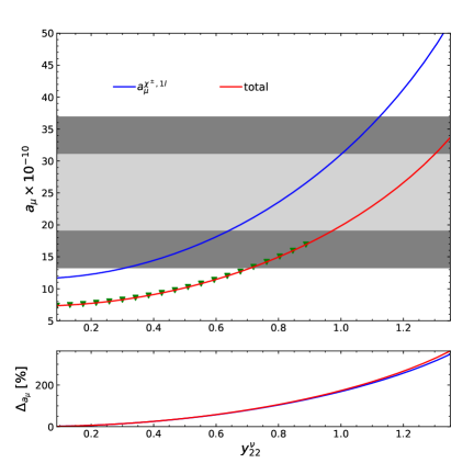
(a)

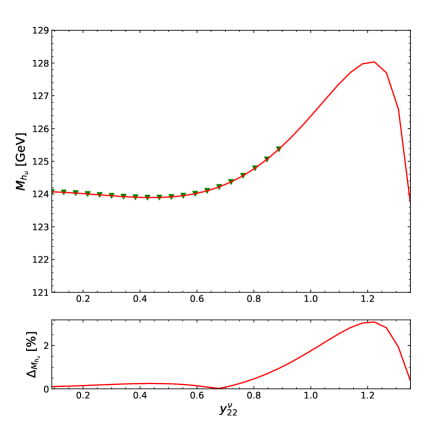
(b)

Figure 2: Upper left: The one-loop chargino contribution (blue) and the sum of all contributions (red) to the AMM of the muon in the NMSSM-nuSS. Lower left: The corresponding relative difference defined as $\Delta_{a_{\mu}}=\big{|}(a^{x}_{\mu}(\text{NMSSM-nuSS})-a^{x}_{\mu}(\text{NMSSM}))/a^{x}_{\mu}(\text{NMSSM})\big{|}$. Both as a function of $y_{22}^{\nu}$ in the $M_{X}$ parameterization. Upper right: The loop-corrected mass of the $h_{u}$-like Higgs boson in GeV at order $\mathcal{O}(\alpha_{t}\alpha_{s}+\alpha_{t}^{2})$. Lower right: The corresponding relative difference $\Delta_{M_{h_{u}}}=\left|(M_{h_{u}}^{\text{NMSSM-nuSS}}-M_{h_{u}}^{\text{NMSSM}})/M_{h_{u}}^{\text{\text{NMSSM}}}\right|$. Both as a function of $y_{22}^{\nu}$ in the $\mu_{X}$ parameterization.

In Fig. 2 we vary $y_{22}^{\nu}$ in the range $[0.9,1.35]$, keeping the other parameters fixed as in the parameter point P1 using the $\mu_{X}$ parameterization. If $y_{22}^{\nu}>1.45$, one enters the region where the sneutrino mass squared becomes negative. We remind the reader that $y_{22}^{\nu}$ enters the couplings between the muon, the charginos and the sneutrinos and also enters the mass matrix of the sneutrinos. Increasing $y_{22}^{\nu}$ leads to an increase of the mixing between the left-handed muon sneutrinos $\tilde{\nu}_{2}$, ${\tilde{N}}_{2}$, ${\tilde{X}}_{2}$, so that the mass of the $\tilde{\nu}_{2}$-like sneutrino becomes smaller while the mass of the ${\tilde{N}}_{2}$-like sneutrino increases. In the upper left plot, we show the dependence of the one-loop chargino contribution (blue) and the sum of all contributions (red) to the AMM of the muon in the NMSSM-nuSS as a function of $y_{22}^{\nu}$. We see a strong dependence on $y_{22}^{\nu}$ which can be understood by using an approximate expression for the new contribution from the one-loop chargino contribution in the NMSSM-nuSS. New contribution here means the difference between the one-loop chargino contribution in the NMSSM-nuSS and in the NMSSM. It can be obtained by using the mass insertion method. The Feynman diagram in Fig. 3 exemplifies the enhancement mechanism.

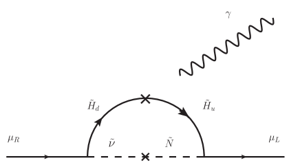
Figure 3: The new enhancement mechanism contributing to the anomalous magnetic moment of the muon in the NMSSM-nuSS.

In the region of large $y_{22}^{\nu}$, the approximate new contribution is given by

$$a_{\mu}^{\chi^{\pm},1l}(\text{new}) \sim -\frac{m_{l}}{8\pi^{2}}(y_{22}^{\nu})^{2}y_{\mu}\frac{\mu_{\text{eff}}^{2}v\text{Re}(s_{\beta}A^{\nu}_{22}e^{i\varphi_{u}}-c_{\beta}\mu_{\text{eff}})}{(M_{\tilde{\nu}_{+}\tilde{\nu}_{+}})_{22}-(M_{\tilde{N}_{+}\tilde{N}_{+}})_{22}}$$ (98)

$$(D_{1}((M_{\tilde{\nu}_{+}\tilde{\nu}_{+}})_{22},\mu_{\text{eff}}^{2},\mu_{\text{eff}}^{2},\mu_{\text{eff}}^{2})-D_{1}((M_{\tilde{N}_{+}\tilde{N}_{+}})_{22},\mu_{\text{eff}}^{2},\mu_{\text{eff}}^{2},\mu_{\text{eff}}^{2})),$$

where $D_{1}$ denotes the rank-1 four-point function where all external momenta are set equal to zero,

$$D_{1}(x,y,y,y)=-\frac{(2x^{2}+5xy-y^{2})}{12(x-y)^{3}y}+\frac{x^{2}\log(x/y)}{2(x-y)^{4}}\,,$$ (99)

and $(M_{\tilde{\nu}_{+}\tilde{\nu}_{+}})_{22},(M_{\tilde{N}_{+}\tilde{N}_{+}})_{22}$ are the second diagonal components of the sneutrino mass matrix, see Appendix A. This contribution is proportional to $(y_{22}^{\nu})^{2}$ in which one factor $y_{22}^{\nu}$ arises from the coupling $\tilde{H_{u}}\mu\tilde{N}$ and the other comes from the mixing between $\tilde{\nu}$ and $\tilde{N}$. In the upper left plot Fig. 2, we also highlighted the 1$\sigma$ (light gray) and the 2$\sigma$ (dark gray) regions of the difference between the experimental value and the SM prediction as defined in Eq. (4). The points denoted by green triangles are those points that pass all our constraints. In the lower left plot of Fig. 2 we show the relative difference between the muon AMM in the two models NMSSM and NMSSM-nuSS, defined as

$$\Delta_{a_{\mu}}=\bigg{|}\frac{(a^{x}_{\mu}(\text{NMSSM-nuSS})-a^{x}_{\mu}(\text{NMSSM}))}{a^{x}_{\mu}(\text{NMSSM})}\bigg{|}\,,$$ (100)

where $x$ can be the chargino one-loop contribution or the sum of all contributions. The relative difference is dominated by the chargino one-loop contribution and strongly increases with $y_{22}^{\nu}$ from 0 to more than 350% in the range of the $y_{22}^{\nu}$ variation. In the upper right plot of Fig. 2 we show the variation of the loop-corrected Higgs boson mass for the $h_{u}$-like state at order $\mathcal{O}(\alpha_{t}\alpha_{s}+\alpha_{t}^{2})$ as a function of $y_{22}^{\nu}$. As can be inferred from the plot, in the region $y_{22}^{\nu}>0.65$ the neutrino/sneutrino sector strongly affects the mass of the $h_{u}$-like Higgs boson. It increases until $y_{22}^{\nu}$ reaches $1.2$ and then quickly decreases. This is due to the interplay between the positive contributions from the neutrino one-loop diagrams and the negative contributions from the sneutrino one-loop diagrams. The variation of $y_{22}^{\nu}$ affects both contributions simultaneously. At large $y_{22}^{\nu}$ the sneutrino mass becomes very small so that its effect gets stronger than the neutrino one and it reduces the mass $M_{h_{u}}$ of the $h_{u}$-like Higgs boson to a very small value. The relative difference between the $h_{u}$-like Higgs boson mass in the NMSSM-nuSS and the NMSSM as function of $y_{22}^{\nu}$ is shown in the lower right plot of Fig. 2. From small values it increases starting from $y_{22}^{\nu}=0.65$ until it reaches a maximum of 3% at 1.2 and decreases again to small relative differences.

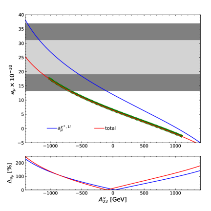
(a)

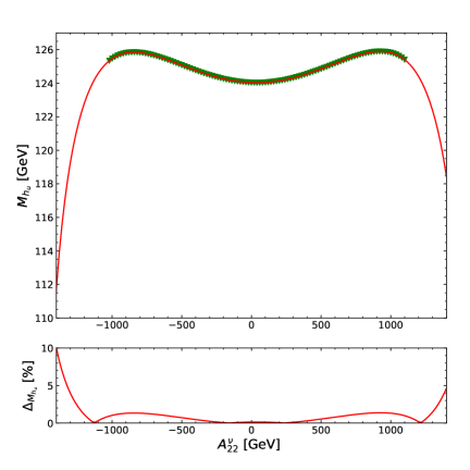
(b)

Figure 4: Similar to Fig. 2 but now $A^{\nu}_{22}$ is varied instead.

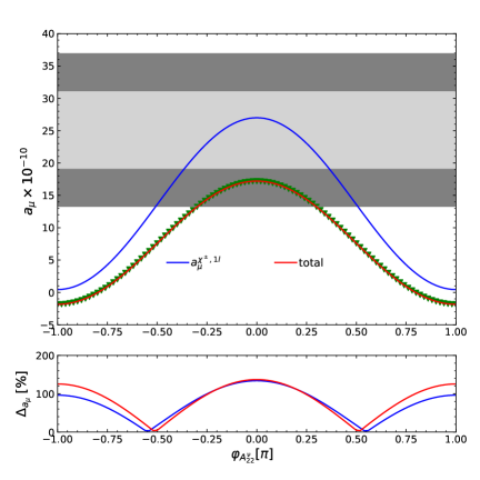
(a)

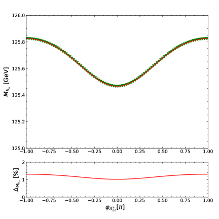
(b)

Figure 5: Effect of the complex phase of $A^{\nu}_{22}$ on the AMM of the muon (left) and the loop-corrected mass of the $h_{u}$-like Higgs boson. The color code is the same as Fig. 2.

Dependence on $A_{22}^{\nu}$:

The dependence of the muon AMM and the loop-corrected $h_{u}$-like Higgs boson mass on the magnitude of the neutrino soft SUSY-breaking trilinear coupling $A_{22}^{\nu}$ is presented in Fig. 4. We varied $A_{22}^{\nu}$ in the range $[-1400,1400]\,\leavevmode\nobreak\ \text{GeV}$. The notation and color code is the same as in Fig. 2. The nearly linear dependence of the chargino one-loop contribution seen in Fig. 4 (upper left) can be explained by using the approximate expression in Eq. (98). The change of the sign of the new contribution around $A_{22}^{\nu}\sim 0$ can be seen in the lower left plot of Fig. 4. For the explanation of the experimental result for $(g-2)_{\mu}$ a negative value of $A_{22}^{\nu}$ is preferred. This feature gives also a possibility for the NMSSM-nuSS to explain simutaneously both the positive discrepancy in $(g-2)_{\mu}$ and the negative discrepancy in $(g-2)_{e}$ [62, 63, 64] by choosing a negative value for $A_{22}^{\nu}$ and a positive value for $A_{11}^{\nu}$ as shown in [35]. For the parameter point P1, it is impossible to obtain the SUSY contributions for the electron AMM of $-7\times 10^{-13}$ to be close to the deviation between the experimental measurement and the SM prediction while it still satisfies other constraints. In the right plots of Fig. 4, we can see the dependence of the loop-corrected $h_{u}$-like Higgs boson mass on $A_{22}^{\nu}$ in the upper plot while in the lower plot we see the relative difference of this mass in the two models with and without inverse seesaw mechanism. The larger the magnitude of $A_{22}^{\nu}$ is, the larger the mixing between $\tilde{\nu}$ and $\tilde{N}$ becomes. This leads to the reduction of the mass of the left-handed muon-like sneutrino. As a consequence the sneutrino contributions become dominant compared to the neutrino contributions.

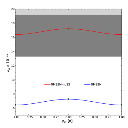
(a)

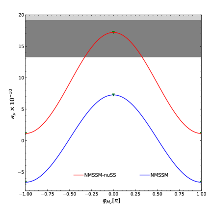
(b)

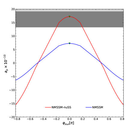
(c)

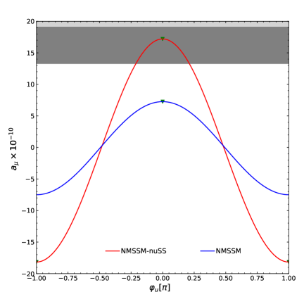
(d)

Figure 6: The AMM of the muon in the NMSSM with (red) and without (blue) inverse seesaw mechanism as a function of several CP-violating phases: (a) $\varphi_{M_{1}}$, (b) $\varphi_{M_{2}}$, (c) $\varphi_{\mu_{\text{eff}}}$, (d) $\varphi_{u}$.

Influence of the CP-violating phases:

We now discuss the influence of the CP-violating phases on the muon AMM and the loop-corrected $h_{u}$-like Higgs boson mass. In Fig. 5, we vary the complex phase of $A^{\nu}_{22}$ in the range $[-\pi,\pi]$. The SUSY contributions to $a_{\mu}$ change its value from $-2\times 10^{-10}$ at $\varphi_{A^{\nu}_{22}}=-\pi$ to reach a maximum of $17.2\times 10^{-10}$ at $\varphi_{A^{\nu}_{22}}=0$ and then reduce it back to $-2\times 10^{-10}$ at $\varphi_{A^{\nu}_{22}}=\pi$. While the complex phase of $A^{\nu}_{22}$ strongly affects the $(g-2)_{\mu}$, its effect on the mass of the $h_{u}$-like Higgs boson is rather mild as can seen in the right plots of Fig. 5. We further present in Fig. 6 the influence of several complex phases, namely $\varphi_{M_{1}},\varphi_{M_{2}},\varphi_{\mu_{\text{eff}}},\varphi_{u}$, on the SUSY contributions to $a_{\mu}$ in both models, the NMSSM with and without inverse seesaw mechanism. In all these plots, the NMSSM-nuSS results are plotted in red while the blue lines show the results in the NMSSM without inverse seesaw mechanism. The complex phase of $M_{1}$ enters only the neutralino contribution. Figure 6 (a) shows a mild dependence of $(g-2)_{\mu}$ on this phase for this particular point where the neutralino contribution is always negative and about four times smaller than the dominant chargino contribution. The complex phase of $M_{2}$ enters not only the neutralino contribution but also the chargino one. In Fig. 6 (b) we can see a similar dependence of $(g-2)_{\mu}$ on this phase in both models. The two remaining phases $\varphi_{\mu_{\text{eff}}}$ and $\varphi_{u}$ have a stronger influence on $(g-2)_{\mu}$ in the NMSSM-nuSS than in the NMSSM without ISS as shown in Fig. 6 (c) and Fig. 6 (d). This is due to these two phases entering the new contribution in the NMSSM-nuSS, see Eq. (98). Note that in Fig. 6 (c) the range of $\varphi_{\mu_{\text{eff}}}$ is $[-0.8\pi,08\pi]$ since outside this range the mass of the $h_{u}$-like Higgs boson turns out to be negative. For illustrative purpose we show partly the light gray and dark gray regions representing the 1$\sigma$ and 2$\sigma$ deviations between the experimental measurement and the SM prediction for $(g-2)_{\mu}$. In these plots, except for the points where the phases $\varphi_{M_{1}},\phi_{M_{2}},\varphi_{\mu_{\text{eff}}},\varphi_{u}$ are close to zero or $\pm\pi$, all other points are ruled out because of the constraints on the electric dipole moments of the electron.

Effects on the electron EDM:

We now investigate the effect of the new complex phase in the (s)neutrino sectors on the electron EDM. In NMSSMCALC, the electron, neutron, Thallium and Mercury EDMs have been implemented as described in [47]. We follow the conventions in NMSSMCALC that all EDMs are normalized to their corresponding experimental upper bounds. A thorough investigation of the complex phases in the NMSSM on the electron, neutron, Thallium and Mercury EDMs in [47] has shown that the complex phases of the electroweak sector such as $\varphi_{M_{1}},\varphi_{M_{2}},$ $\varphi_{1}\equiv\varphi_{\lambda}+\varphi_{s}+\varphi_{u},\varphi_{2}\equiv\varphi_{\kappa}+3\varphi_{s}$ have the strongest effects on the electron EDM which also enters the Thallium and Mercury EDMs. These phases contribute to the electron EDM through the one-loop neutralino and chargino contributions as can be inferred from the second terms in Eq. (43) and Eq. (42). Apart from the NMSSM-like phase $\varphi_{2}$, the stringent limit on the electron EDM has ruled out almost any non-vanishing value of these complex phases as we also observe in this study (see previous paragraph). In the NMSSM-nuSS, there are new complex phases from the neutrino sector, $\delta_{CP},\varphi_{y^{\nu}_{11}},\varphi_{\mu^{X}_{11}}$, $\varphi_{\lambda^{X}_{11}}$, and from the sneutrino sector $\varphi_{A^{\nu}_{11}},\varphi_{A^{X}_{11}},\varphi_{B^{\mu_{X}}_{11}}$. However, only the complex phase $\varphi_{A^{\nu}_{11}}$ gives a significant contribution to the EDMs, all other remaining phases have a negligible effect. The complex phase $\varphi_{A^{\nu}_{11}}$ appears in the one-loop chargino contribution, see the second term in Eq. (42). This provides a possibility for the reduction of the imarginary part of the coupling $g^{R}_{l\tilde{\chi}^{-}_{j}\tilde{\nu}_{i}}$, see Eq. (46), and may thereby lead to the cancellation between different contributions to the electron EDM. Such a cancellation can never happen in the NMSSM without ISS.

To illustrate this, we show in Fig. 7 the dependence of the electron EDM, normalized to the experimental upper bound, on the complex phase of $A^{\nu}_{11}$ using the parameter point P1. In the left plot, we have set $\varphi_{M_{1}}=\pi/2$ while in the right plot we have set $\varphi_{M_{2}}=\pi/138$. All other phases are equal to zero. These values of $\varphi_{M_{1}}$ and $\varphi_{M_{2}}$ correspond to the largest possible induced EDM of the neutron from the respective phases that still remains below the experimental upper bound. The red (blue) lines show the electron EDMs in the NMSSM with (without) ISS. As can be inferred from the plots, in the NMSSM without ISS the electron EDM is about $25$ times larger than its experimental upper bound for $\varphi_{M_{1}}=\pi/2$ and about 102 times larger for $\varphi_{M_{2}}=\pi/138$. In the NMSSM with ISS a cancellation of all contributions to the electron EDM takes place at $\varphi_{A_{11}^{\nu}}=-0.0055\pi$ for $\varphi_{M_{1}}=\pi/2$ and at $\varphi_{A_{11}^{\nu}}=0.022\pi$ for $\varphi_{M_{2}}=\pi/138$ so that the electron EDM is pushed below its experimental upper bound. Note that all the points with the electron EDM being less than one satisfy all our constraints mentioned in this paper. A similar cancellation can also happen for the phases $\varphi_{1}$ and $\varphi_{2}$.

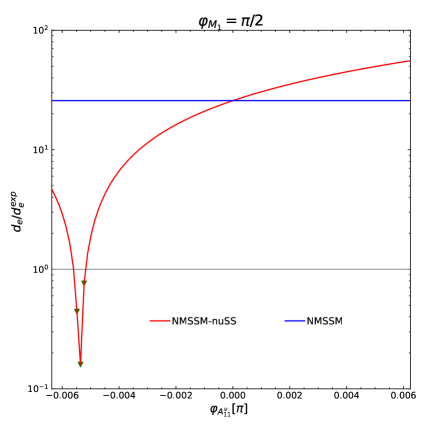
(a)

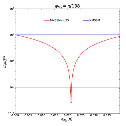
(b)

Figure 7: The EDM of the electron in the NMSSM with (red) and without (blue) inverse seesaw mechanism as a function of the complex phase of $A^{\nu}_{11}$ where (a) $\varphi_{M_{1}}=\pi/2$, (b) $\varphi_{M_{2}}=\pi/138$.

5 Conclusions

In this paper we have computed the full one-loop SUSY contributions and the two-loop Barr-Zee-type diagrams with $h\gamma\gamma$ effective couplings to the AMM and EDM of charged leptons in two models, the NMSSM with and without inverse seesaw mechanism including CP-violating phases. We presented the analytic expressions and implemented them in the two Fortran codes NMSSMCALC and NMSSMCALC-nuSS, which compute the Higgs boson masses and mixings, together with the Higgs boson decay branching ratios taking into account the most up-to-date higher-order corrections. Using a typical parameter point with an intermediate value of $\tan\beta$ and large charged Higgs mass, we have investigated in the NMSSM with inverse seesaw mechanism the effect of the (s)neutrino sector on the muon AMM in comparison with its effect on the SM-like Higgs-boson mass. We see a large positive contribution to the AMM from the mixing between the left-handed muon-type sneutrino and the right-handed one (denoted as $\tilde{N}$ in the previous sections) provided that the muon-type neutrino Yukawa coupling is of order ${\cal O}(1)$, that the muon-type neutrino trilinear coupling is negative and that the left- and right-handed muon-type sneutrino masses are small. Too light sneutrino masses, however, give a large negative correction to the Higgs boson masses. In order to compensate this negative effect one should also require light sterile neutrino masses. Therefore, there is a strong correlation between the effects of the (s)neutrino sector on the two observables. We have also found a strong effect of the CP-violating phases on the AMM of the muon in the two models.

For the electron EDM we found that the complex phase of the sneutrino sector $\varphi_{A^{\nu}_{11}}$ gives a significant contribution at one-loop level. This provides a possibility for the cancellation of the different contributions to the electron EDM so that it remains below the experimental upper bound. While most of the non-vanishing complex phases of the electroweak sector of the NMSSM have been ruled out by the constraint on the electron EDM, in the NMSSM-nuSS one can remain in the region of validity with an appropriately chosen value of $\varphi_{A^{\nu}_{11}}$.

Finally, the calculations presented in this paper have been implemented in the programs NMSSMCALC and NMSSMCALC-nuSS which are publicly available.

Appendix A The Sneutrino Mass Matrix

Here we provide the mass matrix of the sneutrinos. Each entry is a $3\times 3$ matrix in the flavor space.

$$(M_{\tilde{\nu}})_{{\tilde{\nu}}_{+}{\tilde{\nu}}_{+}} =\frac{1}{2}I_{3}M_{z}^{2}\cos 2\beta+\frac{1}{2}\left(\tilde{m}_{L}^{2}+\tilde{m}_{L}^{2T}\right)+\frac{1}{2}v_{u}^{2}\text{Re}\left(y_{\nu}y_{\nu}^{\dagger}\right)$$ (101)

$$(M_{\tilde{\nu}})_{{\tilde{\nu}}_{+}{\tilde{N}}_{+}} =\frac{1}{\sqrt{2}}v_{u}\text{Re}\left(e^{i\varphi_{u}}y_{\nu}A_{\nu}\right)-\frac{1}{2}v_{d}v_{s}\text{Re}\left(e^{i\varphi_{s}}\lambda y_{\nu}^{*}\right)$$ (102)

$$(M_{\tilde{\nu}})_{{\tilde{\nu}}_{+}{\tilde{X}}_{+}} =\frac{1}{\sqrt{2}}v_{u}\text{Re}\left(e^{i\varphi_{u}}y_{\nu}\mu_{X}^{*}\right)$$ (103)

$$(M_{\tilde{\nu}})_{{\tilde{\nu}}_{+}{\tilde{\nu}}_{-}} =\frac{i}{2}\left(\tilde{m}_{L}^{2}-\tilde{m}_{L}^{2T}\right)+\frac{1}{2}v_{u}^{2}\text{Im}\left(y_{\nu}y_{\nu}^{\dagger}\right)$$ (104)

$$(M_{\tilde{\nu}})_{{\tilde{\nu}}_{+}{\tilde{N}}_{-}} =\frac{1}{\sqrt{2}}v_{u}\text{Im}\left(e^{i\varphi_{u}}y_{\nu}A_{\nu}\right)-\frac{1}{2}v_{d}v_{s}\text{Im}\left(e^{i\varphi_{s}}\lambda y_{\nu}^{*}\right)$$ (105)

$$(M_{\tilde{\nu}})_{{\tilde{\nu}}_{+}{\tilde{X}}_{-}} =\frac{1}{\sqrt{2}}v_{u}\text{Im}\left(e^{i\varphi_{u}}y_{\nu}\mu_{X}^{*}\right)$$ (106)

$$(M_{\tilde{\nu}})_{{\tilde{N}}_{+}{\tilde{N}}_{+}} =\frac{1}{2}\left(\tilde{m}^{2}_{N}+\tilde{m}^{2T}_{N}\right)+\text{Re}\left(\mu_{X}\mu_{X}^{\dagger}\right)+\frac{1}{2}v_{u}^{2}\text{Re}\left(y_{\nu}^{T}y_{\nu}^{*}\right)$$ (107)

$$(M_{\tilde{\nu}})_{{\tilde{N}}_{+}{\tilde{X}}_{+}} =\text{Re}\left(\mu_{X}B_{\mu_{X}}\right)+\frac{1}{\sqrt{2}}v_{s}\text{Re}\left[e^{-i\varphi_{s}}\mu_{X}\left(\lambda_{X}^{\dagger}+\lambda_{X}^{*}\right)\right]$$ (108)

$$(M_{\tilde{\nu}})_{{\tilde{N}}_{+}{\tilde{\nu}}_{-}} =-\frac{1}{\sqrt{2}}v_{u}\text{Im}\left(e^{i\varphi_{u}}A_{\nu}^{T}y_{\nu}^{T}\right)-\frac{1}{2}v_{d}v_{s}\text{Im}\left(e^{i\varphi_{s}}\lambda y_{\nu}^{\dagger}\right)$$ (109)

$$(M_{\tilde{\nu}})_{{\tilde{N}}_{+}{\tilde{N}}_{-}} =\frac{i}{2}\left(\tilde{m}^{2}_{N}-\tilde{m}^{2T}_{N}\right)-\text{Im}\left(\mu_{X}\mu_{X}^{\dagger}\right)-\frac{1}{2}v_{u}^{2}\text{Im}\left(y_{\nu}^{T}y_{\nu}^{*}\right)$$ (110)

$$(M_{\tilde{\nu}})_{{\tilde{N}}_{+}{\tilde{X}}_{-}} =-\text{Im}\left(\mu_{X}B_{\mu_{X}}\right)+\frac{1}{\sqrt{2}}v_{s}\text{Im}\left[e^{-i\varphi_{s}}\mu_{X}\left(\lambda_{X}^{\dagger}+\lambda_{X}^{*}\right)\right]$$ (111)

$$(M_{\tilde{\nu}})_{{\tilde{X}}_{+}{\tilde{X}}_{+}} =\frac{1}{2}\left(\tilde{m}_{X}^{2}+\tilde{m}_{X}^{2T}\right)+\text{Re}\left(\mu_{X}^{T}\mu_{X}^{*}\right)+\frac{1}{2}\text{Re}\left[\left(e^{2i\varphi_{s}}v_{s}^{2}\kappa-e^{i\varphi_{u}}v_{d}v_{u}\lambda\right)\left(\lambda_{X}^{*}+\lambda_{X}^{\dagger}\right)\right]$$

$$\quad+\frac{1}{2}v_{s}^{2}\text{Re}\left[\left(\lambda_{X}+\lambda_{X}^{T}\right)\left(\lambda_{X}^{\dagger}+\lambda_{X}^{*}\right)\right]+\frac{1}{\sqrt{2}}v_{s}\text{Re}\left[e^{i\varphi_{s}}\left(\lambda_{X}A_{X}+A_{X}^{T}\lambda_{X}^{T}\right)\right]$$ (112)

$$(M_{\tilde{\nu}})_{{\tilde{X}}_{+}{\tilde{\nu}}_{-}} =-\frac{1}{\sqrt{2}}v_{u}\text{Im}\left(e^{i\varphi_{u}}\mu_{X}^{\dagger}y_{\nu}^{T}\right)$$ (113)

$$(M_{\tilde{\nu}})_{{\tilde{X}}_{+}{\tilde{N}}_{-}} =\text{Im}\left(B_{\mu_{X}}^{T}\mu_{X}^{T}\right)+\frac{1}{\sqrt{2}}v_{s}\text{Im}\left[e^{-i\varphi_{s}}\left(\lambda_{X}^{\dagger}+\lambda_{X}^{*}\right)\mu^{T}_{X}\right]$$ (114)

$$(M_{\tilde{\nu}})_{{\tilde{X}}_{+}{\tilde{X}}_{-}} =\frac{i}{2}\left(\tilde{m}_{X}^{2}-\tilde{m}_{X}^{2T}\right)+\text{Im}\left(\mu_{X}^{T}\mu_{X}^{*}\right)+\frac{1}{2}\text{Im}\left[\left(e^{2i\varphi_{s}}v_{s}^{2}\kappa-e^{i\varphi_{u}}v_{d}v_{u}\lambda\right)\left(\lambda_{X}^{*}+\lambda_{X}^{\dagger}\right)\right]$$

$$\quad+\frac{1}{2}v_{s}^{2}\text{Im}\left[\left(\lambda_{X}+\lambda_{X}^{T}\right)\left(\lambda_{X}^{\dagger}+\lambda_{X}^{*}\right)\right]-\frac{1}{\sqrt{2}}v_{s}\text{Im}\left[e^{i\varphi_{s}}\left(\lambda_{X}A_{X}+A_{X}^{T}\lambda_{X}^{T}\right)\right]$$ (115)

$$(M_{\tilde{\nu}})_{{\tilde{\nu}}_{-}{\tilde{\nu}}_{-}} =\frac{1}{2}I_{3}M_{z}^{2}\cos 2\beta+\frac{1}{2}\left(\tilde{m}_{L}^{2}+\tilde{m}_{L}^{2T}\right)+\frac{1}{2}v_{u}^{2}\text{Re}\left(y_{\nu}y_{\nu}^{\dagger}\right)$$ (116)

$$(M_{\tilde{\nu}})_{{\tilde{\nu}}_{-}{\tilde{N}}_{-}} =\frac{1}{\sqrt{2}}v_{u}\text{Re}\left(e^{i\varphi_{u}}y_{\nu}A_{\nu}\right)-\frac{1}{2}v_{d}v_{s}\text{Re}\left(e^{i\varphi_{s}}\lambda y_{\nu}^{*}\right)$$ (117)

$$(M_{\tilde{\nu}})_{{\tilde{\nu}}_{-}{\tilde{X}}_{-}} =\frac{1}{\sqrt{2}}v_{u}\text{Re}\left(e^{i\varphi_{u}}y_{\nu}\mu_{X}^{*}\right)$$ (118)

$$(M_{\tilde{\nu}})_{{\tilde{N}}_{-}{\tilde{N}}_{-}} =\frac{1}{2}\left(\tilde{m}^{2}_{N}+\tilde{m}^{2T}_{N}\right)+\text{Re}\left(\mu_{X}\mu_{X}^{\dagger}\right)+\frac{1}{2}v_{u}^{2}\text{Re}\left(y_{\nu}^{T}y_{\nu}^{*}\right)$$ (119)

$$(M_{\tilde{\nu}})_{{\tilde{N}}_{-}{\tilde{X}}_{-}} =\text{Re}\left(\mu_{X}B_{\mu_{X}}\right)-\frac{1}{\sqrt{2}}v_{s}\text{Re}\left[e^{-i\varphi_{s}}\mu_{X}\left(\lambda_{X}^{\dagger}+\lambda_{X}^{*}\right)\right]$$ (120)

$$(M_{\tilde{\nu}})_{{\tilde{X}}_{-}{\tilde{X}}_{-}} =\frac{1}{2}\left(\tilde{m}_{X}^{2}+\tilde{m}_{X}^{2T}\right)+\text{Re}\left(\mu_{X}^{T}\mu_{X}^{*}\right)-\frac{1}{2}\text{Re}\left[\left(e^{2i\varphi_{s}}v_{s}^{2}\kappa-e^{i\varphi_{u}}v_{d}v_{u}\lambda\right)\left(\lambda_{X}^{*}+\lambda_{X}^{\dagger}\right)\right]$$

$$\quad+\frac{1}{2}v_{s}^{2}\text{Re}\left[\left(\lambda_{X}+\lambda_{X}^{T}\right)\left(\lambda_{X}^{\dagger}+\lambda_{X}^{*}\right)\right]-\frac{1}{\sqrt{2}}v_{s}\text{Re}\left[e^{i\varphi_{s}}\left(\lambda_{X}A_{X}+A_{X}^{T}\lambda_{X}^{T}\right)\right].$$ (121)

References

- [1] Muon g-2 collaboration, B. Abi et al., Measurement of the Positive Muon Anomalous Magnetic Moment to 0.46 ppm, Phys. Rev. Lett. 126 (2021) 141801, [2104.03281].
- [2] Muon g-2 collaboration, G. W. Bennett et al., Final Report of the Muon E821 Anomalous Magnetic Moment Measurement at BNL, Phys. Rev. D 73 (2006) 072003, [hep-ex/0602035].
- [3] T. Aoyama et al., The anomalous magnetic moment of the muon in the Standard Model, Phys. Rept. 887 (2020) 1–166, [2006.04822].
- [4] T. Aoyama, M. Hayakawa, T. Kinoshita and M. Nio, Complete Tenth-Order QED Contribution to the Muon g-2, Phys. Rev. Lett. 109 (2012) 111808, [1205.5370].
- [5] E.-H. Chao, R. J. Hudspith, A. Gérardin, J. R. Green, H. B. Meyer and K. Ottnad, Hadronic light-by-light contribution to from lattice QCD: a complete calculation, Eur. Phys. J. C 81 (2021) 651, [2104.02632].
- [6] A. Czarnecki and W. J. Marciano, The Muon anomalous magnetic moment: A Harbinger for ’new physics’, Phys. Rev. D 64 (2001) 013014, [hep-ph/0102122].
- [7] P. Fayet, Supergauge Invariant Extension of the Higgs Mechanism and a Model for the electron and Its Neutrino, Nucl. Phys. B 90 (1975) 104–124.
- [8] R. Barbieri, S. Ferrara and C. A. Savoy, Gauge Models with Spontaneously Broken Local Supersymmetry, Phys.Lett. B119 (1982) 343.
- [9] M. Dine, W. Fischler and M. Srednicki, A Simple Solution to the Strong CP Problem with a Harmless Axion, Phys.Lett. B104 (1981) 199.
- [10] H. P. Nilles, M. Srednicki and D. Wyler, Weak Interaction Breakdown Induced by Supergravity, Phys.Lett. B120 (1983) 346.
- [11] J. Frere, D. Jones and S. Raby, Fermion Masses and Induction of the Weak Scale by Supergravity, Nucl.Phys. B222 (1983) 11.
- [12] J. Derendinger and C. A. Savoy, Quantum Effects and SU(2) x U(1) Breaking in Supergravity Gauge Theories, Nucl.Phys. B237 (1984) 307.
- [13] J. R. Ellis, J. Gunion, H. E. Haber, L. Roszkowski and F. Zwirner, Higgs Bosons in a Nonminimal Supersymmetric Model, Phys. Rev. D 39 (1989) 844.
- [14] M. Drees, Supersymmetric Models with Extended Higgs Sector, Int. J. Mod. Phys. A 4 (1989) 3635.
- [15] U. Ellwanger, M. Rausch de Traubenberg and C. A. Savoy, Particle spectrum in supersymmetric models with a gauge singlet, Phys. Lett. B 315 (1993) 331–337, [hep-ph/9307322].
- [16] U. Ellwanger, M. Rausch de Traubenberg and C. A. Savoy, Higgs phenomenology of the supersymmetric model with a gauge singlet, Z. Phys. C 67 (1995) 665–670, [hep-ph/9502206].
- [17] U. Ellwanger, M. Rausch de Traubenberg and C. A. Savoy, Phenomenology of supersymmetric models with a singlet, Nucl.Phys. B492 (1997) 21–50, [hep-ph/9611251].
- [18] T. Elliott, S. King and P. White, Unification constraints in the next-to-minimal supersymmetric standard model, Phys.Lett. B351 (1995) 213–219, [hep-ph/9406303].
- [19] S. King and P. White, Resolving the constrained minimal and next-to-minimal supersymmetric standard models, Phys.Rev. D52 (1995) 4183–4216, [hep-ph/9505326].
- [20] F. Franke and H. Fraas, Neutralinos and Higgs bosons in the next-to-minimal supersymmetric standard model, Int.J.Mod.Phys. A12 (1997) 479–534, [hep-ph/9512366].
- [21] M. Maniatis, The Next-to-Minimal Supersymmetric extension of the Standard Model reviewed, Int. J. Mod. Phys. A 25 (2010) 3505–3602, [0906.0777].
- [22] U. Ellwanger, C. Hugonie and A. M. Teixeira, The Next-to-Minimal Supersymmetric Standard Model, Phys. Rept. 496 (2010) 1–77, [0910.1785].
- [23] M. Krawczyk, Precision muon g-2 results and light Higgs bosons in the 2HDM(II), Acta Phys. Polon. B 33 (2002) 2621–2634, [hep-ph/0208076].
- [24] F. Domingo and U. Ellwanger, Constraints from the Muon g-2 on the Parameter Space of the NMSSM, JHEP 07 (2008) 079, [0806.0733].
- [25] R. Mohapatra, Mechanism for Understanding Small Neutrino Mass in Superstring Theories, Phys. Rev. Lett. 56 (1986) 561–563.
- [26] R. N. Mohapatra and J. W. F. Valle, Neutrino mass and baryon-number nonconservation in superstring models, Phys. Rev. D 34 (Sep, 1986) 1642–1645.
- [27] J. Bernabeu, A. Santamaria, J. Vidal, A. Mendez and J. Valle, Lepton Flavor Nonconservation at High-Energies in a Superstring Inspired Standard Model, Phys. Lett. B 187 (1987) 303–308.
- [28] I. Gogoladze, N. Okada and Q. Shafi, NMSSM and Seesaw Physics at LHC, Phys. Lett. B672 (2009) 235–239, [0809.0703].
- [29] I. Gogoladze, B. He and Q. Shafi, Inverse Seesaw in NMSSM and 126 GeV Higgs Boson, Phys. Lett. B718 (2013) 1008–1013, [1209.5984].
- [30] W. Wang, J. M. Yang and L. L. You, Higgs boson mass in NMSSM with right-handed neutrino, JHEP 07 (2013) 158, [1303.6465].
- [31] T. N. Dao, M. Mühlleitner and A. V. Phan, Loop-corrected Higgs Masses in the NMSSM with Inverse Seesaw Mechanism, 2108.10088.
- [32] J. Cao, Y. He, Y. Pan, Y. Yue, H. Zhou and P. Zhu, Impact of leptonic unitarity and dark matter direct detection experiments on the NMSSM with inverse seesaw mechanism, JHEP 12 (2020) 023, [1903.01124].
- [33] J. Cao, L. Meng, Y. Yue, H. Zhou and P. Zhu, Suppressing the scattering of WIMP dark matter and nucleons in supersymmetric theories, Physical Review D 101 (apr, 2020) .
- [34] J. Cao, J. Lian, L. Meng, Y. Yue and P. Zhu, Anomalous muon magnetic moment in the inverse seesaw extended next-to-minimal supersymmetric standard model, Phys. Rev. D 101 (2020) 095009, [1912.10225].
- [35] J. Cao, Y. He, J. Lian, D. Zhang and P. Zhu, Electron and muon anomalous magnetic moments in the inverse seesaw extended NMSSM, Phys. Rev. D 104 (2021) 055009, [2102.11355].
- [36] J. Baglio, R. Gröber, M. Mühlleitner, D. Nhung, H. Rzehak, M. Spira et al., NMSSMCALC: A Program Package for the Calculation of Loop-Corrected Higgs Boson Masses and Decay Widths in the (Complex) NMSSM, Comput. Phys. Commun. 185 (2014) 3372–3391.
- [37] T. Graf, R. Grober, M. Muhlleitner, H. Rzehak and K. Walz, Higgs Boson Masses in the Complex NMSSM at One-Loop Level, JHEP 10 (2012) 122.
- [38] M. Mühlleitner, D. T. Nhung, H. Rzehak and K. Walz, Two-loop contributions of the order to the masses of the Higgs bosons in the CP-violating NMSSM, JHEP 05 (2015) 128, [1412.0918].
- [39] T. Dao, R. Gröber, M. Krause, M. Mühlleitner and H. Rzehak, Two-loop ( ) corrections to the neutral Higgs boson masses in the CP-violating NMSSM, JHEP 08 (2019) 114.
- [40] T. N. Dao, M. Gabelmann, M. Mühlleitner and H. Rzehak, Two-loop ((t + λ + κ)2) corrections to the Higgs boson masses in the CP-violating NMSSM, JHEP 09 (2021) 193, [2106.06990].
- [41] J. A. Casas and A. Ibarra, Oscillating neutrinos and , Nucl. Phys. B618 (2001) 171–204, [hep-ph/0103065].
- [42] E. Arganda, M. J. Herrero, X. Marcano and C. Weiland, Imprints of massive inverse seesaw model neutrinos in lepton flavor violating Higgs boson decays, Phys. Rev. D 91 (2015) 015001, [1405.4300].
- [43] F. Jegerlehner and A. Nyffeler, The Muon g-2, Phys. Rept. 477 (2009) 1–110, [0902.3360].
- [44] L. Lavoura, General formulae for f(1) — f(2) gamma, Eur. Phys. J. C 29 (2003) 191–195, [hep-ph/0302221].
- [45] H. H. Patel, Package-X: A Mathematica package for the analytic calculation of one-loop integrals, Comput. Phys. Commun. 197 (2015) 276–290, [1503.01469].
- [46] T. Moroi, The Muon anomalous magnetic dipole moment in the minimal supersymmetric standard model, Phys. Rev. D 53 (1996) 6565–6575, [hep-ph/9512396].
- [47] S. F. King, M. Muhlleitner, R. Nevzorov and K. Walz, Exploring the CP-violating NMSSM: EDM Constraints and Phenomenology, Nucl. Phys. B 901 (2015) 526–555, [1508.03255].
- [48] C.-H. Chen and C. Q. Geng, The Muon anomalous magnetic moment from a generic charged Higgs with SUSY, Phys. Lett. B 511 (2001) 77–84, [hep-ph/0104151].
- [49] A. Arhrib and S. Baek, Two loop Barr-Zee type contributions to (g-2)(muon) in the MSSM, Phys. Rev. D 65 (2002) 075002, [hep-ph/0104225].
- [50] S. Heinemeyer, D. Stockinger and G. Weiglein, Two loop SUSY corrections to the anomalous magnetic moment of the muon, Nucl. Phys. B 690 (2004) 62–80, [hep-ph/0312264].
- [51] S. Heinemeyer, D. Stockinger and G. Weiglein, Electroweak and supersymmetric two-loop corrections to (g-2)(mu), Nucl. Phys. B 699 (2004) 103–123, [hep-ph/0405255].
- [52] P. von Weitershausen, M. Schafer, H. Stockinger-Kim and D. Stockinger, Photonic SUSY Two-Loop Corrections to the Muon Magnetic Moment, Phys. Rev. D 81 (2010) 093004, [1003.5820].
- [53] H. G. Fargnoli, C. Gnendiger, S. Paßehr, D. Stöckinger and H. Stöckinger-Kim, Non-decoupling two-loop corrections to from fermion/sfermion loops in the MSSM, Phys. Lett. B 726 (2013) 717–724, [1309.0980].
- [54] H. Fargnoli, C. Gnendiger, S. Paßehr, D. Stöckinger and H. Stöckinger-Kim, Two-loop corrections to the muon magnetic moment from fermion/sfermion loops in the MSSM: detailed results, JHEP 02 (2014) 070, [1311.1775].
- [55] K. Cheung, O. C. W. Kong and J. S. Lee, Electric and anomalous magnetic dipole moments of the muon in the MSSM, JHEP 06 (2009) 020, [0904.4352].
- [56] G. Degrassi and G. F. Giudice, QED logarithms in the electroweak corrections to the muon anomalous magnetic moment, Phys. Rev. D 58 (1998) 053007, [hep-ph/9803384].
- [57] S. M. Barr and A. Zee, Electric Dipole Moment of the Electron and of the Neutron, Phys. Rev. Lett. 65 (1990) 21–24.
- [58] T. Abe, J. Hisano, T. Kitahara and K. Tobioka, Gauge invariant Barr-Zee type contributions to fermionic EDMs in the two-Higgs doublet models, JHEP 01 (2014) 106, [1311.4704].
- [59] P. Bechtle, D. Dercks, S. Heinemeyer, T. Klingl, T. Stefaniak, G. Weiglein et al., HiggsBounds-5: Testing Higgs Sectors in the LHC 13 TeV Era, Eur. Phys. J. C 80 (2020) 1211, [2006.06007].
- [60] P. Bechtle, S. Heinemeyer, T. Klingl, T. Stefaniak, G. Weiglein and J. Wittbrodt, HiggsSignals-2: Probing new physics with precision Higgs measurements in the LHC 13 TeV era, Eur. Phys. J. C 81 (2021) 145, [2012.09197].
- [61] Particle Data Group collaboration, P. Zyla et al., Review of Particle Physics, PTEP 2020 (2020) 083C01.
- [62] T. Aoyama, T. Kinoshita and M. Nio, Revised and Improved Value of the QED Tenth-Order Electron Anomalous Magnetic Moment, Phys. Rev. D 97 (2018) 036001, [1712.06060].
- [63] D. Hanneke, S. Fogwell and G. Gabrielse, New measurement of the electron magnetic moment and the fine structure constant, Physical Review Letters 100 (mar, 2008) .
- [64] D. Hanneke, S. Fogwell Hoogerheide and G. Gabrielse, Cavity control of a single-electron quantum cyclotron: Measuring the electron magnetic moment, Phys. Rev. A 83 (May, 2011) 052122.