Ab initio material design of Ag-based oxides for high-$T_{c}$ superconductor

Abstract

We propose silver-based oxides with layered perovskite structure as candidates of exhibiting intriguing feature of strongly correlated electrons. The compounds show unique covalence between Ag $d$ and O $p$ orbitals with the strong electron correlation of their antibonding orbital similar to the copper oxide high-temperature superconductors, but stronger covalency and slightly smaller correlation strength. We examine $A_{2}$AgO₂X₂ with $A=$Sr and Ba and $X=$F, I and Cl in detail. Among them, Sr₂AgO₂F₂ has the largest effective onsite Coulomb repulsion and shows an antiferromagnetic insulating ground state, which competes with correlated metals. It offers features both similar and distinct from the copper oxides, and paves a new route. The possibility of superconductivity in doped systems is discussed.

I Introduction

Copper oxides with layered perovskite structure (abbreviated as cuprates hereafter) bednortz exhibit spectacular properties with high-temperature superconducting phases above 100K, which is the highest record so far at ambient pressure. Above the superconducting critical temperature, they show enigmatic pseudogap and bad metal behaviors. Recent ab initio calculations of several cuprate superconductors hirayama18 ; hirayama19 ; ohgoe20 suggest that the superconductivity is hampered by electronic charge instability actually observed experimentally such as stripe order tranquada or mesoscopic-scale phase separation pan , when the correlation strength is too high, which yields emergent too strong effective attraction. The optimum combination of onsite and off-site correlation strengths and band structure to enhance and stabilize superconductivity is not clarified yet and it could be out of the accessible range of the cuprate parameters in general. In addition, the level difference between the copper $d$ and the oxygen $p$ orbitals is roughly fixed to be 3 eV, while this difference may also be an important parameter to optimize the superconductivity and is desired to be controlled.

In comparison to the 3$d$ transition metal elements, to which copper belongs, the 4$d$ and 5$d$ transition metal elements have larger radius of $d$ orbitals, which makes the onsite Coulomb interaction smaller, while at the same time makes the overlap of neighboring orbitals larger for similar lattice constant. Furthermore, expected smaller level difference between Ag 4$d$ (Au $5d$) and O 2$p$ orbitals than the cuprates makes larger covalency and the larger Wannier spread of the antibonding orbital that makes the interaction strength smaller and the transfer larger. If we can design the block layer having the weak screening effect, we will be able to create a system that not only has large hopping but also strong interaction. Therefore, it is desired to pursue the 4$d^{9}$ and $5d^{9}$ compounds on the basis of ab initio calculations to predict the feature of electron correlation also as a platform of possible superconducting phase.

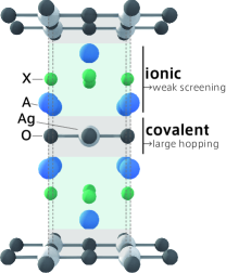
Figure 1: (Color online) Crystal structure of $A_{2}$AgO${}_{2}X_{2}$ ($A=$Sr and Ba, $X$=F, Cl, Br, and I), which belongs to T’-type structure studied in this paper.

Figure 2: (Color online) (a) La₂CuO₄-type (T-type) structure. (b) Nd₂CuO₄-type (T’-type) structure.

Figure 3: (Color online) Position of the $d_{x^{2}-y^{2}}$ and O $2p$ orbitals and definition of the $2\times 2$ sublattice used in the VMC for the three-band Hamiltonian. Phases of the orbitals are distinguished by yellow ($+$) and blue ($-$) colors.

In this paper we propose several silver as well as gold oxide compounds illustrated by typical crystal structure in Fig. 1 and derive their ab initio effective Hamiltonians after structural optimization and confirmation of the material stability to be used to predict electronic properties including correlation effects and superconductivity. To show its promising feature, we supplement with an attempt to solve one of the Hamiltonians for Sr₂AgO₂F₂, which has the largest Coulomb interaction relative to the nearest-neighbor transfer integral, by using a quantum many-body solver based on the variational Monte Carlo (VMC) method. It indeed shows that the mother compound has an antiferromagnetic Mott insulating ground state competing with a correlated metallic state. The structures we study is essentially T-type and T’-type layered perovskite structure illustrated in Figs. 2(a) and (b). The common lattice structure consisting of the transition metal $d$ and oxygen $p$ orbitals in our compounds are sketched in Fig. 3.

The organization of the paper is the following: In Sec. II, we briefly describe our ab initio method and computational conditions. We then propose our strategy of materials design to find promising strongly correlated systems that are distinct from the cuprates in Sec. III. In Sec. IV, the procedure of deriving Hamiltonians and the obtained effective Hamiltonians are presented for $A_{2}$AgO${}_{2}X_{2}$, and $A_{2}$AuO${}_{2}X_{2}$, where $A=$Sr and Ba, and $X=$F, Cl, Br, and I after structural optimization. A preliminary result of the VMC calculation for Sr₂AgO₂F₂ using the derived Hamiltonian is also shown in Sec. IV as a test case, which shows a rich and promising feature. Details of the VMC results will be reported elsewhere. Section V is devoted to concluding remark.

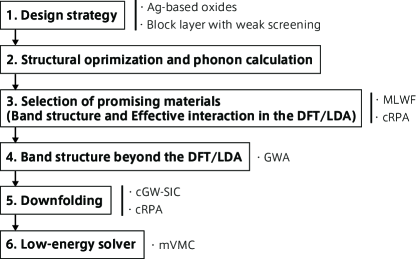
Figure 4: (Color online) Overview of material design scheme for strongly correlated systems in this paper. We focus on Ag- and Au-based compounds. MLWF, cRPA, GWA, cGW-SIC, and mVMC stand for maximally localized Wannier function, constrained random phase approximation, GW approximation, constrained GW approximation supplemented by the self-interaction correction, and many-variable variational Monte Carlo, respectively. See Sec. II for the details.

II Method

Strongly correlated electron systems have been a challenging field for theoretical understanding for decadesimada1998RMP . In particular, density functional calculation widely applied to predict electronic properties does not offer a satisfactory scheme because of the failure of representing strong correlation phenomena such as the Mott insulator imada1998RMP . To overcome the difficulty, by taking account of the universal hierarchical nature of the strongly correlated systems, which necessarily consist of the sparse and simple bands near the Fermi level, an efficient scheme based on the spirit of the renormalization group has been developed to derive effective Hamiltonians for such low-energy simple bands called the “target bands”. We apply this multi-scale ab initio scheme for correlated electrons (MACE) imadamiyake10 to derive low-energy effective Hamiltonian for the purpose of enabling the next step at which the derived Hamiltonian is solved by accurate quantum many-body solvers and to quantitatively predict physical quantities including superconductivity. This procedure is embedded in the basic flow chart of our materials design sketched in Fig. 4.

In the first step, we design the structure of the Ag- and Au-based oxides in terms of energy scales and feasible stability of the crystal structure. Next, we perform structural optimization for the candidate materials and calculate the phonon spectra to see the stability of the structure. By using the optimized structure, we derive the electronic effective Hamiltonian for the degrees of freedom near the Fermi level. We derive three-band Hamiltonians called $dpp$ Hamiltonian consisting of Ag 4$d_{x^{2}-y^{2}}$ (or Au 5$d_{x^{2}-y^{2}}$) and two O 2$p$ orbitals as well as one-band Hamiltonian for the antibonding band of these three orbitals. The forms of the effective Hamiltonians themselves already allow us to infer the correlation effect within the scope of this paper by comparing the ab initio Hamiltonian parameters with those of other existing materials such as the cuprates, which were already derived in a few compounds hirayama18 ; hirayama19 . We also supplement our proposal by solving the derived Hamiltonian by the VMC method, which indeed shows antiferromagnetic insulating phase for the mother compound, but with smaller Mott gap than the cuprates, which anticipates intriguing properties upon carrier doping. The VMC method is summarized in Appendix A.3.

II.1 Downfolding method

In this subsection, we briefly summarize the method of deriving the effective Hamiltonian by taking partial trace summation of the high-energy degrees of freedom far from the Fermi level. See Refs. hirayama18, and hirayama19, for detailed procedure. The effective Hamiltonian in the low-energy space (target space) is given in the form of extended Hubbard-type Hamiltonian without any adjustable parameters as

$$\mathcal{H}_{\text{eff}}^{\text{cGW-SIC}}=\sum_{ij}\sum_{\ell_{1}\ell_{2}\sigma} t^{\text{cGW-SIC}}_{\ell_{1}\ell_{2}\sigma}(\bm{R}_{i}-\bm{R}_{j})d_{i\ell_{1}\sigma}^{\dagger}d_{j\ell_{2}\sigma}$$

$$+\frac{1}{2}\sum_{i_{1}i_{2}i_{3}i_{4}}\sum_{{\color[rgb]{0,0,0}\ell_{1}\ell_{2}\ell_{3}\ell_{4}}\sigma\eta\rho\tau} \biggl{\{} W_{\ell_{1}\ell_{2}\ell_{3}\ell_{4}\sigma\eta\rho\tau}^{r}(\bm{R}_{i_{1}},\bm{R}_{i_{2}},\bm{R}_{i_{3}},\bm{R}_{i_{4}})$$ (1)

$$d_{i_{1}\ell_{1}\sigma}^{\dagger}d_{i_{2}\ell_{2}\eta}d_{i_{3}\ell_{3}\rho}^{\dagger}d_{i_{4}\ell_{4}\tau}\biggl{\}},$$

where $d_{i\ell\sigma}^{\dagger}$ ($d_{i\ell\sigma}$) is the creation (annihilation) operator of an electron for the $\ell$th maximally localized Wannier function (MLWF) with spin $\sigma$ centered at unit cell $\bm{R}_{i}$. Here, the single-particle term

$$t^{\text{cGW-SIC}}_{\ell_{1}\ell_{2}\sigma}(\bm{R})=\langle\phi_{\ell_{1}\bm{0}}|{H}^{\text{cGW-SIC}}_{K}|\phi_{\ell_{2}\bm{R}}\rangle,$$ (2)

and the interaction term

$$W_{\ell_{1}\ell_{2}\ell_{3}\ell_{4}\sigma\eta\rho\tau}^{r}(\bm{R}_{i_{1}},\bm{R}_{i_{2}},\bm{R}_{i_{3}},\bm{R}_{i_{4}})$$

$$=\langle\phi_{\ell_{1}\bm{R}_{i_{1}}}\phi_{\ell_{2}\bm{R}_{i_{2}}}|{H}^{\text{cGW-SIC}}_{W^{r}}|\phi_{\ell_{3}\bm{R}_{i_{3}}}\phi_{\ell_{4}\bm{R}_{i_{4}}}\rangle,$$ (3)

will be derived in this paper, where $\phi_{\ell\bm{R}_{i}}$ is the $\ell$th MLWF centered at $\bm{R}_{i}$. Following Refs. hirayama18, and hirayama19, , the one-body term (2) and the two-body term (3) were calculated by the constrained GW approximation (cGW) with the self-interaction correction (SIC)  hirayama13 and the constrained random phase approximation (cRPA) aryasetiawan04 , respectively, using the Green’s function of the band structure of all degrees of freedom. It should be noted that all the parameters in Eq.(1), namely $t^{\text{cGW-SIC}}$ and $W^{r}$, are given from the first principles calculation without any adjustable parameters.

In the later presentation, we often use the notation $U(0,0,0)$ or $U$, $V(l,m,n)$ and $t(l,m,n)$ for important parameters. These denote $(\ell_{1},\ell_{2})$ component of onsite interaction matrix $U_{\ell_{1},\ell_{2}}=W^{r}_{\ell_{1},\ell_{1},\ell_{2},\ell_{2},\sigma_{1},\sigma_{1},\sigma_{2},\sigma_{2},}(\bm{R}_{0},\bm{R}_{0},\bm{R}_{0},\bm{R}_{0})$, intersite Coulomb repulsion matrix $V_{\ell_{1},\ell_{2}}(l,m,n)=W^{r}_{\ell_{1},\ell_{1},\ell_{2},\ell_{2},\sigma_{1},\sigma_{1},\sigma_{2},\sigma_{2},}(\bm{R}_{0},\bm{R}_{0},\bm{R}_{0}+\bm{R},\bm{R}_{0}+\bm{R})$ and transfer $t_{\ell_{1},\ell_{2}}(l,m,n)=t_{\ell_{1},\ell_{2},\sigma}(\bm{R})$ where $\bm{R}=(l,m,n)$ in the length unit of the unitcell.

In this research, we follow the basic strategy of MACE. We first derive effective Hamiltonians based on the local density approximation (LDA) of the density functional theory (DFT) to capture the over all trend and to save the computational load. However, we next follow the same way as Refs. hirayama18, and hirayama19, and use the whole band structure obtained by the GW approximation (GWA) beyond the DFT/LDA to derive the most elaborated ab initio Hamiltonian for some Ag compounds.

In the cGWhirayama13 ; hirayama17 , the band dispersion is determined from the self-energy and the polarization by excluding the contribution from the low-energy degrees of freedom to remove the double counting; The cGW method can explicitly exclude the double counting of the exchange correlation energy in the effective Hamiltonian.

In this paper, we further take into account the chemical potential correction to make the orbital filling fixed at the GW result by following Ref. hirayama19, . For details of the method see Ref. hirayama19, . On the computational conditions related to phonon, DFT and GW, and VMC calculations, see Appendix A.

III Design strategy of ${\bf Ag}$-based superconductors

An important quantity throughout this paper is the effective correlation strength $|U/t|$ characterized by the ratio of the effective onsite interaction $U$ and the hopping amplitude $t$ between the nearest neighbor orbitals in the one-band effective Hamiltonian, which we will derive below. The intersite interaction $V_{1}$ (for the nearest neighbor) and $V_{2}$ (for the next nearest neighbor) relative to $U$ will also turn out to be important. Here, we summarize our idea of materials design in this paper by referring to these parameters. We propose a new silver compound with (AgO₂)^-2 plane as candidates showing promising feature by using the ab initio method.

Ag has an electronegativity closer to that of O than to that of Cu. Therefore, Ag and O in the AgO₂ plane would form a strong covalent bond and would have a larger energy scale hopping than in the case of the CuO₂ plane. However, the bare Coulomb interaction of the Ag $4d$ orbital is anticipated to be weaker than that of the Cu $3d$ orbital, and the correlation of the Ag-based system becomes weaker.

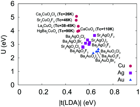
Figure 5: (Color online) Layered perovskites with Cu, Ag and Au are placed in the parameter plane of the nearest neighbor hopping $t$ in the LDA level and the on-site effective interaction $U$ for the single-band Hamiltonian in the Cu-, Ag-, and Au-based superconductors calculated by the cRPA method from the DFT band structures, which corresponds to the calculation in Section IV. B. Plots of Ag and Au compounds are one of the main results in the present paper.

As shown in Fig. 5, it is observed that the smaller the $U$ value (or equally $|U/t|$ because $t$ is similar), the higher the $T_{c}$ tends to be for the known copper oxides. This trend is consistent with our former analyses that too strong $|U/t|$ generates too strong effective attraction of carriers, which eventually results in the charge inhomogeneity instead of the superconductivity misawaHubbard ; misawainterface ; imada_suzuki ; imadareview21 . We note that this trend is opposite to the observation in the literature nilsson . In fact, it was pointed out that larger $|U/t|$ tends to show higher $T_{c}$ in the comparison of Bi₂Sr₂CuO₆, Bi₂Sr₂CaCuO₈, HgBa₂CuO₄ and CaCuO₂ Moree2022 . This implies that there exists the optimum value of $|U/t|$ to maximize $T_{c}$. In addition, it was shown that the off-site interactions have substantial effects on the amplitude of the superconducting order parameter. The amplitude also quantitatively depends on the detailed band structure. Therefore, it is desired to further cultivate variety in different family of compounds by materials design to reach comprehensive and quantitative understanding of the superconductivity, which also contributes to identify the superconducting mechanism.

Since Ag has a smaller bare interaction than the cuprates as we will show later, it offers an unprecedented approach from the weaker correlation side to reach the optimum: We try to enlarge the correlation effect of Ag-based compounds by designing the block layer to make weak screening to reach the optimum correlation and to achieve high $T_{c}$. Block layers containing halogens fit for this purpose by suppressing the screening: The closed $p$-orbital band of halogen is stable and appears far from the Fermi level, so the screening is expected to be weaker. In fact, the halogen system of copper oxides has a large $U$ as we will show later.

Halogens are also useful in terms of the valence of Ag. Ag is less likely to have an oxidation number greater than $+1$, which is smaller than Cu. However, by using a strong anion such as fluorine, it is possible to obtain a valence other than $+1$. For example, Ag in Cs₂AgF₄ is a divalent anion and has the same La₂CuO₄ structure (T structure) as K₂CuF₄.

In this paper, we consider $A_{2}$AgO${}_{2}X_{2}$ (A=Ca,Sr,Ba, X=F,Cl,Br,I) with T and T’ structures. These Ag compounds have not been reported in experiments yet. However, there exist similar mixed-anion systems Kageyama2018 in case of copper such as Ca₂CuO₂Cl₂ and Sr₂CuO₂F₂ and palladium such as Ba₂PdO₂F₂ and Ba₂PdO₂Cl₂. We also calculate Au-based oxides with a similar block layer for comparison. The Au-based oxide is expected to have an even smaller correlation than that of Ag.

IV Result

We here present the ab initio low-energy Hamiltonians for $A_{2}$AgO${}_{2}X_{2}$ and $A_{2}$AuO${}_{2}X_{2}$ with $A=$Sr and Ba and $X=$F, Cl, Br and I. We also discuss basic properties for Sr₂AgO₂F₂ by solving the ab initio Hamiltonian using the mVMC.

IV.1 Dynamical stability

Table 1: Structural parameters of the studied T’-type $A_{2}$AgO${}_{2}X_{2}$ (space group: $I4/mmm$) optimized with PBEsol functional. The $A$ atoms occupy the 4e Wyckoff site $(0,0,\pm z_{A})$. The Ag, O, and $X$ atoms are located at the 2a, 4c, and 4d sites, respectively.

Composition	$a$ (Å)	$c$ (Å)	$c/a$	$z_{A}$
Sr2AgO2F2	4.146	12.428	2.9974	0.3632
Sr2AgO2Cl2	4.359	14.083	3.2306	0.3844
Sr2AgO2Br2	4.439	14.759	3.3247	0.3942
Sr2AgO2I2	4.585	15.670	3.4174	0.4056
Ba2AgO2F2	4.268	13.668	3.2028	0.3649
Ba2AgO2Cl2	4.467	15.254	3.4145	0.3857
Ba2AgO2Br2	4.536	15.854	3.4952	0.3947
Ba2AgO2I2	4.665	16.627	3.5640	0.4047

Table 2: Structural parameters of the studied T-type $A_{2}$AgO${}_{2}X_{2}$ (space group: $I4/mmm$) optimized with PBEsol functional. The $A$ and $X$ atoms occupy the 4e site $(0,0,\pm z)$, and Ag atoms and O atoms are located at the 2a and 4c sites, respectively.

Composition	$a$ (Å)	$c$ (Å)	$c/a$	$z_{A}$	$z_{X}$
Sr2AgO2F2	4.093	13.293	3.248	0.3749	0.1970
Sr2AgO2Cl2	4.155	15.245	3.669	0.3900	0.1884
Sr2AgO2Br2	4.184	16.245	3.883	0.3974	0.1851
Sr2AgO2I2	4.215	18.489	4.386	0.4116	0.1760
Ba2AgO2F2	4.145	14.323	3.455	0.3721	0.1895
Ba2AgO2Cl2	4.258	16.148	3.792	0.3878	0.1857
Ba2AgO2Br2	4.303	16.932	3.935	0.3941	0.1852
Ba2AgO2I2	4.359	18.478	4.240	0.4050	0.1821

The structural parameters of the designed Ag-based oxides optimized by using the PBEsol functional are summarized in Tables 1 and 2. As is shown in Fig. 1, two halogen ions in the T’-type structure are located in the same $X_{2}$ plane, whereas they are in different but adjacent planes in the T-type structure, where T and T’ structures are illustrated in Fig. 2. Hence, the in-plane (out-of-plane) lattice constant of the T’-type structure becomes larger (smaller) than that of the T-type. The relative stability of the two structures is also evaluated from the difference of the ground state energy; the T’-type structure is energetically more stable than the T-type only for $X=$ F, whereas the T-type is preferable for larger halogen ions ($X=$ Cl, Br, and I). This tendency is consistent with the experimental findings on the isostructural Cu oxides; Sr₂CuO₂F₂ displays the T’-type structure Kissick , while Sr₂CuO₂Cl₂ crystallizes in the T-type Miller . The same tendency was also reported in a recent theoretical study of nickel oxides Hirayama_materials_design_prb2020 .

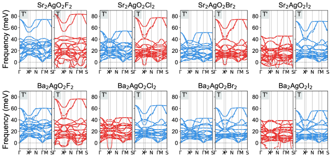
Figure 6: Phonon dispersion of the Ag-based oxides computed within harmonic approximation. The solid lines are results obtained using the 2$\times$2$\times$2 supercell, and the dashed lines represent the result obtained using a larger supercell containing 112 atoms. The imaginary frequencies are shown as negative values. Different colors are used for dynamically stable (blue) and unstable (red) systems.

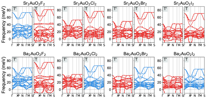
Figure 7: Phonon dispersion of the Au-based oxides computed within harmonic approximation. The meaning of the different line styles and colors are described in Fig. 6 caption.

Figure 6 compares the calculated phonon dispersion curves of the T’- and T-type Ag-based oxides $A_{2}$AgO${}_{2}X_{2}$. Among the 16 Ag-based oxides, nine oxides are predicted to be dynamically stable, which are shown with blue lines in Fig. 6. For $X$=F, the T’-type structure is dynamically stable, whereas the T-type is dynamically unstable where imaginary phonon modes appear in the wide-range of the Brillouin zone (BZ). In the largest halogen ion case ($X$=I), the T-type is dynamically stable and the T’-type is unstable. This $X$-dependency of the dynamical stability is consistent with the energy difference between the T-type and T’-type phases mentioned above. For Sr₂AgO₂Cl₂ and Sr₂AgO₂Br₂, the T-type phase appears to be dynamically unstable even though it is energetically more stable than the T’-type structure. The soft phonon mode of the T-type phases, which appears only around the X and P points of the BZ, involves in-plane displacements of the corner-sharing oxygen atoms in the AgO₂ plane and induces the structural phase transition to a lower-symmetry orthorhombic phase, which resembles the unstable octahedral tilting mode in the tetragonal (T-type) La₂CuO₄ LCO_phonon . Since the distortion of the tetragonal La₂CuO₄ to the orthorhombic phase can be suppressed by hole doping LCO_hole_doping , a similar doping approach is expected to improve the stability of the T-type Sr₂AgO₂Cl₂ and Sr₂AgO₂Br₂. For $A=$ Ba, the $X$-dependency of the dynamical stability is similar to the case of $A=$ Sr except for $X=$ Cl and Br where the T-type is predicted to be dynamically stable. The soft phonons observed in the T-type Sr₂AgO${}_{2}X_{2}$ ($X=$ Cl, Br) are stabilized in the corresponding Ba₂AgO${}_{2}X_{2}$, which can be attributed to the larger in-plane lattice constants of the Ba systems along with the negative Grüneisen parameter of the soft mode.

For the Au-based oxide, the halogen-ion dependency of the lattice parameters, energy difference between the T’- and T-type structures, and the dynamical stability are the same as the Ag-based oxides, as shown in Tables  3 and  4 in Appendix  B and Fig. 7. However, only five structures are predicted to be dynamically stable.

Table 3: Structural parameters of the studied T’-type $A_{2}$AuO${}_{2}X_{2}$ (space group: $I4/mmm$) optimized with PBEsol functional. The $A$ atoms occupy the 4e Wyckoff site $(0,0,\pm z_{A})$. The Au, O, and $X$ atoms are located at the 2a, 4c, and 4d sites, respectively.

Composition	$a$ (Å)	$c$ (Å)	$c/a$	$z$
Sr2AuO2F2	4.173	12.435	2.9802	0.3616
Sr2AuO2Cl2	4.363	14.115	3.2352	0.3823
Sr2AuO2Br2	4.445	14.760	3.3203	0.3920
Sr2AuO2I2	4.587	15.691	3.4208	0.4043
Ba2AuO2F2	4.276	13.707	3.2055	0.3639
Ba2AuO2Cl2	4.456	15.327	3.4396	0.3843
Ba2AuO2Br2	4.534	15.845	3.4944	0.3923
Ba2AuO2I2	4.656	16.688	3.5845	0.4042

Table 4: Structural parameters of the studied T-type $A_{2}$AuO${}_{2}X_{2}$ (space group: $I4/mmm$) optimized with PBEsol functional. The $A$ and $X$ atoms occupy the 4e site $(0,0,\pm z)$, and Au atoms and O atoms are located at the 2a and 4c sites, respectively.

Composition	$a$ (Å)	$c$ (Å)	$c/a$	$z_{A}$	$z_{B}$
Sr2AuO2F2	4.126	13.558	3.286	0.3744	0.2022
Sr2AuO2Cl2	4.175	15.474	3.707	0.3889	0.1918
Sr2AuO2Br2	4.201	16.413	3.907	0.3960	0.1880
Sr2AuO2I2	4.231	18.573	4.390	0.4102	0.1783
Ba2AuO2F2	4.165	14.580	3.501	0.3716	0.1947
Ba2AuO2Cl2	4.256	16.409	3.856	0.3870	0.1891
Ba2AuO2Br2	4.296	17.177	3.999	0.3933	0.1878
Ba2AuO2I2	4.350	18.663	4.290	0.4041	0.1840

IV.2 Selection of promising materials

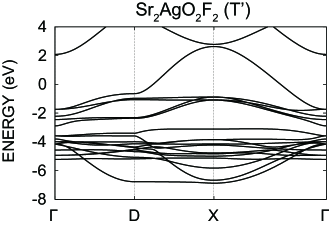
Figure 8: (Color online) Electronic band structure of Sr₂AgO₂F₂ in the LDA. The zero energy corresponds to the Fermi level.

For all stable Ag- and Au-based oxides and the representative Cu-based oxides, we perform the band structure calculations in the DFT/LDA. Figure 8 shows a LDA band structure of one of them, for Sr₂AgO₂F₂. As in the case of typical cuprates, a single band originating from the antibonding orbitals appears on the Fermi level in all the Ag- and Au-based oxides calculated in this study. Therefore, as in the case of the copper oxides, it is possible to discuss the system in terms of a low-energy effective Hamiltonian consisting mainly of an antibonding orbital.

Table 5: On-site potentials and effective interactions for one-band Hamiltonian of Cu-, Ag-, and Au-based compounds (in eV). The one-body part is obtained from the fitting of the LDA band structure, while the effective interaction is the result of the cRPA from the LDA bands. $v$, $U$, and $V$ represent the bare Coulomb, the static values of the effective on-site Coulomb, and the effective off-site Coulomb, respectively (at $\omega=0$). $U/v$ is the ratio of the on-site bare and screened Coulomb interactions, and $U/t$ is the ratio of the nearest neighbor hopping and the screened Coulomb interaction.

Cu	$t(1,0,0)$	$t(1,1,0)$	$t(2,0,0)$	$v(0,0,0)$	$U(0,0,0)$	$v(1,0,0)$	$V(1,0,0)$	$v(1,1,0)$	$V(1,1,0)$	$v(2,0,0)$	$V(2,0,0)$	$U/v$	$|U/t|$
Ca2CuO2Cl2	-0.492	0.091	-0.053	18.220	5.063	4.170	1.183	2.768	0.736	2.090	0.534	0.278	10.29
La2CuO4	-0.507	0.084	-0.051	18.354	4.335	4.241	0.665	2.825	0.345	2.138	0.231	0.236	8.55
Sr2CuO2F2	-0.489	0.105	-0.049	18.449	4.780	4.088	0.962	2.699	0.542	2.033	0.361	0.259	9.78
HgBa2CuO4	-0.502	0.091	-0.063	16.856	3.957	4.164	0.763	2.749	0.407	2.090	0.270	0.235	7.88
CaCuO2	-0.512	0.084	-0.062	17.104	3.999	4.193	0.763	2.758	0.361	2.081	0.204	0.234	7.81
Ag	$t(1,0,0)$	$t(1,1,0)$	$t(2,0,0)$	$v(0,0,0)$	$U(0,0,0)$	$v(1,0,0)$	$V(1,0,0)$	$v(1,1,0)$	$V(1,1,0)$	$v(2,0,0)$	$V(2,0,0)$	$U/v$	$|U/t|$
Sr2AgO2F2 (T’)	-0.644	0.111	-0.120	11.046	3.653	3.974	1.239	2.607	0.773	1.983	0.590	0.331	5.67
Sr2AgO2Cl2 (T’)	-0.545	0.094	-0.114	10.310	2.813	3.802	0.730	2.487	0.346	1.900	0.227	0.273	5.16
Sr2AgO2I2 (T)	-0.602	0.103	-0.106	10.988	3.132	3.904	0.790	2.566	0.404	1.952	0.278	0.285	5.20
Ba2AgO2F2 (T’)	-0.596	0.106	-0.119	10.468	2.999	3.873	0.875	2.537	0.473	1.936	0.332	0.286	5.03
Ba2AgO2Cl2 (T)	-0.585	0.099	-0.110	10.675	3.323	3.871	1.078	2.542	0.667	1.939	0.511	0.311	5.68
Ba2AgO2Br2 (T)	-0.568	0.100	-0.109	10.512	3.080	3.833	0.905	2.516	0.511	1.922	0.369	0.293	5.42
Ba2AgO2I2 (T)	-0.547	0.100	-0.109	10.316	2.780	3.788	0.699	2.485	0.340	1.901	0.225	0.269	5.08
Au	$t(1,0,0)$	$t(1,1,0)$	$t(2,0,0)$	$v(0,0,0)$	$U(0,0,0)$	$v(1,0,0)$	$V(1,0,0)$	$v(1,1,0)$	$V(1,1,0)$	$v(2,0,0)$	$V(2,0,0)$	$U/v$	$|U/t|$
Ba2AuO2F2 (T’)	-0.674	0.166	-0.151	9.230	2.474	3.838	0.758	2.535	0.433	1.987	0.342	0.268	3.67
Ba2AuO2Cl2 (T)	-0.676	0.162	-0.141	9.436	2.634	3.843	0.815	2.551	0.467	1.987	0.342	0.279	3.90
Ba2AuO2Br2 (T)	-0.659	0.160	-0.141	9.319	2.454	3.809	0.689	2.527	0.366	1.975	0.274	0.263	3.72
Ba2AuO2I2 (T)	-0.633	0.158	-0.138	9.221	2.338	3.763	0.596	2.496	0.282	1.954	0.199	0.254	3.69

From the obtained band structure, following the standard MACE procedure, we construct one-band Hamiltonians of the antibonding orbital and three-band Hamiltonians of the $x^{2}-y^{2}$ and the $2p$ orbitals first on the LDA level to quickly pick up promising candidates to be examined later in depth. We summarize thus obtained results of the most important parameters of the effective one-band Hamiltonian in Table 5.

See also Appendix C for the corresponding Wannier function and for the fitting of one band for several other Ag-based oxides. In the antibonding Wannier function, the $x^{2}-y^{2}$ orbital of Ag and the $2p$ orbitals of O are strongly hybridized. Therefore, the bandwidth of the antibonding band is very large, 5-6 eV.

Here, we focus on the effective correlation strength $|U/t|$ listed up in Table 5. Note that $U/t$ here is obtained from a simple fitting of the LDA band together with the cRPA, where $U$ is derived from the LDA band and $t$ is a simple fitting of the LDA band. More precise estimates of $U$ and $t$ for several Ag-based oxides will be given later. It is known hirayama18 ; hirayama19 that the copper oxides have large $|U/t|$ of 8-10, and systems with smaller $|U/t|$ tend to have higher $T_{c}$. HgBa₂CuO₄ and CaCuO₂ exhibiting relatively high $T_{c}$ indeed have $|U/t|\sim 8$, which are near the lower boundary of the cuprates and it is desired to find lower $|U/t|$ to seek for higher $T_{c}$ by considering the possibility that the cuprates did not reach the optimized $U/t$.

For the Ag-based oxides we selected, however, $|U/t|$ is about 5-6. Compared to the copper oxides, it provides us with an approach from relatively weaker correlation side. The nearest-neighbor hopping of cuprate is about $-0.50$ eV, regardless of the compounds. On the other hand, the silver oxides have larger hopping amplitudes than that of the copper oxides. The hopping of silver oxide strongly depends on the materials, ranging from $-0.65$ eV to $-0.55$ eV, and has larger value roughly for smaller lattice constant (see Tables 1 and 2). Of course, larger $|t|$ is preferred to make the characteristic energy scale and the resultant possible superconducting gap and temperature scales higher. We have also calculated the Au-based oxide for comparison. The $|U/t|$ is about 3.5-4 and the system is not strongly correlated.

From these analyses, we pick up compounds that have either larger $|U/t|$ or larger $|t|$: Below we study in depth four Ag-based oxides, Sr₂AgO₂F₂, Sr₂AgO₂I₂, Ba₂AgO₂F₂, and Ba₂AgO₂Cl₂ for more detailed and accurate studies with heavier computational cost. The choice of four compounds is also supported from the analyses in Appendix C for the three band Hamiltonian on the LDA level.

IV.3 Effective Hamiltonian derived at the cGW-SIC beyond the DFT/LDA level

Now, we present the effective Hamiltonians obtained by using more accurate procedure of MACE beyond DFT/LDA level. For a while, we focus on the Ag-based oxides and compare with the cuprates. We employ the standard procedure of the MACE imadamiyake10 ; hirayama17 ; hirayama18 ; hirayama19 . In the cGW-SIC scheme, we first replace the LDA with the GWA, which enables us more accurate calculation of the correlation effect of the bands outside of the low-energy Hamiltonian than the LDA. It also enables removing the double counting of the correlation effect in the effective Hamiltonian, which is unavoidable when we rely on the LDA. Figure 17 in Appendix D shows the band structures obtained in the GWA which is used in the next step of the cGW-SIC. The effective Hamiltonian at the GW level as the intermediate step is described in Appendix D.

The final and most accurate effective Hamiltonian is given in the cGW-SIC level by using the GW band structure obtained above as the starting point and we present one-band Hamiltonian for the antibonding band and the three-band Hamiltonian as well by using the two bases: One, basis of both $d_{x^{2}-y^{2}}$ and two $2p$ orbitals ($dpp$ basis) and the other, the basis in the antibonding and two bonding orbitals (abb basis).

IV.3.1 Derivation of single-band Hamiltonian

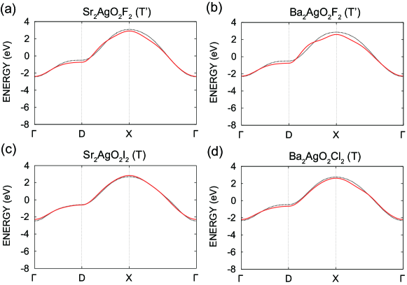
Figure 9: (Color online) Electronic band structure of one-band Hamiltonian in the cGW originating from the anti-bonding Wannier orbitals. The zero energy corresponds to the Fermi level. For comparison, the fitting band structure for the GWA is also given (black dotted line).

First, as in the LDA calculations, we summarize the parameters of the one-band Hamiltonian at the cGW level, by using the hopping calculated from the maximally localized Wannier orbitals constructed from the GW band and the effective interaction obtained by the cRPA, in Table 6 for the four Ag compounds LR . We summarize the details of the one-band parameters in Supplemental Materials smdata . Figure 9 shows the corresponding band structure at the cGW level. The $|U/t|$ values are larger than that in the LDA due to the self-energy effect, with the largest value being about 6.69 in Sr₂AgO₂F₂, which is larger than the simplified derivation 5.67 in Table 5. The nearest-neighbor hopping of Sr₂AgO₂F₂ is also $-0.708$ eV, which is larger than that in the LDA fitting $-0.644$ eV, and the energy scale is increased.

Table 6: Transfer integral and effective interaction in one-band Hamiltonian for Sr₂AgO₂F₂, Sr₂AgO₂I₂, Ba₂AgO₂F₂, and Ba₂AgO₂Cl₂ (in eV). Transfer integrals and effective interactions are obtained by using the cGW and the cRPA applied to the GW Green’s function, respectively. $v$, $U$, and $V$ represent the bare Coulomb, the static values of the effective on-site Coulomb, and the effective off-site Coulomb, respectively (at $\omega=0$). The parameters for further neighbor transfer integrals and interactions by the cGW are given in Table 15 for Sr₂AgO₂F₂ and for other compounds, in the Supplemental Material smdata .

cGW	$t(1,0,0)$	$t(1,1,0)$	$t(2,0,0)$	$v(0,0,0)$	$U(0,0,0)$	$v(1,0,0)$	$V(1,0,0)$	$v(1,1,0)$	$V(1,1,0)$	$v(2,0,0)$	$V(2,0,0)$	$U/v$	$|U/t|$
Sr2AgO2F2 (T’)	-0.658	0.092	-0.101	11.964	4.401	3.982	1.464	2.603	0.966	1.961	0.771	0.368	6.69
Ba2AgO2F2 (T’)	-0.609	0.067	-0.093	11.485	4.010	3.894	1.282	2.533	0.811	1.911	0.629	0.349	6.58
Sr2AgO2I2 (T)	-0.626	0.101	-0.093	11.063	3.337	3.907	0.938	2.564	0.535	1.951	0.393	0.302	5.33
Ba2AgO2Cl2 (T)	-0.589	0.093	-0.099	11.434	3.728	3.881	1.115	2.536	0.694	1.914	0.535	0.326	6.33

IV.3.2 Derivation of three-band $dpp$ Hamiltonian

Table 7: Transfer integrals and effective interactions for three-band $dpp$ Hamiltonian of Sr₂AgO₂F₂ (T’) (in eV). We show the transfer integral in the cGW-SIC, while the effective interaction is the result of the cRPA. $v$ and $J_{v}$ represent the bare Coulomb and exchange interactions, respectively. $U$, $V$, and $J$ represent the static values of the on-site effective Coulomb, the off-site effective Coulomb, and exchange interactions, respectively (at $\omega=0$). The occupation number in the GWA is also given in the bottom column “occu.(GWA)” in this Table. The parameters for further neighbor transfer integrals and interactions by the cGW-SIC are given in the Supplemental Material smdata .

cGW-SIC		$t(0,0,0)$			$t(1,0,0)$			$t(1,1,0)$			$(2,0,0)$
	$x^{2}-y^{2}$	$p_{1}$	$p_{2}$	$x^{2}-y^{2}$	$p_{1}$	$p_{2}$	$x^{2}-y^{2}$	$p_{1}$	$p_{2}$	$x^{2}-y^{2}$	$p_{1}$	$p_{2}$
$x^{2}-y^{2}$	-3.091	-1.562	1.562	-0.003	-0.059	-0.070	0.028	-0.015	0.015	-0.023	0.008	-0.003
$p_{1}$	-1.562	-3.702	-0.688	1.562	0.288	0.688	-0.070	0.061	0.011	0.059	-0.019	0.011
$p_{2}$	1.562	-0.688	-3.702	-0.070	-0.011	-0.060	0.070	0.011	0.061	-0.003	0.002	0.000
		$v(0,0,0)$			$U(0,0,0)$			$J_{v}(0,0,0)$			$J(0,0,0)$
	$x^{2}-y^{2}$	$p_{1}$	$p_{2}$	$x^{2}-y^{2}$	$p_{1}$	$p_{2}$	$x^{2}-y^{2}$	$p_{1}$	$p_{2}$	$x^{2}-y^{2}$	$p_{1}$	$p_{2}$
$x^{2}-y^{2}$	19.455	7.519	7.519	8.493	2.865	2.865		0.084	0.084		0.064	0.064
$p_{1}$	7.519	17.012	5.030	2.865	6.213	1.891	0.084		0.043	0.064		0.020
$p_{2}$	7.519	5.030	17.012	2.865	1.891	6.213	0.084	0.043		0.064	0.020
		$v(1,0,0)$			$V(1,0,0)$			$v(1,1,0)$			$V(1,1,0)$
	$x^{2}-y^{2}$	$p_{1}$	$p_{2}$	$x^{2}-y^{2}$	$p_{1}$	$p_{2}$	$x^{2}-y^{2}$	$p_{1}$	$p_{2}$	$x^{2}-y^{2}$	$p_{1}$	$p_{2}$
$x^{2}-y^{2}$	3.585	7.519	3.149	1.466	2.865	1.214	2.545	3.152	3.152	0.991	1.216	1.216
$p_{1}$	2.431	3.681	2.283	1.015	1.557	0.911	2.050	2.536	2.287	0.814	0.994	0.913
$p_{2}$	3.152	5.032	3.411	1.216	1.893	1.264	2.050	2.287	2.536	0.814	0.913	0.994
occ.(GWA)	$x^{2}-y^{2}$	$p_{1}$	$p_{2}$
	1.544	1.728	1.728

Table 8: Transfer integrals and effective interactions for three-band abb Hamiltonian of Sr₂AgO₂F₂ (T’) in the abb gauge (in eV). We show the transfer integral in the GW and the cGW-SIC, while the effective interaction is the result of the cRPA. The Wannier center of one antibonding and two bonding orbitals are the same as those of the $d$ and $p$ orbitals. $v$ and $J_{v}$ represent the bare Coulomb and exchange interactions, respectively. $U$, $V$, and $J$ represent the static values of the on-site effective Coulomb, the off-site effective Coulomb, and exchange interactions, respectively (at $\omega=0$). The occupation number in the GWA is also given in the bottom column “occu.(GWA)” in this Table.

GW		$t(0,0,0)$			$t(1,0,0)$			$t(1,1,0)$			$t(2,0,0)$
	$a$	$b_{1}$	$b_{2}$	$a$	$b_{1}$	$b_{2}$	$a$	$b_{1}$	$b_{2}$	$a$	$b_{1}$	$b_{2}$
$a$	0.102	0.000	0.000	-0.615	0.000	0.000	0.080	0.000	0.000	-0.130	0.000	0.000
$b_{1}$	0.000	-5.140	0.135	0.000	0.732	-0.136	0.000	0.006	-0.051	0.000	0.148	-0.051
$b_{2}$	0.000	0.135	-5.140	0.000	0.051	-0.009	0.000	-0.051	0.006	0.000	0.010	-0.020
cGW-SIC		$t(0,0,0)$			$t(1,0,0)$			$t(1,1,0)$			$t(2,0,0)$
	$a$	$b_{1}$	$b_{2}$	$a$	$b_{1}$	$b_{2}$	$a$	$b_{1}$	$b_{2}$	$a$	$b_{1}$	$b_{2}$
$a$	0.062	-0.055	-0.055	-0.631	-0.056	-0.024	0.141	0.002	-0.002	-0.192	-0.010	0.006
$b_{1}$	-0.055	-5.279	0.107	0.055	0.845	-0.107	-0.024	0.005	-0.054	0.056	0.164	-0.054
$b_{2}$	-0.055	0.107	-5.279	-0.024	0.054	0.011	0.024	-0.054	0.005	0.006	0.010	-0.013
		$v(0,0,0)$			$U(0,0,0)$			$J_{v}(0,0,0)$			$J(0,0,0)$
	$a$	$b_{1}$	$b_{2}$	$a$	$b_{1}$	$b_{2}$	$a$	$b_{1}$	$b_{2}$	$a$	$b_{1}$	$b_{2}$
$a$	10.045	7.571	7.571	4.088	2.928	2.928		1.738	1.738		0.703	0.703
$b_{1}$	7.571	12.902	5.095	2.928	4.924	1.944	1.738		0.153	0.703		0.072
$b_{2}$	7.571	5.095	12.902	2.928	1.944	4.924	1.738	0.153		0.703	0.072
		$v(1,0,0)$			$V(1,0,0)$			$v(1,1,0)$			$V(1,1,0)$
	$a$	$b_{1}$	$b_{2}$	$a$	$b_{1}$	$b_{2}$	$a$	$b_{1}$	$b_{2}$	$a$	$b_{1}$	$b_{2}$
$a$	3.976	7.571	3.193	1.540	2.928	1.231	2.604	3.196	3.196	1.013	1.233	1.233
$b_{1}$	2.730	4.422	2.347	1.115	1.821	0.937	2.105	2.550	2.351	0.834	0.999	0.939
$b_{2}$	3.196	5.097	3.259	1.233	1.946	1.228	2.105	2.351	2.550	0.834	0.939	0.999
occ.(GWA)	$a$	$b_{1}$	$b_{2}$
	1.000	2.000	2.000

We also present the three-band Hamiltonian using the cGW-SIC method. Unlike the one-body terms calculated by simple LDA, there are less drawbacks such as double counting of low-energy degrees of freedom. We summarize in Table 7 detailed three-band parameters of the effective Hamiltonian at the cGW-SIC level based on the Wannier basis of Cu $d$ and O $p$ basis for Sr₂AgO₂F₂ LR . We ignore the level renormalization taken into account before hirayama19 because its effect is small. We summarize the details of the three-band parameters in Supplemental Materials smdata . In Appendix E, we show comparison of the band dispersions and effective Hamiltonians of four Ag-based compounds.

IV.3.3 Derivation of three-band abb Hamiltonian

The three band Hamiltonian ($dpp$ Hamiltonian) represented in the $d$ and $p$ Wannier orbitals above can alternatively be represented by an antibonding orbital and two bonding orbitals. When calculating with the VMC method, it is better to transform the basis to such a basis, since the Gutzwiller factor introduces only diagonal terms, where the most important local interaction at the antibonding band is straightforwardly and efficiently taken into account. In this paper, we refer to this effective Hamiltonian as the abb Hamiltonian. In Table. 8, we show the GW and cGW-SIC parameters for the Sr₂AgO₂F₂ in the abb Hamiltonian. We also summarize the details of the three-band parameters in the abb-gauge in Supplemental Materials smdata . For the $dpp$ band in the GWA, we apply the method of the maximally localized Wannier function to each of the anti-bonding band and the other two bands, and get the Wannier function in the abb Hamiltonian. For hopping that reproduces the GW band, the anti-bonding orbital and the two bonding orbitals are orthogonal. In the cGW-SIC, however, the anti-bonding orbital and the two bonding orbitals are not strictly orthogonal, but the hoppings between them are small ($\sim$ 55 meV). We also note that the two bonding orbitals are not orthogonal even at the GW level, because the Wannier orbitals are constructed to satisfy the maximally localized nature, which means that the two bonding orbitals here is represented by the linear combination of the orthognal bonding and nonbonding states. Since the $d$ and $p$ orbitals form a strong covalent bond, the energy difference between the anti-bonding orbital and the two bonding orbitals is very large ($\sim$ 5 eV) due to the hybridization gap. Therefore, the screening effect from the bonding and nonbonding orbitals for the antibonding electrons, which have small hopping and large energy difference with the bonding/nonbonding states, would be small. The values of hopping and interaction of the antibonding orbital in the abb Hamiltonian are similar to the one-band Hamiltonian except for some reduction of the interaction and the modification of the longer ranged part of the hopping understood as the screening and the self-energy effects from the bonding/nonbonding electrons. The reason why we do not employ the basis that diagonalizes the cGW-SIC band instead of the GW band is that the GW band should express rather better overall electronic structure after considering the correlation of the three bands. Because of the large gap between the bonding and antibonding bands, the two bonding orbitals are nearly fully filled and only the antibonding band becomes partially filled, which makes the abb representation superior to the $dpp$ basis. This also means the single-band Hamiltonian is a good approximation and we solve it by the VMC below.

IV.4 Ground state of low-energy Hamiltonians

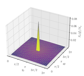
Figure 10: (Color online) Momentum dependence of spin structure factor $S_{s}(\bm{q})$ of non-doped Hamiltonian for Sr₂AgO₂F₂ calculated for a $24\times 24$ lattice.

Figure 11: (Color online) Momentum distribution $n(\bm{k})$ of non-doped Hamiltonian for Sr₂AgO₂F₂ calculated for a $24\times 24$ lattice.

Here we show a preliminary result of the ground state for the ab initio single-band effective Hamiltonian of Sr₂AgO₂F₂ on the cGW-SIC level obtained by VMC calculations to gain insight into Ag-based compounds whether our proposed materials show promising strong correlation effects. In the VMC calculation, we take into account the transfer integral up to the distance $(m,n)$ on the two-dimensional square lattice with $m,n\leq 3$. For the interaction, we also take into account in the same range but for $(3,n)$, we fit from the result of $(2,n)$ in the form $a/\sqrt{m^{2}+n^{2}}$ with a constant $a$ because the $1/r$ fitting is known to be satisfactory already at $(2,n)$ (see Appendix B of Ref. ohgoe20, ). In the solution obtained by the VMC calculation, two states are severely competing in the stoichiometric mother material, Sr₂AgO₂F₂; the G-type antiferromagnetic state with the normal staggered Neel order, and correlated paramagnetic metal. The true ground state is the antiferromagnetic state with the energy $E_{\rm AF}\sim$15.238 eV (per Ag site) in comparison to $E_{\rm metal}\sim$15.241 eV for the paramagnetic metal after the variance extrapolation for $24\times 24$ lattice. The ground state is indeed characterized by the Bragg peak at $\bm{Q}=(\pi,\pi)$ of the spin structure factor defined in Eq.(6) as is shown in Fig. 10. The ordered moment $m$ in Eq. (7) has a nonzero value $\sim 0.56$ slightly smaller than the case of La₂CuO₄hirayama19 . The momentum distribution defined in Eq. (8) for the antiferromagnetic ground state is given in Fig. 11 for the $24\times 24$ lattice, clearly indicating the insulating nature with the absence of the Fermi surface. Therefore, the mother material is characterized by the antiferromagnetic Mott insulator, which is similar to the cuprates. However, the metallic state is severely competing with the antiferromagnetic insulator in the present case due to relatively weak correlations.

V Concluding Remark

We have demonstrated that the present family of silver-based compounds potentially shows strong correlation effects similar to the cuprates. In the example of Sr₂AgO₂F₂, the non-doped mother compound shows the antiferromagnetic Mott insulating ground state with the ordered moment comparable to La₂CuO₄. It offers promising candidates of the superconductivity when carriers are doped.

It should be noted that Sr₂AgO₂F₂ has the largest off-site Coulomb interaction in the present family, while Sr₂AgO₂I₂ and Ba₂AgO₂Cl₂ have substantially weaker off-site interaction, which may enhance the superconductivity ohgoe20 though $|U/t|$ is slightly smaller. In this sense Ag compounds open possibility of controlling parameters that affect the competition between superconductivity and other states, which contributes to the comprehensive understanding of the correlation induced superconductivity. More thorough studies on the possible superconductivity will be reported elsewhere. It is desired to investigate this family of materials experimentally after confirming that these materials can really be synthesized in accordance with the present prediction.

Appendix A Computational Conditions

A.1 Conditions for phonon calculation

The cell parameters and internal coordinates of the Ag- and Au-based oxides are fully relaxed using the Vienna Ab initio Simulation Package (VASP) vasp , which implements the projector augmented wave (PAW) method paw ; paw2 . The VASP recommended PAW potentials for calculations based on the DFT are used together with the kinetic-energy cutoff of 500 eV for the plane wave expansion. The $k$-point mesh for the Brillouin zone integration is generated automatically so that the mesh density becomes as high as 450 $\mathrm{\AA}^{3}$. For the exchange-correlation potential, we employ the PBEsol functional within the generalized gradient approximation (GGA) pbesol , which gives better prediction accuracy of the structural parameters than GGA-PBE pbe and the LDA. The dynamical stability of each material is then accessed from the presence or absence of imaginary phonons in the phonon dispersion obtained within the harmonic approximation. To this end, we calculate phonon dispersion curves using the 2$\times$2$\times$2 supercells (containing 56 atoms) of the fully optimized structures using the finite displacement method, as implemented in the ALAMODE software alamode . If an unstable phonon, whose squared frequency is negative ($\omega_{\bm{q}\nu}^{2}<0$), is found on the commensurate 2$\times$2$\times$2 $\bm{q}$ points, the material is identified to be dynamically unstable; otherwise the system is dynamically stable. We further confirm the dynamical stability by using a larger supercell containing 112 atoms, which gives the quantitatively similar results as shown in Figs. 6 and 7.

A.2 Conditions for DFT and GW

We calculate the electronic structure of the Cu-based compound using the experimental lattice parameters. We employ the experimental results reported by Ref. Putilin, for HgBa₂CuO₄, those reported by Ref. Jorgensen, for La₂CuO₄, those reported by Ref. Hiroi, for Ca₂CuO₂Cl₂, those reported by Ref. Kissick, for Sr₂CuO₂F₂, and those reported by Ref. Karpinski, for CaCuO₂. We calculate the electronic structure of the Ag-based and Au-based compounds using the lattice constants obtained from the structural optimization.

Computational conditions for the DFT/LDA and GW are as follows. The band structure calculation is based on the full-potential linear muffin-tin orbital (LMTO) implementation methfessel . The exchange correlation functional is obtained by LDA of the Ceperley-Alder type. ceperley We neglect the spin-polarization. The self-consistent LDA calculation is done for the 12 $\times$ 12 $\times$ 12 $k$-mesh. The muffintin (MT) radii are as follows: $R^{\text{MT}}_{\text{Ca(Ca2CuO2Cl2)}}=$ 2.8 bohr, $R^{\text{MT}}_{\text{Cu(Ca2CuO2Cl2)}}=$ 2.1 bohr, $R^{\text{MT}}_{\text{O(Ca2CuO2Cl2)}}=$ 1.55 bohr, $R^{\text{MT}}_{\text{Cl(Ca2CuO2Cl2)}}=$ 2.8 bohr, $R^{\text{MT}}_{\text{La(La2CuO4)}}=$ 2.88 bohr, $R^{\text{MT}}_{\text{Cu(La2CuO4)}}=$ 2.09 bohr, $R^{\text{MT}}_{\text{O1(La2CuO4)}}=$ 1.40 bohr (in CuO₂ plane), $R^{\text{MT}}_{\text{O2(La2CuO4)}}=$ 1.60 bohr (others). $R^{\text{MT}}_{\text{Sr(Sr2CuO2F2)}}=$ 3.1 bohr, $R^{\text{MT}}_{\text{Cu(Sr2CuO2F2)}}=$ 2.16 bohr, $R^{\text{MT}}_{\text{O(Sr2CuO2F2)}}=$ 1.55 bohr, $R^{\text{MT}}_{\text{F(Sr2CuO2F2)}}=$ 1.55 bohr, $R^{\text{MT}}_{\text{Hg(HgBa2CuO4)}}=$ 2.6 bohr, $R^{\text{MT}}_{\text{Ba(HgBa2CuO4)}}=$ 3.6 bohr, $R^{\text{MT}}_{\text{Cu(HgBa2CuO4)}}=$ 2.15 bohr, $R^{\text{MT}}_{\text{O1(HgBa2CuO4)}}=$ 1.50 bohr (in CuO₂ plane), $R^{\text{MT}}_{\text{O2(HgBa2CuO4)}}=$ 1.10 bohr (others), $R^{\text{MT}}_{\text{Ca(CaCuO2)}}=$ 3.0 bohr, $R^{\text{MT}}_{\text{Cu(CaCuO2)}}=$ 2.0 bohr, $R^{\text{MT}}_{\text{O(CaCuO2)}}=$ 1.5 bohr, $R^{\text{MT}}_{\text{Sr(Sr2AgO2F2)}}=$ 3.1 bohr, $R^{\text{MT}}_{\text{Ag(Sr2AgO2X2)}}=$ 2.36 bohr, $R^{\text{MT}}_{\text{O(A2AgO2X2)}}=$ 1.55 bohr, $R^{\text{MT}}_{\text{F(A2AgO2F2)}}=$ 1.55 bohr, $R^{\text{MT}}_{\text{Sr(Sr2AgO2Cl2)}}=$ 3.0 bohr, $R^{\text{MT}}_{\text{Cl(Sr2AgO2Cl2)}}=$ 2.45 bohr, $R^{\text{MT}}_{\text{Sr(Sr2AgO2Br2)}}=$ 2.95 bohr, $R^{\text{MT}}_{\text{Br(A2AgO2Br2)}}=$ 2.4 bohr, $R^{\text{MT}}_{\text{Sr(Sr2AgO2I2)}}=$ 3.0 bohr, $R^{\text{MT}}_{\text{I(A2AgO2I2)}}=$ 2.6 bohr, $R^{\text{MT}}_{\text{Ba(Ba2AgO2F2)}}=$ 3.1 bohr, $R^{\text{MT}}_{\text{Ag(Ba2AgO2F2)}}=$ 2.47 bohr, $R^{\text{MT}}_{\text{Ba(Ba2AgO2Cl2)}}=$ 3.0 bohr, $R^{\text{MT}}_{\text{Ag(Ba2AgO2Cl2)}}=$ 2.4 bohr, $R^{\text{MT}}_{\text{Cl(Ba2AgO2Cl2)}}=$ 3.1 bohr, $R^{\text{MT}}_{\text{Ba(Ba2AgO2Br2 (T'))}}=$ 3.1 bohr, $R^{\text{MT}}_{\text{Ag(Ba2AgO2Br2 (T'))}}=$ 2.7 bohr, $R^{\text{MT}}_{\text{Ba(Ba2AgO2Br2 (T))}}=$ 3.0 bohr, $R^{\text{MT}}_{\text{Ag(Ba2AgO2Br2 (T))}}=$ 2.5 bohr, $R^{\text{MT}}_{\text{Ba(Ba2AgO2I2)}}=$ 3.0 bohr, $R^{\text{MT}}_{\text{Ca(Ca2AgO2F2)}}=$ 2.8 bohr, $R^{\text{MT}}_{\text{Ag(Ca2AgO2F2)}}=$ 2.26 bohr, where A=Ca, Sr, and Ba, and X=F, Cl, Br, and I. The angular momentum of the atomic orbitals is taken into account up to $l=4$ for all the atoms.

The cRPA and GW calculations use a mixed basis consisting of products of two atomic orbitals and interstitial plane waves schilfgaarde06 . Because the basis of the calculation is not the plane wave but the muffin-tin orbitals, the interaction near the nuclei is well described, which assures the stability of the calculation and the accuracy of the bare Coulomb interaction $v$ and the two-body term of the effective Hamiltonians. In the cRPA and GW calculations, the 6 $\times$ 6 $\times$ 3 $k$-mesh is employed for Ca₂CuO₂Cl₂, La₂CuO₄, Sr₂CuO₂F₂, and Ag- and Au-based oxides, while 6 $\times$ 6 $\times$ 4 $k$-mesh is employed for HgBa₂CuO₄, and 6 $\times$ 6 $\times$ 6 $k$-mesh is employed for CaCuO₂ respectively. To treat the screening effect accurately, we interpolate the mesh using the tetrahedron method fujiwara03 ; nohara09 . When the target band crosses the bands outside the target space, we completely disentangle them and construct perfectly orthogonalized two separated Hilbert spaces miyake09 . In this procedure, we discard the off-diagonal part of the self-energy between the target and the other bands. It is justified when the off-diagonal contribution is small and this is indeed the case as is already discussed in Ref. hirayama18, . In this way, we calculate the polarization without any arbitrariness. We check the convergence with respect to the $k$-mesh by comparing the result with the 8 $\times$ 8 $k$-mesh for the $ab$-directions. By comparing the calculations with the smaller $k$-mesh, we checked that these conditions give well converged results. We include bands about from $-25$ eV to $120$ eV for calculation of the screened interaction and the self-energy. For entangled bands, we disentangle the target bands from the global Kohn-Sham bands miyake09 . Other computational conditions are the same as those in Ref. hirayama18, .

We expect that the difference arising from the choice of basis functions (for instance, plane wave basis or localized basis) in the DFT calculation is small as was shown in a previous work miyake10 . However, the $3d$ orbital of Cu is relatively localized among that of the transition metals. Therefore, the bare Coulomb interaction $v$ and the screened Coulomb interaction calculated from $v$ are sensitive to the accuracy of the wave function near the core. When one wishes to calculate with a plane wave basis, we need more careful analyses but the accuracy of interaction may be improved by using hard pseudo potentials.

A.3 Method and Conditions for VMC

To analyze the ground states of the obtained low-energy effective Hamiltonians of Ag-based oxides, we use the many-variable VMC (mVMC) method TaharaVMC , which is implemented in open-source software package “mVMC” mVMC_CPC ; mVMC . The variational wave function used in this study is defined as

$$|\psi\rangle=\mathcal{P}_{\rm G}\mathcal{P}_{\rm J}\mathcal{L}^{S}|\phi_{\rm pair}\rangle,$$ (4)

where $\mathcal{P}_{\rm G}$ ($\mathcal{P}_{\rm J}$) represents the Gutzwiller factor Gutzwiller (Jastrow factor Jastrow ). The pair product wavefuntion $|\psi\rangle$ is defined as

$$|\phi_{\rm pair}\rangle=\Big{[}\sum_{i,j=1}^{N_{\text{s}}}\sum_{\nu,\mu=1}^{N_{\rm orb}}f_{ij\nu\mu}d_{i\nu\uparrow}^{{\dagger}}d_{j\mu\downarrow}^{{\dagger}}\Big{]}^{N_{e}/2}|0\rangle,$$ (5)

where $f_{ij\nu\mu}$ represents the variation parameters and $N_{\rm s}=L\times L$ ($N_{\rm orb}$) is the number of sites (orbitals), where $L$ is the linear dimension of the square lattice. By choosing the variation parameter $f_{ij\nu\mu}$ properly, we can express several quantum phases such as magnetic ordered phases, superconducting phases, and quantum spin liquids.

In the actual calculations, we impose $2\times 2$ sublattice structure in the variation parameters. The sublattice structure is shown in Fig. 3. We assume the translation symmetry beyond this supercell. Thus, we have $2\times 2\times N_{\rm orb}^{2}\times N_{\rm s}$ independent variation parameters for the pair-product part. We also employ the total spin projection $\mathcal{L}^{S}$, which restores the symmetry of the Hamiltonians ring2004nuclear . We use the projection into the spin singlet ($S=0$) for the total spin in the calculations. We optimize all the variation parameters simultaneously using the stochastic reconfiguration method Sorella_PRB2001 ; TaharaVMC .

To reach reliable estimates of the energy, we perform the standard method of the variance extrapolation imadakashima ; ohgoe20 by supplementing the Lanczos and restricted Boltzmann machine calculations nomura .

Measured physical quantities are the spin structure factor $S_{s}(\bm{q})$ with momentum $\bm{q}$ dependence and superconducting correlation $P_{d}(\bm{r})$ at spatial distance $\bm{r}$ in addition to the energy. $S_{s}$ is defined by

$$S_{s}({\bm{q}})=\frac{1}{N_{s}}\sum_{i,j}^{N_{s}}\langle{\bm{S}}_{i}\cdot{\bm{S}}_{j}\rangle e^{i{\bm{q}}\cdot({\bm{r}}_{i}-{\bm{r}}_{j})},$$ (6)

where ${\bm{S}}_{i}$ is the spin-1/2 operator at the site $i$. The magnetic ordered moment is calculated from $S_{s}$ as

$$m=2\sqrt{S(\bm{Q})/N_{s}}.$$ (7)

The momentum distribution is defined by

$$n({\bm{k}})=\frac{1}{2N_{\rm orb}N_{s}}\sum_{i,j,\ell\sigma}\langle d_{i\ell\sigma}^{\dagger}d_{j\ell\sigma}\rangle e^{i{\bm{k}}\cdot({\bm{r}}_{i}-{\bm{r}}_{j})},$$ (8)

where $N_{orb}$ is the number of orbitals and the orbital indices $\ell$ and its summation are not necessary for the single-band ($N_{\rm orb}$=1) Hamiltonian.

Appendix B Structural parameters of Au-based oxides

The structure parameters of the designed Au-based oxides optimized by the PBEsol function are summarized in Tables 3 and 4.

Appendix C Band structure on the LDA level

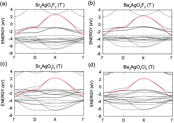
Figure 12: (Color online) Electronic band structure of one-band Hamiltonian in the LDA originating from the Ag $d_{x^{2}-y^{2}}$ anti-bonding Wannier orbital. The zero energy corresponds to the Fermi level. For comparison, the band structures in the LDA is also given (black dotted line).

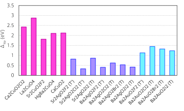
Figure 13: (Color online) Difference of the onsite potential between the $x^{2}-y^{2}$ and the $2p$ orbitals.

Figure 14: (Color online) Electronic band structure of three-band $dpp$ Hamiltonian in the LDA originating from the Ag $d_{x^{2}-y^{2}}$ and the O $2p$ Wannier orbitals. The zero energy corresponds to the Fermi level. For comparison, the band structures in the LDA is also given (black dotted line).

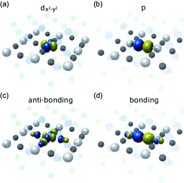
Figure 15: (Color online) Isosurface of the maximally localized Wannier function for $\pm 0.07$ a.u for (a) the Ag $d_{x^{2}-y^{2}}$ orbital, (b) the O $p$ orbital, and (c) anti-bonding and (d) bonding orbitals consisting of the Ag $x^{2}-y^{2}$ and O $p$ orbital of Sr₂AgO₂F₂ (T’).

Figure 12 shows the band dispersion of one-band Hamiltonians constructed from the Wannier orbital for several Ag-based oxides at the LDA level. We show the DFT/LDA band structure as a comparison.

Next, we consider the three-band Hamiltonian. Figure 14 shows the fitting of the band dispersion in the three-band Hamiltonian for the Ag $x^{2}-y^{2}$ and the O $2p$ orbitals of some Ag-based oxides. We also show the corresponding Wannier functions of the Ag $x^{2}-y^{2}$, the O $2p$ orbitals, and the antibonding and bonding orbitals in Fig. 15. There are three important parameters in the three-band Hamiltonian that characterize $U/t$ of the one-band Hamiltonian: hopping between the $x^{2}-y^{2}$ and $2p$ orbitals $t_{dp}$, the on-site potential difference between the $x^{2}-y^{2}$ and $2p$ orbitals $\Delta_{dp}$, and dielectric constant for the $x^{2}-y^{2}$ and $2p$ orbitals $U/v$, where $v$ is the bare Coulomb interaction. Figure 13 shows the comparison of $\Delta_{dp}$ for the copper, silver, and gold oxides. We find that the Ag compounds are strongly covalent systems because the energies of the $x^{2}-y^{2}$ and $2p$ orbitals are very close, while the Au compounds have intermediate values of $\Delta_{dp}$. We summarize other parameters including $\Delta_{dp}$ and $U/v$ in Tables 9, 10, and  11.

The three parameters, $t_{dp}$, $\Delta_{dp}$ and $U/v$ show a relation with the lattice constant $a$. Figure 16(a) shows hopping $t_{dp}$ versus $a$ for Ag oxides. Regardless of the type of the structure, the hopping $t_{dp}$ decreases monotonically with increasing lattice constant $a$ as is naturally expected. Figure 16(b) shows the energy difference $\Delta_{dp}$. Due to ionic stability, Ag is mainly surrounded by anions and O is mainly surrounded by cations. As the lattice constants become smaller, the energy difference between the $x^{2}-y^{2}$ and $2p$ orbitals also becomes larger because they are more susceptible to the electric field from them. Although Ba₂AgO₂I₂ is out of trend, $U/v$ also have relations with the lattice constant $a$ (Fig. 16(c)). This is because elements with smaller ionic radii are more stable in their closed-shell states, and their bands tend to appear farther away from the Fermi level, thus producing less screening effects.

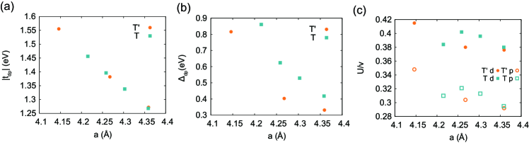
Figure 16: (Color online) Nearest neighbor hopping $t_{dp}$ and on-site potential difference between the Ag $x^{2}-y^{2}$ and the O $p$ orbitals, $\Delta_{dp}$ and $|U/v|$ for the Ag $x^{2}-y^{2}$ and the O $p$ orbitals plotted against the lattice constant $a$.

Table 9: On-site potentials and effective interactions for three-band $dpp$ Hamiltonian of Cu-based compounds (in eV). The one-body part is obtained from the fitting of the LDA band structure, while the effective interaction is the result of the cRPA from the LDA bands. $v$, $U$, and $J$ represent the bare Coulomb, the static values of the effective Coulomb, and exchange interactions, respectively (at $\omega=0$).

Ca2CuO2Cl2		$t(0,0,0)$			$v(0,0,0)$			$U(0,0,0)$			$J(0,0,0)$
	$x^{2}-y^{2}$	$p_{1}$	$p_{2}$	$x^{2}-y^{2}$	$p_{1}$	$p_{2}$	$x^{2}-y^{2}$	$p_{1}$	$p_{2}$	$x^{2}-y^{2}$	$p_{1}$	$p_{2}$
$x^{2}-y^{2}$	-1.877	-1.279	1.279	28.824	8.099	8.099	9.740	2.613	2.613		0.048	0.048
$p_{1}$	-1.279	-4.301	-0.640	8.099	17.524	5.416	2.613	6.194	1.727	0.048		0.021
$p_{2}$	1.279	-0.640	-4.301	8.099	5.416	17.524	2.613	1.727	6.194	0.048	0.021
La2CuO4		$t(0,0,0)$			$v(0,0,0)$			$U(0,0,0)$			$J(0,0,0)$
	$x^{2}-y^{2}$	$p_{1}$	$p_{2}$	$x^{2}-y^{2}$	$p_{1}$	$p_{2}$	$x^{2}-y^{2}$	$p_{1}$	$p_{2}$	$x^{2}-y^{2}$	$p_{1}$	$p_{2}$
$x^{2}-y^{2}$	-2.052	-1.403	1.403	28.782	8.247	8.246	8.717	1.908	1.908		0.049	0.049
$p_{1}$	-1.403	-4.926	-0.666	8.247	17.773	5.501	1.908	5.330	1.124	0.049		0.019
$p_{2}$	1.403	-0.666	-4.926	8.246	5.501	17.773	1.908	1.124	5.330	0.049	0.019
Sr2CuO2F2		$t(0,0,0)$			$v(0,0,0)$			$U(0,0,0)$			$J(0,0,0)$
	$x^{2}-y^{2}$	$p_{1}$	$p_{2}$	$x^{2}-y^{2}$	$p_{1}$	$p_{2}$	$x^{2}-y^{2}$	$p_{1}$	$p_{2}$	$x^{2}-y^{2}$	$p_{1}$	$p_{2}$
$x^{2}-y^{2}$	-1.798	-1.155	1.155	28.649	7.917	7.917	9.067	2.438	2.438		0.049	0.049
$p_{1}$	-1.155	-3.609	-0.633	7.917	16.918	5.278	2.438	5.774	1.672	0.049		0.023
$p_{2}$	1.155	-0.633	-3.609	7.917	5.278	16.918	2.438	1.672	5.774	0.049	0.023
HgBa2CuO4		$t(0,0,0)$			$v(0,0,0)$			$U(0,0,0)$			$J(0,0,0)$
	$x^{2}-y^{2}$	$p_{1}$	$p_{2}$	$x^{2}-y^{2}$	$p_{1}$	$p_{2}$	$x^{2}-y^{2}$	$p_{1}$	$p_{2}$	$x^{2}-y^{2}$	$p_{1}$	$p_{2}$
$x^{2}-y^{2}$	-2.311	-1.261	1.261	28.820	8.010	8.010	8.539	1.844	1.844		0.048	0.048
$p_{1}$	-1.261	-4.416	-0.634	8.010	17.114	5.319	1.844	5.170	1.098	0.048		0.020
$p_{2}$	1.261	-0.634	-4.416	8.010	5.319	17.114	1.844	1.098	5.170	0.048	0.020
CaCuO2		$t(0,0,0)$			$v(0,0,0)$			$U(0,0,0)$			$J(0,0,0)$
	$x^{2}-y^{2}$	$p_{1}$	$p_{2}$	$x^{2}-y^{2}$	$p_{1}$	$p_{2}$	$x^{2}-y^{2}$	$p_{1}$	$p_{2}$	$x^{2}-y^{2}$	$p_{1}$	$p_{2}$
$x^{2}-y^{2}$	-1.914	-1.295	1.295	28.993	8.120	8.120	8.906	2.086	2.086		0.047	0.047
$p_{1}$	-1.295	-4.036	-0.633	8.120	17.844	5.410	2.086	5.883	1.257	0.047		0.018
$p_{2}$	1.295	-0.633	-4.036	8.120	5.410	17.844	2.086	1.257	5.883	0.047	0.018

Table 10: On-site potentials and effective interactions for three-band $dpp$ Hamiltonian of Ag-based compounds (in eV). The one-body part is obtained from the fitting of the LDA band structure, while the effective interaction is the result of the cRPA from the LDA bands. $v$, $U$, and $J$ represent the bare Coulomb, the static values of the effective Coulomb, and exchange interactions, respectively (at $\omega=0$).

Sr2AgO2F2 (T’)		$t(0,0,0)$			$v(0,0,0)$			$U(0,0,0)$			$J(0,0,0)$
	$x^{2}-y^{2}$	$p_{1}$	$p_{2}$	$x^{2}-y^{2}$	$p_{1}$	$p_{2}$	$x^{2}-y^{2}$	$p_{1}$	$p_{2}$	$x^{2}-y^{2}$	$p_{1}$	$p_{2}$
$x^{2}-y^{2}$	-2.900	-1.555	1.554	19.455	7.519	7.519	8.083	2.645	2.645		0.064	0.064
$p_{1}$	-1.555	-3.716	-0.584	7.519	17.012	5.030	2.645	5.913	1.725	0.064		0.020
$p_{2}$	1.554	-0.584	-3.716	7.519	5.030	17.012	2.645	1.725	5.913	0.064	0.020
Sr2AgO2Cl2 (T’)		$t(0,0,0)$			$v(0,0,0)$			$U(0,0,0)$			$J(0,0,0)$
	$x^{2}-y^{2}$	$p_{1}$	$p_{2}$	$x^{2}-y^{2}$	$p_{1}$	$p_{2}$	$x^{2}-y^{2}$	$p_{1}$	$p_{2}$	$x^{2}-y^{2}$	$p_{1}$	$p_{2}$
$x^{2}-y^{2}$	-2.641	-1.272	1.272	19.514	7.164	7.164	7.335	1.818	1.818		0.055	0.055
$p_{1}$	-1.272	-2.972	-0.505	7.164	16.845	4.793	1.818	4.927	1.035	0.055		0.017
$p_{2}$	1.272	-0.505	-2.972	7.164	4.793	16.845	1.818	1.035	4.927	0.055	0.017
Sr2AgO2I2 (T)		$t(0,0,0)$			$v(0,0,0)$			$U(0,0,0)$			$J(0,0,0)$
	$x^{2}-y^{2}$	$p_{1}$	$p_{2}$	$x^{2}-y^{2}$	$p_{1}$	$p_{2}$	$x^{2}-y^{2}$	$p_{1}$	$p_{2}$	$x^{2}-y^{2}$	$p_{1}$	$p_{2}$
$x^{2}-y^{2}$	-2.888	-1.456	1.456	19.483	7.387	7.387	7.479	2.042	2.042		0.060	0.060
$p_{1}$	-1.456	-3.749	-0.548	7.387	16.935	4.947	2.042	5.244	1.251	0.060		0.018
$p_{2}$	1.456	-0.548	-3.749	7.387	4.947	16.935	2.042	1.251	5.244	0.060	0.018
Ba2AgO2F2 (T’)		$t(0,0,0)$			$v(0,0,0)$			$U(0,0,0)$			$J(0,0,0)$
	$x^{2}-y^{2}$	$p_{1}$	$p_{2}$	$x^{2}-y^{2}$	$p_{1}$	$p_{2}$	$x^{2}-y^{2}$	$p_{1}$	$p_{2}$	$x^{2}-y^{2}$	$p_{1}$	$p_{2}$
$x^{2}-y^{2}$	-2.785	-1.382	1.382	19.464	7.299	7.299	7.400	2.044	2.044		0.061	0.061
$p_{1}$	-1.382	-3.188	-0.551	7.299	16.646	4.880	2.044	5.066	1.271	0.061		0.019
$p_{2}$	1.382	-0.551	-3.188	7.299	4.880	16.646	2.044	1.271	5.066	0.061	0.019
Ba2AgO2Cl2 (T)		$t(0,0,0)$			$v(0,0,0)$			$U(0,0,0)$			$J(0,0,0)$
	$x^{2}-y^{2}$	$p_{1}$	$p_{2}$	$x^{2}-y^{2}$	$p_{1}$	$p_{2}$	$x^{2}-y^{2}$	$p_{1}$	$p_{2}$	$x^{2}-y^{2}$	$p_{1}$	$p_{2}$
$x^{2}-y^{2}$	-2.762	-1.396	1.396	19.455	7.307	7.307	7.815	2.247	2.247		0.059	0.059
$p_{1}$	-1.396	-3.386	-0.535	7.307	16.794	4.892	2.247	5.395	1.405	0.059		0.018
$p_{2}$	1.396	-0.535	-3.386	7.307	4.892	16.794	2.247	1.405	5.395	0.059	0.018
Ba2AgO2Br2 (T)		$t(0,0,0)$			$v(0,0,0)$			$U(0,0,0)$			$J(0,0,0)$
	$x^{2}-y^{2}$	$p_{1}$	$p_{2}$	$x^{2}-y^{2}$	$p_{1}$	$p_{2}$	$x^{2}-y^{2}$	$p_{1}$	$p_{2}$	$x^{2}-y^{2}$	$p_{1}$	$p_{2}$
$x^{2}-y^{2}$	-2.727	-1.338	1.338	19.464	7.226	7.226	7.703	2.112	2.112		0.058	0.058
$p_{1}$	-1.338	-3.256	-0.524	7.226	16.644	4.83	2.112	5.202	1.302	0.058		0.018
$p_{2}$	1.338	-0.524	-3.256	7.226	4.838	16.644	2.112	1.302	5.202	0.058	0.018
Ba2AgO2I2 (T)		$t(0,0,0)$			$v(0,0,0)$			$U(0,0,0)$			$J(0,0,0)$
	$x^{2}-y^{2}$	$p_{1}$	$p_{2}$	$x^{2}-y^{2}$	$p_{1}$	$p_{2}$	$x^{2}-y^{2}$	$p_{1}$	$p_{2}$	$x^{2}-y^{2}$	$p_{1}$	$p_{2}$
$x^{2}-y^{2}$	-2.737	-1.268	1.268	19.450	7.131	7.131	7.387	1.866	1.866		0.057	0.057
$p_{1}$	-1.268	-3.155	-0.512	7.131	16.475	4.776	1.866	4.862	1.124	0.057		0.018
$p_{2}$	1.268	-0.512	-3.155	7.131	4.776	16.475	1.866	1.124	4.862	0.057	0.018

Table 11: On-site potentials and effective interactions for three-band $dpp$ Hamiltonian of Au-based compounds (in eV). The one-body part is obtained from the fitting of the LDA band structure, while the effective interaction is the result of the cRPA from the LDA bands. $v$, $U$, and $J$ represent the bare Coulomb, the static values of the effective Coulomb, and exchange interactions, respectively (at $\omega=0$).

Ba2AuO2F2 (T’)		$t(0,0,0)$			$v(0,0,0)$			$U(0,0,0)$			$J(0,0,0)$
	$x^{2}-y^{2}$	$p_{1}$	$p_{2}$	$x^{2}-y^{2}$	$p_{1}$	$p_{2}$	$x^{2}-y^{2}$	$p_{1}$	$p_{2}$	$x^{2}-y^{2}$	$p_{1}$	$p_{2}$
$x^{2}-y^{2}$	-2.811	-1.591	1.591	16.628	7.282	7.282	6.414	1.968	1.968		0.092	0.092
$p_{1}$	-1.591	-3.940	-0.701	7.282	15.835	4.899	1.968	4.587	1.230	0.092		0.027
$p_{2}$	1.591	-0.701	-3.940	7.282	4.899	15.835	1.968	1.230	4.587	0.092	0.027
Ba2AuO2Cl2 (T)		$t(0,0,0)$			$v(0,0,0)$			$U(0,0,0)$			$J(0,0,0)$
	$x^{2}-y^{2}$	$p_{1}$	$p_{2}$	$x^{2}-y^{2}$	$p_{1}$	$p_{2}$	$x^{2}-y^{2}$	$p_{1}$	$p_{2}$	$x^{2}-y^{2}$	$p_{1}$	$p_{2}$
$x^{2}-y^{2}$	-2.772	-1.626	1.626	16.537	7.293	7.293	6.292	1.962	1.962		0.092	0.092
$p_{1}$	-1.626	-4.223	-0.696	7.293	15.823	4.922	1.962	4.635	1.228	0.092		0.027
$p_{2}$	1.626	-0.696	-4.223	7.293	4.922	15.823	1.962	1.228	4.635	0.092	0.027
Ba2AuO2Br2 (T)		$t(0,0,0)$			$v(0,0,0)$			$U(0,0,0)$			$J(0,0,0)$
	$x^{2}-y^{2}$	$p_{1}$	$p_{2}$	$x^{2}-y^{2}$	$p_{1}$	$p_{2}$	$x^{2}-y^{2}$	$p_{1}$	$p_{2}$	$x^{2}-y^{2}$	$p_{1}$	$p_{2}$
$x^{2}-y^{2}$	-2.740	-1.564	1.564	16.553	7.227	7.227	6.160	1.799	1.799		0.091	0.091
$p_{1}$	-1.564	-4.064	-0.684	7.227	15.693	4.876	1.799	4.409	1.098	0.091		0.027
$p_{2}$	1.564	-0.684	-4.064	7.227	4.876	15.693	1.799	1.098	4.409	0.091	0.027
Ba2AuO2I2 (T)		$t(0,0,0)$			$v(0,0,0)$			$U(0,0,0)$			$J(0,0,0)$
	$x^{2}-y^{2}$	$p_{1}$	$p_{2}$	$x^{2}-y^{2}$	$p_{1}$	$p_{2}$	$x^{2}-y^{2}$	$p_{1}$	$p_{2}$	$x^{2}-y^{2}$	$p_{1}$	$p_{2}$
$x^{2}-y^{2}$	-2.722	-1.483	1.483	16.557	7.137	7.137	6.037	1.688	1.688		0.089	0.089
$p_{1}$	-1.483	-3.955	-0.667	7.137	15.531	4.815	1.688	4.234	1.018	0.089		0.027
$p_{2}$	1.483	-0.667	-3.955	7.137	4.815	15.531	1.688	1.018	4.234	0.089	0.027

Appendix D Band structure and effective Hamiltonians on the GWA level

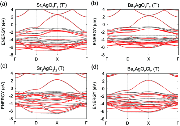
Figure 17: (Color online) Electronic band structures of Ag-based compounds obtained by the GWA illustrated as red curves. Self-energy is calculated only for the LDA 17 bands originating from the Ag $4d$ and O $2p$ orbitals near the Fermi level indicated by gray in black and white plot bands. The zero energy corresponds to the Fermi level.

Figure 17 shows the band structures in the GWA. The band widths of the antibonding orbitals are approximately unchanged from the LDA. This is because silver atoms are weakly correlated compared to the $3d$ elements such as copper atoms, and therefore the effect of self-energy correction of the GWA is small. Halogen, on the other hand, has a small bandwidth and is shifted away from the Fermi level in the GWA. Such a change has a significant effect on the screening effects. Band structures for the one-band and three-band $dpp$ Hamiltonians on the GW level are also shown in Fig. 18 and 19, respectively.

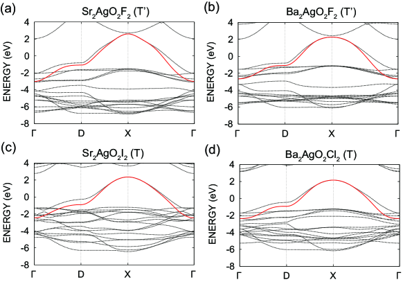
Figure 18: (Color online) Electronic band structure of one-band Hamiltonian in the GWA originating from the Ag $d_{x^{2}-y^{2}}$ anti-bonding Wannier orbital. The zero energy corresponds to the Fermi level. For comparison, the band structures in the GWA is also given (black dotted line).

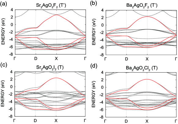
Figure 19: (Color online) Electronic band structure of three-band $dpp$ Hamiltonian in the GWA originating from the Ag $d_{x^{2}-y^{2}}$ and the O $2p$ Wannier orbitals. The zero energy corresponds to the Fermi level. For comparison, the band structures in the GWA is also given (black dotted line).

D.1 Downfolding

Here, we derive low-energy effective Hamiltonians from the GW band structure.

D.1.1 Derivation of one-band Hamiltonian

First, as in the LDA calculations, we summarize the parameters of the one-band Hamiltonian, the hopping calculated from the maximally localized Wannier orbitals constructed from the GW band and the effective interaction obtained by the cRPA, in Table 12. The $U/t$ values are larger than that in the LDA due to the self-energy effect, with the largest value being about 6.5.

D.1.2 Derivation of three-band $dpp$ Hamiltonian

We also summarize the three-band Hamiltonian in Table 13. The difference in the on-site potential between the Ag $x^{2}-y^{2}$ and O $2p$ orbitals $\Delta_{dp}$ is almost unchanged from that in the LDA. This is because, unlike copper oxides, Ag does not have a significantly larger Coulomb interaction than O. On the other hand, $U/v$ increases significantly because of the reduction of the screening effects owing to poor polarization by the orbitals with small bandwidth such as halogens.

Table 12: On-site potentials and effective interactions for one-band Hamiltonian of Ag-based compounds (in eV). The one-body part is obtained from the fitting of the GW band structure, while the effective interaction is the result of the cRPA from the GW bands. $v$, $U$, and $V$ represent the bare Coulomb, the static values of the effective on-site Coulomb, and the effective off-site Coulomb, respectively (at $\omega=0$). $U/v$ is the ratio of the on-site bare and screened Coulomb interactions, and $U/t$ is the ratio of the nearest neighbor hopping and the screened Coulomb interaction.

	$t(1,0,0)$	$t(1,1,0)$	$t(2,0,0)$	$v(0,0,0)$	$U(0,0,0)$	$v(1,0,0)$	$V(1,0,0)$	$v(1,1,0)$	$V(1,1,0)$	$U/v$	$U/t$
Sr2AgO2F2 (T’)	-0.682	0.088	-0.094	11.964	4.401	3.982	1.464	2.603	0.966	0.368	6.45
Ba2AgO2F2 (T’)	-0.661	0.100	-0.091	11.485	4.010	3.894	1.282	2.533	0.811	0.349	6.07
Sr2AgO2I2 (T)	-0.595	0.111	-0.094	11.063	3.337	3.907	0.938	2.564	0.535	0.302	5.61
Ba2AgO2Cl2 (T)	-0.600	0.079	-0.081	11.434	3.728	3.881	1.115	2.536	0.694	0.326	6.21

Table 13: On-site potentials and effective interactions for three-band Hamiltonian of Ag-based compounds (in eV). The one-body part is obtained from the fitting of the GW band structure, while the effective interaction is the result of the cRPA form the GW bands. $v$, $U$, and $J$ represent the bare Coulomb, the static values of the effective Coulomb, and exchange interactions, respectively (at $\omega=0$).

Sr2AgO2F2 (T’)		$t(0,0,0)$			$v(0,0,0)$			$U(0,0,0)$			$J(0,0,0)$
	$x^{2}-y^{2}$	$p_{1}$	$p_{2}$	$x^{2}-y^{2}$	$p_{1}$	$p_{2}$	$x^{2}-y^{2}$	$p_{1}$	$p_{2}$	$x^{2}-y^{2}$	$p_{1}$	$p_{2}$
$x^{2}-y^{2}$	-2.992	-1.534	1.534	19.455	7.519	7.519	8.493	2.865	2.865		0.064	0.064
$p_{1}$	-1.534	-3.783	-0.607	7.519	17.012	5.030	2.865	6.213	1.891	0.064		0.020
$p_{2}$	1.534	-0.607	-3.783	7.519	5.030	17.012	2.865	1.891	6.213	0.064	0.020
Ba2AgO2F2 (T’)		$t(0,0,0)$			$v(0,0,0)$			$U(0,0,0)$			$J(0,0,0)$
	$x^{2}-y^{2}$	$p_{1}$	$p_{2}$	$x^{2}-y^{2}$	$p_{1}$	$p_{2}$	$x^{2}-y^{2}$	$p_{1}$	$p_{2}$	$x^{2}-y^{2}$	$p_{1}$	$p_{2}$
$x^{2}-y^{2}$	-2.846	-1.361	1.361	19.464	7.299	7.299	8.399	2.652	2.652		0.061	0.061
$p_{1}$	-1.361	-3.186	-0.578	7.299	16.646	4.880	2.652	5.834	1.716	0.061		0.019
$p_{2}$	1.361	-0.578	-3.186	7.299	4.880	16.646	2.652	1.716	5.834	0.061	0.019
Sr2AgO2I2 (T)		$t(0,0,0)$			$v(0,0,0)$			$U(0,0,0)$			$J(0,0,0)$
	$x^{2}-y^{2}$	$p_{1}$	$p_{2}$	$x^{2}-y^{2}$	$p_{1}$	$p_{2}$	$x^{2}-y^{2}$	$p_{1}$	$p_{2}$	$x^{2}-y^{2}$	$p_{1}$	$p_{2}$
$x^{2}-y^{2}$	-2.721	-1.413	1.413	19.483	7.387	7.387	7.672	2.144	2.144		0.060	0.060
$p_{1}$	-1.413	-3.568	-0.560	7.387	16.935	4.947	2.144	5.370	1.320	0.060		0.018
$p_{2}$	1.413	-0.560	-3.568	7.387	4.947	16.935	2.144	1.320	5.370	0.060	0.028
Ba2AgO2Cl2 (T)		$t(0,0,0)$			$v(0,0,0)$			$U(0,0,0)$			$J(0,0,0)$
	$x^{2}-y^{2}$	$p_{1}$	$p_{2}$	$x^{2}-y^{2}$	$p_{1}$	$p_{2}$	$x^{2}-y^{2}$	$p_{1}$	$p_{2}$	$x^{2}-y^{2}$	$p_{1}$	$p_{2}$
$x^{2}-y^{2}$	-2.712	-1.351	1.351	19.455	7.307	7.307	7.971	2.321	2.321		0.059	0.059
$p_{1}$	-1.351	-3.301	-0.544	7.307	16.794	4.892	2.321	5.501	1.457	0.059		0.018
$p_{2}$	1.351	-0.544	-3.301	7.307	4.892	16.794	2.321	1.457	5.501	0.059	0.018

Appendix E Three-band $dpp$ effective Hamiltonians at the GW level for four Ag-based compounds

Table 14 shows the parameters of the three-band Hamiltonian calculated at the cGW-SIC level for the four Ag compounds. The two-body terms are the same as the GW level (see Table 13 shown in Appendix D). We illustrate the corresponding band structure of the one-body term in Fig. 20. The band width is close to that of the LDA level. This is because the double counting of low-energy degrees of freedom to be subtracted and the renormalization arising from the frequency dependence of the interaction more or less cancel out, as is also seen in SrVO₃ and others hirayama17 . However, the energy difference between the $x^{2}-y^{2}$ and O $2p$ orbitals $\Delta_{dp}$ and hopping substantially change from those of the fitting, which have a significant impact on the correlation of the system and the stability of the superconductivity.

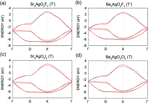
Figure 20: (Color online) Electronic band structure of three-band $dpp$ Hamiltonian at the cGW-SIC level originating from the Ag $d_{x^{2}-y^{2}}$ and the O $2p$ Wannier orbitals for the four Ag compounds. The zero energy corresponds to the Fermi level. For comparison, the fitting band structure for the GWA is also given (black dotted line).

Table 14: On-site potentials and effective interactions for three-band $dpp$ Hamiltonian of Ag-based compounds (in eV). The transfer integral is the result of the cGW-SIC from the GW bands, while the effective interaction is the result of the cRPA from the GW bands. $v$, $U$, and $J$ represent the bare Coulomb, the static values of the effective Coulomb, and exchange interactions, respectively (at $\omega=0$).

Sr2AgO2F2 (T’)		$t(0,0,0)$			$v(0,0,0)$			$U(0,0,0)$			$J(0,0,0)$
	$x^{2}-y^{2}$	$p_{1}$	$p_{2}$	$x^{2}-y^{2}$	$p_{1}$	$p_{2}$	$x^{2}-y^{2}$	$p_{1}$	$p_{2}$	$x^{2}-y^{2}$	$p_{1}$	$p_{2}$
$x^{2}-y^{2}$	-3.091	-1.562	1.562	19.455	7.519	7.519	8.493	2.865	2.865		0.064	0.064
$p_{1}$	-1.562	-3.702	-0.688	7.519	17.012	5.030	2.865	6.213	1.891	0.064		0.020
$p_{2}$	1.562	-0.688	-3.702	7.519	5.030	17.012	2.865	1.891	6.213	0.064	0.020
Ba2AgO2F2 (T’)		$t(0,0,0)$			$v(0,0,0)$			$U(0,0,0)$			$J(0,0,0)$
	$x^{2}-y^{2}$	$p_{1}$	$p_{2}$	$x^{2}-y^{2}$	$p_{1}$	$p_{2}$	$x^{2}-y^{2}$	$p_{1}$	$p_{2}$	$x^{2}-y^{2}$	$p_{1}$	$p_{2}$
$x^{2}-y^{2}$	-3.034	-1.388	1.388	19.464	7.299	7.299	8.399	2.652	2.652		0.061	0.061
$p_{1}$	-1.388	-3.039	-0.648	7.299	16.646	4.880	2.652	5.834	1.716	0.061		0.019
$p_{2}$	1.388	-0.648	-3.039	7.299	4.880	16.646	2.652	1.716	5.834	0.061	0.019
Sr2AgO2I2 (T)		$t(0,0,0)$			$v(0,0,0)$			$U(0,0,0)$			$J(0,0,0)$
	$x^{2}-y^{2}$	$p_{1}$	$p_{2}$	$x^{2}-y^{2}$	$p_{1}$	$p_{2}$	$x^{2}-y^{2}$	$p_{1}$	$p_{2}$	$x^{2}-y^{2}$	$p_{1}$	$p_{2}$
$x^{2}-y^{2}$	-2.724	-1.465	1.465	19.483	7.387	7.387	7.672	2.144	2.144		0.060	0.060
$p_{1}$	-1.465	-3.409	-0.637	7.387	16.935	4.947	2.144	5.370	1.320	0.060		0.018
$p_{2}$	1.465	-0.637	-3.409	7.387	4.947	16.935	2.144	1.320	5.370	0.060	0.028
Ba2AgO2Cl2 (T)		$t(0,0,0)$			$v(0,0,0)$			$U(0,0,0)$			$J(0,0,0)$
	$x^{2}-y^{2}$	$p_{1}$	$p_{2}$	$x^{2}-y^{2}$	$p_{1}$	$p_{2}$	$x^{2}-y^{2}$	$p_{1}$	$p_{2}$	$x^{2}-y^{2}$	$p_{1}$	$p_{2}$
$x^{2}-y^{2}$	-2.827	-1.400	1.400	19.455	7.307	7.307	7.971	2.321	2.321		0.059	0.059
$p_{1}$	-1.400	-3.162	-0.619	7.307	16.794	4.892	2.321	5.501	1.457	0.059		0.018
$p_{2}$	1.400	-0.619	-3.162	7.307	4.892	16.794	2.321	1.457	5.501	0.059	0.018

Appendix F Full parameters of one-band Hamiltonian for Sr₂AgO₂F₂

We summarize the full parameters of one-band Hamiltonian for Sr₂AgO₂F₂ in Table 15.

Table 15: Full parameters of transfer integral and effective interaction (in eV) in one-band Hamiltonian for Sr₂AgO₂F₂ used for the present calculation. The notations are the same as Table 6. A part of parameters is given in Table 6.

$t(1,0,0)$	$t(1,1,0)$	$t(2,0,0)$	$t(2,1,0)$	$t(2,2,0)$	$t(3,0,0)$	$t(3,1,0)$	$t(3,2,0)$	$t(3,3,0)$
-0.6577	0.0920	-0.1014	0.0171	-0.0078	-0.0292	0.0180	-0.0046	-0.0038
$v(0,0,0)$	$U(0,0,0)$	$V(1,0,0)$	$V(1,1,0)$	$V(2,0,0)$	$V(2,1,0)$	$V(2,2,0)$	$V(3,0,0)$	$V(3,1,0)$	$V(3,2,0)$	$V(3,3,0)$
11.964	4.401	1.464	0.966	0.771	0.683	0.583	0.640	0.600	0.544	0.520

Appendix G Ca-doping

Here, we show the effect of Ca-doping to alkaline earth cation. Ca₂AgO₂F₂ itself is unstable, but the system with carrier doping or partial substitution for Ca might be stable. Figure 21 shows the nearest neighbor hopping and the on-site potential of Ca₂AgO₂F₂ in the LDA. Both $t$ and $U$ become larger than those of Sr and Ba systems, while keeping the magnitude of $U/t$ approximately the same. We summarize the parameter for Ca₂AgO₂F₂ in Tables. 16 and  17.

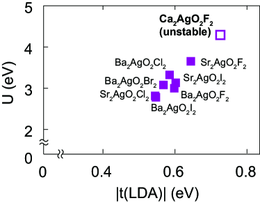
Figure 21: (Color online) Nearest neighbor hopping and on-site interaction in the Ag-based superconductors including unstable Ca₂AgO₂F₂ in the LDA.

Table 16: Transfer integral and effective interaction in one-band Hamiltonian for Ca₂AgO₂F₂ (T’) (in eV). The one-body part is obtained from the fitting of the LDA band structure, while the effective interaction is the result of the cRPA. $v$, $U$, and $V$ represent the bare Coulomb, the static values of the effective on-site Coulomb, and the effective off-site Coulomb, respectively (at $\omega=0$). $U/v$ is the ratio of the on-site bare and screened Coulomb interactions, and $U/t$ is the ratio of the nearest neighbor hopping and the screened Coulomb interaction.

LDA	$t(1,0,0)$	$t(1,1,0)$	$t(2,0,0)$	$v(0,0,0)$	$U(0,0,0)$	$v(1,0,0)$	$V(1,0,0)$	$v(1,1,0)$	$V(1,1,0)$	$v(2,0,0)$	$V(2,0,0)$	$U/v$	$|U/t|$
$x^{2}-y^{2}$	-0.726	0.109	-0.098	12.059	4.291	4.068	1.410	2.671	0.915	2.011	0.717	0.356	5.91

Table 17: On-site potentials and effective interactions for three-band $dpp$ Hamiltonian of Ca₂AgO₂F₂ (T’) (in eV). The one-body part is obtained from the fitting of the LDA and GW band structures and the cGW-SIC, while the effective interaction is the result of the cRPA. $v$, $U$, and $J$ represent the bare Coulomb, the static values of the effective Coulomb, and exchange interactions, respectively (at $\omega=0$).

LDA		$t(0,0,0)$			$v(0,0,0)$			$U(0,0,0)$			$J(0,0,0)$
	$x^{2}-y^{2}$	$p_{1}$	$p_{2}$	$x^{2}-y^{2}$	$p_{1}$	$p_{2}$	$x^{2}-y^{2}$	$p_{1}$	$p_{2}$	$x^{2}-y^{2}$	$p_{1}$	$p_{2}$
$x^{2}-y^{2}$	-3.043	-1.715	1.715	19.392	7.707	7.707	8.167	2.837	2.837		0.067	0.067
$p_{1}$	-1.715	-4.214	-0.615	7.707	17.012	5.030	2.837	6.218	1.891	0.067		0.020
$p_{2}$	1.715	-0.615	-4.214	7.707	5.030	17.012	2.837	1.891	6.218	0.067	0.020
GW		$t(0,0,0)$			$v(0,0,0)$			$U(0,0,0)$			$J(0,0,0)$
	$x^{2}-y^{2}$	$p_{1}$	$p_{2}$	$x^{2}-y^{2}$	$p_{1}$	$p_{2}$	$x^{2}-y^{2}$	$p_{1}$	$p_{2}$	$x^{2}-y^{2}$	$p_{1}$	$p_{2}$
$x^{2}-y^{2}$	-3.101	-1.695	1.695	19.392	7.704	7.704	8.330	2.854	2.854		0.067	0.067
$p_{1}$	-1.695	-4.287	-0.639	7.704	17.300	5.163	2.854	6.252	1.882	0.067		0.020
$p_{2}$	1.695	-0.639	-4.287	7.704	5.163	17.300	2.854	1.882	6.252	0.067	0.020
cGW-SIC		$t(0,0,0)$			$v(0,0,0)$			$U(0,0,0)$			$J(0,0,0)$
	$x^{2}-y^{2}$	$p_{1}$	$p_{2}$	$x^{2}-y^{2}$	$p_{1}$	$p_{2}$	$x^{2}-y^{2}$	$p_{1}$	$p_{2}$	$x^{2}-y^{2}$	$p_{1}$	$p_{2}$
$x^{2}-y^{2}$	-3.045	-1.648	1.648	19.392	7.704	7.704	8.330	2.854	2.854		0.067	0.067
$p_{1}$	-1.648	-4.047	-0.669	7.704	17.300	5.163	2.854	6.252	1.882	0.067		0.020
$p_{2}$	1.648	-0.669	-4.047	7.704	5.163	17.300	2.854	1.882	6.252	0.067	0.020
occ.(GWA)	$x^{2}-y^{2}$	$p_{1}$	$p_{2}$
	1.518	1.741	1.741

References

- (1) Bednortz and A Müller, Z. Phys. 87, 195144 (1986).
- (2) M. Hirayama, Y. Yamaji, T. Misawa, and M. Imada, Phys. Rev. B 98, 134501 (2018).
- (3) M. Hirayama, T. Misawa, T. Ohgoe, Y. Yamaji, and M. Imada, Phys. Rev. B 99, 245155 (2019).
- (4) T. Ohgoe, M. Hirayama, T. Misawa, K. Ido, Y. Yamaji and M. Imada, Phys. Rev. B 101, 045124 (2020).
- (5) J. M. Tranquada, J. D. Axe, N. Ichikawa, A. R. Moodenbaugh, Y. Nakamura, and S. Uchida, Phys. Rev. Lett. 78, 338 (1997).
- (6) S. Pan, J. P. O’Neal, R. L. Badzey, et al., Nature 413, 282 (2001).
- (7) M. Imada, A. Fujimori and Y. Tokura, Rev. Mod Phys. 70, 1039 (1998).
- (8) M. Imada and T. Miyake, J. Phys. Soc. Jpn. 79, 112001 (2010).
- (9) M. Hirayama, T. Miyake, and M. Imada, Phys. Rev. B 87, 195144 (2013).
- (10) F. Aryasetiawan, M. Imada, A. Georges, G. Kotliar, S. Biermann, and A. I. Lichtenstein, Phys. Rev. B 70, 195104 (2004).
- (11) M. Hirayama, T. Miyake, M. Imada and S. Biermann, Phys. Rev. B. 96, 075102 (2017).
- (12) T. Misawa and M. Imada, Phys. Rev. B 90, 115137 (2014).
- (13) T. Misawa, Y. Nomura, S. Biermann and M. Imada, Sci. Adv. 2, e1600664 (2016).
- (14) M. Imada and T. J. Suzuki, J. Phys. Soc. Jpn. 88, 024701 (2019).
- (15) M. Imada, J. Phys. Soc. Jpn. 90, 111009 (2021).
- (16) F. Nilsson, K. Karlsson, and F. Aryasetiawan, Phys. Rev. B 99, 075135 (2019).
- (17) J.-B. Morée M. Hirayama, M. T. Schmid, Y. Yamaji, and M. Imada, arXiv:2206.01510.
- (18) H. Kageyama, K. Hayashi, K. Maeda, J. P. Attfield, Z. Hiroi, J. M. Rondinelli, and K. R. Poeppelmeier, Nat. Commun. 9, 772 (2018).
- (19) J. L. Kissick, C. Greaves, P. P. Edwards, V. M. Cherkashenko, E. Z. Kurmaev, S. Bartkowski, and M. Neumann, Phys. Rev. B 56, 2831 (1997).
- (20) L. L. Miller, X. L. Wang, S. X. Wang, C. Stassis, D. C. Johnston, J. Faber, Jr., and C.-K. Loong, Phys. Rev. B 41, 1921 (1990).
- (21) M. Hirayama, T. Tadano, Y. Nomura, and R. Arita, Phys. Rev. B 101, 075107 (2020).
- (22) C.-Z. Wang, R. Yu, and H. Krakauer, Phys. Rev. B 59, 9278 (1999).
- (23) P. G. Radaelli, D. G. Hinks, A. W. Mitchell, B. A. Hunter, J. L. Wagner, B. Dabrowski, K. G. Vandervoort, H. K. Viswanathan, and J. D. Jorgensen, Phys. Rev. B 49, 4163 (1994).
- (24) In the case of the Ag compounds, we do not consider the level renormalization taken into account for the Hg compound before hirayama19 because the Hamiltonian and its solution seem to be insensitive to it.
- (25) In Supplemental Materials, more complete list of the Hamiltonian parameters are given beyond principal large-amplitude components picked up in Table II-IX. The data are given not only in pdf files but also in txt files.
- (26) In the Supplemental Material, the complete tables of the transfer integrals and effective interactions are given in the cGW-SIC for the three-band Hamiltonian and the cGW for one-band Hamiltonian.
- (27) G. Kresse and J. Furthmuller, Phys. Rev. B 54, 11169 (1996).
- (28) P. Blchl, Phys. Rev. B 50, 17953 (1994).
- (29) G. Kresse and D. Joubert, Phys. Rev. B 59, 1758 (1999).
- (30) J. P. Perdew, A. Ruzsinszky, G. I. Csonka, O. A. Vydrov, G. E. Scuseria, L. A. Constantin, X. Zhou, and K. Burke, Phys. Rev. Lett. 100, 136406 (2008).
- (31) J. P. Perdew, K. Burke, and M. Ernzerhof, Phys. Rev. Lett. 77, 3865 (1996).
- (32) T. Tadano, Y. Gohda, and S. Tsuneyuki, J. Phys.: Condens. Matter 26, 225402 (2014).
- (33) S. Putilin, E. Antipov, O. Chamaissem, and M. Marezio, Nature 362, 226 (1993).
- (34) J. D. Jorgensen, H. B. Schuttler, D. G. Hinks, D.W. Capone, K. Zhang, M. B. Brodsky, and D. J. Scalapino, Phys. Rev. Lett. 58, 1024 (1987).
- (35) Z. Hiroi, N. Kobayashi, and M. Takano, Physica C 266, 191 (1996).
- (36) J. Karpinski, H. Schwer, I. Mangelschots, K. Conder, A. Morawski, T. Lada, A. Paszewin, Physica C 234, 10 (1994).
- (37) M. Methfessel, M. van Schilfgaarde, and R. A. Casali, in Lecture Notes in Physics, Vol. 535, edited by H. Dreysse (Springer-Verlag, Berlin,, 2000).
- (38) D. M. Ceperley and B. J. Alder, Phys. Rev. Lett. 45, 566 (1980).
- (39) M. van Schilfgaarde, T. Kotani, and S. V. Faleev, Phys. Rev. B 74, 245125 (2006).
- (40) T. Fujiwara, S. Yamamoto, and Y. Ishii, J. Phys. Soc. Jpn. 72, 777 (2003).
- (41) Y. Nohara, S. Yamamoto, and T. Fujiwara, Phys. Rev. B 79, 195110 (2009).
- (42) T. Miyake, F. Aryasetiawan, and M. Imada, Phys. Rev. B 80, 155134 (2009).
- (43) T. Miyake, K. Nakamura, R. Arita and M. Imada, J. Phys. Soc. Jpn. 79, 044705 (2010).
- (44) D. Tahara and M. Imada, J. Phys. Soc. Jpn. 77, 114701 (2008).
- (45) T. Misawa, S. Morita, K. Yoshimi, M. Kawamura, Y. Motoyama, K. Ido, T. Ohgoe, M. Imada, T. Kato, Comp. Phys. Commun 235, 447 (2019).
- (46) https://ma.issp.u-tokyo.ac.jp/en/app/518.
- (47) M. C. Gutzwiller, Phys. Rev. Lett. 10, 159 (1963).
- (48) R. Jastrow, Phys. Rev. 98, 1479 (1955).
- (49) P. Ring and P. Schuck, The Nuclear Many-Body Problem (Springer-Verlag Berlin Heidelberg New York, 2004).
- (50) S. Sorella, Phys. Rev. B 64, 024512 (2001).
- (51) M. Imada and T. Kashima, J. Phys. Soc. Jpn. 70, 2287 (2001).
- (52) Y. Nomura, A. S. Darmawan, Y. Yamaji, and M. Imada Phys. Rev. B. 96, 205152 (2017).