High-power laser experiment on developing supercritical shock propagating in homogeneously magnetized plasma of ambient gas origin

Abstract

A developing supercritical collisionless shock propagating in a homogeneously magnetized plasma of ambient gas origin having higher uniformity than the previous experiments is formed by using high-power laser experiment. The ambient plasma is not contaminated by the plasma produced in the early time after the laser shot. While the observed developing shock does not have stationary downstream structure, it possesses some characteristics of a magnetized supercritical shock, which are supported by a one-dimensional full particle-in-cell simulation taking the effect of finite time of laser-target interaction into account.

I Introduction

Magnetized collisionless shocks are ubiquitous and believed to play important roles in a variety of space and astrophysical phenomena such as particle acceleration and heating, coherent wave emission, amplification of magnetic field, etc. Explosive phenomena in space such as a supernova remnant and a solar flare often accompany one or more shocks (e.g., [1]). A stellar wind usually accompany a termination shock and planetary bow shocks [2]. There also exist large scale shocks like galaxy cluster merger shocks [3].

Recent advance of laboratory experiment on collisionless shocks using high-power laser enables us to study the spatio-temporal evolution of the system experimentally. A magnetized subcritical shock experiment using a high-power laser was first conducted by [4, 5, 6]. The first high-power laser experiment of a magnetized supercritical shock formed in counter streaming plasma was performed by [7], although they focused on the Richtmyer-Meshkov instability rather than the shock itself. Here, a magnetized shock with the Alfvén Mach number greater than a critical value (roughly $\sim 3$) is called a supercritical shock in which reflected ions play a significant role in energy dissipation. Recently, [9, 10, 8, 11] proposed a generation method of a magnetized supercritical shock and observed the plasma interaction evolving into a shock.

One of the difficulties of the shock experiment is to produce a shock in a homogeneously magnetized uniform medium as in space. In a number of past experiments two solid targets are irradiated so that the interaction between two ablation plasmas results in shock formation [7, 11, 8]. In this case the two plasmas may be partially magnetized due to laser induced magnetic field (Biermann battery effect). But the generated magnetic field is highly varying in both space and time. Also, the two plasmas may not be uniform. [10, 9] used a gas nozzle to form an ambient plasma which may possess higher uniformity. We utilize here a method to generate a supercritical shock in a homogeneously magnetized ambient plasma at rest. The method was developed by [12]. In this platform an ambient magnetic field is applied by using a Helmholtz coil for sufficiently long time and in sufficiently large volume filled with a background gas through an experiment. By irradiating a solid target with a laser, a target is ablated and the surrounding gas filling an entire chamber is ionized by the strong radiation emitted by the laser-target interaction. We call this ionized gas as a gas plasma in this paper. Although the gas is uniform, the uniformity of the gas plasma is not perfect due to varying/uncontrolled ionization level. Even though, as discussed in [12], the gas plasma in the region of interest produced in this way may be more uniform than the ambient plasma in the past experiments. In particular, if the gas plasma is fully ionized ($Z>1$, where $Z$ denotes an averaged valence of ions), the Alfvén velocity of unshocked gas plasma is uniform. A target plasma plays a role of piston to form a shock in an ambient gas plasma. Here, we focus on longer time evolution of the magnetized developing shock than [12], $t>30$ ns, where the observed plasma is not contaminated by the target plasma.

A spatio-temporal evolution of the system was observed by optical measurements such as self-emimssion streaked optical pyrometer (SOP) and collective Thomson scattering (CTS). The parameters of an unshocked upstream gas plasma were determined. The time evolution of the shock is compared with a one-dimensional full particle-in-cell (PIC) simulation.

II Experimental Settings and measurement system

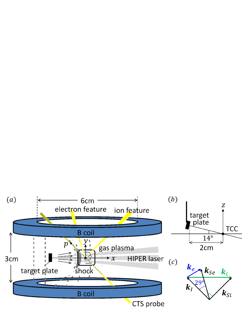
Figure 1: Experimental settings: (a) top view, (b) side view near the target, and (c) the relation among the wavenumbers of incident probe light ($\mbox{\boldmath$k$}_{I}$), scattered waves ($\mbox{\boldmath$k$}_{S}$), and plasma waves ($k$) for CTS measurement.

The experiment was carried out with Gekko XII HIPER laser facility at the Institute of Laser Engineering, Osaka University. Four beams of long pulse laser [energy of $\sim 700$ J at 1053 nm, Gaussian pulse with 1.3 ns duration and 2.8 mm spot, F/15 for each beam] irradiate an aluminum (Al) plate target with 2 mm thickness at $x=-2$ cm, behind the target chamber center (TCC), to create a high speed plasma flow normal to the target plate (Fig.1). 5 Torr nitrogen (N) gas filling the target environment was ionized due to the radiations from the laser-target interaction. The target position is more distant from the TCC than [12] ($x=-1.4\cos{14^{\circ}}$ cm) so as to capture longer time evolution of the system, although the structures associated with earlier time phenomena are outside the field of view. The ambient magnetic field parallel to the target surface was applied by using a Helmholtz coil (6 cm diameter of each coil and 3 cm inter distance) driven by a portable pulsed magnetic field generation system [13] so that the gas plasma was homogeneously magnetized. Two sets of capacitor banks, each consists of four condensers with 3 mF capacitance, were charged with $1.4$ kV and $\sim 3$ kA current was applied with a pulse duration of over 100 $\mu$s. This enabled us to apply $\sim 3.8$ T ambient magnetic field in the region of interest. The high speed target plasma carrying Biermann battery magnetic field acts as a magnetic piston to form a shock in the ambient gas plasma.

We measured spatio-temporal evolution of the system by using a 450 nm bandpass filtered SOP. Spatial information was obtained along the line parallel to the target normal, defined as $X^{\prime}$-axis inclined in the $x-z$ plane by $-14^{\circ}$ from the $x$-axis [Fig.1(b)]. CTS measurement for ion feature was conducted to obtain local plasma quantities at a particular time [14, 15]. The probe light (Nd:YAG laser, wavelength $\lambda_{0}=532$ nm, pulse duration 8 ns, laser energy 300 mJ) was injected along the $p$-axis which is inclined by $45^{\circ}$ from the $y$-axis in the $x-y$ plane [Fig.1(a)]. The detection system was placed in the direction of $-90^{\circ}$ from the $p$-axis, which mainly consists of a handmade triple-grating spectrometer [spectral resolution was 10 pm] and an intensified CCD camera (Princeton Inst., PIMAX4, gate width 5 ns quantum efficiency at $\lambda_{0}$ was 40%). In all the above coordinate systems, the origin is shared at TCC.

III Experimental results

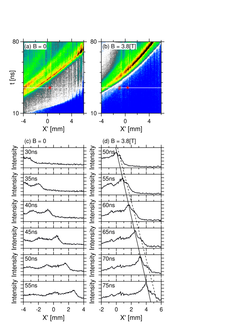
Figure 2: SOP data for the cases of (a,c) $B=0$ and (b,d) $B=3.8$ T. In (a) and (b) a vertical axis denotes an elapsed time from the laser shot. The color shows self-emission intensity normalized to the far upstream value. The intensity profiles at different times are plotted in (c) and (d). The solid and the dashed lines in (d) roughly trace the positions of the main peak and the plateau-like structure. CTS spectra at the red markers in (a) and (b) are shown in Figs.3(a) and 3(b), at the white marker is shown in Fig. 5(b), respectively.

The color images of the SOP data show that the peaks of high intensity emission propagated in the positive $X^{\prime}$ direction for $B=0$ [Fig.2(a)] and $B=3.8$ T [Fig.2(b)]. The propagation speed estimated at $X^{\prime}=0$ (TCC) was $\sim 270$ km/s in (a) and $\sim 210$ km/s in (b), respectively. In (a) a region where the emission intensity was slightly enhanced was extended in the right (upstream side) of the intensity peak. This structure was discussed by [12]. Hereafter, we call this as a precursor. In (b) the similar precursor with rather smaller spatial extent was seen only for $t<40$ ns. This could be the ’R2’ discussed in [12]. They interpreted this as the structure associated with gyrating N ions which are reflected by expanding target plasma in the early time phase. Another possible interpretation is that it is the structure associated with gyrating target ions. Using the value of 800 km/s as the initial target Al ion velocity (according to [12]), their gyro radius for $B=3.8$ T is $\rho_{Al}\sim 58/Z_{Al}$ mm, where $Z_{Al}$ is the average valence of Al ions. Since outermost electrons of an Al atom are easily excluded, it is natural to infer that $Z_{Al}\geq 3$ so that $\rho_{Al}<20$ mm. Hence, we conclude that the structure observed after $t>40$ ns is the one formed in a magnetized gas plasma not contaminated by the gyrating Al and N ions produced in the early time after the laser shot. The main intensity peak for $B=0$ [Fig.2(c)] has relatively simple and stable structure. In contrast, the intensity peak for $B=3.8$ T clearly has sub-structures and the details of the profile varies in time [Fig.2(d)]. In front of the main peak a local plateau-like structure is formed and the spatial size of the whole transition region widens in time during the period shown. The decay length of the whole transition region reaches $\sim 2$ mm, which is apparently larger than that ($\lesssim 1$ mm) of the main peak in the case of $B=0$.

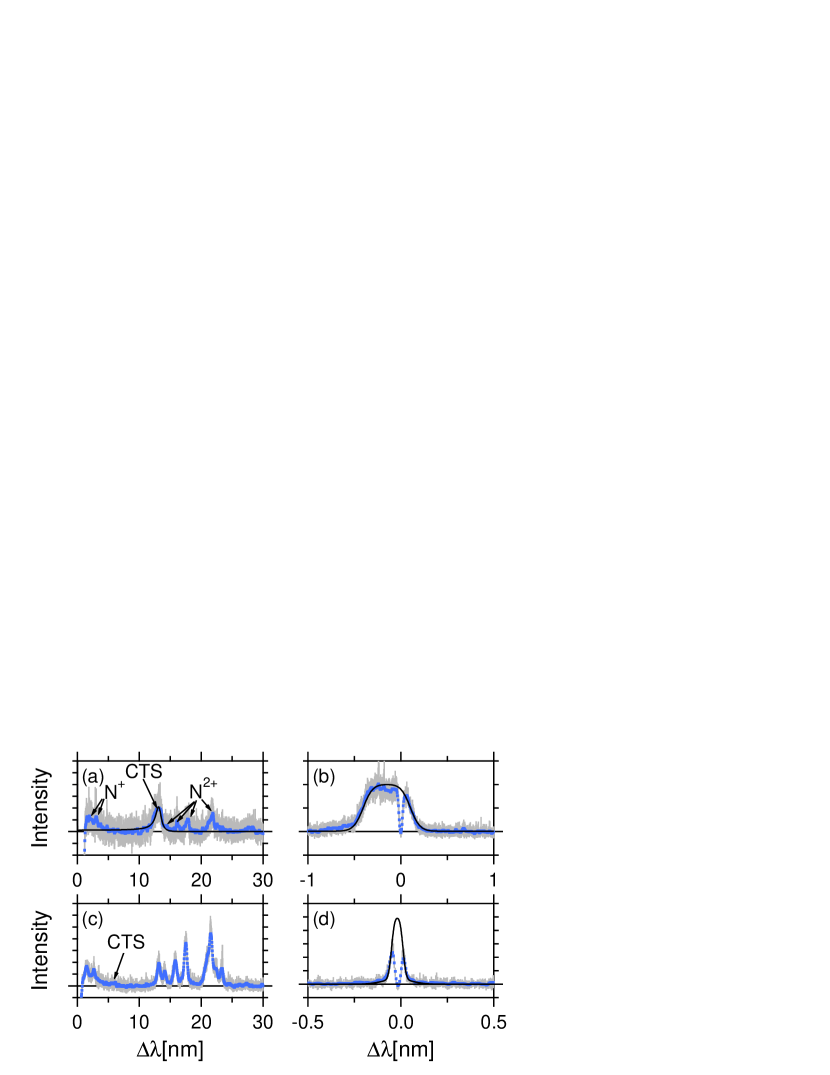
Figure 3: CTS spectra at $t=35(\pm 2.5)$ ns for (a,c) $B=0$ and (b,d) $B=3.8$ T. In the panels (a) and (b), the vertical and the horizontal axes indicate the position along the probe light ($p$-axis) and the wavelength shift, $\Delta\lambda$, from $\lambda_{0}$, the color denotes the arbitrary intensity of the scattered signal, respectively. The corresponding time integrated to obtain this data is shown as the red square in Fig.2(a) and (b). Assuming that a planar structure is propagating along the $X^{\prime}$-axis, a position along the $p$-axis is projected onto the $X^{\prime}$-axis as $X^{\prime}=-p\cos 14^{\circ}/\sqrt{2}$. The projection of the position is indicated as the red vertical bars in Fig.2(a) and (b). In the panels (c) and (d), the cross-section along the white line ($p=-0.5$ mm) in (a) and (b) is plotted. See the text in detail.

The CTS spectrum in the precursor for $B=0$ is shown in Fig.3(a). The vertical axis denotes the position, $p$, along the path of the probe light, while the horizontal axis indicates the deviation of wavelength from the probe light ($\lambda_{0}=532$ nm). The spectrum was obtained as a snapshot at $t=35(\pm 2.5)$ ns. The corresponding time domain (5 ns gate width) in the SOP data is indicated by the red square in Fig.2(a). In Fig.3(a), the signal is cut at around $\lambda_{0}$ to avoid stray light. An abrupt shift and broadening of the spectrum is observed in the region of $p>0$. The peak intensity occurs in slightly above $p=1$ mm, which may correspond to the peak in the red squared region in Fig.2(a). Note that the positive $p$ corresponds to the negative $X^{\prime}$. The deviation of the two axes may cause the slight discrepancy of the peak position. The cross-section of the spectrum in the precursor at $p=-0.5$ mm is shown in Fig.3(c). The blue dotted line denotes an arbitrary intensity averaged over $-0.51\leq p\leq-0.49$ mm at each wavelength, while the maximum and the minimum values in the region give the error bars indicated by the gray vertical lines. To fit the averaged data, we use the spectral density function written as

$$S(\bm{k},\omega)={2\pi\over k}\left|1-{\chi_{e}\over\epsilon}\right|^{2}f_{e0}\left({\omega\over k}\right)+{2\pi Z_{N}\over k}\left|{\chi_{e}\over\epsilon}\right|^{2}f_{N0}\left({\omega\over k}\right).$$ (1)

Here, $\omega$ and $k$ are the frequency and wavenumber of the density fluctuations of the plasma, $\epsilon$ and $\chi_{e}$ denote electric permittivity and electron susceptibility, $f_{e0}$ and $f_{N0}$ are the shifted-Maxwellian distribution functions of electrons and N ions, respectively. In the experiment the obtained signal is the convolution of $S(\bm{k},\omega)$ and $R(x)$, as $\hat{S}(\bm{k},\omega)=\int S(\bm{k},\omega^{\prime})R(\omega^{\prime}-\omega)d\omega^{\prime}$, where $R$ denotes the resolution of the spectrometer evaluated from the Rayleigh scattering. The electron density $N_{e}$ is determined by using the following relation between the intensities of the Thomson scattering and the Rayleigh scattering, $I_{T}/I_{R}=(N_{e}/N_{NG})(\sigma_{T}/\sigma_{R})(E_{T}/E_{R})(S_{N}/2\pi)$. $N_{NG}$ is the density of nitrogen gas, $\sigma$ the scattering cross section, $E$ the laser energy. The subscripts $T$ and $R$ denote Thomson and Rayleigh scatterings, respectively. $S_{N}$ is the total intensity integrated over $\omega$ of the second term of eq.(1). The black solid line is obtained using the above method as the best fit using electrons’ density $N_{e}\approx 1.4\times 10^{18}$ cm^-3, temperature $T_{e}\approx 240$ eV, drift velocity $v_{de}\approx 40$ km/s, ions’ temperature $T_{N}\approx 450$ eV, charge state $Z_{N}\approx 3.9$, and drift velocity $v_{dN}\approx 40$ km/s, respectively. These values are not very far from those obtained by [12] in the precursor at an earlier time and at a closer position to the target. Since $N_{e}/Z_{N}\approx 3.6\times 10^{17}$ cm^-3 is comparable to the density of N atoms contained in a 5 Torr gas ($\approx{\color[rgb]{0,0,0}3.2}\times 10^{17}$ cm^-3), the local plasma is considered to be fully ionized.

The CTS spectrum obtained at $t=35(\pm 2.5)$ ns for $B=3.8$ T is shown in Fig.3(b). A gradual broadening and shit of the spectrum occurs in $p>0.5$ mm. This region may correspond to the edge of the small precursor in Fig.2(b). The region of $p<0.5$ mm is regarded as an upstream gas plasma. The cross-section of the spectrum in this region at $p=-0.5$ mm is shown in Fig.3(d). Despite that the peak is cut, we fitted the blue dotted line to obtain the theoretical line shown by the black solid one by using $N_{e}\approx 4.5\times 10^{17}$ cm^-3, $T_{e}\approx 7$ eV, $T_{N}\approx 5$ eV, $Z_{N}\approx 1.3$, and $v_{de}=v_{dN}\approx 5$ km/s, respectively. Note that the above values of $N_{e}$ and $Z_{N}$ indicate that the 5 Torr gas was fully ionized. Using these values, the Alfvén velocity in the magnetized gas plasma upstream is estimated as $V_{AG}\approx 38.6$ km/s. Hence, the Alfvén Mach number corresponding to the propagation speed of the peak, $210$ km/s, is $M_{A}\approx 5.4$ indicating that the shock is supercritical. The upstream electron beta is $\beta_{e}\approx 0.1$.

IV Numerical simulation and discussions

To interpret the above experimental results, we numerically simulate the interaction between a target plasma and a gas plasma by using a one-dimensional PIC simulation. Recently, a method to simulate ambient and target plasma interaction is proposed by [16] and developed by [17]. Here, a similar but different method is used. Initially the system is filled with a uniform thermal gas plasma consisting of electrons and ions. The valence of gas ions is assumed to be $Z_{G}=1$, based on the CTS analysis ($Z_{N}=1.3$). The ion-to-electron mass ratio is $m_{G}/m_{e}=100$. The ratio of electron plasma frequency to cyclotron frequency is $\omega_{Ge}/\Omega_{Ge}=20$. The electron and ion betas are $\beta_{Ge}=\beta_{Gi}=0.1$ and their distribution function is Maxwellian. At $X^{\prime}=-2$ cm$/\cos 14^{\circ}$, a dense target plasma is injected during $0\leq\Omega_{Gi}t\leq 0.035$, where $\Omega_{Gi}$ is the cyclotron frequency of the gas ions. The target plasma is composed of electrons and hexavalent ions with ion-to-electron mass ratio $m_{T}/m_{e}=200$. The relative density of the target electrons to the gas electrons is $N_{Te}/N_{Ge}=9$ and the magnetic field carried by the target plasma is 6 times the ambient field. The injection speed of the target ions is $v_{in}=27v_{A}$, where $v_{A}$ denotes the Alfvén velocity in the gas plasma. The distribution function of target electrons is given by a full-Maxwellian in $v_{y}$ and $v_{z}$, and a half-Maxwellian in $v_{x}(>0)$. The temperature of the target electrons (and ions) is assumed to be $T_{e}=2m_{e}v^{2}_{in}$.

The Biermann battery effect through laser-target interactions are thought to generate $\sim 100$ T magnetic field at the target surface [12, 18, 19]. This field may decay away from the target. But it is difficult to infer precisely the magnetic field carried by the expanding target plasma. [12] performed two-dimensional radiation hydrodynamics simulation to estimate electron pressure and density of Al plasma ejected through laser-target interaction under the same condition (laser intensity and spot radius) as the experiment here. Their result shows that the Al plasma carries $\sim$ 100 (10) T magnetic field after 4 (8) ns near the target surface. Here, we assume that the magnetic field carried by the target plasma at the surface is 22.8 T. The dimensional effect of a toroidal field cannot be incorporated in the one-dimensional simulation so that we assume the magnetic field is perpendicular ($z$-direction) to the simulation axis. The duration of the injection of the target plasma is equivalent to $1.3$ ns which is the pulse duration of the HIPER laser. The injection speed roughly reads $\sim 900$ km/s, which is close to the value obtained by [12]. Although we use unrealistic mass ratio, the mass ratio of the target ions to the gas ions (=2) is approximately equal to that of the Al to N ions. We checked that the following results are little dependent on the ion-to-electron mass ratio and the frequency ratio, $\omega_{Ge}/\Omega_{Ge}$. The system size is $L=25v_{A}/\Omega_{Gi}$ ($\approx 32$ mm). The number of grids is 72,000 and the number of superparticles per cell is 256 for each species.

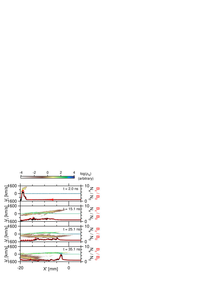
Figure 4: Early time evolution of ion phase space and the profiles of electron density (thick black line) and magnetic field (red line). The color scale denotes ion charge density, $\rho_{N}$.

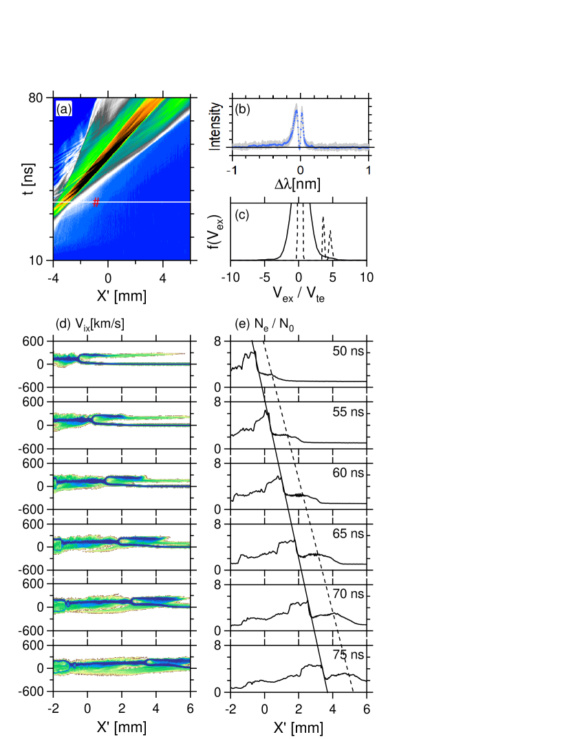
Figure 5: (a) Spatio-temporal evolution of $N_{e}$ in the PIC simulation with the strength of the Biermann field carried by the target plasma of 22.8 T. (b) Experimental data of CTS ion feature for $B=3.8$ T in the precursor at $p=1.36$ mm and $t=35$ ns. (c) Simulated electron (solid line) and ion (dashed line) distribution functions at the red sharp in (a). (d) Time evolution of ion phase space and (e) electron density profile. The rough positions of the main peak and the plateau are traced by the solid and the dashed lines, respectively.

Fig.4 shows early time evolution of the ion phase space distribution. Also plotted thick black line and red line denote the profiles of electron density and magnetic field, respectively. At $t=2.0$ ns, injected target ions are easily identified. While they gyrate around the ambient magnetic field in the gas plasma, they are elongated in the phase space due to their velocity dispersion ($t=15.1$ ns). After a quater of their gyro period ($t\approx 19$ ns), the target ions turned back and disappeared from the region around the TCC as seen in the panels of $t=25.1$ ns and 35.1 ns. Because of the short injection time and the velocity dispersion, the background gas plasma has not been compressed enough to form a shock before $t\sim 30$ ns. However, the gas ions are dragged (or accelerated) by the target ions during a quater of their gyro motion so that they have positive velocity in $v_{x}$. These gas ions are gradually accumulated and compressed to form a shock-like steepened density profile ($t=35$ ns). However, the density drops immediately behind the steepened region because no more sweep of the gas plasma occurs. We call this steepened structure as a developing shock.

The spatio-temporal evolution of electron density of the same field of view as the SOP data in Fig.2(b) is shown in Fig.5(a). It shares some common features with the SOP data. When $t<40$ ns, a region where the electron density is slightly enhanced is seen upstream of the main peak. After $t\sim 40$ ns, in front of the main peak, the region where the density is a little enhanced grows (green-colored). A developing shock lies at the sharp boundary just behind the green-colored region. Its propagation speed at $t=70$ ns is $v_{sh}\approx 153$ km/s ($M_{A}\approx 4.4$), while the propagation speed of the main peak in the experiment at the same time is $v_{sh}\approx 146$ km/s ($M_{A}\approx 3.8$) [Fig.2(b)].

As mentioned already, the developing shock shares some characteristics with a fully developed supercritical shock. In Fig.5(d) the developing shock stands at $X^{\prime}\approx-0.5$ mm when $t=50$ ns. After that, a main peak and a plateau are clearly seen in the electron density profiles in Fig.5(e). Although well developed uniform downstream has not been realized yet, the spatial extension of the post-ramp exceeds local ion inertial length as well as the thermal gyro radius of main local ion component. Non-negligible amount of incident ions are reflected at the front of the developing shock, while the plateau corresponds to the region where the reflected ions occupy, i.e., the foot, which extends as the reflected ions reach farther upstream. Accordingly, the density profile varies in time. This extension of the foot is similar to that of the plateau-like structure seen in the experiment [Fig.2(d)]. The simulated developing shock is self-reforming, although the reformation cycle has not completed by $t=80$ ns.

In the CTS spectrum in the precursor for $B=3.8$ T in the experiment [Fig.5(b)] the tail of the spectrum ($\Delta\lambda<-0.2$ nm) is clearly enhanced. This enhancement of the blue shifted signals implies the presence of electrons moving faster than the bulk toward the upstream. At the similar position and time in the simulation [red sharp in Fig.5(a)], the tail of the electron distribution function is enhanced for $V_{x}>0$ [Fig.5(c)]. Also plotted ion distribution function (dashed line) shows that some ions having positive velocity exist, indicating that some electrons are dragged by these ions. Therefore, it is inferred that the asymmetric CTS spectrum is related with the asymmetric electron distribution function. In the simulation the long time evolution of the electron distribution function in the foot after this is clearly correlated with the gyro motions of reflected ions. Hence, it is expected that the similar CTS spectrum in an experiment is obtained, if a well developed foot of a self-reforming shock is formed.

In the end of this section we make some comments. We have used some unrealistic values of parameters in the simulation. In particular, ion to electron mass ratios $m_{G}/m_{e}=100$ and $m_{T}/m_{e}=200$ are quite smaller than real ($m_{N}/m_{e}=25704$ and $m_{Al}/m_{e}=49572$). However, this seems not to lead significant influence on the results. We have scaled the simulation parameters in unit of ion quantities, i.e., the quantities normalized to $c/\omega_{pN}$, $\Omega_{N}$, and $v_{A}$ are chosen to match with the experimental data. This is of course justified only when we focus on the phenomena controlled by ion dynamics. On the other hand, there are a number of effects which may cause the discrepancy from the experiment. For instance, the spatial expansion of the developing shock may be a possible reason for deceleration of its speed [Fig.2(b)]. Non-uniformity of the system may also affect the properties of the observed developing shock in the experiment. For instance, the ionization level of the gas plasma may be different between the developing shock front and far upstream. All these effects should be taken into account for more accurate comparison between the simulation and the experiment.

As already mentioned, the estimate of Biermann battery effect is controversial. Although we used the value 22.8 T according to [12], there is also an estimate giving much smaller value of the self-generated magnetic field when the focal spot is large [20]. We have confirmed that the above result does not change very much even when the magnetic field carried by the target plasma is 1/30 times ($\approx 0.76$ T) that of the case we discussed. Fig.6(a) shows the spatio-temporal evolution of $N_{e}$ in the same format as in Fig.5(a). Although the details of instantaneous ion phase space [Fig.6(b)] and electron density profile [Fig.6(c)] at $t=50$ ns, for example, are different from Figs.5(d) and (e), the feature of propagation of the developing shock is similar. This is probably due to that the injected target plasma diffuses in space due to its velocity dispersion so that the impact of the magnetic field carried by the target plasma is not so significant. (Note that we slightly changed other parameters. The valence of target ions is 5, the relative density of the target electrons to the gas electrons is $N_{Te}/N_{Ge}=5$, and injection speed of the target ions is $v_{in}=24v_{A}$.)

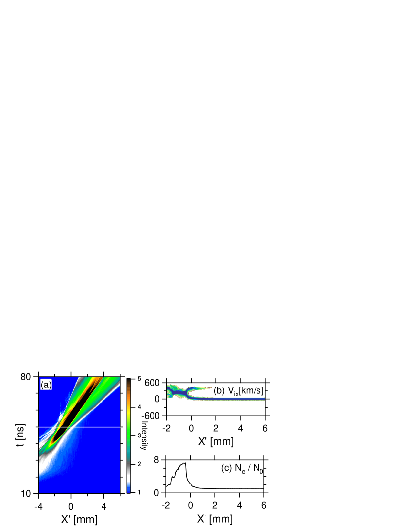
Figure 6: (a) Spatio-temporal evolution of $N_{e}$ in the PIC simulation with weaker magnetic field of 0.76 T carried by the target plasma. (b) Ion phase space and (c) electron density profile at $t=50$ ns.

V summary

In summary, a developing supercritical collisionless shock was produced in a uniformly magnetized gas plasma by using Gekko XII HIPER laser. A long time evolution of the system after $t>30$ ns were observed by the SOP and the CTS measurements. We successfully observed a developing shock formed in a homogeneously magnetized gas plasma without contaminated by the plasma produced in the vicinity of the solid target in the early time after the main laser shot. Although the observed developing shock has not developed to have uniform downstream, it possesses some characteristics of a supercritical shock. The Alfvén Mach number exceeds the critical Mach number ($\sim 3$) during the time observed. The width of the observed transition region varies in time and it is similar to the feature of the developing foot reproduced in the PIC simulation.

Finally, we emphasize utilities of the high-power laser experiment. We used an advantage that the information of space and time is separable to show that the spatial profile of a developing shock is time varying. There is also another advantage, although we have not focused it in this paper. While a remote sensing used in astrophysics observations enables us to capture global or macro scale structures of a phenomenon, local or micro scale structures of the phenomenon is usually unresolved. In contrast, in-situ observations in heliospheric physics can access detailed local information of particles and waves, while the global structure of the system at the same time is not accessible. That is, it is difficult in space to simultaneously measure global/macro and local/micro structures of a phenomenon. In the experiment one can simultaneously access multi-scale information. These indicate that the laser experiment can complement the conventional observations in space and can be a new basic tool of the research in high energy astrophysics, space plasma physics, and other related fields.