Simulating the Impact of Dynamic Rerouting on Metropolitan-Scale Traffic Systems

Abstract.

The rapid introduction of mobile navigation aides that use real-time road network information to suggest alternate routes to drivers is making it more difficult for researchers and government transportation agencies to understand and predict the dynamics of congested transportation systems. Computer simulation is a key capability for these organizations to analyze hypothetical scenarios; however, the complexity of transportation systems makes it challenging for them to simulate very large geographical regions, such as multi-city metropolitan areas. In this paper, we describe the Mobiliti traffic simulator, which includes mechanisms to capture congestion delays, timing constraints, and link storage capacity constraints. The simulator is designed to support distributed memory parallel execution and be scalable on high-performance computing platforms. We introduce a method to model dynamic rerouting behavior with the addition of vehicle controller actors and reroute request events. We demonstrate the potential of the simulator by analyzing the impact of varying the population penetration rate of dynamic rerouting on the San Francisco Bay Area road network. Using high-performance parallel computing, we can simulate a day of the San Francisco Bay Area with 19 million vehicle trips with 50 percent dynamic rerouting penetration over a road network with 0.5 million nodes and 1 million links in less than three minutes. We present an analysis of system-level impacts when changing the dynamic rerouting penetration rate and examine the varying effects on different functional classes and geographical regions. Finally, we present a validation of the simulation results compared to real world data.

1. Introduction

Active traffic management strategies using changeable message signs or broadcast media are regularly used by traffic management centers to present alternate routes to drivers when abnormal events occur on the roadways. Shifting traffic onto alternate routes maximizes the efficiency and capacity of the network and increases safety by reducing secondary vehicle accidents due to the unexpected congestion. With highways, parallel corridors that handle the rerouted traffic must be available with adequate capacity for rerouting to be successful. This requires traffic centers, with humans in the loop, to assess the situation, have knowledge of the parallel routes via predefined control strategies, and implement an active control plan. In the past five years, smart phone navigation apps have gained popularity and serve a similar role. These applications use their current understanding of congestion to compute new routes in which the travel time is shorter for the user of the device. The congestion information is generated by aggregating the speeds and locations of all of the devices that the app is monitoring. A road congestion estimate is created using road network information and other traffic information, such as historical traffic information, and combined with the current user’s destination. If the projected congestion of the user’s current route significantly impacts their expected travel time, the app may suggest a new route to the user with a shorter travel time. As such, these navigation applications are also serving as active traffic managers.

The introduction of these new active traffic managers makes it more difficult for researchers and government transportation agencies to understand and predict the dynamics of congested transportation systems. Traffic simulation is a key capability for these organizations to analyze different scenarios and predict the potential impacts of different infrastructure changes, policies, or control strategies. However, the complexity of transportation systems makes them extremely difficult to simulate at urban scale. As such, little is known about how to control and actively manage large scale road networks in the presence of significant congestion, particularly with the active management now being implemented by different agents, such as smart phone apps and traffic centers. We do know that providing information about congested states and having a variety of sources provide new travel routes will likely create unpredictable patterns and dynamic variation. Control strategies implemented through traffic management can include infrastructure modifications such as signal-phase-timing adjustments of signals to redirect traffic and expedite congestion mitigation. These control decisions are determined by estimating the impact of the rerouting action. To-date, these do not include rerouting that occurs as a result of drivers following an app’s routing information. This was made evident when during an evacuation event, drivers were venturing into dangerous situations with routes that were not informed by road closures associated with the event (CAL, 2017).

In the last two decades, transportation network simulation has increased in popularity for emulating driving behaviors, predicting traffic dynamics and predicting impacts of control strategies. Applied models can broadly be categorized into both equilibrium models, often referred to as traffic assignment models, and non-equilibrium models, often referred to as simulation models (Behrisch et al., 2008; Rojo, 2020). The simulation models complement traffic assignment, which is one of the essential tools that planners use for estimating congestion. With a reliable origin-destination demand matrix, an accurate traffic assignment generates optimized traffic-state predictions (Rojo, 2020). While equilibrium models have been very popular in the past due to mathematical clarity, their main drawback is the inability to capture the congestion-dependent evolution of a driver’s route (Kim et al., 2009). This limitation is overcome with non-equilibrium models that allow for modeling route guidance dynamics and unexpected events such as incidents or evacuation strategies (FHWA, 2021; Behrisch et al., 2008).

In order to predict the emergent traffic dynamics that result from congestion-dependent rerouting and unexpected events, we have extended our parallel discrete event simulation of large-scale traffic dynamics (Chan et al., 2018) with new dynamic vehicle rerouting capabilities. To understand the context of this paper, Figure 1 describes four different traffic models we have developed for large-scale network modeling, each with a different set of algorithms. Details of the baseline model can be found in our previous paper(Chan et al., 2018) and the quasi-dynamic traffic assignment model will be described in a forthcoming publication (Chan et al., 2021). In this paper, we focus on the second model with dynamic routing which we believe best captures realistic emergent traffic dynamics. Note that we acknowledge that there are a percentage of routes that are neither shortest free speed routes nor dynamically routed in the real world. We denote them as knowledge-based routes, representing routes that are arbitrarily chosen by a user, such as a route chosen to include a café stop en route to work. At this time, we do not model these types of routes; thus, all 19M routes are either shortest free speed routes or dynamically routed.

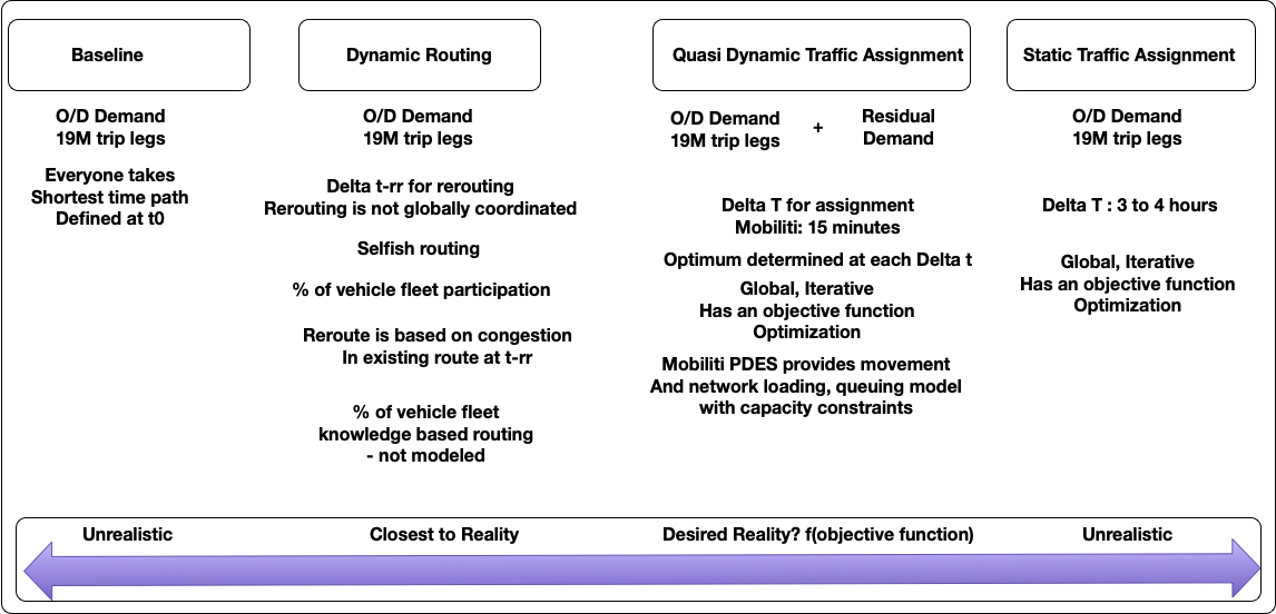
Figure 1. Four traffic models for large scale network modelling that can be employed for a wide array of transportation planning projects. While the first two employ non-equilibrium traffic assignment modelling, the last two use equilibrium based traffic assignment for route choice decisions.

The ultimate goal of active traffic management is to drive the system towards an optimized state, which is the focus of most traffic assignment algorithms. But in reality, reaching equilibrium is highly unlikely regardless of the attempted active management strategies. As such, a mechanism for simulating and analyzing hypothetical scenarios that will reveal emergent dynamics with prescribed dynamic routing algorithms would be extremely valuable for those designing active traffic management systems. With increased urbanization in cities today, understanding how to actively manage the dynamics on the road network is becoming increasingly urgent, not only from a loss in productivity perspective but from a fuel consumption perspective. Our research focus is to breakdown the computational barriers of simulating large scale road network dynamics in order to investigate the impacts of active traffic management strategies and reduce the multifaceted cost of the increasing congestion in our cities.

This paper presents a methodology for representing the transportation system with dynamic rerouting capabilities in a scalable actor-based parallel discrete event simulation (PDES) formalism. We include a description of the core link actor model and its constituent components that calculate vehicle traversal times, timing constraints, and storage capacity constraints. We also introduce vehicle controller actors that monitor congestion within the traffic system and handle dynamic reroute requests from simulated vehicles. We demonstrate that the resulting mesoscopic model achieves scalable computational performance for a large system (19 million vehicles over a network with 1 million links representing the San Francisco Bay Area), simulating a day of traffic with 50 percent dynamic rerouting penetration in three minutes on 512 cores of the NERSC Cori computer at Lawrence Berkeley National Laboratory (NERSC, 2018). We provide a rerouting parameter sensitivity analysis and discussion of the simulated impacts of varying the dynamic rerouting penetration rate on various transportation system metrics, and finally present a validation of the simulation results compared to real-world data sources.

2. Related Work

There has been much previous work in the area of transportation system modeling and simulation. Previous simulators can be broadly classified as macroscopic, mesoscopic, and microscopic based on the level of detail of the behavior of individual agents simulated. The level of behavior detail in the model typically also correlates to the size of the area under simulation – larger area simulations tend to use macroscopic models, while simulations focusing on small areas use more detailed microscopic models. DTA solvers and dynamic simulators such as MATSim (MATSIM, 2020), POLARIS (Auld et al., 2016), DTALite (Zhao et al., 2017), DynaMIT (Ben-Akiva et al., 2002), DynaSmart (Mahmassani, 1998), Aimsun (Casas et al., 2010), SUMO (Lopez et al., 2018), INTEGRATION (Rakha et al., 2012), BEAM (Sheppard et al., 2017), Ugirumurera et. al. (Ugirumurera et al., 2018), MANTA (Yedavalli et al., 2021), and many others fall along the spectrum of different modeling approaches, target problem scales, modeling fidelities, and output (e.g., traffic assignment versus simulation). The level of fidelity targeted by our Mobiliti simulator falls somewhere between microscopic and mesoscopic since it does not resolve lane-changing or vehicle following behavior, but it does resolve individual vehicle movements and rerouting decisions.

There is a large body of previous work in the area of parallel discrete event simulation (PDES, see (Fujimoto, 1990) for an overview). In particular, seminal work by Chandy and Misra (Chandy and Misra, 1979), Bryant (Abrams, 1989), and Jefferson (Jefferson, 1985) laid the groundwork for parallel discrete event simulation, which was shown to run efficiently on supercomputers (Barnes et al., 2013; Bauer Jr. et al., 2009). Previous traffic simulators that utilize PDES include those by Perumalla (Perumalla, 2006) and Yoginath (Yoginath and Perumalla, 2009), who used optimistic PDES for modeling traffic grids, though they evaluated their system on smaller-scale synthetic grid networks and used a different mechanism to mediate congestion among vehicles. Thulasidasan et. al. (Thulasidasan and Eidenbenz, 2009) also modeled road networks using queue-based parallel discrete event simulation, but they did not include adaptive vehicle rerouting behavior in their model, where vehicles can respond to congestion by rerouting in the middle of (rather than just at the beginning of) their trip. Furthermore, our paper includes a description of the design and implementation of a dynamic vehicle rerouting system with a parameter sensitivity analysis for vehicles and controllers at large scale.

In the area of dynamic re-routing, research by Liang and Wakahara (Liang and Wakahara, 2014) showed how proactive dynamic re-routing could reduce average travel time for congested road networks using the SUMO micro simulator on a medium-sized area of London (3,002 links and 332 nodes with 954 vehicles). Zhao et. al. (Zhao et al., 2017) gave a theoretical analysis of the dynamics and stability of equilibrium with travelers that reroute depending on cost difference, and demonstrated their results on some small networks (up to 31 nodes and 40 links with three OD pairs). Similarly, (Wang et al., 2021) provides a theoretical treatment of distributed multi-agent route selection problem with incentives, with numerical examples of their approach on the Sioux Falls road network (24 nodes). In (Tseng and Ferng, 2021), the authors utilize SUMO and OMNeT++ to model an area of Brooklyn with 380 nodes and 474 links, with a traffic demand of 2,500 vehicles. Their approach is similar to ours (albeit on a smaller network) in that they utilize a distributed cloud-based vehicle control system, where sensors detect congestion, and routes are suggested to avoid the congestion. In (Kim et al., 2020), the authors utilize a combination of SUMO, Veins, and OMNeT++ tools to analyze the impact of rerouting on a 2x2 grid map (9 nodes, 24 links). In (Qurashi et al., 2020), the authors describe a vanpool scheduler architecture for dynamic rerouting. They evaluate their approach on a network of the Munich city center, where the focus is more on responding to stochastic vanpool requests rather than dynamic congestion effects. In (Kucharski and Gentile, 2019), they investigate the information comply model to simulate how drivers can react to information about an event and evaluated their approach on a network with approximately 1000 links. There has also been related work in the area of route selection in the context of dynamic traffic assignment (e.g., (Auld et al., 2019)). Dynamic traffic assignment approaches typically model converged dynamic driver behavior adapted to daily congestion patterns, rather than more reactive dynamic rerouting scenarios that explore how traffic can respond to unexpected events. Our approach differs from these previous works in that we leverage high-performance computing techniques to simulate the effect of dynamic rerouting on much larger road networks (on the order of hundreds of thousands to millions of links) with tens of millions of vehicle trips per day to resolve system-wide impacts on large urban regions.

Traffic simulation systems use a variety of models and algorithms based on the problem that is being addressed. Geographical scale, modeling fidelity, time horizon, and desired output data all lead to a varied landscape of simulation tools. However, to the best of our knowledge, this paper presents the first simulation framework to model the impact of dynamically rerouting vehicles in a large urban region at scale with millions of nodes and links and millions of vehicles in short execution times, as well as present a rerouting parameter sensitivity discussion and detailed model validation analysis.

3. MOBILITI SIMULATION

Mobiliti is a distributed-memory, parallel simulation framework that runs on high-performance computing platforms. It uses an actor-based model and optimistic parallel discrete event simulation (i.e. Time Warp (Jefferson, 1985)) to model the traffic congestion in the network and the rerouting behavior of vehicles in the system. The overall workflow of the simulator is presented in Figure 2, which shows a concise subset of the inputs, stages of initialization and simulation, and outputs produced by the simulator. During the simulation phase, the links are modeled as actors and the vehicles are represented as events that are passed from link to link as they travel through the road network. Figure 3 illustrates the representation of network links as actors passing vehicle events between them.

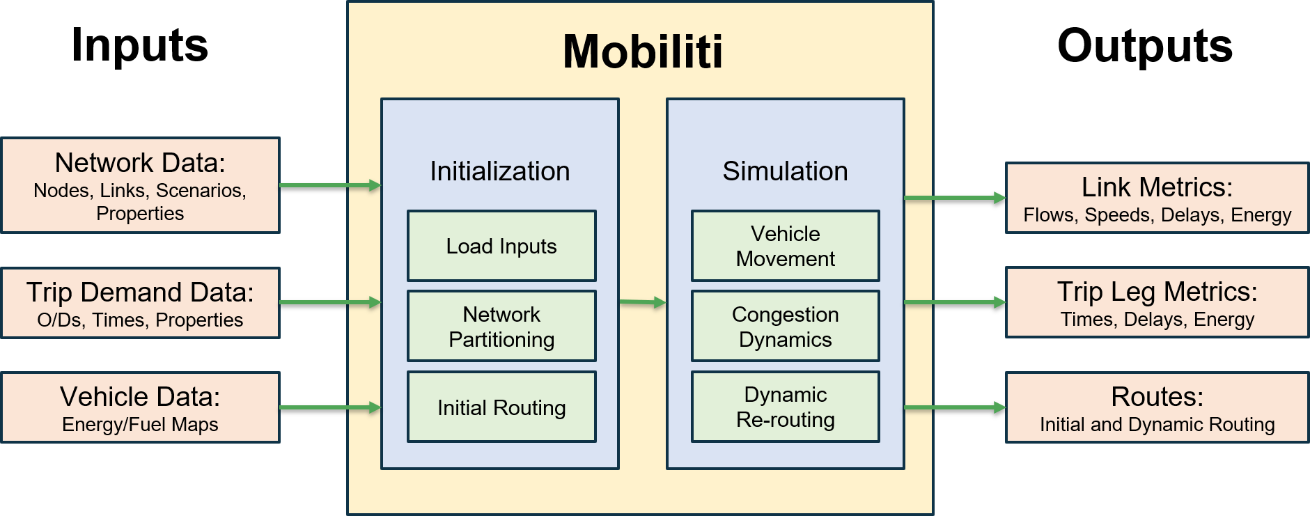
Figure 2. The Mobiliti simulator workflow. A subset of the inputs and outputs are shown along with a subset of the software stages and modules contained within Mobiliti.

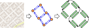
Figure 3. The Mobiliti simulator represents the road network as a collection of link actors that send events to each other representing individual vehicles traversing the network. Vehicles are initialized at their origin nodes and propagated from link to link until they reach their destination. Links are responsible for computing the vehicles’ traversal times based on the link’s congestion model.

For background on the simulator’s implementation, please see our previous paper  (Chan et al., 2018). This section describes relevant updates to the simulation that improve the accuracy of the link model and enable vehicle dynamic rerouting capabilities. Specifically, we have added mechanisms inside the link actor to enforce more accurate link timing constraints and storage capacity constraints, and we have added a new set of vehicle controller actors that can be queried by vehicles to compute better routes using the current congested state of the network.

3.1. Computational Link Model and Representation

When a vehicle event arrives at a link actor at time $T_{0}$, the link actor is responsible for determining the simulated time that the vehicle transitions to the next link on its route. As shown in Figure 4, the link actor utilizes three sub-models to determine the vehicle’s transition time: a flow-based congestion delay model, a link timing model, and a storage constraint model that limits the occupancy on each link based on physical dimensions.

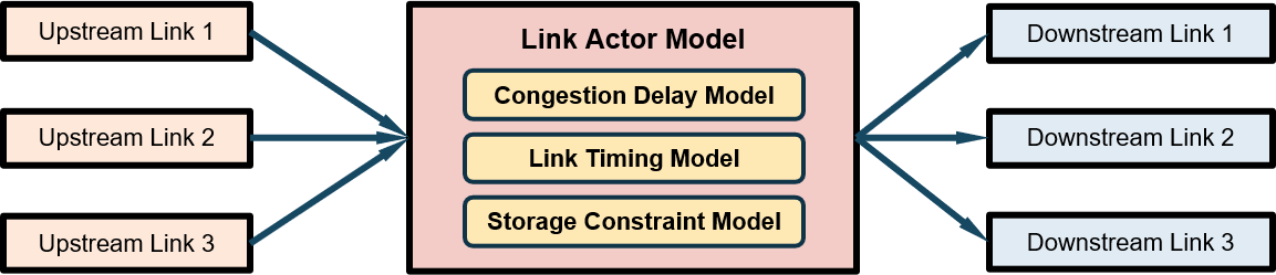
Figure 4. Each link in the simulation is modeled with a Link Actor object that utilizes three sub-models to resolve the various dynamics of the road network.

The flow-based congestion delay model (Figure 5) uses characteristics of the link (such as the designated flow capacity) and the current activity on the link to estimate the time $\Delta T_{1}$ it takes for vehicles to traverse from the beginning to the end of the link. The resulting time $T_{1}=T_{0}+\Delta T_{1}$ represents when the vehicle reaches the end of the link; however, the vehicle may be delayed further before actually transitioning to the next link in its route due to additional timing and storage capacity constraints.

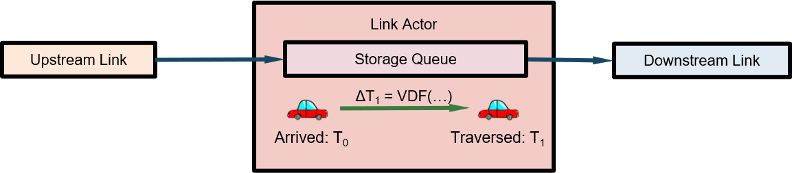
Figure 5. The Congestion Delay Model consists of a vehicle delay function (VDF) that uses link characteristics (such as designated flow capacity) and current activity (such as flow rate) to compute estimated traversal times $\Delta T_{1}$.

The link timing model computes the times at which vehicles may legally traverse from the current link to the next. Separate internal queues are maintained for each maneuver through the intersection (i.e. each downstream link sequence) so that vehicles utilizing different signal phases can be handled independently. Figure 6 shows a diagram of the internal queue data structures each link actor utilizes to track the vehicles currently occupying it. The timing model for each link is fully parameterized so that different, coordinated signal timing plans can be used at multiple intersections in the simulation.

The link timing model actually ensures two things: 1) that vehicles do not transition from link to link at a rate that is faster than physically allowable (determined by the product of vehicle speed, density, and number of lanes), and 2) that vehicles obey the traffic signals (if there is one at this link). For each queue within the link actor, it keeps track of the previous vehicle’s transition time so that the next vehicle traversal maintains a minimum time spacing between transitions to the downstream link. Furthermore, if the intersection has a traffic signal, vehicles may only transition to the downstream link when the corresponding signal phase is green. When combined with the minimum spacing requirement, each green phase is modeled as a time interval with a fixed number of consecutive vehicle slots during which no more than that fixed number of vehicles may transition to the downstream link. For each vehicle, the timing model assigns a time $T_{2}=T_{1}+\Delta T_{2}$ that obeys the above constraints. For our current experiments, we utilized the timing model only to enforce the maximum rate for vehicle arrivals at each link since we do not currently have comprehensive signal timing and phase information for the San Francisco Bay Area network. However, the link capacity parameters used in the vehicle delay functions in the simulator should reflect the lower capacity constraints for links that contain signals.

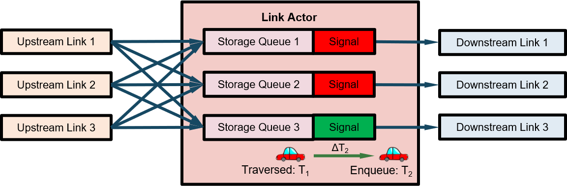
Figure 6. The Link Timing Model assigns transition request times based on minimum vehicle spacing requirements and signal phase timing information.

Finally, the storage capacity constraint ensures that links do not allow more vehicles to occupy the link than there is physical space. The storage capacity constraint is mediated by a system of EnqueueRequest and ArrivedNotice events between the upstream and downstream links. After a vehicle’s preliminary link traversal time $T_{2}$ is calculated using the congestion delay and timing models, the link actor sends a vehicle enqueue request event to the corresponding downstream link actor at its requested transition time $T_{2}$. However, the vehicle remains in the upstream link’s storage queues until a response is received. Only when there is sufficient capacity on the downstream link to accept the incoming vehicle does the downstream link send an ArrivedNotice event to the upstream link (at time $T_{3}=T_{2}+\Delta T_{3}$) to notify the upstream link that the vehicle has made the transition. At that time, the upstream link may remove the vehicle from its storage queues, potentially freeing up space to send another ArrivedNotice event further upstream. Figure 7 illustrates the described protocol that coordinates the transition of vehicles between connected link actors. The final traversal time for the vehicle over the link is $\Delta T=\Delta T_{1}+\Delta T_{2}+\Delta T_{3}$.

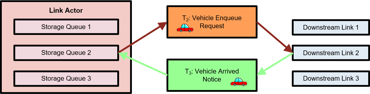
Figure 7. The Storage Capacity Constraint Model ensures that vehicles only transition from the upstream link to a downstream link if the downstream link has sufficient physical storage capacity to accept the vehicle.

3.2. Dynamic rerouting design

This section details the simulation mechanism that controls how vehicles dynamically reroute in response to system congestion. The subset of vehicles that have dynamic rerouting enabled (e.g. those with navigation devices) is specified at program initialization, determining the population rerouting penetration rate. In order to simulate dynamic rerouting behavior in the system, we implemented an additional set of actors and events that are responsible for coordinating when and how vehicles reroute. These include VehicleController actors, LinkStatusUpdate events, and vehicle RerouteCheck events. These new actors and events are described in the following sections, and relevant parameters are summarized in Table 1.

Table 1. Tunable dynamic rerouting parameters

Parameter	Description	Nominal Value
$t_{\text{lsu}}$	Absolute link status update threshold	60 s
$r_{\text{lsu}}$	Relative link status update threshold	1.0
$t_{\text{check}}$	Reroute check interval	300 s
$t_{\text{delay}}$	Absolute reroute threshold	120 s
$r_{\text{delay}}$	Relative reroute threshold	0.2

3.2.1. VehicleController actors

VehicleControllers are a new class of actors that can be queried by vehicles to check whether the vehicle should change its route based on current congestion conditions to get to its destination more quickly. There are multiple controllers instantiated throughout the road network, and since we already partition the road network across simulator ranks (threads) for parallel execution, we use the same partitioning for the VehicleControllers in our experiments. While each individual controller is only responsible for servicing requests originating from vehicles within its partition, it maintains current congestion data across the entire network, so newly computed routes take the state of the whole system into account. Figure 8 shows an example of how the San Francisco Bay Area road network could be partitioned into sub-networks. A distinct VehicleController actor is assigned to each sub-network shown in different colors. When vehicles check whether to reroute, they contact the VehicleController assigned to the vehicle’s current road partition. This method preserves geospatial locality within the model and also has good computational behavior since the VehicleControllers responsible for routing calculations are parallelized across compute resources in a similar manner that link actors are parallelized.

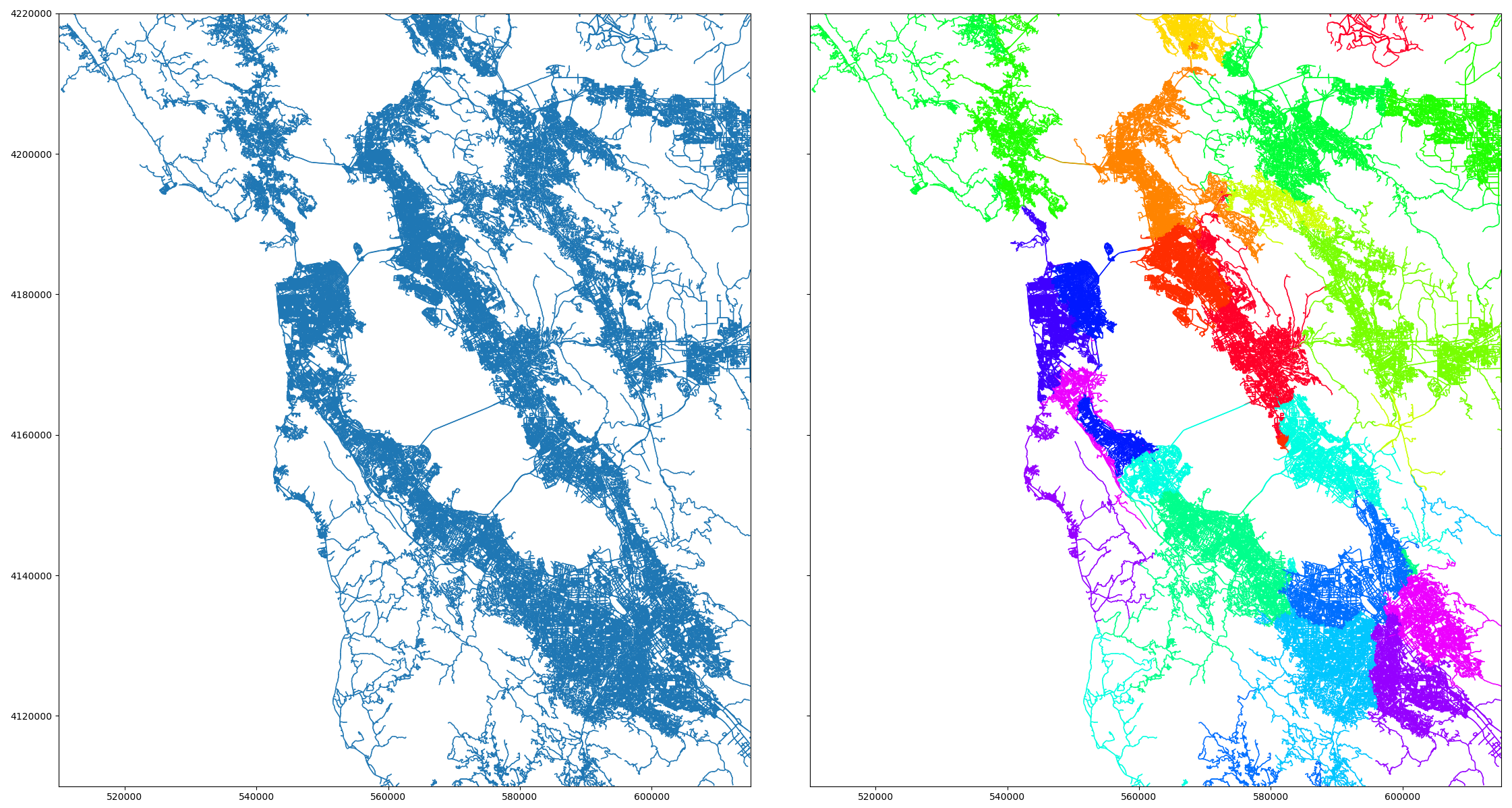
Figure 8. An example partitioning of the SF Bay Area road network into sixteen subgraphs. Mobiliti partitions the road network into subgraphs and assign one to each computational rank in the simulator. The partitions are load balanced to enable parallel scalability, and each partition is assigned its own VehicleController actor to service rerouting requests from vehicles currently in the partition.

3.2.2. LinkStatusUpdate events

In order for the VehicleControllers to have an up-to-date picture of current congestion conditions to make rerouting decisions, each link has a new sub-component that sends updates about its current congestion status to the VehicleControllers. Figure 9 illustrates an example where two link actors send status updates to a VehicleController, which then updates its knowledge of the road network’s congested link traversal times.

Every time a vehicle departs a link $l$, the link actor broadcasts an update to all VehicleControllers with its new congested traversal time if it differs from the previously sent traversal time by at least $\min(t_{\text{lsu}},r_{\text{lsu}}\cdot t_{f}(l))$, where $t_{\text{lsu}}$ is an absolute threshold, $r_{\text{lsu}}$ is a relative threshold ratio and $t_{f}(l)$ is the link’s freespeed traversal time. By allowing some deviation, the thresholds prevent links from sending excessive status updates while ensuring that the values used by the VehicleControllers for rerouting are still close to the current value experienced on the link. By making the thresholds tighter, we can increase the frequency that LinkStatusUpdate events are sent to the VehicleControllers, potentially improving rerouting accuracy at the cost of processing more update events. The sensitivity to these threshold parameters is explored in Section 3.3. Finally, each link actor that has active traffic periodically sends a heartbeat update to the vehicle controllers to indicate that it is still servicing traffic at a given speed. When a vehicle controller has not heard from a link in more than the heartbeat period, it knows the link has not had any traffic, and thus it can purge stale congestion data about the link from its database.

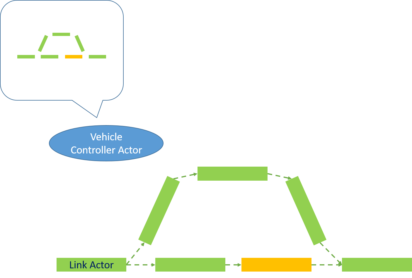
(a) Initial controller and link states

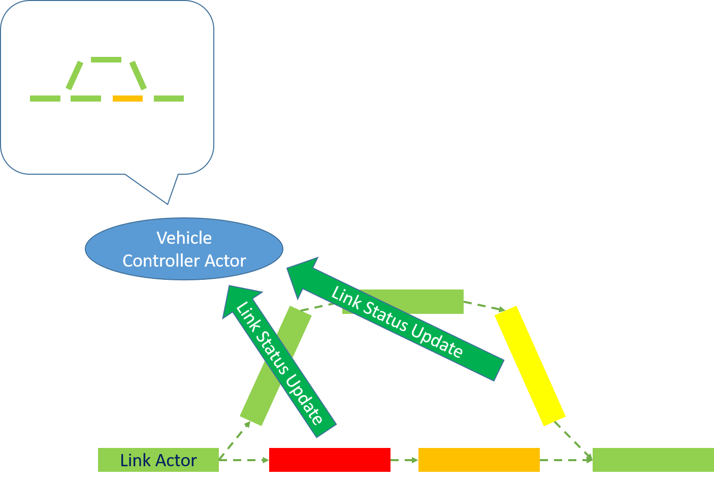
(b) LinkStatusUpdate events

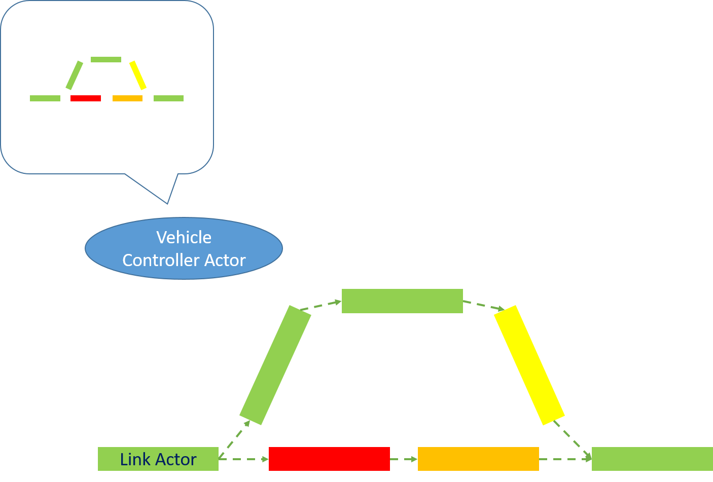
(c) Updated controller state

Figure 9. In (a), the VehicleController actor’s knowledge of the congestion on the links is up to date. When the congestion on a link changes during simulation, the link actor sends LinkStatusUpdate events to the VehicleController actors to notify them of its current condition. Figure (b) illustrates an example where two links experience increased congestion and send updates to the VehicleController actor. The controller then updates its knowledge of the graph (c) and uses this updated information to calculate routes for rerouting vehicles.

3.2.3. RerouteCheck events

When a vehicle arrives at a link, a vehicle can query the local VehicleController with a message that contains the vehicle’s current path $p$ (sequence of links) from its present location to its destination. The controller estimates the total congested time $t_{c}(p)$ on the vehicle’s path to its destination using its knowledge of current network congestion. If the delay on its path $d(p)=t_{c}(p)-t_{f}(p)$ exceeds a threshold $\max(t_{\text{delay}},r_{\text{delay}}\cdot t_{f}(p))$, where $t_{\text{delay}}$ is an absolute threshold, $r_{\text{delay}}$ is a relative threshold ratio, and $t_{f}(p)$ is the freespeed traversal time on path $p$, then the controller calculates a new shortest path $p^{\prime}$ from the vehicle’s current location to its destination. If the new path time $t_{c}(p^{\prime})$ improves the vehicle’s expected arrival time by more than $\max(t_{\text{delay}},r_{\text{delay}}\cdot t_{c}(p)$, then the vehicle accepts the new path $p^{\prime}$; otherwise, it continues on its existing path $p$. We assume a 100 percent compliance rate with the route suggestion given by the VehicleController (with no delay) since our simulator does not include human behavior models at this time. A lower compliance rate may be approximated by adjusting the population rerouting penetration rate accordingly. Finally, in order to prevent excessive reroute queries, the vehicle only sends a RerouteCheck event if it has been more than $t_{\text{check}}$ seconds since its last check. For our experiments, the VehicleController actors are homogeneous, simulating a unified network control agency. They could also be configured heterogeneously to simulate the impact of having multiple companies with different (imperfect) network information servicing vehicle reroute requests. This is a subject for future investigation.

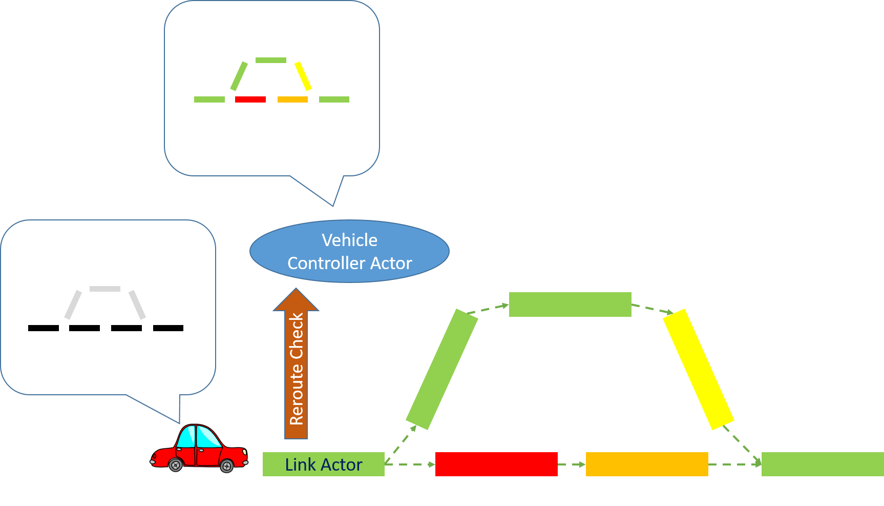
(a) Vehicle arrival and RerouteCheck query

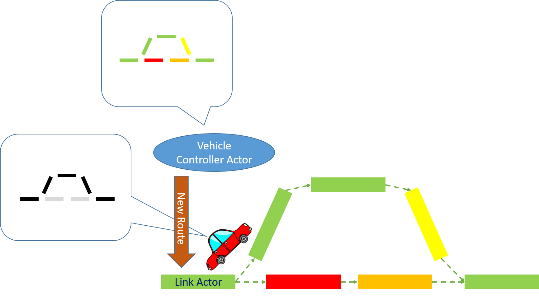
(b) RerouteCheck response with new route

Figure 10. Example RerouteCheck event for dynamic rerouting a vehicle based on current congestion conditions. Since the vehicle’s original route is congested, the controller sends an alternate route around the congestion, which the vehicle then takes.

3.3. Model Parameter Selection and Sensitivity

The various parameters described above and summarized in Table 1 control various aspects of the system’s rerouting behavior and can be tuned to explore how the system would hypothetically behave with different parameterizations. The parameters can be grouped into three categories: 1) $t_{\text{lsu}}$ and $r_{\text{lsu}}$ control the frequency of link status updates, where lower values result in more update messages and provide the controllers with more accurate information; 2) $t_{\text{check}}$ controls the frequency that vehicles contact the controllers to see if they should reroute, where lower values result in more requests; and 3) $t_{\text{delay}}$ and $r_{\text{delay}}$ control how aggressive the controllers are at rerouting vehicles, where lower values result in additional reroutes in situations with smaller time saving benefits.

In order to understand the sensitivity to these parameters, we conducted parameter sweeps for each of these three groups, where we simultaneously varied the values of the parameters in each group, while keeping the other parameters constant to isolate the impact of each group of parameters. Table 1 shows the baseline parameter values. In the first parameter sweep shown in Figure 11, we varied the link status update thresholds: $t_{\text{lsu}}$ (on the x-axis) and set $r_{\text{lsu}}=t_{\text{lsu}}/60$. As expected, the number of link status updates sent (a) decreases significantly as the thresholds increase; however, the impact on the number of trip leg reroutes (b) and on the total system delay (c) is relatively small, indicating that there is little benefit from sending very frequent updates, and that the vehicle controllers do a satisfactory job even with coarse information.

(a) Link Status Updates Sent

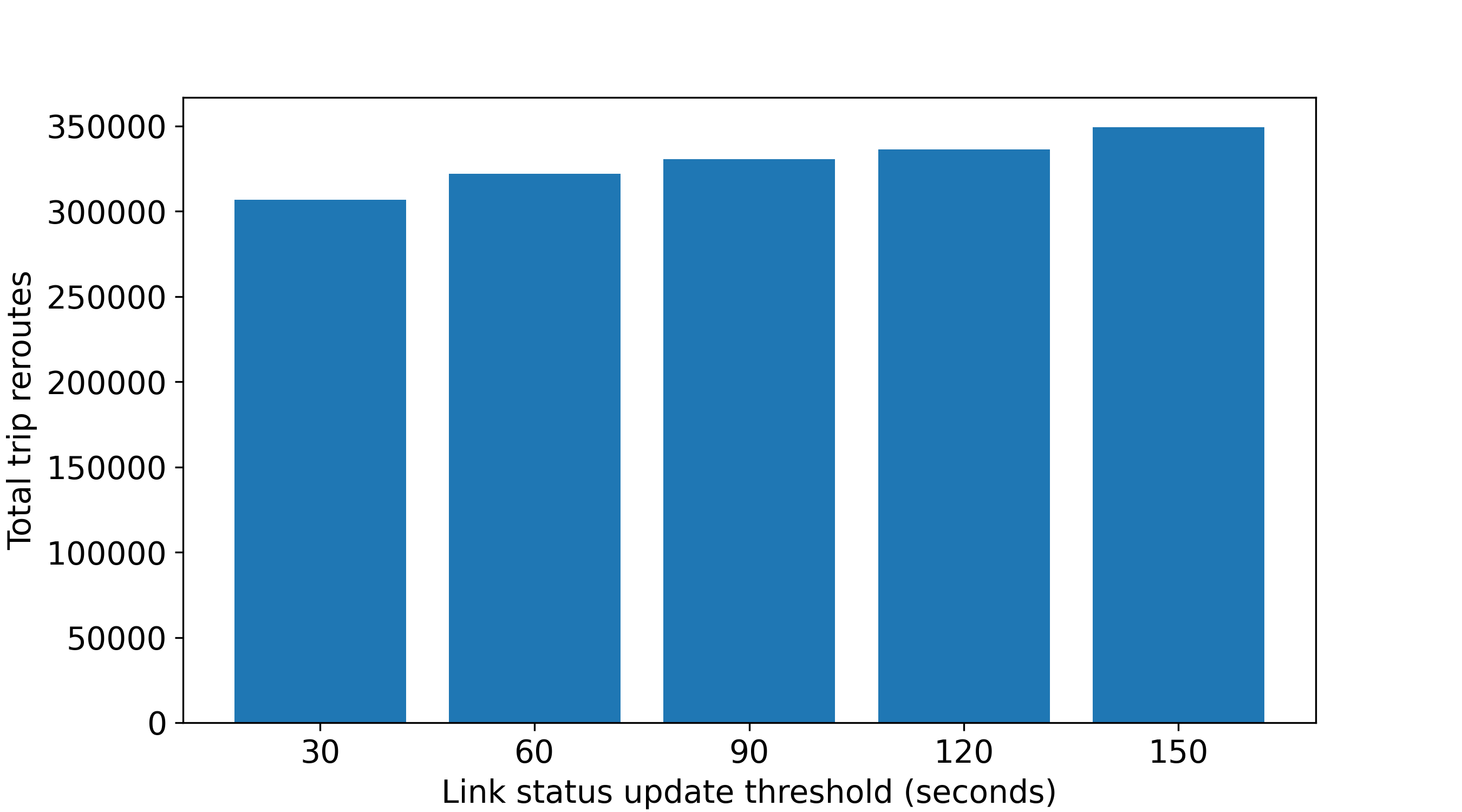
(b) Trip Leg Reroutes

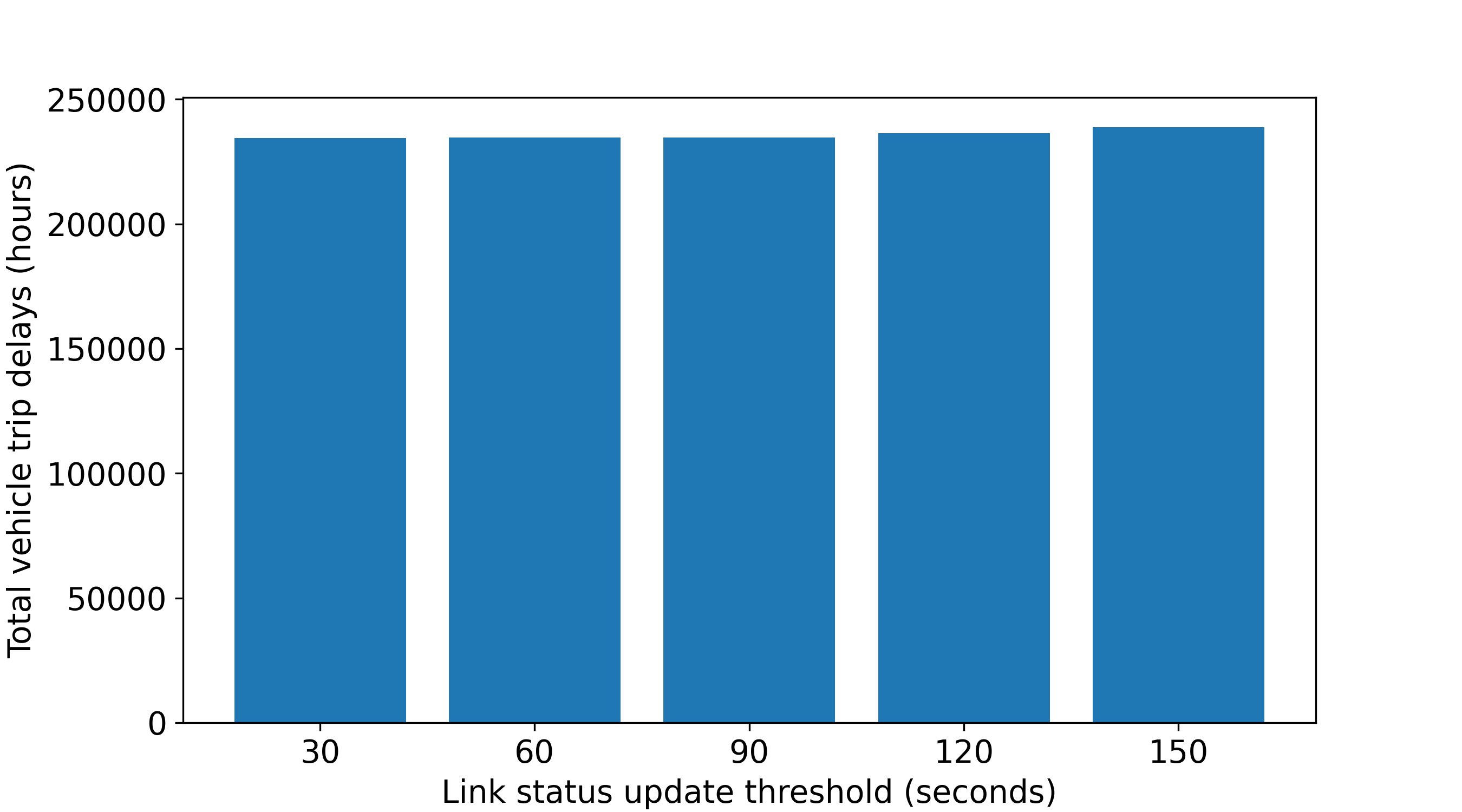
(c) Total (System) Vehicle Delay

Figure 11. Parameter sensitivity sweep for link status update thresholds. X-axis is the absolute link status update threshold $t_{\text{lsu}}$, where $r_{\text{lsu}}=t_{\text{lsu}}/60$.

In the second parameter sweep shown in Figure 12, we varied the minimum time interval between a vehicle’s reroute check queries: $t_{\text{check}}$ (on the x-axis). As $t_{\text{check}}$ increases, vehicles check whether they should reroute less frequently, but we observe that the total number of trip reroutes (b) declines only modestly. This is because the vast majority of vehicles that reroute only have to check and switch to a better route once, and then it typically sticks to the new route (e.g., with 60% rerouting penetration, 98.2% of rerouted trips only reroute once during its journey). Thus, increasing the time interval between checks mostly results in a small delay in the timing of a switch to a better route. As a result, the impacts on the number of link status updates (a) and total system delay (c) are also relatively minor.

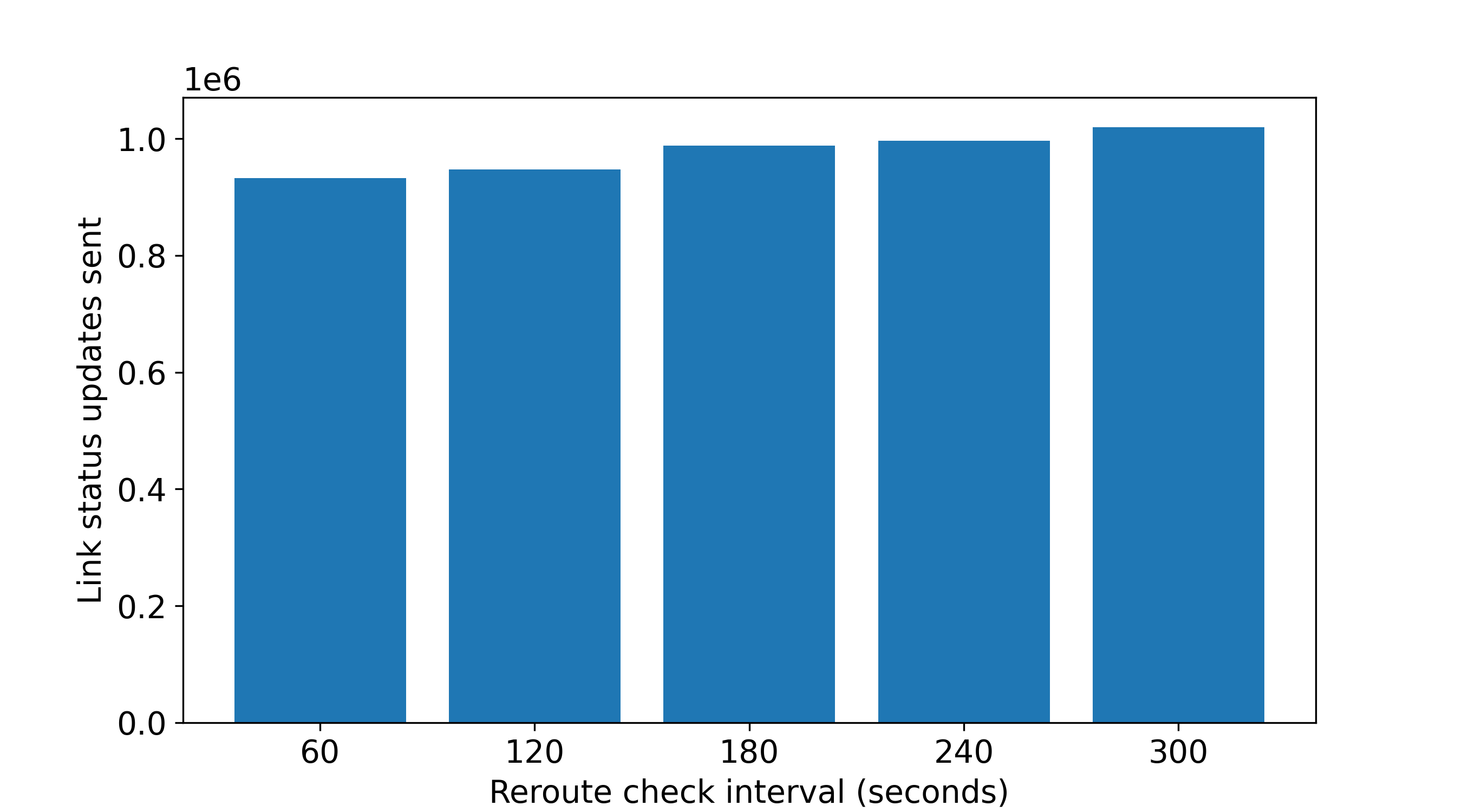
(a) Link Status Updates Sent

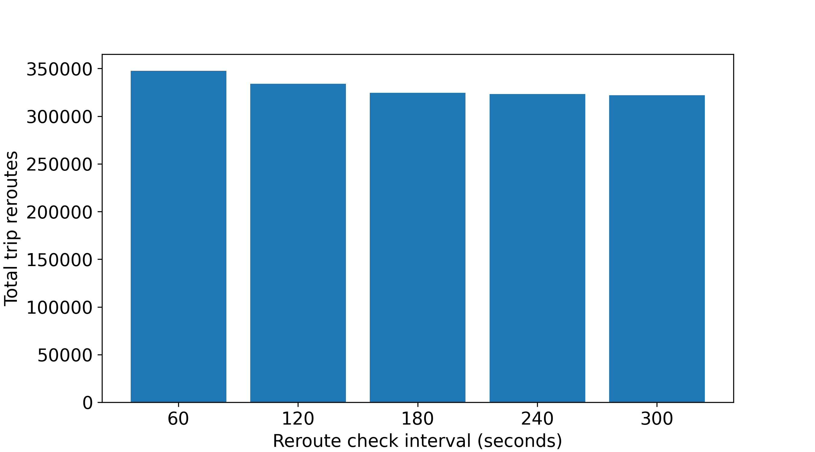
(b) Trip Leg Reroutes

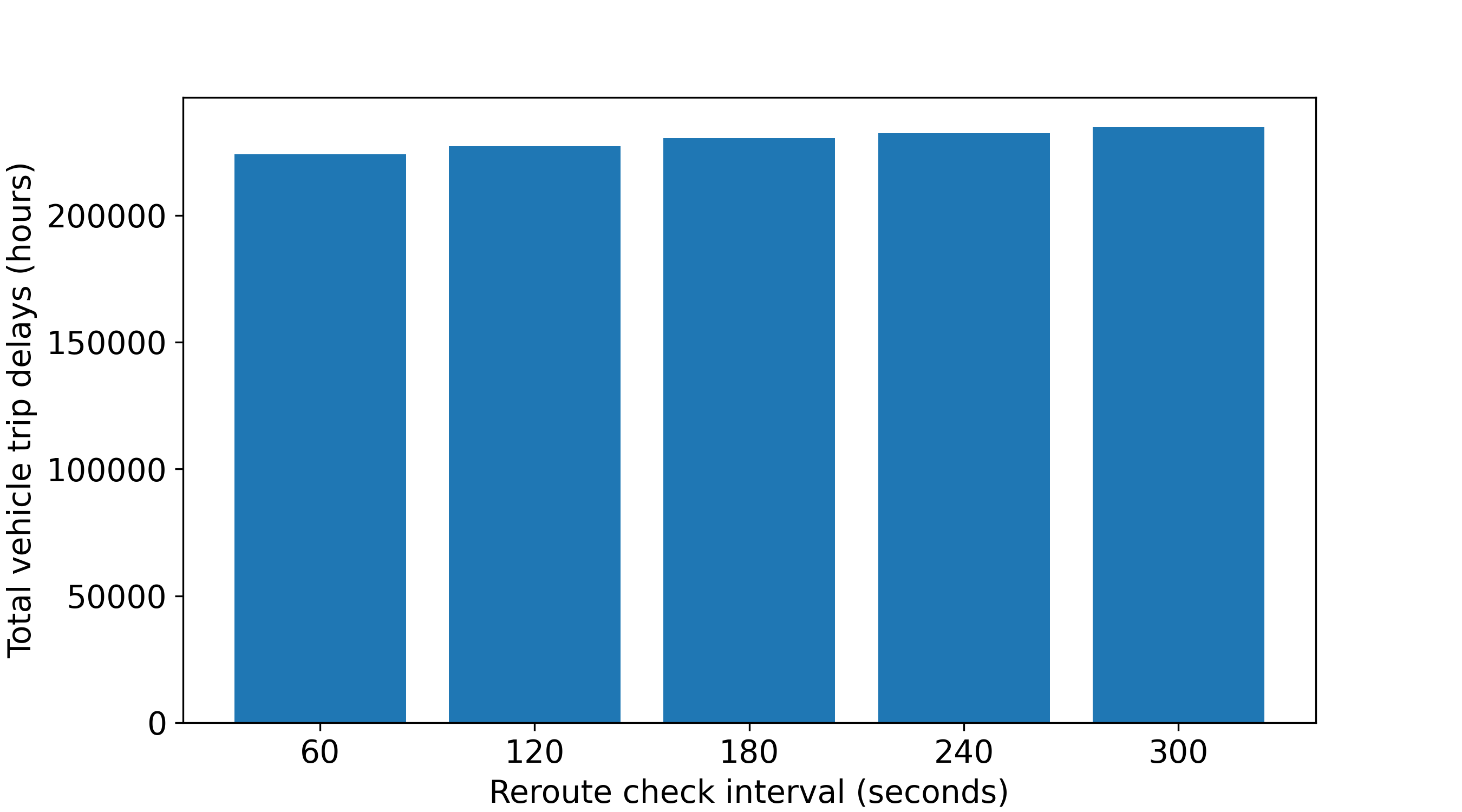
(c) Total (System) Vehicle Delay

Figure 12. Parameter sensitivity sweep for rerouting check frequency. X-axis is the reroute check interval $t_{\text{check}}$.

In the third parameter sweep shown in Figure 13, we varied the delay thresholds for when a vehicle should reroute: $t_{\text{delay}}$ (on the x-axis) and set $r_{\text{delay}}=t_{\text{delay}}/600$. As $t_{\text{delay}}$ increases, the vehicle controllers are less aggressively rerouting vehicles, keeping them on their original paths until their current path congestion is higher and their best alternative route saves them more time. This is directly seen in the middle graph as the total number of trip reroute requests decreases significantly as the thresholds increase. The number of link status updates (a) increases due to more dynamic variation in congestion, as the controllers are less effective at balancing traffic among available alternatives. The total system delay (c) increases since more vehicles are staying on less optimal routes, thus increasing their delay. While the smallest threshold resulted in the best system efficiency, it is debatable whether using a very low delay threshold in the real world with human drivers is desirable because of the cognitive cost in asking a driver to alter their route.

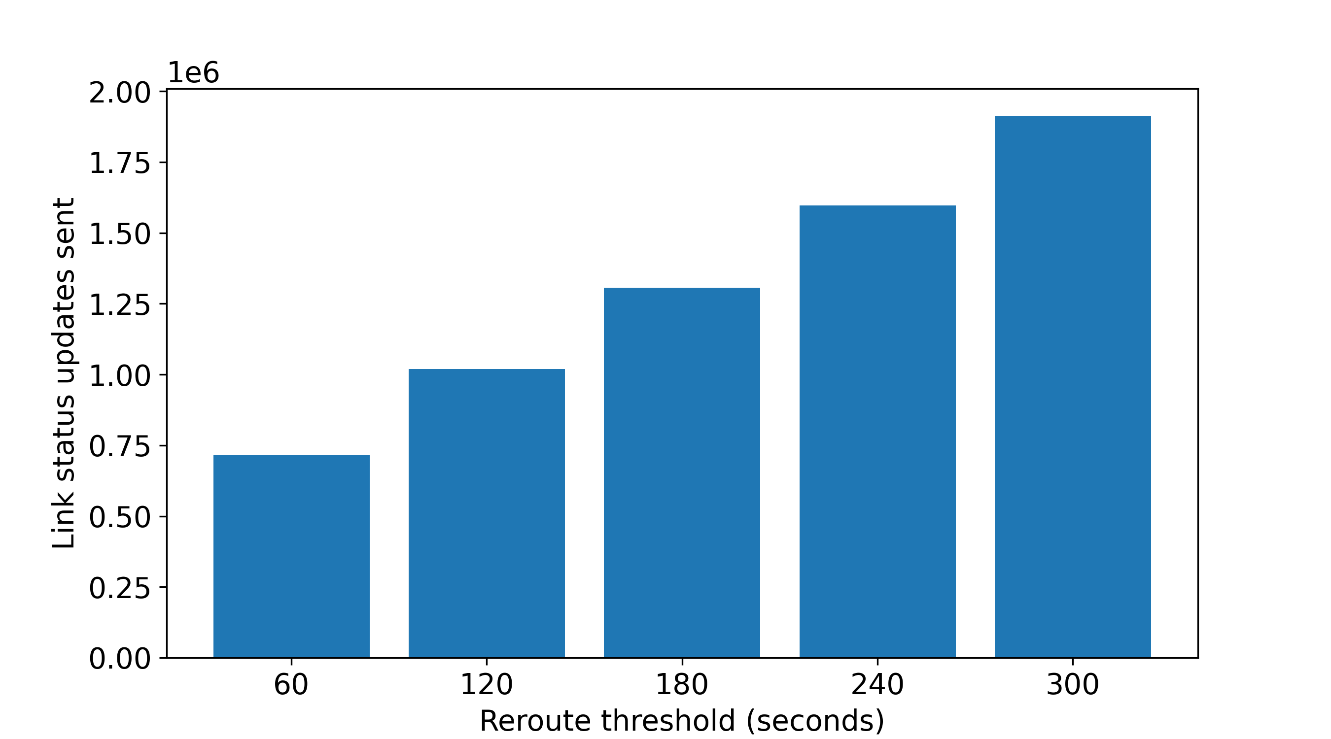
(a) Link Status Updates Sent

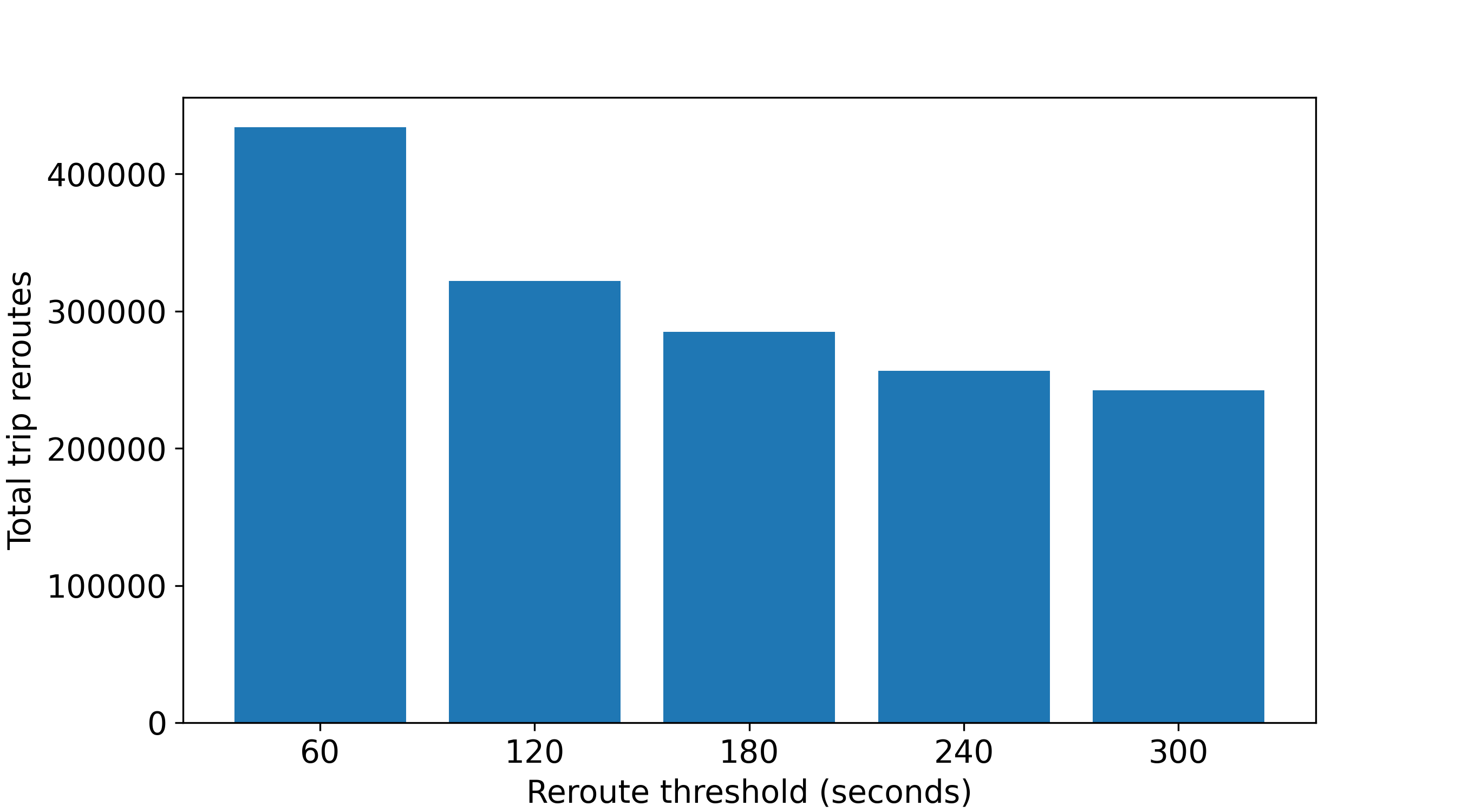
(b) Trip Leg Reroutes

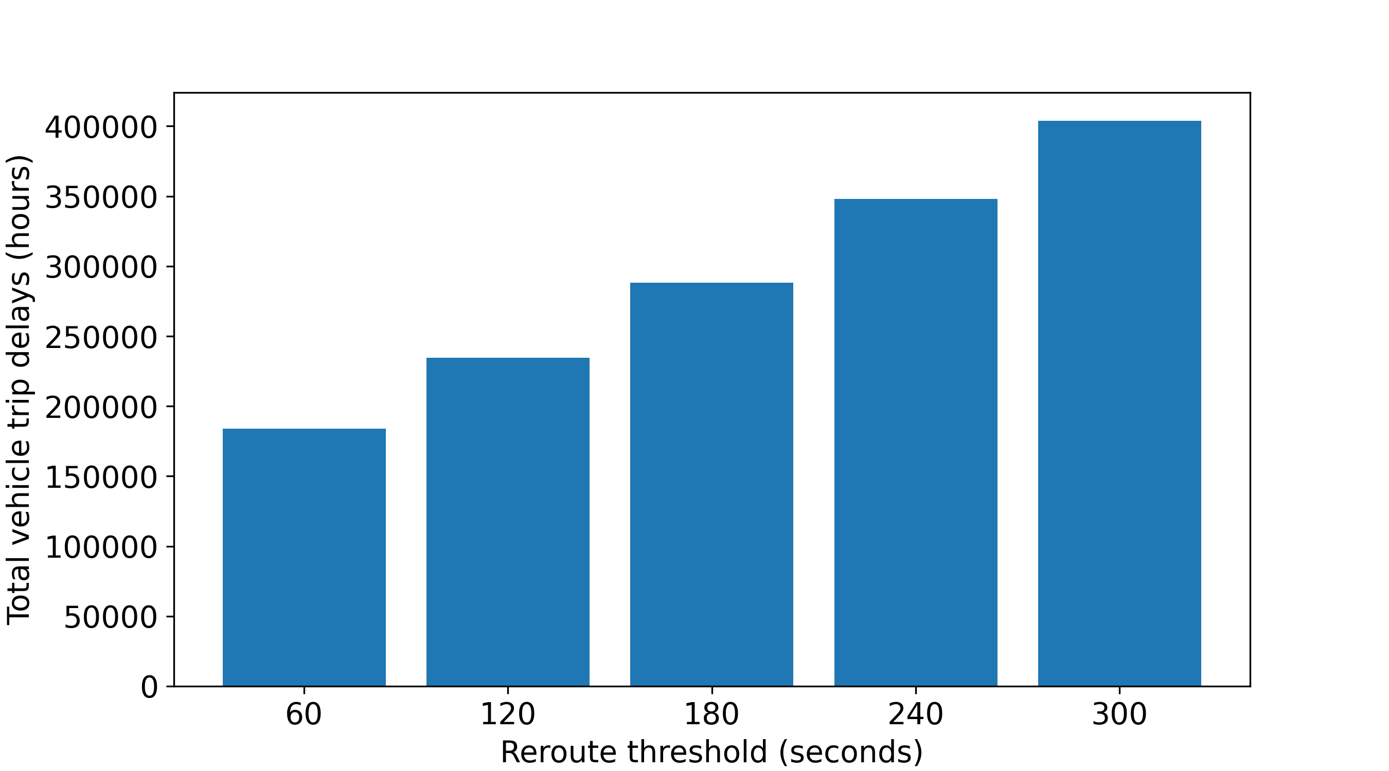
(c) Total (System) Vehicle Delay

Figure 13. Parameter sensitivity sweep for rerouting delay and difference thresholds. X-axis is the absolute reroute delay threshold $t_{\text{delay}}$, where $r_{\text{delay}}=t_{\text{delay}}/600$.

For the experiments in the next section, we used the parameter values in Table 1, which provide a good balance between realism and improvement in system congestion. The parameters with the largest effect on total system delay were the reroute threshold parameters ($t_{\text{delay}}$ and $r_{\text{delay}}$). For these, we selected $t_{\text{delay}}$ equal to 2 minutes and $r_{\text{delay}}$ equal to 0.2 as a compromise between system efficiency and excessive rerouting.

4. EXPERIMENTS

4.1. Experimental Methodology Description

In order to demonstrate and evaluate our Mobiliti simulator, we followed the following steps to model and analyze road network traffic in the San Francisco Bay Area (the steps would be similar for other areas). First, we obtained the necessary network, trip demand, and vehicle data inputs shown in Figure 2, left. After obtaining the inputs, we run the Mobiliti simulator (Figure 2, center) for a variety of parameter configurations, including sweeping the dynamic rerouting penetration rate, the link status update threshold, the reroute check interval, and the reroute threshold. The simulator outputs include link-level metrics such as vehicle counts, average speeds, and congestion delay series; leg-level metrics such as trip times and delays; and rerouting information such as when and where rerouting occurs. We then process the simulator logs and outputs (Figure 2, right) using a combination of software tools (such as Python) to conduct the various analyses presented in the following subsections.

The road network model was derived from a HERE Technologies (HERE Technologies, 2019) map consisting of 454,651 nodes and 1,008,959 links spanning from Santa Rosa, Napa, and Vacaville to the north, San Jose to the south, and Oakland, Hayward, Fremont, and Livermore to the east (see Figure 8). While the link actor model currently supports the signal timing mechanism described in Section 3.1, the following experiments were run without detailed signal behavior due to lack of comprehensive, accurate location and timing data for all of the signals in the Bay Area. However, the link capacity properties in the input road network already take into account the presence of signals and are used in each link actor’s Congestion Delay Model (see Section 3.1) to compute vehicle traversal times, thus the simulator slows vehicles according to those flow capacity values compared to having no signals.

The trip demand is initialized from an input file with 19 million trip legs (origin/destination pairs) based on disaggregate simulated trip records from the San Francisco County Transportation Authority (SFCTA) SF CHAMP 6.1 model (SFCTA, 2019). Each trip leg is specified with origin and destination travel analysis zones (chosen from 40,000 micro-analysis zones) and a start time. Since our simulator models each individual vehicle traversing from link to link at discrete times, we chose specific origin and destination nodes within the given TAZs. We weighted each node by its nearby population density derived from the Global Human Settlement database (European Commission, Joint Research Centre ; Columbia University, Center for International Earth Science Information Network - CIESIN(2015), JRC) to avoid choosing nodes that are in very sparsely populated regions of the map, which would unrealistically send traffic to remote areas. We also avoided selecting freeway or ramp nodes as origins or destinations. Figure 14 shows the population density map we used for initializing our simulated trip legs. Note that the coarse granularity of the heat map is a result of the resolution of the provided data set (250 meters).

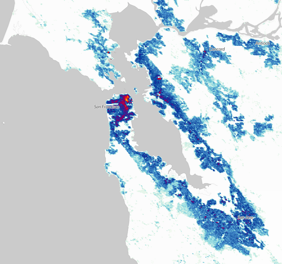
Figure 14. GHS density map (European Commission, Joint Research Centre ; Columbia University, Center for International Earth Science Information Network - CIESIN(2015), JRC) showing where people live as a function of geographical location. Mobiliti uses this information coupled with a TAZ-to-TAZ demand model to compute specific node origins and node destinations for each trip leg. The raster resolution of the GHS data is 250 meters by 250 meters. Red shows high population density, followed by dark blue with medium density and lighter blues with low density.

Figure 15a shows the temporal profile of the SFCTA demand model’s trip legs during the simulated model day. Our simulation runs a single model day, and the figure shows on the y-axis the number of trips that start in each hour of the day. The number of trip legs per hour varies from very low in the early morning hours to very high during late afternoon rush hour. Since trip lengths can vary considerably, by weighing each trip by its length, Figure 15b shows the VMT (total trip distance) by start time, which is defined as the sum of the total trip distance over all trips that start in each hour of the day. This figure illustrates the time-varying magnitude of the total load on the road network.

(a) (a) Total trip legs by start time

(b) (b) VMT (total trip distance) by start time

Figure 15. These figures give a temporal profile of how demand evolves through the simulated day. Figure (a) shows the total number of trip legs starting at different times of the day. Figure (b) shows the VMT (total trip distance) summed over trips that start at different times of day.

4.2. Computational Performance

This section details the design and analysis of the computational performance of the Mobiliti simulator. For our experiments, we ran Mobiliti on the Cori supercomputer (NERSC, 2018). Adding dynamic rerouting adds significant computational cost to the simulation compared to the original statically routed case. This is mainly due to the addition of shortest path route calculations by VehicleController actors during RerouteCheck events, and also due to the additional processing of LinkStatusUpdate events. Not only does the cost of calculating new routes directly add to the simulation time, but the irregularity of congestion also causes load imbalance of compute workload across the simulator’s parallel compute cores. We mitigate this effect by using an efficient routing algorithm (Customizable Contraction Hierarchies (Geisberger et al., 2012; Dibbelt et al., 2014)) via the RoutingKit (RoutingKit, 2019) library. RoutingKit’s Customizable Contraction Hierarchies library employs relatively costly preprocessing steps (i.e. partial customizations) to enable very efficient subsequent routing queries. This strategy is ideal for computing many routes in a network with static weights, since the cost of the preprocessing step can be amortized across all of the subsequent queries.

However, in a dynamic rerouting simulation the link weights are constantly changing due to congestion varying over the course of the simulated day. In order to support dynamically changing link weights, we designed the VehicleController to keep track of which links have updated their travel time since the previous customization, and then only re-customize the contraction hierarchy when a RerouteCheck query is received. This method of batching LinkStatusUpdates avoids excessive re-customizations every time an update is received. Furthermore, if no congestion update is received during a sequence of RerouteCheck queries, they can all use the same customization and thus be serviced very efficiently.

Figure 16(a) shows the parallel scaling performance of Mobiliti when simulating a full normal model day with 19 million trip legs over the San Francisco Bay 0.5 million nodes and 1 million links with 50 percent dynamic rerouting penetration. The dashed line represents theoretical perfect linear scaling performance. As we increase the core count from 1 to 512, the simulation execution time (excluding program initialization) is reduced from more than six hours to less than three minutes, corresponding to a 130x speed up versus serial execution.

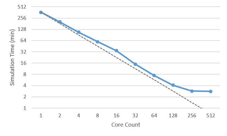
(a)

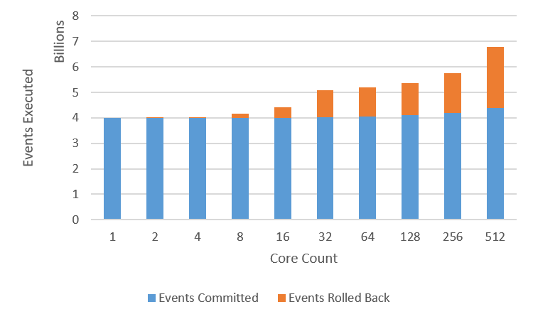
(b)

Figure 16. (a) Mobiliti simulation times (excluding program initialization) as we vary the core count from 1 to 512 cores of the Cori-Haswell computer at NERSC (NERSC, 2018). All times shown are for simulating 19 million trip legs with 50 percent dynamic rerouting penetration on the whole San Francisco Bay Area road network with 0.5 million nodes and 1 million links. When simulating a normal model day, execution time is decreased from over six hours on one core to less than three minutes on 512 cores running in parallel. (b) Mobiliti total events executed as the core count is varied from 1 to 512 cores. Executed events are either committed (successful) or rolled back (unsuccessful).

For the shared memory runs (16 cores or fewer), we use a single process, multi-threaded configuration (utilizing one thread per core). Using shared memory avoids the overheads of inter-process communication, but limits execution to a single node. For the distributed memory runs (32 cores or more), we use a multi-process, multi-threaded configuration with hyper-threading (two threads per core), which enables executing on multiple nodes, better data locality in the memory subsystem due to non-uniform memory access (Majo and Gross, 2011), and higher core utilization. Furthermore, strong scaling (increasing core count for a fixed problem size) yields the benefit of reducing the active working set size for each core, enabling better data re-use and on-chip cache utilization. Figure 16(b) shows the total number of events committed and rolled back for each of the runs in the scaling study. For the single core run, there is no misspeculation because events are trivially executed in increasing timestamp order. As the number of cores increases, commit efficiency (events committed / total events executed) levels off around 90 percent for the shared memory runs and ranges from 79 to 65 percent for distributed memory runs.

We note that performance improvements from increasing parallelism level off at 512 cores and suspect the scalability could be further improved for even higher core counts by tuning the parallel distribution of the dynamic re-routing workload to refine the computational load balance and reduce mis-speculation overhead in the simulator. A more in-depth parallel performance study of the simulator will be explored in future work.

4.3. Impact of dynamic rerouting on system metrics

To understand the effect of rerouting penetration, we enabled dynamic rerouting for varying percentages of vehicle trip legs for the entire Bay Area. We chose to study a range of penetration rates from 0% to 100% at 10% increments. Figure 17 illustrates the impact of enabling dynamic rerouting for 100% vehicle trips for the entire metropolitan-scale system simulated. The difference between baseline and 100% rerouting case is that the former uses static shortest path routes based on free speed traversal times, whereas the latter uses dynamic routes computed by the vehicle controllers based on their knowledge of the current traffic congestion patterns. In Figure 17, blue links handle a lesser number of vehicle traversals when 100% dynamic rerouting is enabled, while the red links handle a greater number. The figure shows how the traffic is rerouted away from certain links to reduce congestion (blue), while other links end up handling higher traffic (red).

(a) (a) Bay Area

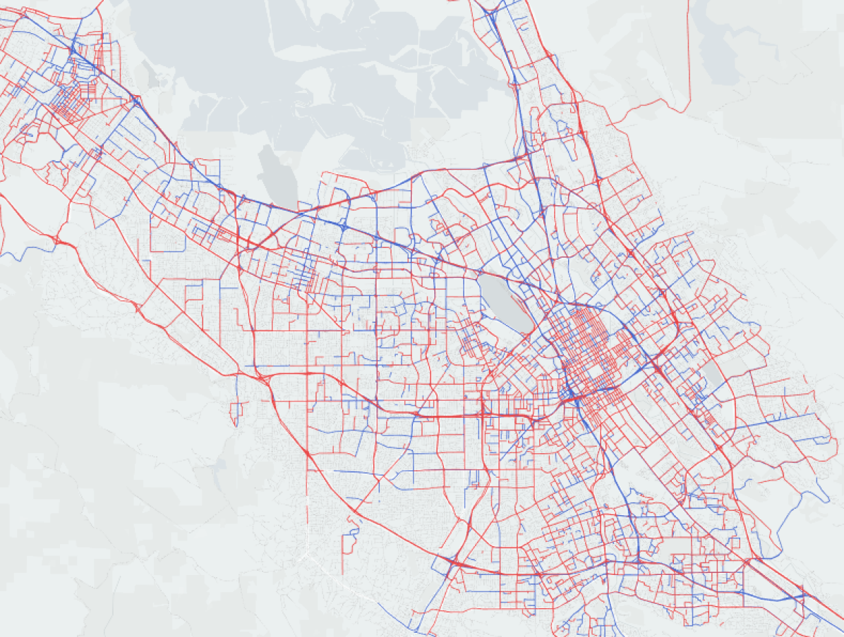
(b) (b) San Jose Region

Figure 17. System-wide impact on number of vehicle link traversals from enabling dynamic rerouting (Baseline versus 100% penetration). Red or blue represent a increase or decrease in vehicle traversal count respectively for a day.

Figure  18 shows how the reroutes are temporally distributed throughout the simulation day, illustrating that almost 80% of the rerouting occurs during the morning and evening rush hours when the demand is the highest. The distribution of reroutes is heavily influenced by the temporal distribution of trip legs in the demand model input (Figure 15). As can be seen in Figure 15b, there is a peak in the VMT in the morning (7am to 10 am) and the evening rush hours (3:30 pm to 6:30 pm). Because the level of demand during the rush hours is the highest, we see corresponding peaks in the number of reroutes. Further, it needs to be noted that penetration rate indicates the number of trip legs that are allowed to reroute, but not all reroutable trip legs do actually reroute. Table 2 indicates the percentage of trip legs that actually got rerouted as a percentage of allowed reroutable legs. It can be seen that at higher penetration rates the percentage decreases even though the actual number of reroutes is higher, as not many trip legs engage in any relevant congestion and hence do not reroute. Furthermore, among the trips that do reroute, the number of reroutes per trip remains small, with 99.9% of trips rerouting three times or fewer in the 100% penetration scenario.

Figure 18. The figure give a temporal profile of the rate of dynamic vehicle reroutes for a day. Sharp increases in number of reroutes can be seen in the morning and evening peak hours.

Table 2. Share of Rerouted Trip Legs

Penetration rate	Trip legs reroutable	Trip legs rerouted	Percentage rerouted
(%)	(in thousands)	(in thousands)	(%)
10	1,900	130	7
20	3,800	221	6
30	5,700	274	5
40	7,600	291	4
50	9,500	301	3
60	11,400	317	3
70	13,300	329	2
80	15,200	340	2
90	17,100	355	2
100	19,000	374	2

Using the delay and fuel model described in our previous work (Chan et al., 2018), we are able to make impact estimates for dynamic rerouting penetration rates. Figure 19 exhibits the system level vehicle hours of delay (VHD) and number of reroutes for different penetration levels and Table 3 shows the system level vehicle miles travelled (VMT) and fuel consumption resulting from the dynamic rerouting. As the penetration rate increases, the delay reduces without any significant change in VMT. The minimum system delay is obtained with 100% penetration rate. However, if we look at the “knee of the curve” for VHD, the return starts diminishing after 70% penetration. On average, a rerouted trip saves 16 minutes in travel time with no additional trip distance with 100% penetration rate compared to baseline as shown in Figure 20(a).

Figure 19. System wide vehicle hours of delay (VHD) and the number of trip legs rerouted from varying the dynamic rerouting penetration rates. As the penetration rate increases, the overall system delay reduces. If we look at the elbow of the VHD curve, after 70% penetration rate the returns start diminishing.

Table 3. VMT and Fuel Consumption

Penetration rate	VMT	Fuel
	(in thousand miles)	(in thousand gallons)
0%	146,847	5,906
10%	146,783	5,903
20%	146,707	5,899
30%	146,652	5,894
40%	146,605	5,891
50%	146,572	5,888
60%	146,546	5,886
70%	146,537	5,884
80%	146,517	5,883
90%	146,505	5,882
100%	146,490	5,882

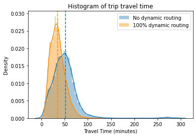
(a) Distribution of the travel times for trip legs. The mean travel time per trip leg with 100% dynamic routing is 35 minutes and without is 51 minutes as showed by the corresponding orange and blue vertical lines.

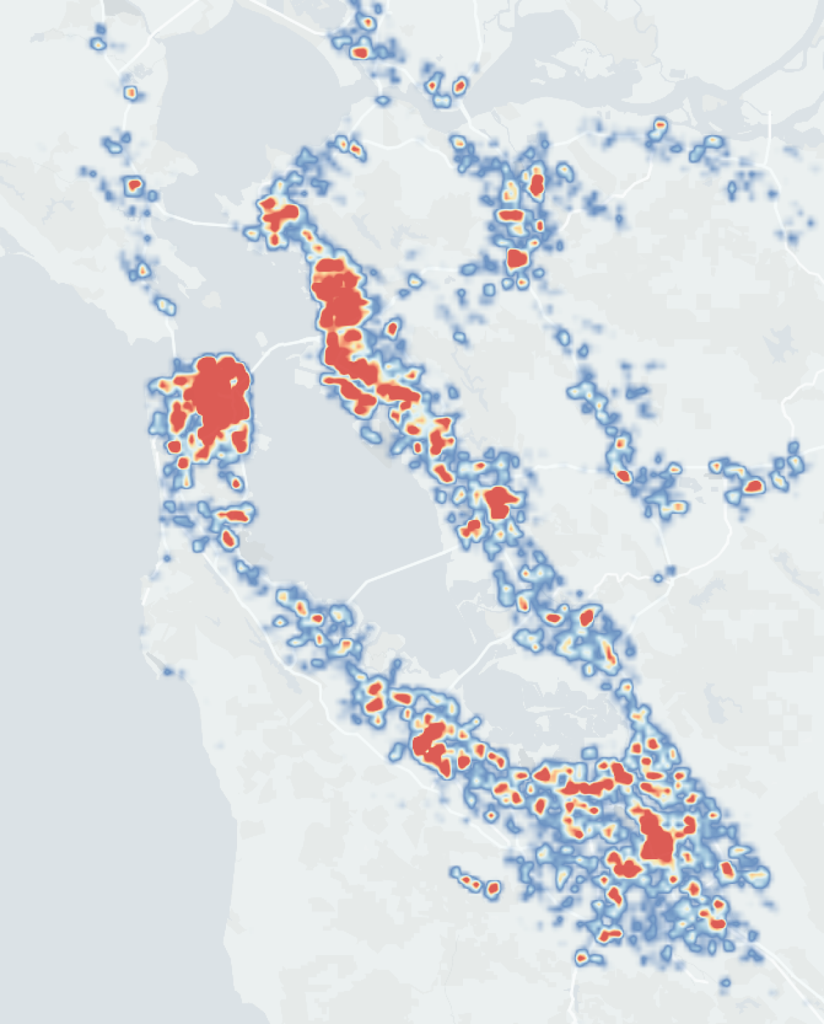
(b) Heat map of areas with highest congestion (v/c over 0.75) with increased vehicle counts due to dynamic rerouting in the morning rush hour for functional class 5 links. Red indicates high congestion and blue represents low congestion.

Figure 20.

We observe that dynamic rerouting effectively rearranges the vehicle flows from high utilization highways and arterials to low utilization neighborhood links to reduce the overall system delay. We analyze these effects by investigating the rearrangement of traffic flow by functional classification of links. We maintain the definitions of functional class roads as defined by HERE Technologies (HERE Technologies, 2019). Specifically, functional classes are hierarchical classification of roads according to the speed, importance and connectivity of the road. A road can be one of five functional classes defined in Table 4.

Table 4. Functional Road Classes

Functional class	Definition
1	Allows high volume, maximum speed traffic movement
2	Allows high volume, high speed traffic movement
3	Provides high volume of traffic movement
4	Provides high volume of traffic movement at moderate speeds between neighborhoods
5	Local roads with volume and traffic movement below the level of any functional class

By examining the traffic flow by functional classes with 100% dynamic rerouting penetration, we observe that traffic shifts from FC 2 and 3 to FC 4 and 5. This reduces the delay on highways significantly while increasing traffic on FC 5 in the morning and evening peaks. It is also interesting to note that the increase in traffic volume on FC 5 does not always cause congestion in those links as many links do not reach congested levels with the increased flow. Specifically, 7000 kilometers of FC 5 links received additional traffic flow with 100% dynamic rerouting, of which 75% received fewer than 6 additional vehicles during the morning peak.

Of the FC 5 links with increased traffic volume, 440 kilometers are congested with a volume over capacity ratio higher than 0.75. Spatial analysis of the congestion shows the cities of San Francisco, San Jose, Berkeley, Oakland and Fremont are the most affected by the increased traffic in the local roads (Figure  20(b)). The local roads (FC 5) in these cities has a mean increase of 70 vehicles during the morning peak. Finally, of the 440 kilometers of congested road network in the morning peak, 110 kilometers reflects new congestion created due to dynamic rerouting on the local roads. These roads would arguably be some of the most negatively impacted areas by high dynamic rerouting penetrations.

Finally, we present the results of user equilibrium traffic assignment (UE) in Table 5 for comparison using the methods we describe in (Chan et al., 2021). Comparing with the system metrics for dynamic rerouting with 100% penetration rate, we can see that VHD is nearly half, fuel consumption is slightly higher and VMT slightly lower in user equilibrium. Since the user equilibrium is a steady-state solution computed through iterative optimization, it results in routes with lower delays than the more reactive dynamic rerouting approach. However, in reality, the user equilibrium state in never actually achieved and hence congestion is underestimated in the user equilibrium case.

Table 5. User Equilibrium System Metrics

	VMT	VHD	Fuel
	(in thousand miles)	(in thousand hours)	(in thousand gallons)
User Equilibrium	146,051	90	5,915

4.4. Validation

Validation was performed for the simulation runs with different penetration rates to test the effectiveness of representing the real world traffic environment. We conducted a three stage validation procedure using multiple data sources. Our results show that the simulation with 60% dynamic rerouting is the closest to representing the real world traffic. For brevity, we have only included the validation for this penetration rate here. Our results are also consistent with multiple surveys stating that the percentage of Americans having smartphones who uses online maps or navigation services daily ranges from 55% to 65% (Statista, 2021; EMarketer, 2021; Manifest, 2021).

Stage 1 of the validation procedure involves comparing the traffic flows or counts between the simulation and real world. This includes checking a) traffic counts for eight corridor links in San Jose city, b) average daily traffic counts (ADT) for four main bridges in the Bay Area, and c) traffic flows for all major highways in the Bay area. The traffic count for each link was compared against the field data for the entire day in 15 minutes increments. The field data for city roads and highways were collected from the city of San Jose and Caltrans PeMS website (DOT, 2021) respectively for the year 2019. Each corridor provided information regarding traffic volumes by time of the day and direction. For PeMS data, since it is prone to measurement error, data from multiple weekdays in April and May 2019 were averaged to get a typical day value. A coefficient of determination (R²) of 0.7 which is typically used as a satisfactory criterion for link count checks is used as the threshold. The Figure 21 shows R² values for the eight corridors under consideration. The modeled corridors indicate a close match with the field data with the lowest R² value observed being 0.76 for Zanker road.

Figure 21. Validation of traffic counts in 15 minute increments for links in different functional classes. All links have satisfactory R² of greater than 0.7.

Additionally, ADT for four main bridges in the Bay Area in both directions is shown in Table 6. The field data was obtained from the Caltrans website (DOT, 2021) for the year 2019. The target error was $\pm 25\%$, and seven out of the eight links met this criterion. We believe that the high relative error for the Golden Gate Bridge NB count is due to the Caltrans field count not being an accurate representation of the actual bridge count. The discrepancy is due to the sensor placement after a major exit, which results in a significant percentage of bridge traffic not being counted by the sensor.

Table 6. ADT Check

Sl No	Bridge	Field Count	Simulation Count	Relative Error (%)
1	I-580 Richmond San Rafael Bridge EB	56182	51551	-8%
2	I-580 Richmond San Rafael Bridge WB	41597	52131	25%
3	I-80 Bay Bridge EB	132000	148105	12%
4	I-80 Bay Bridge WB	131861	139993	6%
5	US-101 Golden Gate Bridge NB	32212∗	63730	98%
6	US-101 Golden Gate Bridge SB	74526	70020	-6%
7	CA-92 San Mateo Bridge EB	56510	53684	-5%
8	CA-92 San Mateo Bridge WB	62597	50199	-20%

*Golden Gate Bridge NB link’s closest PeMS sensor is located after an off ramp and hence the field count does not reflect the full bridge traffic count.

Next, we evaluated R² for all links that have a corresponding PeMS sensor in Bay Area. We were able to match 2061 links with mainline sensors and the resulting R² distribution is shown in Figure  22a. Of the total matched links, 72% links have R² greater than 0.7 and 5% have lower than 0.4 (Figure  22b).

(a) Distribution of R² values for the highway links. It follows a left skewed normal distribution with mean 0.75 and standard deviation 0.15

(b) Spatial distribution of R² values of the links.

Figure 22. Evaluation metrics for highway link flows compared to PeMS sensors.

Stage 2 in the validation procedure is speed comparison with a) Uber Movement data for San Francisco city streets, and b) PeMS speed data for Bay Area highways. For Uber Movement, speed data for San Francisco region for Q4, 2019 (Uber, 2021) is used for comparison. Links from Uber’s network were matched to Mobiliti links for a total of 139,495 links (20% of total) in the simulation. The speeds were compared for 8 am to 9 am for different speed limits. Figure 23 shows the average speeds from Mobiliti and Uber across all speed limits and Figure 24 shows the speed distributions from Mobiliti and Uber on links with 60 mph and 70 mph speed limit.

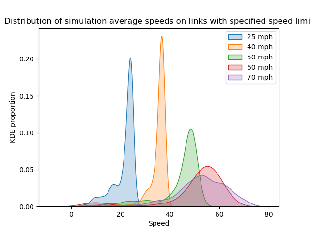
Figure 23. Average Uber (left) and Mobiliti (right) speeds across all speed limits 8am to 9am in the morning.

Figure 24. Kernel density comparing Mobiliti and Uber speed distributions at 60 mph (left) and 70 mph (right).

Next we compared highway links with PeMS speed profiles for the 2061 matched links. Figure 25 shows the difference in speeds between simulation and PeMS at 9 am and 3pm for a weekday. Most links are within $\pm 20$ mph difference. Further, R² values were evaluated for all links to understand the time series trends. Figure 26 shows a time series comparison for six highway links. Of the total, 55% of highway links have R² greater than 0.4. We plan to improve the speed models to reflect time series trends closer to real world data in the future.

Figure 25. Figure shows the histogram of speed difference between simulation and PeMS at 9am and 3pm for highways in Bay Area.

Figure 26. Simulation and PeMS speed profile for highways. Yellow line represents the average weekday values from PeMS. The first and second standard deviation bands are shown around the average. Green line represents the simulation speed for a typical day.

Stage 3 is system level comparisons, network validation, and error checking. Model visualization is used to check for unusual activities in traffic flows and odd roadway network attributes. Error checking and model verification consist of several smaller tasks such as checks for link geometry and connectivity, link speeds, and ramp and intersection geometry. Since our travel demand data was obtained from SFCTA, which conducts their own validation, we did not conduct additional behavior checks. We conducted system metric checks for VMT and total demand and validated them against the 2017 Environmental Impact report for the Bay Area (EIRPBA, 2021) in Table 7.

Table 7. System level metrics

Metric	Simulation	Field Data	Relative Error(%)
VMT	146,546,360	158,406,800	-7
Daily Trips	19,167,301	21,227,800	-10

5. Conclusion

Vehicles are rapidly gaining the ability to utilize up-to-date road congestion information to re-route their paths during their trips through smartphone navigation apps. In this paper, we presented a computational methodology to model varying degrees of dynamic rerouting in a large-scale transportation system using the Mobiliti high-performance parallel discrete event simulator. We described updates to our link actor model to capture the effects of link congestion, timing constraints, and storage capacity constraints. We have detailed the implementation of new VehicleController actors and the events required to update their knowledge of the system state and service dynamic rerouting requests. Because we have designed our simulator to scale over distributed memory parallel computing platforms, we can simulate one model day of the San Franscisco Bay Area with 19 million vehicle trips and 50 percent dynamic rerouting penetration over a road network with 0.5 million nodes and 1 million links in three minutes of simulation time. We conducted an analysis of system-level impacts when varying the dynamic rerouting penetration rate at 10% increments and examined the varying effects on different functional classes and geographical regions. Finally, we presented a validation of the simulation results compared to real world data sources.

- (1)
- Abrams (1989) M. Abrams. 1989. a common programming structure for Bryant-Chandy-Misra, time-warp, and sequential simulators. In Proceedings of the 21st conference on Winter simulation (WSC ’89). Association for Computing Machinery, New York, NY, USA, 661–670. https://doi.org/10.1145/76738.76823
- Auld et al. (2016) Joshua Auld, Michael Hope, Hubert Ley, Vadim Sokolov, Bo Xu, and Kuilin Zhang. 2016. POLARIS: Agent-based modeling framework development and implementation for integrated travel demand and network and operations simulations. Transportation Research Part C: Emerging Technologies 64 (2016), 101–116.
- Auld et al. (2019) Joshua Auld, Omer Verbas, and Monique Stinson. 2019. Agent-based dynamic traffic assignment with information mixing. Procedia Computer Science 151 (2019), 864–869.
- Barnes et al. (2013) Peter D. Barnes, Jr., Christopher D. Carothers, David R. Jefferson, and Justin M. LaPre. 2013. Warp Speed: Executing Time Warp on 1,966,080 Cores. In Conference on Principles of Advanced Discrete Simulation (Montr©al, Québec, Canada). 327–336. https://doi.org/10.1145/2486092.2486134
- Bauer Jr. et al. (2009) David W. Bauer Jr., Christopher D. Carothers, and Akintayo Holder. 2009. Scalable Time Warp on Blue Gene Supercomputers. In Workshop on Principles of Advanced and Distributed Simulation. 35–44. https://doi.org/10.1109/PADS.2009.21
- Behrisch et al. (2008) Michael Behrisch, Daniel Krajzewicz, and Yun-Pang Wang. 2008. Comparing performance and quality of traffic assignment techniques for microscopic road traffic simulations. Proceedings of DTA2008 (2008).
- Ben-Akiva et al. (2002) Moshe Ben-Akiva, Michel Bierlaire, Haris N Koutsopoulos, and Rabi Mishalani. 2002. Real time simulation of traffic demand-supply interactions within DynaMIT. In Transportation and network analysis: current trends. Springer, 19–36.
- CAL (2017) CAL. 2017. California fires: navigation apps like Waze sent commuters into flames, drivers say. https://www.usatoday.com/story/tech/news/2017/12/07/california-fires-navigation-apps-like-waze-sent-commuters-into-flames-drivers/930904001/
- Casas et al. (2010) Jordi Casas, Jaime L. Ferrer, David Garcia, Josep Perarnau, and Alex Torday. 2010. Traffic Simulation with Aimsun. Springer New York, New York, NY, 173–232.
- Chan et al. (2018) Cy Chan, Bin Wang, John Bachan, and Jane Macfarlane. 2018. Mobiliti: Scalable Transportation Simulation Using High-Performance Parallel Computing. In 2018 21st International Conference on Intelligent Transportation Systems (ITSC). IEEE, Maui, HI, 634–641. https://doi.org/10.1109/ITSC.2018.8569397
- Chan et al. (2021) Cy P. Chan, Anu Kuncheria, Bingyu Zhao, Theophile Cabannes, Alexander Keimer, Bin Wang, Alexandre M. Bayen, and Jane MacFarlane. 2021. Quasi-Dynamic Traffic Assignment using High Performance Computing. CoRR abs/2104.12911 (2021). arXiv:2104.12911 https://arxiv.org/abs/2104.12911
- Chandy and Misra (1979) K.M. Chandy and J. Misra. 1979. Distributed Simulation: A Case Study in Design and Verification of Distributed Programs. IEEE Transactions on Software Engineering SE-5, 5 (Sept. 1979), 440–452. https://doi.org/10.1109/TSE.1979.230182 Conference Name: IEEE Transactions on Software Engineering.
- Dibbelt et al. (2014) Julian Dibbelt, Ben Strasser, and Dorothea Wagner. 2014. Customizable Contraction Hierarchies. In Experimental Algorithms, Joachim Gudmundsson and Jyrki Katajainen (Eds.). Springer International Publishing, Cham, 271–282.
- DOT (2021) CA DOT. 2021. Traffic Volumes | Caltrans. https://dot.ca.gov/programs/traffic-operations/census/traffic-volumes
- EIRPBA (2021) EIRPBA. 2021. Environmental Impact Report Plan Bay Area. https://www.planbayarea.org/2040-plan/environmental-impact-report
- EMarketer (2021) EMarketer. 2021. Maps and Navigation Apps Are Still Essential to Smartphone Experience, and User Penetration Continues to Grow. https://www.emarketer.com/content/people-continue-to-rely-on-maps-and-navigational-apps-emarketer-forecasts-show
- European Commission, Joint Research Centre ; Columbia University, Center for International Earth Science Information Network - CIESIN(2015) (JRC) European Commission, Joint Research Centre (JRC); Columbia University, Center for International Earth Science Information Network - CIESIN. 2015. GHS population grid, derived from GPW4, multitemporal (2015). http://data.europa.eu/89h/jrc-ghsl-ghs_pop_gpw4_globe_r2015a. European Commission, Joint Research Centre (JRC) [Dataset].
- FHWA (2021) FHWA. 2021. Traffic Analysis Toolbox Volume XIV: Guidebook on the Utilization of Dynamic Traffic Assignment in Modeling - Section 2. https://ops.fhwa.dot.gov/publications/fhwahop13015/sec2.htm
- Fujimoto (1990) Richard M. Fujimoto. 1990. Parallel discrete event simulation. Commun. ACM 33, 10 (Oct. 1990), 30–53. https://doi.org/10.1145/84537.84545
- Geisberger et al. (2012) Robert Geisberger, Peter Sanders, Dominik Schultes, and Christian Vetter. 2012. Exact Routing in Large Road Networks Using Contraction Hierarchies. Transportation Science 46, 3 (Aug. 2012), 388–404. https://doi.org/10.1287/trsc.1110.0401
- HERE Technologies (2019) HERE Technologies. 2019. https://www.here.com/. [Online; accessed 06-Feb-2019].
- Jefferson (1985) David R. Jefferson. 1985. Virtual Time. ACM Trans. Program. Lang. Syst. 7, 3 (July 1985), 404–425. https://doi.org/10.1145/3916.3988
- Kim et al. (2009) Hyunmyung Kim, Jun-Seok Oh, and R Jayakrishnan. 2009. Effects of user equilibrium assumptions on network traffic pattern. KSCE Journal of Civil Engineering 13, 2 (2009), 117–127.
- Kim et al. (2020) Kyungtae Kim, Seokjoo Koo, and Ji-Woong Choi. 2020. Analysis on Path Rerouting Algorithm based on V2X Communication for Traffic Flow Improvement. In 2020 International Conference on Information and Communication Technology Convergence (ICTC). IEEE, 251–254.
- Kucharski and Gentile (2019) Rafał Kucharski and Guido Gentile. 2019. Simulation of rerouting phenomena in dynamic traffic assignment with the information comply model. Transportation Research Part B: Methodological 126 (2019), 414–441.
- Liang and Wakahara (2014) Zilu Liang and Yasushi Wakahara. 2014. Real-time urban traffic amount prediction models for dynamic route guidance systems. EURASIP Journal on Wireless Communications and Networking 2014, 1 (May 2014), 85. https://doi.org/10.1186/1687-1499-2014-85
- Lopez et al. (2018) Pablo Alvarez Lopez, Michael Behrisch, Laura Bieker-Walz, Jakob Erdmann, Yun-Pang Flötteröd, Robert Hilbrich, Leonhard Lücken, Johannes Rummel, Peter Wagner, and Evamarie Wießner. 2018. Microscopic traffic simulation using sumo. In 2018 21st international conference on intelligent transportation systems (ITSC). IEEE, 2575–2582.
- Mahmassani (1998) Hani Mahmassani. 1998. Dynamic Traffic Simulation and Assignment: Models, Algorithms and Application to ATIS / ATMS Evaluation and Operation. 104–135. https://doi.org/10.1007/978-3-662-03514-6_5
- Majo and Gross (2011) Zoltan Majo and Thomas R Gross. 2011. Memory system performance in a NUMA multicore multiprocessor. In Proceedings of the 4th Annual International Conference on Systems and Storage. 1–10.
- Manifest (2021) The Manifest. 2021. The Popularity of Google Maps: Trends in Navigation Apps in 2018 | The Manifest. https://themanifest.com/mobile-apps/popularity-google-maps-trends-navigation-apps-2018
- MATSIM (2020) MATSIM. 2020. MATSim.org. https://www.matsim.org/
- NERSC (2018) NERSC. 2018. Cori Configuration. http://www.nersc.gov/users/computational-systems/cori/configuration/. [Online; accessed 27-Apr-2018].
- Perumalla (2006) Kalyan S. Perumalla. 2006. A Systems Approach to Scalable Transportation Network Modeling. In Proceedings of the 2006 Winter Simulation Conference. 1500–1507. https://doi.org/10.1109/WSC.2006.322919 ISSN: 1558-4305.
- Qurashi et al. (2020) Moeid Qurashi, Hai Jiang, and Constantinos Antoniou. 2020. Modeling autonomous dynamic vanpooling services in sumo by integrating the dynamic routing scheduler. In SUMO User Conference.
- Rakha et al. (2012) Hesham A. Rakha, Kyoungho Ahn, and Kevin Moran. 2012. INTEGRATION Framework for Modeling Eco-routing Strategies: Logic and Preliminary Results. International Journal of Transportation Science and Technology 1, 3 (Sept. 2012), 259–274. https://doi.org/10.1260/2046-0430.1.3.259
- Rojo (2020) Marta Rojo. 2020. Evaluation of traffic assignment models through simulation. Sustainability 12, 14 (2020), 5536.
- RoutingKit (2019) RoutingKit. 2019. https://github.com/RoutingKit/RoutingKit. [Online; accessed 28-Jan-2019].
- SFCTA (2019) SFCTA. 2019. SF-CHAMP 6.1: ConnectSF Needs Assessment 2015 Base Year Model Run. Technical Report. San Francisco County Transportation Authority.
- Sheppard et al. (2017) Colin Sheppard, Rashid Waraich, Andrew Campbell, Alexei Pozdnukov, and Anand R. Gopal. 2017. Modeling plug-in electric vehicle charging demand with BEAM: the framework for behavior energy autonomy mobility. Technical Report 1398472. 1398472 pages. https://doi.org/10.2172/1398472
- Statista (2021) Statista. 2021. People who use their cell phone for maps/GPS navigation in the U.S. 2018, by age. https://www.statista.com/statistics/231615/people-who-use-their-cell-phone-for-maps-gps-navigation-usa/
- Thulasidasan and Eidenbenz (2009) Sunil Thulasidasan and Stephan Eidenbenz. 2009. Accelerating traffic microsimulations: A parallel discrete-event queue-based approach for speed and scale. In Proceedings of the 2009 Winter Simulation Conference (WSC). IEEE, 2457–2466.
- Tseng and Ferng (2021) Ying-TSU Tseng and Huei-Wen Ferng. 2021. An Improved Traffic Rerouting Strategy Using Real-Time Traffic Information and Decisive Weights. IEEE Transactions on Vehicular Technology (2021).
- Uber (2021) Uber. 2021. Uber Movement: Let’s find smarter ways forward, together. https://movement.uber.com/cities/san_francisco/downloads/speeds
- Ugirumurera et al. (2018) Juliette Ugirumurera, Gabriel Gomes, Emily Porter, Xiaoye S. Li, and Alexandre Bayen. 2018. A unified software framework for solving traffic assignment problems. arXiv:1804.11026 [cs] (April 2018). http://arxiv.org/abs/1804.11026 arXiv: 1804.11026.
- Wang et al. (2021) Chaojie Wang, Srinivas Peeta, and Jian Wang. 2021. Incentive-based decentralized routing for connected and autonomous vehicles using information propagation. Transportation Research Part B: Methodological 149 (2021), 138–161.
- Yedavalli et al. (2021) Pavan Yedavalli, Krishna Kumar, and Paul Waddell. 2021. Microsimulation Analysis for Network Traffic Assignment (MANTA) at Metropolitan-Scale for Agile Transportation Planning. Transportmetrica A: Transport Science just-accepted (2021), 1–19.
- Yoginath and Perumalla (2009) Srikanth B. Yoginath and Kalyan S. Perumalla. 2009. Reversible discrete event formulation and optimistic parallel execution of vehicular traffic models. International Journal of Simulation and Process Modelling 5, 2 (2009), 104. https://doi.org/10.1504/IJSPM.2009.028624
- Zhao et al. (2017) Xiaomei Zhao, Chunhua Wan, Huijun Sun, Dongfan Xie, and Ziyou Gao. 2017. Dynamic Rerouting Behavior and Its Impact on Dynamic Traffic Patterns. IEEE Transactions on Intelligent Transportation Systems 18, 10 (Oct. 2017), 2763–2779. https://doi.org/10.1109/TITS.2017.2655550 Conference Name: IEEE Transactions on Intelligent Transportation Systems.