Fluctuation of Chern Numbers in a Parametric Random Matrix Model

Abstract

Band-touching Weyl points in Weyl semimetals give rise to many novel characteristics, one of which the presence of surface Fermi-arc states that is topologically protected. The number of such states can be computed by the Chern numbers at different momentum slices, which fluctuates with changing momentum and depends on the distribution of Weyl points in the Brillouin zone. For realistic systems, it may be difficult to locate the momenta at which these Weyl points and Fermi-arc states appear. Therefore, we extend the analysis of a parametric random matrix model proposed by Walker and Wilkinson to find the statistics of their distributions. Our numerical data shows that Weyl points with opposite polarities are short range correlated, and the Chern number fluctuation only grows linearly for a limited momentum difference before it saturates. We also find that the saturation value scales with the total number of bands. We then compute the short-range correlation length from perturbation theory, and derive the dependence of the Chern number fluctuation on the momentum difference, showing that the saturation results from the short-range correlation.

1 Introduction

The band-touching points of Weyl semimetals, called Weyl points, are responsible for its novel characteristics, such as the surface Fermi arc states [1], chiral anomaly [2, 3, 4, 5], and the anomalous Hall effect [6]. The existence of these Weyl points are topologically protected in three-dimensional materials with either time-reversal or inversion symmetry broken, and cannot be gapped out by perturbing the system [7]. They serve as monopoles of Berry curvature inside the bulk Brillouin zone, each with a polarity defined by the sign of the Berry flux through an enclosing surface. Also, they result in non-zero Chern numbers for some of the Brillouin zone slices, which manifest as surface Fermi-arc states present only in between Weyl points [1]. These have been most commonly observed in three-dimensional solids [8], while also appearing in other systems such as the spectra of polyatomic molecules [9], nanomagnets [10], quantum transport systems [11], and more recently multichannel Josephson junctions [12]. In another context, band-touching points can appear in the analysis of a two-dimensional system with a tunable parameter, where the topological invariant can only change with the parameter tuned to such point [13].

Since the locations of these Weyl points can be difficult to solve for realistic systems, one may ask if any universal statistics of can be obtained for the location distribution. The statistics of the Chern number defined on a 2D surface, which fluctuates when the surface is displaced, is also of interest, as it gives the number of Fermi-arc states measurable in experiments. Therefore, motivated by the idea that complex systems can be well-described by random matrix ensembles [14], we extend the analysis of a parameterized random matrix model, proposed by Walker and Wilkinson to describe the statistics of the Weyl points and Chern number fluctuations [13, 15, 16]. In their work, the average density of Weyl points in the parameter space has been computed, exhibiting a scaling relation with respect to the total number of bands, and the fluctuation of the Chern numbers in the limit of small displacement of the surface analyzed, which showed linear dispersion. Later works have shown the correlations of the degeneracy points to exhibit perfect screening [17] and analyzed the correlations of the Berry curvature [18]. A modified version of this model comprised of random matrices obeying the Bogoliubov-de-Gunnes mirror symmetry was also considered to describe the Weyl points in multichannel josephson junctions [19].

Building on these results, we make further investigation that yields numerical data on the correlations of Weyl point locations and the Chern number fluctuation for finite displacement of the surface, and propose an analytical model based on perturbation theory that reproduces these results. The opposite-polarity Weyl points show short range correlation, while the Chern number fluctuation saturates at a plateau after initial linear dispersion for small displacement, and we explain how the former leads to the latter. In addition, our data shows a scaling relation for the height of the saturation plateau with respect to the total number of bands. We then compute the short-range correlation length from perturbation theory, which also scales with the total number of bands. Finally, assuming that the correlation function is exponential, we analytically compute the Chern number fluctuation and the scaling of the plateau, which matches the numerical data.

This work is organized as follows: in Sec.2, we review the parameterized random matrix model proposed in [13] and illustrate the connection between the Weyl point correlations and the Chern number fluctuation; numerical results are shown in Sec.3, and in Sec.4 we present analytical calculations for the correlations and the Chern number fluctuation; we conclude with a summary and discussion Sec.6.

2 Model and Background

In this section, we review backgrounds on the Weyl points and Fermi arc states for generic multi-band electronic systems, and discuss a specific parametric random matrix Hamiltonian we adopt to models them. Generically, such a system can in be described by a single-particle Hamiltonian $H\left(\theta_{1},\theta_{2},\theta_{3}\right)$, where ${\bm{\theta}}=(\theta_{1},\theta_{2},\theta_{3})$ parameterizes the electron crystal momentum in a condensed matter setting, as we shall describe in detail below. Weyl points appear as degeneracies at isolated ${\bm{\theta}}$ values, and Fermi arc states may be detected by computing Chern numbers on constant $\theta_{3}$ slices of the momentum space. We will illustrate how the distribution of Weyl points and the fluctuation of Chern numbers with $\theta_{3}$ are closely related, both of which we wish to understood. However, since they can be difficult to compute for generic systems, we describe a parametric random matrix Hamiltonian adopted from previous work [13], which will allow numerical and analytical calculation of the statistics of these quantities.

The underlying model is taken to be a general tight-binding model of the form

$$H=\sum_{{\bm{n}},{\bm{n}}^{\prime}}\sum_{a,a^{\prime}}t^{\vphantom{*}}_{aa^{\prime}}({\bm{n}}-{\bm{n}}^{\prime})\,c^{\dagger}_{a^{\vphantom{\prime}}}({\bm{n}})\,c^{\vphantom{\dagger}}_{a^{\prime}}({\bm{n}}^{\prime})\quad,$$ (1)

where $t^{\vphantom{*}}_{aa^{\prime}}({\bm{n}}-{\bm{n}}^{\prime})$ is the hopping amplitude for an electron in orbital $a^{\prime}$ in unit cell ${\bm{R}}^{\prime}=\sum_{j=1}^{d}n^{\prime}_{j}\,{\bm{a}}^{\vphantom{\prime}}_{j}$ to hop to the orbital $a$ in unit cell ${\bm{R}}=\sum_{j=1}^{d}n^{\vphantom{\prime}}_{j}\,{\bm{a}}^{\vphantom{\prime}}_{j}$ , with $d$ the dimension of space and $\{{\bm{a}}^{\vphantom{*}}_{1},\ldots,{\bm{a}}^{\vphantom{*}}_{d}\}$ a set of elementary direct lattice vectors; we will focus on the case $d=3$. In Fourier space, we have

$$H=\sum_{\bm{\theta}}\sum_{a,a^{\prime}}{\hat{t}}^{\vphantom{*}}_{aa^{\prime}}({\bm{\theta}})\,c^{\dagger}_{a^{\vphantom{\prime}}}({\bm{\theta}})\,c^{\vphantom{\dagger}}_{a^{\prime}}({\bm{\theta}})\quad,$$ (2)

where ${\bm{\theta}}$ is the dimensionless wavevector, $N^{\vphantom{*}}_{\rm c}\to\infty$ the number of unit cells, $c^{\vphantom{\dagger}}_{a}({\bm{\theta}})=N_{\rm c}^{-1/2}\sum_{\bm{n}}c^{\vphantom{*}}_{a}({\bm{n}})\,e^{i{\bm{n}}\cdot{\bm{\theta}}}$, and ${\hat{t}}^{\vphantom{*}}_{ab}({\bm{\theta}})=\sum_{\bm{n}}t^{\vphantom{*}}_{ab}({\bm{n}})\,e^{i{\bm{n}}\cdot{\bm{\theta}}}$. The physical wavevector is given by ${\bm{k}}=\sum_{j=1}^{d}\theta^{\vphantom{*}}_{j}{\bm{b}}^{\vphantom{*}}_{j}/2\pi$, where $\{{\bm{b}}^{\vphantom{*}}_{1},\ldots,{\bm{b}}^{\vphantom{*}}_{d}\}$ are the elementary reciprocal lattice vectors, with ${\bm{a}}^{\vphantom{*}}_{i}\cdot{\bm{b}}^{\vphantom{*}}_{j}=2\pi\delta^{\vphantom{*}}_{ij}$ . Hermiticity requires ${\hat{t}}({\bm{\theta}})={\hat{t}}^{\dagger}({\bm{\theta}})$ for each ${\bm{\theta}}$, which entails $t(-{\bm{n}})=t^{\dagger}({\bm{n}})$. We require that the matrices $t({\bm{n}})$ are Gaussianly random distributed, with

$${\big{\langle}}t^{\vphantom{*}}_{ab}({\bm{n}})\,t^{\vphantom{*}}_{cd}({\bm{n}}^{\prime}){\big{\rangle}}=f({\bm{n}})\,\delta^{\vphantom{*}}_{{\bm{n}}+{\bm{n}}^{\prime},\bm{0}}\,\delta^{\vphantom{*}}_{ad}\,\delta^{\vphantom{*}}_{bc}\quad,$$ (3)

where each $f({\bm{n}})=f(-{\bm{n}})$ is real and non-negative. The distribution function of the $t({\bm{n}})$ matrices is then given by

$$P\big{[}\{t({\bm{n}})\}\big{]}=C\,{\prod_{\bm{n}}}^{\prime}\exp\Bigg{\{}\!-{\textsf{Tr}\,\big{[}t^{\dagger}({\bm{n}})\,t({\bm{n}})\big{]}\over 2f({\bm{n}})}\Bigg{\}}\quad,$$ (4)

where the prime indicates that only one of $\{{\bm{n}},-{\bm{n}}\}$ is included in the product for all ${\bm{n}}$. This entails

$${\big{\langle}}{\hat{t}}^{\vphantom{*}}_{ab}({\bm{\theta}})\,{\hat{t}}^{\vphantom{*}}_{cd}({\bm{\theta}}^{\prime}){\big{\rangle}}={\hat{f}}({\bm{\theta}}-{\bm{\theta}}^{\prime})\,\delta^{\vphantom{*}}_{ad}\,\delta^{\vphantom{*}}_{bc}\quad,$$ (5)

where ${\hat{f}}({\bm{\vartheta}})=\sum_{\bm{n}}f({\bm{n}})\,e^{-i{\bm{n}}\cdot{\bm{\vartheta}}}={\hat{f}}^{*}({\bm{\vartheta}})={\hat{f}}(-{\bm{\vartheta}})$ is the structure factor of our generalized Walker-Wilkinson ensemble. We normalize our distribution by demanding ${\hat{f}}(\bm{0})=1$, hence for each ${\bm{\theta}}$ the ${\hat{t}}({\bm{\theta}})$ matrices are distributed according to the GUE with ${\big{\langle}}{\hat{t}}^{\vphantom{*}}_{ab}({\bm{\theta}})\,{\hat{t}}^{\vphantom{*}}_{cd}({\bm{\theta}}){\big{\rangle}}=\delta^{\vphantom{*}}_{ad}\,\delta^{\vphantom{*}}_{bc}$ . We will denote $\hat{t}({\bm{\theta}})$ as $H({\bm{\theta}})$ in what follows.

2.1 Weyl Points and Chern Numbers

To discuss Weyl points and Chern numbers, we first reiterate that a three-dimensional multi-band electronic systems can be described by a single-particle Hamiltonian $H(\theta_{1},\theta_{2},\theta_{3})$. Associated with each point ${\bm{\theta}}$ is an energy spectrum $E_{n}({\bm{\theta}})$ and eigenstates ${|\,\psi_{n}({\bm{\theta}})\,\rangle}$. Now consider the possibility of making neighboring band $n$ and $n+1$ degenerate by tuning the momentum ${\bm{\theta}}$. Since it is well known that three parameters are required to achieve this [20], the occurrence of such momenta ${\bm{\theta}}$ will appear as isolated points since the momentum space is precisely three-dimensional. For the same reason, these points cannot be gapped out by perturbations. This is how the band-touching Weyl-points appear in a generic system.

For the Chern numbers, which detect the number of Fermi-arc states [1], we need the Berry connection $A_{n,\mu}({\bm{\theta}})={\langle\,\psi_{n}({\bm{\theta}})\,|\,\partial_{\mu}\,|\,\psi_{n}({\bm{\theta}})\,\rangle}$ for each energy band $n$, where $\partial_{\mu}=\partial/\partial\theta_{\mu}$ . A Chern number can thus be computed by integrating the Berry curvature over a closed surface, where we consider constant $\theta_{3}$ surfaces,

$$C^{\vphantom{\dagger}}_{n}(\theta^{\vphantom{*}}_{3})={1\over 2\pi}\int\limits_{0}^{2\pi}\!d\theta^{\vphantom{*}}_{1}\int\limits_{0}^{2\pi}\!d\theta^{\vphantom{*}}_{2}\>\epsilon^{\mu\nu}\,{\Big{\langle}\,{\partial\psi_{n}({\bm{\theta}})\over\partial\theta_{\mu}}\,\Big{|}\,{\psi_{n}({\bm{\theta}})\over\partial\theta_{\nu}}\,\Big{\rangle}}$$ (6)

It is associated with the $n^{\text{th}}$ energy band, and $\mu,\nu=1,2$ denote the $\theta_{1}$ and $\theta_{2}$ direction in the three-dimensional parameter space. It is sometimes more physical to consider the sum of Chern numbers up to a certain $n^{\text{th}}$ energy level ,

$$S^{\vphantom{\dagger}}_{n}(\theta^{\vphantom{*}}_{3})\equiv\sum_{j=1}^{n}C_{j}(\theta^{\vphantom{*}}_{3})\quad,$$ (7)

which could be the total Chern number for the occupied states below the Fermi energy.

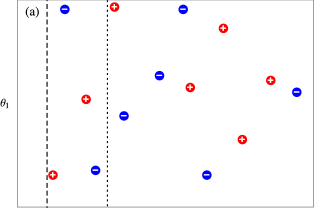
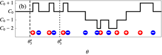
Figure 1: Weyl points and the change of Chern numbers. (a) the positive (red) and negative (blue) Weyl points in the ${\bm{\theta}}$ space and the integration planes used to compute $C(\theta^{\vphantom{*}}_{3})$ at $\theta_{3}=\theta_{3}^{a,b}$; the $\theta_{2}$ direction is omitted for ease of plotting. (b) the Weyl point distribution projected to the $\theta_{3}$ axis, where the Weyl points coincide with the change in the Chern number; $C_{0}$ denotes the initial value.

Since the Chern numbers only change at band-touching points because of topological protection, their dependences on $\theta_{3}$ are closely related to the distribution of Weyl points. To illustrate, Fig. 1 shows Weyl points distributed in the momentum space, and the constant $\theta_{3}$ planes (2-tori) over which the Berry curvature is integrated to compute the Chern number. For example, the integration plane for $C^{\vphantom{*}}_{n}(\theta^{\vphantom{\prime}}_{3})$ and $S^{\vphantom{*}}_{n}(\theta^{\vphantom{\prime}}_{3})$ is represented by the dotted line in Fig. 1. Moving the plane past Weyl point would increase (decrease) the Chern number by $1$, which determines its polarity to be positive (negative). The $\theta_{3}$ coordinates of the Weyl points coincide with the those $\theta_{3}$ at which the Chern number changes, as shown in Fig.1, which bears apparent similarity to random walk. Denoting the signed density of monopoles (Weyl points) between band $n$ and $n+1$ as $\rho_{n}({\bm{\theta}})=\rho_{n}^{+}({\bm{\theta}})-\rho_{n}^{-}({\bm{\theta}})$, the Chern number change is exactly the total signed number of monopoles between the plane $\theta_{3}=0$ and $\theta_{3}=\chi$, we have

$$\Delta C_{n}(\chi)\equiv C_{n}(\chi)-C_{n}(0)\\ =\int\limits_{0}^{\chi}\!d\theta_{3}\>\big{[}\lambda_{n}(\theta^{\vphantom{*}}_{3})-\lambda_{n-1}(\theta^{\vphantom{*}}_{3})\big{]}\quad,$$ (8)

where $\lambda_{n}(\theta^{\vphantom{*}}_{3})=\sum_{\sigma}\sigma\,\lambda^{\sigma}_{n}(\theta^{\vphantom{*}}_{3})$, with

$$\lambda_{n}^{\sigma}(\theta^{\vphantom{*}}_{3})=\int\limits_{0}^{2\pi}\!d\theta_{1}\int\limits_{0}^{2\pi}\!d\theta_{2}\ \rho_{n}^{\sigma}(\theta_{1},\theta_{2},\theta_{3})$$ (9)

the one-dimensional monopole (Weyl point) density. Similarly, the Fermi-level Chern number is given by $\Delta S_{n}(\chi)=S_{n}(\chi)-S_{n}(0)$.

2.2 Parametric GUE model

As we are interested in generic features of Weyl points and Chern numbers, we eschew attempts to model real materials and instead settle on a convenient model, which is that proposed by Walker and Wlikinson [13],

$$H({\bm{\theta}})={1\over\sqrt{3}}\sum_{r=1}^{3}\Big{[}\cos\theta^{\vphantom{*}}_{r}\,H^{(2r-1)}+\sin\theta^{\vphantom{*}}_{r}\,H^{(2r)}\Big{]}\quad,$$ (10)

where each of $\{H^{(1)},\ldots,H^{(6)}\}$ are independently drawn from the Gaussian unitary ensemble (GUE) of $M\times M$ matrices, with variances

$${\big{\langle}}(\textsf{Re}\,H_{ab})^{2}{\big{\rangle}}=1+\delta_{ab}\qquad,\qquad{\big{\langle}}(\textsf{Im}\,H_{ab})^{2}{\big{\rangle}}=1-\delta_{ab}\quad.$$ (11)

The statistics of $H({\bm{\theta}})$ and the derivative $\partial H/\partial\theta_{\alpha}$, for each ${\bm{\theta}}$, are GUE as well [13]. Therefore, computation at and perturbation around each momentum value ${\bm{\theta}}$ follow from well-known results of the GUE. The complex matrix $H({\bm{\theta}})$ depends on three parameters, hence according to the Wigner-von Neumann theorem we expect point degeneracies in the $3$-torus $(\theta_{1},\theta_{2},\theta_{3})$, with each $\theta_{\alpha}\in[0,2\pi)$. We call the parameterized ensemble of random matrices $H({\bm{\theta}})$ the Walker-Wilkinson ensemble (WWE).

The structure factor ${\hat{f}}({\bm{\vartheta}})$ for the WWE is given by

$${\hat{f}}^{\vphantom{*}}_{{\scriptscriptstyle\rm WWE}}({\bm{\vartheta}})={\textstyle{1\over 3}}\big{(}\cos\vartheta^{\vphantom{*}}_{1}+\cos\vartheta^{\vphantom{*}}_{2}+\cos\vartheta^{\vphantom{*}}_{3}\big{)}\quad;$$ (12)

note the normalization ${\hat{f}}(\bm{0})=1$. We shall also discuss the properties of a one-parameter extension of the WWE, given by

$$H({\bm{\theta}})=\sqrt{1-\alpha}\,H^{(0)}+{\sqrt{\alpha\over 3}}\sum_{r=1}^{3}\Big{[}\cos\theta^{\vphantom{*}}_{r}\,H^{(2r-1)}+\sin\theta^{\vphantom{*}}_{r}\,H^{(2r)}\Big{]}\quad,$$ (13)

where $\alpha\in[0,1]$ and where the seven matrices $\{H^{(1)},\ldots,H^{(7)}\}$ are independently chosen from the GUE. The corresponding structure factor is

$${\hat{f}}^{\vphantom{*}}_{\alpha{{\scriptscriptstyle\rm-WWE}}}({\bm{\vartheta}})=1-\alpha+{\alpha\over 3}\big{(}\cos\vartheta^{\vphantom{*}}_{1}+\cos\vartheta^{\vphantom{*}}_{2}+\cos\vartheta^{\vphantom{*}}_{3}\big{)}\quad,$$ (14)

which is again normalized. At $\alpha=0$, there is no dependence on the parameters $(\theta^{\vphantom{*}}_{1},\theta^{\vphantom{*}}_{2},\theta^{\vphantom{*}}_{3})$ and no degeneracies are induced by varying ${\bm{\theta}}$. All the Chern numbers are zero. As $\alpha$ increases toward $\alpha=1$ and we approach the WWE, monopoles appear, corresponding to degeneracies between neighboring bands, which lead to increases and decreases of Chern number.

From the WWE parametric random matrix model, we may compute the statistics of the Weyl points and Chern numbers, such as the densities $\rho_{n}^{\pm}({\bm{\theta}})$ and $\lambda^{\pm}_{n}(\theta^{\vphantom{*}}_{3})$ and the corresponding correlation functions ${\big{\langle}}\rho_{n}^{\sigma}({\bm{\theta}})\,\rho_{n^{\prime}}^{\sigma^{\prime}}({\bm{\theta}}^{\prime}){\big{\rangle}}$ and ${\big{\langle}}\lambda^{\sigma}_{n}(\theta^{\vphantom{*}}_{3})\,\lambda^{\sigma^{\prime}}_{n^{\prime}}(\theta^{\prime}_{3}){\big{\rangle}}$. The Chern number fluctuations are given by eqn. 8. We consider the fluctuations of ${\big{\langle}}[\Delta C_{n}(\chi)]^{2}{\big{\rangle}}$ and ${\big{\langle}}[\Delta S_{n}(\chi)]^{2}{\big{\rangle}}$ with respect to $\chi$ (the integration limit of $\theta_{3}$). Furthermore, we expand on the relation between the Weyl point distribution and Chern number fluctuation mentioned above, since they can serve as consistency check for our numerical data and analytical calculations.

Computation of the Chern number fluctuations thus requires the knowledge of the monopole correlations, which will be presented in later sections. Here we discuss some limiting cases that can be readily computed. For small $\chi$ limit, it has been shown that the fluctuation behaves like random walk with linear dispersion,

$${\big{\langle}}[\Delta C_{n}(\chi)]^{2}{\big{\rangle}}={1\over\pi}\big{(}N^{\pm}_{n}+N^{\pm}_{n-1}\big{)}\,\chi+{\cal O}(\chi^{2})\quad,$$ (15)

and

$${\big{\langle}}\big{[}\Delta S^{\vphantom{*}}_{n}(\chi)\big{]}^{2}{\big{\rangle}}={1\over\pi}\,N^{\pm}_{n}\,\chi+{\cal O}(\chi^{2})\quad,$$ (16)

with $N_{n}^{\sigma}=\iiint\rho_{n}^{\sigma}({\bm{\theta}})\>d^{3}\theta$ the total number of polarity $\sigma$ Weyl points between bands $n$ and $n+1$. Note $N_{n}^{+}=N_{n}^{-}\equiv N^{\pm}_{n}$. As discussed by Walker and Wilkinson [13], the Weyl point correlations only make higher order contributions to the fluctuation for small $\chi$. The derivation is reproduced in Appendix.A for convenience. For larger $\chi$, the correlations would make finite contributions and the fluctuation deviates from linearity. As a reference to contrast with numerical data, we compute the fluctuation with Weyl points treated as if independently distributed. The result is shown in Appendix.A to be a parabola:

$${\big{\langle}}\left[\Delta C_{n}(\chi)\right]^{2}{\big{\rangle}}={1\over\pi}\big{(}N^{\pm}_{n}+N^{\pm}_{n-1}\big{)}\,\chi\,\Big{(}1-{\chi\over 2\pi}\Big{)}\qquad,\qquad{\big{\langle}}\left[\Delta S_{n}(\chi)\right]^{2}{\big{\rangle}}={1\over\pi}\,N^{\pm}_{n}\,\chi\,\Big{(}1-{\chi\over 2\pi}\Big{)}\quad.$$ (17)

This starts out linearly for small $\chi$ as a random walk, and eventually returns to $\langle(\Delta C^{\vphantom{*}}_{n})^{2}\rangle=0$ at $\chi=2\pi$ because of periodicity. The presence of correlations will manifest in deviation from this result.

2.3 Method of locating Weyl points

To locate the Weyl points, we divide the three dimensional parameter space of $\left(\theta_{1},\theta_{2},\theta_{3}\right)$ into fine enough cells so that most of them contain at most a single Weyl point. The Berry curvature flux of each cell is computed, and the presence and polarity of the Weyl point is detected by the nonzero flux and its sign, respectively. We adopt the algorithm of [21] for the numerical method, where the flux through each plaquette is computed by the logarithm of the Wilson loop of around it, which guarantees the computed flux through a closed surface to be an integer and converges for modest grid resolution. The fluctuation of the Chern numbers is then obtained from the results of §2.1.

3 Numerical Result

In this section, we present numerical results of the Chern numbers fluctuation and the correlation of Weyl points. Our data shows that the Chern number fluctuation saturates at a plateau after initial linear growth, and there is short-range correlation between opposite polarity Weyl points. We also find a scaling relation of the saturation level of the Chern number fluctuation with respect to the total number of bands, which complements the scaling of the number of Weyl points discussed in previous work [13].

3.1 Diffusive behavior of the Chern number

As shown in Fig. 2, the fluctuation of Chern numbers $(\Delta C_{n})^{2}$ and $(\Delta S_{n})^{2}$ are evidently different from the parabola in (17) where correlations are ignored.

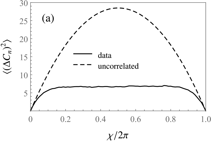
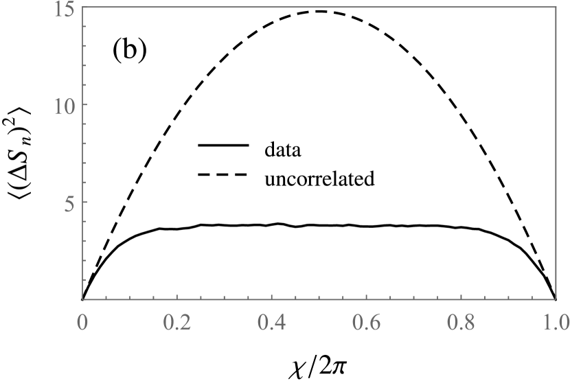
Figure 2: The fluctuations (a) $\langle\Delta C_{n}(\chi)^{2}\rangle$ and (b) $\langle\Delta S_{n}\left(\chi\right)^{2}\rangle$ for the parametric GUE model (solid line) compared with the hypothetical case where the correlations between the Weyl points are ignored (dashed). The data shown are obtained from the $n=4$ band, where the total number of bands $M=10$.

While the fluctuations do start linearly at small $\chi$, they eventually saturate at a plateau. This indicates the presence of correlation between Weyl points, which is discussed below. In addition to the data shown here, we have checked other energy bands and different system sizes with total number of bands from $M=10$ to 60. They all exhibit the same behavior, only with different plateau height and the value of $\theta_{3}$ at which the fluctuation saturates.

3.2 Correlation of Weyl points

We show the one-dimensional correlation function $\langle\lambda_{n}^{\sigma}(\theta^{\vphantom{*}}_{3})\,\lambda^{\sigma^{\prime}}_{n^{\prime}}(\theta^{\prime}_{3})\rangle$ as it is most directly linked to the Chern number as discussed in §2.1, where $\lambda_{n}^{\sigma}(\theta^{\vphantom{*}}_{3})$ is the linear monopole density defined in (9). The correlation between opposite-polarity and same-polarity Weyl points are shown in Fig.4.

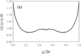
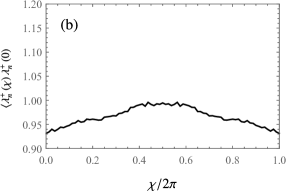
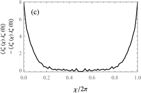
Figure 3: The correlation functions of (a) opposite-polarity points ${\big{\langle}}\lambda_{n}^{+}(\chi)\,\lambda_{n}^{-}(0){\big{\rangle}}$, (b) same-polarity points $\left\langle\lambda_{n}^{+}(\chi)\,\lambda_{n}^{+}(0)\right\rangle$, and (c) the difference $\left\langle\lambda_{n}^{+}(\chi)\,\lambda_{n}^{+}(0)\right\rangle-{\big{\langle}}\lambda_{n}^{+}(\chi)\,\lambda_{n}^{-}(0){\big{\rangle}}$, normalized so that they integrate to one. Data drawn from band $n=4$ and total number of bands $M=10$.

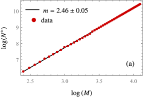
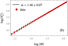
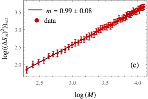
Figure 4: The scaling of (a) total number of Weyl points for all levels $\langle N^{\pm}\rangle\equiv\sum_{n}\langle N_{n}^{\pm}\rangle$, (b) the number of Weyl points for a single level $\langle N_{n}^{\pm}\rangle$, and (c) the plateau height for a single level ${\big{\langle}}\big{[}S_{n}(\chi)\big{]}^{2}{\big{\rangle}}^{\vphantom{\dagger}}_{\rm sat}$, versus the total number of bands f size $M$. The error bars in (a) are smaller than the data dots and not shown. The single levels are chosen at a fixed level with respect to the total number of bands, $n=0.4M$.

There is evident short-range correlation in the former, which is preserved in the difference $\left\langle\lambda_{n}^{+}(\theta^{\vphantom{*}}_{3})\,\lambda_{n}^{+}(0)\right\rangle-\left\langle\lambda_{n}^{+}(\theta^{\vphantom{*}}_{3})\,\lambda_{n}^{-}(0)\right\rangle$, that directly leads to the Chern number fluctuation $(\Delta C^{\vphantom{\prime}}_{n})^{2}$, also shown in Fig. 4. On the other hand, while correlations for Weyl points between different bands ${\big{\langle}}\rho_{n}^{\sigma}({\bm{\theta}})\,\rho_{n^{\prime}}^{\sigma^{\prime}}({\bm{\theta}}^{\prime}){\big{\rangle}}$ also contribute to the single level Chern number $C_{n}$, however our data in Appendix.C shows that for the different band correlation, the same polarity and opposite polarity pieces cancel each other, making no contribution to the Chern number fluctuation.

3.3 Scaling relations

Several scaling relations can be extracted from our numerical data. First, we reproduce the previously known scaling relation of the total number of Weyl points with respect to the total number of bands $M$ [13], $\sum_{n=1}^{M-1}N_{n}^{\pm}\propto M^{5/2}$ shown in Fig. 4. The average number of Weyl points per level should then scale as $N_{n}^{\pm}\propto M^{3/2}$, and one might suspect that this scaling also applies to the number for a fixed band $g_{n}$, which is indeed verified in Fig. 4. Moreover, we find another scaling relation for the height of the Chern number fluctuation plateau, ${\big{\langle}}\big{[}S^{\vphantom{\dagger}}_{n}(\chi)\big{]}^{2}{\big{\rangle}}^{\vphantom{\dagger}}_{\rm sat}\propto M^{1}$, as shown in Fig. 4. This also reflects the scaling relation for the correlation length, which we discuss in the following section. To make a fixed band index $n$ well-defined in the large $M$ limit, we choose the one at a fixed ratio to the total number of bands, i.e. $r=n/M$ fixed, although the scaling behaviors we discussed are insensitive to the choice of the ratio $r$.

4 Analytical interpretation

Having presented the numerical result, we discuss several different ways, in increasing rigor, to understand the short-range correlation between Weyl points and the fluctuation plateau. First, a qualitative picture which connects the two is illustrated; then the scaling relation of the correlation length is computed by perturbation theory, leading to the scaling exponent of the fluctuation plateau height. Finally, the entire functional form of the Chern number fluctuation is derived under the assumption that the short-range correlation function is exponential, which fits the data well.

4.1 Short-range correlation results in the saturation of the Chern number fluctuation

Here we provide a qualitative picture showing that the short-range correlation between opposite-polarity Weyl points results in the saturation plateau of Chern number fluctuation. Because of the short-range correlation, an opposite-polarity point would likely be present within the correlation length $\kappa$ apart from a particular Weyl point, while farther Weyl points are uncorrelated, as illustrated in Fig. 5.

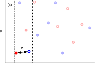
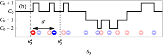
Figure 5: Correlated opposite polarity Weyl points shown as blue and hollow points at $\kappa$ apart, with other uncorrelated ones shown in lighter colors. The bottom plot shows the one-dimensional distribution and the change in the Chern number.

Now consider a $\theta^{\vphantom{*}}_{3}$ plane and compare the Chern number $C(\theta^{\vphantom{*}}_{3})$ to that on another plane $C(\theta^{\prime}_{3})$, where the difference is contributed by the Weyl points located in the region between the two planes. Increasing the separation $\Delta\theta_{3}$ from zero adds new points to the region and changes the Chern number. For $\Delta\theta^{\vphantom{*}}_{3}\equiv\theta^{\prime}_{3}-\theta^{\vphantom{\prime}}_{3}\ll\kappa$, most of the the short-range correlated points still locate outside the region, and the included points are uncorrelated. The fluctuation thus follows a random walk, growing linearly with the number of Weyl points. If we project the Weyl points to focus only on the $\theta_{3}$ coordinate, as shown in Fig. 5, the points within $\Delta\theta_{3}\ll\kappa$ are in fact separated in the $\theta_{1}$, $\theta_{2}$ direction and uncorrelated. When $\Delta\theta_{3}\gg\kappa$, the correlated opposite-polarity points will be added to the region, which cancels with existing contribution, so the fluctuation ceases to grow. The saturated value is reached by the total linear growth from the $\Delta\theta_{3}<\kappa$ range, determined by the number of Weyl points within this region:

$$\Big{\langle}\big{(}\Delta C_{n}\big{)}^{2}\Big{\rangle}_{\text{sat}}\propto{1\over\pi}\,\big{(}N^{\pm}_{n}+N^{\pm}_{n-1}\big{)}\,\kappa\qquad,\qquad{\big{\langle}}(\Delta S^{\vphantom{*}}_{n})^{2}{\big{\rangle}}^{\vphantom{\dagger}}_{\rm sat}\propto{1\over\pi}\,N^{\pm}_{n}\,\kappa\quad.$$ (18)

4.2 Perturbation theory calculation of the scaling relations

We now compute the scaling coefficient of the correlation length using perturbation theory. Expanding around an existing Weyl point, we solve for other nearby Weyl points and compute the expected distance $\kappa$ between them. This directly leads to the scaling coefficient of the fluctuation plateau height, which can be compared to our numerical data.

Consider perturbing the Hamiltonian around a particular Weyl point, taken to be of positive polarity and located at ${\bm{\theta}}=\left(0,0,0\right)$ without loss of generality. Assuming that the two bands are degenerate at zero energy (i.e. the energy reference is always shifted to the degenerate level), the Hamiltonian at the Weyl point in the diagonal basis takes the following form,

$$H_{0} =\begin{pmatrix}0_{2\times 2}&0_{2\times\left(M-2\right)}\\ 0_{\left(M-2\right)\times 2}&B_{0}\end{pmatrix}\quad,$$ (19)

where $B_{0}$ is a $\left(M-2\right)\times\left(M-2\right)$ diagonal matrix containing the the remaining energy bands. Away from the Weyl point, the Hamiltonian takes the general form of

$$\begin{split}H&=H_{0}+\begin{pmatrix}F^{\vphantom{\dagger}}_{1}&A^{\dagger}_{1}\\ A^{\vphantom{\dagger}}_{1}&B^{\vphantom{\dagger}}_{1}\end{pmatrix}\theta^{\vphantom{\prime}}_{1}+\begin{pmatrix}F^{\vphantom{\dagger}}_{2}&A^{\dagger}_{2}\\ A^{\vphantom{\dagger}}_{2}&B^{\vphantom{\dagger}}_{2}\end{pmatrix}\theta^{\vphantom{\prime}}_{2}+\begin{pmatrix}F^{\vphantom{\dagger}}_{3}&A^{\dagger}_{3}\\ A^{\vphantom{\dagger}}_{3}&B^{\vphantom{\dagger}}_{3}\end{pmatrix}\theta^{\vphantom{\prime}}_{3}+{\cal O}({\bm{\theta}}^{2})\\ &=\begin{pmatrix}{\bm{F}}\cdot{\bm{\theta}}&{\bm{A}}^{\dagger}\cdot{\bm{\theta}}\\ {\bm{A}}\cdot{\bm{\theta}}&B^{\vphantom{\dagger}}_{0}+{\bm{B}}\cdot{\bm{\theta}}\end{pmatrix}+{\cal O}({\bm{\theta}}^{2})\quad,\end{split}$$ (20)

where $F_{1,2,3}$ and $B_{1,2,3}$ are random Hermitian matrices and $A_{1,2,3}$ are random complex rectangular matrices. By perturbation theory, we can obtain the effective Hamiltonian in the first $2\times 2$ block,

$$H_{\rm eff}={\bm{F}}\cdot{\bm{\theta}}-({\bm{\theta}}\cdot{\bm{A}})^{\dagger}\,B_{0}^{-1}\,({\bm{\theta}}\cdot{\bm{A}})\quad,$$ (21)

which may be expanded in the Pauli basis, viz.

$$H^{\vphantom{*}}_{\rm eff}=\big{(}v^{\vphantom{*}}_{ai}\,\theta^{\vphantom{*}}_{i}-c^{\vphantom{*}}_{aij}\,\theta^{\vphantom{*}}_{i}\,\theta^{\vphantom{*}}_{j}\big{)}\,\sigma^{a}\quad,$$ (22)

with coefficients given by $v^{\vphantom{*}}_{ai}={\textstyle{1\over 2}}\textsf{Tr}\,\big{(}\sigma^{a}\,F^{\vphantom{*}}_{i}\big{)}$ and $c^{\vphantom{*}}_{aij}={\textstyle{1\over 2}}\textsf{Tr}\,\big{(}\sigma^{a}\,A^{\dagger}_{i}\,B_{0}^{-1}\,A^{\vphantom{\dagger}}_{j}\big{)}$. We then solve $\textsf{det}\,H({\bm{\theta}})=0$ to obtain the roots ${\bm{\theta}}={\bm{\theta}}^{*}$, which are the locations of the nearby Weyl points. These solutions ${\bm{\theta}}^{*}$ must contain as many positive and negative Weyl points, since the Chern numbers must sum to zero for the two energy bands of $H_{\rm eff}$. One of them is the original degeneracy point ${\bm{\theta}}^{*}=0$, thus the rest must consist of exactly one more point with polarity opposite to that of the original one than ones with the same polarity. From Bézout’s theorem, there are then at most eight point solutions to the three second-order equations in the three variables ${\bm{\theta}}^{*}$. However, numerical test shows that there are typically only two or four such solutions.

As $v_{ai}$ does not scale with system size, the scaling of ${\bm{\theta}}^{*}$ can be estimated from that of the coefficients $c_{aij}$, which is still difficult to compute. We therefore simplify $H_{\rm eff}$ by assuming that the only significant contribution to $B_{0}^{-1}$ in (19) is from the closest nondegenerate band, with energy $E_{\rm nd}$, ignoring all other contributions. Then

$$H_{\rm eff}={\bm{F}}\cdot{\bm{\theta}}-{({\bm{A}}^{\dagger}\cdot{\bm{\theta}})({\bm{A}}\cdot{\bm{\theta}})\over E^{\vphantom{*}}_{\rm nd}}\quad.$$ (23)

Thus, $\kappa\propto 1/c^{\vphantom{*}}_{abc}\propto E^{\vphantom{*}}_{\rm nd}$ . Since the Hamiltonian is derived from the GUE ensemble, $E^{\vphantom{*}}_{\rm nd}$ follows Wigner’s surmise [14]

$$P(s)={\textstyle{32\over\pi^{2}}}\,s^{2}e^{-4s^{2}/\pi}\quad,$$ (24)

where $s=E^{\vphantom{*}}_{\rm nd}/D$, with $D$ mean distance between energy levels. Assuming that $E^{\vphantom{*}}_{\rm nd}$ and the entries in $A$ are independent, we have

$$\textsf{var}(c^{-1})\propto\mathbb{E}\big{[}E^{2}_{\rm nd}\big{]}={\textstyle{1\over 2}}D^{2}\,\mathbb{E}(s^{2})={\textstyle{3\pi\over 16}}\,D^{2}\quad,$$ (25)

with $D=W/M$, $M$ the number of levels (the matrix size) and $W$ the spectral width. Under the semicircular law, $W=4\sqrt{M}$, so $D=4/\sqrt{M}$ and $\textsf{var}(c^{-1})\propto M$, leading to the scaling of the correlation length with respect to system size, $\kappa\propto M^{-1/2}$. Note that the only relevant scaling comes from the mean distance between energy levels $D$, while the functional form of Wigner’s surmise simply yields a dimensionless constant. Plugging this into (18), we obtain ${\big{\langle}}\big{[}\Delta S^{\vphantom{*}}_{n}(\chi)\big{]}^{2}{\big{\rangle}}^{\vphantom{*}}_{\rm sat}\propto M^{1}$ and similarly ${\big{\langle}}\big{[}\Delta C^{\vphantom{*}}_{n}(\chi)\big{]}^{2}{\big{\rangle}}^{\vphantom{*}}_{\rm sat}\propto M^{1}$, which agrees with the numerical scaling exponent shown in Fig. 4, where we find numerically a scaling exponent of $0.99\pm 0.08$.

4.3 Analytical derivation of the fluctuation plateau

Having computed the scaling relation for the correlation length, we calculate the Chern number fluctuation analytically for arbitrary $\Delta\theta_{3}$. We assume that the short range correlation functions of ${\big{\langle}}\rho_{n}^{+}(\bm{0})\,\rho_{n}^{-}({\bm{\theta}}){\big{\rangle}}$ decay exponentially, proportional to $e^{-|{\bm{\theta}}|/\kappa}$ (or, more accurately, a periodic version thereof), with the correlation length $\kappa=\kappa^{\vphantom{\dagger}}_{0}\,M^{-1/2}$ following the scaling relation $\kappa\propto M^{-1/2}$. Plugging this into our previous expressions, we obtain the closed form result for ${\big{\langle}}\big{[}\Delta S^{\vphantom{*}}_{n}(\chi)\big{]}^{2}{\big{\rangle}}$, derived in Appendix A:

$${\big{\langle}}\big{[}\Delta S^{\vphantom{\prime}}_{n}(\chi)\big{]}^{2}{\big{\rangle}} \approx-{\langle N^{\pm}_{n}\rangle\over\gamma^{\vphantom{\prime}}_{n}}\,\Bigg{\{}\big{[}2{\bar{\chi}}-3+(3+{\bar{\chi}})\,e^{-{\bar{\chi}}}\big{]}+{2\over\exp(\gamma^{\vphantom{\prime}}_{n})-1}\,\Big{(}1+{\gamma^{\vphantom{\prime}}_{n}\over 1-\exp(-\gamma^{\vphantom{\prime}}_{n})}\Big{)}\big{[}\cosh{\bar{\chi}}-1\big{]}$$ (26)

$$\hskip 180.67499pt-{2\over\exp(\gamma^{\vphantom{\prime}}_{n})-1}\>\big{[}{\bar{\chi}}\sinh{\bar{\chi}}-2\cosh{\bar{\chi}}+2\big{]}\Bigg{\}}+\langle N^{\pm}_{n}\rangle\,{\chi\over\pi}\quad,$$

where ${\bar{\chi}}=\chi/\kappa^{\vphantom{\prime}}_{n}$ and $\gamma^{\vphantom{\prime}}_{n}=2\pi/\kappa^{\vphantom{\prime}}_{n}$. The result agrees with the numerical data well, as shown in Fig. 6.

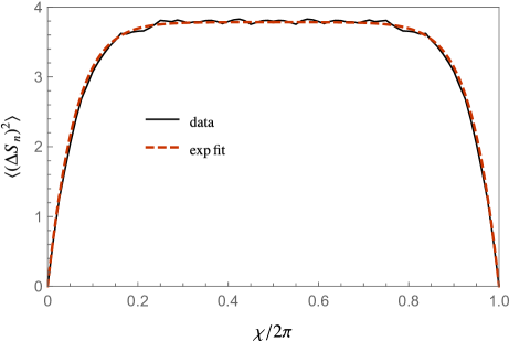
Figure 6: The Chern number fluctuation derived from the exponential correlation function compared with data.

The limits $\chi\ll\kappa$ and $\chi\gg\kappa$ can also be found, which shows linear growth of random walk and saturation plateau, respectively,

$${\big{\langle}}\big{[}\Delta S^{\vphantom{*}}_{n}(\chi)\big{]}^{2}{\big{\rangle}}\approx\begin{cases}N^{\pm}_{n}\chi/\pi&{\rm if}\ \chi\ll\kappa\\ 3N^{\pm}_{n}\kappa/2\pi&{\rm if}\ \chi\gg\kappa\quad.\end{cases}$$ (27)

The saturation value is obtained in the $\kappa\ll 1$ limit from eqn. 43. The scaling of the plateau height can be obtained from that of the number of degeneracies, $N^{\vphantom{*}}_{n}=g^{\vphantom{\dagger}}_{0}\,M^{3/2}$, and the correlation length $\kappa=\kappa^{\vphantom{\dagger}}_{0}\,M^{-1/2}$, where $g^{\vphantom{\dagger}}_{0}$ and $\kappa^{\vphantom{\dagger}}_{0}$ are constants. We then have

$${\big{\langle}}\big{[}\Delta S^{\vphantom{*}}_{n}(\chi)\big{]}^{2}{\big{\rangle}}^{\vphantom{\dagger}}_{\rm sat}={3\over 2\pi}\,g^{\vphantom{*}}_{0}\,\kappa^{\vphantom{*}}_{0}\,M\quad,$$ (28)

which agrees with the linear scaling with the total number of bands $M$ of our data in Fig. 4. For the single level Chern number $\left<(\Delta C_{n})^{2}\right>$, the fluctuation involves correlations across different bands ${\big{\langle}}\lambda_{n}^{\sigma}(\theta^{\vphantom{*}}_{3})\,\lambda_{n-1}^{\sigma}(\theta^{\prime}_{3}){\big{\rangle}}$. Though we do not have an analytical understanding of this term, our numerical data in Appendix. C shows that its net contribution to the fluctuation is negligible, so we arrive at a similar expression

$${\big{\langle}}\big{[}\Delta C^{\vphantom{*}}_{n}(\chi)\big{]}^{2}{\big{\rangle}}\approx\begin{cases}\big{(}N^{\pm}_{n}+N^{\pm}_{n-1}\big{)}\chi/\pi&{\rm if}\ \chi\ll\kappa\\ 3\big{(}N^{\pm}_{n}+N^{\pm}_{n-1}\big{)}\kappa/2\pi&{\rm if}\ \chi\gg\kappa\quad.\end{cases}\quad.$$ (29)

That the analytical result fits the numerical data well supports the validity of our qualitative picture and the perturbation theory calculation. Other ansatzes for the correlation function are also considered in Appendix.A, among which the exponential decay considered here produces the best fit.

5 Result for the one-parameter extension of Walker-Wilkinson ensemble

For completeness, we also show the result for the one-parameter extension of WWE discussed in 13, where the parameter $\alpha$ interpolates between the WWE and a Hamiltonian independent of the parameters. Fig. 7

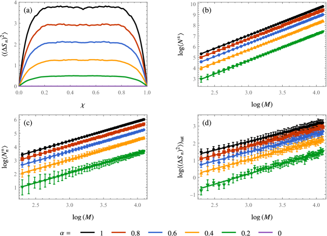
Figure 7: Numerical results for the one-parameter extension of WWE discussed in 13, with (a) the fluctuation of Chern numbers for the level $n=4$ of system size $M=10$, and the scaling w.r.t. system size of (b) total number of degeneracy points, (c) number of degeneracy points at a single level, and (d) the saturation of Chern number fluctuation. The scaling exponents for different $\alpha$, shown in Table. 1, agrees with $\alpha=1$.

	1	0.8	0.6	0.4	0.2
$\langle N^{\pm}\rangle$	$2.47\pm 0.04$	$2.46\pm 0.04$	$2.46\pm 0.05$	$2.47\pm 0.06$	$2.47\pm 0.09$
$\langle N^{\pm}_{n}\rangle$	$1.45\pm 0.07$	$1.44\pm 0.08$	$1.44\pm 0.09$	$1.45\pm 0.1$	$1.44\pm 0.2$
$\langle\left(\Delta S_{n}\right)^{2}\rangle$	$1.01\pm 0.1$	$1.03\pm 0.1$	$1.06\pm 0.1$	$1.08\pm 0.1$	$1.19\pm 0.1$

Table 1: The scaling exponents for the number of degeneracy points and Chern number fluctuation plateau height with respect to the system size $M$, plot presented in Fig. 7

shows the numerical result, consistent with our prediction where tuning $\alpha$ from 1 to 0 reduces the number of degeneracy points and Chern number fluctuation. Note that the scaling coefficients remain the same for different $\alpha$, which can be traced back to the derivation in Sec.4, where the scaling coefficient comes solely from the semicircular law of the random matrix ensemble, and the one-parameter Hamiltonian still satisfies the Gaussian unitary ensemble statistics.

6 Discussion

In this work, we extended the analysis of a random matrix model with three parameters from Walker and Wilkinson [13] and investigated the Weyl points distribution in the parameter space and the fluctuation of Chern numbers. Our numerical data shows that there is short-ranged correlation between opposite-polarity degeneracy points, and that the Chern number fluctuation, known to linear disperse for small $\Delta\theta_{3}$ [13], eventually saturates at a plateau. A scaling relation for the height of such plateau with respect to the total number of bands is also found, complementing the already known scaling relation for the total number of Weyl points. To explain this result, we first provided a qualitative argument that connected the short-range correlation to the saturation of the Chern number fluctuation. Then, perturbation theory is utilized to quantitatively compute the scaling exponent. Finally, postulating that the short-range correlation function is exponentially decaying, the Chern number fluctuation is analytically derived, which agrees with the numerical data. We also investigated a one-parameter family of models which interpolates between the Walker-Wilkinson ensemble and a constant Hamiltonian. Our numerics shows that the number of degeneracy points and Chern number fluctuation decreases when tuned away from the WWE, as expected.

Our result can potentially be applied to Weyl semimetal materials with many Weyl points in the bulk. The opposite-polarity Weyl points would tend to pair up due to the short-range correlation, and the expected numbers of Fermi arc states would be similar throughout most of the surface Brillouin zone, indicated by the saturation of the Chern number fluctuation. The scaling relations also indicates how much one can increase the number of Weyl poins and Fermi arc states by enlarging the system size.

Although the random matrix model adopted here is derived from the GUE ensemble, representing a generic system without any symmetry, our qualitative arguments and computation steps can be readily adapted to different random matrix ensembles. The Chern number fluctuation is related to the Weyl point correlations by simple integrals, and the perturbation theory calculation of the scaling can be modified to include the Wigner surmise for the appropriate ensemble. An example of this has been done in [19], where random matrices obeying the Bogoliubov-de-Gunnes mirror symmetry were considered to describe Weyl points in multichannel Josephson junctions. The band-touching points of different ensembles may have a different co-dimension and are associated with different topological invariant such as the second Chern number. We leave this direction to future work.

Appendix A Chern numbers from the location of degeneracies

Here we expand on the properties of the Weyl point correlation function and its consequences for Chern number fluctuations. The density $\rho_{n}^{\sigma}({\bm{\theta}})$ is given by

$$\rho_{n}^{\sigma}({\bm{\theta}})=\sum_{j=1}^{N^{\sigma}_{n}}{\tilde{\delta}}({\bm{\theta}}-{\bm{\theta}}^{\sigma}_{n,j})\quad,$$ (30)

where ${\bm{\theta}}^{\sigma}_{nj}$ is the location of the $j^{\rm th}$ Weyl point of polarity $\sigma$ between bands $n$ and $n+1$, and where ${\tilde{\delta}}({\bm{\theta}})=\sum_{\bm{l}}\delta({\bm{\theta}}-2\pi{\bm{l}})$ is periodic under displacement of the dimensionless wavevector ${\bm{\theta}}$ by any ${\bm{l}}=(l^{\vphantom{*}}_{1},l^{\vphantom{*}}_{2},l^{\vphantom{*}}_{3})$ is a triple of integers. For a given instantiation of $H({\bm{\theta}})$, the number of such Weyl points we define to be $N_{n}^{\sigma}$; clearly $N_{n}^{+}=N_{n}^{-}\equiv N^{\pm}_{n}$. However these numbers may fluctuate within our matrix ensemble. Thus this is a ‘grand canonical’ formulation. We then have

$$\begin{split}\Delta C^{\vphantom{\dagger}}_{n}(\chi)&=\int\limits_{\textsf{T}^{2}}\!d^{2}\theta^{\vphantom{*}}_{\perp}\!\int\limits_{0}^{\chi}\!d\theta^{\vphantom{*}}_{3}\>\sum_{\sigma}\sigma\,\Big{\{}\rho_{n}^{\sigma}({\bm{\theta}})-\rho_{n-1}^{\sigma}({\bm{\theta}})\Big{\}}\\ \Delta S^{\vphantom{\dagger}}_{n}(\chi)&=\sum_{j=1}^{n}C^{\vphantom{\dagger}}_{j}(\chi)=\int\limits_{\textsf{T}^{2}}\!d^{2}\theta^{\vphantom{*}}_{\perp}\!\int\limits_{0}^{\chi}\!d\theta^{\vphantom{*}}_{3}\ \sum_{\sigma}\sigma\,\rho_{n}^{\sigma}({\bm{\theta}})\quad,\end{split}$$ (31)

where ${\textsf{T}^{2}}$ denotes the 2-torus $[0,2\pi]\times[0,2\pi]$. ${\bm{\theta}}$-space translational invariance of the one- and two-point distributions entails

$${\big{\langle}}\rho_{n}^{\sigma}({\bm{\theta}}){\big{\rangle}}={\langle N^{\sigma}_{n}\rangle\over 8\pi^{3}}\qquad,\qquad{\big{\langle}}\rho_{n}^{\sigma}({\bm{\theta}})\,\rho_{n^{\prime}}^{\sigma^{\prime}}({\bm{\theta}}^{\prime}){\big{\rangle}}=F_{n,n^{\prime}}^{\sigma,\sigma^{\prime}}({\bm{\theta}}-{\bm{\theta}}^{\prime})\quad,$$ (32)

and we may write

$$F_{n,n^{\prime}}^{\sigma,\sigma^{\prime}}({\bm{\theta}}-{\bm{\theta}}^{\prime})={1\over 8\pi^{3}}\>\bigg{\{}\langle N^{\pm}_{n}\rangle\,\delta^{\vphantom{*}}_{\sigma,\sigma^{\prime}}\,\delta^{\vphantom{*}}_{n,n^{\prime}}\,{\tilde{\delta}}({\bm{\theta}}-{\bm{\theta}}^{\prime})+R_{n,n^{\prime}}^{\sigma,\sigma^{\prime}}({\bm{\theta}}-{\bm{\theta}}^{\prime})\bigg{\}}\quad,$$ (33)

where $R_{n,n^{\prime}}^{\sigma,\sigma^{\prime}}({\bm{\vartheta}})$ is regular, with no $\delta$-function singularities in ${\bm{\vartheta}}={\bm{\theta}}-{\bm{\theta}}^{\prime}$. Note the sum rule,

$$\int\limits_{\textsf{T}^{3}}\!d^{3}\vartheta\>R^{\sigma,\sigma^{\prime}}_{n,n^{\prime}}({\bm{\vartheta}})={\big{\langle}}N^{\sigma}_{n}\,N^{\sigma^{\prime}}_{n^{\prime}}{\big{\rangle}}-{\big{\langle}}N^{\sigma}_{n}{\big{\rangle}}\>\delta^{\vphantom{*}}_{n,n^{\prime}}\,\delta^{\vphantom{*}}_{\sigma,\sigma^{\prime}}\quad,$$ (34)

where ${\textsf{T}^{3}}$ denotes the three-dimensional torus. Note that $R^{\sigma,\sigma^{\prime}}_{n,n^{\prime}}({\bm{\vartheta}})$ is reflection symmetric under $q^{\vphantom{*}}_{\mu}\to-q^{\vphantom{*}}_{\mu}$ for $\mu\in\{1,2,3\}$. We thus have

$$\begin{split}{\big{\langle}}\big{[}\Delta C^{\vphantom{\prime}}_{n}(\chi)\big{]}^{2}{\big{\rangle}}&=\Big{(}\langle N^{\pm}_{n}\rangle+\langle N^{\pm}_{n-1}\rangle\Big{)}\,{\chi\over\pi}+2\int\limits_{0}^{\chi}\!d\alpha\!\!\int\limits_{0}^{\chi-\alpha}\!\!\!d\theta^{\vphantom{\prime}}_{3}\>\Big{(}\Lambda^{\parallel}_{n,n}(\theta^{\vphantom{*}}_{3})+\Lambda^{\parallel}_{n-1,n-1}(\theta^{\vphantom{*}}_{3})-2\Lambda^{\parallel}_{n,n-1}(\theta^{\vphantom{*}}_{3})\Big{)}\\ {\big{\langle}}\big{[}\Delta S^{\vphantom{\prime}}_{n}(\chi)\big{]}^{2}{\big{\rangle}}&=\langle N^{\pm}_{n}\rangle\,{\chi\over\pi}+2\int\limits_{0}^{\chi}\!d\alpha\!\!\int\limits_{0}^{\chi-\alpha}\!\!\!d\theta^{\vphantom{*}}_{3}\>\Lambda^{\parallel}_{n,n}(\theta^{\vphantom{*}}_{3})\quad,\end{split}$$ (35)

where

$$\Lambda^{\vphantom{\prime}}_{n,n^{\prime}}({\bm{\vartheta}})={1\over 2\pi}\sum_{\sigma,\sigma^{\prime}}\sigma\sigma^{\prime}\,R^{\sigma,\sigma^{\prime}}_{n,n^{\prime}}({\bm{\vartheta}})\qquad,\qquad\Lambda^{\parallel}_{n,n^{\prime}}(\vartheta^{\vphantom{*}}_{3})=\int\limits_{\textsf{T}^{2}}\!d^{2}\vartheta^{\vphantom{*}}_{\perp}\>\Lambda^{\vphantom{\prime}}_{n,n^{\prime}}({\bm{\vartheta}}^{\vphantom{*}}_{\perp},\vartheta^{\vphantom{*}}_{3})\quad.$$ (36)

If we assume that $R^{\sigma,\sigma^{\prime}}_{n,n^{\prime}}({\bm{\vartheta}})$ is independent of ${\bm{\vartheta}}$, i.e. the locations of different Weyl points are completely uncorrelated, then from the sum rule

$$\int\limits_{\textsf{T}^{3}}\!d^{3}\vartheta\ \Lambda^{\vphantom{\prime}}_{n,n^{\prime}}({\bm{\vartheta}})=-{1\over\pi}\,\langle N^{\pm}_{n}\rangle\,\delta^{\vphantom{*}}_{n,n^{\prime}}$$ (37)

we have the crude approximation

$$\Lambda^{\textsf{nc}}_{n,n^{\prime}}({\bm{\vartheta}})=-{1\over 8\pi^{4}}\,{\big{\langle}}N^{\pm}_{n}{\big{\rangle}}\,\delta^{\vphantom{*}}_{n,n^{\prime}}\quad,$$ (38)

from which we recover (17). Here the superscript nc stands for ‘no correlations’.

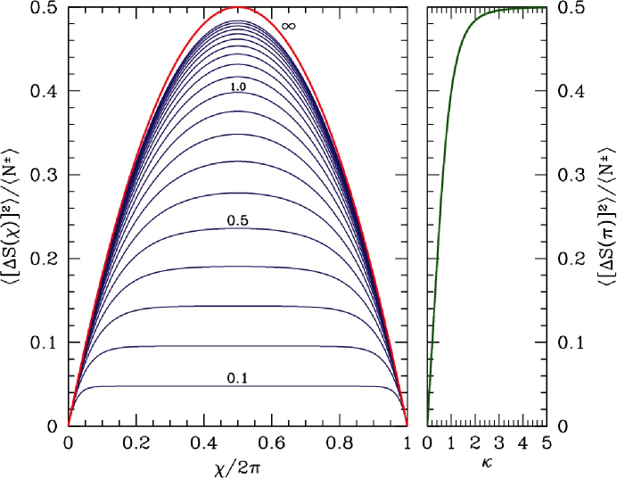
Figure 8: Predictions of the approximation formula eqn. 43 for the total Chern number fluctuation versus slab thickness $\chi$. Left: results for 20 equally spaced values of $\kappa$ and $\kappa=\infty$. Right: the values at $\chi=\pi$.

We now extend this analysis to include correlations among different Weyl points using a phenomenological description. Again imposing the sum rule constraint, we write

$$\Lambda^{\vphantom{\prime}}_{n,n^{\prime}}({\bm{\vartheta}})\approx-\delta^{\vphantom{\prime}}_{n,n^{\prime}}\ {{\big{\langle}}N^{\pm}_{n}{\big{\rangle}}\over 8\pi^{2}\kappa_{n}^{3}}\ \sum_{{\bm{l}}\in\mathbb{Z}^{3}}e^{-|{\bm{\vartheta}}-2\pi{\bm{l}}|/\kappa^{\vphantom{\prime}}_{n}}\quad,$$ (39)

where the sum on ${\bm{l}}$ is over all triples of integers. Integrating over $(\vartheta^{\vphantom{\prime}}_{1},\vartheta^{\vphantom{\prime}}_{2})$, we find

$$\Lambda^{\parallel}_{n,n^{\prime}}(\vartheta^{\vphantom{*}}_{3})=-\,\delta^{\vphantom{*}}_{n,n^{\prime}}\>{{\big{\langle}}N^{\pm}_{n}{\big{\rangle}}\over 4\pi\kappa^{\vphantom{\prime}}_{n}}\sum_{l=-\infty}^{\infty}\bigg{(}1+{|\vartheta^{\vphantom{*}}_{3}-2\pi l|\over\kappa^{\vphantom{\prime}}_{n}}\bigg{)}\,e^{-|\vartheta^{\vphantom{*}}_{3}-2\pi l|/\kappa^{\vphantom{\prime}}_{n}}\quad.$$ (40)

Our approximation results in

$${\big{\langle}}\big{[}\Delta S^{\vphantom{\prime}}_{n}(\chi)\big{]}^{2}{\big{\rangle}}\approx\langle N^{\pm}_{n}\rangle\,{\chi\over\pi}+2\int\limits_{0}^{\chi}\!d\alpha\!\!\int\limits_{0}^{\chi-\alpha}\!\!\!d\vartheta^{\vphantom{*}}_{3}\ \Lambda^{\parallel}_{n,n}(\vartheta^{\vphantom{*}}_{3})$$ (41)

and

$${\big{\langle}}\big{[}\Delta C^{\vphantom{\prime}}_{n}(\chi)\big{]}^{2}{\big{\rangle}}\approx{\big{\langle}}\big{[}\Delta S^{\vphantom{\prime}}_{n}(\chi)\big{]}^{2}{\big{\rangle}}+{\big{\langle}}\big{[}\Delta S^{\vphantom{\prime}}_{n-1}(\chi)\big{]}^{2}{\big{\rangle}}\quad.$$ (42)

The sums and integrals can be performed, yielding the following closed-form expression:

$${\big{\langle}}\big{[}\Delta S^{\vphantom{\prime}}_{n}(\chi)\big{]}^{2}{\big{\rangle}} \approx-{\langle N^{\pm}_{n}\rangle\over\gamma^{\vphantom{\prime}}_{n}}\,\Bigg{\{}\big{[}2{\bar{\chi}}-3+(3+{\bar{\chi}})\,e^{-{\bar{\chi}}}\big{]}+{2\over\exp(\gamma^{\vphantom{\prime}}_{n})-1}\,\Big{(}1+{\gamma^{\vphantom{\prime}}_{n}\over 1-\exp(-\gamma^{\vphantom{\prime}}_{n})}\Big{)}\big{[}\cosh{\bar{\chi}}-1\big{]}$$ (43)

$$\hskip 180.67499pt-{2\over\exp(\gamma^{\vphantom{\prime}}_{n})-1}\>\big{[}{\bar{\chi}}\sinh{\bar{\chi}}-2\cosh{\bar{\chi}}+2\big{]}\Bigg{\}}+\langle N^{\pm}_{n}\rangle\,{\chi\over\pi}\quad,$$

where ${\bar{\chi}}=\chi/\kappa^{\vphantom{\prime}}_{n}$ and $\gamma^{\vphantom{\prime}}_{n}=2\pi/\kappa^{\vphantom{\prime}}_{n}$ .

For completeness we also tested different functional form for the correlation function, including the Gaussian $\exp(-{\bm{\theta}}^{2}/\kappa)$, the quartic exponential $\exp\big{(}-|{\bm{\theta}}|^{4}/\kappa\big{)}$, and a hypothetical case where the one-dimensional correlation function is a step function, obtaining the resulting Chern number fluctuation. The results are shown in shown in Fig. 9,

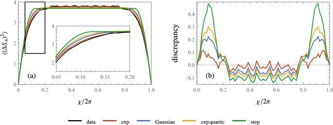
Figure 9: The predicted Chern number fluctuation obtained from correlation functions of different functional forms, (a) compared with data, and (b) the difference with data. The matrix rank is $M=10$.

where the existence of the saturation plateau does not depend on the correlation functional form, in agreement with the prediction in Sec.4.1, and that the exponential function adopted in the main text fits the numerical data best.

Appendix B Special cases for the Chern number fluctuations

Although the Chern number fluctuation for most energy band $n$ and different total numbers of bands $M$ obey the saturation pattern of Fig.2, there are some special symmetries to our ${\bm{\theta}}$-parameterized GUE which constrain the correlation functions. In addition to the periodicity $H({\bm{\theta}}+2\pi{\bm{l}})=H({\bm{\theta}})$, where ${\bm{l}}=(l^{\vphantom{*}}_{1},l^{\vphantom{*}}_{2},l^{\vphantom{*}}_{3})$ with each $l^{\vphantom{*}}_{\mu}\in\mathbb{Z}$, we also have $H({\bm{\theta}}+{\bm{\pi}})=-H({\bm{\theta}})$, where ${\bm{\pi}}=(\pi,\pi,\pi)$. This entails the relation $E^{\vphantom{*}}_{n}({\bm{\theta}}+{\bm{\pi}})=E^{\vphantom{*}}_{M+1-n}({\bm{\theta}})$, and thus $\rho^{\pm}_{n}({\bm{\theta}}+{\bm{\pi}})=\rho^{\mp}_{M-n}({\bm{\theta}})$. In most cases this symmetry does not manifest in the Chern number fluctuations, since it does not constrain the Weyl points for a given band. The exceptions are the cases $n=M/2$ for $M$ even and $n=(M+1)/2$ for $M$ odd, for which

$$\begin{split}\rho^{\pm}_{M/2}({\bm{\theta}}+{\bm{\pi}})&=\rho^{\mp}_{M/2}({\bm{\theta}})\qquad\quad\ \ \hbox{\rm($M$ even})\\ \rho^{\pm}_{(M+1)/2}({\bm{\theta}}+{\bm{\pi}})&=\rho^{\mp}_{(M-1)/2}({\bm{\theta}})\qquad\hbox{\rm($M$ odd)}\end{split}$$ (44)

Integrating over $\theta^{\vphantom{*}}_{1,2}$ we have that

$$\begin{split}\lambda^{\pm}_{M/2}(\theta^{\vphantom{*}}_{3}+\pi)&=\lambda^{\mp}_{M/2}(\theta^{\vphantom{*}}_{3})\qquad\quad\ \ \hbox{\rm($M$ even})\\ \lambda^{\pm}_{(M+1)/2}(\theta^{\vphantom{*}}_{3}+\pi)&=\lambda^{\mp}_{(M-1)/2}(\theta^{\vphantom{*}}_{3})\qquad\hbox{\rm($M$ odd)}\end{split}$$ (45)

for the one-dimensional distributions $\lambda_{\bar{n}}^{\sigma}(k)$, where ${\bar{n}}={\textstyle{1\over 2}}M$ for $M$ even and ${\bar{n}}={\textstyle{1\over 2}}(M+1)$ for $M$ odd. The Chern number change $\Delta C^{\vphantom{*}}_{\bar{n}}(\chi)$ is given in eqn. 8, and using the above results we have for $M$ odd that

$$\Delta C^{\rm odd}_{\bar{n}}(\chi)=\int\limits_{0}^{\chi}\!d\theta^{\vphantom{*}}_{3}\>\sum_{\sigma}\,\sigma\big{(}\lambda^{\sigma}_{\bar{n}}(\theta^{\vphantom{*}}_{3})+\lambda^{\sigma}_{\bar{n}}(\theta^{\vphantom{*}}_{3}+\pi)\big{)}\quad,$$ (46)

and therefore

$$\Delta C^{\rm odd}_{\bar{n}}(\pi)=\int\limits_{0}^{2\pi}\!d\theta^{\vphantom{*}}_{3}\>\sum_{\sigma}\sigma\,\lambda_{\bar{n}}^{\sigma}(\theta^{\vphantom{*}}_{3})=0\quad.$$ (47)

For $M$ even, we invoke

$${\big{\langle}}\big{[}\Delta C^{\vphantom{*}}_{n}(\chi)\big{]}^{2}{\big{\rangle}}=\int\limits_{0}^{\chi}\!d\theta^{\vphantom{*}}_{3}\int\limits_{0}^{\chi}\!d\theta^{\prime}_{3}\>\sum_{\sigma,\sigma^{\prime}}\sigma\sigma^{\prime}\,\Big{[}{\big{\langle}}\lambda_{n}^{\sigma}(\theta^{\vphantom{\prime}}_{3})\,\lambda_{n}^{\sigma^{\prime}}(\theta^{\prime}_{3}){\big{\rangle}}+{\big{\langle}}\lambda_{n-1}^{\sigma}(\theta^{\vphantom{\prime}}_{3})\,\lambda_{n-1}^{\sigma^{\prime}}(\theta^{\prime}_{3}){\big{\rangle}}-2\,{\big{\langle}}\lambda_{n}^{\sigma}(\theta^{\vphantom{\prime}}_{3})\,\lambda_{n-1}^{\sigma^{\prime}}(\theta^{\prime}_{3}){\big{\rangle}}\Big{]}$$ (48)

and

$$F^{\parallel}_{n,n^{\prime}}(\theta^{\vphantom{*}}_{3}-\theta^{\prime}_{3})\equiv\sum_{\sigma,\sigma^{\prime}}\sigma\sigma^{\prime}\,{\big{\langle}}\lambda^{\sigma}_{n}(\theta^{\vphantom{\prime}}_{3})\,\lambda^{\sigma^{\prime}}_{n^{\prime}}(\theta^{\prime}_{3}){\big{\rangle}}={1\over\pi}\,{\big{\langle}}N^{\pm}_{n}{\big{\rangle}}\>\delta^{\vphantom{*}}_{n,n^{\prime}}\,{\tilde{\delta}}(\theta^{\vphantom{\prime}}_{3}-\theta^{\prime}_{3})+\Lambda^{\parallel}_{n,n^{\prime}}(\theta^{\vphantom{\prime}}_{3}-\theta^{\prime}_{3})\quad,$$ (49)

where ${\tilde{\delta}}(\vartheta^{\vphantom{*}}_{3})=\sum_{l}\delta(\vartheta^{\vphantom{*}}_{3}-2\pi l)$. Invoking the symmetry under advancing $\vartheta^{\vphantom{\prime}}_{3}=\theta^{\prime}_{3}-\theta^{\vphantom{\prime}}_{3}$ by $\pi$, we may write

$$F^{\parallel}_{{\bar{n}},{\bar{n}}}(\vartheta^{\vphantom{*}}_{3})={1\over\pi}\,{\big{\langle}}N^{\pm}_{\bar{n}}{\big{\rangle}}\>\Big{(}{\tilde{\delta}}(\vartheta^{\vphantom{*}}_{3})-{\tilde{\delta}}(\vartheta^{\vphantom{*}}_{3}-\pi)\Big{)}+{\tilde{\Lambda}}^{\parallel}_{{\bar{n}},{\bar{n}}}(\vartheta^{\vphantom{*}}_{3})-{\tilde{\Lambda}}^{\parallel}_{{\bar{n}},{\bar{n}}}(\vartheta^{\vphantom{*}}_{3}-\pi)\quad,$$ (50)

where ${\tilde{\Lambda}}^{\parallel}_{{\bar{n}},{\bar{n}}}(\vartheta^{\vphantom{*}}_{3})$ is regular. Integrating over $\theta^{\vphantom{\prime}}_{3}$ and $\theta^{\prime}_{3}$ to obtain ${\big{\langle}}\big{[}\Delta C^{\vphantom{*}}_{n}(\chi)\big{]}^{2}{\big{\rangle}}$, we have

$${\big{\langle}}\big{[}\Delta C^{\vphantom{*}}_{\bar{n}}(\chi)\big{]}^{2}{\big{\rangle}}={\big{\langle}}N^{\pm}_{\bar{n}}{\big{\rangle}}\bigg{(}1-{|\chi-\pi|\over\pi}\bigg{)}+\ldots\quad,$$ (51)

where the first term on the RHS is due to the delta functions, and the terms included in the ellipses are smooth, periodic functions of $\chi$ which are symmetric about $\chi=\pi$. Thus, there is a downward cusp at $\chi=\pi$, as we observe in our simulations. The results for $M$ even and $M$ odd are shown in Fig. 10.

We stress that the cusps present at $\chi=\pi$ for the special bands ${\bar{n}}$ in the even and odd $M$ cases are nongeneric features which arise due to the Walker-Wilkinson parameterization of $H({\bm{\theta}})$ in eqn. 10.

Figure 10: The Chern number fluctuation of the middle energy band for (a) odd total number of bands (b) even total number of bands. Data from $n=6$ of odd total number of bands $M=11$ and $n=5$ of even total number of bands $M=10$, respectively.

Appendix C Weyl point correlations among different energy bands

In Fig. 11 we show the numerical result for the correlations of monopoles between different energy bands, ${\big{\langle}}\lambda_{n}^{\sigma}(\chi)\,\lambda_{n-1}^{\sigma^{\prime}}(0){\big{\rangle}}$.

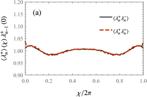
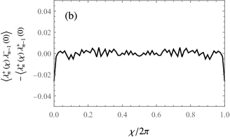
Figure 11: The correlation among Weyl points between different energy bands. (a) same-polarity correlation ${\big{\langle}}\lambda_{n}^{+}(\chi)\,\lambda_{n-1}^{+}(0){\big{\rangle}}$ and opposite-polarity correlation ${\big{\langle}}\lambda_{n}^{+}(\chi)\,\lambda_{n-1}^{-}(0){\big{\rangle}}$, (b) the difference ${\big{\langle}}\lambda_{n}^{+}(\chi)\,\lambda_{n-1}^{+}(0){\big{\rangle}}-{\big{\langle}}\lambda_{n}^{+}(\chi)\,\lambda_{n-1}^{-}(0){\big{\rangle}}$. The first two are normalized to integrate to one, while the last is the difference of the former two without further normalization. Data is obtained for system size $M=10$ and $n=4$.

which contribute to the fluctuation $\langle\left(\Delta C_{n}\right)^{2}\rangle$ in (35) but cannot be quantified by our perturbation description. Here, the numerical data shows that the difference ${\big{\langle}}\lambda_{n}^{+}(\chi)\,\lambda_{n-1}^{+}(0){\big{\rangle}}-{\big{\langle}}\lambda_{n}^{+}(\chi)\,\lambda_{n-1}^{-}(0){\big{\rangle}}$ effectively cancel out, making a negligible contribution to $\langle\left(\Delta C_{n}\right)^{2}\rangle$. Therefore, the behavior of $\langle\left(\Delta C_{n}\right)^{2}\rangle$ can be to good accuracy calculated from our perturbation theory analysis, as in (29), despite our neglect of correlation effects across different energy bands.

References

• [1] Xiangang Wan, Ari M. Turner, Ashvin Vishwanath, and Sergey Y. Savrasov. Topological semimetal and Fermi-arc surface states in the electronic structure of pyrochlore iridates. Physical Review B, 83(20):205101, 2011.
• [2] Vivek Aji. Adler-Bell-Jackiw anomaly in Weyl semimetals: Application to pyrochlore iridates. Physical Review B, 85(24):241101, 2012.
• [3] Pavan Hosur and Xiaoliang Qi. Recent developments in transport phenomena in Weyl semimetals. Comptes Rendus Physique, 14(9-10):857–870, 2013.
• [4] D. T. Son and B. Z. Spivak. Chiral anomaly and classical negative magnetoresistance of Weyl metals. Physical Review B, 88(10):104412, 2013.
• [5] Jun Xiong, Satya K. Kushwaha, Tian Liang, Jason W. Krizan, Wudi Wang, R. J. Cava, and N. P. Ong. Signature of the chiral anomaly in a Dirac semimetal: a current plume steered by a magnetic field. arXiv preprint arXiv:1503.08179, 2015.
• [6] Kai-Yu Yang, Yuan-Ming Lu, and Ying Ran. Quantum Hall effects in a Weyl semimetal: Possible application in pyrochlore iridates. Physical Review B, 84(7):075129, 2011.
• [7] Shuichi Murakami. Phase transition between the quantum spin Hall and insulator phases in 3D: emergence of a topological gapless phase. New Journal of Physics, 9(9):356, 2007.
• [8] N. P. Armitage, E. J. Mele, and Ashvin Vishwanath. Weyl and Dirac semimetals in three-dimensional solids. Reviews of Modern Physics, 90(1):015001, 2018.
• [9] Frédéric Faure and Boris Zhilinskii. Topological Chern indices in molecular spectra. Physical review letters, 85(5):960, 2000.
• [10] Wolfgang Wernsdorfer, N. E. Chakov, and G. Christou. Quantum phase interference and spin-parity in Mn-12 single-molecule magnets. Physical review letters, 95(3):037203, 2005.
• [11] Raphaël Leone, L. P. Lévy, and Philippe Lafarge. Cooper-pair pump as a quantized current source. Physical review letters, 100(11):117001, 2008.
• [12] Roman-Pascal Riwar, Manuel Houzet, Julia S. Meyer, and Yuli V. Nazarov. Multi-terminal Josephson junctions as topological matter. Nature communications, 7(1):1–5, 2016.
• [13] Paul N. Walker and Michael Wilkinson. Universal fluctuations of Chern integers. Physical review letters, 74(20):4055, 1995.
• [14] Madan Lal Mehta. Random Matrices. Elsevier, 2004.
• [15] Michael Wilkinson and Elizabeth J. Austin. Densities of degeneracies and near-degeneracies. Physical Review A, 47(4):2601, 1993.
• [16] Elizabeth J. Austin and Michael Wilkinson. Statistical properties of parameter-dependent classically chaotic quantum systems. Nonlinearity, 5(5):1137, 1992.
• [17] Michael Wilkinson. Screening of charged singularities of random fields. Journal of Physics A: Mathematical and General, 37(26):6763, 2004.
• [18] Omri Gat and Michael Wilkinson. Correlations of quantum curvature and variance of Chern numbers. SciPost Physics, 10(6):149, 2021.
• [19] Hristo Barakov and Yuli V. Nazarov. Abundance of Weyl points in semiclassical multi-terminal superconducting nanostructures. arXiv preprint arXiv:2112.13928, 2021.
• [20] J. von Neuman and E. Wigner. Uber merkwürdige diskrete Eigenwerte. Uber das Verhalten von Eigenwerten bei adiabatischen Prozessen. Physikalische Zeitschrift, 30:467–470, 1929.
• [21] Takahiro Fukui, Yasuhiro Hatsugai, and Hiroshi Suzuki. Chern numbers in discretized Brillouin zone: efficient method of computing (spin) Hall conductances. Journal of the Physical Society of Japan, 74(6):1674–1677, 2005.