Analysis of an embedded-hybridizable discontinuous Galerkin method for Biot’s consolidation model

Abstract.

We present an embedded-hybridizable discontinuous Galerkin finite element method for the total pressure formulation of the quasi-static poroelasticity model. Although the displacement and the Darcy velocity are approximated by discontinuous piece-wise polynomials, $H(\text{div})$-conformity of these unknowns is enforced by Lagrange multipliers. The semi-discrete problem is shown to be stable and the fully discrete problem is shown to be well-posed. Additionally, space-time a priori error estimates are derived, and confirmed by numerical examples, that show that the proposed discretization is free of volumetric locking.

1. Introduction

Poroelasticity models are systems of partial differential equation that describe the physics of deformable porous media saturated by fluids. They were originally developed for geophysics applications in petroleum engineering but nowadays they are also widely used for biomechanical modeling. The first poroelasticity models were derived by Biot [4, 5]. Since then, mathematical properties and numerical methods for these models have been widely studied. Here we give a brief literature review.

Early studies on linear poroelasticity models include well-posedness analysis and finite element discretizations for quasi-static [44, 43] and dynamic [39, 40, 49] models. For quasi-static models with incompressible elastic grains, Murad et al. [30] observed spurious pressure oscillations of certain finite element discretizations for small time and studied their asymptotic behavior. Phillips and Wheeler [32] connected these pressure oscillations to volumetric locking due to incompressibility of the displacement. They further developed numerical methods in [33, 32] coupling mixed methods and discontinuous Galerkin methods that do not show pressure oscillations. Yi [46, 47, 48] proposed numerical methods coupling mixed and nonconforming finite elements that are also free of pressure oscillations. An analysis to address the volumetric locking problem for poroelasticity was first presented in [26] adopting mixed methods for linear elasticity. Various numerical methods avoiding this locking problem have since been studied using nonconforming or stabilized finite elements [28, 38, 21, 6], the total pressure formulation [27, 31, 14], and exactly divergence-free finite element spaces [22, 19]. A non-symmetric interior penalty discontinuous Galerkin method was numerically shown to be locking free for small enough penalty parameter in [37].

Discontinuous Galerkin methods are known to be computationally expensive. A remedy for this was provided by Cockburn et el. [10] by introducing the hybridizable discontinuous Galerkin (HDG) framework for elliptic problems. Indeed, element unknowns can be eliminated from the problem resulting in a global problem for facet unknowns only. The number of globally coupled degrees-of-freedom can be reduced even further using the embedded discontinuous Galerkin (EDG) framework [11, 17]; where the HDG method uses a discontinuous trace approximation, the EDG method uses a continuous trace approximation. HDG, and related hybrid high-order (HHO), methods have recently been introduced for the poroelasticity problem [15, 25, 7]. These discretizations consider the primal bilinear form for linear elasticity. In contrast, in this paper we adopt the total pressure formulation [27, 31] and present novel HDG and EDG-HDG methods for the quasi-static poroelasticity models. (It is possible to also consider an EDG method for the poroelasticity model, however, such a discretization is sub-optimal.) The total pressure formulation provides a natural decoupling of the linear elasticity and Darcy equations in the incompressible limit. Indeed, in this limit our discretizations reduce to the exactly divergence-free HDG and EDG-HDG discretizations of [34, 36] for the Stokes problem and the hybridized formulation of [3] for the Darcy problem. We further remark that the total pressure formulation has been applied also in the context of magma/mantle dynamics problems [23, 24] where it was shown to be advantageous in the context of coupled physics problems beyond quasi-static poroelasticity problems.

We present an analysis of the proposed HDG and EDG-HDG methods in which we show that the space-time discretizations are well-posed. We further determine an a priori error estimate for all unknowns that is robust in the incompressible limit and for arbitrarily small specific storage coefficient. We remark that the standard approach of analyzing time-dependent problems is to use discrete Grönwall inequalities. However, this results in error bounds with a coefficient that grows exponentially in time. We present an alternative approach that avoids this exponential term.

The remainder of this paper is organized as follows. We present Biot’s consolidation model in section 2. The HDG and EDG-HDG methods for Biot’s model is presented in section 3 together with a stability proof for the semi-discrete problem. Well-posedness and a priori error estimates for the fully discrete problem are shown in section 4. The analysis is verified by numerical examples in section 5 and conclusions are drawn in section 6.

2. Biot’s consolidation model

To introduce Biot’s consolidation model, let us introduce the following notation. Let $\Omega\subset\mathbb{R}^{d}$, $d=2,3$ be a bounded polygonal domain with a boundary partitioned as $\partial\Omega=\overline{\Gamma}_{P}\cup\overline{\Gamma}_{F}$ and $\partial\Omega=\overline{\Gamma}_{D}\cup\overline{\Gamma}_{T}$, where $\Gamma_{P}\cap\Gamma_{F}=\emptyset$, $|\Gamma_{P}|>0$, $\Gamma_{D}\cap\Gamma_{T}=\emptyset$, and $|\Gamma_{D}|>0$. We denote the unit outward normal to $\partial\Omega$ by $n$ and we denote by $I=(0,T]$ the time interval of interest.

Let $f\mathrel{\mathop{\mathchar 58\relax}}\Omega\times I\to\mathbb{R}^{d}$ be a given body force and let $g\mathrel{\mathop{\mathchar 58\relax}}\Omega\times I\to\mathbb{R}$ be a given source/sink term. Furthermore, let $\kappa>0$ be a scalar constant that represents the permeability of the porous media, $c_{0}\geq 0$ the specific storage coefficient, and $0<\alpha<1$ the Biot–Willis constant. Denoting Young’s modulus of elasticity by $E$ and Poisson’s ratio by $\nu$, in the case of plane strain, the Lamé constants are given by $\lambda=E\nu/((1+\nu)(1-2\nu))$ and $\mu=E/(2(1+\nu))$.

Biot’s consolidation model describes a system of equations for the displacement of the porous media, $u\mathrel{\mathop{\mathchar 58\relax}}\Omega\times I\to\mathbb{R}^{d}$, and the pore pressure of the fluid $p\mathrel{\mathop{\mathchar 58\relax}}\Omega\times I\to\mathbb{R}$. Denoting by $\sigma=2\mu\varepsilon(u)+\lambda\nabla\cdot u\mathbb{I}-\alpha p\mathbb{I}$ the total Cauchy stress, where $\mathbb{I}$ is the $d\times d$-dimensional identity matrix, this model is given by

(1) $$-\nabla\cdot\sigma=f,\qquad\partial_{t}(c_{0}p+\alpha\nabla\cdot u)-\nabla\cdot(\kappa\nabla p)=g,\qquad\text{ in }\Omega\times I.$$

Following [27], by introducing the total pressure $p_{T}\mathrel{\mathop{\mathchar 58\relax}}=-\lambda\nabla\cdot u+\alpha p$ and the Darcy velocity $z\mathrel{\mathop{\mathchar 58\relax}}=-\kappa\nabla p$, we may write Biot’s consolidation model also as:

(2a) $$-\nabla\cdot 2\mu\varepsilon(u)+\nabla p_{T} =f \text{in}\ \Omega\times I,$$

(2b) $$-\nabla\cdot u-\lambda^{-1}(p_{T}-\alpha p) =0 \text{in}\ \Omega\times I,$$

(2c) $$\partial_{t}\mathinner{\bigl{(}c_{0}p+\lambda^{-1}\alpha(\alpha p-p_{T})\bigr{)}}+\nabla\cdot z =g \text{in}\ \Omega\times I,$$

(2d) $$\kappa^{-1}z+\nabla p =0 \text{in}\ \Omega\times I,$$

which will be the formulation studied in this article. Noting that $\sigma=2\mu\varepsilon(u)-p_{T}\mathbb{I}$, we close the model by imposing the following boundary and initial conditions:

(3a) $$u =0 \text{on}\ \Gamma_{D}\times I,$$

(3b) $$p =0 \text{on}\ \Gamma_{P}\times I,$$

(3c) $$z\cdot n =0 \text{on}\ \Gamma_{F}\times I,$$

(3d) $$\sigma n =0 \text{on}\ \Gamma_{T}\times I,$$

(3e) $$p(x,0) =p_{0}(x) \text{in}\ \Omega,$$

(3f) $$u(x,0) =u_{0}(x) \text{in}\ \Omega.$$

In the remainder of this article we assume that $c_{0}$, $\mu^{-1}$, $\kappa$, and $\mu$ are bounded above by a constant $C$. We furthermore assume that there exists a $\nu_{*}$ such that $0<\nu_{*}\leq\nu<0.5$ on $\Omega$. As a consequence, $C_{*}\mu\leq\lambda$ with $C_{*}=2\nu^{*}/(1-2\nu^{*})$.

3. The embedded-hybridizable discontinuous Galerkin method

3.1. Notation

On a Lipschitz domain $D$ in $\mathbb{R}^{d}$, we denote by $W^{l,p}(D)$ the usual Sobolev spaces for $l\geq 0$ and $1\leq p\leq\infty$ (see, for example, [1]). When $p=2$, we define on $H^{l}(D)=W^{l,2}(D)$ the norm $\mathinner{\lVert\cdot\rVert}_{l,D}$ and semi-norm $\mathinner{\lvert\cdot\rvert}_{l,D}$. We note that $L^{2}(D)=H^{0}(D)$ is the Lebesque space of square integrable functions with norm $\mathinner{\lVert\cdot\rVert}_{D}=\mathinner{\lVert\cdot\rVert}_{0,D}$ and inner product $(\cdot,\cdot)_{D}$. Vector-valued function spaces will be denoted by $\mathinner{[L^{2}(D)]}^{d}$ and $\mathinner{[H^{l}(D)]}^{d}$. The $L^{2}$-inner product over a surface $S\subset\mathbb{R}^{d-1}$ will be denoted by $\langle\cdot,\cdot\rangle_{S}$.

Let $X$ be a Banach space and $J=(0,T]$, $T>0$ a time interval. We denote by $C^{0}(J;X)$ the space of continuous functions $f\mathrel{\mathop{\mathchar 58\relax}}J\to X$, which is equipped with the norm $\mathinner{\!\left\lVert f\right\rVert}_{C^{0}(\overline{J};X)}\mathrel{\mathop{\mathchar 58\relax}}=\sup_{t\in\overline{J}}\mathinner{\lVert f(t)\rVert}_{X}$. By $C^{k}(J;X)$, $k\geq 0$, we denote the space of continuous functions $f\mathrel{\mathop{\mathchar 58\relax}}J\to X$ such that $\partial_{t}^{i}f\in C^{0}(J,X)$ for $1\leq i\leq k$. For $1\leq p<\infty$, $W^{k,p}(J;X)$ is defined to be the closure of $C^{k}(J;X)$ with respect to the norm

$$\mathinner{\lVert f\rVert}_{W^{k,p}(J;X)}^{p}\mathrel{\mathop{\mathchar 58\relax}}=\int_{0}^{T}\sum_{i=0}^{k}\mathinner{\lVert\partial_{t}^{i}f(t)\rVert}_{X}^{p}\operatorname{d\!}t.$$

We note that for $k=0$, $W^{k,p}(J;X)=L^{p}(J;X)$.

Let $\mathcal{T}_{h}$ be a family of shape-regular simplicial triangulations of the domain $\Omega$. We will denote the diameter of an element $K\in\mathcal{T}_{h}$ by $h_{K}$, the meshsize by $h\mathrel{\mathop{\mathchar 58\relax}}=\max_{K\in\mathcal{T}_{h}}h_{K}$, and the sets of interior facets and facets that lie on $\Gamma_{D}$, $\Gamma_{P}$, $\Gamma_{F}$, and $\Gamma_{T}$ by, respectively, $\mathcal{F}_{h}^{i}$, $\mathcal{F}_{h}^{D}$, $\mathcal{F}_{h}^{P}$, $\mathcal{F}_{h}^{F}$, and $\mathcal{F}_{h}^{T}$. The set of all facets is denoted by $\mathcal{F}_{h}$ and their union is denoted by $\Gamma_{0}$. On the boundary of an element $K$, we denote by $n_{K}$ the outward unit normal vector, although, where no confusion will occur we drop the subscript $K$. On the mesh and skeleton we define the inner products

$$(\phi,\psi)_{\Omega} \mathrel{\mathop{\mathchar 58\relax}}=\sum_{K\in\mathcal{T}_{h}}(\phi,\psi)_{K}, \langle\phi,\psi\rangle_{\partial\mathcal{T}_{h}} \mathrel{\mathop{\mathchar 58\relax}}=\sum_{K\in\mathcal{T}_{h}}\langle\phi,\psi\rangle_{\partial K}, \text{ if }\phi,\psi\text{ are scalar},$$

$$(\phi,\psi)_{\Omega} \mathrel{\mathop{\mathchar 58\relax}}=\sum_{i=1}^{d}(\phi_{i},\psi_{i})_{\Omega}, \langle\phi,\psi\rangle_{\partial\mathcal{T}_{h}} \mathrel{\mathop{\mathchar 58\relax}}=\sum_{i=1}^{d}\langle\phi_{i},\psi_{i}\rangle_{\partial\mathcal{T}_{h}}, \text{ if }\phi,\psi\text{ are vector-valued}.$$

The norms induced by these inner products are denoted by $\mathinner{\lVert\cdot\rVert}_{\Omega}$ and $\mathinner{\lVert\cdot\rVert}_{\partial\mathcal{T}_{h}}$, respectively.

Sets of polynomials of degree not larger than $l\geq 0$ defined on, respectively, an element $K\in\mathcal{T}_{h}$ and a facet $F\in\mathcal{F}_{h}$ will be denoted by $\mathbb{P}_{l}(K)$ and $\mathbb{P}_{l}(F)$. As approximation spaces we then use:

(4) $$\begin{split}V_{h}&\mathrel{\mathop{\mathchar 58\relax}}=\mathinner{\bigl{\{}v_{h}\in\mathinner{[L^{2}(\Omega)]}^{d}\mathrel{\mathop{\mathchar 58\relax}}\ v_{h}\in\mathinner{[\mathbb{P}_{k}(K)]}^{d},\ \forall\ K\in\mathcal{T}_{h}\bigr{\}}},\\ \bar{V}_{h}&\mathrel{\mathop{\mathchar 58\relax}}=\mathinner{\bigl{\{}\bar{v}_{h}\in\mathinner{[L^{2}(\Gamma_{0}]}^{d}\mathrel{\mathop{\mathchar 58\relax}}\ \bar{v}_{h}\in\mathinner{[\mathbb{P}_{k}(F)]}^{d}\ \forall\ F\in\mathcal{F}_{h},\ \bar{v}_{h}=0\text{ on }\Gamma_{D}\bigr{\}}},\\ Q_{h}&\mathrel{\mathop{\mathchar 58\relax}}=\mathinner{\bigl{\{}q_{h}\in L^{2}(\Omega)\mathrel{\mathop{\mathchar 58\relax}}\ q_{h}\in\mathbb{P}_{k-1}(K),\ \forall\ K\in\mathcal{T}_{h}\bigr{\}}},\\ \bar{Q}_{h}&\mathrel{\mathop{\mathchar 58\relax}}=\mathinner{\bigl{\{}\bar{q}_{h}\in L^{2}(\Gamma_{0})\mathrel{\mathop{\mathchar 58\relax}}\ \bar{q}_{h}\in\mathbb{P}_{k}(F)\ \forall\ F\in\mathcal{F}_{h}\bigr{\}}},\\ \bar{Q}_{h}^{0}&\mathrel{\mathop{\mathchar 58\relax}}=\mathinner{\{\bar{\psi}_{h}\in\bar{Q}_{h}\mathrel{\mathop{\mathchar 58\relax}}\bar{\psi}_{h}=0\text{ on }\Gamma_{P}\}}.\end{split}$$

Element and facet function pairs will be denoted by boldface, for example,

$$\begin{split}\bm{v}_{h}&=(v_{h},\bar{v}_{h})\in\bm{V}_{h}\mathrel{\mathop{\mathchar 58\relax}}=V_{h}\times\bar{V}_{h},\qquad\bm{q}_{h}=(q_{h},\bar{q}_{h})\in\bm{Q}_{h}\mathrel{\mathop{\mathchar 58\relax}}=Q_{h}\times\bar{Q}_{h},\\ \bm{\psi}_{h}&=(\psi_{h},\bar{\psi}_{h})\in\bm{Q}_{h}^{0}\mathrel{\mathop{\mathchar 58\relax}}=Q_{h}\times\bar{Q}_{h}^{0},\end{split}$$

and it will also be useful to define $\bm{X}_{h}\mathrel{\mathop{\mathchar 58\relax}}=\bm{V}_{h}\times\bm{Q}_{h}\times V_{h}\times\bm{Q}_{h}^{0}$.

Remark 1.

The HDG method seeks an approximation in $\bm{X}_{h}$ with $V_{h}$, $\bar{V}_{h}$, $Q_{h}$, $\bar{Q}_{h}$, and $\bar{Q}_{h}^{0}$ defined in eq. 4. If $\bar{V}_{h}$ is replaced by $\bar{V}_{h}\cap C^{0}(\Gamma_{0})$ then we obtain the EDG-HDG method. The analysis in this paper holds for both the HDG and EDG-HDG methods. For notational purposes, in the analysis, $\bm{X}_{h}$ and $\bm{V}_{h}$ will refer both to the HDG and EDG-HDG spaces.

For the analysis of the HDG and EDG-HDG methods we assume that the exact solution is such that:

$$u(t) \in V\mathrel{\mathop{\mathchar 58\relax}}=\mathinner{\{v\in\mathinner{[H^{1}(\Omega)]}^{d}\,\mathrel{\mathop{\mathchar 58\relax}}\,v|_{\Gamma_{D}}=0\}}\cap\mathinner{[H^{2}(\Omega)]}^{d},$$

$$p_{T}(t) \in Q\mathrel{\mathop{\mathchar 58\relax}}=H^{1}(\Omega),$$

$$z(t) \in Z\mathrel{\mathop{\mathchar 58\relax}}=\mathinner{\{v\in\mathinner{[H^{1}(\Omega)]}^{d}\,\mathrel{\mathop{\mathchar 58\relax}}\,v\cdot n=0\text{ on }\Gamma_{F}\}},$$

$$p(t) \in Q^{0}\mathrel{\mathop{\mathchar 58\relax}}=\mathinner{\{q\in H^{1}(\Omega)\,\mathrel{\mathop{\mathchar 58\relax}}\,q|_{\Gamma_{P}}=0\text{ on }\Gamma_{P}\}}\cap H^{2}(\Omega).$$

Denoting by $\bar{V}$, $\bar{Q}$, $\bar{Z}$, and $\bar{Q}^{0}$ the trace spaces of, respectively, $V$, $Q$, $Z$, and $Q^{0}$ to the mesh skeleton, we introduce the extended spaces

$$\bm{V}(h) \mathrel{\mathop{\mathchar 58\relax}}=\bm{V}_{h}+V\times\bar{V}, Z(h) \mathrel{\mathop{\mathchar 58\relax}}=V_{h}+Z,$$

$$\bm{Q}(h) \mathrel{\mathop{\mathchar 58\relax}}=\bm{Q}_{h}+Q\times\bar{Q}, \bm{Q}^{0}(h) \mathrel{\mathop{\mathchar 58\relax}}=\bm{Q}^{0}_{h}+Q^{0}\times\bar{Q}^{0}.$$

Norms on the extended spaces $\bm{V}(h)$, $\bm{Q}(h)$, and $\bm{Q}^{0}(h)$ are defined as:

$$\mathopen{|\mkern-1.5mu|\mkern-1.5mu|}\bm{v}\mathclose{|\mkern-1.5mu|\mkern-1.5mu|}_{v}^{2} \mathrel{\mathop{\mathchar 58\relax}}=\mathinner{\lVert\varepsilon(v)\rVert}_{\Omega}^{2}+\sum_{K\in\mathcal{T}_{h}}h_{K}^{-1}\mathinner{\lVert v-\bar{v}\rVert}_{\partial K}^{2} \forall\bm{v}\in\bm{V}(h),$$

$$\mathopen{|\mkern-1.5mu|\mkern-1.5mu|}\bm{v}\mathclose{|\mkern-1.5mu|\mkern-1.5mu|}_{v^{\prime}}^{2} \mathrel{\mathop{\mathchar 58\relax}}=\mathopen{|\mkern-1.5mu|\mkern-1.5mu|}\bm{v}\mathclose{|\mkern-1.5mu|\mkern-1.5mu|}_{v}^{2}+\sum_{K\in\mathcal{T}_{h}}h_{K}^{2}|v|_{2,K}^{2}, \forall\bm{v}\in\bm{V}(h),$$

$$\mathopen{|\mkern-1.5mu|\mkern-1.5mu|}\bm{q}_{h}\mathclose{|\mkern-1.5mu|\mkern-1.5mu|}_{q}^{2} \mathrel{\mathop{\mathchar 58\relax}}=\mathinner{\lVert q_{h}\rVert}_{\Omega}^{2}+\sum_{K\in\mathcal{T}_{h}}h_{K}\mathinner{\lVert\bar{q}_{h}\rVert}_{\partial K}^{2} \forall\bm{q}_{h}\in\bm{Q}(h).$$

To conclude this section, we remark that $C>0$ will denote a constant independent of $h$ and the model parameters.

3.2. The semi-discrete problem

In this section, we present the semi-discrete problem and provide an energy estimate for this discretization. The fully-discrete problem is presented in section 3.3 which is analysed in section 4.

The semi-discrete HDG method for Biot’s consolidation model eqs. 2 and 3 is given by: Find $(\bm{u}_{h},z_{h})\in C^{0}(I;\bm{V}_{h}\times V_{h})$ and $(\bm{p}_{T,h},\bm{p}_{h})\in C^{1}(I;\bm{Q}_{h}\times\bm{Q}_{h}^{0})$ such that for all $(\bm{v}_{h},\bm{q}_{Th},w_{h},\bm{q}_{h})\in\bm{V}_{h}\times\bm{Q}_{h}\times V_{h}\times\bm{Q}_{h}^{0}$:

(5a) $$a_{h}(\bm{u}_{h},\bm{v}_{h})+b_{h}(\bm{v}_{h},\bm{p}_{Th}) =\mathinner{\bigl{(}f,v_{h}\bigr{)}}_{\Omega},$$

(5b) $$b_{h}(\bm{u}_{h},\bm{q}_{Th})-\mathinner{\bigl{(}\lambda^{-1}(p_{Th}-\alpha p_{h}),q_{Th}\bigr{)}}_{\Omega} =0,$$

(5c) $$\mathinner{\bigl{(}\kappa^{-1}z_{h},w_{h}\bigr{)}}_{\Omega}+b_{h}((w_{h},0),\bm{p}_{h}) =0,$$

(5d) $$\mathinner{\bigl{(}\partial_{t}\mathinner{(c_{0}p_{h}+\lambda^{-1}\alpha\mathinner{(\alpha p_{h}-p_{Th})})},q_{h}\bigr{)}}_{\Omega}-b_{h}((z_{h},0),\bm{q}_{h}) =\mathinner{\bigl{(}g,q_{h}\bigr{)}}_{\Omega},$$

where

(6a) $$a_{h}(\bm{u},\bm{v})\mathrel{\mathop{\mathchar 58\relax}}= (2\mu\varepsilon(u),\varepsilon(v))_{\Omega}+\sum_{K\in\mathcal{T}}\langle\tfrac{2\beta\mu}{h_{K}}(u-\bar{u}),v-\bar{v}\rangle_{\partial K}$$

$$-\langle 2\mu\varepsilon(u)n,v-\bar{v}\rangle_{\partial\mathcal{T}}-\langle 2\mu\varepsilon(v)n,u-\bar{u}\rangle_{\partial\mathcal{T}},$$

(6b) $$b_{h}(\bm{v},\bm{q})\mathrel{\mathop{\mathchar 58\relax}}= -(q,\nabla\cdot v)_{\Omega}+\langle\bar{q},(v-\bar{v})\cdot n\rangle_{\partial\mathcal{T}}.$$

To analyze the HDG and EDG-HDG methods, let us recall some properties of the bilinear forms $a_{h}$ and $b_{h}$. It was shown in [34, Lemma 4.2] and [9, Lemma 2] that there exist constants $C$ and $\beta_{0}>0$ such that for $\beta>\beta_{0}$,

(7) $$a_{h}(\bm{v}_{h},\bm{v}_{h})\geq C\mu\mathopen{|\mkern-1.5mu|\mkern-1.5mu|}\bm{v}_{h}\mathclose{|\mkern-1.5mu|\mkern-1.5mu|}_{v}^{2}\qquad\forall\bm{v}_{h}\in\bm{V}_{h}.$$

Additionally, $a_{h}$ satisfies the following continuity result [9, Lemma 3]:

(8) $$a_{h}(\bm{u},\bm{v})\leq C\mu\mathopen{|\mkern-1.5mu|\mkern-1.5mu|}\bm{u}\mathclose{|\mkern-1.5mu|\mkern-1.5mu|}_{v^{\prime}}\mathopen{|\mkern-1.5mu|\mkern-1.5mu|}\bm{v}\mathclose{|\mkern-1.5mu|\mkern-1.5mu|}_{v^{\prime}}\qquad\forall\bm{u},\bm{v}\in\bm{V}(h).$$

The bilinear form $b_{h}$ satisfies the following stability results:

(9a) $$\inf_{\bm{q}_{h}\in\bm{Q}_{h}}\sup_{\bm{0}\neq\bm{v}_{h}\in\bm{V}_{h}}\frac{b_{h}(\bm{v}_{h},\bm{q}_{h})}{\mathopen{|\mkern-1.5mu|\mkern-1.5mu|}\bm{v}_{h}\mathclose{|\mkern-1.5mu|\mkern-1.5mu|}_{v}\mathopen{|\mkern-1.5mu|\mkern-1.5mu|}\bm{q}_{h}\mathclose{|\mkern-1.5mu|\mkern-1.5mu|}_{q}} \geq C,$$

(9b) $$\inf_{\bm{q}_{h}\in\bm{Q}_{h}^{0}}\sup_{0\neq w_{h}\in V_{h}}\frac{b_{h}((w_{h},0),\bm{q}_{h})}{\mathinner{\lVert w_{h}\rVert}_{\Omega}\mathopen{|\mkern-1.5mu|\mkern-1.5mu|}\bm{q}_{h}\mathclose{|\mkern-1.5mu|\mkern-1.5mu|}_{q}} \geq C,$$

where the first inequality was shown in [35, Lemma 1] and [36, Lemma 8] and the second is proven in section 7.1. Continuity of the bilinear form $b_{h}$ was established in [34]:

(10) $$|b_{h}(\bm{v},\bm{q})|\leq C\mathopen{|\mkern-1.5mu|\mkern-1.5mu|}\bm{v}\mathclose{|\mkern-1.5mu|\mkern-1.5mu|}_{v}\mathopen{|\mkern-1.5mu|\mkern-1.5mu|}\bm{q}\mathclose{|\mkern-1.5mu|\mkern-1.5mu|}_{q}\qquad\forall\bm{v}\in\bm{V}(h),\bm{q}\in\bm{Q}(h).$$

Lemma 1 (Consistency).

Let $(u,p_{T},z,p)$ be a solution to eqs. 2 and 3 and let $\bar{u}$, $\bar{p}_{T}$, and $\bar{p}$ be the traces of, respectively, $u$, $p_{T}$, and $p$ on the mesh skeleton. Then $(\bm{u},\bm{p}_{T},z,\bm{p})$ satisfies eq. 5.

Proof.

The proof is standard and follows by integration by parts, smoothness of the solution to eqs. 2 and 3, single-valuedness of $\bar{v}_{h}$ and $\bar{q}_{h}$ on element boundaries, and using that $\bar{v}_{h}=0$ on $\Gamma_{D}$ and $\bar{q}_{h}=0$ on $\Gamma_{P}$. ∎

The following theorem now shows energy stability of the semi-discrete problem.

Theorem 1 (Stability).

Suppose that $(\bm{u}_{h},\bm{p}_{Th},z_{h},\bm{p}_{h})\in C^{1}(I;\bm{X}_{h})$ is a solution to eq. 5 with $f\in W^{1,1}(I;L^{2}(\Omega))$ and $g\in L^{2}(I;L^{2}(\Omega))$. Let $X(t)\geq 0$ and $Y(t)\geq 0$ be defined by:

$$X(t)^{2}= a_{h}(\bm{u}_{h}(t),\bm{u}_{h}(t))$$

$$+\mathinner{\bigl{(}\lambda^{-1}\mathinner{\bigl{(}p_{Th}(t)-\alpha p_{h}(t)\bigr{)}},p_{Th}(t)-\alpha p_{h}(t)\bigr{)}}_{\Omega}+\mathinner{\bigl{(}c_{0}p_{h}(t),p_{h}(t)\bigr{)}}_{\Omega},$$

$$Y(t)^{2}= \mathinner{\bigl{(}\kappa^{-1}z_{h}(t),z_{h}(t)\bigr{)}}_{\Omega}.$$

Then, there exists $C>0$, independent of $t>0$, such that

(11a) $$X(t)\leq X(0)+C\bigg{[}\mu^{-1/2}\max_{0\leq s\leq t}\mathinner{\lVert f(s)\rVert}_{\Omega}\\ +\mu^{-1/2}\int_{0}^{t}\mathinner{\lVert\partial_{t}f(s)\rVert}_{\Omega}\operatorname{d\!}s+\mathinner{\biggl{(}\int_{0}^{t}\mathinner{\lVert g(s)\rVert}_{\Omega}^{2}\operatorname{d\!}s\biggr{)}}^{\frac{1}{2}}\bigg{]},$$

and

(11b) $$\mathinner{\biggl{(}\int_{0}^{t}Y(s)^{2}\operatorname{d\!}s\biggr{)}}^{\frac{1}{2}}\leq C\bigg{[}X(0)+\mu^{-1/2}\max_{0\leq s\leq t}\mathinner{\lVert f(s)\rVert}_{\Omega}\\ +\mu^{-1/2}\int_{0}^{t}\mathinner{\lVert\partial_{t}f(s)\rVert}_{\Omega}\operatorname{d\!}s+\mathinner{\biggl{(}\int_{0}^{t}\mathinner{\lVert g(s)\rVert}_{\Omega}^{2}\operatorname{d\!}s\biggr{)}}^{\frac{1}{2}}\bigg{]}.$$

Proof.

We first note that by the inf-sup condition eq. 9b, eq. 5c, and the Cauchy–Schwarz inequality,

(12) $$\begin{split}\mathinner{\!\left\lVert p_{h}(t)\right\rVert}_{\Omega}&\leq C\sup_{0\neq w_{h}\in V_{h}}\frac{|b_{h}((w_{h},0),\bm{p}_{h})|}{\mathinner{\lVert w_{h}\rVert}_{\Omega}}\\ &\leq C\sup_{0\neq w_{h}\in V_{h}}\frac{|(\kappa^{-1}z_{h},w_{h})|}{\mathinner{\lVert w_{h}\rVert}_{\Omega}}\leq C\kappa^{-1}\mathinner{\lVert z_{h}(t)\rVert}_{\Omega}.\end{split}$$

Now, in eqs. 5a, 5c and 5d set $(\bm{v}_{h},w_{h},\bm{q}_{h})=(\partial_{t}\bm{u}_{h},z_{h},\bm{p}_{h})$. Take the time derivative of eq. 5b and set $\bm{q}_{Th}=-\bm{p}_{Th}$. Adding the resulting equations we find:

(13) $$\frac{1}{2}\dfrac{\operatorname{d\!}{}}{\operatorname{d\!}{t}}X(t)^{2}+Y(t)^{2}=\mathinner{(f(t),\partial_{t}u_{h}(t))}_{\Omega}+(g(t),p_{h}(t))_{\Omega}.$$

Integrating eq. 13 in time from 0 to $t$ results in

$$\frac{1}{2}(X(t)^{2}-X(0)^{2})+\int_{0}^{t}Y(s)^{2}\operatorname{d\!}s=\int_{0}^{t}\mathinner{\bigl{[}\mathinner{(f(s),\partial_{t}u_{h}(s))}_{\Omega}+(g(s),p_{h}(s))_{\Omega}\bigr{]}}\operatorname{d\!}s.$$

Integration by parts, Young’s inequality and eq. 12 imply

$$\begin{split}\frac{1}{2}(X(t)^{2}-X(0)^{2})+\int_{0}^{t}Y(s)^{2}\operatorname{d\!}s\leq&\mathinner{(f(t),u_{h}(t))}_{\Omega}-\mathinner{(f(0),u_{h}(0))}_{\Omega}\\ &-\int_{0}^{t}\mathinner{(\partial_{t}f(s),u_{h}(s))}_{\Omega}\operatorname{d\!}s\\ &+C\int_{0}^{t}\mathinner{\lVert g(s)\rVert}_{\Omega}^{2}\operatorname{d\!}s+\frac{1}{2}\int_{0}^{t}Y(s)^{2}\operatorname{d\!}s.\end{split}$$

Coercivity of $a_{h}$ eq. 7 and a discrete Korn’s inequality imply that

$$\mathinner{\lVert u_{h}(t)\rVert}_{\Omega}\leq C\mu^{-1/2}a_{h}(\bm{u}_{h},\bm{u}_{h})^{1/2}\leq C\mu^{-1/2}X(t).$$

Therefore, by the Cauchy-Schwarz inequality, for any $t\geq 0$,

(14) $$\begin{split}X(t)^{2}+\int_{0}^{t}Y(s)^{2}\operatorname{d\!}s\leq&X(0)^{2}+C\mu^{-1/2}\mathinner{\Bigl{(}\mathinner{\!\left\lVert f(t)\right\rVert}_{\Omega}X(t)+\mathinner{\!\left\lVert f(0)\right\rVert}_{\Omega}X(0)\Bigr{)}}\\ &+C\mu^{-1/2}\int_{0}^{t}\mathinner{\lVert\partial_{t}f(s)\rVert}_{\Omega}X(s)\operatorname{d\!}s+C\int_{0}^{t}\mathinner{\!\left\lVert g(s)\right\rVert}_{\Omega}^{2}\operatorname{d\!}s.\end{split}$$

To obtain eq. 11a, we may assume, without loss of generality, that

(15) $$\max_{0\leq s\leq t}X(s)=X(t)>0.$$

Note that if eq. 15 does not hold, then there exists a $t_{M}$ such that $\max_{0\leq s\leq t}X(s)=X(t_{M})$ for $0\leq t_{M}<t$. The estimate eq. 11a for $X(t_{M})$ then implies eq. 11a for $X(t)$. From eqs. 14 and 15, we then find

(16) $$\begin{split}&X(t)^{2}+\int_{0}^{t}Y(s)^{2}\operatorname{d\!}s\\ \leq&\mathinner{\Bigl{(}X(0)+C\mu^{-1/2}\mathinner{\bigl{(}\,\mathinner{\lVert f(t)\rVert}_{\Omega}+\mathinner{\lVert f(0)\rVert}_{\Omega}+\int_{0}^{t}\mathinner{\lVert\partial_{t}f(s)\rVert}_{\Omega}\operatorname{d\!}s\bigr{)}}\Bigr{)}}X(t)\\ &+C\int_{0}^{t}\mathinner{\lVert g(s)\rVert}_{\Omega}^{2}\operatorname{d\!}s.\end{split}$$

Define $\alpha(t)\mathrel{\mathop{\mathchar 58\relax}}=\mathinner{\bigl{(}C\int_{0}^{t}\mathinner{\lVert g(s)\rVert}_{\Omega}^{2}\operatorname{d\!}s\bigr{)}}^{1/2}>0$. If $\alpha(t)\leq X(t)$, dividing eq. 16 by $X(t)$ implies

$$X(t)\leq X(0)+C\mu^{-1/2}\mathinner{\bigl{(}\,\mathinner{\lVert f(t)\rVert}_{\Omega}+\mathinner{\lVert f(0)\rVert}_{\Omega}+\int_{0}^{t}\mathinner{\lVert\partial_{t}f(s)\rVert}_{\Omega}\operatorname{d\!}s\bigr{)}}+\alpha(t).$$

Note that this inequality holds trivially if $X(t)<\alpha(t)$. Proceeding, we find

$$X(t) \leq X(0)+C\mu^{-1/2}\mathinner{\Bigl{(}2\max_{0\leq s\leq t}\mathinner{\lVert f(s)\rVert}_{\Omega}+\int_{0}^{t}\mathinner{\lVert\partial_{t}f(s)\rVert}_{\Omega}\operatorname{d\!}s\Bigr{)}}+\alpha(t)$$

$$=X(0)+C\mu^{-1/2}\mathinner{\Bigl{(}2\max_{0\leq s\leq t}\mathinner{\lVert f(s)\rVert}_{\Omega}+\int_{0}^{t}\mathinner{\lVert\partial_{t}f(s)\rVert}_{\Omega}\operatorname{d\!}s\Bigr{)}}+C\mathinner{\Bigl{(}\int_{0}^{t}\mathinner{\lVert g(s)\rVert}_{\Omega}^{2}\operatorname{d\!}s\Bigr{)}}^{1/2},$$

so that eq. 11a follows. Equation 11b follows by combining eq. 11a and eq. 16. ∎

3.3. The fully discrete problem

To define the fully discrete scheme, let $\mathinner{\{t^{n}\}}_{0\leq n\leq N}$ be a uniform partition of $I$ and let $\Delta t>0$ be the corresponding time step. We will denote the value of a function $f(t)$ at $t=t^{n}$ by $f^{n}\mathrel{\mathop{\mathchar 58\relax}}=f(t^{n})$. For a sequence $\mathinner{\{f^{n}\}}_{n\geq 1}$, $d_{t}f^{n}\mathrel{\mathop{\mathchar 58\relax}}=\frac{f^{n}-f^{n-1}}{\Delta t}$ defines a first order difference operator. Note that we use the superscript $n$ to denote the time level. This is not to be confused with the normal vector $n$. Using Backward Euler time stepping, the fully discrete problem reads: Find $(\bm{u}_{h}^{n+1},\bm{p}_{Th}^{n+1},z_{h}^{n+1},\bm{p}_{h}^{n+1})\in\bm{X}_{h}$, with $n\geq 0$, such that

(17a) $$a_{h}(\bm{u}_{h}^{n+1},\bm{v}_{h})+b_{h}(\bm{v}_{h},\bm{p}_{Th}^{n+1})=\mathinner{\bigl{(}f^{n+1},v_{h}\bigr{)}}_{\Omega},$$

(17b) $$b_{h}(\bm{u}_{h}^{n+1},\bm{q}_{Th})+\lambda^{-1}\mathinner{\bigl{(}\alpha p_{h}^{n+1}-p_{Th}^{n+1},q_{Th}\bigr{)}}_{\Omega}=0,$$

(17c) $$\mathinner{\bigl{(}\kappa^{-1}z_{h}^{n+1},w_{h}\bigr{)}}_{\Omega}+b_{h}((w_{h},0),\bm{p}_{h}^{n+1})=0,$$

(17d) $$\tfrac{1}{\Delta t}\mathinner{\bigl{(}(c_{0}p_{h}^{n+1},q_{h})_{\Omega}+\lambda^{-1}(\alpha p_{h}^{n+1}-p_{Th}^{n+1},\alpha q_{h})_{\Omega}\bigr{)}}-b_{h}((z_{h}^{n+1},0),\bm{q}_{h}),$$

$$=\tfrac{1}{\Delta t}\mathinner{\bigl{(}(c_{0}p_{h}^{n},q_{h})_{\Omega}+\lambda^{-1}(\alpha p_{h}^{n}-p_{Th}^{n},\alpha q_{h})_{\Omega}\bigr{)}}+\mathinner{\bigl{(}g^{n+1},q_{h}\bigr{)}}_{\Omega},$$

for all $(\bm{v}_{h},\bm{q}_{Th},w_{h},\bm{q}_{h})\in\bm{X}_{h}$. We first show that eq. 17 is well-posed.

Theorem 2.

There exists a unique solution to eq. 17.

Proof.

It is sufficient to show that if the data is equal to zero then the solution is zero. As such, suppose that $f^{n+1}=0$, $g^{n+1}=0$, $\bm{p}_{Th}^{n}=\bm{0}$, and $\bm{p}_{h}^{n}=\bm{0}$. Then, setting $\bm{v}_{h}=\bm{u}_{h}^{n+1}$, $\bm{q}_{Th}=-\bm{p}_{Th}^{n+1}$, $w_{h}=\Delta tz_{h}^{n+1}$, and $\bm{q}_{h}=\Delta t\bm{p}_{h}^{n+1}$ in eq. 17 and adding the equations, we obtain:

$$a_{h}(\bm{u}_{h}^{n+1},\bm{u}_{h}^{n+1})+c_{0}\mathinner{\lVert p_{h}^{n+1}\rVert}_{\Omega}^{2}+\lambda^{-1}\mathinner{\lVert\alpha p_{h}^{n+1}-p_{Th}^{n+1}\rVert}_{\Omega}^{2}+\kappa^{-1}\Delta t\mathinner{\lVert z_{h}^{n+1}\rVert}_{\Omega}^{2}=0.$$

Coercivity of $a_{h}$ eq. 7, positivity of $\kappa$ and $\lambda$, and nonnegativity of $c_{0}$ directly imply that $\bm{u}_{h}^{n+1}=\bm{0}$ and $z_{h}^{n+1}=0$. Substituting $\bm{u}_{h}^{n+1}=\bm{0}$ in eq. 17a, $\bm{p}_{Th}^{n+1}=0$ follows from the inf-sup condition eq. 9a. This then implies $p_{h}^{n+1}=0$ since $\alpha,\lambda>0$.

Using a BDM local lifting of the normal trace [12, Proposition 2.10], there exists $\tilde{w}_{h}\in V_{h}$ such that $\langle\tilde{w}_{h}\cdot n,\bar{p}_{h}^{n+1}\rangle_{\partial\mathcal{T}_{h}}=\mathinner{\lVert\bar{p}_{h}^{n+1}\rVert}^{2}_{\partial\mathcal{T}_{h}}$. Setting $z_{h}^{n+1}=0$, $p_{h}^{n+1}=0$ and choosing $w_{h}=\tilde{w}_{h}$ in eq. 17c, we obtain $\bar{p}_{h}^{n+1}=0$. This completes the proof. ∎

Let us also note that the fully-discrete scheme eq. 17 results in divergence-conforming solutions for the displacement $u_{h}^{n}$ and velocity $z_{h}^{n}$. To see this, set $\bm{v}_{h}=\bm{0}$, $\bm{q}_{h}=\bm{0}$, $w_{h}=0$, and $q_{Th}=0$ in eq. 5 and note that since $u_{h}^{n}\cdot n\in P_{k}(F)$ and $\bar{u}_{h}^{n}=0$ on $\Gamma_{D}$,

(18a) $$\llbracket u_{h}^{n}\cdot n\rrbracket =0, \forall x\in F,\quad\forall F\in\mathcal{F}\backslash\mathcal{F}_{T},$$

(18b) $$u_{h}^{n}\cdot n =\bar{u}_{h}^{n}\cdot n, \forall x\in F,\quad\forall F\in\mathcal{F}_{T}.$$

Similarly, by setting $\bm{v}_{h}=\bm{0}$, $\bm{q}_{Th}=\bm{0}$, $w_{h}=0$, and $q_{h}=0$ in eq. 5, and noting that $z_{h}^{n}\cdot n\in P_{k}(F)$, we find that

(19) $$\llbracket z_{h}^{n}\cdot n\rrbracket=0,\quad\forall x\in F,\quad\forall F\in\mathcal{F}\backslash\mathcal{F}_{P}.$$

4. A priori error estimates

To facilitate the a priori error analysis, we introduce various interpolation operators. First, let $\Pi_{V}\mathrel{\mathop{\mathchar 58\relax}}\mathinner{[H^{1}(\Omega)]}^{d}\rightarrow V_{h}$ be the BDM interpolation operator [8, Section III.3], [18, Lemma 7] with the following interpolation estimate:

(20) $$\mathinner{\lVert z-\Pi_{V}z\rVert}_{K}\leq Ch_{K}^{\ell}\mathinner{\lVert z\rVert}_{\ell,K},\quad 1\leq\ell\leq k+1.$$

The elliptic interpolation operator, $\bm{\Pi}_{V}^{\text{ell}}\mathrel{\mathop{\mathchar 58\relax}}=(\Pi_{V}^{\text{ell}},\bar{\Pi}_{V}^{\text{ell}})\mathrel{\mathop{\mathchar 58\relax}}\mathinner{[H^{1}(\Omega)]}^{d}\rightarrow\bm{V}_{h}$ is defined by:

$$a_{h}(\bm{\Pi}_{V}^{\text{ell}}u,\bm{v}_{h})=a_{h}((u,u),\bm{v}_{h}),\qquad\forall\bm{v}_{h}\in\bm{V}_{h}.$$

Standard a priori error estimate theory for second order elliptic equations imply

(21) $$a_{h}(\bm{u}-\bm{\Pi}_{V}^{\text{ell}}u,\bm{u}-\bm{\Pi}_{V}^{\text{ell}}u)^{\frac{1}{2}}\leq C\mu^{1/2}h_{K}^{\ell-1}\mathinner{\lVert u\rVert}_{\ell,\Omega}\quad 1\leq\ell\leq k+1.$$

By $\Pi_{Q}$, $\bar{\Pi}_{Q}$, and $\bar{\Pi}_{Q^{0}}$ we denote the $L^{2}$-projections onto, respectively, $Q_{h}$ and the trace spaces $\bar{Q}_{h}$ and $\bar{Q}_{h}^{0}$. Given the interpolation/projection operators, the numerical initial data is set by imposing the interpolation/projection of continuous initial data as follows:

(22) $$(({u}_{h}^{0},\bar{u}_{h}^{0}),(p_{Th}^{0},\bar{p}_{Th}^{0}),z_{h}^{0},(p_{h}^{0},\bar{p}_{h}^{0}))\\ =((\Pi_{V}^{\text{ell}}u(0),\bar{\Pi}_{V}^{\text{ell}}u(0)),(\Pi_{Q}p_{Th}(0),\bar{\Pi}_{Q}p_{Th}(0)),\Pi_{V}z(0),(\Pi_{Q^{0}}p(0),\bar{\Pi}_{Q^{0}}p(0))).$$

(23) $$\bm{u}_{h}^{0}=({u}_{h}^{0},\bar{u}_{h}^{0})=(\Pi_{V}^{\text{ell}}u(0),\bar{\Pi}_{V}^{\text{ell}}u(0)),\quad p_{h}^{0}=\Pi_{Q^{0}}p(0).$$

In the error analysis it will be convenient to split the error into approximation and interpolation errors:

(24a) $$\omega-\omega_{h} =e_{\omega}^{I}-e_{\omega}^{h}, \omega =u,p_{T},z,p,$$

(24b) $$\xi|_{\Gamma^{0}}-\bar{\xi}_{h} =\bar{e}_{\xi}^{I}-\bar{e}_{\xi}^{h}, \xi =u,p_{T},p,$$

where

$$e_{u}^{I} =u-\Pi_{V}^{\text{ell}}u, e_{u}^{h} =u_{h}-\Pi_{V}^{\text{ell}}u, e_{z}^{I} =z-\Pi_{V}z, e_{z}^{h} =z_{h}-\Pi_{V}z,$$

$$e_{p}^{I} =p-\Pi_{Q}p, e_{p}^{h} =p_{h}-\Pi_{Q}p, e_{p_{T}}^{I} =p_{T}-\Pi_{Q}p_{T}, e_{p_{T}}^{h} =p_{Th}-\Pi_{Q}p_{T},$$

and where

$$\bar{e}_{u}^{I} =u|_{\Gamma^{0}}-\bar{\Pi}_{V}^{\text{ell}}u, \bar{e}_{u}^{h} =\bar{u}_{h}-\bar{\Pi}_{V}^{\text{ell}}u, \bar{e}_{p}^{I} =p|_{\Gamma^{0}}-\bar{\Pi}_{Q^{0}}p, \bar{e}_{p}^{h} =\bar{p}_{h}-\bar{\Pi}_{Q^{0}}p,$$

$$\bar{e}_{p_{T}}^{I} =p_{T}|_{\Gamma^{0}}-\bar{\Pi}_{Q}p_{T}, \bar{e}_{p_{T}}^{h} =\bar{p}_{Th}-\bar{\Pi}_{Q}p_{T}.$$

Following the convention introduced earlier in this paper, we use boldface notation for element/facet error pairs, i.e., $\bm{e}_{\xi}^{I}=(e_{\xi}^{I},\bar{e}_{\xi}^{I})$ and $\bm{e}_{\xi}^{h}=(e_{\xi}^{h},\bar{e}_{\xi}^{h})$ for $\xi=u,p_{T},p$.

It will also be useful to introduce the following error estimates: let $\psi$ be a regular enough function defined on $[0,T]\times D$, for some domain $D\subset\mathbb{R}^{d}$, then, as a consequence of Taylor’s theorem (see section 7.2),

(25a) $$\sum_{m=1}^{n}\Delta t\|\partial_{t}\psi^{m}-d_{t}\psi^{m}\|_{0,D} \leq\Delta t\|\partial_{tt}\psi\|_{L^{1}(I;L^{2}(D))},$$

(25b) $$\Delta t\sum_{m=1}^{n}\|d_{t}e_{\psi}^{I,m}\|_{0,D} \leq Ch^{l}\|\partial_{t}\psi\|_{L^{1}(I;H^{l}(D))}, \psi=p,p_{T}.$$

Lemma 2.

Let $\{A_{i}\}_{i},\{B_{i}\}_{i}$, $\{E_{i}\}_{i}$, and $\{D_{i}\}_{i}$ be nonnegative sequences. Suppose these sequences satisfy

(26) $$A_{n}^{2}+\sum_{i=0}^{n}B_{i}^{2}\leq A_{0}^{2}+\sum_{i=1}^{n}E_{i}A_{i}+\sum_{i=0}^{n}D_{i},$$

for all $n\geq 0$. Then for any $n\geq 0$,

(27a) $$A_{n} \leq A_{0}+\sum_{i=1}^{n}E_{i}+\mathinner{\Bigl{(}\sum_{i=0}^{n}D_{i}\Bigr{)}}^{1/2},$$

(27b) $$\mathinner{\Bigl{(}\sum_{i=0}^{n}B_{i}^{2}\Bigr{)}}^{1/2} \leq C\mathinner{\biggl{(}A_{0}+\sum_{i=1}^{n}E_{i}+\mathinner{\Bigl{(}\sum_{i=0}^{n}D_{i}\Bigr{)}}^{1/2}\biggr{)}},$$

with $C>0$ independent of $n$.

Proof.

First, note that eq. 26 and eq. 27a directly imply eq. 27b. It is therefore sufficient to prove eq. 27a. Similar to the assumption made in the proof of theorem 1, we assume without loss of generality that $0<A_{n}=\max_{0\leq i\leq n}A_{i}$. If $A_{n}\leq\mathinner{\bigl{(}\sum_{i=0}^{n}D_{i}\bigr{)}}^{1/2}$, then eq. 27a is satisfied trivially. On the other hand, if $A_{n}>\mathinner{\bigl{(}\sum_{i=0}^{n}D_{i}\bigr{)}}^{1/2}$, then eq. 26 implies

$$A_{n}^{2}+\sum_{i=0}^{n}B_{i}^{2}\leq A_{0}A_{n}+A_{n}\sum_{i=0}^{n}E_{i}+A_{n}\Big{(}\sum_{i=0}^{n}D_{i}\Big{)}^{1/2}.$$

The result now follows by dividing by $A_{n}$. ∎

Before addressing the main result (theorem 3) of this section, we first determine the error equation.

Lemma 3 (Error equation).

Suppose that $\{(\bm{u}_{h}^{n},\bm{p}_{Th}^{n},z_{h}^{n},\bm{p}_{h}^{n})\}_{n\geq 1}$ is the solution of (17) with the numerical initial data (23). The approximation and interpolation errors satisfy

$$a_{h}(\bm{e}_{u}^{h,n+1},\bm{v}_{h})+b_{h}(\bm{v}_{h},\bm{e}_{p_{T}}^{h,n+1})$$

$$+b_{h}(d_{t}\bm{e}_{u}^{h,n+1},\bm{q}_{Th})+\lambda^{-1}(d_{t}(\alpha e_{p}^{h,n+1}-e_{p_{T}}^{h,n+1}),\alpha q_{h}+q_{Th})_{\Omega}$$

$$+\kappa^{-1}(e_{z}^{h,n+1},w_{h})_{\Omega}-b_{h}((e_{z}^{h,n+1},0),\bm{q}_{h})$$

$$+b_{h}((w_{h},0),\bm{e}_{p}^{h,n+1})_{\Omega}+(c_{0}d_{t}e_{p}^{h,n+1},q_{h})_{\Omega}$$

$$= b_{h}(d_{t}\bm{e}_{u}^{I,n+1},\bm{q}_{Th})+\kappa^{-1}(e_{z}^{I,n+1},w_{h})_{\Omega}+(c_{0}(\partial_{t}p^{n+1}-d_{t}\Pi_{Q}p^{n+1}),q_{h})_{\Omega}$$

$$+\lambda^{-1}(\alpha(\partial_{t}p^{n+1}-d_{t}\Pi_{Q}p^{n+1})-(\partial_{t}p_{T}^{n+1}-d_{t}\Pi_{Q}p_{T}^{n+1}),\alpha q_{h})_{\Omega},$$

for any $(\bm{v}_{h},\bm{q}_{Th},w_{h},\bm{q}_{h})\in\bm{X}_{h}$.

Proof.

By lemma 1, we can substitute $(u^{n+1},p_{T}^{n+1},z^{n+1},p^{n+1})$, the solution of eqs. 2 and 3 evaluated at $t=t^{n+1}$, into eq. 5. Then, subtracting eq. 17, applying $d_{t}$ to the second equation of the resulting set of equations, and adding all the equations, we obtain using eq. 24:

$$a_{h}(\bm{e}_{u}^{h,n+1},\bm{v}_{h})+b_{h}(\bm{v}_{h},\bm{e}_{p_{T}}^{h,n+1})$$

$$+b_{h}(d_{t}\bm{e}_{u}^{h,n+1},\bm{q}_{Th})+\lambda^{-1}(d_{t}(\alpha e_{p}^{h,n+1}-e_{p_{T}}^{h,n+1}),\alpha q_{h}+q_{Th})_{\Omega}$$

$$+\kappa^{-1}(e_{z}^{h,n+1},w_{h})_{\Omega}-b_{h}((e_{z}^{h,n+1},0),\bm{q}_{h})$$

$$+b_{h}((w_{h},0),\bm{e}_{p}^{h,n+1})_{\Omega}+(c_{0}d_{t}e_{p}^{h,n+1},q_{h})_{\Omega}$$

$$= a_{h}(\bm{e}_{u}^{I,n+1},\bm{v}_{h})+b_{h}(\bm{v}_{h},\bm{e}_{p_{T}}^{I,n+1})$$

$$+b_{h}(d_{t}\bm{e}_{u}^{I,n+1},\bm{q}_{Th})+\lambda^{-1}(d_{t}(\alpha e_{p}^{I,n+1}-e_{p_{T}}^{I,n+1}),\alpha q_{h}+q_{Th})_{\Omega}$$

$$+\kappa^{-1}(e_{z}^{I,n+1},w_{h})_{\Omega}-b_{h}((e_{z}^{I,n+1},0),\bm{q}_{h})$$

$$+b_{h}((w_{h},0),\bm{e}_{p}^{I,n+1})+(c_{0}(\partial_{t}p^{n+1}-d_{t}\Pi_{Q}p^{n+1}),q_{h})_{\Omega}$$

$$+\lambda^{-1}(\alpha(\partial_{t}p^{n+1}-d_{t}\Pi_{Q}p^{n+1})-(\partial_{t}p_{T}^{n+1}-d_{t}\Pi_{Q}p_{T}^{n+1}),\alpha q_{h})_{\Omega}.$$

The result follows by noting that: $a_{h}(\bm{e}_{u}^{I,n+1},\bm{v}_{h})=0$ by definition of $\bm{\Pi}_{V}^{\text{ell}}$; $b_{h}(\bm{v}_{h},\bm{e}_{p_{T}}^{I,n+1})=b_{h}((w_{h},0),\bm{e}_{p}^{I,n+1})=0$ because $\Pi_{Q}$ and $\bar{\Pi}_{Q}$ are $L^{2}$ projections into $Q_{h}$ and $\bar{Q}_{h}$, respectively, and $\nabla\cdot V_{h}=Q_{h}$; $b_{h}((e_{z}^{I,n+1},0),\bm{q}_{h})=0$ by the commuting property of the BDM interpolation operator $\Pi_{Q}\nabla\cdot{v}=\nabla\cdot\Pi_{V}{v}$ for $v\in\mathinner{[H^{1}(\Omega)]}^{d}$, the $H(\text{div})$-conformity of $e_{z}^{I,n+1}$, and the boundary conditions on $\Gamma_{F}$; and $\lambda^{-1}(d_{t}(\alpha e_{p}^{I,n+1}-e_{p_{T}}^{I,n+1}),\alpha q_{h}+q_{Th})_{\Omega}=0$ because $\Pi_{Q}$ is the $L^{2}$-projection into $Q_{h}$. ∎

We are now ready to prove an a priori error estimate for the HDG and EDG-HDG methods eq. 17.

Theorem 3.

Let $(u,p_{T},z,p)$ be a solution to eqs. 2 and 3 on the time interval $I=(0,T]$ and let $\bar{u}$, $\bar{p}_{T}$, and $\bar{p}$ be the traces of, respectively, $u$, $p_{T}$, and $p$ on the mesh skeleton. Let $(\bm{u}_{h}^{n},\bm{p}_{Th}^{n},z_{h}^{n},\bm{p}_{h}^{n})\in\bm{X}_{h}$ be the solution to eq. 17. Suppose the numerical initial data is imposed according to eq. 23. The following error estimates hold:

$$c_{0}^{1/2}\mathinner{\lVert p^{n}-p_{h}^{n}\rVert}_{\Omega}+\lambda^{-1/2}\mathinner{\lVert\alpha(p^{n}-p_{h}^{n})-(p_{T}^{n}-p_{Th}^{n})\rVert}_{\Omega}$$

(28a) $$+\mu^{1/2}\mathopen{|\mkern-1.5mu|\mkern-1.5mu|}\bm{u}^{n}-\bm{u}_{h}^{n}\mathclose{|\mkern-1.5mu|\mkern-1.5mu|}_{v}+\kappa^{-1/2}\mathinner{\Bigl{(}\sum_{i=1}^{n}\Delta t\mathinner{\lVert z^{i}-z_{h}^{i}\rVert}_{\Omega}^{2}\Bigr{)}}^{1/2} \leq C_{1}\Delta t+C_{2}h^{l},$$

(28b) $$\mu^{-1/2}\mathopen{|\mkern-1.5mu|\mkern-1.5mu|}\bm{p}_{T}^{n}-\bm{p}_{Th}^{n}\mathclose{|\mkern-1.5mu|\mkern-1.5mu|}_{q} \leq C_{1}\Delta t+C_{3}h^{l},$$

where

$$C_{1}= C\max\mathinner{\{c_{0}^{1/2},\lambda^{-1/2}\}}\mathinner{\lVert p,p_{T}\rVert}_{W^{2,1}(I;L^{2}(\Omega))},$$

$$C_{2}= C\big{(}\mu^{1/2}\mathinner{\lVert u\rVert}_{W^{1,1}(I;H^{l+1}(\Omega))}+\kappa^{-1/2}T^{1/2}\|z\|_{C^{0}(I;H^{l}(\Omega))}$$

$$+\max\mathinner{\{c_{0}^{1/2},\lambda^{-1/2}\}}\mathinner{\lVert p,p_{T}\rVert}_{W^{1,1}(I;H^{l}(\Omega))}\big{)},$$

$$C_{3}= C\big{(}\mu^{1/2}\mathinner{\!\left\lVert\partial_{t}u\right\rVert}_{L^{1}(I;H^{l+1}(\Omega))}+\max\mathinner{\{c_{0}^{1/2},\mu^{-1/2}\}}\mathinner{\lVert p,p_{T}\rVert}_{W^{1,1}(I;H^{l}(\Omega))}$$

$$+\kappa^{-1/2}T^{1/2}\|z\|_{C^{0}(I;H^{l}(\Omega))}\big{)}.$$

Proof.

Choose $\bm{v}_{h}=d_{t}\bm{e}_{u}^{h,n+1}$, $\bm{q}_{Th}=-\bm{e}_{p_{T}}^{h,n+1}$, $w_{h}=e_{z}^{h,n+1}$, and $\bm{q}_{h}=\bm{e}_{p}^{h,n+1}$ in the error equation in lemma 3. Then,

$$a_{h}(\bm{e}_{u}^{h,n+1},d_{t}\bm{e}_{u}^{h,n+1})+\kappa^{-1}(e_{z}^{h,n+1},e_{z}^{h,n+1})_{\Omega}$$

$$+(c_{0}d_{t}e_{p}^{h,n+1},e_{p}^{h,n+1})_{\Omega}+\lambda^{-1}(d_{t}(\alpha e_{p}^{h,n+1}-e_{p_{T}}^{h,n+1}),\alpha e_{p}^{h,n+1}-e_{p_{T}}^{h,n+1})_{\Omega}$$

$$= -b_{h}(d_{t}\bm{e}_{u}^{I,n+1},\bm{e}_{p_{T}}^{h,n+1})+\kappa^{-1}(e_{z}^{I,n+1},e_{z}^{h,n+1})_{\Omega}$$

$$+(c_{0}(\partial_{t}p^{n+1}-d_{t}\Pi_{Q}p^{n+1}),e_{p}^{h,n+1})_{\Omega}$$

$$+\lambda^{-1}(\alpha(\partial_{t}p^{n+1}-d_{t}\Pi_{Q}p^{n+1})-(\partial_{t}p_{T}^{n+1}-d_{t}\Pi_{Q}p_{T}^{n+1}),\alpha e_{p}^{h,n+1})_{\Omega}.$$

Using $a(a-b)=\tfrac{1}{2}(a^{2}+(b-a)^{2}-b^{2})\geq\tfrac{1}{2}(a^{2}-b^{2})$ and multiplying both sides of the resulting inequality by $\Delta t$, we arrive at

(29) $$\begin{split}&\frac{c_{0}}{2}\mathinner{\Bigl{(}\|e_{p}^{h,n+1}\|_{\Omega}^{2}-\|e_{p}^{h,n}\|_{\Omega}^{2}\Bigr{)}}+\frac{\lambda^{-1}}{2}\mathinner{\Bigl{(}\|\alpha e_{p}^{h,n+1}-e_{p_{T}}^{h,n+1}\|_{\Omega}^{2}-\|\alpha e_{p}^{h,n}-e_{p_{T}}^{h,n}\|_{\Omega}^{2}\Bigr{)}}\\ &+\frac{1}{2}(a_{h}(\bm{e}_{u}^{h,n+1},\bm{e}_{u}^{h,n+1})-a_{h}(\bm{e}_{u}^{h,n},\bm{e}_{u}^{h,n}))+\kappa^{-1}\Delta t\|e_{z}^{h,n+1}\|_{\Omega}^{2}\\ \leq&-\Delta tb_{h}(d_{t}\bm{e}_{u}^{I,n+1},\bm{e}_{p_{T}}^{h,n+1})+\Delta t\kappa^{-1}(e_{z}^{I,n+1},e_{z}^{h,n+1})_{\Omega}\\ &+\Delta t(c_{0}(\partial_{t}p^{n+1}-d_{t}\Pi_{Q}p^{n+1}),e_{p}^{h,n+1})_{\Omega}\\ &+\lambda^{-1}\Delta t(\alpha(\partial_{t}p^{n+1}-d_{t}\Pi_{Q}p^{n+1})-(\partial_{t}p_{T}^{n+1}-d_{t}\Pi_{Q}p_{T}^{n+1}),\alpha e_{p}^{h,n+1})_{\Omega}\\ =\mathrel{\mathop{\mathchar 58\relax}}&I_{1}^{n+1}+I_{2}^{n+1}+I_{3}^{n+1}+I_{4}^{n+1}.\end{split}$$

We define

$$\begin{split}A_{i}^{2}&\mathrel{\mathop{\mathchar 58\relax}}=\frac{c_{0}}{2}\|e_{p}^{h,i}\|_{\Omega}^{2}+\frac{\lambda^{-1}}{2}\|\alpha e_{p}^{h,i}-e_{p_{T}}^{h,i}\|_{\Omega}^{2}+\frac{1}{2}a_{h}(\bm{e}_{u}^{h,i},\bm{e}_{u}^{h,i}),\\ B_{i}^{2}&\mathrel{\mathop{\mathchar 58\relax}}=\frac{\kappa^{-1}}{2}\Delta t\|e_{z}^{h,i}\|_{\Omega}^{2},\end{split}$$

so that eq. 29 can be written as

(30) $$A_{n+1}^{2}+2B_{n+1}^{2}\leq A_{n}^{2}+I_{1}^{n+1}+I_{2}^{n+1}+I_{3}^{n+1}+I_{4}^{n+1}.$$

We proceed by bounding $I_{1}^{i}$, $I_{2}^{i}$, $I_{3}^{i}$, and $I_{4}^{i}$, starting with $I_{1}^{i}$.

Restricting the error equation in lemma 3 for $\bm{v}_{h}$ with general index $i$, we find the error equation

$$a_{h}(\bm{e}_{u}^{h,i},\bm{v}_{h})+b_{h}(\bm{v}_{h},\bm{e}_{p_{T}}^{h,i})=0\quad\forall\bm{v}_{h}\in\bm{V}_{h}.$$

By eq. 9a, the above equality, eq. 8, the equivalence between $\mathopen{|\mkern-1.5mu|\mkern-1.5mu|}\cdot\mathclose{|\mkern-1.5mu|\mkern-1.5mu|}_{v}$ and $\mathopen{|\mkern-1.5mu|\mkern-1.5mu|}\cdot\mathclose{|\mkern-1.5mu|\mkern-1.5mu|}_{v^{\prime}}$ [45, eq. (5.5)], and eq. 7,

(31) $$\begin{split}C\mathopen{|\mkern-1.5mu|\mkern-1.5mu|}\bm{e}_{p_{T}}^{h,i}\mathclose{|\mkern-1.5mu|\mkern-1.5mu|}_{q}&\leq\sup_{\bm{0}\neq\bm{v}_{h}\in\bm{V}_{h}}\frac{b_{h}(\bm{v}_{h},\bm{e}_{p_{T}}^{h,i})}{\mathopen{|\mkern-1.5mu|\mkern-1.5mu|}\bm{v}_{h}\mathclose{|\mkern-1.5mu|\mkern-1.5mu|}_{v}}=\sup_{\bm{0}\neq\bm{v}_{h}\in\bm{V}_{h}}\frac{-a_{h}(\bm{e}_{u}^{h,i},\bm{v}_{h})}{\mathopen{|\mkern-1.5mu|\mkern-1.5mu|}\bm{v}_{h}\mathclose{|\mkern-1.5mu|\mkern-1.5mu|}_{v}}\\ &\leq C\mu\mathopen{|\mkern-1.5mu|\mkern-1.5mu|}\bm{e}_{u}^{h,i}\mathclose{|\mkern-1.5mu|\mkern-1.5mu|}_{v}\leq C\mu^{1/2}\mathinner{\bigl{(}a_{h}(\bm{e}_{u}^{h,i},\bm{e}_{u}^{h,i})\bigr{)}}^{1/2},\end{split}$$

implying that

(32) $$\mu^{-1/2}\mathopen{|\mkern-1.5mu|\mkern-1.5mu|}\bm{e}_{p_{T}}^{h,i}\mathclose{|\mkern-1.5mu|\mkern-1.5mu|}_{q}\leq CA_{i}.$$

We may now bound $I_{1}^{i}$ using eq. 10 and eq. 32:

(33) $$I_{1}^{i}\leq\Delta t|b_{h}(d_{t}\bm{e}_{u}^{I,i},\bm{e}_{p_{T}}^{h,i})|\leq C\Delta t\mathopen{|\mkern-1.5mu|\mkern-1.5mu|}d_{t}\bm{e}_{u}^{I,i}\mathclose{|\mkern-1.5mu|\mkern-1.5mu|}_{v}\mathopen{|\mkern-1.5mu|\mkern-1.5mu|}\bm{e}_{p_{T}}^{h,i}\mathclose{|\mkern-1.5mu|\mkern-1.5mu|}_{q}\leq C\Delta t\mu^{1/2}\mathopen{|\mkern-1.5mu|\mkern-1.5mu|}d_{t}\bm{e}_{u}^{I,i}\mathclose{|\mkern-1.5mu|\mkern-1.5mu|}_{v}A_{i}.$$

A bound for $I_{2}^{i}$ follows from the Cauchy–Schwarz and Young’s inequalities:

$$I_{2}^{i}\leq\kappa^{-1}\Delta t\|e_{z}^{I,i}\|_{\Omega}\|e_{z}^{h,i}\|_{\Omega}\leq\frac{\kappa^{-1}}{2}\Delta t\|e_{z}^{I,i}\|^{2}_{\Omega}+B_{i}^{2}.$$

Using the Cauchy–Schwarz and triangle inequalities, we bound $I_{3}^{i}$ as follows:

$$I_{3}^{i} \leq c_{0}\Delta t\|\partial_{t}p^{i}-d_{t}\Pi_{Q}p^{i}\|_{\Omega}\|e_{p}^{h,i}\|_{\Omega}$$

$$\leq c_{0}\Delta t(\|\partial_{t}p^{i}-d_{t}p^{i}\|_{\Omega}+\|d_{t}e_{p}^{I,i}\|_{\Omega})\|e_{p}^{h,i}\|_{\Omega}$$

$$\leq(2c_{0})^{1/2}\Delta t(\|\partial_{t}p^{i}-d_{t}p^{i}\|_{\Omega}+\|d_{t}e_{p}^{I,i}\|_{\Omega})A_{i}.$$

To estimate $I_{4}^{i}$, we first derive an auxiliary result. By the assumption that $C_{*}\mu\leq\lambda$ (see section 2),

$$\lambda^{-1}\alpha^{2}\|e_{p}^{h,i}\|_{\Omega}^{2} \leq 2\lambda^{-1}\mathinner{\Bigl{(}\|\alpha e_{p}^{h,i}-e_{p_{T}}^{h,i}\|_{\Omega}^{2}\Bigr{)}}+2\lambda^{-1}\|e_{p_{T}}^{h,i}\|_{\Omega}^{2}$$

$$\leq 2\lambda^{-1}\mathinner{\Bigl{(}\|\alpha e_{p}^{h,i}-e_{p_{T}}^{h,i}\|_{\Omega}^{2}\Bigr{)}}+2(C_{*}\mu)^{-1}\|e_{p_{T}}^{h,i}\|_{\Omega}^{2}.$$

Combining this estimate with eq. 32 we obtain:

(34) $$\lambda^{-1/2}\alpha\|e_{p}^{h,i}\|_{\Omega}\leq CA_{i}.$$

The Cauchy–Schwarz and triangle inequalities, together with eq. 34 now imply

$$I_{4}^{i} \leq\lambda^{-1}\alpha\Delta t\|\alpha(\partial_{t}p^{i}-d_{t}\Pi_{Q}p^{i})-(\partial_{t}p_{T}^{i}-d_{t}\Pi_{Q}p_{T}^{i})\|_{\Omega}\|e_{p}^{h,i}\|_{\Omega}$$

$$\leq C\lambda^{-1/2}\Delta t\Big{(}\alpha\|\partial_{t}p^{i}-d_{t}p^{i}\|_{\Omega}+\alpha\|d_{t}e_{p}^{I,i}\|_{\Omega}+\|\partial_{t}p_{T}^{i}-d_{t}p_{T}^{i}\|_{\Omega}+\|d_{t}e_{p_{T}}^{I,i}\|_{\Omega}\Big{)}A_{i}.$$

If we define

$$\begin{split}E_{i}=&C\mu^{1/2}\Delta t\mathopen{|\mkern-1.5mu|\mkern-1.5mu|}d_{t}\bm{e}_{u}^{I,i}\mathclose{|\mkern-1.5mu|\mkern-1.5mu|}_{v}+(2c_{0})^{1/2}\Delta t(\|\partial_{t}p^{i}-d_{t}p^{i}\|_{\Omega}+\|d_{t}e_{p}^{I,i}\|_{\Omega})\\ &+C\lambda^{-1/2}\Delta t\Big{(}\alpha\|\partial_{t}p^{i}-d_{t}p^{i}\|_{\Omega}+\alpha\|d_{t}e_{p}^{I,i}\|_{\Omega}+\|\partial_{t}p_{T}^{i}-d_{t}p_{T}^{i}\|_{\Omega}+\|d_{t}e_{p_{T}}^{I,i}\|_{\Omega}\Big{)},\\ D_{i}=&\frac{\kappa^{-1}}{2}\Delta t\|e_{z}^{I,i}\|_{\Omega}^{2},\end{split}$$

we find, using eq. 30, that

(35) $$(A_{i+1}^{2}-A_{i}^{2})+B_{i+1}^{2}\leq E_{i+1}A_{i+1}+D_{i+1}.$$

Summing now for $i=0$ to $i=n-1$, and using $A_{0}=0$, we obtain, after shifting indices and using $D_{0}\geq 0$ and $B_{0}=0$,

(36) $$A_{n}^{2}+\sum_{j=1}^{n}B_{j}^{2}\leq\sum_{j=1}^{n}E_{j}A_{j}+\sum_{j=1}^{n}D_{j}.$$

Then, by lemma 2 we obtain

(37) $$A_{n}+\Big{(}\sum_{i=1}^{n}B_{i}^{2}\Big{)}^{1/2}\leq C\left(\sum_{i=1}^{n}E_{i}+\Big{(}\sum_{i=1}^{n}D_{i}\Big{)}^{1/2}\right).$$

To prove eq. 28a, we therefore need to estimate $\sum_{i=1}^{n}E_{i}$ and $(\sum_{i=1}^{n}D_{i})^{1/2}$.

By eqs. 7 and 21, we note that

$$\begin{split}\mu^{1/2}\Delta t\sum_{i=1}^{n}\mathopen{|\mkern-1.5mu|\mkern-1.5mu|}d_{t}\bm{e}_{u}^{I,i}\mathclose{|\mkern-1.5mu|\mkern-1.5mu|}_{v}&\leq C\Delta t\sum_{i=1}^{n}(a_{h}(d_{t}\bm{e}_{u}^{I,i},d_{t}\bm{e}_{u}^{I,i}))^{1/2}\\ &\leq C\Delta t\mu^{1/2}\sum_{i=1}^{n}h^{l}\mathinner{\lVert d_{t}u^{i}\rVert}_{l+1,\Omega}\leq C\mu^{1/2}h^{l}\mathinner{\!\left\lVert\partial_{t}u\right\rVert}_{L^{1}(I;H^{l+1}(\Omega))},\end{split}$$

where we used $\Delta td_{t}u^{i}=\int_{t^{i-1}}^{t^{i}}\partial_{t}u(s)ds$ for the last inequality. Using this estimate, together with eqs. 25a and 25b, we find:

(38) $$\begin{split}\sum_{i=1}^{n}E_{i}=&C\sum_{i=1}^{n}\bigg{[}\mu^{1/2}\Delta t\mathopen{|\mkern-1.5mu|\mkern-1.5mu|}d_{t}\bm{e}_{u}^{I,i}\mathclose{|\mkern-1.5mu|\mkern-1.5mu|}_{v}+(2c_{0})^{1/2}\Delta t(\|\partial_{t}p^{i}-d_{t}p^{i}\|_{\Omega}+\|d_{t}e_{p}^{I,i}\|_{\Omega})\\ &+\lambda^{-1/2}\Delta t\Big{(}\alpha\|\partial_{t}p^{i}-d_{t}p^{i}\|_{\Omega}+\alpha\|d_{t}e_{p}^{I,i}\|_{\Omega}+\|\partial_{t}p_{T}^{i}-d_{t}p_{T}^{i}\|_{\Omega}+\|d_{t}e_{p_{T}}^{I,i}\|_{\Omega}\Big{)}\bigg{]},\\ \leq&C\mu^{1/2}h^{l}\mathinner{\!\left\lVert\partial_{t}u\right\rVert}_{L^{1}(I;H^{l+1}(\Omega))}\\ &+C\max\mathinner{\{c_{0}^{1/2},\lambda^{-1/2}\}}\mathinner{\bigl{(}\Delta t\mathinner{\lVert\partial_{tt}p,\partial_{tt}p_{T}\rVert}_{L^{1}(I;L^{2}(\Omega))}+h^{l}\mathinner{\lVert\partial_{t}p,\partial_{t}p_{T}\rVert}_{L^{1}(I;H^{l}(\Omega))}\bigr{)}}.\end{split}$$

Next, by eq. 20,

(39) $$\begin{split}\sum_{i=1}^{n}D_{i}=\sum_{i=1}^{n}\frac{\kappa^{-1}}{2}\Delta t\|e_{z}^{I,i}\|_{\Omega}^{2}&\leq C\kappa^{-1}(\Delta t)h^{2l}\sum_{i=1}^{n}\|z(t^{i})\|_{H^{l}(\Omega)}^{2}\\ &\leq C\kappa^{-1}Th^{2l}\|z\|_{C^{0}(I;H^{l}(\Omega))}^{2},\end{split}$$

where in the last inequality $n\Delta t\leq T$ is used. Combining eq. 37 with eqs. 38 and 39 and the coercivity of $a_{h}$ eq. 7, we find:

(40) $$\begin{split}c_{0}^{1/2}&\mathinner{\lVert e_{p}^{h,n}\rVert}_{\Omega}+\lambda^{-1/2}\mathinner{\lVert\alpha e_{p}^{h,n}-e_{p_{T}}^{h,n}\rVert}_{\Omega}+\mu^{1/2}\mathopen{|\mkern-1.5mu|\mkern-1.5mu|}\bm{e}_{u}^{h,n}\mathclose{|\mkern-1.5mu|\mkern-1.5mu|}_{v}+\kappa^{-1/2}\mathinner{\Bigl{(}\sum_{i=1}^{n}\Delta t\mathinner{\lVert e_{z}^{h,i}\rVert}_{\Omega}^{2}\Bigr{)}}^{1/2}\\ \leq&C\mu^{1/2}h^{l}\mathinner{\!\left\lVert\partial_{t}u\right\rVert}_{L^{1}(I;H^{l+1}(\Omega))}\\ &+C\max\mathinner{\{c_{0}^{1/2},\lambda^{-1/2}\}}\mathinner{\bigl{(}\Delta t\mathinner{\lVert\partial_{tt}p,\partial_{tt}p_{T}\rVert}_{L^{1}(I;L^{2}(\Omega))}+h^{l}\mathinner{\lVert\partial_{t}p,\partial_{t}p_{T}\rVert}_{L^{1}(I;H^{l}(\Omega))}\bigr{)}}\\ &+C\kappa^{-1/2}T^{1/2}h^{l}\|z\|_{C^{0}(I;H^{l}(\Omega))}\\ \leq&c_{1}\Delta t+c_{2}h^{l}\end{split}$$

where

$$c_{1}= C\max\mathinner{\{c_{0}^{1/2},\lambda^{-1/2}\}}\mathinner{\lVert\partial_{tt}p,\partial_{tt}p_{T}\rVert}_{L^{1}(I;L^{2}(\Omega))}$$

$$\leq C\max\mathinner{\{c_{0}^{1/2},\lambda^{-1/2}\}}\mathinner{\lVert p,p_{T}\rVert}_{W^{2,1}(I;L^{2}(\Omega))},$$

$$c_{2}= C\big{(}\mu^{1/2}\mathinner{\!\left\lVert\partial_{t}u\right\rVert}_{L^{1}(I;H^{l+1}(\Omega))}+\max\mathinner{\{c_{0}^{1/2},\lambda^{-1/2}\}}\mathinner{\lVert\partial_{t}p,\partial_{t}p_{T}\rVert}_{L^{1}(I;H^{l}(\Omega))}$$

$$+\kappa^{-1/2}T^{1/2}\|z\|_{C^{0}(I;H^{l}(\Omega))}\big{)}.$$

Next, by eq. 24, the triangle inequality, and the approximation error eq. 40,

(41) $$\begin{split}&c_{0}^{1/2}\mathinner{\lVert p^{n}-p_{h}^{n}\rVert}_{\Omega}+\lambda^{-1/2}\mathinner{\lVert\alpha(p^{n}-p_{h}^{n})-(p_{T}^{n}-p_{Th}^{n})\rVert}_{\Omega}+\mu^{1/2}\mathopen{|\mkern-1.5mu|\mkern-1.5mu|}\bm{u}^{n}-\bm{u}_{h}^{n}\mathclose{|\mkern-1.5mu|\mkern-1.5mu|}_{v}\\ &+\kappa^{-1/2}\mathinner{\Bigl{(}\sum_{i=1}^{n}\Delta t\mathinner{\lVert z^{i}-z_{h}^{i}\rVert}_{\Omega}^{2}\Bigr{)}}^{1/2}\\ \leq&c_{0}^{1/2}\mathinner{\lVert e_{p}^{I,n}\rVert}_{\Omega}+\lambda^{-1/2}\mathinner{\lVert\alpha e_{p}^{I,n}-e_{p_{T}}^{I,n}\rVert}_{\Omega}+\mu^{1/2}\mathopen{|\mkern-1.5mu|\mkern-1.5mu|}\bm{e}_{u}^{I,n}\mathclose{|\mkern-1.5mu|\mkern-1.5mu|}_{v}+\mathinner{\Bigl{(}2\sum_{i=1}^{n}D_{i}\Bigr{)}}^{1/2}\\ &+c_{1}\Delta t+c_{2}h^{l}.\end{split}$$

Note that

$$c_{0}^{1/2}\mathinner{\lVert e_{p}^{I,n}\rVert}_{\Omega} \leq Cc_{0}^{1/2}h^{l}\mathinner{\lVert p^{n}\rVert}_{l,\Omega},$$

$$\lambda^{-1/2}\mathinner{\lVert\alpha e_{p}^{I,n}-e_{p_{T}}^{I,n}\rVert}_{\Omega} \leq C\lambda^{-1/2}h^{l}(\mathinner{\lVert p^{n}\rVert}_{l,\Omega}+\mathinner{\lVert p_{T}^{n}\rVert}_{l,\Omega}),$$

$$\mu^{1/2}\mathopen{|\mkern-1.5mu|\mkern-1.5mu|}\bm{e}_{u}^{I,n}\mathclose{|\mkern-1.5mu|\mkern-1.5mu|}_{v} \leq C\mu^{1/2}h^{l}\mathinner{\lVert u^{n}\rVert}_{l+1,\Omega}.$$

When combined with eqs. 39 and 41,

(42) $$\begin{split}&c_{0}^{1/2}\mathinner{\lVert p^{n}-p_{h}^{n}\rVert}_{\Omega}+\lambda^{-1/2}\mathinner{\lVert\alpha(p^{n}-p_{h}^{n})-(p_{T}^{n}-p_{Th}^{n})\rVert}_{\Omega}+\mu^{1/2}\mathopen{|\mkern-1.5mu|\mkern-1.5mu|}\bm{u}^{n}-\bm{u}_{h}^{n}\mathclose{|\mkern-1.5mu|\mkern-1.5mu|}_{v}\\ &+\kappa^{-1/2}\mathinner{\Bigl{(}\sum_{i=1}^{n}\Delta t\mathinner{\lVert z^{i}-z_{h}^{i}\rVert}_{\Omega}^{2}\Bigr{)}}^{1/2}\leq c_{1}\Delta t+(c_{2}+c_{3})h^{l},\end{split}$$

where

(43) $$\begin{split}c_{3}=&C\mathinner{\Bigl{(}c_{0}^{1/2}\mathinner{\lVert p^{n}\rVert}_{l,\Omega}+\lambda^{-1/2}(\mathinner{\lVert p^{n}\rVert}_{l,\Omega}+\mathinner{\lVert p_{T}^{n}\rVert}_{l,\Omega})+\mu^{1/2}\mathinner{\lVert u^{n}\rVert}_{l+1,\Omega}+\kappa^{-1/2}T^{1/2}\mathinner{\lVert z\rVert}_{C^{0}(I;H^{l}(\Omega))}\Bigr{)}}\\ =&C\mathinner{\Bigl{(}(c_{0}^{1/2}+\lambda^{-1/2})\mathinner{\lVert p^{n}\rVert}_{l,\Omega}+\lambda^{-1/2}\mathinner{\lVert p_{T}^{n}\rVert}_{l,\Omega}+\mu^{1/2}\mathinner{\lVert u^{n}\rVert}_{l+1,\Omega}+\kappa^{-1/2}T^{1/2}\mathinner{\lVert z\rVert}_{C^{0}(I;H^{l}(\Omega))}\Bigr{)}}.\end{split}$$

Let us have a closer look at $c_{2}+c_{3}$. Using the Sobolev embedding $W^{s,q}(I;H^{l}(\Omega))\hookrightarrow C^{0}(I;H^{l}(\Omega))$ for $(s,q)=(1,1)$ and $(s,q)=(2,1)$,

$$\begin{split}c_{2}+c_{3}\leq&C\big{(}\mu^{1/2}\mathinner{\bigl{\{}\mathinner{\!\left\lVert\partial_{t}u\right\rVert}_{L^{1}(I;H^{l+1}(\Omega))}+\mathinner{\lVert u^{n}\rVert}_{l+1,\Omega}\bigr{\}}}+\kappa^{-1/2}T^{1/2}\|z\|_{C^{0}(I;H^{l}(\Omega))}\\ &+\max\mathinner{\{c_{0}^{1/2},\lambda^{-1/2}\}}\mathinner{\bigl{\{}\mathinner{\lVert\partial_{t}p,\partial_{t}p_{T}\rVert}_{L^{1}(I;H^{l}(\Omega))}+\mathinner{\lVert p^{n}\rVert}_{l,\Omega}+\mathinner{\lVert p_{T}^{n}\rVert}_{l,\Omega}\bigr{\}}}\big{)}\\ \leq&C\big{(}\mu^{1/2}\mathinner{\bigl{\{}\mathinner{\!\left\lVert\partial_{t}u\right\rVert}_{L^{1}(I;H^{l+1}(\Omega))}+\mathinner{\lVert u\rVert}_{C^{0}(I;H^{l+1}(\Omega))}\bigr{\}}}+\kappa^{-1/2}T^{1/2}\|z\|_{C^{0}(I;H^{l}(\Omega))}\\ &+\max\mathinner{\{c_{0}^{1/2},\lambda^{-1/2}\}}\mathinner{\bigl{\{}\mathinner{\lVert\partial_{t}p,\partial_{t}p_{T}\rVert}_{L^{1}(I;H^{l}(\Omega))}+\mathinner{\lVert p,p_{T}\rVert}_{C^{0}(I;H^{l}(\Omega))}\bigr{\}}}\big{)}\\ \leq&C\big{(}\mu^{1/2}\mathinner{\lVert u\rVert}_{W^{1,1}(I;H^{l+1}(\Omega))}+\kappa^{-1/2}T^{1/2}\|z\|_{C^{0}(I;H^{l}(\Omega))}\\ &+\max\mathinner{\{c_{0}^{1/2},\lambda^{-1/2}\}}\mathinner{\lVert p,p_{T}\rVert}_{W^{1,1}(I;H^{l}(\Omega))}\big{)},\end{split}$$

proving eq. 28a.

Finally, eq. 28b follows from eq. 24 and the triangle inequality, eq. 32, eq. 40, and usual interpolation estimates for the $L^{2}$-projection:

(44) $$\begin{split}\mu^{-1/2}\mathopen{|\mkern-1.5mu|\mkern-1.5mu|}\bm{p}_{T}^{n}-\bm{p}_{Th}^{n}\mathclose{|\mkern-1.5mu|\mkern-1.5mu|}_{q}&\leq\mu^{-1/2}\mathopen{|\mkern-1.5mu|\mkern-1.5mu|}\bm{e}_{p_{T}}^{I,n}\mathclose{|\mkern-1.5mu|\mkern-1.5mu|}_{q}+CA_{n}\\ &\leq c_{1}\Delta t+\mathinner{\bigl{(}C\mu^{-1/2}\mathinner{\lVert p_{T}^{n}\rVert}_{l,\Omega}+c_{2}\bigr{)}}h^{l}\\ &\leq c_{1}\Delta t+\mathinner{\bigl{(}C\mu^{-1/2}\mathinner{\lVert p_{T}\rVert}_{C^{0}(I,H^{l}(\Omega))}+c_{2}\bigr{)}}h^{l}\end{split}$$

Let us have a closer look at the constant in front of the second term:

$$\begin{split}C\mu^{-1/2}&\mathinner{\lVert p_{T}\rVert}_{C^{0}(I,H^{l}(\Omega))}+c_{2}\\ \leq&C\big{(}\mu^{1/2}\mathinner{\!\left\lVert\partial_{t}u\right\rVert}_{L^{1}(I;H^{l+1}(\Omega))}+\max\mathinner{\{c_{0}^{1/2},\lambda^{-1/2}\}}\mathinner{\lVert\partial_{t}p,\partial_{t}p_{T}\rVert}_{L^{1}(I;H^{l}(\Omega))}\\ &+\kappa^{-1/2}T^{1/2}\|z\|_{C^{0}(I;H^{l}(\Omega))}+C\mu^{-1/2}\mathinner{\lVert p_{T}\rVert}_{C^{0}(I,H^{l}(\Omega))}\big{)}\\ \leq&C\big{(}\mu^{1/2}\mathinner{\!\left\lVert\partial_{t}u\right\rVert}_{L^{1}(I;H^{l+1}(\Omega))}+\max\mathinner{\{c_{0}^{1/2},\mu^{-1/2}\}}\mathinner{\lVert p,p_{T}\rVert}_{W^{1,1}(I;H^{l}(\Omega))}\\ &+\kappa^{-1/2}T^{1/2}\|z\|_{C^{0}(I;H^{l}(\Omega))}\big{)},\end{split}$$

where in the last step we used that $C^{*}\lambda^{-1/2}\leq\mu^{1/2}$. This proves eq. 28b. ∎

We end this section by noting that the estimates in theorem 3 for the displacement, Darcy velocity, and total pressure are unconditionally robust in the incompressible limit $c_{0}\to 0$ and $\lambda\to\infty$.

5. Numerical examples

We now validate our theoretical analysis. As stated previously in remark 1, the analysis in this paper holds both for HDG and EDG-HDG. As such, both methods are implemented using the Netgen/NGSolve finite element library [41, 42]. Numerical results are compared to analytical solutions and some benchmark problems.

5.1. Convergence rates for a static problem

We consider a test case proposed in [31, Example 1]. Consider the static Biot problem eq. 2 on $\Omega$ where eq. 2c is replaced by

(45) $$c_{0}p+\lambda^{-1}\alpha(\alpha p-p_{T})+\nabla\cdot z=g\quad\text{in }\Omega.$$

We consider a domain $\Omega$ with four curved boundaries parametrized as

$$\begin{split}\Gamma_{1}&=\mathinner{\bigl{\{}\omega\in[0,1]\mathrel{\mathop{\mathchar 58\relax}}\ x_{1}=\omega+\gamma\cos(\pi\omega)\sin(\pi\omega),\ x_{2}=-\gamma\cos(\pi\omega)\sin(\pi\omega)\bigr{\}}},\\ \Gamma_{2}&=\mathinner{\bigl{\{}\omega\in[0,1]\mathrel{\mathop{\mathchar 58\relax}}\ x_{1}=1+\gamma\cos(\pi\omega)\sin(\pi\omega),\ x_{2}=\omega-\gamma\cos(\pi\omega)\sin(\pi\omega)\bigr{\}}},\\ \Gamma_{3}&=\mathinner{\bigl{\{}\omega\in[1,0]\mathrel{\mathop{\mathchar 58\relax}}\ x_{1}=\omega+\gamma\cos(\pi\omega)\sin(\pi\omega),\ x_{2}=1-\gamma\cos(\pi\omega)\sin(\pi\omega)\bigr{\}}},\\ \Gamma_{4}&=\mathinner{\bigl{\{}\omega\in[1,0]\mathrel{\mathop{\mathchar 58\relax}}\ x_{1}=\gamma\cos(\pi\omega)\sin(\pi\omega),\ x_{2}=\omega-\gamma\cos(\pi\omega)\sin(\pi\omega)\bigr{\}}},\end{split}$$

with $\gamma=-0.08$. We then define $\Gamma_{D}=\Gamma_{1}\cup\Gamma_{3}\cup\Gamma_{4}$, $\Gamma_{P}=\Gamma_{1}\cup\Gamma_{2}$, $\Gamma_{T}=\Gamma_{2}$, and $\Gamma_{F}=\Gamma_{3}\cup\Gamma_{4}$. The solution to the Biot problem is taken as

(46) $$u=a\begin{bmatrix}\sin(\pi x_{1})\cos(\pi x_{2})+x_{1}^{2}/(2\lambda)\\ -\cos(\pi x_{1})\sin(\pi x_{2})+x_{2}^{2}/(2\lambda)\end{bmatrix},\quad p=b\sin(\pi x_{1})\sin(\pi x_{2}).$$

This solution eq. 46 is used to set the body force $f$, the source/sink term $g$, and inhomogeneous boundary conditions. As parameters we set $a=10^{-4}$, $b=\pi$, $\kappa=10^{-7}$, $\alpha=0.1$ and $c_{0}=10^{-5}$. We consider both mild incompressibility ($\nu=0.4$) and quasi-incompressibility ($\nu=0.49999$) and consider two values for $E$, namely $E=10^{4}$ and $E=1$. Furthermore, we consider the rates of convergence for the lowest order ($k=1$) and a higher order ($k=3$) approximation (with $k$ the polynomial approximation in eq. 4).

Theorem 3 does not present an estimate in the $L^{2}$-norm for the displacement and only a suboptimal estimate for the Darcy velocity. Nevertheless, since our main objective here is to show the robustness of the discretization in the incompressible limit, we present in tables 1 and 2, for the HDG and EDG-HDG schemes, respectively, the errors and rates of convergence of all unknowns in the $L^{2}$-norm. Let us first observe that the velocity and displacement converge at rate $k+1$ and that the pressures converge at rate $k$. These are optimal rates of convergence. We furthermore observe that the errors for all unknowns are independent of the value of Poisson’s ratio $\nu$ and for the modulus of elasticity $E$. It is particularly interesting to note that the choice $E=10^{4}$ and $\nu=0.49999$ (corresponding to $\lambda\approx 1.7\cdot 10^{8}$) does not affect the quality of the approximation. This confirms the robustness of the error estimates in Theorem 3 in the incompressible limit.

Table 1. Rates of convergence for HDG the test case described in section 5.1 for $E=1$ or $E=10^{4}$, $\nu=0.4$ or $\nu=0.49999$, and for $k=1$ or $k=3$. Here $r$ is the rate of convergence.

Cells	$\mathinner{\!\left\lVert u_{h}-u\right\rVert}_{\Omega}$	$r$	$\mathinner{\!\left\lVert p_{Th}-p_{T}\right\rVert}_{\Omega}$	$r$	$\mathinner{\!\left\lVert z_{h}-z\right\rVert}_{\Omega}$	$r$	$\mathinner{\!\left\lVert p_{h}-p\right\rVert}_{\Omega}$	$r$
$k=1$, $E=10^{4}$, $\nu=0.4$
384	4.2e-07	2.0	4.7e-02	1.1	5.6e-09	2.1	1.3e-01	1.0
1536	1.1e-07	2.0	2.2e-02	1.1	1.3e-09	2.1	6.3e-02	1.0
6144	2.6e-08	2.0	1.0e-02	1.1	3.3e-10	2.0	3.2e-02	1.0
24576	6.6e-09	2.0	5.0e-03	1.0	8.1e-11	2.0	1.6e-02	1.0
$k=1$, $E=10^{4}$, $\nu=0.49999$
384	4.3e-07	2.0	6.7e-02	1.2	3.9e-09	2.1	1.3e-01	1.0
1536	1.1e-07	2.0	2.9e-02	1.2	9.6e-10	2.0	6.3e-02	1.0
6144	2.7e-08	2.0	1.3e-02	1.1	2.4e-10	2.0	3.2e-02	1.0
24576	6.7e-09	2.0	6.3e-03	1.1	5.9e-11	2.0	1.6e-02	1.0
$k=3$, $E=10^{4}$, $\nu=0.4$
384	3.2e-10	4.0	9.1e-05	3.0	5.0e-12	4.0	1.8e-04	3.0
1536	2.0e-11	4.0	1.1e-05	3.1	3.0e-13	4.0	2.3e-05	3.0
6144	1.2e-12	4.0	1.3e-06	3.0	1.8e-14	4.0	2.8e-06	3.0
24576	7.6e-14	4.0	1.7e-07	3.0	1.1e-15	4.0	3.5e-07	3.0
$k=3$, $E=10^{4}$, $\nu=0.49999$
384	3.6e-10	4.0	1.7e-04	3.1	2.6e-12	4.0	1.8e-04	3.0
1536	2.2e-11	4.0	2.0e-05	3.1	1.6e-13	4.0	2.3e-05	3.0
6144	1.4e-12	4.0	2.4e-06	3.1	1.0e-14	4.0	2.8e-06	3.0
24576	8.5e-14	4.0	2.9e-07	3.0	6.4e-16	4.0	3.5e-07	3.0
$k=1$, $E=1$, $\nu=0.4$
384	6.2e-07	3.6	1.3e-02	1.0	3.7e-09	2.1	1.3e-01	1.0
1536	1.1e-07	2.5	6.3e-03	1.0	9.6e-10	2.0	6.3e-02	1.0
6144	2.6e-08	2.1	3.2e-03	1.0	2.6e-10	1.9	3.2e-02	1.0
24576	6.6e-09	2.0	1.6e-03	1.0	7.2e-11	1.9	1.6e-02	1.0
$k=1$, $E=1$, $\nu=0.49999$
384	6.4e-07	3.7	1.3e-02	1.0	3.9e-09	2.1	1.3e-01	1.0
1536	1.1e-07	2.5	6.3e-03	1.0	9.5e-10	2.0	6.3e-02	1.0
6144	2.7e-08	2.0	3.2e-03	1.0	2.4e-10	2.0	3.2e-02	1.0
24576	6.7e-09	2.0	1.6e-03	1.0	5.9e-11	2.0	1.6e-02	1.0
$k=3$, $E=1$, $\nu=0.4$
384	3.4e-10	4.1	1.8e-05	3.0	2.2e-12	3.7	1.8e-04	3.0
1536	2.0e-11	4.1	2.3e-06	3.0	2.0e-13	3.5	2.3e-05	3.0
6144	1.2e-12	4.0	2.8e-07	3.0	1.6e-14	3.7	2.8e-06	3.0
24576	7.6e-14	4.0	3.5e-08	3.0	1.1e-15	3.9	3.5e-07	3.0
$k=3$, $E=1$, $\nu=0.49999$
384	3.6e-10	4.0	1.8e-05	3.0	2.6e-12	4.0	1.8e-04	3.0
1536	2.2e-11	4.0	2.3e-06	3.0	1.6e-13	4.0	2.3e-05	3.0
6144	1.4e-12	4.0	2.8e-07	3.0	1.0e-14	4.0	2.8e-06	3.0
24576	8.5e-14	4.0	3.5e-08	3.0	6.4e-16	4.0	3.5e-07	3.0

Table 2. Rates of convergence for EDG-HDG the test case described in section 5.1 for $E=1$ or $E=10^{4}$, $\nu=0.4$ or $\nu=0.49999$, and for $k=1$ or $k=3$. Here $r$ is the rate of convergence.

Cells	$\mathinner{\!\left\lVert u_{h}-u\right\rVert}_{\Omega}$	$r$	$\mathinner{\!\left\lVert p_{Th}-p_{T}\right\rVert}_{\Omega}$	$r$	$\mathinner{\!\left\lVert z_{h}-z\right\rVert}_{\Omega}$	$r$	$\mathinner{\!\left\lVert p_{h}-p\right\rVert}_{\Omega}$	$r$
$k=1$, $E=10^{4}$, $\nu=0.4$
384	5.4e-07	2.1	7.1e-02	1.3	7.7e-09	2.2	1.3e-01	1.0
1536	1.3e-07	2.0	2.9e-02	1.3	1.7e-09	2.2	6.3e-02	1.0
6144	3.2e-08	2.0	1.3e-02	1.2	3.7e-10	2.2	3.2e-02	1.0
24576	8.1e-09	2.0	5.7e-03	1.1	8.7e-11	2.1	1.6e-02	1.0
$k=1$, $E=10^{4}$, $\nu=0.49999$
384	5.4e-07	2.1	1.6e-01	1.4	3.9e-09	2.1	1.3e-01	1.0
1536	1.3e-07	2.0	6.0e-02	1.4	9.6e-10	2.0	6.3e-02	1.0
6144	3.3e-08	2.0	2.3e-02	1.4	2.4e-10	2.0	3.2e-02	1.0
24576	8.1e-09	2.0	9.5e-03	1.3	5.9e-11	2.0	1.6e-02	1.0
$k=3$, $E=10^{4}$, $\nu=0.4$
384	3.4e-10	4.0	9.8e-05	3.1	5.3e-12	4.0	1.8e-04	3.0
1536	2.1e-11	4.0	1.2e-05	3.1	3.2e-13	4.1	2.3e-05	3.0
6144	1.3e-12	4.0	1.4e-06	3.0	1.9e-14	4.0	2.8e-06	3.0
24576	8.1e-14	4.0	1.7e-07	3.0	1.2e-15	4.0	3.5e-07	3.0
$k=3$, $E=10^{4}$, $\nu=0.49999$
384	4.0e-10	4.0	2.0e-04	3.2	2.6e-12	4.0	1.8e-04	3.0
1536	2.4e-11	4.0	2.3e-05	3.1	1.6e-13	4.0	2.3e-05	3.0
6144	1.5e-12	4.0	2.6e-06	3.1	1.0e-14	4.0	2.8e-06	3.0
24576	9.2e-14	4.0	3.1e-07	3.1	6.4e-16	4.0	3.5e-07	3.0
$k=1$, $E=1$, $\nu=0.4$
384	7.0e-07	3.3	1.3e-02	1.0	3.9e-09	2.0	1.3e-01	1.0
1536	1.3e-07	2.4	6.3e-03	1.0	1.1e-09	1.9	6.3e-02	1.0
6144	3.2e-08	2.1	3.2e-03	1.0	3.0e-10	1.8	3.2e-02	1.0
24576	8.0e-09	2.0	1.6e-03	1.0	7.8e-11	1.9	1.6e-02	1.0
$k=1$, $E=1$, $\nu=0.49999$
384	7.2e-07	3.4	1.3e-02	1.0	3.9e-09	2.1	1.3e-01	1.0
1536	1.4e-07	2.4	6.3e-03	1.0	9.5e-10	2.0	6.3e-02	1.0
6144	3.3e-08	2.1	3.2e-03	1.0	2.4e-10	2.0	3.2e-02	1.0
24576	8.1e-09	2.0	1.6e-03	1.0	5.9e-11	2.0	1.6e-02	1.0
$k=3$, $E=1$, $\nu=0.4$
384	3.7e-10	4.1	1.8e-05	3.0	2.3e-12	3.6	1.8e-04	3.0
1536	2.2e-11	4.1	2.3e-06	3.0	2.1e-13	3.5	2.3e-05	3.0
6144	1.3e-12	4.0	2.8e-07	3.0	1.6e-14	3.7	2.8e-06	3.0
24576	8.1e-14	4.0	3.5e-08	3.0	1.1e-15	3.9	3.5e-07	3.0
$k=3$, $E=1$, $\nu=0.49999$
384	4.0e-10	4.0	1.8e-05	3.0	2.6e-12	4.0	1.8e-04	3.0
1536	2.4e-11	4.0	2.3e-06	3.0	1.6e-13	4.0	2.3e-05	3.0
6144	1.5e-12	4.0	2.8e-07	3.0	1.0e-14	4.0	2.8e-06	3.0
24576	9.2e-14	4.0	3.5e-08	3.0	6.4e-16	4.0	3.5e-07	3.0

5.2. Convergence rates for the quasi-static problem

We now consider a manufactured solution for the quasi-static problem eq. 2 on the unit square. We divide the boundary of our domain into

$$\Gamma_{1} =\mathinner{\{(x_{1},x_{2})\in\partial\Omega\,\mathrel{\mathop{\mathchar 58\relax}}\,x_{2}=0\}}, \Gamma_{2} =\mathinner{\{(x_{1},x_{2})\in\partial\Omega\,\mathrel{\mathop{\mathchar 58\relax}}\,x_{1}=1\}},$$

$$\Gamma_{3} =\mathinner{\{(x_{1},x_{2})\in\partial\Omega\,\mathrel{\mathop{\mathchar 58\relax}}\,x_{2}=1\}}, \Gamma_{4} =\mathinner{\{(x_{1},x_{2})\in\partial\Omega\,\mathrel{\mathop{\mathchar 58\relax}}\,x_{1}=0\}},$$

and set $\Gamma_{D}=\Gamma_{1}\cup\Gamma_{3}\cup\Gamma_{4}$, $\Gamma_{P}=\Gamma_{1}\cup\Gamma_{2}$, $\Gamma_{T}=\Gamma_{2}$, and $\Gamma_{F}=\Gamma_{3}\cup\Gamma_{4}$. As exact solution we take

(47) $$u=\begin{bmatrix}\sin(\pi t)\sin(\pi x_{1})\sin(\pi x_{2})\\ \sin(\pi t)\sin(\pi x_{1})\cos(\pi x_{2})\end{bmatrix},\quad p=\sin(\pi(x_{1}-x_{2}-t)),$$

and set body force terms, source/sink terms, initial and boundary conditions accordingly. As parameters we set $E=10^{4}$, $\kappa=10^{-2}$, $\alpha=0.1$, $c_{0}=0.1$, $\nu=0.2$. We consider the solution over the time interval $I=(0,0.1]$ and show the rates of convergence at $t=0.1$ in table 3 for HDG and EDG-HDG using $k=1$ and $k=2$. We are interested in the spatial rates of convergence and so we implement a second order backward differentiation formulae (BDF2) time stepping scheme and take a time step of $\Delta t=10^{-3}$ so that spatial errors dominate over temporal errors. In table 3, we observe optimal rates of convergence for all unknowns, both for the HDG and EDG-HDG schemes. Furthermore, note that although the error in the total pressure is relatively large, this has no effect on the errors in the displacement, velocity and pore pressure of the fluid, which are all magnitudes smaller.

Table 3. Rates of convergence for HDG and EDG-HDG for the test case described in section 5.2 for $k=1$ and $k=2$. Here dofs are the total number of degrees-of-freedom and $r$ is the rate of convergence.

Dofs	$\mathinner{\!\left\lVert u_{h}-u\right\rVert}_{\Omega}$	$r$	$\mathinner{\!\left\lVert p_{Th}-p_{T}\right\rVert}_{\Omega}$	$r$	$\mathinner{\!\left\lVert z_{h}-z\right\rVert}_{\Omega}$	$r$	$\mathinner{\!\left\lVert p_{h}-p\right\rVert}_{\Omega}$	$r$
HDG
$k=1$
896	1.7e-02	2.5	7.2e+02	1.1	4.1e-03	0.9	1.9e-01	0.7
3456	4.1e-03	2.1	3.6e+02	1.0	1.1e-03	1.9	9.3e-02	1.0
13568	1.0e-03	2.0	1.8e+02	1.0	3.0e-04	1.9	4.6e-02	1.0
53760	2.5e-04	2.0	9.0e+01	1.0	7.6e-05	2.0	2.3e-02	1.0
$k=2$
1632	1.7e-03	1.6	1.1e+02	1.0	3.5e-04	3.3	2.8e-02	2.3
6336	2.1e-04	3.0	2.7e+01	2.0	4.3e-05	3.0	7.0e-03	2.0
24960	2.7e-05	3.0	6.8e+00	2.0	5.3e-06	3.0	1.8e-03	2.0
99072	3.4e-06	3.0	1.7e+00	2.0	6.8e-07	3.0	4.4e-04	2.0
EDG-HDG
$k=1$
722	2.2e-02	2.3	7.4e+02	1.1	4.9e-03	0.4	1.8e-01	0.6
2786	5.5e-03	2.0	3.7e+02	1.0	1.2e-03	2.0	9.2e-02	1.0
10946	1.3e-03	2.0	1.8e+02	1.0	3.0e-04	2.0	4.6e-02	1.0
43394	3.3e-04	2.0	9.2e+01	1.0	7.5e-05	2.0	2.3e-02	1.0
$k=2$
1458	1.8e-03	1.6	1.1e+02	1.1	4.4e-04	3.0	2.8e-02	2.3
5666	2.4e-04	2.9	2.8e+01	2.0	5.5e-05	3.0	7.0e-03	2.0
22338	3.0e-05	3.0	6.9e+00	2.0	6.7e-06	3.0	1.8e-03	2.0
88706	3.7e-06	3.0	1.7e+00	2.0	8.5e-07	3.0	4.4e-04	2.0

5.3. The footing problem

The two-dimensional footing problem has been proposed in the literature to study the locking-free properties of numerical methods for the Biot equations [16, 31]. We follow here the setup of [2] and consider the domain $\Omega=(-50,50)\times(0,75)$ and model parameters $\kappa=10^{-4}$, $c_{0}=10^{-3}$, $\alpha=0.1$, $E=3\cdot 10^{4}$, and $\nu=0.4995$ (so that $\lambda\approx 10^{7}$). We define the boundaries $\Gamma_{1}=\mathinner{\left\{(x_{1},x_{2})\in\partial\Omega,\ |x_{1}|\leq 50/3,x_{2}=75\right\}}$, $\Gamma_{2}=\mathinner{\left\{(x_{1},x_{2})\in\partial\Omega,\ |x_{1}|>50/3,x_{2}=75\right\}}$, and $\Gamma_{3}=\partial\Omega\backslash(\Gamma_{1}\cup\Gamma_{2})$ and impose the following boundary conditions:

$$\sigma n=(0,-\sigma_{0})^{T}\ \text{on}\ \Gamma_{1},\quad\sigma n=0\ \text{on}\ \Gamma_{2},\quad u=0\ \text{on}\ \Gamma_{3},\quad p=0\ \text{on}\ \partial\Omega,$$

where $\sigma_{0}=10^{4}$. As initial conditions we impose $u(x,0)=0$ and $p(x,0)=0$. We solve this problem with HDG until $T=50$ using BDF2 time stepping. We choose a time step of size $\Delta t=1$, take $k=2$ in our finite element spaces, and compute the solution on an unstructured mesh consisting of 169984 simplices.

We show the solution to this problem at time $t=50$ in fig. 1. In this incompressible limit we observe that the discretization results in pressure and displacement solutions are free of, respectively, spurious oscillations and locking effects.

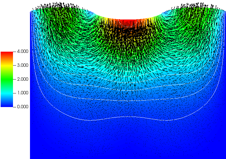
(a) Displacement $u$.

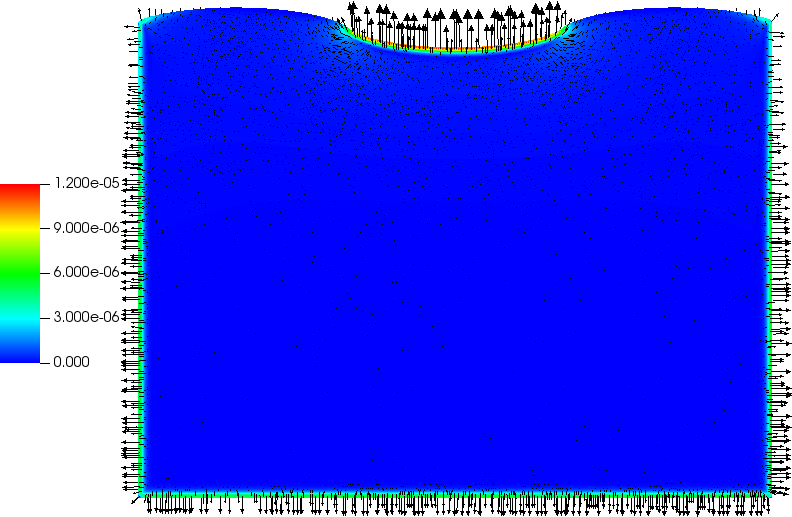
(b) Darcy velocity $z$.

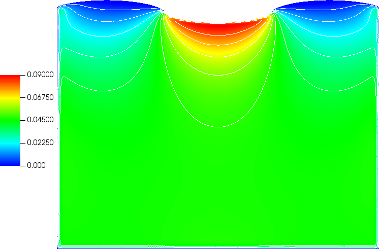
(c) Fluid pressure $p$.

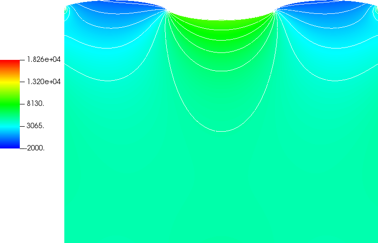
(d) Total pressure $p_{T}$.

Figure 1. The solution to the footing problem of section 5.3 in the deformed domain at $t=50$.

5.4. The cantilever bracket problem

The cantilever bracket problem was used in [2, 29, 32] to study locking phenomena at low permeability and when the storage coefficient is zero. Consider the domain $\Omega=(0,1)^{2}$ and define

$$\Gamma_{1} =\mathinner{\left\{(x_{1},x_{2})\in\partial\Omega,\ x_{2}=0\right\}}, \Gamma_{2} =\mathinner{\left\{(x_{1},x_{2})\in\partial\Omega,\ x_{1}=1\right\}},$$

$$\Gamma_{3} =\mathinner{\left\{(x_{1},x_{2})\in\partial\Omega,\ x_{2}=1\right\}}, \Gamma_{4} =\mathinner{\left\{(x_{1},x_{2})\in\partial\Omega,\ x_{1}=0\right\}}.$$

We impose the boundary conditions

$$z\cdot n=0\text{ on }\partial\Omega,\quad\sigma n=(0,-1)^{T}\text{ on }\Gamma_{3},\quad\sigma n=0\text{ on }\Gamma_{1}\cup\Gamma_{2},\quad u=0\text{ on }\Gamma_{4}.$$

At $t=0$ we set $u=0$ and $p=0$. The model parameters are chosen as $E=10^{5}$, $\nu=0.4$, $\alpha=0.93$, $c_{0}=0$, and $\kappa=10^{-7}$ [32]. As shown in [32], with these parameters continuous Galerkin numerical methods show spurious oscillations in the pressure on a very short time interval. Therefore, we consider here the time interval $I=[0,0.005]$. In our discretization we combine the EDG-HDG discretization with BDF2 time stepping, choose a time step of $\Delta t=0.001$, set $k=2$ in our finite element spaces, and compute the solution on a mesh consisting of 128 simplices.

We plot the solution in fig. 2. In fig. 2a we observe that the pressure field at $t=0.001$ is free from spurious oscillations, similar to the discontinuous Galerkin solutions obtained in [32]. We further show in fig. 2b that the pressure solution along the lines $x=0.26$, $x=0.33$, $x=0.4$, and $x=0.46$ at $t=0.005$ is free of oscillations, agreeing with other stable finite element methods for this problem [2, 29, 32].

(a) Pressure $p$ at $t=0.001$.

(b) Pressure $p$ along different $x$-lines.

Figure 2. The solution to the cantilever bracket problem section 5.4 using EDG-HDG. Left: the pressure solution at $t=0.001$. Right: the pressure solution along different $x$-lines at time $t=0.005$.

6. Conclusions

An HDG and an EDG-HDG method have been presented and analyzed for the total pressure formulation of the quasi-static poroelasticity model. Both discretization methods are shown to be well-posed and space-time a priori error estimates show robustness of the proposed methods when $\lambda\to\infty$ and $c_{0}\to 0$; both methods are free of volumetric locking. Numerical examples confirm our theory and further show optimal spatial rates of convergence in the $L^{2}$-norm.

Statements and Declarations

Funding For AC and JL this material is based upon work supported by the National Science Foundation under grant numbers DMS-2110782 and DMS-2110781. SR gratefully acknowledges support from the Natural Sciences and Engineering Research Council of Canada through the Discovery Grant program (RGPIN-05606-2015).

7. Appendix

7.1. The inf-sup condition for $b_{h}$

By definition of $b_{h}$ eq. 6b,

(48) $$b_{h}((w_{h},0),\bm{q}_{h})\mathrel{\mathop{\mathchar 58\relax}}=\underbrace{-(q_{h},\nabla\cdot w_{h})_{\Omega}}_{=\mathrel{\mathop{\mathchar 58\relax}}b_{h}^{1}(w_{h},q_{h})}+\underbrace{\langle\bar{q}_{h},w_{h}\cdot n\rangle_{\partial\mathcal{T}}}_{=\mathrel{\mathop{\mathchar 58\relax}}b_{h}^{2}(w_{h},\bar{q}_{h})}\quad\forall w_{h}\in V_{h},\forall\bm{q}_{h}\in\bm{Q}_{h}^{0}.$$

Let $q_{h}\in Q_{h}$. It is known (see, for example, [13, Section 4.1.4] or [27, Remark 3.3]) that there exists $w\in\mathinner{[H^{1}_{0,\Gamma_{F}}(\Omega)]}^{d}\mathrel{\mathop{\mathchar 58\relax}}=\mathinner{\{v\in\mathinner{[H^{1}(\Omega)]}^{d}\,\mathrel{\mathop{\mathchar 58\relax}}\,v|_{\Gamma_{F}}=0\}}$ such that

(49) $$-(\nabla\cdot w,q_{h})_{\Omega}=\|q_{h}\|_{\Omega}^{2},\quad\|w\|_{1,\Omega}\leq C\|q_{h}\|_{\Omega},$$

for some positive constant $C$ that only depends on $\Omega$. Let $\Pi_{V}\mathrel{\mathop{\mathchar 58\relax}}\mathinner{[H^{1}(\Omega)]}^{d}\rightarrow V_{h}$ be the BDM interpolation operator [8, Section III.3] and observe that by the single-valuedness of $\bar{q}_{h}$, continuity of $\Pi_{V}w\cdot n$ across interior faces, and since $\bar{q}_{h}=0$ on $\Gamma_{P}$ and $w=0$ on $\Gamma_{F}$,

$$b_{h}^{2}(\Pi_{V}w,\bar{q}_{h})=\langle\bar{q}_{h},\Pi_{V}w\cdot n\rangle_{\Gamma_{F}}=0,$$

i.e., $\Pi_{V}w\in\text{Ker}\,b_{2}\mathrel{\mathop{\mathchar 58\relax}}=\mathinner{\{w_{h}\in V_{h}\,\mathrel{\mathop{\mathchar 58\relax}}\,b_{h}^{2}(w_{h},\bar{q}_{h})=0\quad\forall\bar{q}_{h}\in\bar{Q}_{h}\}}$. Recall also that $(q_{h},\nabla\cdot\Pi_{V}w)_{\Omega}=(q_{h},\nabla\cdot w)_{\Omega}$ and $\|\Pi_{V}w\|_{\Omega}\leq C\|w\|_{1,\Omega}$. Then, by eq. 49,

$$\sup_{0\neq w_{h}\in\text{Ker}\,b_{2}}\frac{b_{h}^{1}(w_{h},q_{h})}{\|w_{h}\|_{\Omega}}\geq\frac{-(q_{h},\nabla\cdot\Pi_{V}w)_{\Omega}}{\|\Pi_{V}w\|_{\Omega}}\geq\frac{\|q_{h}\|^{2}_{\Omega}}{C\|q_{h}\|_{\Omega}}=C\|q_{h}\|_{\Omega}.$$

Next, let $w_{h}\mathrel{\mathop{\mathchar 58\relax}}=L\bar{q}_{h}\in P_{k}(K)^{d}$ where $L$ is the local BDM interpolation operator [8] such that

(50) $$(L\bar{q}_{h})\cdot n=\bar{q}_{h},\quad\|L\bar{q}_{h}\|_{K}\leq Ch_{K}^{1/2}\|\bar{q}_{h}\|_{\partial K},\quad K\in\mathcal{T}.$$

Then

$$\sup_{0\neq w_{h}\in V_{h}}\frac{b_{h}^{2}(w_{h},\bar{q}_{h})}{\|w_{h}\|_{\Omega}} \geq\frac{\|\bar{q}_{h}\|^{2}_{\partial\mathcal{T}}}{\|w_{h}\|_{\Omega}}\geq\frac{\|\bar{q}_{h}\|^{2}_{\partial\mathcal{T}}}{C\sum_{K\in\mathcal{T}}h_{K}^{-1}\|w_{h}\|_{\Omega}}$$

$$\geq Ch_{\min}h_{\max}^{-1}\Big{(}\sum_{K\in\mathcal{T}}h_{K}\|\bar{q}_{h}\|_{\partial K}^{2}\Big{)}^{1/2}.$$

Therefore, by [20, Theorem 3.1],

$$\sup_{0\neq w_{h}\in V_{h}}\frac{b_{h}((w_{h},0),\bm{q}_{h})}{\|w_{h}\|_{\Omega}} =\sup_{0\neq w_{h}\in V_{h}}\frac{b_{h}^{1}(w_{h},q_{h})+b_{h}^{2}(w_{h},\bar{q}_{h})}{\|w_{h}\|_{\Omega}}$$

$$\geq C\mathinner{\Bigl{(}\|q_{h}\|_{\Omega}+h_{\min}h_{\max}^{-1}\mathinner{\bigl{(}\sum_{K\in\mathcal{T}}h_{K}\|\bar{q}_{h}\|_{\partial K}^{2}\bigr{)}}\Bigr{)}}\geq C\mathopen{|\mkern-1.5mu|\mkern-1.5mu|}\bm{q}_{h}\mathclose{|\mkern-1.5mu|\mkern-1.5mu|}_{q}.$$

7.2. Error estimates following from Taylor’s theorem

We prove here eqs. 25a and 25b. Let $D\subset\mathbb{R}^{d}$. Then for $\psi$ a regular enough function defined on $[0,T]\times D$, using Taylor’s theorem,

$$\Delta t\|\partial_{t}\psi^{m}-d_{t}\psi^{m}\|_{0,D} =\|\Delta t\partial_{t}\psi^{m}-(\psi^{m}-\psi^{m-1})\|_{0,D}$$

$$=\|\int_{t_{m-1}}^{t_{m}}\partial_{tt}\psi(t)\underbrace{(t-t_{m-1})}_{\leq\Delta t}\operatorname{d\!}t\|_{0,D}$$

$$\leq\Delta t\int_{t_{m-1}}^{t_{m}}\|\partial_{tt}\psi(t)\|_{0,D}\operatorname{d\!}t$$

$$=\Delta t\|\partial_{tt}\psi\|_{L^{1}(t_{m-1},t_{m};L^{2}(D))},$$

from which eq. 25a follows. Next, to show eq. 25b we use the identity

$$\Delta td_{t}e_{\psi}^{I,m}=\int_{t^{m-1}}^{t^{m}}(\partial_{t}\psi(s)-\Pi_{Q}\partial_{t}\psi(s))\operatorname{d\!}s,$$

and eq. 20. Then, by the approximation property of the $L^{2}$-projection,

$$\begin{split}\Delta t\sum_{m=1}^{n}\|d_{t}e_{\psi}^{I,m}\|_{0,D}&\leq\sum_{m=1}^{n}\int_{t^{m-1}}^{t^{m}}\|\partial_{t}\psi(s)-\Pi_{Q}\partial_{t}\psi(s))\|_{0,D}\operatorname{d\!}s\\ &\leq Ch^{l}\|\partial_{t}\psi\|_{L^{1}(I;H^{l}(D))}.\end{split}$$

References

• [1] R.A. Adams, Sobolev spaces, Academic Press [A subsidiary of Harcourt Brace Jovanovich, Publishers], New York-London, 1975, Pure and Applied Mathematics, Vol. 65.
• [2] I. Ambartsumyan, E. Khattatov, and I. Yotov, A coupled multipoint stress–multipoint flux mixed finite element method for the Biot system of poroelasticity, Comput. Methods Appl. Mech. Engrg. 327 (2020), 113407.
• [3] D. N. Arnold and F. Brezzi, Mixed and nonconforming finite element methods: implementation, postprocessing and error estimates, RAIRO Modél. Math. Anal. Numér. 19 (1985), no. 1, 7–32.
• [4] M. A. Biot, Theory of propagation of elastic waves in a fluid-saturated porous solid. I. Low-frequency range, J. Acoust. Soc. Amer. 28 (1956), 168–178. MR 134056
• [5] by same author, Theory of propagation of elastic waves in a fluid-saturated porous solid. II. Higher frequency range, J. Acoust. Soc. Amer. 28 (1956), 179–191. MR 134057
• [6] Daniele Boffi, Michele Botti, and Daniele A. Di Pietro, A nonconforming high-order method for the Biot problem on general meshes, SIAM J. Sci. Comput. 38 (2016), no. 3, A1508–A1537. MR 3504993
• [7] Lorenzo Botti, Michele Botti, and Daniele A. Di Pietro, An abstract analysis framework for monolithic discretisations of poroelasticity with application to hybrid high-order methods, Comput. Math. Appl. 91 (2021), 150–175. MR 4253882
• [8] F. Brezzi and M. Fortin, Mixed and hybrid finite element methods, Springer Series in Computational Mathematics, vol. 15, Springer–Verlag New York Inc., 1991.
• [9] A. Cesmelioglu, S. Rhebergen, and G. N. Wells, An embedded-hybridized discontinuous Galerkin method for the coupled Stokes–Darcy system, Journal of Computational and Applied Mathematics 367 (2020), 112476.
• [10] B. Cockburn, J. Gopalakrishnan, and R. Lazarov, Unified hybridization of discontinuous Galerkin, mixed, and continuous Galerkin methods for second order elliptic problems, SIAM J Numer Anal 47 (2009), no. 2, 1319–1365.
• [11] B. Cockburn, J. Guzmán, S.-C. Soon, and H. K. Stolarski, An analysis of the embedded discontinuous Galerkin method for second-order elliptic problems, SIAM J. Numer. Anal. 47 (2009), no. 4, 2686–2707.
• [12] S. Du and F.-J. Sayas, An invitation to the theory of the hybridizable discontinuous Galerkin method: Projection, estimates, tools, SpringerBriefs Math., 2019.
• [13] A. Ern and J.-L. Guermond, Theory and practice of finite elements, Applied Mathematical Sciences, vol. 159, Springer–Verlag New York, 2004.
• [14] X. Feng, Z. Ge, and Y. Li, Analysis of a multiphysics finite element method for a poroelasticity model, IMA J. Numer. Anal. 38 (2018), no. 1, 330–359.
• [15] G. Fu, A high-order HDG method for the Biot’s consolidation model, Comput. Math. Appl. (2018).
• [16] F. J. Gaspar, F. J. Lisbona, and C. W. Oosterlee, A stabilized difference scheme for deformable porous media and its numerical resolution by multigrid methods, Comput. Visual Sci. 11 (2008), 67–76.
• [17] S. Güzey, B. Cockburn, and H. K. Stolarski, The embedded discontinuous Galerkin method: application to linear shell problems, International journal for numerical methods in engineering 70 (2007), no. 7, 757–790.
• [18] P. Hansbo and M. G. Larson, Discontinuous Galerkin methods for incompressible and nearly incompressible elasticity by Nitsche’s method, Comput. Methods Appl. Mech. Engrg. 191 (2002), 1895–1908.
• [19] Qingguo Hong and Johannes Kraus, Parameter-robust stability of classical three-field formulation of Biot’s consolidation model, Electron. Trans. Numer. Anal. 48 (2018), 202–226. MR 3820123
• [20] J. S. Howell and N. J. Walkington, Inf-sup conditions for twofold saddle point problems, Numer. Math. 118 (2011), 663–693.
• [21] Xiaozhe Hu, Carmen Rodrigo, Francisco J. Gaspar, and Ludmil T. Zikatanov, A nonconforming finite element method for the Biot’s consolidation model in poroelasticity, J. Comput. Appl. Math. 310 (2017), 143–154. MR 3544596
• [22] G. Kanschat and B. Rivière, A finite element method with strong mass conservation for Biot’s linear consolidation model, J. Sci. Comput. (2018).
• [23] R. F. Katz, M. G. Knepley, B. Smith, M. Spiegelman, and E. T. Coon, Numerical simulation of geodynamic processes with the portable extensible toolkit for scientific computation, Phys. Earth Planet. In. 163 (2007), no. 1–4, 52–68.
• [24] T. Keller, D. A. May, and B. J. P. Kaus, Numerical modelling of magma dynamics coupled to tectonic deformation of lithosphere and crust, Geophys. J. Int. 195 (2013), 1406–1442.
• [25] Johannes Kraus, Philip L. Lederer, Maria Lymbery, and Joachim Schöberl, Uniformly well-posed hybridized discontinuous Galerkin/hybrid mixed discretizations for Biot’s consolidation model, Comput. Methods Appl. Mech. Engrg. 384 (2021), Paper No. 113991, 23. MR 4274934
• [26] J. J. Lee, Robust error analysis of coupled mixed methods for Biot’s consolidation model, Journal of Scientific Computing 69 (2016), no. 2, 610–632.
• [27] J. J. Lee, K. Mardal, and R. Winther, Parameter-robust discretization and preconditioning of Biot’s consolidation model, SIAM Journal on Scientific Computing 39 (2017), no. 1, A1–A24.
• [28] Jeonghun J. Lee, Robust three-field finite element methods for Biot’s consolidation model in poroelasticity, BIT (2017).
• [29] R. Liu, Discontinuous Galerkin finite element solution for poromechanics, Ph.D. thesis, The University of Texas at Austin, 2004.
• [30] Márcio A Murad, Vidar Thomée, and Abimael FD Loula, Asymptotic behavior of semidiscrete finite-element approximations of Biot’s consolidation problem, SIAM J. Numer. Anal. 33 (1996), no. 3, 1065–1083.
• [31] R. Oyarzúa and R. Ruiz-Baier, Locking-free finite element methods for poroelasticity, SIAM J. Numer. Anal. 54 (2016), no. 5, 2951–2973.
• [32] P. J. Phillips and M. F. Wheeler, Overcoming the problem of locking in linear elasticity and poroelasticity: an heuristic approach, Computat. Geosci. 13 (2009), 5–12.
• [33] Phillip Joseph Phillips and Mary F. Wheeler, A coupling of mixed and discontinuous Galerkin finite-element methods for poroelasticity, Comput. Geosci. 12 (2008), no. 4, 417–435. MR 2461315
• [34] S. Rhebergen and G. Wells, Analysis of a hybridized/interface stabilized finite element method for the Stokes equations, SIAM J. Numer. Anal. 55 (2017), no. 4, 1982–2003.
• [35] S. Rhebergen and G. N. Wells, Preconditioning of a hybridized discontinuous Galerkin finite element method for the Stokes equations, J. Sci. Comput. (2018).
• [36] by same author, An embedded-hybridized discontinuous Galerkin finite element method for the Stokes equations, Comput. Methods Appl. Mech. Engrg. 358 (2020).
• [37] B. Rivière, Jun Tan, and Travis Thompson, Error analysis of primal discontinuous Galerkin methods for a mixed formulation of the Biot equations, Comput. Math. Appl. 73 (2017), no. 4, 666 – 683.
• [38] C. Rodrigo, F. J. Gaspar, X. Hu, and L. T. Zikatanov, Stability and monotonicity for some discretizations of the Biot’s consolidation model, Comput. Methods Appl. Mech. Engrg. 298 (2016), 183–204. MR 3427711
• [39] Juan Enrique Santos, Elastic wave propagation in fluid-saturated porous media. I. The existence and uniqueness theorems, RAIRO Modél. Math. Anal. Numér. 20 (1986), no. 1, 113–128. MR 844519
• [40] Juan Enrique Santos and Ernesto Jorge Oreña, Elastic wave propagation in fluid-saturated porous media. II. The Galerkin procedures, RAIRO Modél. Math. Anal. Numér. 20 (1986), no. 1, 129–139. MR 844520
• [41] J. Schöberl, An advancing front 2D/3D-mesh generator based on abstract rules, J. Comput. Visual Sci. 1 (1997), no. 1, 41–52.
• [42] by same author, C++11 implementation of finite elements in NGSolve, Tech. Report ASC Report 30/2014, Institute for Analysis and Scientific Computing, Vienna University of Technology, 2014.
• [43] R. E. Showalter, Diffusion in poro-elastic media, J. Math. Anal. Appl. 251 (2000), no. 1, 310–340. MR 1790411
• [44] Alexander Ženíšek, The existence and uniqueness theorem in Biot’s consolidation theory, Apl. Mat. 29 (1984), no. 3, 194–211. MR 747212
• [45] G. N. Wells, Analysis of an interface stabilized finite element method: the advection-diffusion-reaction equation, SIAM J. Numer. Anal. 49 (2011), no. 1, 87–109.
• [46] S.-Y. Yi, A coupling of nonconforming and mixed finite element methods for Biot’s consolidation model, Numer. Meth. Part. D. E. 29 (2013), no. 5, 1749–1777.
• [47] Son-Young Yi, Convergence analysis of a new mixed finite element method for Biot’s consolidation model, Numer. Methods Partial Differential Equations 30 (2014), no. 4, 1189–1210. MR 3200272
• [48] by same author, A study of two modes of locking in poroelasticity, SIAM J. Numer. Anal. 55 (2017), no. 4, 1915–1936.
• [49] O. C. Zienkiewicz and T. Shiomi, Dynamic behaviour of saturated porous media; the generalized Biot formulation and its numerical solution, International Journal for Numerical and Analytical Methods in Geomechanics 8 (1984), no. 1, 71–96.