A Three-phase Power Flow Model and Balanced Network Analysis

Abstract

First we present an approach to formulate unbalanced three-phase power flow problems for general networks that explicitly separates device models and network models. A device model consists of (i) an internal model and (ii) a conversion rule. The conversion rule relates the internal variables (voltage, current, and power) of a device to its terminal variables through a conversion matrix $\Gamma$ and these terminal variables are related by network equations. Second we apply this approach to balanced three-phase networks to formalize per-phase analysis and prove its validity for general networks using the spectral property of the conversion matrix $\Gamma$.

I Introduction

Motivation. Unbalanced three-phase load flow problems are becoming increasingly important as we decarbonize the grid. Such problems are more difficult for several reasons; see, e.g., [1, Chapter 11] for transmission systems and [2] for distribution systems. First, a network model is more complicated because three-phase lines couple currents and voltages in different phases when lines are not transposed or loads are unbalanced, e.g., as in most distribution systems. If the network is symmetric, then a similarity transformation due to Fortescue [3] from the phase coordinate to a sequence coordinate produces network models that are decoupled in the sequence coordinate and can therefore be analyzed in a way similar to a single-phase network; see, e.g., [4]. Without symmetry, this transformation however offers no simplification. Second, the voltages and currents across the single-phase devices internal to $\Delta$ configuration are observed externally only through a linear map $\Gamma$ that is not invertible. While we are typically interested in solving for or optimizing the internal currents or power flows across the single-phase devices, e.g., controlling the charging currents of electric vehicle chargers in $\Delta$ configuration, a network model, such as $I=YV$ or $s_{j}=\sum_{k}y_{jk}^{s}\left(|V_{j}|^{2}-V_{j}V_{k}^{\sf H}\right)$, relates only the terminal voltages and currents observable externally of three-phase devices. The interplay between internal and external variables of a three-phase device sometimes seems confusing. Third, load flow formulations sometimes implicitly assume that the neutrals of all $Y$-configured devices are at zero potential and the zero-sequence components of the terminal voltages of all $\Delta$-configured devices are zero. This limits their applicability as, e.g., they exclude the case where some $Y$-configured loads are ungrounded or grounded with nonzero earthing imepdances. Solutions to the last two difficulties both lie in a careful accounting of the conversion between internal and external variables of $\Delta$-configured devices, using the conversion matrix $\Gamma$.

Summary. In this paper we present such a modeling approach that separates three-phase device models and network networks. In this approach, a device model consists of two components: (i) an internal model and (ii) a conversion rule. The internal model describes how each of the single-phase device behaves regardless of their configuration. The conversion rule, on the other hand, depends only on their configuration regardless of the type of devices. It maps internal voltages, currents, and powers across these single-phase devices to terminal voltages, currents, and powers observable externally. Since the network model relates only the terminal variables regardless of the type of devices or their configurations, the explicit separation of device and network models allows mix and match of equivalent models, enhancing modeling flexibility. We present our model in Section II and use it to formulate an unbalanced three-phase analysis problem for general networks in Section III.

In Section IV we illustrate our model by showing formally that the analysis problem can be solved using per-phase analysis when the network is balanced. It is well known that a balanced three-phase device in $\Delta$ configuration has an $Y$ equivalent that has the same external behavior. The standard way to justify per-phase analysis is by analyzing specific three-phase circuits, often simple circuits; e.g., [5, 6, 7], by first converting all $\Delta$-configured devices into their $Y$ equivalents, and then showing that all neutrals in the equivalent circuit are at the same potential and that all phases are decoupled. This implies that the original three-phase circuit can be solved by analyzing a simpler per-phase circuit. This process has two limitations.

First, it is not clear how to extend circuit analysis methods, e.g., loop analysis or mesh analysis [5, Chapter 12], from specific (and simple) circuits to an arbitrary balanced network and prove that all neutrals are at the same potential. This is simple to show, however, in our model by expressing the network equation $I=YV$ in terms of the Kronecker product and using the spectral property of $\Gamma$ (see Theorems 2 and 3). The intuition is as follows. In a balanced three-phase network, positive-sequence voltages and currents are in span$(\alpha_{+})$ where $\alpha_{+}$ is an eigenvector of $\Gamma$ and $\Gamma^{\sf T}$. This means that the transformation of balanced voltages and currents under $\left(\Gamma,\Gamma^{\sf T}\right)$ reduces to a scaling of these variables by their eigenvalues $1-\alpha$ and $1-\alpha^{2}$ respectively. The voltage and current at every point in a network can be written as linear combinations of transformed source voltages and source currents, transformed by $\left(\Gamma,\Gamma^{\sf T}\right)$ and line admittance matrices. Therefore if the source voltages and source currents are in span$(\alpha_{+})$ and if lines are identical and phase-decoupled, then the transformed voltages and currents remain in span$(\alpha_{+})$ and hence are balanced positive-sequence sets. This is explained in Sections IV-B, IV-C and IV-E.

Second, all neutrals are at the same potential only if the neutral voltages of all $Y$-configured devices (voltage sources, current sources and impedances) are assumed zero and the zero-sequence voltages of all $\Delta$-configured voltage sources are assumed zero. Roughly, this requires that all neutrals are grounded directly (i.e., with zero earthing impedances). The standard analysis of specific circuits often makes this assumption sometimes implicitly. Without this assumption, the neutral voltages on the circuit are generally different. Yet, per-phase analysis can be extended to the general case without this assumption as long as the network is balanced, except that per-phase analysis is needed not only on a per-phase positive-sequence network, but also on a per-phase zero-sequence network. This is explained in Section IV-D.

We close our summary with two remarks on per-phase analysis. First, if the network is unbalanced but symmetric, i.e., impedances are balanced and lines are (phase coupled but) symmetric, then Fortescue’s similarity transformation [3] from the phase coordinate to the sequence coordinate leads to decoupled device models and network models. The network equation is therefore decoupled in the sequence coordinate and can be interpreted as defining three separate sequence networks, to which the per-phase analysis of Section IV can be applied. Second, with today’s abundant computing power the smaller problem size may not be an important advantage of per-phase analysis. Rather, per-phase analysis illustrates the application of our modeling approach to three-phase power flow. It also clarifies the simple structure underlying a balanced network and enhances our conceptual understanding of three-phase networks in general, balanced or unbalanced.

Literature. Single-phase models are a good approximation for many transmission network applications where lines are symmetric and loads are balanced so that the zero and negative-sequence components are negligible compared with the positive-sequence component. They may not be negligible when lines are not transposed or equally spaced, e.g., as in distribution systems, and when loads are unbalanced or nonlinear, e.g., AC furnaces, high-speed trains, power electronics, or single or two-phase laterals in distribution networks. This can cause power quality issues such as voltage imbalances and harmonics. Furthermore single-phase analysis can produce incorrect power flow solutions.

There is a large literature on three-phase power flow analysis and we only make a few brief remarks. Three-phase load flow solvers have been developed since at least the 1960s, e.g., see [8] for solution in the sequence coordinate and [9, 10] in the phase coordinate. A three-phase network is equivalent to a single-phase circuit where each node in the equivalent circuit is indexed by a (bus, phase) pair [10]. Single-phase power flow algorithms such as Newton Raphson [11] or Fast Decoupled methods [12] can be directly applied to the equivalent circuit. The main difference with a single-phase network is the circuit models of three-phase devices in the equivalent circuit, such as models for three-phase lines [13, 2], transformers and co-generators [10, 14], constant-power devices [1, Chapter 11], as well as voltage regulators, and loads [2], etc. A state-of-the-art algorithm in [1, Chapter 11] expresses currents in terms of voltages for both $PQ$ and $PV$ buses, applies the Newton-Raphson algorithm to the resulting nonlinear current balance equation $I=YV$ in the sequence domain. It allows both grounded and ungrounded loads in $Y$ and $\Delta$ configurations. For transmission networks, computing in the sequence domain has the advantage that, when most lines in the network are symmetric and thus have decoupled representation in the sequence coordinate, the Jacobian matrix is sparse. Sometimes an approximate solution is computed by ignoring the coupling across zero, positive, and negative-sequence variables and solving the three sequence networks separately as single-phase networks, e.g., [15]. Distribution networks usually does not enjoy such simplification and hence computation is usually done in the phase coordinate.

While the papers above study general networks that may contain cycles, another set of power flow methods are tailored for three-phase radial networks [9, 16, 2, 17, 18, 19]. In particular, the tree topology leads to a spatially recursive structure that enables iterative algorithms called backward forward sweep (BFS), apparently first developed in [9]. Different BFS algorithms are developed in [16][2, Chapter 10.1.3] [17] for three-phase networks ([17] generalizing the BFS algorithm of [20] from single-phase to three-phase networks). For single-phase radial networks, a solution method based on the DistFlow model is developed in [21] that uses one-time forward sweep (to express all variables in terms of the voltages at the feeder head and all branch points) followed by a Newton-Raphson algorithm to solve for these voltages. By exploiting the approximate sparsity of the Jacobian matrix in [21], approximate fast decoupled methods are developed and their convergence properties analyzed in [22]. These methods are extended to three-phase radial networks in [18]. The existence and uniqueness of power flow solutions of three-phase DistFlow model is analyzed in [19]. The advantage of BFS is that it does not need to compute Jacobian nor solve a linear system to compute iteration updates. Newton-Raphson, on the other hand, tends to converge in a smaller number of iterations.

Notation. Let $\mathbb{C}$ denote the set of complex numbers. For $a\in\mathbb{C}$, Re$\,\,a$ and Im$\,\,a$ denote its real and imaginary parts respectively, and $\bar{a}$ or $a^{\sf H}$ denotes its complex conjugate. We use $\mathbf{i}$ to denote $\sqrt{-1}$. A vector $x\in\mathbb{C}^{n}$ is a column vector and is denoted in one of two ways:

$$x \ \ =\ \ \begin{bmatrix}x_{1}\\ \vdots\\ x_{n}\end{bmatrix}, x \ \ =\ \ (x_{1},\dots,x_{n})$$

Its componentwise complex conjugate is denoted by $\overline{x}$. For any matrix $A$, $A^{\sf T}$, $A^{\sf H}$, $A^{\dagger}$ denote its transpose, Hermitian transpose, and pseudo-inverse respectively. If $x$ is a matrix then $\mathrm{diag}\left(x\right)$ is the vector whose components are the diagonal entries of $x$, whereas if $x$ is a vector then $\mathrm{diag}(x)$ is a diagonal matrix with $x_{i}$ as its diagonal entries. Finally $\textbf{1}\in\mathbb{C}^{3}$ is the column vector of size 3 whose entries are all 1s and $\mathbb{I}$ is the identity matrix of size 3.

II Three-phase network model

A three-phase network connects generators to loads, each of which is modeled by a single-terminal device. Each terminal has three wires (or ports or conductors) indexed by its phases $a,b,c$, and possibly a neutral wire indexed by $n$. Internally, the device can be in $Y$ or $\Delta$ configuration, and the $Y$ configuration may have a neutral wire that may be grounded. A three-phase line has two terminals, each terminal with three or four wires, and it connects two single-terminal devices, one at each end of the line. Its neutral wire may be grounded at regular spacing along the line. The overall network model consists of three components (see Figure 1):

1. Device model. The internal behavior of a single-terminal device is defined by the relationship between the voltages $V^{Y}/V^{\Delta}$, currents $I^{Y}/I^{\Delta}$, and powers $s^{Y}/s^{\Delta}$ across each of the single-phase devices that make up the three-phase device. This relationship is independent of whether the device is in $Y$ or $\Delta$ configuration. The configuration defines a conversion rule that maps internal variables $\left(V^{Y/\Delta},I^{Y/\Delta},s^{Y/\Delta}\right)\in\mathbb{C}^{9}$ to terminal voltages, currents, and powers $(V,I,s)\in\mathbb{C}^{9}$, regardless of the type of the devices. The internal behavior and the conversion rule jointly determine the external behavior of the three-phase device, i.e., the relationship between the terminal variables $(V,I,s)$ that can be observed externally.

2. Line model. It relates the terminal voltages, line currents, and line power flows $(V_{j},I_{jk},S_{jk})\in\mathbb{C}^{9}$ and $(V_{k},I_{kj},S_{kj})\in\mathbb{C}^{9}$, at each end of the line $(j,k)$.

3. Network model. It relates the terminal variables of all devices on the network. This is defined by current or power balance at every bus in the network.

Figure 1: Overall three-phase network model.

In this section we present circuit models of four types of single-terminal devices, a voltage source, a current source, a power source, and an impedance. Then we present a circuit model of a three-phase line. Finally we compose an overall model of a network of such devices.

II-A Conversion matrices $\Gamma,\Gamma^{\sf T}$

We start by defining conversion matrices $\Gamma,\Gamma^{\sf T}$ that maps between internal and external variables in a $\Delta$ configuration:

$$\Gamma := \begin{bmatrix}1&-1&0\\ 0&1&-1\\ -1&0&1\end{bmatrix}$$ (1a)

$$\Gamma^{\sf T} := \begin{bmatrix}1&0&-1\\ -1&1&0\\ 0&-1&1\end{bmatrix}$$ (1b)

As we will see,

the spectral properties of $\Gamma,\Gamma^{\sf T}$ underlie much of the behavior of three-phase systems, balanced or unbalanced. Here we recall some basic facts on $\Gamma,\Gamma^{\sf T}$ that are useful in the rest of the paper.

It can be shown that $\Gamma$ and $\Gamma^{\sf T}$ are normal matrices and their spectral decompositions are

$$\Gamma \ \ =\ \ F\Lambda\overline{F},\qquad\qquad\Gamma^{\sf T}\ \ =\ \ \overline{F}\Lambda F$$

where $\Lambda$ is a diagonal matrix and $F$ is a unitary matrix defined as:

$$\Lambda \ \ :=\ \ \begin{bmatrix}0&&\\ &1-\alpha&\\ &&1-\alpha^{2}\end{bmatrix}, F \ \ :=\ \ \frac{1}{\sqrt{3}}\begin{bmatrix}\textbf{1}&\alpha_{+}&\alpha_{-}\end{bmatrix}$$ (2)

with $\alpha:=e^{-\mathbf{i}2\pi/3}$. The positive-sequence and negative-sequence vectors $\left(\alpha_{+},\alpha_{-}\right)$ are

$$\alpha_{+} := \begin{bmatrix}1\\ \alpha\\ \alpha^{2}\end{bmatrix},\qquad\qquad\alpha_{-}\ \ :=\ \ \begin{bmatrix}1\\ \alpha^{2}\\ \alpha\end{bmatrix}$$

The eigenvectors of $\Gamma$ are $\textbf{1},\alpha_{+},\alpha_{-}$ and they are orthogonal. Here $\overline{F}$ is the complex conjugate of $F$ componentwise. Since $F$ is symmetric, the pseudo inverses of $\Gamma,\Gamma^{\sf T}$ are

$$\Gamma^{\dagger} \ \ =\ \ F\Lambda^{\dagger}\overline{F},\qquad\qquad\Gamma^{\sf T{\dagger}}\ \ =\ \ \overline{F}\Lambda^{\dagger}F$$

where $\Lambda^{\dagger}:=\mathrm{diag}\left(0,(1-\alpha)^{-1},(1-\alpha^{2})^{-1}\right)$. This yields the following properties.

Lemma 1 (Pseudo inverses of $\Gamma,\Gamma^{\sf T}$).

1. The null spaces of $\Gamma$ and $\Gamma^{\sf T}$ are both span$(\textbf{1})$.

2. Their pseudo-inverses are

   $$\Gamma^{\dagger}\ \ =\ \ \frac{1}{3}\,\Gamma^{\sf T},\qquad\quad\Gamma^{\sf T{\dagger}}\ \ =\ \ \frac{1}{3}\,\Gamma$$

3. Consider $\Gamma x=b$ where $b,x\in\mathbb{C}^{3}$. Solutions $x$ exist if and only if $\textbf{1}^{\sf T}b=0$, in which case the solutions $x$ are given by

   $$x = \frac{1}{3}\,\Gamma^{\sf T}b\ +\ \gamma\textbf{1},\qquad\qquad\gamma\in\mathbb{C}$$

4. Consider $\Gamma^{\sf T}x=b$ where $b,x\in\mathbb{C}^{3}$. Solutions $x$ exist if and only if $\textbf{1}^{\sf T}b=0$, in which case the solutions $x$ are given by

   $$x = \frac{1}{3}\,\Gamma b\ +\ \gamma\textbf{1},\qquad\qquad\gamma\in\mathbb{C}$$

5. $\Gamma\Gamma^{\dagger}=\Gamma^{\dagger}\Gamma=\frac{1}{3}\,\Gamma\Gamma^{\sf T}\ =\ \frac{1}{3}\,\Gamma^{\sf T}\Gamma\ \ =\ \ \mathbb{I}\ -\ \frac{1}{3}\,\textbf{1}\textbf{1}^{\sf T}$ where $\mathbb{I}$ is the identity matrix of size 3.

In this paper, we will use Lemma 1 repeatedly, sometimes without explicit reference.

II-B Devices: internal models and conversion rules

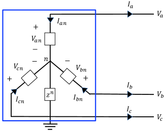
(a) $Y$ configuration

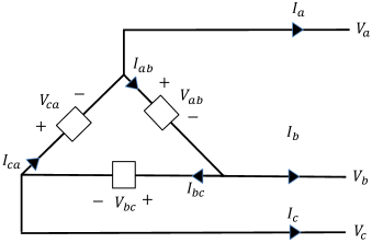
(b) $\Delta$ configuration

Figure 2: Internal and external variables associated with a single-terminal device in $Y$ and $\Delta$ configurations. (Even though Figure 2(a) shows a grounded device, our model allows each $Y$-configured device to be grounded or ungrounded and, if grounded, $z^{n}$ to be zero or nonzero.)

The internal behavior of a single-terminal device shown in Figure 2 is described in terms of its internal variables:

• $V^{Y}:=\left(V^{an},V^{bn},V^{cn}\right)\in\mathbb{C}^{3}$, $I^{Y}:=\left(I^{an},I^{bn},I^{cn}\right)\in\mathbb{C}^{3}$, $s^{Y}:=\left(s^{an},s^{bn},s^{cn}\right)\in\mathbb{C}^{3}$ : line-to-neutral voltages, currents, and power across the single-phase devices in $Y$ configuration. By definition $s^{an}:=V^{an}\left(I^{an}\right)^{\sf H}$ is the power across the phase-$a$ device, etc. The neutral voltage (with respect to a common reference point) is denoted by $V^{n}$ and is generally nonzero. A $Y$-configured device may or may not have a neutral line which may or may not be grounded (Figure 2 shows the case where the device is grounded through an impedance $z^{n}$). When present, the current on the neutral line is denoted by $I^{n}$ in the direction away from the neutral.

• $V^{\Delta}:=\left(V^{ab},V^{bc},V^{ca}\right)\in\mathbb{C}^{3}$, $I^{\Delta}:=\left(I^{ab},I^{bc},I^{ca}\right)\in\mathbb{C}^{3}$, $s^{\Delta}:=\left(s^{ab},s^{bc},s^{ca}\right)\in\mathbb{C}^{3}$ : line-to-line voltages, currents, and power across the single-phase devices in $\Delta$ configuration. By definition $s^{ab}:=V^{ab}\left(I^{ab}\right)^{\sf H}$ is the power across the phase-$a$ device, etc.

Note that the direction of power $s^{an}$ or $s^{ab}$ across a single-phase device is defined in the direction of the current through the device.

Internal models.

The internal behavior of a three-phase device is described by the relation between the internal variables $\left(V^{Y},I^{Y},s^{Y}\right)$ or between $\left(V^{\Delta},I^{\Delta},s^{\Delta}\right)$. It depends on the property of the single-phase device, but not on their configuration nor the presence of a neutral line:

1. Voltage source: An ideal voltage source fixes the internal voltage $V^{Y/\Delta}$ to be a given constant $E^{Y/\Delta}$.

2. Current source: An ideal current source fixes the internal current $I^{Y/\Delta}$ to be a given constant $J^{Y/\Delta}$.

3. Power Source: An ideal power source fixes the internal power $s^{Y/\Delta}$ to be a given constant $\sigma^{Y/\Delta}$.

4. Impedance: An impedance $z^{Y/\Delta}$ is a $3\times 3$ complex matrix. It fixes the relationship between its internal variables to be:

   $$V^{Y/\Delta} \ \ =\ \ z^{Y/\Delta}\,I^{Y/\Delta}, s^{Y/\Delta} \ \ :=\ \ \mathrm{diag}\left(V^{Y/\Delta}\left(I^{Y/\Delta}\right)^{\sf H}\right)$$

The voltage and current $\left(V^{Y/\Delta},I^{Y/\Delta}\right)$ of a power source $\sigma^{Y/\Delta}$ are related quadratically by

$$\sigma^{Y/\Delta} \ \ =\ \ \mathrm{diag}\left(V^{Y/\Delta}\left(I^{Y/\Delta}\right)^{\sf H}\right)$$

The specification as well as internal and external variables of a three-phase device are summarized in Table I.

	Voltage	Current	Power	Impedances
Device specification	$E^{Y/\Delta}$	$J^{Y/\Delta}$	$\sigma^{Y/\Delta}$	$z^{Y/\Delta}$, $y^{Y/\Delta}$, $z^{n}$
Internal variables	$V^{Y/\Delta}$	$I^{Y/\Delta}$	$s^{Y/\Delta}$
External variables	$V$	$I$	$s$

TABLE I: Notation for three-phase single-terminal devices $(y^{Y/\Delta}:=\left(z^{Y/\Delta}\right)^{-1})$.

As noted above, the internal model does not depend on the configuration nor the presence of a neutral line.

Conversion rules.

The external behavior of the single-terminal device shown in Figure 2 is described in terms of its terminal variables:

• $V:=\left(V^{a},V^{b},V^{c}\right)\in\mathbb{C}^{3}$, $I:=\left(I^{a},I^{b},I^{c}\right)\in\mathbb{C}^{3}$, $s:=\left(s^{a},s^{b},s^{c}\right)\in\mathbb{C}^{3}$ : terminal voltages, currents, and power. The terminal voltage $V$ is defined with respect to an arbitrary but common reference point, e.g., the ground. The terminal current $I$ is defined in the direction coming out of the device, i.e., $I$ is defined to be the current injection from the device to the rest of the network when it is connected to a bus bar, regardless of whether it generates or consumes power. By definition $s^{a}:=V^{a}\,I^{a\sf H}$ is the power across terminal $a$ and the common reference point, etc.

The external model of a device is the relationship between its terminal variables $(V,I,s)$. We now derive the conversion rules (3) and (II-B) that maps internal variables $\left(V^{Y/\Delta},I^{Y/\Delta},s^{Y/\Delta}\right)$ to external variables $(V,I,s)$ for devices in $Y$ and $\Delta$ configurations respectively. These conversion rules depend only on the configuration and not on the type of devices. In Section II-C, we apply these conversion rules to the internal model of each device to derive its external model.

Conversion in $Y$ configuration. The terminal voltage, current, and power $(V,I,s)$ of a $Y$-configured device are related to the internal variables $(V^{Y},I^{Y},s^{Y})$ by:

$$V \ =\ V^{Y}\ +\ V^{n}\textbf{1}, I \ =\ -I^{Y}, s \ =\ -\left(s^{Y}\ +\ V^{n}\overline{I}^{Y}\right)$$ (3)

where $\overline{I}$ denotes the componentwise complex conjugate of the vector $I^{Y}\in\mathbb{C}^{3}$. The negative sign on the current and power conversions is due to the definition of $\left(I^{Y},s^{Y}\right)$ as internal current and power delivered to the single-phase devices whereas $(I,s)$ is defined as the terminal current and power injections out of the three-phase device.

In general the neutral voltage $V^{n}$ with respect to a common reference point is nonzero whether or not there is a neutral line and whether or not the neutral is grounded. If the neutral is grounded with zero neutral impedance and voltages are defined with respect to the ground, then $V^{n}=0$ and $V=V^{Y}$ and $s=-s^{Y}$. It is important to explicitly include $V^{n}$ in a network model because not every device in a network may be grounded or grounded with zero neutral impedance.

Remark 1 (Total power).

The total terminal power is

$$\textbf{1}^{\sf T}s \ \ =\ \ -\textbf{1}^{\sf T}s^{Y}\ -\ V^{n}\left(\textbf{1}^{T}\overline{I}^{Y}\right)$$

The first term $\textbf{1}^{\sf T}s^{Y}$ is the total power delivered across the single-phase devices. The second term $\textbf{1}^{T}I^{Y}$ is the sum of internal line-to-neutral current. If the neutral is grounded through an impedance then $V^{n}\left(\textbf{1}^{T}\overline{I}^{Y}\right)$ is the power delivered to the neutral impedance. If the neutral is ungrounded then $\textbf{1}^{T}I^{Y}=0$ by KCL and the second term $V^{n}\left(\textbf{1}^{T}\overline{I}^{Y}\right)=0$. ∎

Conversion in $\Delta$ configuration. The relationship between terminal voltage and current $(V,I)$ and internal voltage and current $\left(V^{\Delta},I^{\Delta}\right)$ is:

$$V^{\Delta} \ \ =\ \ \Gamma\,V,\qquad\quad I\ \ =\ \ -\Gamma^{\sf T}\,I^{\Delta}$$ (4a)

Given appropriate vectors $$V^{\Delta} I V I^{\Delta}$$ and , solutions and to (4a) is provided by Lemma 1.

1. Given $V^{\Delta}$, there is a solution $V$ to (4a) if and only if $V^{\Delta}$ is orthogonal to 1, i.e.,

   $$V^{ab}+V^{bc}+V^{ca} = 0$$

   which expresses Kirchhoff’s voltage law. In that case, there is a subspace of solutions $V$ given by

   $$V = \frac{1}{3}\,\Gamma^{\sf T}V^{\Delta}\ +\ \gamma\,\textbf{1},\quad\gamma\in\mathbb{\mathbb{missing}}C$$ (4b)

   This amounts to an arbitrary reference voltage for $V$. The quantity $\gamma:=\frac{1}{3}\textbf{1}^{\sf T}V$ is the (scaled) zero-sequence voltage of $V$. In most applications we are given a reference voltage (e.g., $V_{0}:=\alpha_{+}$ at the reference bus 0) which will fix the constant $\gamma$.

2. Given $I$, there is a solution $I^{\Delta}$ to (4a) if and only if $I$ is orthogonal to 1, i.e.,

   $$I^{a}+I^{b}+I^{c} = 0$$

   which expresses Kirchhoff’s current law. In that case, there is a subspace of $I^{\Delta}$ that satisfy (4a), given by

   $$I^{\Delta} = -\frac{1}{3}\,\Gamma I\ +\ \beta\,\textbf{1},\quad\beta\in\mathbb{C}$$ (4c)

   where $\beta$ specifies the amount of loop flow in $I^{\Delta}$ and does not affect the terminal current $I$ since $\Gamma^{\sf T}\beta\textbf{1}=0$. The quantity $\beta:=\frac{1}{3}\textbf{1}^{\sf T}I^{\Delta}$ is the (scaled) zero-sequence current of $I^{\Delta}$.

The terminal power injection from the device is $s:=\mathrm{diag}\left(VI^{\sf H}\right)$ and the internal power delivered across the single-phase devices in the direction $ab$, $bc$, $ca$ is $s^{\Delta}:=\mathrm{diag}\left(V^{\Delta}I^{\Delta\sf H}\right)$. Given internal voltage and current $\left(V^{\Delta},I^{\Delta}\right)$ with $\textbf{1}^{\sf T}V^{\Delta}=0$, the terminal power $s$ is (from (4a) (4b)):

$$s \ =\ -\mathrm{diag}\left(\Gamma^{\dagger}\left(V^{\Delta}I^{\Delta\sf H}\right)\Gamma\right)+\,\gamma\overline{I}, \textbf{1}^{\sf T}V^{\Delta} \ =\ 0$$ (4d)

where $\overline{I}$ is the complex conjugate of the terminal current $I=-\Gamma^{\sf T}I^{\Delta}$ and $\gamma\in\mathbb{C}$ is determined by a reference voltage. Conversely, given terminal voltage and current $(V,I)$ with $\textbf{1}^{\sf T}I=0$, the internal power $s^{\Delta}$ is (from (4a) (4c)):

$$s^{\Delta} \ =\-\mathrm{diag}\left(\Gamma\left(VI^{\sf H}\right)\Gamma^{\dagger}\right)+\,\beta V^{\Delta}, \textbf{1}^{\sf T}I \ =\ 0$$ (4e)

where $V^{\Delta}=\Gamma V$ and $\beta\in\mathbb{C}$ is determined by the zero-sequence current of $I^{\Delta}$.

Remark 2 (Total power).

1. Given an internal voltage and current $\left(V^{\Delta},I^{\Delta}\right)$, the terminal power vector $s$ does not depend on the zero-sequence current $\beta:=\frac{1}{3}\textbf{1}^{\sf T}I^{\Delta}$ but does depend on the zero-sequence voltage $\gamma:=\frac{1}{3}\textbf{1}^{\sf T}V$. Since $I=-\Gamma^{\sf T}I^{\Delta}$ and hence $\textbf{1}^{\sf T}I=0$, the total terminal power however is independent of $\gamma$:

   $$\textbf{1}^{\sf T}\,s \ \ =\ \ -\textbf{1}^{\sf T}\mathrm{diag}\left(\Gamma^{\dagger}\left(V^{\Delta}I^{\Delta\sf H}\right)\Gamma\right)$$

2. Given a terminal voltage and current $(V,I)$, from (4e), the internal power vector $s^{\Delta}$ depends on zero-sequence current $\beta$. Since $V^{\Delta}=\Gamma\,V$ and hence $\textbf{1}^{\sf T}V^{\Delta}=0$, the total internal power however is independent of the loop flow:

   $$\textbf{1}^{\sf T}s^{\Delta} = -\textbf{1}^{\sf T}\mathrm{diag}\left(\Gamma\left(VI^{\sf H}\right)\Gamma^{\dagger}\right)$$

∎

In summary a complete model of a three-phase device is given by its internal model specifying the relationship among its internal variables $\left(V^{Y/\Delta},I^{Y/\Delta},s^{Y/\Delta}\right)$ and the conversion rules (3) and (II-B) between its internal variables and external variables $(V,I,s)$, for $Y$ and $\Delta$ configuration respectively. This model is required to fully specify a network model (see below) when the application under study needs to determine or optimize some of the internal variables such as the current $I_{j}^{Y/\Delta}$ or power $s_{j}^{Y/\Delta}$ of each of the single-phase devices connected at a bus $j$.

When the application does not require internal variables, we can apply the conversion rules (3) (II-B) to the internal models to eliminate the internal variables and obtain a relationship between the external variables $(V,I,s)$ in terms of device parameters, such as $E^{Y/\Delta}$ for an ideal voltage source or $z^{Y/\Delta}$ of an impedance, as we explain next.

II-C Devices: external models

Since we do not need power sources in this paper, to save space, we omit the derivation of their external model.

$Y$ configuration. Application of the conversion rule (3) to the internal models of a voltage source, a current source, and an impedance yields the external models that relate their terminal variables. The result is summarized in Table II.

Device	$Y$ configuration
Voltage source	$V=E^{Y}+\gamma\textbf{1}$	$s=\mathrm{diag}\left(E^{Y}I^{\sf H}\right)+\gamma\overline{I}$
Current source	$\ I=-J^{Y}$	$s=-\mathrm{diag}\left(VJ^{Y\sf H}\right)$
Power source	$\mathrm{diag}\left(I^{\sf H}\right)(V-\gamma\textbf{1})=-\sigma$	$s=-\sigma^{Y}+\gamma\overline{I}$
Impedance	$V=-z^{Y}I+\gamma\textbf{1}$	$s=-\mathrm{diag}\left(V\left(V-\gamma\textbf{1}\right)^{\sf H}y^{Y\sf H}\right)$

TABLE II: External models of ideal single-terminal devices in $Y$ configuration $(\gamma=V^{n})$.

In the table $\gamma=V^{n}$ is the neutral voltage. These models for ideal sources do not rely on a common and often implicit assumption that all neutrals are grounded through an impedance $z^{n}\in\mathbb{C}$, which may or may not be zero, and voltages are defined with respect to the ground. If this assumption holds then $\gamma=V^{n}=-z^{n}\left(\textbf{1}^{\sf T}I\right)$ by KCL. If, in addition, all neutrals are directly grounded, i.e., $z^{n}=0$, then $\gamma=V^{n}=0$ for all $Y$-configured devices. For a typical three-phase analysis problem, $\gamma$ for all $Y$-configured device needs to be specified (see Remark 5).

$\Delta$ configuration. The external models of $\Delta$-configured devices can be derived by applying the conversion rule (II-B) to their internal models.

1. Voltage source $\left(E^{\Delta},\gamma\right)$: Applying the conversion rule $V^{\Delta}=\Gamma\,V$ in (4a) to the internal model $V^{\Delta}=E^{\Delta}$ of an ideal voltage source, we obtain the following external model that relate the terminal voltage, current and power $(V,I,s)$:

   $$V \ =\ \frac{1}{3}\Gamma^{\sf T}E^{\Delta}\ +\ \gamma\textbf{1},\quad\textbf{1}^{\sf T}I\ =\ 0$$ (5a)

   $$s \ =\ \frac{1}{3}\mathrm{diag}\left(\Gamma^{\sf T}E^{\Delta}I^{\sf H}\right)\ +\ \gamma\overline{I}$$ (5b)

   provided $$\textbf{1}^{\sf T}E^{\Delta}=0$$,

   where $\gamma\in\mathbb{C}$ is fixed by a given reference voltage. To specify the external model of an ideal voltage source is to fix the two parameters $\left(E^{\Delta},\gamma\right)$. Its terminal current and power $(I,s)$ will be determined by the interaction of its external model (5) with those of other devices on the network through current or power balance equations.

2. Current source $J^{\Delta}$: Multiplying $-\Gamma^{\sf T}$ to both sides of the internal model $I^{\Delta}=J^{\Delta}$ of an ideal current source and applying the conversion rule $I=-\Gamma^{\sf T}I^{\Delta}$ in (4a), we obtain the external model:

   $$I \ =\ -\Gamma^{\sf T}\!J^{\Delta}, s \ =\ -\mathrm{diag}\left(VJ^{\Delta\sf H}\Gamma\right)$$ (6)

   To specify the external model of an ideal current source is to fix the internal current $J^{\Delta}$ (which also fixes its zero-sequence current $\beta:=\frac{1}{3}\textbf{1}^{\sf T}J^{\Delta}$). Its terminal voltage and power $(V,s)$ will be determined by the interaction of its external model (6) with those of other devices on the network through current or power balance equations.

3. Impedance $z^{\Delta}$: Define the admittance matrix $y^{\Delta}:=\left(z^{\Delta}\right)^{-1}$. Substituting into the internal model $y^{\Delta}V^{\Delta}=I^{\Delta}$ of an impedance, multiplying both sides by $-\Gamma^{\sf T}$ and applying the conversion rule $I=-\Gamma^{\sf T}I^{\Delta}$, we get

   $$I \ \ =\ \ -{Y^{\Delta}}V$$ (7a)

   where $$Y^{\Delta}$$ is a complex symmetric Laplacian matrix given by

   $$Y^{\Delta}\ :=\ \Gamma^{\sf T}\,y^{\Delta}\,\Gamma\ =\ \begin{bmatrix}y^{ca}+y^{ab}&-y^{ab}&-y^{ca}\\ -y^{ab}&y^{ab}+y^{bc}&-y^{bc}\\ -y^{ca}&-y^{bc}&y^{bc}+y^{ca}\end{bmatrix}$$

   Note that the terminal current $$I \textbf{1}^{\sf T}I=0 s V$$ given by (7a) satisfies . The terminal power injection can be expressed in terms of :

   $$s \ \ =\ \ \mathrm{diag}\left(VI^{\sf H}\right)\ \ =\ \ -\mathrm{diag}\left(VV^{\sf H}Y^{\Delta\sf H}\right)$$ (7b)

The external models (5) (6) (7) of ideal $\Delta$-configured devices are summarized in Table III.

Device	$\Delta$ configuration
Voltage source	$V=\frac{1}{3}\Gamma^{\sf T}E^{\Delta}+\gamma\textbf{1}$, $\textbf{1}^{\sf T}I=0$	$s=\frac{1}{3}\mathrm{diag}\left(\Gamma^{\sf T}E^{\Delta}I^{\sf H}\right)+\gamma\overline{I}$
Current source	$I=-\Gamma^{\sf T}J^{\Delta}$	$s=-\mathrm{diag}\left(VJ^{\Delta\sf H}\Gamma\right)$
Power source	$\sigma^{\Delta}=\mathrm{diag}\left(\Gamma VI^{\Delta\sf H}\right)$
Impedance	$I=-Y^{\Delta}V$	$s=-\mathrm{diag}\left(VV^{\sf H}Y^{\Delta\sf H}\right)$

TABLE III: External models of ideal single-terminal devices in $\Delta$ configuration $\left(\gamma:=\frac{1}{3}\textbf{1}^{\sf T}V,\beta:=\frac{1}{3}\textbf{1}^{\sf T}I^{\Delta}\right)$.

Remark 3 (Non-ideal devices).

For simplicity of exposition, we have presented in this paper the external models of only ideal devices where the internal series impedances of voltage sources and shunt admittances of current sources are assumed zero. These models can be extended to non-ideal devices (see [23]). ∎

Remark 4 ($\Delta$-$Y$ transformation).

From the external model (5) of an ideal $\Delta$-configured voltage source and that of an $Y$-configured voltage source in Table II, the $Y$ equivalent of $\left(E^{\Delta},\gamma\right)$, not necessarily balanced, is given by

$$E^{Y} \ \ :=\ \ \frac{1}{3}\Gamma^{\sf T}E^{\Delta}, V^{n} \ \ :=\ \ \gamma$$

If $E^{\Delta}$ is balanced then $\Gamma^{\sf T}\,E^{\Delta}=(1-\alpha^{2})E^{\Delta}={\sqrt{3}}\,e^{-\mathbf{i}\pi/6}\,E^{\Delta}$ and the $Y$ equivalent $E^{Y}$ reduces to the familiar expression:

$$E^{Y} \ \ =\ \ \frac{1}{\sqrt{3}\,e^{\mathbf{i}{\pi}/6}}\,E^{\Delta}$$

Similarly an ideal $\Delta$-configured current source $J^{\Delta}$ has an $Y$ equivalent $J^{Y}$ given by

$$J^{Y} \ \ =\ \ -\Gamma^{\sf T}J^{\Delta}$$

If $J^{\Delta}$ is balanced then

$$J^{Y} \ \ =\ \ -(1-\alpha^{2})J^{\Delta}\ \ =\ \ -\frac{\sqrt{3}}{e^{\mathbf{i}{\pi}/6}}\,J^{\Delta}$$

∎

II-D Three-phase line model

A three-phase line has three wires one for each phase $a,b,c$. It may also have a neutral wire which may be grounded at one or both ends if the device connected to that end of the line is in $Y$ configuration. The electromagnetic interactions among the electric charges in wires of different phases couple the voltages on and currents in these wires. The relation between the voltages and currents in these phases can be modeled by a linear mapping that depends on the line characteristics. For simplicity we will restrict ourselves to a three-wire line model that takes into account the effect of neutral or earth return on the impedance of a transmission line. All analysis extends to four-wire models (including a neutral line) or five-wire models (including a neutral line and the ground return) almost without change with proper definitions that include neutral and ground variables.

A three-phase line $(j,k)$ is characterized by three $3\times 3$ matrices $\left(y_{jk}^{s},y_{jk}^{m},y_{kj}^{m}\right)$ where $y_{jk}^{s}$ is the series admittance matrix and $\left(y^{m}_{jk},y^{m}_{kj}\right)$ are the shunt admittance matrices, not necessarily equal. The terminal voltages $\left(V_{j},V_{k}\right)$ and the sending-end currents $\left(I_{jk},I_{kj}\right)$ respectively are related according to

$$I_{jk} = y^{s}_{jk}\left(V_{j}-V_{k}\right)\ +\ y^{m}_{jk}\,V_{j}$$ (8a)

$$I_{kj} = y^{s}_{jk}\left(V_{k}-V_{j}\right)\ +\ y^{m}_{kj}\,V_{k}$$ (8b)

Note that the voltages $$(V_{j},V_{k}) (I_{jk},I_{kj}) j k Y \Delta$$ and currents are terminal voltages and currents regardless of whether the three-phase devices connected to terminals and are in or configuration.

To describe the relationship between the sending-end line power and the voltages $\left(V_{j},V_{k}\right)$, define the matrices $S_{jk},S_{kj}\in\mathbb{C}^{3\times 3}$ by

$$S_{jk} \ \ :=\ \ V_{j}\left(I_{jk}\right)^{\sf H}, S_{kj} \ \ :=\ \ V_{k}\left(I_{kj}\right)^{\sf H}$$ (8c)

The three-phase sending-end line power from terminals $j$ to $k$ along the line is the vector $\mathrm{diag}\left(S_{jk}\right)$ of diagonal entries and that in the opposite direction is the vector $\mathrm{diag}\left(S_{kj}\right)$. The off-diagonal entries of these matrices represent electromagnetic coupling between phases.

II-E Network model

Let $(V,I,s):=\left(V_{j},I_{j},s_{j},j\in\overline{N}\right)\in\mathbb{C}^{3(N+1)}$ be terminal (nodal) variables over the entire network. A network equation is a relationship between the terminal voltage and current $(V,I)$ or a relationship between the terminal voltage and power $(V,s)$, independent of the internal $Y$ or $\Delta$ configurations of the three-phase devices that are connected by the lines. In both cases the extension of the line model (II-D) to a network is simply the nodal current or power balance equations:

$$I_{j} \ \ =\ \ \sum_{k:j\sim k}I_{jk}, s_{j} \ \ =\ \ \sum_{k:j\sim k}\mathrm{diag}\left(S_{jk}\right), j \ \ \in\ \ \overline{N}$$

where $S_{jk}$ are matrices defined in (8c). In this paper we focuses on the current balance equation which, using (8a), is:

$$I_{j} = \sum_{k:j\sim k}\left(y^{s}_{jk}+{y_{jk}^{m}}\right)V_{j}-\sum_{k:j\sim k}y^{s}_{jk}V_{k},\quad j\in\overline{N}$$ (9a)

Note that $$I_{j} I:=(I_{0},\dots,I_{N}) V:=(V_{0},\dots,V_{N})$$ is the net current injection. In vector form, this relates the bus current vector to the bus voltage vector :

$$I = YV$$ (9b)

in terms of a $$3(N+1)\times 3(N+1) Y 3\times 3$$ admittance matrix where its submatrices are given by

$$Y_{jk} = \left\{\begin{array}[]{lcl}-y^{s}_{jk},&&j\sim k\ \ (j\neq k)\\ \sum_{l:j\sim l}\,y^{s}_{jl}\ +\ y_{jj}^{m},&&j=k\\ 0&&\text{otherwise}\end{array}\right.$$ (9f)

An overall network model consists of (see Figure 1):

1. A network model (9) that relates terminal voltage and current $(V,I)$.

2. A device model for each three-phase device $j$. This can either be:

   • An internal model together with the conversion rules (3)(II-B) in Section II-B; or

   • An external model summarized in Tables II and III in Section II-C when only terminal quantities are needed.

III Three-phase analysis

We now formulate a general three-phase analysis problem using the overall model of Section II. Consider a three-phase network $G:=(\overline{N},E)$ where each line $(j,k)\in E$ is characterized by $3\times 3$ series and shunt admittance matrices $\left(y_{jk}^{s},y_{jk}^{m},y_{kj}^{m}\right)$. At each bus $j\in\overline{N}$ we assume, without loss of generality, there is a single three-wire device in either $Y$ or $\Delta$ configuration.

Three-phase devices. Partition $\overline{N}$ into 6 disjoint subsets:

• $N_{v}^{Y/\Delta}$: buses with ideal voltage sources in $Y$ or $\Delta$ configurations.

• $N_{c}^{Y/\Delta}$: buses with ideal current sources in $Y$ or $\Delta$ configurations.

• $N_{i}^{Y/\Delta}$: buses with impedances in $Y$ or $\Delta$ configurations.

Buses $j$	Specification	External model	Unknowns
$N_{v}^{Y}$	${\color[rgb]{0,0,1}{V_{j}^{Y}:=E_{j}^{Y}}}$, ${\color[rgb]{0,0,1}{\gamma_{j}}}$	$V_{j}\ =\ E_{j}^{Y}+\gamma_{j}\textbf{1}$	$\left(I_{j},I_{j}^{Y}\right)$
$N_{v}^{\Delta}$	${\color[rgb]{0,0,1}{V_{j}^{\Delta}:=E_{j}^{\Delta}}}$, $\gamma_{j},\beta_{j}$,	$V_{j}\ =\ \Gamma^{\dagger}E_{j}^{\Delta}+\gamma_{j}\textbf{1}$	$\left(I_{j},I_{j}^{\Delta}\right)$
$N_{c}^{Y}$	${\color[rgb]{0,0,1}{I_{j}^{Y}:=J_{j}^{Y},\gamma_{j}}}$	$I_{j}\ =\ -J_{j}^{Y}$	$\left(V_{j},V_{j}^{Y}\right)$
$N_{c}^{\Delta}$	${\color[rgb]{0,0,1}{I_{j}^{\Delta}:=J_{j}^{\Delta}}}$	$I_{j}\ =\ -\Gamma^{\sf T}J_{j}^{\Delta}$	$\left(V_{j},V_{j}^{\Delta}\right),\left(\gamma_{j},\beta_{j}\right)$
$N_{i}^{Y}$	${\color[rgb]{0,0,1}{z_{j}^{Y},\ \gamma_{j}}}$	$I_{j}\ =\ -{\color[rgb]{0,0,1}{y_{j}^{Y}}}\left(V_{j}-{\color[rgb]{0,0,1}{\gamma_{j}}}\textbf{1}\right)$	$\left(V_{j},I_{j}\right),\left(V_{j}^{Y},I_{j}^{Y}\right)$
$N_{i}^{\Delta}$	$z_{j}^{\Delta},\ \beta_{j}$	$I_{j}\ =\ -{\color[rgb]{0,0,1}{Y_{j}^{\Delta}}}V_{j}$	$\left(V_{j},I_{j}\right),\left(V_{j}^{\Delta},I_{j}^{\Delta}\right),\gamma_{j}$

TABLE IV: Internal and external models of three-phase sources and impedances from Tables II and III. The three-phase analysis problem is: given the specification in blue, compute the remaining unknowns in black.

III-A Device specification

Associated with each device $j$ are the internal variables $\left(V_{j}^{Y/\Delta},I_{j}^{Y/\Delta},s_{j}^{Y/\Delta}\right)\in\mathbb{C}^{9}$, the terminal variables $\left(V_{j},I_{j},s_{j}\right)\in\mathbb{C}^{9}$, and the variables $\left(\gamma_{j},\beta_{j}\right)\in\mathbb{C}^{2}$. Some of these variables are specified in a three-phase analysis problem and the others are computed from network equations and conversion rules. We now describe which of these variables are specified for each device in a typical three-analysis problem (without constant-power devices). The result is summarized in Table IV. These requirements may need to be modified depending on the details of a problem.

1. Voltage source $j$: It is specified by its internal voltage and a parameter $\left(E_{j}^{Y/\Delta},\gamma_{j}\right)$ where $\gamma_{j}:=V_{j}^{n}$ is the neutral voltage if $j$ is in $Y$ configuration and $\gamma_{j}:=\frac{1}{3}\textbf{1}^{\sf T}V_{j}$ is the zero-sequence component of the terminal voltage if $j$ is in $\Delta$ configuration. For a $\Delta$-configured voltage source, the zero-sequence current $\beta_{j}$ also needs to be specified in order to determine the internal current $I_{j}^{\Delta}$ from the terminal current $I_{j}$.

2. Current source $j$: It is specified by its internal current $J_{j}^{Y/\Delta}$. For a $Y$-configured current source, its neutral voltage $\gamma_{j}$ is also specified.

3. Impedance $j$: A $Y$-configured impedance $j$ is specified by its internal impedance $z_{j}^{Y}$ and the neutral voltage $\gamma_{j}:=V_{j}^{n}$. A $\Delta$-configured impedance $j$ is specified by $z_{j}^{\Delta}$ and its zero-sequence current $\beta_{j}$.

The specification of each device also comes with an external model that relates its terminal variables in terms of the specified parameters, as shown in Table IV.

III-B Analysis problem

A three-phase analysis problem is: given devices specified as in Table IV connected by three-phase lines with given admittance matrices $\left(y_{jk}^{s},y_{jk}^{m},y_{jk}^{m}\right)$, compute the remaining unknowns for each bus $j$ listed in the last column of the table. The general solution strategy is to use the external models in Table IV and the network equation $I=YV$ in (9) to compute terminal voltages and currents $\left(V_{j},I_{j}\right)$. Internal variables $\left(V_{j}^{Y/\Delta},I_{j}^{Y/\Delta}\right)$ as well as $\left(\gamma_{j},\beta_{j}\right)$ can then be determined by the conversion rules.

Specifically let $N_{v}:=N_{v}^{Y}\cup V_{v}^{\Delta}$, $N_{c}:=N_{c}^{Y}\cup V_{c}^{\Delta}$, and $N_{i}:=N_{i}^{Y}\cup V_{i}^{\Delta}$ be the set of buses with, respectively, voltage sources, current sources, and impedances. With a slight abuse of notation define the following (column) vectors of terminal voltages and currents:

$$\left(V_{v},I_{v}\right) \ \ :=\ \ \left(V_{j},I_{j},\,j\in N_{v}\right)$$

$$\left(V_{c},I_{c}\right) \ \ :=\ \ \left(V_{j},I_{j},\,j\in N_{c}\right)$$

$$\left(V_{i},I_{i}\right) \ \ :=\ \ \left(V_{j},I_{j},\,j\in N_{i}\right)$$

Then $I=YV$ becomes

$$\begin{bmatrix}I_{v}\\ I_{c}\\ I_{i}\end{bmatrix} \ \ =\ \ \underbrace{\begin{bmatrix}Y_{vv}&Y_{vc}&Y_{vi}\\ Y_{cv}&Y_{cc}&Y_{ci}\\ Y_{iv}&Y_{ic}&Y_{ii}\end{bmatrix}}_{Y}\begin{bmatrix}V_{v}\\ V_{c}\\ V_{i}\end{bmatrix}$$ (10)

where the admittance matrix $Y$ is defined in (9). The three-phase network analysis problem is then:

1. Given the specification of voltage sources, current sources and impedances in Table IV, solve (10) for the terminal voltage $V_{-v}:=\left(V_{c},V_{i}\right)$ and current $I_{-c}:=\left(I_{v},I_{i}\right)$.

2. From the terminal voltage $V:=\left(V_{v},V_{c},V_{i}\right)$ and current $I:=\left(I_{v},I_{c},I_{i}\right)$, the internal voltages, currents and powers of $Y$-configured devices are obtained from the conversion rule (3) $\left(\gamma_{j}=V_{j}^{n}\right)$:

   $$V_{j}^{Y} \ \ =\ \ V_{j}\ -\ \gamma_{j}\textbf{1}, I_{j}^{Y} \ =\ -I_{j}$$

   $$s_{j}^{Y} \ \ =\ \ \mathrm{diag}\left(V_{j}I_{j}^{\sf H}\right), j \ \in\ N_{v}^{Y}\cup N_{c}^{Y}\cup N_{i}^{Y}$$

3. Those of $\Delta$-configured devices can be computed by applying the conversion rule (II-B) to $(V,I)$:

   $$V_{j}^{\Delta} \ \ =\ \ \Gamma V_{j}, I_{j}^{\Delta} \ =\ -\Gamma^{\sf T{\dagger}}I_{j}\ +\ \beta_{j}\textbf{1}$$

   $$s_{j}^{\Delta} \ \ =\ \ \mathrm{diag}\left(V_{j}^{\Delta}I_{j}^{\Delta\sf H}\right), j \ \in\ N_{v}^{\Delta}\cup N_{c}^{\Delta}\cup N_{i}^{\Delta}$$

The main task is to solve the network equation (10) in Step 1 for terminal voltage and current $(V,I)$ (see [23] for more details). This generally can only be solved numerically.

The result of the analysis determines both internal and terminal variables $\left(V_{j}^{Y/\Delta},I_{j}^{Y/\Delta},s_{j}^{Y/\Delta}\right)$, $\left(V_{j},I_{j},s_{j}\right)$ and $\left(\gamma_{j},\beta_{j}\right)$ at every bus $j$. We make a few remarks.

Remark 5 (Voltage $\gamma_{j}$).

1. Parameter $\gamma_{j}$ for $Y$-configured devices. The voltage parameter $\gamma_{j}$ needs to be specified for every $Y$-configured device. By that, we mean information additional to the models in Table IV is available to determine the value of $\gamma_{j}$ for that device. It may be specified directly, or more likely, indirectly. For instance if the neutral of a $Y$-configured device is grounded and all voltages are defined with respect to the ground, then $\gamma_{j}=V_{j}^{n}=-z_{j}^{n}\left(\textbf{1}^{\sf T}I_{j}\right)$, which allows the elimination of $\gamma_{j}$ from the model. If the neutral is grounded directly (i.e., $z_{j}^{n}=0$), then $\gamma_{j}=0$. If the neutral is not grounded but the internal voltage $V_{j}^{Y}$ is known to be balanced, i.e., $\textbf{1}^{\sf T}V_{j}^{Y}=0$, then $\gamma_{j}:=\frac{1}{3}\textbf{1}^{\sf T}V_{j}$. For a $Y$-configured current source, $\gamma_{j}$ is usually not needed to determine its terminal voltage $V_{j}$, but needed to compute its internal voltage $V_{j}^{Y}=V_{j}-\gamma_{j}\textbf{1}$ from the terminal voltage $V_{j}$.

2. Variable $\gamma_{j}$ for $\Delta$-configured devices. For a $\Delta$-configured voltage source, the zero-sequence voltage $\gamma_{j}:=\frac{1}{3}\textbf{1}^{\sf T}V_{j}$ needs to be specified, e.g., by specifying one of its terminal voltages, say, $V_{j}^{a}$. For a $\Delta$-configured current source or impedance, $\gamma_{j}$ can be determined once its terminal voltage $V_{j}$ is determined from the network equation $I=YV$.

3. Neutral voltage $\gamma_{j}$ and zero-sequence voltage. For any $Y$-configured device, we have

   $$V_{j} \ \ =\ \ V_{j}^{Y}\ +\ V_{j}^{n}\textbf{1}$$

   The parameter $\gamma_{j}:=V_{j}^{n}$ may or may not equal the zero-sequence voltage $\frac{1}{3}\textbf{1}^{\sf T}V_{j}$. They are equal if and only if the internal voltages have no zero-sequence component since $\frac{1}{3}\textbf{1}^{\sf T}V_{j}=\frac{1}{3}\textbf{1}^{\sf T}V_{j}^{Y}+V_{j}^{n}$.

∎

IV Balanced network

In this section we show that, if the voltage sources, current sources, and impedances are balanced and the lines are decoupled, then the three-phase network is equivalent to a per-phase network and the analysis problem in Section III can be solved by analyzing the simpler per-phase network.

The intuition is as follows. In a balanced three-phase network, positive-sequence voltages and currents are in span$(\alpha_{+})$ and $\alpha_{+}$ is an eigenvector of $\Gamma$ and $\Gamma^{\sf T}$. This means that the transformation of balanced voltages and currents under $\Gamma,\Gamma^{\sf T}$ reduces to a scaling of these variables by their eigenvalues $1-\alpha$ and $1-\alpha^{2}$ respectively. The voltage and current at every point in a network can be written as linear combinations of transformed source voltages and source currents, transformed by $\left(\Gamma,\Gamma^{\sf T}\right)$ and line admittance matrices. Therefore if the source voltages and source currents are balanced positive-sequence sets and lines are identical and phase-decoupled, then the transformed voltages and currents remain in span$(\alpha_{+})$ and hence are balanced positive-sequence sets.

In Section IV-A we describe how the balanced nature of voltage and current sources simplifies the three-phase analysis problem formulated in Section III. In Section IV-B we describe the positive-sequence per-phase network. In Section IV-C we describe per-phase analysis under the assumption that the neutral voltages $V_{j}^{n}$ of all $Y$-configured devices are zero and the zero-sequence voltages $\gamma_{j}$ of all $\Delta$-configured voltage sources are zero, and justify the procedure in Theorem 2. In Section IV-D we extend the per-phase analysis and Theorem 2 to the case without this assumption. In Section IV-E we prove Theorem 2.

IV-A Problem formulation

Balanced devices. Three-phase devices are balanced positive-sequence sets if the voltage and current sources are in span$(\alpha_{+})$ and impedances are balanced (identical) across phases. Then their internal models in Table IV reduce to those specified in Table V with parameters $\lambda_{j},\mu_{j},\epsilon_{j}\in\mathbb{C}$. The external models in Table V are obtained by substituting these specifications into the external models in Table IV and applying (Theorem 1)

$$\Gamma\alpha_{+} \ \ =\ \ (1-\alpha)\alpha_{+}, \Gamma^{\sf T}\alpha_{+} \ \ =\ \ \left(1-\alpha^{2}\right)\alpha_{+}$$

$$\Gamma^{\dagger} \ \ =\ \ \frac{1}{3}\Gamma^{\sf T}, \Gamma^{\sf T{\dagger}} \ \ =\ \ \frac{1}{3}\Gamma$$

For example the external model of a $\Delta$-configured impedance is $I_{j}=-Y^{\Delta}V_{j}$ where the effective matrix $Y_{j}^{\Delta}:=\Gamma^{\sf T}y_{j}^{\Delta}\,\Gamma$. Since a balanced impedance is $z^{\Delta}_{j}=\epsilon_{j}^{-1}\mathbb{I}$, we have

$$Y_{j}^{\Delta} \ \ =\ \ \Gamma^{\sf T}y_{j}^{\Delta}\,\Gamma\ \ =\ \ \epsilon_{j}\left(3\mathbb{I}-\textbf{1}\textbf{1}^{\sf T}\right)$$

so that, since $\textbf{1}^{\sf T}V_{j}=:3\gamma_{j}$, the external models of an impedance in $\Delta$ configuration reduces to:

$$I_{j} \ \ =\ \ -Y^{\Delta}V_{j}\ \ =\ \ -3\epsilon_{j}\left(V_{j}\ -\ \gamma_{j}\textbf{1}\right)$$

Buses $j$	Specification	External model	Vars	Internal vars
$N_{v}^{Y}$	$V_{j}^{Y}=\lambda_{j}\alpha_{+}$, $\ \gamma_{j}$	${\color[rgb]{0,0,1}{V_{j}\ =\ \lambda_{j}\alpha_{+}+\gamma_{j}\textbf{1}}}$	$I_{j}$	$I_{j}^{Y}=-I_{j}$
$N_{v}^{\Delta}$	$V_{j}^{\Delta}=\lambda_{j}\alpha_{+}$, $\gamma_{j}$, $\beta_{j}$	${\color[rgb]{0,0,1}{V_{j}\ =\ \frac{1}{3}(1-\alpha^{2})\lambda_{j}\alpha_{+}+\gamma_{j}\textbf{1}}}$	$I_{j}$	$I_{j}^{\Delta}\ =\ -\Gamma^{\sf T{\dagger}}I_{j}+\beta_{j}\textbf{1}$
$N_{c}^{Y}$	$I_{j}^{Y}\ =\ \mu_{j}\alpha_{+},\gamma_{j}$	$I_{j}\ =\ -\mu_{j}\alpha_{+}$	$V_{j}$	$V_{j}^{Y}\ =\ V_{j}-\gamma_{j}\textbf{1}$
$N_{c}^{\Delta}$	$I_{j}^{\Delta}\ =\ \mu_{j}\alpha_{+}$	$I_{j}\ =\ -(1-\alpha^{2})\mu_{j}\alpha_{+}$	$V_{j}$	$V_{j}^{\Delta}\ =\ \Gamma V_{j},\ \gamma_{j}:=\frac{1}{3}\textbf{1}^{\sf T}V_{j}$
				$\beta_{j}:=\frac{1}{3}\textbf{1}^{\sf T}I_{j}^{\Delta}$
$N_{i}^{Y}$	$z_{j}^{Y}\ =\ \epsilon_{j}^{-1}\mathbb{I}$, $\ \gamma_{j}$	$I_{j}\ =\ -{\color[rgb]{0,0,1}{\epsilon_{j}}}\left(V_{j}-{\color[rgb]{0,0,1}{\gamma_{j}}}\textbf{1}\right)$	$\left(V_{j},I_{j}\right)$	$V_{j}^{Y}\ =\ V_{j}-\gamma_{j}\textbf{1}$,  $I_{j}^{Y}=-I_{j}$
$N_{i}^{\Delta}$	$z_{j}^{\Delta}\ =\ \epsilon_{j}^{-1}\mathbb{I}$, $\ \beta_{j}$	$I_{j}=-{\color[rgb]{0,0,1}{3\epsilon_{j}}}\left(V_{j}\ -\ \gamma_{j}\textbf{1}\right)$	$\left(V_{j},I_{j}\right)$	$V_{j}^{\Delta}\ =\ \Gamma V_{j}$,  $\gamma_{j}:=\frac{1}{3}\textbf{1}^{\sf T}V_{j}$
				$I_{j}^{\Delta}\ =\ -\Gamma^{\sf T{\dagger}}I_{j}+\beta_{j}\textbf{1}$

TABLE V: Internal and external models of balanced positive-sequence sources and impedances.

Balanced admittance matrix $Y$. We assume all lines are balanced, i.e.,

$$y_{jk}^{s} \ \ =\ \ \eta_{jk}^{s}\mathbb{I}, y_{jk}^{m} \ \ =\ \ \eta_{jk}^{m}\mathbb{I}, y_{kj}^{m} \ \ =\ \ \eta_{kj}^{m}\mathbb{I}$$ (11a)

for some constants $$\eta_{jk}^{s},\eta_{jk}^{m},\eta_{kj}^{m}\in\mathbb{C} V:=(V_{0},\dots,V_{N}) I:=(I_{0},\dots,I_{N})$$. The terminal voltages and currents and are described by (9) which, with balanced lines, reduces to

$$I_{j} = \sum_{k:j\sim k}\eta_{jk}V_{j}\ -\ \sum_{k:j\sim k}\eta^{s}_{jk}V_{k},\quad j\in\overline{N}\quad\quad$$ (11b)

where

$\eta_{jk}:=\eta_{jk}^{s}+\eta_{jk}^{m}$ and $V_{j},I_{j}\in\mathbb{C}^{3}$. This in vector form is $I=YV$. Define the $(\overline{N}+1)\times(\overline{N}+1)$ per-phase admittance matrix $Y^{1\phi}$ by

$$Y^{1\phi}_{jk} \ \ :=\ \ \left\{\begin{array}[]{lcl}-\eta^{s}_{jk},&&(j,k)\in E,\ \ (j\neq k)\\ \sum_{k:j\sim k}\left(\eta^{s}_{jk}\ +\ \eta_{jk}^{m}\right),&&j=k\\ 0&&\text{otherwise}\end{array}\right.$$ (12d)

Substituting (11a) into the admittance matrix $$Y Y Y^{1\phi}$$ in (9) for the three-phase network, we can write in terms of the per-phase admittance matrix using the Kronecker product:

$$Y \ \ =\ \ Y^{1\phi}\otimes\mathbb{I}$$ (12e)

The relationship $$I=YV$$ for the three-phase network becomes

$$I \ \ =\ \ \left(Y^{1\phi}\otimes\mathbb{I}\right)V$$ (12f)

Three-phase analysis problem. The analysis problem in Section III reduces to the following problem. To simplify notation define

$$\hat{\alpha}_{j} \ \ :=\ \ \left\{\begin{array}[]{lcl}1&\text{ if }&j\in N_{v}^{Y}\cup N_{c}^{Y}\cup N_{i}^{Y}\\ (1-\alpha^{2})/3&\text{ if }&j\in N_{v}^{\Delta}\qquad(\text{voltage sources})\\ (1-\alpha^{2})&\text{ if }&j\in N_{c}^{\Delta}\qquad(\text{current sources})\\ 3&\text{ if }&j\in N_{i}^{\Delta}\qquad(\text{admittance})\\ \end{array}\right.$$

Given the following balanced voltage and current sources $\left(V_{v},I_{c}\right)$ and impedance model (from Table V):

$$V_{v} \ \ =\ \ \left(\hat{\alpha}_{j}\lambda_{j}\alpha_{+}+\gamma_{j}\textbf{1},j\in N_{v}\right)$$ (13a)

$$I_{c} \ \ =\ \ \left(-\hat{\alpha}_{j}\mu_{j}\alpha_{+},j\in N_{c}\right)$$ (13b)

$$I_{j} \ \ =\ \ -\hat{\alpha}_{j}\epsilon_{j}\left(V_{j}-\gamma_{j}\textbf{1}\right),\ \ j\in N_{i}$$ (13c)

our objective

is to solve (12) for the terminal voltage $V_{-v}:=\left(V_{c},V_{i}\right)$ and current $I_{-c}:=\left(I_{v},I_{i}\right)$ and then calculate internal voltages and currents as well as $\left(\gamma_{j},\beta_{j}\right)$.

The problem can be solved by substituting (13) into (12) and computing numerically $\left(V_{-v},I_{-c}\right)$. This is Step 1 of the solution procedure in Section III-B. Steps 2 and 3 will compute the internal variables given the terminal variables $(V,I)$.

Remark 6 ($\Delta$-$Y$ transformation).

The specification (13) corresponds to the step of converting all $\Delta$ configured devices to their $Y$ equivalents. It generalizes the standard practice of assuming $\gamma_{j}=0$ to the case where $\gamma_{j}$ may be nonzero, because some $Y$-configured devices on the network are not grounded, some are grounded through nonzero earthing impedances, and some $\Delta$-configured devices have nonzero zero-sequence voltages (cf. Remark 4). ∎

IV-B Per-phase network

We now formalize the alternative solution that solves (12)(13) using per-phase analysis. We describe a per-phase positive-sequence network in this subsection and a per-phase analysis procedure in the next subsection. We make the following simplifying assumptions:

• CIV-B: The neutral voltages $\gamma_{j}:=V_{j}^{n}=0$ for all $Y$-configured devices $j\in N_{v}^{Y}\cup N_{c}^{Y}\cup N_{i}^{Y}$.

• CIV-B: The zero-sequence voltages $\gamma_{j}:=\frac{1}{3}\textbf{1}^{\sf T}V_{j}=0$ for all $\Delta$-configured voltage sources $j\in N_{v}^{\Delta}$.

While $\gamma_{j}$ in CIV-B and CIV-B are part of the device specification, the zero-sequence voltages $\gamma_{j}$ of $\Delta$-configured current sources and impedances $j\in N_{c}^{\Delta}\cup N_{i}^{\Delta}$ are not specified but need to be determined through the network equation (12). We will prove in Lemma 4 below that CIV-B and CIV-B indeed imply $\gamma_{j}=0$ for $j\in N_{c}^{\Delta}\cup N_{i}^{\Delta}$. We will explain in Section IV-D how the results extend to the general case where these assumptions do not hold.

Network equation. Consider a network whose graph is $G=(\overline{N},E)$ as before but each line $(j,k)\in E$ is characterized by the complex scalar admittances $\left(\eta_{jk}^{s},\eta_{jk}^{m},\eta_{kj}^{m}\right)\in\mathbb{C}^{3}$ in (11a), instead of $3\times 3$ admittance matrices in the three-phase network. Associated with each bus $j\in\overline{N}$ is a scalar voltage and a scalar current injection $\left(v_{j},i_{j}\right)\in\mathbb{C}^{2}$. The current vector $i:=(i_{j},j\in\overline{N})$ and the voltage vector $v:=(v_{j},j\in\overline{N})$ are related by the $(N+1)\times(N+1)$ per-phase admittance matrix $Y^{1\phi}$ defined in (12d) according to $i\,=\,Y^{1\phi}v$. This relationship defines a per-phase positive-sequence network. On this per-phase network, the single-phase devices on buses $j\in N_{v}^{\Delta}\cup N_{c}^{\Delta}\cup N_{i}^{\Delta}$ are specified as (from Table V):

Voltage source: $$v_{j} \ =\ \hat{\alpha}_{j}\lambda_{j}, j \ \in\ N_{v}$$

Current source: $$i_{j} \ =\ -\hat{\alpha}_{j}\mu_{j}, j \ \in\ N_{c}$$

Impedance: $$i_{j} \ =\ -\hat{\alpha}_{j}\epsilon\,v_{j}, j \ \in\ N_{i}$$

Note that the per-phase impedance model does not involve $\gamma_{j}$. To express this specification in vector form, define the following (column) vectors:

$$\left(v_{v},i_{v}\right) \ \ :=\ \ \left(v_{j},i_{j},\,j\in N_{v}\right)$$

$$\left(v_{c},i_{c}\right) \ \ :=\ \ \left(v_{j},i_{j},\,j\in N_{c}\right)$$

$$\left(v_{i},i_{i}\right) \ \ :=\ \ \left(v_{j},i_{j},\,j\in N_{i}\right)$$

The voltage sources and impedance modeled are then specified as:

$$v_{v} \ =\ \left(\hat{\alpha}_{j}\lambda_{j},\,j\in N_{v}\right),\qquad i_{c}\ =\ \left(-\hat{\alpha}_{j}\mu_{j},\,j\in N_{c}\right)$$ (14a)

$$i_{i} \ =\ -Y_{i}^{1\phi}v_{i}\ \ \text{ with }\ \ Y_{i}^{1\phi}:=\mathrm{diag}\left(\hat{\alpha}_{j}\epsilon_{j},\,j\in N_{i}\right)$$ (14b)

This

is the per-phase version of the specification (13) of the corresponding three-phase devices.

A key step in per-phase analysis is to solve a per-phase version of the three-phase problem (12)(13): given the specification in (14), compute the remaining variables

$$v_{-v} \ \ :=\ \ \left(v_{j},\,j\not\in N_{v}\right), i_{-c} \ \ :=\ \ \left(i_{j},\,j\not\in N_{c}\right)$$

from $i=Y^{1\phi}v$, or equivalently, from

$$\begin{bmatrix}i_{v}\\ i_{c}\\ i_{i}\end{bmatrix} \ \ =\ \ \underbrace{\begin{bmatrix}Y^{1\phi}_{vv}&Y^{1\phi}_{vc}&Y^{1\phi}_{vi}\\ Y^{1\phi}_{cv}&Y^{1\phi}_{cc}&Y^{1\phi}_{ci}\\ Y^{1\phi}_{iv}&Y^{1\phi}_{ic}&Y^{1\phi}_{ii}\end{bmatrix}}_{Y^{1\phi}}\begin{bmatrix}v_{v}\\ v_{c}\\ v_{i}\end{bmatrix}$$ (15)

where the admittance matrix $Y^{1\phi}$ is defined in (12d). We will first compute $v_{-v}$ from (15) and then substitute $v_{-v}$ back into (15) to compute $i_{-c}$.

Computation of $\left(v_{-v},i_{-c}\right)$. To compute $v_{-v}$ define the following matrices from the per-phase admittance matrix $Y^{1\phi}$:

$$\underbrace{\left[\begin{array}[]{c | c c}Y^{1\phi}_{vv}&Y^{1\phi}_{vc}&Y^{1\phi}_{vi}\\ \hline\cr Y^{1\phi}_{cv}&Y^{1\phi}_{cc}&Y^{1\phi}_{ci}\\ Y^{1\phi}_{iv}&Y^{1\phi}_{ic}&Y^{1\phi}_{ii}\end{array}\right]}_{Y^{1\phi}} \ \ =:\ \ \left[\begin{array}[]{c | c}A_{11}&A_{21}^{\sf T}\\ \hline\cr A_{21}&A_{22}\end{array}\right]$$ (16f)

$$\begin{bmatrix}Y^{1\phi}_{cc}&Y^{1\phi}_{ci}\\ Y^{1\phi}_{ic}&Y^{1\phi}_{ii}+Y_{i}^{1\phi}\end{bmatrix} \ \ =:\ \ A_{22}^{\prime}$$ (16g)

where the matrix $$Y_{i}^{1\phi} A_{22} A_{22}^{\prime} i_{-c} Y^{1\phi}$$ is defined in (14b). Note that both are are complex symmetric and therefore legitimate admittance matrices (they will be interpreted below as admittance matrices of a reduced network in (17a)). For the computation of in (17b) below, define the following submatrices of :

$$Y_{-c}^{1\phi} \ \ :=\ \ \left[\begin{array}[]{c | c c}Y^{1\phi}_{vv}&Y^{1\phi}_{vc}&Y^{1\phi}_{vi}\\ Y^{1\phi}_{iv}&Y^{1\phi}_{ic}&Y^{1\phi}_{ii}\end{array}\right]\ \ =:\ \ \left[\begin{array}[]{c | c}Y^{1\phi}_{-c,v}&Y^{1\phi}_{-c,-v}\end{array}\right]$$ (16k)

Substituting the specification (14) into (15) yields a system of $(|N_{c}|+|N_{i}|)$ linear equations in $(|N_{c}|+|N_{i}|)$ unknown voltages $v_{-v}$:

$$\underbrace{\begin{bmatrix}Y^{1\phi}_{cc}&Y^{1\phi}_{ci}\\ Y^{1\phi}_{ic}&Y^{1\phi}_{ii}+Y_{i}^{1\phi}\end{bmatrix}}_{A_{22}^{\prime}}\begin{bmatrix}v_{c}\\ v_{i}\end{bmatrix} \ \ =\ \ \underbrace{\begin{bmatrix}i_{c}\\ 0\end{bmatrix}}_{i_{-v}}\ -\ \underbrace{\begin{bmatrix}Y^{1\phi}_{cv}\\ Y^{1\phi}_{iv}\end{bmatrix}}_{A_{21}}v_{v}$$

or in abbreviation:

$$A_{22}^{\prime}v_{-v} \ \ =\ \ i_{-v}\ -\ A_{21}v_{v}\ \ =:\ \ b$$ (17a)

where $$i_{-v}:=(i_{c},0) A_{21},A_{22}^{\prime} A_{22}^{\prime} v_{-v} i_{-v} A_{22}^{\prime} V I N_{c}\cup N_{i} i_{c} j\in N_{v} -A_{21}v_{v} b:=i_{-v}-A_{21}v_{v}$$ and the matrices are defined in (16g). If is invertible, this yields a unique and hence a unique . Since can be treated as an admittance matrix, the equation (17a) can be interpreted as a - relationship on a reduced network consisting only of buses in with current sources and impedances. The current sources inject currents . The effect of voltage sources on this reduced network is summarized as additional current injections at these buses, so that the net current injections are .

Substituting $v_{-v}$ from (17a) into (15) and using (16k) we have

$$i_{-c} \ \ =\ \ Y_{-c}^{1\phi}v\ \ =\ \ Y_{-c,v}^{1\phi}\,v_{v}\ +\ Y_{-c,-v}^{1\phi}\left(A_{22}^{\prime-1}b\right)$$ (17b)

assuming $A_{22}^{\prime}$ is invertible.

IV-C Per-phase analysis

Suppose the matrices $A_{22}$ and $A_{22}^{\prime}$ are invertible. The following per-phase analysis procedure offers a simpler alternative to solving the three-phase problem (12)(13) directly:

1. Solve the positive-sequence network problem (IV-B) to obtain $v_{-v}:=\left(v_{j},j\not\in N_{v}\right)$ and $i_{-c}:=\left(i_{j},j\not\in N_{c}\right)$. The terminal variables of the three-phase problem are then

   $$V \ \ =\ \ v\otimes\alpha_{+}, I \ \ =\ \ i\otimes\alpha_{+}$$

2. From the terminal voltage and current $(V,I)$, the internal voltages, currents and powers of $Y$-configured devices are obtained from the conversion rule (3):

   $$V_{j}^{Y} \ \ =\ \ v_{j}\,\alpha_{+}, I_{j}^{Y} \ =\ -i_{j}\,\alpha_{+}$$

   $$s_{j}^{Y} \ \ =\ \ -v_{j}\overline{i}_{j}\textbf{1}, j \ \in\ N_{v}^{Y}\cup N_{c}^{Y}\cup N_{i}^{Y}$$

3. Those of $\Delta$-configured devices can be computed by applying the conversion rule (II-B) to $(V,I)$:

   $$V_{j}^{\Delta} \ \ =\ \ (1-\alpha)v_{j}\,\alpha_{+}, I_{j}^{\Delta} \ =\ -\frac{1}{3}\left(1-\alpha\right)i_{j}\,\alpha_{+}$$

   $$s_{j}^{\Delta} \ \ =\ \ -v_{j}\overline{i}_{j}\textbf{1}, j \ \in\ N_{v}^{\Delta}\cup N_{c}^{\Delta}\cup N_{i}^{\Delta}$$

where we have used $\mathrm{diag}\left(\alpha_{+}\alpha_{+}^{\sf H}\right)=\textbf{1}$ and $\left(1-\alpha\right)\left(1-\overline{\alpha}\right)=3$ in computing the internal variables.

To prove this per-phase analysis procedure solves the three-phase problem (12)(13) when the network is balanced, it suffices to justify Step 1 of the procedure. This is stated in the following theorem.

Theorem 2 (Per-phase analysis).

Suppose $A_{22}$, $A_{22}^{\prime}$ are invertible and assumptions CIV-B and CIV-B hold. Let $\left(v,i\right)$ be the unique solution of the positive-sequence network (IV-B). Then $\left(V,I\right)$ is the unique three-phase solution to (12)(13) if and only if $V=v\otimes\alpha_{+}$ and $I=i\otimes\alpha_{+}$.

IV-D Extension

Theorem 2 says that when the voltage and current sources $\left(V_{v},I_{c}\right)$ are balanced positive-sequence sets, all terminal voltages and currents $(V,I)$ are balanced positive-sequence sets, as long as assumptions CIV-B and CIV-B hold. Without assumptions CIV-B and CIV-B, Theorem 2 needs to be modified to the following.

Theorem 3 (Per-phase analysis).

Suppose $A_{22}$, $A_{22}^{\prime}$ are invertible. Let $\left(v,i\right)$ be the unique solution of the positive-sequence network (IV-B). Then $\left(V,I\right)$ is the unique three-phase solution to (12)(13) if and only if

$$V \ \ =\ \ v\otimes\alpha_{+}+\tilde{\gamma}\otimes\textbf{1}$$

$$I \ \ =\ \ i\otimes\alpha_{+}\ +\ \tilde{\beta}\otimes\textbf{1}$$

for some $\left(\tilde{\gamma},\tilde{\beta}\right)\in\mathbb{C}^{2(N+1)}$.

The theorem says that, without assumptions CIV-B and CIV-B, $(V,I)$ also has a zero-sequence component $\left(\tilde{\gamma},\tilde{\beta}\right)$ in addition to the positive-sequence component $(v,i)$. While $(v,i)$ is still computed from the per-phase positive-sequence network as described in Section IV-B, $\left(\tilde{\gamma},\tilde{\beta}\right)$ needs to be computed from a separate per-phase zero-sequence network that is driven by the zero-sequence voltages $\gamma_{v}$ of both $Y$ and $\Delta$-configured voltage sources. The computation of $\left(\tilde{\gamma},\tilde{\beta}\right)$ is more complicated; see [23].

Given the terminal voltage and current $(V,I)$, Steps 2 and 3 of the per-phase analysis procedure in Section IV-C are modified to:

1. From the terminal voltage and current $(V,I)$, the internal voltages, currents and powers of $Y$-configured devices are obtained from the conversion rule (3) $\left(\gamma_{j}=V_{j}^{n}\right)$: for $j\in N_{v}^{Y}\cup N_{c}^{Y}\cup N_{i}^{Y}$

   $$V_{j}^{Y}\ \ =\ \ V_{j}\ -\ \gamma_{j}\textbf{1}\ \ =\ \ v_{j}\,\alpha_{+}\ -\ \left(\gamma_{j}-\tilde{\gamma}_{j}\right)\textbf{1}$$

   $$I_{j}^{Y}\ \ =\ \ -I_{j}\ \ =\ \ -i_{j}\,\alpha_{+}\ +\ \tilde{\beta}_{j}\textbf{1}$$

   $$s_{j}^{Y}\ \ =\ \ -\left(v_{j}i_{j}^{\sf H}+\left(\gamma_{j}-\tilde{\gamma}_{j}\right)\tilde{\beta}_{j}^{\sf H}\right)\textbf{1}$$

   $$+v_{j}\tilde{\beta}_{j}^{\sf H}\,\alpha_{+}\ +\ \left(\gamma_{j}-\tilde{\gamma}_{j}\right)i_{j}^{\sf H}\,\alpha_{-}$$

2. Those of $\Delta$-configured devices can be computed by applying the conversion rule (II-B) to $(V,I)$: for $j\in N_{v}^{\Delta}\cup N_{c}^{\Delta}\cup N_{i}^{\Delta}$

   $$V_{j}^{\Delta} \ \ =\ \ \Gamma V_{j}\ \ =\ \ (1-\alpha)v_{j}\,\alpha_{+}$$

   $$I_{j}^{\Delta} \ \ =\ \ -\Gamma^{\sf T{\dagger}}I_{j}\ +\ \beta_{j}\textbf{1}\ \ =\ \ -\frac{1}{3}\left(1-\alpha\right)i_{j}\,\alpha_{+}\,+\ \beta_{j}\textbf{1}$$

   $$s_{j}^{\Delta} \ \ =\ \ -v_{j}i_{j}^{\sf H}\textbf{1}\ +\ \left(1-\alpha\right)v_{j}\beta_{j}^{\sf H}\,\alpha_{+}$$

In particular, whereas the internal powers $s^{Y}=v_{j}i_{j}^{\sf H}\textbf{1}$ are identical across the three single-phase devices if assumptions CIV-B and CIV-B hold, they are generally different otherwise due to the presence of both positive and negative-sequence components.

IV-E Proof of Theorem 2

Consider $V_{-v}:=\left(V_{j},j\not\in N_{v}\right)$. Recall that $\gamma_{j}:=V_{j}^{n}$ denote the neutral voltages for $Y$-configured devices $j\in N_{c}^{Y}\cup N_{i}^{Y}$ and $\gamma_{j}:=\frac{1}{3}\textbf{1}^{\sf T}V_{j}$ denote the zero-sequence voltages of $\Delta$-configured devices $j\in N_{c}^{\Delta}\cup N_{i}^{\Delta}$. Under assumption CIV-B, $\gamma_{j}=0$ for $j\in N_{c}^{Y}\cup N_{i}^{Y}$. The main ingredient of the proof of Theorem 2 is the following lemma that implies that $\gamma_{j}=0$ for $j\in N_{c}^{\Delta}\cup N_{i}^{\Delta}$ as well and that $V_{-v}$ is balanced.

Lemma 4 (Balanced voltage).

Suppose $(V,I)$ satisfies (12)(13). Under assumptions CIV-B and CIV-B:

1. If $A_{22}$ is invertible, then $\gamma_{j}=0$ for $j\in N_{c}^{\Delta}\cup N_{i}^{\Delta}$ and hence $\gamma_{j}=0$ for all $j\in\overline{N}$.

2. The terminal voltage $V=(V_{v},V_{-v})$ satisfies

   $$\left(A_{22}^{\prime}\otimes\mathbb{I}\right)V_{-v} \ \ =\ \ \left(i_{-v}-A_{21}v_{v}\right)\otimes\alpha_{+}\ \ =:\ \ b\otimes\alpha_{+}$$

   where $A_{22}^{\prime}$ is defined in (16g). If $A_{22}^{\prime}$ is invertible, then $V_{-v}\,=\,\left(A_{22}^{\prime-1}b\right)\otimes\alpha_{+}$ is balanced.

Proof of Lemma 4.

For part 1 of the lemma, observe from Table V that $\textbf{1}^{\sf T}I_{j}=0$ for $j\not\in N_{v}^{Y}$. Define $\hat{\gamma}_{j}\ :=\ \frac{1}{3}\textbf{1}^{\sf T}V_{j}$. Note that $\hat{\gamma}_{j}=\gamma_{j}$ for $\Delta$-configured devices but not necessarily for $Y$-configured current sources or impedances. Multiplying both sides of (11b) by $\textbf{1}^{\sf T}$ gives

$$\sum_{k:j\sim k}\left(y^{s}_{jk}\ +\ {y_{jk}^{m}}\right)\hat{\gamma}_{j}\ -\sum_{k:j\sim k}y^{s}_{jk}\hat{\gamma}_{k} \ \ =\ \ \left\{\begin{array}[]{lcl}\frac{1}{3}\textbf{1}^{\sf T}I_{j}&\text{ if }&j\in N_{v}^{Y}\\ 0&\text{ if }&j\not\in N_{v}^{Y}\end{array}\right.$$

We can write this for $j\not\in N_{v}$ in vector form using (16g) as:

$$\left[\begin{array}[]{c | c}A_{21}&A_{22}\end{array}\right]\begin{bmatrix}\hat{\gamma}_{v}\\ \hat{\gamma}_{-v}\end{bmatrix}\ \ =\ \ 0$$

Note that $\hat{\gamma}_{v}=\gamma_{v}$ because for $j\in N_{v}^{Y}$, $\hat{\gamma}_{j}:=\frac{1}{3}\textbf{1}^{\sf T}\left(V_{j}^{Y}+V_{j}^{n}\textbf{1}\right)=V_{j}^{n}=\gamma_{j}$ and for $j\in N_{v}^{\Delta}$, $\hat{\gamma}_{j}=\gamma_{j}$ by definition. This implies that $A_{21}\gamma_{v}+A_{22}\hat{\gamma}_{-v}\ =\ 0$. When $A_{22}$ is invertible,

$$\hat{\gamma}_{-v} \ \ =\ \ -A_{22}^{-1}A_{21}\gamma_{v}$$

Under assumptions CIV-B and CIV-B, $\gamma_{v}=0$ and hence $\hat{\gamma}_{-v}=0$. This implies $\gamma_{j}=\hat{\gamma}_{j}=0$ for $j\in N_{c}^{\Delta}\cup N_{i}^{\Delta}$ and hence $\gamma_{j}=0$ for all $j\in\overline{N}$. This establishes part 1 of the lemma.

We will prove part 2 in three steps. First we will express the three-phase specification (13) in terms of per-phase variables. Then we will write the three-phase equation (12) using per-phase parameters. Finally we will establish the equation for $V_{-v}$ in part 2 of the lemma.

First, using (14), the three-phase quantities in (13) can be written as (under CIV-B and CIV-B):

$$V_{v} \ \ =\ \ \left(\hat{\alpha}_{j}\lambda_{j}\alpha_{+}+\gamma_{j}\textbf{1},\ j\in N_{v}\right)\ \ =\ \ v_{v}\otimes\alpha_{+}$$ (18a)

$$I_{c} \ \ =\ \ \left(-\hat{\alpha}_{j}\mu_{j}\alpha_{+},\ j\in N_{c}\right)\ \ =\ \ i_{c}\otimes\alpha_{+}$$ (18b)

$$I_{i} \ \ =\ \ \left(-\hat{\alpha}_{j}\epsilon_{j}\left(V_{j}-\gamma_{j}\textbf{1}\right),\ j\in N_{i}\right)\ \ =\ \ -\left(Y_{i}^{1\phi}\otimes\mathbb{I}\right)V_{i}$$ (18c)

where

the matrix $Y_{i}^{1\phi}$ is defined in (14b).

Second, write (12) in terms of submatrices of $Y^{1\phi}$ in (15) (since $Y=Y^{1\phi}\otimes\mathbb{I}$):

$$\begin{bmatrix}I_{v}\\ I_{c}\\ I_{i}\end{bmatrix} \ \ =\ \ \underbrace{\begin{bmatrix}Y_{vv}&Y_{vc}&Y_{vi}\\ Y_{cv}&Y_{cc}&Y_{ci}\\ Y_{iv}&Y_{ic}&Y_{ii}\end{bmatrix}}_{Y}\begin{bmatrix}V_{v}\\ V_{c}\\ V_{i}\end{bmatrix}$$

$$\ \ =\ \ \left(\underbrace{\begin{bmatrix}Y^{1\phi}_{vv}&Y^{1\phi}_{vc}&Y^{1\phi}_{vi}\\ Y^{1\phi}_{cv}&Y^{1\phi}_{cc}&Y^{1\phi}_{ci}\\ Y^{1\phi}_{iv}&Y^{1\phi}_{ic}&Y^{1\phi}_{ii}\end{bmatrix}}_{Y^{1\phi}}\otimes\ \mathbb{I}\right)\begin{bmatrix}V_{v}\\ V_{c}\\ V_{i}\end{bmatrix}$$

Therefore the voltages $(V_{c},V_{i})$ satisfies

$$I_{c} \ \ =\ \ \left(Y^{1\phi}_{cv}\otimes\mathbb{I}\right)V_{v}\ +\ \left(Y^{1\phi}_{cc}\otimes\mathbb{I}\right)V_{c}\ +\ \left(Y^{1\phi}_{ci}\otimes\mathbb{I}\right)V_{i}$$

$$I_{i} \ \ =\ \ \left(Y^{1\phi}_{iv}\otimes\mathbb{I}\right)V_{v}\ +\ \left(Y^{1\phi}_{ic}\otimes\mathbb{I}\right)V_{c}\ +\ \left(Y^{1\phi}_{ii}\otimes\mathbb{I}\right)V_{i}$$

Substitute (18) to get

$$\left(Y^{1\phi}_{cc}\otimes\mathbb{I}\right)V_{c}+\left(Y^{1\phi}_{ci}\otimes\mathbb{I}\right)V_{i}\ =\ i_{c}\otimes\alpha_{+}-\left(Y^{1\phi}_{cv}\otimes\mathbb{I}\right)\left(v_{v}\otimes\alpha_{+}\right)$$

$$\left(Y^{1\phi}_{ic}\otimes\mathbb{I}\right)V_{c}+\left(Y^{1\phi}_{ii}\otimes\mathbb{I}\right)V_{i}\ =\ -\left(Y_{i}^{1\phi}\otimes\mathbb{I}\right)V_{i}$$

$$-\left(Y^{1\phi}_{iv}\otimes\mathbb{I}\right)\left(v_{v}\otimes\alpha_{+}\right)$$

Since $\left(Y^{1\phi}_{cv}\otimes\mathbb{I}\right)\left(v_{v}\otimes\alpha_{+}\right)=\left(Y^{1\phi}_{cv}v_{v}\right)\otimes\alpha_{+}$ and $\left(Y^{1\phi}_{iv}\otimes\mathbb{I}\right)\left(v_{v}\otimes\alpha_{+}\right)=\left(Y^{1\phi}_{iv}v_{v}\right)\otimes\alpha_{+}$, the voltage $(V_{c},V_{i})$ satisfies

$$\left(\underbrace{\begin{bmatrix}Y^{1\phi}_{cc}&Y^{1\phi}_{ci}\\ Y^{1\phi}_{ic}&Y^{1\phi}_{ii}+Y_{i}^{1\phi}\end{bmatrix}}_{A_{22}^{\prime}}\otimes\ \mathbb{I}\right)\begin{bmatrix}V_{c}\\ V_{i}\end{bmatrix} \ =\ \ \underbrace{\left(\begin{bmatrix}i_{c}\\ 0\end{bmatrix}-A_{21}v_{v}\right)}_{b}\otimes\ \alpha_{+}$$

This is the equation in part 2 of the lemma, abbreviated as

$$\left(A_{22}^{\prime}\otimes\mathbb{I}\right)V_{-v} \ \ =\ \ b\otimes\alpha_{+}$$ (19)

If $A_{22}^{\prime}$ is invertible, so is $A_{22}^{\prime}\otimes\mathbb{I}$. Then $V_{-v}$ is uniquely determined as

$$V_{-v} \ \ =\ \ \left(A_{22}^{\prime}\otimes\mathbb{I}\right)^{-1}\left(b\otimes\alpha_{+}\right)\ \ =\ \ \left(A_{22}^{\prime-1}\otimes\mathbb{I}\right)\left(b\otimes\alpha_{+}\right)$$

$$\ \ =\ \ \left(A_{22}^{\prime-1}b\right)\otimes\alpha_{+}$$

This completes part 2 of the lemma. ∎

Proof of Theorem 2.

Under the assumption that $A_{22}$ and $A_{22}^{\prime}$ are invertible, the solution $v_{-v}$ to the per-phase network (17a) is unique. Lemma 4 implies that $V_{-v}$ is the unique solution to (19). We now show that the expression $V_{-v}=v_{-v}\otimes\alpha_{+}$ in the theorem satisfies this equation and therefore must be its unique solution. We have

$$\left(A_{22}^{\prime}\otimes\mathbb{I}\right)\left(v_{-v}\otimes\alpha_{+}\right) \ \ =\ \ \left(A_{22}^{\prime}v_{-v}\right)\otimes\alpha_{+}$$

But $A_{22}^{\prime}v_{-v}=i_{-v}-A_{21}v_{v}=b$ from (17a). This proves the expression for $V_{-v}$ in the theorem.

To prove the expression for $I_{-c}$ in the theorem, let $V_{-c}:=\left(V_{v},V_{i}\right)$. Substituting into (12) we have (since $Y=Y^{1\phi}\otimes\mathbb{I}$)

$$I_{-c} \ \ =\ \ \left(\underbrace{\begin{bmatrix}Y^{1\phi}_{vv}&Y^{1\phi}_{vc}&Y^{1\phi}_{vi}\\ Y^{1\phi}_{iv}&Y^{1\phi}_{ic}&Y^{1\phi}_{ii}\end{bmatrix}}_{Y_{-c}^{1\phi}}\otimes\ \mathbb{I}\right)\begin{bmatrix}V_{v}\\ V_{c}\\ V_{i}\end{bmatrix}\ \ =:\ \ Y_{-c}^{1\phi}\,V$$

where $Y_{-c}^{1\phi}$ is the matrix defined in (16k). Substitute the expression $V=v\otimes\alpha_{+}$ from Theorem 2 we have

$$I_{-c} \ \ =\ \ \left(Y_{-c,v}^{1\phi}v_{v}+Y_{-c,-v}^{1\phi}v_{-v}\right)\otimes\alpha_{+}\ \ =\ \ i_{-c}\otimes\alpha_{+}$$

where the last equality follows from $v_{-v}=A_{22}^{\prime-1}b$ and (17b). This completes the proof of Theorem 2. ∎

V Conclusion

In this paper we have introduced a three-phase power flow model. Its key feature is to model a three-phase device by (i) an internal model that describes the behavior of the constituent single-phase devices, and (ii) a conversion rule that maps internal variables to terminal variables observable externally of the three-phase device based on its configuration. The flexibility allows a unified approach to compose general network models where devices can be ungrounded, grounded with zero or nonzero earthing impedances, or have nonzero zero-sequence voltages. We have illustrated our model by studying a general analysis problem when the network is balanced, formalizing per-phase analysis, and proving its validity using the spectral properties of the linear conversion matrix $\Gamma$.

References

- [1] Antonio Gómez-Expósito, Antonio J. Conjeo, and Claudio Caizares, editors. Electric Energy Systems: analysis and operation. CRC Press, 2 edition, 2018.
- [2] W. H. Kersting. Distribution systems modeling and analysis. CRC, 2002.
- [3] C. L. Fortescue. Method of symmetrical coordinates applied to the solution of polyphase networks. In Proceedings to the 34th Annual Convention of the American Institute of Electrical Engineers, Atlantic City, NJ, June 1918.
- [4] Edith Clarke. Circuit analysis of A-C power systems, Vol 1: Symmetrical and related components. John Wiley & Sons, 1943.
- [5] Leon O. Chua, Charles A. Desoer, and Ernest S. Kuh. Linear and nonlinear circuits. McGraw-Hill Book Company, 1987.
- [6] A. R. Bergen and V. Vittal. Power Systems Analysis. Prentice Hall, 2nd edition, 2000.
- [7] J. Duncan Glover, Mulukutla S. Sarma, and Thomas J. Overbye. Power system analysis and design. Cengage Learning, 5th edition, 2008.
- [8] A. H. El-Abiad and D. C. Tarsi. Load flow study of untransposed EHV networks. In In Proceedings of the IEEE Power Industry Computer Application (PICA) Conference, pages 337–384, Pittsburgh, PA, 1967.
- [9] Jr R. Berg, E. S. Hawkins, and W. W. Pleines. Mechanized calculation of unbalanced load flow on radial distribution circuits. IEEE Transactions on Power Apparatus and Systems, PAS–86(4):451–421, April 1967.
- [10] M. Laughton. Analysis of unbalanced polyphase networks by the method of phase co-ordinates. Part 1: System representation in phase frame of reference. Proc. Inst. Electr. Eng., 115(8), 1968.
- [11] K.A.Birt, J.J. Graff, J.D. McDonald, and A.H. El-Abiad. Three phase load flow program. EEE Trans. on Power Apparatus and Systems, 95(1):59–65, January/February 1976.
- [12] J. Arrillaga and C. P. Arnold. Fast-decoupled three phase load flow. Proc. IEE, 125(8):734–740, 1978.
- [13] Tsai-Hsiang Chen, Mo-Shing Chen, Kab-Ju Hwang, Paul Kotas, and Elie A. Chebli. Distribution system power flow analysis – a rigid approach. EEE Transactions on Power Delivery, 6(3), July 1991.
- [14] Tsai-Hsiang Chen, Mo-Shing Chen, Toshio Inoue, Paul Kotas, and Elie A. Chebli. Three-phase cogenerator and transformer models for distribution system analysis. EEE Transactions on Power Delivery, 6(4):1671–1681, October 1991.
- [15] Xiao-Ping Zhang. Fast three phase load flow methods. EEE Transactions on Power Systems, 11(3):1547–1554, August 1996.
- [16] W. H. Kersting and D. L. Mendive. An application of ladder network theory to the solution of three-phase radial load-flow problems. In Presented at the IEEE Winter Power Meeting, New York, NY, January 1976.
- [17] Carol S. Cheng and D. Shirmohammadi. A three-phase power flow method for real-time distribution system analysis. IEEE Transactions on Power Systems, 10(2):671–679, May 1995.
- [18] R.D. Zimmerman and Hsiao-Dong Chiang. Fast decoupled power flow for unbalanced radial distribution systems. Power Systems, IEEE Transactions on, 10(4):2045–2052, 1995.
- [19] Karen Nan Miu and Hsiao-Dong Chiang. Existence, uniqueness, and monotonic properties of the feasible power flow solution for radial three-phase distribution networks. IEEE Transactions on Circuits and Systems – I: Fundamental Theory and Applications, 47(10):1502–1514, October 2000.
- [20] D. Shirmohammadi, H. W. Hong, A. Semlyen, and G. X. Luo. A compensation-based power flow method for weakly meshed distribution and transmission networks. IEEE Transactions on Power Systems, 3(2):753–762, May 1988.
- [21] M. E Baran and F. F Wu. Optimal Sizing of Capacitors Placed on A Radial Distribution System. IEEE Trans. Power Delivery, 4(1):735–743, 1989.
- [22] Hsiao-Dong Chiang. A decoupled load flow method for distribution power networks: algorithms, analysis and convergence study. International Journal Electrical Power Energy Systems, 13(3):130–138, June 1991.
- [23] S. H. Low. Power system analysis: a mathematical approach. 2022. Lecture Notes, Caltech.