Stellar evolution models with overshooting based on 3-equation non-local theories

Abstract

Context. Convective overshoot mixing is a critical ingredient of stellar structure models, but is treated in most cases by ad hoc extensions of the mixing-length theory for convection. Advanced theories which are both more physical and numerically treatable are needed.

Aims. Convective flows in stellar interiors are highly turbulent. This poses a number of numerical challenges for the modelling of convection in stellar interiors. We include an effective turbulence model into a 1D stellar evolution code in order to treat non-local effects within the same theory.

Methods. We use a turbulent convection model which relies on the solution of second order moment equations. We implement this into a state of the art 1D stellar evolution code. To overcome a deficit in the original form of the model, we take the dissipation due to buoyancy waves in the overshooting zone into account.

Results. We compute stellar models of intermediate mass main-sequence stars between 1.5 and 8 $M_{\odot}$. Overshoot mixing from the convective core and modified temperature gradients within and above it emerge naturally as a solution of the turbulent convection model equations.

Conclusions. For a given set of model parameters the overshooting extent determined from the turbulent convection model is comparable to other overshooting descriptions, the free parameters of which had been adjusted to match observations. The relative size of the mixed cores decreases with decreasing stellar mass without additional adjustments. We find that the dissipation by buoyancy waves constitutes a necessary and relevant extension of the turbulent convection model in use.

1 Introduction

Internal transport processes substantially shape the structure of stars. This concerns the transport of energy as well as the transport of chemical elements and angular momentum. In intermediate and high mass main-sequence stars, the energy released by nuclear fusion in the centre is transported by convection, which is the transport of energy by means of fluid motion. In deep convective zones, convection determines the temperature gradient and dominates the chemical mixing processes due to its efficiency. Hence, convection is a crucial aspect of stellar structure and evolution models.

Disregarding its importance, convection remains one of the major uncertainties in stellar structure and evolution modelling. The most commonly used description of convection for stellar models is the so-called mixing length theory (MLT) (Biermann 1932; Böhm-Vitense 1958). Despite its simplicity — MLT is a local and time-independent theory — it was used very successfully over many years to model stellar interiors. With ever improving observational facilities and methods, however, more and more deficits of MLT become apparent. One of the main problems of MLT concerns the treatment of convective boundaries. When ignoring compositional effects, the acceleration drops to zero at the so-called Schwarzschild-boundary, while the velocity generally does not. From a theoretical point, it has been shown that convective motions should pass the Schwarzschild boundary and penetrate into the stable layers (Roxburgh 1978, 1992; Zahn 1991). In stable layers, convective motions are braked and the material carried with the flow mixes with the surroundings. In the literature, different terms are used to describe the processes at convective boundaries. Zahn (1991) differentiates between thermally efficient and inefficient convection. Thermally efficient convection is able to modify the model temperature gradient and is therefore referred to as subadiabatic penetration. Thermally inefficient convection leaves the temperature gradient unchanged while still mixing chemical elements. Zahn (1991) refers to this as overshoot mixing. Finally, the notion of convective entrainment refers to the continuous ingestion of material at convective boundaries into a convective region (Turner 1986). This effect was found to represent the convective boundary mixing in 3D simulations of an oxygen burning shell (Meakin & Arnett 2007).

In the MLT picture, the convective velocities drop to zero at the formal Schwarzschild boundary, preventing convective mixing beyond this point. In a physical configuration, however, only the acceleration of fluid elements disappears while the velocity generally remains finite. To include the effects of convective overshooting in stellar models, additional descriptions have to be applied. Early attempts were proposed, for example by Saslaw & Schwarzschild (1965) and Shaviv & Salpeter (1973). For a critical review of these theories, we refer to Renzini (1987). The main effect of convective overshooting on the stellar structure can be mimicked by introducing additional mixing at convective boundaries during stellar evolution, which we will refer to as ad hoc overshooting. To account for the required mixing, Freytag et al. (1996) introduce an additional diffusion constant, which decreases exponentially as a function of the distance to the Schwarzschild boundary. This is also known as “diffusive overshooting”. Although this approach is originally based on 2D simulations of envelopes in A-type main-sequence stars and DA-type white dwarfs which have thin convective zones subject to strong radiative losses, it is commonly applied to all convective boundaries in stellar evolution models.

When assuming instantaneous mixing, ad hoc overshooting is commonly introduced by extending the chemical composition of the convective region by a certain fraction of the pressure scale-height into the formally stable region. This approach is also known as “step overshooting”. Neither of these descriptions provides constraints on the temperature gradient in the overshooting region or on the extent of this region.

Due to the high Reynolds numbers, convection is a highly turbulent process. The dynamic time-scales of the involved flows are many orders of magnitude shorter than the nuclear time-scales of stellar evolution in most evolutionary phases. This poses serious problems for numerical descriptions of convection. Full 3D hydrodynamic simulations are computationally expensive and can cover physical time spans on the order of years only. In contrast, stellar evolution calculations usually need to be computed over at least a couple of million years. At the same time, the computational costs need to be low. Therefore, the direct inclusion of 3D hydrodynamics into stellar evolution calculations is not feasible on present day computers. This means that the effects of convection need to be included into the stellar evolution models by some other means. One way to include the results of 3D simulations into 1D stellar evolution codes is the Reynolds-averaged-Navier-Stokes (RANS) analysis, as for example outlined by Viallet et al. (2013) and Arnett et al. (2015).

However, since 3D simulations suffer from the aforementioned computing limitations, in practice this method is essentially a variant of the Reynolds stress approach (Keller & Friedmann 1925; Chou 1945; André et al. 1976; Canuto 1992) and more generally speaking, of turbulent convection models (TCM). The main idea of TCM is to construct higher order moment equations from the hydrodynamic equations and reduce the dimensionality of the problem by averaging over two spatial directions. These equations describe the dynamics of convection. One main difference of TCM compared to MLT is the occurrence of transport terms. These terms describe the transport of physical quantities, for example the turbulent kinetic energy, by means of convective flows, and naturally lead to the emergence of phenomena like convective overshooting without any ad hoc description. As these transport terms connect different layers, they are often termed “non-local”. Furthermore, TCM provide the convective flux which allows computing the temperature gradient also in the overshooting region. To date, a number of TCMs have been developed for stellar astrophysics (e.g. Xiong 1978, 1986; Stellingwerf 1982; Kuhfuß 1986, 1987; Canuto 1992, 1993, 1997, 2011; Canuto & Dubovikov 1998; Li & Yang 2007). Due to the non-linearity of the Navier-Stokes-equation, higher order terms appear in the equations of the TCM which cannot be computed consistently within the set of equations. To compute the higher order moments, so-called closure relations need to be applied. These closure relations are one of the major sources of uncertainty for any TCM. Ultimately, these closures could be supplied by 3D simulations (Chan & Sofia 1989, 1996; Kupka 1999b; Kupka & Muthsam 2007a, b, c; Kupka 2007; Kupka & Muthsam 2008; Viallet et al. 2013; Arnett et al. 2015).

In this work, we present the results of a TCM applied in a stellar evolution code. We have implemented the TCM by Kuhfuß (1987) into the GARching STellar Evolution Code (GARSTEC, Weiss & Schlattl 2008). The additional partial differential equations of the TCM are solved simultaneously with the stellar structure equations with the commonly used Henyey method (Flaskamp 2003). Using this implementation, we compute stellar evolution models of low and intermediate mass main-sequence stars from $1.5$ to $8\,M_{\odot}$ and study their convective cores. For the present paper, surface convection zones are computed with conventional MLT, but models using the Kuhfuß TCM also for envelope convection are already under way. We demonstrate that the original description of the Kuhfuß convection model leads to erroneous convective properties. In Kupka et al. (2022, hereafter Paper I), we have shown that the dissipation rate of the kinetic energy plays an important role for the description of turbulent convection. We implemented the description of Paper I and here we further show that it leads to physically reasonable properties of convection in the framework of the Kuhfuß convection model, which we will briefly introduce and review in Sect. 2. Its application in stellar models is the subject of the following Sect. 3. In Sect. 4 we compute stellar models in a mass range from 1.5 $M_{\odot}$ to 8 $M_{\odot}$ with the new model and compare its results with previously used models. Our discussion in Sect. 5 analyses the origin of the structural differences between the new 3-equation model and the standard 1-equation model of Kuhfuß (1987) and reviews constraints on core sizes obtained by other available methods. In our conclusions in Sect. 6 we provide a summary of the advantages and limitations of the new model and an outlook on further developments.

2 Implementation of the Kuhfuß (1987) model

We have implemented the Kuhfuß (1987) convection model as described in Appendix A of Paper I into GARSTEC. This includes the three partial differential equations for the turbulent kinetic energy (TKE) $\omega$, the convective flux $\Pi$, and the entropy fluctuations $\Phi$, as well as the increased dissipation rate in the overshooting zones. We will refer to this model as the 3-equation model. For completeness, we here repeat the final model equations:

$$\text{d}_{t}\omega =\frac{\nabla_{\mathrm{ad}}T}{H_{p}}\Pi-\frac{C_{D}}{\Lambda}\omega^{3/2}-\mathcal{F}_{\omega}$$ (1)

$$\text{d}_{t}\Pi =\frac{2\nabla_{\mathrm{ad}}T}{H_{p}}\Phi+\frac{2c_{p}}{3H_{p}}(\nabla-\nabla_{\mathrm{ad}})\omega-\mathcal{F}_{\Pi}-\frac{1}{\tau_{\text{rad}}}\Pi$$ (2)

$$\text{d}_{t}\Phi =\frac{c_{p}}{H_{p}}(\nabla-\nabla_{\mathrm{ad}})\Pi-\mathcal{F}_{\Phi}-\frac{2}{\tau_{\text{rad}}}\Phi$$ (3)

where $\nabla$ and $\nabla_{\mathrm{ad}}$ refer to the actual and adiabatic temperature gradient, respectively. The substantial derivative is defined as $\mathrm{d}_{t}=\partial_{t}+\overline{\@vec{v}}\cdot\nabla$. The radiative dissipation timescale is given as

$$\tau_{\text{rad}}=\frac{c_{p}\kappa\rho^{2}\Lambda^{2}}{4\sigma T^{3}\gamma_{R}^{2}}.$$

Non-local fluxes $\mathcal{F}_{a}$ are modelled as:

$$\mathcal{F}_{a} =\frac{1}{\overline{\rho}}\operatorname{div}\left(-\alpha_{a}\,\overline{\rho}\,\Lambda\sqrt{\omega}\,\nabla\,\overline{a}\right)$$

for $a=\omega,\Pi,\Phi$. The symbols $C_{D},\gamma_{R},\alpha_{\omega},\alpha_{\Pi}$ and $\alpha_{\Phi}$ are parameters. Kuhfuß (1987) suggests a value of $C_{D}=8/3\cdot\sqrt{2/3}$ and $\gamma_{R}=2\sqrt{3}$ to be compatible with MLT in the flavour of Böhm-Vitense (1958) in the local limit of the model. The length scale of TKE dissipation is denoted by $\Lambda$ and will be discussed in detail below. Furthermore, $c_{p}$ refers to the specific heat capacity at constant pressure, $\kappa$ to Rosseland opacity and $\sigma$ to the Stefan-Boltzmann-constant. The variables $T$, $\rho$, and $H_{p}$ are temperature, density, and pressure scale height, as usual in stellar structure models. For the details of the derivation and the definitions of the symbols, we refer to the appendix A in Paper I and to Kuhfuß (1987) and Flaskamp (2003).

2.1 The 1-equation model

In addition to the 3-equation model, Kuhfuß (1987) has also suggested a simplified version of his TCM (see also Kuhfuß 1986). The number of equations is reduced to one by introducing the following approximation for the convective flux:

$$\Pi=-\alpha_{s}\Lambda\sqrt{\omega}\frac{c_{p}}{H_{p}}(\nabla-\nabla_{\mathrm{ad}})\,.$$ (4)

The parameter $\alpha_{s}=(1/2)\sqrt{2/3}$ has been calibrated to MLT and $\Lambda$ is again the length-scale of TKE dissipation. As for the dissipation parameter $C_{D}$, the parameter value of $\alpha_{s}$ is obtained by calibrating convective velocities and fluxes of the local 1-equation model to MLT analytically. This approximation of the convective flux allows eliminating the convective flux from the $\omega$-equation such that it is only necessary to solve a single equation. We will refer to this model as the 1-equation model. When applying the 1-equation model, the length scale for the dissipation of the TKE will be defined as $\Lambda=\alpha H_{p}$ – with a freely adjustable parameter $\alpha$ – throughout the rest of the paper, equivalent to the usual mixing length. For a value of order unity for $\alpha$ results are indeed comparable to MLT results.

2.2 Convection equations

As most modern stellar evolution codes GARSTEC makes use of the implicit Henyey scheme to solve the four stellar structure equations (Henyey et al. 1964, 1965; Kippenhahn et al. 1967). The equations describing convection by MLT are solved algebraically outside the four stellar structure equations. To incorporate the three equations describing the convection model, Flaskamp (2003) has extended the Henyey-scheme of GARSTEC to solve for in total seven variables (four stellar structure variables + three convection variables). A solution for both the stellar structure and the convective variables is found by iterating over all variables simultaneously. The coefficients of the convection model depend on the stellar structure variables, such that the behaviour of the convection model is strongly coupled to the stellar structure. On the other hand, the stellar structure is coupled to the convective variables through the temperature gradient and the chemical composition. As described in Paper I the temperature gradient of the stellar model is computed self-consistently from the convective flux in each iteration (see Eq. A.7 in Paper I). The chemical mixing in convective zones is computed in the framework of a diffusion equation, alongside the composition changes due to nuclear burning after the structure equations have been solved. The diffusion constant is computed from the TKE determined by the convection model. Following Langer et al. (1985) the diffusion coefficient is computed as:

$$D=\alpha_{s}\Lambda\sqrt{\omega}$$ (5)

where we have chosen the same parameter $\alpha_{s}$ as for the diffusion coefficient of entropy in Eq. (4).

The equations can also describe time-dependent effects. This was demonstrated for example by Flaskamp (2003), when computing models through the core helium flash at the tip of the red-giant branch, by Wuchterl & Feuchtinger (1998) in an application to protostars and non-linear pulsations, and by Feuchtinger (1999) for RR Lyrae stars. In this work, however, we focus on main-sequence stars which evolve on the nuclear timescale of hydrogen burning. This means that structural changes are sufficiently slow to neglect time-dependent terms and immediately solve for the stationary solution of the convection equations (left-hand sides of the TCM equations Eq. (1)-(3) are set to zero). By iterating for the stationary solution, the code searches for the converged stellar structure and convection variables for a given chemical composition. When non-local effects are included in the convection model, the stationary solution describes the overshooting zone self-consistently. Its extent and temperature gradient are only constrained by the convection model, without any external descriptions.

As described in Paper I and at the beginning of this section, the Kuhfuß (1987) convection model contains a number of parameters. The values for these parameters need to be set. As described above, $C_{D}$ and $\gamma_{R}$ are obtained by calibrating a local model to MLT. The parameter values for the non-local terms $\alpha_{\omega},\alpha_{\Pi}$ and $\alpha_{\Phi}$ cannot be calibrated to MLT as they describe intrinsically non-local effects. Kuhfuß (1987) suggests a default value of $\alpha_{\omega}=0.25$ by comparing kinetic energy and dissipation in a ballistic picture. No default values have been given for the parameters $\alpha_{\Pi}$ and $\alpha_{\Phi}$ in the non-local case. Although both the 1- and 3-equation models still contain a number of parameters, they are advantageous compared to for example MLT because the parameters describe physically more fundamental properties of the theory. For example, the parameter $\alpha_{\omega}$ describes the impact of the non-local flux of the TKE, which is responsible for the extent of the overshooting region. However, compared to diffusive overshooting or step overshooting $\alpha_{\omega}$ does not set the actual length-scale of the overshooting. The extent of the overshooting is determined self-consistently from the solution of the TCM equations. We will investigate the impact of these other parameters further below.

2.3 Dissipation rate

In Paper I, we showed that the original description of the dissipation rate proposed by Kuhfuß (1987) leads to an excessively large overshooting region. Therefore, in Paper I the dissipation rate was increased by taking into account buoyancy waves as a sink for the TKE. The increase of the dissipation rate is realised through a modification of its associated dissipation length scale. The dissipation rate is inversely proportional to this length scale, $\epsilon=c_{\epsilon}\omega^{3/2}/\Lambda$, such that a decrease of the latter leads to an increase of the dissipation rate. This modification of the TKE dissipation length scale was implemented through a harmonic sum:

$$\frac{1}{\Lambda}=\frac{1}{\alpha H_{p}}+\frac{1}{\beta_{s}r}$$ (6)

where the newly introduced parameter $\beta_{s}$ is defined as:

$$\beta_{s}=(1+\lambda_{s}\tilde{N})^{-1}$$

and

$$\lambda_{s}=c_{4}\Lambda\omega^{-1/2}$$ (7)

where $c_{4}=c_{3}/(c_{2}c_{\epsilon})$ (see Eq. 21 in Paper I). The parameters $c_{2}=1.92$ and $c_{3}=0.3$ are model parameters from Canuto & Dubovikov (1998) and $c_{\epsilon}$ is the dissipation parameter of the convection model. The buoyancy frequency $\tilde{N}$ is computed according to

$$\tilde{N}^{2}=\frac{g^{2}\rho}{p}\left(\nabla_{\text{ad}}-\nabla+\nabla_{\mu}\right)$$

assuming an ideal gas law. Here, $\nabla_{\mu}$ indicates the dimensionless mean molecular weight gradient and $g$ refers to the gravitational acceleration. Close to the stellar centre the pressure scale height and in turn the dissipation length scale $\Lambda$, if defined through the pressure scale height, diverge. To avoid this divergence, Flaskamp (2003) introduced the modification by Wuchterl (1995) in the Kuhfuß model. This extension of the model we also implemented equivalently to Eq. (6), but with a constant parameter $\beta_{s}=1$. In unstably stratified regions, the new correction factor is not applied and $c_{4}=0$ as $c_{3}$ drops to 0 (Canuto & Dubovikov 1998). Hence, the harmonic sum Eq. (6) recovers the Wuchterl (1995) expression automatically. We note that at this point where $\nabla-\nabla_{\text{ad}}\to 0$, also $\tilde{N}\to 0$ and $\beta_{s}$ smoothly transitions to 1, such that setting $c_{3}=0$ does not introduce any discontinuity. The harmonic sum Eq. (6) can be converted into an equation for the dissipation length $\Lambda$. Rewriting Eq (6) yields:

$$\Lambda=\underbrace{\frac{r}{r+\alpha H_{p}\frac{1}{\beta_{s}}}}_{<1}\alpha H_{p}$$ (8)

which immediately shows that the derived expression is in essence a reduction factor for the mixing length. Plugging in the definitions for $\beta_{s}$ and $\lambda_{s}$ one finds the following expression:

$$\Lambda=\frac{r}{r+\alpha H_{p}\left(1+c_{4}\Lambda\omega^{-1/2}\tilde{N}\right)}\alpha H_{p}$$

This is a quadratic equation in $\Lambda$ which can be solved to obtain the reduced length-scale. Here, we have expressed the dissipation rate timescale $\tau=2\omega/\epsilon$ in terms of $\omega$ and $\Lambda$ through noting that $\epsilon=c_{\epsilon}\omega^{3/2}/\Lambda$ and $\tau=2\Lambda/(c_{\epsilon}\omega^{1/2})$ which allowed rewriting an expression proportional to the ratio of turbulent kinetic energy to buoyancy time scales, $\tau/\tau_{\rm b}$, into one proportional to $\Lambda\omega^{-1/2}\tilde{N}$ (see Paper I for details). The final model of $\Lambda$ in the convection zone reads:

$$\Lambda(r)=-\frac{r+\alpha H_{p}}{2c_{4}\tilde{N}\omega^{-1/2}\alpha H_{p}}+\sqrt{\left[\frac{r+\alpha H_{p}}{2c_{4}\tilde{N}\omega^{-1/2}\alpha H_{p}}\right]^{2}+\frac{r}{c_{4}\tilde{N}\omega^{-1/2}}}$$ (9)

for $\nabla<\nabla_{\text{ad}}$, and

$$\Lambda(r)=\left(\frac{1}{\alpha H_{p}}+\frac{1}{\beta_{\rm c}r}\right)^{-1},$$ (10)

for $\nabla>\nabla_{\text{ad}}$, where $\beta_{\rm c}=1$. To obtain a physically reasonable, positive dissipation length scale, $\Lambda$ the plus sign in front of the square root in the solution of the quadratic equation has to be chosen.

We note that the parameter $c_{\epsilon}$ takes different values in the Canuto and Kuhfuß convection models. Here, we take $c_{\epsilon}=C_{D}$ which is the dissipation parameter in the Kuhfuß model. In unstably stratified regions with $c_{4}=0$ Eq. (6) solves explicitly for $\Lambda$. In stably stratified regions, the parameter takes a value of $c_{4}\approx 0.072$ using the parameters $c_{2}$ and $c_{3}$ from Canuto & Dubovikov (1998) and $c_{\epsilon}=C_{D}$.

As mentioned already in Sect. 3.6 in Paper I, the effect of changing $c_{\epsilon}$ on changing $c_{4}$ to some extent cancels out. We discuss this further in Appendix B.

3 Stellar models

We have used GARSTEC to compute stellar models in a mass range of 1.5-8 $M_{\odot}$ in the core hydrogen burning phase. We have used the OPAL equation of state, OPAL opacities (Iglesias & Rogers 1996), extended by low temperature opacities by J. Ferguson (private communication and Ferguson et al. 2005), both for the Grevesse & Noels (1993, GN93) mixture of heavy elements. For the initial mass fractions we have chosen $X=0.7$ and $Z=0.02$ for all models. Convective chemical mixing is described in a diffusive way. We use MLT plus diffusive overshooting as described by Freytag et al. (1996) to evolve the models through an initial equilibration to the beginning of the main-sequence phase. Then we first switch to the 1- and subsequently to the 3-equation model to generate a starting model for the computation with the 3-equation model. As we are interested in the effects of overshoot mixing, all models shown in the following are computed, including the non-local terms in the 1- and 3-equation version of the Kuhfuß theory.

For the diffusive overshooting, we have used the default GARSTEC parameter value of $f_{\text{OV}}=0.02$, which has been calibrated by fitting GARSTEC-isochrones to the colour-magnitude diagrams of open clusters (Magic et al. 2010). The diffusion coefficient is computed according to Eq. (13). For small convective cores, excessively large overshooting zones can occur when applying the ad hoc overshooting schemes due to the diverging pressure scale height in the centre. To avoid such unfavourable conditions a reduced overshooting parameter value is determined in GARSTEC, by applying a geometrical cut-off depending on the comparison between the radial extent of the convective region and the scale-height at its border. For a brief discussion of different geometric cut-off descriptions, we refer to Appendix C. For the results in this section, the “tanh”-cut-off according to Eq. (15) has been used. For the parameter $\alpha_{\omega}$ we have chosen a value of 0.3 as this value results in a similar convective core size as the ad hoc overshooting models for $f_{\rm OV}=0.02$ in the 5 $M_{\odot}$ model, which is in the middle of our mass range. For the parameters $\alpha_{\Pi}$ and $\alpha_{\Phi}$ we have chosen the same value assuming that the non-local transport behaves similar for all convective variables. We would like to point out that $\alpha_{\omega}$ is an adjustable parameter and an external calibration will be necessary. This will be discussed further below.

3.1 The 3-equation model

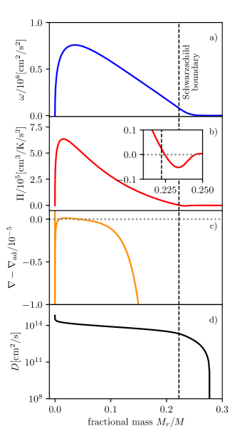
Figure 1: Summary of the interior structure of the convective core of a $5\,M_{\odot}$ main-sequence model, calculated with the 3-equation model. The black dashed line indicates the Schwarzschild boundary. The different panels show a) TKE b) convective flux variable c) super adiabatic temperature gradient and d) the diffusion coefficient according to Eq. (5). The selected stellar model has a central hydrogen abundance of $X_{\rm c}=0.6$. The inset in panel b) shows the region of negative convective flux just beyond the Schwarzschild boundary.

As a representative example, we will first discuss the evolution and the internal structure of a 5 $M_{\odot}$ model applying the 3-equation, non-local convection theory. Figure 1 shows the profiles of the TKE variable $\omega$ (panel a), the convective flux variable $\Pi$ (panel b), the superadiabatic gradient $\nabla-\nabla_{\text{ad}}$ (panel c), where $\nabla$ is the temperature gradient resulting from the convection model, and the diffusion coefficient according to Eq. (5) on a logarithmic scale (panel d). The TKE clearly extends beyond the Schwarzschild boundary, which we compute as usual as the point where $\nabla_{\text{ad}}=\nabla_{\text{rad}}$. Such a behaviour cannot be observed in MLT models, as it is a direct result of the non-local terms in the Kuhfuß convection model. The associated diffusion coefficient shows a rather high value beyond the Schwarzchild boundary and throughout the overshooting zone. This will increase the size of the mixed convective core and therefore naturally create an overshooting zone. Given the profile of the diffusion coefficient, the chemical mixing will resemble the step overshooting rather than the diffusive overshooting scheme. The convective flux variable shows a region of negative flux beyond the Schwarzschild boundary. In the lower panel of Fig. 4 the region of negative convective flux is shown enlarged in the inset (likewise for the convective flux variable $\Pi$ in the middle panel of Fig. 1). This is due to the braking of the convective motions in the stable, radiative stratification. The extent and magnitude of the negative convective flux are very comparable to early results from Xiong (1986), who found that the convective flux penetrates less deeply into the stable layers than for example the kinetic energy and has a nearly negligible magnitude compared to the total flux.

Finally, panel c) shows the superadiabatic temperature gradient of this stellar model (notice the vertical scale). In the inner part of the convection zone the model shows a very small superadiabatic gradient as it is expected for regions with convective driving. At a fractional mass of about 0.05 the temperature gradient drops below the adiabatic value. In contrast to local models this point does not coincide with the formal Schwarzschild boundary, however, the sign change happens substantially before the formal boundary. At the formal Schwarzschild boundary, the temperature gradient has dropped to about $\mathcal{O}(10^{-3})$ below the adiabatic value. The comparison of panels b) and c) shows that there exists an extended region in the model in which the convective flux is positive while the temperature gradient is already subadiabatic. This region is also known as a Deardorff layer (Deardorff 1966) and has been observed in simulations of stellar convection (Chan & Gigas 1992; Muthsam et al. 1995, 1999; Tremblay et al. 2015; Käpylä et al. 2017; Kupka et al. 2018) or other Reynolds stress models (Kupka 1999a; Xiong & Deng 2001; Kupka & Montgomery 2002; Montgomery & Kupka 2004; Zhang & Li 2012).

Such a layer cannot exist in convection models, which do not have enough degrees of freedom. In MLT and the Kuhfuß 1-equation model, the convective flux is directly coupled to the superadiabatic gradient and the convective velocities (see Eq. 4 for the 1-equation model). This of course inhibits any region in which the convective flux and the superadiabatic gradient have a different sign like in the Deardorff layer and forces the convective flux and the TKE to have the same penetration depth. The 3-equation model lifts the strong coupling of convective flux and superadiabatic gradient by directly solving for two more variables ($\Pi$ and $\Phi$) and therefore allows for the existence of such a layer. Deardorff (1966), in the case of atmospheric conditions, argued that it is mainly the non-local term in the equation for $\Phi$ which supports the positive heat flux for subadiabatic temperature gradients (see also Sec. 13 of Canuto 1992, and references therein). The diffusion term $\mathcal{F}_{\Phi}$ in the equation for the entropy fluctuations Eq. (3) acts as a source of entropy fluctuations even though no local source (a superadiabatic temperature gradient) is present. This allows for the outward directed transport of entropy fluctuations, that is a positive convective flux even in subadiabatic layers. This has little impact on the stellar structure and evolution, as the temperature gradient remains nearly adiabatic, and the whole convection zone is chemically well mixed. The existence of such a layer is therefore expected, and confirms the physical relevance of the 3-equation Kuhfuß model. The extent of this layer is difficult to determine from a priori arguments, and asteroseismic analyses might provide observational constraints in the future.

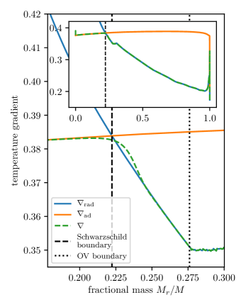
Figure 2: Temperature gradients in the overshooting zone of the same $5\,M_{\odot}$ main-sequence model as in Fig. 1. The blue and orange lines indicate the radiative ($\nabla_{\text{rad}}$) and adiabatic ($\nabla_{\text{ad}}$) temperature gradients, respectively. The green dashed line indicates the model temperature gradient $\nabla$ obtained from the 3-equation non-local convection model. The black dashed line indicates the Schwarzschild boundary, while the black dotted line indicates the boundary of the well mixed overshooting region. The inset shows the three temperature gradients from the centre to the surface of the stellar model. The selected stellar model has a central hydrogen abundance of $X_{\rm c}=0.6$.

In Fig. 2 we show the temperature gradients in the overshooting zone of the same $5\,M_{\odot}$ main-sequence model as in Fig. 1. At the formal Schwarzschild boundary the model temperature gradient has already a slightly subadiabatic value as discussed previously. Beyond the Schwarzschild boundary, the model temperature gradient does not drop to the radiative gradient immediately. Instead, it gradually transitions from slightly subadiabatic to radiative values in a rather narrow mass range. As a consequence, the model temperature gradient takes slightly super-radiative values in this transition region. However, the temperature gradient reaches a radiative value well before the boundary of the mixed region, indicated with the black dotted line in Fig. 2. Considering the small extent of the super-radiative region and the small deviation from the radiative temperature gradient, the overshooting zone in the 3-equation non-local model is mostly radiative. We would like to point out that the shape of the temperature gradient is not subject to assumptions about the thermal stratification (e.g. adiabatic, radiative or any gradual transition between both) in the overshooting zone but instead is a result of the convection model. In the transition region, the convective flux is negative due to the buoyancy braking, which effectively means that energy transport by convection is directed inwards instead of outwards. This effect is counter-balanced by increasing the energy transport by radiation, through an increased model temperature gradient (e.g.  Chan & Sofia 1996).

The temperature gradient of the 3-equation model is comparable to results of different TCM approaches (Xiong & Deng 2001; Li & Yang 2007) for the base of the solar convective envelope. Both Zhang & Li (2012) (their Figs. 6 and 7) and Xiong & Deng (2001) (their Fig. 8) find a temperature gradient that transitions gradually from the adiabatic to the radiative value. They also find a Deardorff layer with a degree of subadiabaticity at the formal Schwarzschild boundary comparable to our findings. From the convective flux as presented in Xiong (1986) one also would expect a similar temperature gradient in the overshooting zone. Furthermore, the shape of the model temperature gradient is also in qualitative agreement with the discussion in Viallet et al. (2015). They argue that under the physical conditions in convective cores, in regions of overshooting efficient chemical mixing and a gradually transitioning temperature gradient are expected. In the 3-equation non-local model, the extent of the nearly adiabatic overshooting zone is controlled by the shape of the negative convective flux in the overshooting zone. For smaller (more negative) values of the convective flux (i.e. more efficient buoyancy braking) the temperature gradient is expected to be closer to the adiabatic value, while for larger (less negative) values it will be closer to the radiative temperature gradient. In Eq. (1) the negative convective flux and the dissipation term act as sink terms in the overshooting zone. Hence, the behaviour of the dissipation term will impact also on the convective flux and in turn on the value of the temperature gradient in the overshooting zone. In computations with the 1-equation non-local version of the theory, the negative convective flux is the dominant sink term for the TKE and the actual dissipation term is negligible (see Fig. 8 of Paper I). This leads to more negative values of the convective flux and thus to a mostly adiabatic temperature gradient in the overshooting zone. We will discuss this in more detail in Sec. 5.1 (see also Fig. 10).

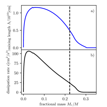
Figure 3: Dissipation length scale $\Lambda$ (a) and dissipation rate (b) in a $5\,M_{\odot}$ main-sequence model. Same stellar model as in Fig. 1. The vertical dashed line indicates the Schwarzschild boundary of the model.

As discussed above and in Paper I we have implemented the increase of the dissipation rate in the overshooting zone through a decrease of the dissipation length scale $\Lambda$. In the original version, Kuhfuß (1987) models the dissipation of the TKE by a Kolmogorov-type term ($\epsilon=C_{D}\omega^{3/2}/\Lambda$ with $\Lambda(r)$ as in Eq. 10). The dissipation length scale $\Lambda$ describes the scale over which the kinetic energy is dissipated such that in the Kolmogorov model, at fixed TKE, a shorter length scale results in an increased dissipation rate. In Fig. 3 we show the length scale $\Lambda$ (panel a) and the dissipation rate (panel b) computed in the same stellar model as in Fig. 1. At a fractional mass of about 0.05 the profile of the dissipation length scale shows a slight kink in this model, where the transition starts. At about 0.28 in fractional mass, the dissipation length scale $\Lambda$ drops to zero, which means that convective motions stop at that point. This coincides with the dying of the TKE beyond the Schwarzschild boundary, as seen in Fig. 1, panel a). The onset of the decrease of the dissipation length scale $\Lambda$ also coincides with the sign change of the superadiabatic gradient (see Fig. 1, panel c). Towards the centre of the model, the dissipation length scale $\Lambda$ drops to zero as well. This is a result of the Wuchterl (1995) correction, also used in our implementation (cf. Paper I). We have also investigated the prescription of Roxburgh & Kupka (2007) as an alternative to that one of Wuchterl (1995) but found little difference with respect to the overshooting region (see also Paper I).

Parameter sensitivity.

We explore some of the parameter dependencies in Appendix B. We studied the impact of the new parameter $c_{4}$, appearing in Eq. (7) (see also Eq. 21 in Paper I), on the structure of the convective core. A comparison of TKE profiles for different values of $c_{4}$ is shown in Fig. 12. The comparison demonstrates that although the parameter has some impact on the overshooting extent, the main properties of the model are not changed substantially. The parameter $\alpha_{\omega}$ , appearing in Eq. (1), controls the non-local flux of the turbulent kinetic energy. Because this flux is mainly responsible for the extension of the kinetic energy beyond the Schwarzschild boundary, one expects that this parameter impacts on the overshooting distance. Figure 13 shows a comparison of different hydrogen profiles of a 5 $M_{\odot}$ star computed with different values of $\alpha_{\omega}$. For a higher value of the parameter, the size of the convective core is larger throughout the evolution of the model. Smaller parameter values reduce the convective core size. Although Kuhfuß (1987) provides a default value for $\alpha_{\omega}$, this value is not known a priori from the theory. Hence, a calibration will be necessary, for example from observations or 3D hydrodynamic simulations. The parameters of the non-local terms in the $\Pi$ and $\Phi$ equations $\alpha_{\Pi}$ and $\alpha_{\Phi}$, appearing in Eq. (2) and (3) respectively, have a negligible impact on the overshooting extent (see Fig. 15 in the appendix). Instead, they have a larger impact on the temperature gradient as the variables $\Pi$ and $\Phi$ are more closely related to the temperature structure. By increasing the parameter $\alpha_{\Pi}$, the magnitude of the superadiabatic gradient increases, while the extent of this region stays the same. Decreasing the value of the parameter $\alpha_{\Phi}$ is increasing the size of the superadiabatic region, therefore reducing the size of the Deardorff layer, while the magnitude stays the same. This is expected because the non-local term in the $\Phi$ equation is the one which is driving convection in the Deardorff-layer.

3.2 Comparison to MLT

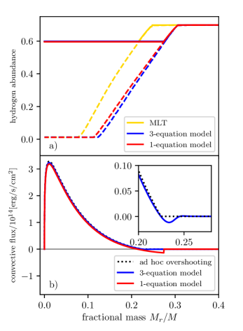
Figure 4: Comparison of models (yellow lines) using MLT without overshooting to those computed with the 3-equation theory (blue lines) and the 1-equation model (red lines). Panel a) compares the hydrogen profiles at an early stage on the main sequence, when $X_{\rm c}=0.6$ (solid lines), and at the end of it ($X_{\rm c}\approx 0$; dashed lines). Panel b) shows the convective fluxes of an MLT model with diffusive overshooting (dotted black line), a 3-equation model (solid blue line) and a 1-equation model (solid red line). These models have been selected to have the same central hydrogen abundance of $X_{\rm c}=0.6$ and the same chemically homogeneous core size.

Mixing-length theory is still the most commonly used theory to describe convection in stars. Therefore, we will now compare the results of the 3-equation model with results obtained from standard MLT, that is without and with an additional treatment of overshooting. The fractional hydrogen abundances early on and at the end of the main sequence computed with the 3-equation model and an MLT model without overshooting are shown in the upper panel of Fig. 4. At the same central hydrogen abundance, the fully mixed region of the 3-equation model always extends past that of the MLT model. This is comparable to models which include ad hoc overshooting beyond the formal Schwarzschild boundary. In contrast to the ad hoc overshooting models, the overshooting in the 3-equation model results from the solution of the model equations. The lower panel of Fig. 4 shows a comparison of the convective fluxes in the 3-equation model and an MLT model. Both models have been selected to have the same central hydrogen abundance. Ad hoc overshooting has been included in this MLT model, and tuned in such a way as to obtain a model with the same core size as obtained from the 3-equation model. In the bulk of the convection zone, both fluxes show very close agreement. Beyond the Schwarzschild boundary, the narrow region with negative convective flux in the non-local model can be identified. This region is shown enlarged in the inset.

Finally, in Fig. 5 we compare the evolutionary tracks of the 3-equation model, indicated by the solid blue line, with an MLT model without ad hoc overshooting (yellow line) and an MLT model including ad hoc overshooting (black line). The black dot indicates the position of the stellar model with $X_{\rm c}=0.6$ discussed in subsection 3.1 in Figs. 1 to 4. The computation of the 3-equation model starts at the beginning of the main sequence from an MLT model including diffusive overshooting as described above and then evolves through core hydrogen burning up until core hydrogen exhaustion. Compared to the MLT model, the non-local model shows a higher luminosity throughout the main sequence, as expected for the larger convectively mixed core.

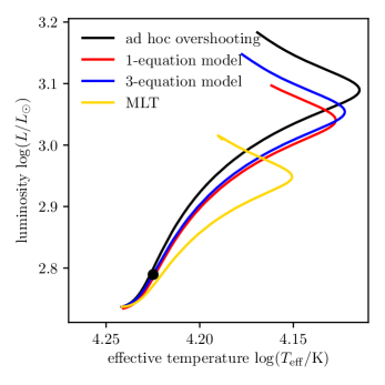
Figure 5: Evolutionary tracks in the Hertzsprung-Russell diagram of a $5\,M_{\odot}$ model computed with MLT, shown with a yellow line, ad hoc overshooting, shown with a black line, and the 3-equation, non-local model, shown with a solid blue line. The black dot marks the model selected at a central hydrogen abundance of $X_{\rm c}=0.6$.

3.3 Comparison to the 1-equation non-local models

In addition to the 3-equation non-local models, we have also computed stellar models, in which convection is described by the 1-equation model (see Sec. 2.1). As before, we included the non-local terms. Figure 6 shows a comparison of the TKE profiles for the 1- and 3-equation, non-local models on a logarithmic scale. The TKE on a linear scale can be found in Fig. 11 in the appendix. The models have been selected at the same central hydrogen abundance to ensure that they are in the same evolutionary stage. This shows that the overshooting extent in the 1-equation non-local model is very comparable to the 3-equation non-local model for the same choice of the parameter $\alpha_{\omega}$. The overall behaviour of the 1-equation non-local model and the new 3-equation non-local model looks very similar. The overshooting extent is clearly limited, and there is a steep drop in the TKE at the overshooting boundary. Also, the absolute values of the TKE look comparable in the bulk of the convection zone (Fig. 11). We will analyse the absolute value of the TKE in more detail below. We note that this result is obtained without tuning the parameters of the models. For the parameters which both models have in common, the same values were chosen. In the overshooting zone, the 3-equation model has much smaller TKE than the 1-equation model. Nevertheless, the energies are still high enough to fully mix the overshooting region in the 3-equation model.

In the upper panel of Fig. 4 we compare the hydrogen profiles of the 1-equation model with the results from the 3-equation model and an MLT model at the beginning and at the end of the main-sequence. As expected from the similar TKE profiles shown in Fig. 6 the hydrogen profile of the 1-equation model extends past the local MLT model and looks very similar to the 3-equation model. Towards the end of the main-sequence, the 1-equation model has a smaller core than the 3-equation model, leading to a slightly different slope in the hydrogen profiles. Likewise, the evolutionary track shown in Fig. 5 of the 1-equation model looks very similar to the 3-equation model. Towards the end of the main-sequence, the luminosity is slightly lower owing to the smaller convective core. In the lower panel of Fig. 4 we compare the convective flux of the 1-equation model to the 3-equation model and an MLT model including ad hoc overshooting. As for the 3-equation model, the convective flux shows close agreement with the other two models in the bulk of the convection zone. Only in the overshooting zone, where the convective flux becomes negative, discrepancies become apparent. Compared to the 3-equation model, the zone of negative convective flux is more extended and the absolute value is larger, that is the convective flux is more negative. This can be attributed to the parametrisation of the convective flux in the 1-equation model according to Eq. (4). As discussed in Sec. 4 of Paper I (see also their Fig. 8) the buoyancy term, proportional to the convective flux, acts as the main sink term in the overshooting zone, requiring larger absolute values in the overshooting zone. We would like to note that this strongly negative convective flux in the overshooting zone will also cause the 1-equation model to have a nearly adiabatic overshooting zone, as compared to the nearly radiative overshooting zone in the 3-equation model.

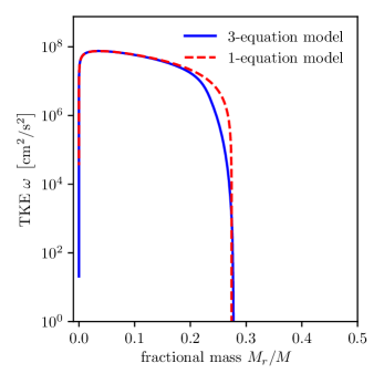
Figure 6: Comparison of the TKE in the 1-equation non-local model and the 3-equation non-local model with enhanced dissipation rate of TKE in a 5 $M_{\odot}$ main-sequence model on a logarithmic scale. The models have been selected to have the same central hydrogen abundance as the model in Fig. 1. The 1-equation model computes $\Lambda$ according to Eq. (10).

4 Non-local convection for varying initial masses

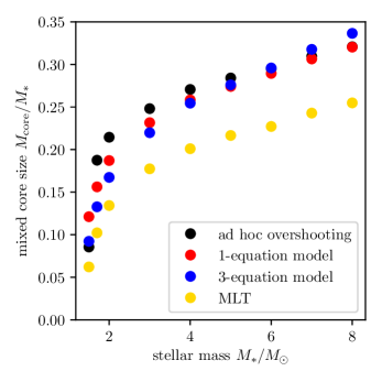
Figure 7: Comparison of mixed core sizes of stellar models in units of the stellar mass $M_{*}$ over a range of initial stellar masses computed with different convection models. The models with ad hoc overshoot include a geometric cut-off to limit the size of small convective cores in lower mass stars. The models have been selected at a central hydrogen abundance of $X_{\rm c}=0.6$. The MLT models are computed without overshooting.

We computed stellar models in a mass range of 1.5-8 $M_{\odot}$, using the 3-equation non-local model. The models have been constructed in the same way and using the same parameters as for the 5 $M_{\odot}$ model presented so far. For comparison, we have computed three other sets of stellar models with different convection descriptions: (i) with the Kuhfuß 1-equation model to compare the results of the 3-equation model to a simpler TCM; (ii) with MLT plus diffusive overshooting as described by Freytag et al. (1996) to compare to one of the standard ad hoc descriptions of convective overshooting with the same parameter value $f_{\text{OV}}=0.02$ as discussed above. Finally, (iii), we computed MLT models without overshooting to compare the results to a local convection theory. At least in terms of core size and temperature structure, models using the local Kuhfuß theories would be equivalent to MLT models. For the Kuhfuß theory, we used the same value of 0.3 for the parameter $\alpha_{\omega}$, as before. To allow for a comparison across the mass range and the different convection descriptions, the models are selected at the same central hydrogen abundance of $X_{\rm c}=0.6$.

Figure 7 shows the sizes of mixed cores in models derived from these four descriptions of convection and convective overshooting over a range of initial masses. For all masses under consideration, the mixed core from the 3-equation model is larger than the convective core from an MLT model, as expected. This shows that when applying the 3-equation model, an overshooting zone emerges across the whole mass range investigated. Comparing the 3-equation model to the 1-equation model and the ad hoc overshoot model, the mixed core sizes show good qualitative agreement. We repeat that this is achieved without fine-tuning any of the involved parameters. The relative size of the mixed cores decreases with decreasing stellar mass for all four descriptions, but differences in the details between the different convection descriptions are evident. For higher masses, the derived values for the mixed core sizes are almost identical among the ad hoc overshooting and the 1- and 3-equation Kuhfuß models. For low stellar masses, the results show larger discrepancies. Stellar models applying the 3-equation non-local model have the smallest cores, and the core size decreases faster with decreasing stellar mass than in the 1-equation models and the ad hoc overshoot models. As the ad hoc overshoot model has been calibrated to observations, this allows at least for an indirect comparison of the 1- and 3-equation model with observations.

In addition to the core sizes, we have also analysed the absolute values of the convective velocities. The Kuhfuß model does not solve for the convective velocity itself, but rather for the TKE $\omega$. We approximate the mean convective velocity from the TKE by assuming full isotropy:

$$v_{\text{c,iso}}=\sqrt{\frac{2}{3}\omega}\,.$$ (11)

When using MLT, the convective velocities are computed as:

$$v_{c}=\frac{1}{\sqrt{8}}\left(\frac{g}{H_{p}}\right)^{1/2}\Lambda\left(\nabla-\nabla_{\mathrm{ad}}\right)^{1/2}\,,$$

(e.g. Kippenhahn et al. 2012). The computation of convective velocities is the same in MLT models with and without diffusive overshoot, as the inclusion of ad hoc overshooting does not impact on the description of convection. To compare MLT and the Kuhfuß-theories we evaluate the maximum convective velocity in the convection zone. The maximum is reached well within the Schwarzschild boundaries for all models, and therefore allows for a consistent comparison.

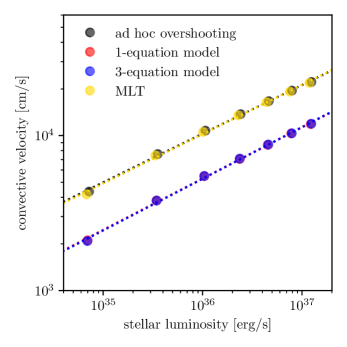
Figure 8: Comparison of the maximum convective velocities for different convection models as a function of stellar luminosity. For the Kuhfuß model, the isotropic convective velocity $v_{\text{c,iso}}$ is plotted. The dotted lines indicate a linear fit to the logarithmic data. Please note that the data of the 1- and 3-equation Kuhfuß-models (red and blue points respectively) are largely overlapping, as well as the black and yellow dots.

We show this comparison of the maximum convective velocities in the core as a function of stellar luminosity in Fig. 8. The convection descriptions are the same as in Fig. 7. For all cases, the scaling relation of the convective velocities has the same slope. A linear fit (dotted lines) to the data results in a value of $\sim 0.3$ for all of them. However, the absolute values from the Kuhfuß and MLT models differ by a constant factor of about two, indicated by the offset between the two pairs of lines. This difference in the absolute value is the result of two different effects. The change of the mixing length has the largest impact on the velocity. A reduced mixing length will lead to an increased dissipation rate and smaller velocities as a consequence. In the Kuhfuß models we use a smaller value of $\alpha=1$ as obtained by a solar calibration instead of $\alpha=1.6$ for the MLT models. In addition, the mixing length is reduced towards the centre according to the Wuchterl (1995) formulation (see Eq. 6). The convective velocity is reduced further compared to the local MLT models by taking the non-local terms into account, which act as a sink term in the bulk of the convection zone. The slope of 0.3 is very close to the $v_{\text{c}}\propto L^{1/3}$ scaling relation expected from MLT. This comparison also demonstrates that the absolute values of the TKE are very similar between the 1- and the 3-equation Kuhfuß theories over the full mass range. For the $5\,M_{\odot}$ model, this was already apparent when comparing the TKE profiles in Fig. 6.

5 Discussion

5.1 Relation between 1- and 3-equation model

As discussed in Sec. 2.1 the 1-equation model is a simplification of the 3-equation model, for which Kuhfuß (1987) assumes that the convective flux is proportional to the super-adiabatic temperature gradient and the square-root of the TKE. This allows removing two of the three equations, namely for the entropy fluctuations $\Phi$ and the velocity entropy correlations $\Pi$. The equation for the TKE $\omega$ remains unchanged. The approximation for the convective flux allows expressing the temperature gradient as a function of the TKE. This couples the thermal structure and the TKE very closely. In the 3-equation model, the convective flux is evolved with an additional equation, which reduces the coupling of the thermal structure and the TKE. Despite the increased model complexity, the behaviour of the TKE in the 1- and 3-equation model is quite similar, as seen in Fig. 6.

In the bulk of the convection zone, both models result in the same absolute value of the TKE. This can be also seen in Fig. 8 by the agreement between red and blue points for a wider mass range. It can be attributed to the similarity of the equations. The additional dissipation is not or only weakly operating in the bulk of the convection zone. Hence, both the dissipation and the non-local term have the same functional form. The convective flux is adjusted such that a nearly adiabatic stratification is achieved in both models; therefore, the buoyancy term is also very comparable in the 1- and 3-equation models. As soon as the temperature gradient becomes subadiabatic, which happens already well within the Schwarzschild boundary in the 3-equation model, the dissipation by buoyancy waves is taken into account. This means that the functional form of the dissipation term changes. Due to the difference in the thermal structure in this region also the convective flux looks different. This will lead to a different solution for the TKE in the overshooting zone, as is evident from Fig. 6 towards the edge of the convection zone.

The main difference between the 1- and 3-equation model is probably the temperature stratification which results from the solution of the model equations. Due to the coupling of the convective flux to superadiabatic gradient and convective velocities in the 1-equation model, the convective flux is forced to have the same penetration depth into the stable layers as the TKE and at the same time to have the same sign as the superadiabatic gradient. As seen in our models and pointed out by Xiong & Deng (2001) this strong coupling leads to a nearly adiabatic temperature gradient in the overshooting zone and prevents the existence of a Deardorff layer (see also Paper I). Also with respect to other models of convection (e.g. MLT) the existence of a large subadiabatic zone in the convective region for the case of the 3-equation model is striking. To better understand the behaviour of the temperature gradient in the overshooting zone, we will analyse it in terms of the Peclet number. The Peclet number is the ratio of the timescales of radiative and advective transport and can be interpreted as an indicator for convective efficiency. A common definition of the Peclet number is:

$$\text{Pe}=\frac{u\cdot l}{\chi}$$

where $u$ and $l$ are a typical velocity and length-scale of the convective flow. The radiative diffusivity is defined as

$$\chi=\frac{16\sigma T^{3}}{3\kappa\rho^{2}c_{p}}\,.$$

As a typical convective velocity we use again the isotropic velocity, Eq. (11). Due to the usage of typical scales for velocities and length-scales which are not rigorously defined, the interpretation of absolute values of the Peclet number remains difficult. Hence, we will only look at ratios of the Peclet number to compare different models. We will also assume that the length-scale and the radiative diffusivity are the same, when comparing different models. Under these assumptions, it is easy to see that:

$$\frac{\text{Pe}_{1}}{\text{Pe}_{3}}\propto\sqrt{\frac{\omega_{1}}{\omega_{3}}}$$

The ratio of the Peclet numbers obtained for the 1- and 3-equation models for a $5\,M_{\odot}$ main-sequence model is shown in Fig 9. In the bulk of the convection zone, the 1- and 3-equation models have very similar Peclet numbers, which means the transport of energy by convection behaves very comparably. In the overshooting zone, however, the 1-equation model has a Peclet number which is up to 7 times higher than that of the 3-equation model. This indicates that convection as described by the 1-equation model is much more efficient in the overshooting zone than when described by the 3-equation model.

This change in efficiency will also impact the temperature gradient. Following the approximation of the convective flux in the 1-equation model, the convective flux scales as $\Pi\propto\sqrt{\omega}$. Using the ratio of the Peclet numbers, one can therefore write a Peclet-scaled convective flux

$$\Pi_{3,\text{Pe}}=\Pi_{1}\cdot\frac{\text{Pe}_{3}}{\text{Pe}_{1}},$$ (12)

to mimic the convective flux in the 3-equation model. The resulting convective flux is shown with a blue dashed line in the upper panel of Fig. 10. Using this scaled convective flux, a scaled temperature gradient can be computed, as illustrated by the green dashed line in the lower panel of Fig. 10. For comparison, the model temperature gradients of the 1- and 3-equation model are visualized by a green dotted and solid line, respectively.

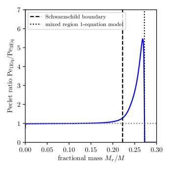
Figure 9: Ratio of the Peclet numbers for the 1- and 3-equation models for a $5\,M_{\odot}$ main-sequence model.

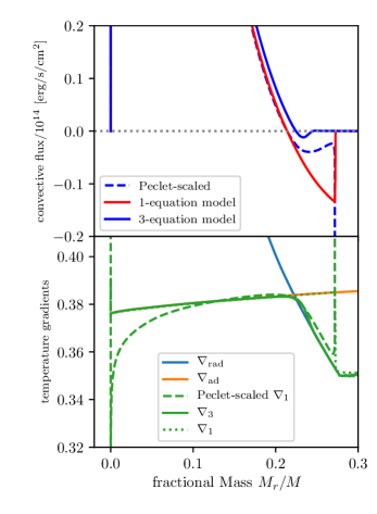
Figure 10: Upper panel: Convective flux as a function of fractional mass. The red and the blue lines show the results obtained from the 1- and 3-equation model, respectively. The blue dashed line indicates the convective flux scaled with the Peclet number according to Eq. (12). Lower panel: Temperature gradients as a function of fractional mass. The blue and orange lines indicate the radiative and adiabatic temperature gradient, respectively. The green dotted and solid lines indicate the temperature gradient as obtained by the 1- and 3-equation models. The green dashed line shows the temperature gradient of the 1-equation model computed from the scaled convective flux shown in the upper panel.

This comparison confirms that the reduced convective efficiency obtained from the Peclet numbers is sufficient to change the behaviour of the temperature gradient from nearly adiabatic to more radiative in the overshooting zone, and implies that the behaviour of the temperature gradient in the overshooting zone can at least qualitatively be predicted from the TKE alone without invoking the other convective equations for $\Pi$ and $\Phi$. The fact that the region of negative values in the scaled convective flux is more extended compared to the actual convective flux from the 3-equation model is due to the different penetration depths of TKE and convective flux in the 3-equation model. We conclude that this is an important indication for internal consistency of the model. It furthermore shows that the mostly radiative temperature gradient in the overshooting zone is in fact a result of reduced convective efficiency in the overshooting zone in the 3-equation model. Following the terminology proposed by Zahn (1991), in the 1-equation model the overshooting zone is best described by subadiabatic penetration while the more inefficient convection in the 3-equation model concerns overshooting of chemical element distributions only.

Considering the chemical mixing, both models will result in a more step-like chemical mixing profile. The extent of the mixed region is mainly dependent on the choice of the parameter $\alpha_{\omega}$, as discussed in Appendix B. This parameter cannot be determined from first principles. As for the ad hoc descriptions of convective core overshooting, a calibration of this parameter is required, which will be discussed below. Furthermore, the resulting convective flux is also very similar in the bulk of the convection zone and differences become only obvious in the overshooting zone. Given the relative freedom in choosing $\alpha_{\omega}$ and the similarity in the mixing properties of both models, resulting stellar models are basically indistinguishable when comparing the chemical structure. Once the observations become sensitive enough to the thermal structure in the overshooting zone as, for example, with the help of asteroseismology (Michielsen et al. 2019), it will become possible to detect differences between both models. In view of the general agreement between 1- and 3-equation model, the application of the 1-equation model seems to be sufficient to obtain the chemical structure from a non-local convection model. The parameter $\alpha_{\omega}$ can be tuned to obtain the correct size of the convective core. However, the stratification obtained from the 1-equation model is less realistic.

5.2 Other constraints on core overshooting

To date, a range of different approaches to determine the extent of convective cores has been followed. In this subsection, we discuss a few examples of convective core size determinations. The need for a larger mixed core has been recognized already in the ’80s of the last century (see, for example, Bressan et al. 1981 in relation to the Hertzsprung-Russell-diagram of massive stars, or Maeder & Mermilliod 1981 concerning that of open clusters). In the latter case, isochrones derived from stellar models which include core overshooting match the morphology of the turn-off region better than models without overshooting (Pietrinferni et al. 2004; Magic et al. 2010). The comparison to observations showed further that the overshooting distance in terms of pressure scale heights needs to increase with mass in the range between 1.2 and $\sim 2\,M_{\odot}$. This mass dependence can be included explicitly in the computations by expressing the overshooting parameter as a function of the total stellar mass. Alternatively, this mass dependence can also be introduced in the stellar models by limiting the radial extent of the overshooting zone geometrically. In both cases, the parameter of the overshooting scheme effectively needs to increase with stellar mass. For the TCM, however, this is a natural outcome without imposing it.

Eclipsing binary systems offer an excellent opportunity to put constraints on stellar physics. Claret & Torres (2019) used a large sample of eclipsing binaries to determine the overshooting parameter as a function of mass. They find a clear increase of the overshooting parameter (extent) with mass, even though the statistical significance of this result has been debated (Constantino & Baraffe 2018). In a detailed analysis, Higl et al. (2018) addressed the evolution of the binary system TZ Fornacis with an evolved red giant primary and a main-sequence secondary star, both with masses of $\sim 2\,M_{\odot}$. They found that a basically unrestricted overshooting extent, using the standard value for the free parameter, is required to explain the evolution of this system. This puts further constraints on the mass dependence of the overshooting parameter.

The high precision photometric data obtained from space telescopes like Kepler or CoRoT allowed setting further constraints on the stellar evolution models. Using asteroseismology of g-mode pulsators, the convective core masses of intermediate mass stars has been determined for larger samples of stars (e.g. Pedersen et al. 2021; Mombarg et al. 2019). Similarly, the seismology of p-mode pulsators allows determining the required overshooting efficiency in lower mass stars (e.g. Deheuvels et al. 2016; Angelou et al. 2020). In agreement with the previously mentioned studies, they find that the relative mass of the mixed core needs to increase with stellar mass. A more detailed comparison of the TCM models discussed in this work with asteroseismic observations needs to be addressed in future work. Finally, asteroseismology allows probing the temperature gradient in the overshooting zone. Michielsen et al. (2021) inferred a predominantly radiative overshooting zone in a $\sim 3.5\,M_{\odot}$ main-sequence star, which is in agreement with the temperature gradient obtained from the 3-equation model but disagrees with the 1-equation model. However, they point out that this result is only obtained for this single B-type star and might not be generalisable for all B-type stars.

With the increase of computational resources in recent years, more and more multidimensional hydro-simulations of stellar core convection have been carried out (e.g.​ Meakin & Arnett 2007; Gilet et al. 2013; Edelmann et al. 2019; Higl et al. 2021). These simulations confirmed, for example, the scaling of the stellar luminosity with the third power of the convective velocities (e.g. Edelmann et al. 2019; Higl et al. 2021, and references therein). In Higl et al. (2021) the authors calibrate the overshooting parameter $f_{\text{OV}}$ in GARSTEC to 2D simulations of core convection in low and intermediate mass stars. By matching the size of the mixed convective core in the 1D GARSTEC models to the size of the mixed region in the 2D simulations, they find that the effective parameter of $f_{\text{OV}}$ needs to decrease with stellar mass. To limit the size of the convective cores for small stellar mass in the 1D models, they use the geometric “square” cut-off according to Eq. (14). As they use the same stellar evolution code as we do, this allows for a direct comparison of the results. Higl et al. (2021) find that the size of the convective cores resulting from the 2D simulations need to be larger than the GARSTEC models computed including the square cut-off (Eq. 14) at a constant overshooting parameter. This indicates that the geometric square cut-off is too restrictive. As the 3-equation model predicts mixed core masses similar to the GARSTEC models including this geometric cut-off (see Fig. 16) this indicates that our 3-equation model might be too restrictive as well at this lower mass range.

Finally, other TCMs have been used to compute stellar evolution models including the effects of non-local convection. Xiong (1986) has computed stellar models in the mass range of 7 to $60\,M_{\odot}$. He finds that by solving the convection equations, the TKE extends beyond the formal Schwarzschild boundary and that this also increases the size of the mixed region. The size of the well mixed region increases with increasing stellar mass. Both results are in agreement with our findings employing the 3-equation model. Xiong (1986) also finds that the convective flux penetrates much less deeply into the stable layers than the TKE. The magnitude of the convective flux in this region is negligible, which causes the temperature gradient to be mostly radiative in the overshooting region. This is in good agreement with the decoupling of the thermal and the chemical structure we discussed in detail in Sect. 3 and Paper I. Zhang (2016) applied the TCM by Li & Yang (2007) in a similar mass range as in this work. They develop a simplified model comparable to the 1-equation model and find very good agreement between the full model and the simplified version. Li (2017) applies the simplified TCM by Li (2012) to compute stellar models of a $5\,M_{\odot}$ star and find an overshooting distance of about $0.2H_{p}$, which is comparable to the overshooting distance obtained with our 3-equation model.

6 Conclusions

In this work, we have presented results of stellar structure and evolution calculations using the TCM proposed by Kuhfuß (1987). We have implemented the Kuhfuß model into GARSTEC which solves the four stellar structure equations and the three equations of the convection model simultaneously with the implicit Henyey method. We have computed main-sequence models of intermediate-mass main-sequence stars between $1.5$ and $8\,M_{\odot}$ which consistently compute the structure and evolution of the TKE, convective flux, and entropy fluctuations. This naturally includes the effects of convective overshooting for the thermal and chemical structure. In Paper I, we have demonstrated that the original 3-equation model with standard MLT prescription for the dissipation length of TKE leads to convection zones which essentially extend throughout the entire stellar interior. We have therefore implemented the dissipation by gravity waves as discussed in Paper I in addition to the original Kuhfuß model. We showed that the Kuhfuß 3-equation model with an increased dissipation rate results in models with physically reasonable overshooting distances. This indicates that the dissipation was actually underestimated by the original description, and that dissipation by gravity waves is a relevant effect in core overshooting zones.

In Fig. 1 here we have shown a summary of the TKE and flux and the temperature gradient for a convective core of a $5\,M_{\odot}$ main-sequence model. We find that the TKE extends beyond the formal Schwarzschild boundary of convective neutrality. This is the result of the non-local terms in the Kuhfuß model. The convective flux shows a region of negative values beyond the Schwarzschild boundary, which is, however, penetrating less deeply into the stable layers than the TKE. As the convective motions are very efficient in mixing chemical elements, the extended convective core will have essentially the same composition as the convective core. This can be seen in Fig. 4, upper panel, in which the hydrogen profiles at the end of the main-sequence of an MLT and a Kuhfuß 3-equation model are compared. In the Kuhfuß model, this extension beyond the Schwarzschild boundary is the outcome of the solution of the model equations and not due to the inclusion of any sort of ad hoc overshooting. We also compared the results of the full 3-equation model to the simplified 1-equation model and find qualitative and quantitative agreement of the TKE throughout a large part of the convection zone. This is a result of the similarity of the model equations and the chosen parameters, which are the same for both models. In addition to the convective velocity and the associated mixing also the temperature gradient is part of the model solution. This is another important difference compared to ad hoc descriptions of convective overshooting, in which the temperature gradient needs to be assumed separately and independently.

The analysis of the temperature gradient has shown the existence of a Deardorff-layer (Deardorff 1966), in which the temperature gradient is subadiabatic and the convective flux is still positive. The existence of the Deardorff-layer has been confirmed in different numerical simulations of stellar convection (Chan & Gigas 1992; Muthsam et al. 1995, 1999; Tremblay et al. 2015; Käpylä et al. 2017) and other Reynolds stress models (Kupka 1999a; Xiong & Deng 2001; Kupka & Montgomery 2002; Montgomery & Kupka 2004; Zhang & Li 2012). Beyond the Deardorff-layer, the convective flux becomes negative as the result of the stable stratification (cf. also Muthsam et al. 1995 and references in Canuto 1992). In the overshooting region, the model temperature gradient gradually transitions from a slightly subadiabatic to a radiative value, exhibiting a small region with a super-radiative temperature gradient (see Fig. 2). However, this transition region is rather narrow, such that the overshooting zone has a mostly radiative temperature gradient. This is in agreement with very recent results from asteroseismology (Michielsen et al. 2021). In contrast to the 3-equation model, the overshooting zone of the 1-equation model shows a mostly adiabatic temperature gradient. As pointed out by Xiong & Deng (2001) this can be attributed to the assumption of a full correlation between the convective flux and the convective velocities, as it is done in the 1-equation model (see Eq. 4). The approximation Eq. (4) does not allow for a Deardorff layer, as the convective flux is proportional to the superadiabatic gradient. From a theoretical point of view, the existence of a Deardorff-layer can be attributed to the non-local term of the $\Phi$-equation Eq. (3) (Deardorff 1966). This shows that an independent equation for the convective flux is required (see also Kupka 2020) and highlights the necessity to consider more complex turbulence models like the 3-equation model to capture the temperature structure in the overshooting zone more accurately. The comparison of the Peclet numbers of the 1- and 3-equation models shows further that the mostly radiative temperature gradient in the overshooting zone of the 3-equation model can be explained by the reduced TKE/velocities compared to the 1-equation model. The narrow range of the transition region from an adiabatic to a radiative temperature gradient can be attributed to the shallower penetration of the convective flux into the stable layers compared to the 1-equation model.

A comparison with stellar models using MLT shows qualitative agreement of the TKE and the convective flux in the part of the convection zone unstable according to the Schwarzschild criterion ($\nabla_{\rm ad}=\nabla_{\rm rad}$). For the convective flux, we even find a very good quantitative agreement between the Kuhfuß model and MLT in that region (see Fig. 4, lower panel). The convective velocities found in the Kuhfuß model are smaller than in MLT by a factor of two. This qualitative agreement indicates that the stellar structure has the largest impact on the convective properties in the bulk of the convection zone, irrespectively of the convection model in use. The nuclear energy released in the centre determines the convective flux — about 80% of the local flux in the centre — and the coefficients of the convection model determine the absolute values of the other convective variables. Differences appear in the overshooting zone, which is sensitive to more subtle changes in the convection model. In the overshooting zone the stellar flux is mainly transported by radiation, such that the convective structure of this region is less constrained by the stellar structure but a result of the convection model.

The results of the 1- and 3-equation models over a broader mass range show qualitative agreement with other overshoot descriptions. For given values of $\alpha_{\omega}$ and $f_{\rm OV}$, this is achieved without fine-tuning any of the other model parameters, as we have used the closure parameters suggested by the authors of the turbulence model (see Canuto & Dubovikov 1998, and references therein). Tests of those parameters — for different physical scenarios — are published in the literature (Kuhfuß 1986, 1987; Wuchterl 1995; Canuto 1992; Canuto & Dubovikov 1998; Kupka & Muthsam 2007c). In Fig. 7 we have shown a comparison of mixed hydrogen core sizes computed with diffusive overshooting, the 1-equation and the 3-equation model, and MLT. The comparison shows that the exact extent of the convective core depends on the details of the model. For the same parameter choice of the parameter $\alpha_{\omega}$ at lower masses, the 3-equation model shows a reduced amount of overshooting compared to the 1-equation model, while the 3-equation models have larger cores at higher masses. The newly introduced parameters which control the reduction of the dissipation length scale $\Lambda$ were shown to have a moderate impact on the overshooting extent. For its default overshoot parameter, the diffusive mixing model produces yet larger mixed core sizes. Towards the lower end of the mass range, both Kuhfuß models show a decrease of the mixed core size as implemented by other methods to match observations from open clusters and binaries (Claret & Torres 2019; Pietrinferni et al. 2004; Magic et al. 2010). Higl et al. (2018) found that the overshooting parameter needs to increase steeper with mass than predicted by GARSTEC including the geometric square cut-off from the analysis of the TZ For binary system. In agreement with the conclusion from the 2D simulations, (Higl et al. 2021) this indicates that the convective core size predicted by the 1- and 3-equation model increases too shallowly with stellar mass for a constant parameter $\alpha_{\omega}$. To match the observations and the results from the 2D simulations, this would require to modify the parameter $\alpha_{\omega}$ as a function of mass. Further constraints on the parameter $\alpha_{\omega}$ can be obtained by comparing the Kuhfuß model to results from asteroseismology of intermediate mass stars.

However, such tuning of $\alpha_{\omega}$ seems non-advisable: the physical incompleteness of the ad hoc model of convective overshooting, as an example, is well demonstrated by the shrinking of the convective core size with mass for stars with $M<2\,M_{\odot}$ not only requiring an extra cut-off function (Eq. 14) to limit the convective core size to values compatible with observations, but even demanding a more fine-tuned function (Eq. 15) to pass such a stringent test. While applying a similar procedure to $\alpha_{\omega}$ as for $f_{\text{OV}}$ appears to be a convenient ad hoc solution to match exactly the observational data, it provides no new insights and requires redoing similar procedures in related, but different scenarios. Finding the physical reason for the remaining, now already much smaller discrepancies with the data, on the other hand, might allow for a model not requiring such measures in other applications either (cf. also the discussion on such requirements in Kupka & Muthsam 2017).

Our study of stellar models applying the 3-equation model from Kuhfuß (1987) has shown that the resulting stellar structure depends sensitively on the details of the convection model. Although the original 1- and 3-equation theories are very closely related, their application results in very different structures of the convection zone (see Paper I). We demonstrated that modifying the dissipation term of the TKE can remedy this discrepancy. The improved 3-equation model compares very well with the 1-equation model, both in terms of the TKE and the mixing properties. For applications in which the temperature structure of the overshooting zone is not important, the 1-equation model describes the convective core similarly well as the 3-equation model. The parameter $\alpha_{\omega}$ allows obtaining the required convective core size to match with the observations. Only when the thermal structure of the overshooting zone is of major interest, a more complex convection model like the 3-equation model needs to be used. A self-consistent prediction of the detailed convective core structure appears to require a physically more complete (and thus more complex model). As discussed above, at least three equations are required to allow for more complex phenomena like, for example, a Deardorff layer. In Canuto & Dubovikov (1998) further partial differential equations for the dissipation rate and the vertical component of the TKE are discussed. This potentially allows removing some of the simplifications still present in the 3-equation model. However, increasing the number of equations comes at the price of gaining numerical complexity. Including these equations into stellar structure and evolution models has to remain the task of future work. Finally, a comparison with more and more realistic 3D hydro-simulations of convective cores will be useful to put further constraints on our TCM model, in particular to restrict closure conditions. This is presently under way (Ahlborn & Higl, in preparation). The application of the extended 3-equation Kuhfuß model to stellar envelopes will be presented in another forthcoming paper (Ahlborn et al. 2022, in preparation). In any case, turbulent convection models offer a convincing and feasible improvement of the treatment of convection in 1D stellar models beyond the standard mixing-length theory.

Appendix A Comparison of 1- and 3-equation model

Figure 11 shows the TKE in the 1- and 3-equation model on a linear scale. Even though the TKE of the 3-equation model has approximately the same extent as the 1-equation model as seen in Fig. 6 it drops off faster. Despite the smaller values of the TKE the efficiency of the chemical mixing is still high enough to fully mix the overshooting region. Therefore, the chemical profiles obtained from the 1- and 3-equation model are very comparable.

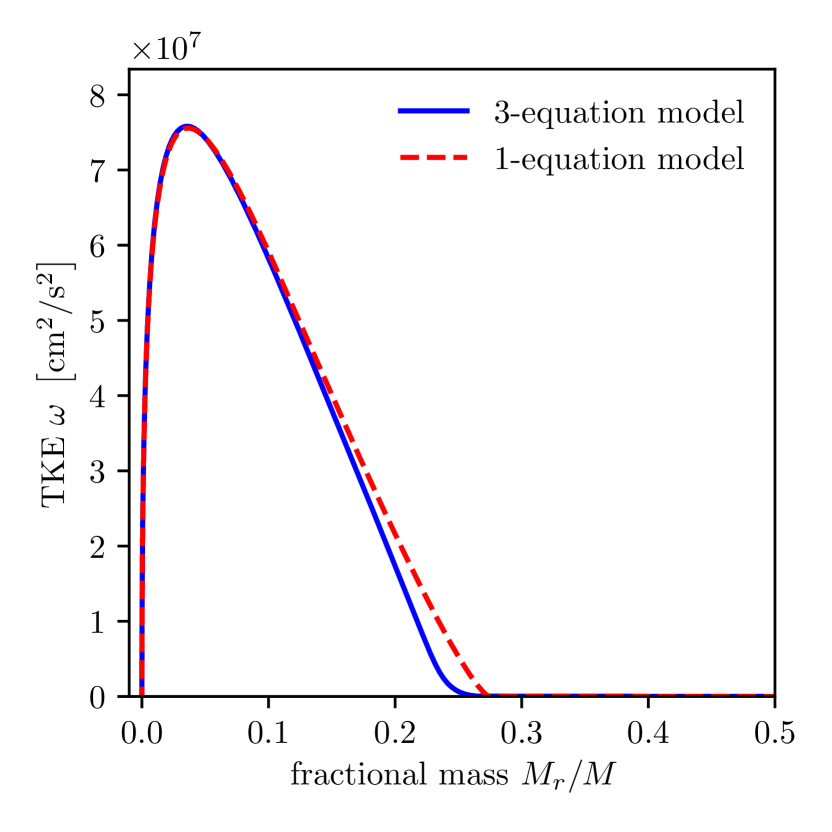
Figure 11: Comparison of the TKE of the 1-equation and 3-equation non-local models in a $5\,M_{\odot}$ main-sequence model with limited dissipation length scale $\Lambda$ for the 3-equation model.

Appendix B Parameter dependence

The model for the modification of the dissipation length scale comes with a number of parameters ($c_{2},c_{3},c_{\epsilon}$). These parameters are not necessarily free, but have been calibrated in the framework of the convection models developed by Canuto (1992). These parameters enter the equation of the reduction factor as a single parameter, which was previously defined as $c_{4}$. Given the dissipation parameter of the 3-equation model, we find $c_{4}\approx 0.072$ while for the dissipation parameter of the Canuto & Dubovikov (1998) model $c_{4}\approx 0.2$ as described in Paper I. As mentioned already in Sect. 3.6 in Paper I, the effect of changing $c_{\epsilon}$ on changing $c_{4}$ to some extent cancels out in the calculation of $\Lambda$, as $c_{\epsilon}$ appears in the denominator of $c_{4}=c_{3}/(c_{2}c_{\epsilon})$ and in the numerator of $\Lambda=c_{\epsilon}\omega^{3/2}/\epsilon$. Hence, if $c_{4}$ is adjusted according to $c_{4}=c_{3}/(c_{2}c_{\epsilon})$, a change of $c_{\epsilon}$ first of all influences the TKE dissipation rate $\epsilon$ throughout the whole model and is not specifically changing $\epsilon$ only within the overshooting zone. To check which impact these parameters actually have on the result, we varied their values. As they enter the equations as one parameter, we only varied this effective parameter value $c_{4}$ by $\pm 60\%$. All other parameters take their default values. The resulting profiles of the TKE are shown in Fig 12. It can be seen that the variation of the parameter $c_{4}$ leads to some noticeable variation in the TKE profile. However, within these ranges, the models keep their property of a limited overshooting range. The direction of the variation can be explained by the theory as well. An increase of the parameter will lead to a decrease of the dissipation length scale $\Lambda$. A decreased length scale leads in turn to an increased dissipation. This reduces the overshooting which can be observed for the dark red line. For the case with a decreased parameter value, the same argument applies in the opposite direction. The expected behaviour can be similarly observed for the yellow line.

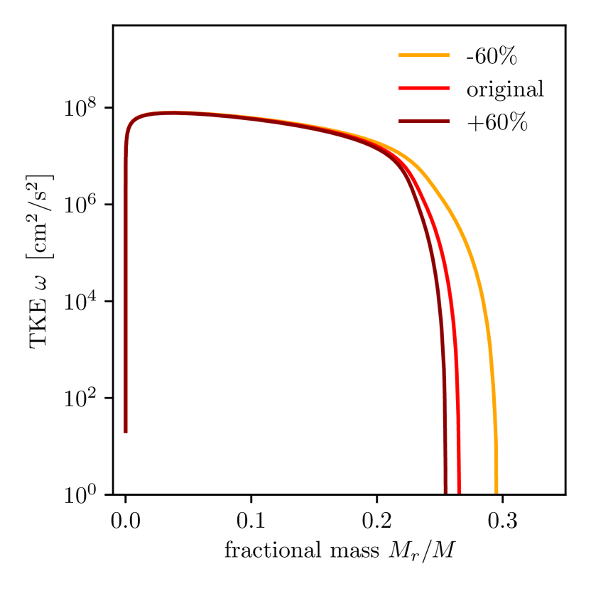
Figure 12: Comparison of the TKE as a function of fractional mass on a logarithmic scale for different values for the parameter $c_{4}$ in a 3-equation non-local $5\,M_{\odot}$ main-sequence model with limited dissipation length scale $\Lambda$.

Apart from the new parameters for the reduction of the dissipation length scale $\Lambda$, the model still contains the original parameters of the Kuhfuß model. Here, we focus on the parameter $\alpha_{\omega}$ which controls the flux of the TKE. In the 1-equation non-local model, this parameter controls the extent of the overshooting region. Kuhfuß suggested a default value of $\alpha_{\omega}=0.25$. In Fig. 13 we show three different hydrogen profiles for the $5\,M_{\odot}$ model at the same age. The parameter $\alpha_{\omega}$ takes values of 0.1, 0.3 and 0.5. It can be clearly seen that the original property of this parameter of controlling the overshooting extent is still given.

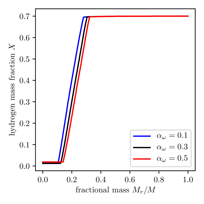
Figure 13: Comparison of the hydrogen profiles as a function of fractional mass for different values for the parameter $\alpha_{\omega}$ in a 3-equation non-local $5\,M_{\odot}$ main-sequence model with limited dissipation length scale $\Lambda$.

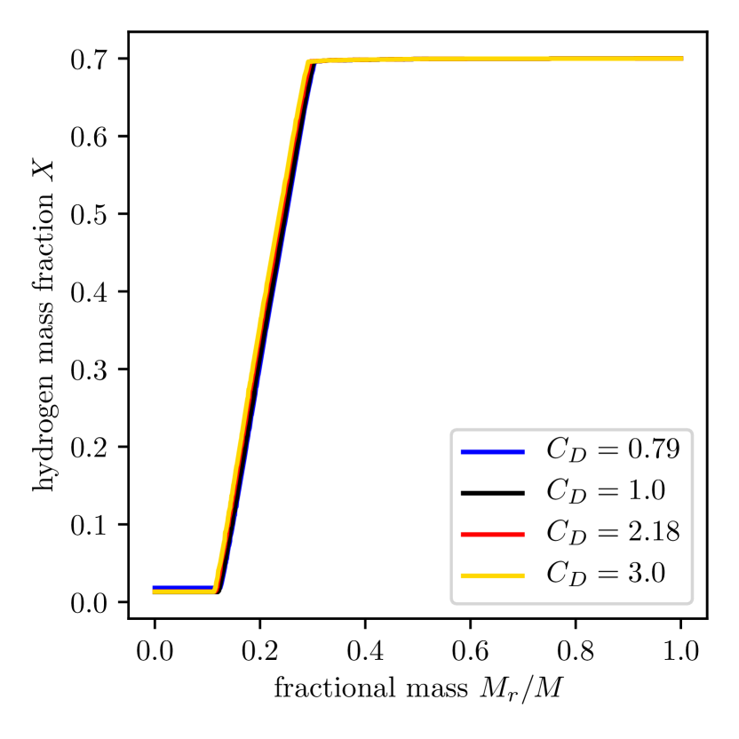
Figure 14: Comparison of the hydrogen profiles as a function of fractional mass for different values for the parameter $C_{\text{D}}$ in a 3-equation non-local $5\,M_{\odot}$ main-sequence model with limited dissipation length scale $\Lambda$.

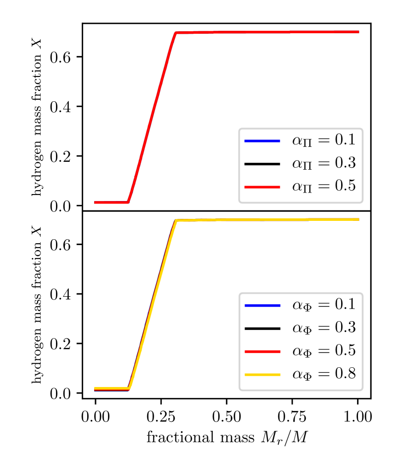
Figure 15: Comparison of the hydrogen profiles as a function of fractional mass for different values for the parameters $\alpha_{\Pi}$ and $\alpha_{\Phi}$ in a 3-equation non-local $5\,M_{\odot}$ main-sequence model with limited dissipation length scale $\Lambda$.

In Fig. 14 we show hydrogen profiles of a $5\,M_{\odot}$ star at the end of the main-sequence for different values of the dissipation parameter $C_{\text{D}}=0.79,1,2.18$ and 3. We always assume $C_{\text{D}}=c_{\epsilon}$, as both parameters have the same role in the Canuto & Dubovikov (1998) and in the Kuhfuß model. Here, the value of 0.79 refers to the default dissipation parameter from the Canuto & Dubovikov (1998) model, while 2.18 is the numerical default value in the Kuhfuß model. The extent of the hydrogen profile is largest for the model computed with the smallest dissipation parameter and smallest for the largest parameter. This behaviour is expected, as a decreased dissipation allows the TKE flux to extend further out. Compared to the parameter of the TKE flux $\alpha_{\omega}$, the impact of the dissipation parameter on the overshooting extent is rather limited, as the variation is much smaller when compared to the results shown in Fig. 13. The variation of the overshooting extent is also smaller, as one could have expected from the comparison shown in Fig. 12. This is because by changing $C_{\text{D}}$ also $c_{4}$ will change, while in Fig. 12 only $c_{4}$ is changed. The effects of changing $c_{4}$ and $C_{\text{D}}$ partially compensate each other, resulting in a smaller net effect. Finally, one could find combinations of parameters $\alpha_{\omega}$ and $C_{\text{D}}$ which allow obtaining models with equal convective core sizes. In Fig. 15 we show the impact of the parameter $\alpha_{\Pi}$ and $\alpha_{\Phi}$ in the upper and lower panel, respectively. They both have a negligible impact on the overshooting distance, which is yet smaller than the impact of the dissipation parameter $C_{D}$. This indicates again that the parameter $\alpha_{\omega}$ which determines the importance of the TKE flux has the largest impact on the overshooting distance (note that Fig. 12 has a different scale for the fractional mass axis).

Appendix C Ad hoc overshooting for small convective cores

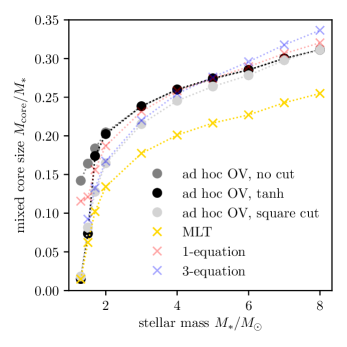
Figure 16: Comparison of mixed core sizes obtained with different descriptions of convection and different geometric cut to limit the overshooting (OV) for small cores in the ad hoc overshooting model.

Parametrised descriptions of overshooting like the diffusive or step overshooting use the pressure scale-height at the Schwarzschild boundary to define the overshooting distance. In the description of Freytag et al. (1996) the diffusion coefficient is computed according to:

$$D_{\rm adhoc}=D_{0}\exp\left(\frac{-2z}{f_{\rm OV}H_{p}}\right)$$ (13)

where $f_{\rm OV}$ is an adjustable parameter and $z$ is the radial distance to the Schwarzschild boundary. The pressure scale-height is, however, diverging towards the stellar centre. Hence, the inferred overshooting distance for a fixed overshooting parameter will increase for a decreasing convective size as well as the size of the mixed region. The resulting mixed core sizes for a fixed parameter value have been shown to be too large when comparing to observations (Pietrinferni et al. 2004; Magic et al. 2010). To avoid the unphysical growth of the overshooting region, the overshooting parameter needs to be artificially restricted. In GARSTEC the unphysical growth of the overshooting zone is prevented by comparing the size of the Schwarzschild core to the pressure scale height and use the smaller one as the relevant length-scale. As usual, there are different ways to implement this. Originally, Magic et al. (2010) suggested the following expression:

$$\widetilde{H_{p}}=H_{p}\cdot\mathrm{min}\left(1,\left(\frac{r_{\mathrm{CZ}}}{H_{p}}\right)^{2}\right)$$

where $r_{\mathrm{CZ}}$ is the radius of the Schwarzschild boundary. A correction factor of the same type was also used in Higl et al. (2021) when comparing GARSTEC results to 2D simulations, while introducing a factor of 2 in the denominator:

$$\widetilde{H_{p}}=H_{p}\cdot\mathrm{min}\left(1,\left(\frac{r_{\mathrm{CZ}}}{2H_{p}}\right)^{2}\right)$$ (14)

As the size of the convective core is now compared to a length scale twice as large as the original expression the size of the overshooting region is limited more strongly by the latter expression. The comparison to 2D simulations (Higl et al. 2021) as well as the study of the eclipsing binary TZ For (Higl et al. 2018) revealed, however, that this expression is finally limiting the size of the convective core too strongly. This led to the introduction of a different functional form of the limitation:

$$\widetilde{H_{p}}=H_{p}\cdot\mathrm{min}\left(1,\frac{1}{2}\left[\mathrm{tanh}\left(5\left(\frac{r_{\mathrm{CZ}}}{H_{p}}-1\right)\right)+1\right]\right)$$ (15)

which is less strongly limiting the core sizes at $2\,M_{\odot}$ but very quickly limiting the size of the mixed cores for smaller masses.

In Fig. 16 we show a comparison of the mixed core sizes obtained without any cut, with the square cut according to Eq. (14) and with the tanh cut according to Eq. (15). For reference, results obtained with MLT and the 1- and 3-equation models are shown in the same figure. As discussed above, the square cut is more restrictive than the tanh cut at masses around and above $2\,M_{\odot}$. Only at a mass of $8\,M_{\odot}$ the square cut does not restrict the convective core size any more. In contrast, the tanh cut restricts the core size only marginally, already at $2\,M_{\odot}$. For lower masses below about $4\,M_{\odot}$, the results of the square cut are in good agreement with the 3-equation model.