Constraining the Charge-, Time- and Rigidity-Dependence of Cosmic-Ray Solar Modulation with AMS-02 Observations during Solar Cycle 24

Abstract

Our basic theoretical understanding of the sources of cosmic rays and their propagation through the interstellar medium is hindered by the Sun, that through the solar wind affects the observed cosmic-ray spectra. This effect is known as solar modulation. Recently released cosmic-ray observations from the Alpha Magnetic Spectrometer (AMS-02) and publicly available measurements of the solar wind properties from the Advanced Composition Explorer and the Wilcox observatory allow us to test the analytical modeling of the time-, charge- and rigidity-dependence of solar modulation. We rely on associating measurements on the local heliospheric magnetic field and the heliospheric current sheet’s tilt angle, to model the time-dependence and amplitude of cosmic-ray solar modulation. We find evidence for the solar modulation’s charge- and rigidity-dependence during the era of solar cycle 24. Our analytic prescription to model solar modulation can explain well the large-scale time-evolution of positively charged cosmic-ray fluxes in the range of rigidities from 1 to 10 GV. We also find that cosmic-ray electron fluxes measured during the first years of cycle 24 are less trivial to explain, due to the complex and rapidly evolving structure of the Heliosphere’s magnetic field that they experienced as they propagated inwards.

I Introduction

The Sun produces a time-varying stream of charged particles known as the solar wind that extends out to at least 100 astronomical units (AU). This region is called the Heliosphere. The solar wind and its embedded magnetic field known as Heliospheric Magnetic Field (HMF) can have a strong effect on cosmic rays entering from the interstellar medium (ISM), the space outside the Heliosphere and between stellar systems in our Galaxy. Cosmic rays propagating through the Heliosphere get deflected and lose energy by interacting with the HMF. As the HMF changes with time its effect on the observed cosmic-ray spectra at Earth has an imprinted time-variation Usoskin et al. (2011); Caballero-Lopez and Moraal (2012); Corti et al. (2019, 2020); Burger et al. (2022). This effect is known as solar modulation of cosmic rays. With current cosmic-ray observations Aguilar et al. (2013); Adriani et al. (2016); Abe et al. (2017) the statistical errors associated with the detected fluxes are now much smaller than the systematic uncertainties associated with cosmic-ray propagation, including solar modulation. Given this high precision era for cosmic rays, it is important to properly understand how the Sun influences these spectra in order to make reliable inferences on how cosmic rays are produced and propagate throughout the Milky Way Kachelriess et al. (2011); Cholis and Hooper (2014); Hooper et al. (2015); Mertsch and Sarkar (2014); Strong (2015); Kohri et al. (2016); Malkov et al. (2016); Cuoco et al. (2017); Cui et al. (2017); Cholis et al. (2017, 2018); Lowell et al. (2019); Kuhlen and Mertsch (2019); Engelbrecht and Di Felice (2020); Wang et al. (2019); Cholis et al. (2019); Cuoco et al. (2019); Heisig et al. (2020); Engelbrecht and Moloto (2021); Potgieter et al. (2021); Cholis and Krommydas (2022).

In this work, we follow a data-driven approach where we test the analytic model of Cholis et al. (2016) to cosmic-ray measurements. This analytic model includes to first order the effects of cosmic-ray diffusion experienced through different regions of the Heliosphere and the presence of drift effects (see also Gieseler et al. (2017); Aslam et al. (2019); Corti et al. (2019); Kuhlen and Mertsch (2019); Vittino et al. (2019)). To include the time-evolution of the HMF and its impact on solar modulation, we use ongoing observations from the Advanced Composition Explorer’s (ACE) Smith et al. (1998); http://www.srl.caltech.edu/ACE/ASC/ magnetometer and the Solar Wind Electron Proton Alpha Monitor (SWEPAM) https://izw1.caltech.edu/ACE/ASC/level2/swepam_l2 desc.html . We also use information on the value of the tilt angle of the heliospheric current sheet (HCS) -associated to the time-varying morphology of the HMF- from publicly available model-parameters provided by the Wilcox Solar Observatory (WSO) http://wso.stanford.edu/Tilts.html . We have found that the tilt angle of the heliospheric current sheet (HCS) and the magnitude of the HMF measured at the position of Earth have a strong correlation to the cosmic-ray solar modulation and are well observed using ACE data and the WSO. However, we do not find a strong correlation to the solar wind’s bulk speed essentially considering it fixed in time, while it still has a radial dependence Heber and Potgieter (2006).

As particles enter the Heliosphere they are deflected through the magnetic field. For a given solar magnetic polarity $A$ of the HMF, depending on its charge $q$ a cosmic ray particle is more likely to reach the Earth by propagating through different regions of the Heliosphere. When the combination of $qA<$ 0, particles propagate mostly through the HCS, while when $qA>$ 0, particles propagate mostly through the solar magnetic poles Jokipii and Thomas (1981); Kota and Jokipii (1983); Caballero-Lopez and Moraal (2004); Potgieter (2013, 2014, 2017). Moreover, particles that propagate through the HCS travel slower compared to particles traveling through the magnetic poles with the same magnitude of rigidity $|R|=p/|q|$ (where $p$ is the particle’s momentum and $q$ its charge). This results in larger energy losses for the former particles on average and thus a more significant change in their observed intensity and energy. In our work, we model the averaged effect of the different paths that cosmic rays of opposite charge follow as they propagate to the Earth. We note that this assumption effectively breaks the spherical symmetry that conventional force field models assume for the solar modulation Gleeson and Axford (1968). Extensive numerical works have also explored this break away from 1-dimensional propagation Caballero-Lopez and Moraal (2004); Strauss et al. (2012); Qin and Shen (2017); Boschini et al. (2018); Jerome Boschini et al. (2019); Caballero-Lopez et al. (2019); Bisschoff et al. (2019). However, as we will describe in detail we retain the force field notation as it gives a simple qualitative description of the impact the HMF has on the cosmic-ray spectra measured at Earth versus those in the local ISM.

This paper is organized as follows; in Section II we present the observations we use to model the time-varying HMF properties and also the cosmic-ray spectra that we rely on. In Section III, we present the analytic model for the solar modulation that we test to the cosmic-ray measurements. In Section IV, we present our results finding that indeed there is a clear indication in the cosmic-ray data of a charge dependence on the solar modulation. Our charge-, time- and rigidity-dependent model can explain well the larger-scale time-evolution of positively charged cosmic-rays (hydrogen and positrons) in the range of rigidities from 1 to 10 GV. We can also explain some of the observations of electrons in the same rigidity range and time, especially once we find that cosmic-rays experience a stable Heliospheric polarity as they propagate inwards. Finally, in Section V we present our conclusions and discuss the remaining open questions and further directions on the modeling of the time-varying, change- and rigidity-dependent effects of solar modulation.

II Data

This paper covers observations made during solar cycle 24, and in particular we focus on the era from Bartels’ rotation (BR) cycle 2456 to Bartels’ rotation cycle 2506 (roughly August 2013 to April 2017). During this era, the properties of the HMF have been extensively studied and measured. It represents also a time interval during which the polarity of the HMF is well defined to be positive ($A>0$). In Fig. 1, the amplitude of the HMF $|B_{tot}|$, measured at the Earth’s location (at 1 AU), the tilt angle $\alpha$, and the solar wind’s bulk speed measured also at 1 AU are plotted as they change over time. While the strength of the magnetic field and the bulk speed are directly measured by the ACE instruments, the plotted tilt angle gives the maximum extent in latitude reached by the computed HCS, i.e. describes the general structure of the HMF. This is a model-dependent result , relying on observations of the solar magnetic field. The time-varying tilt angle information is publicly available from the WSO http://wso.stanford.edu/Tilts.html ; Hoeksema (1992); Ferreira and Potgieter (2004). To first order the bulk wind speed time-variation is very mild and from here on its time-dependence is ignored. We concentrate on the HMF’s $|B_{tot}|$ and $\alpha$ quantities, in agreement with earlier works Cholis et al. (2016, 2020).

Figure 1: The amplitude of the solar magnetic field $|B_{tot}|$, measured at 1 AU (solid black) with axis units and range information on the left $y$-axis. Also plotted are the solar wind bulk speed at 1 AU (blue dashed-doted line) with its units and range also on the left $y$-axis and the tilt angle of the current sheet (red dashed line and right $y$-axis).

We use cosmic-ray observations made by the Alpha Magnetic Spectrometer (AMS-02) to fit the model parameters of Ref. Cholis et al. (2016). In particular, we use the cosmic-ray hydrogen (proton plus deuteron) spectra taken from 2013 to 2017, between BR 2456 and BR 2506 Aguilar et al. (2018a) and the equivalent period for electron and positron cosmic-ray spectra Aguilar et al. (2018b). These observations by AMS-02 allow us to model changes between Bartels’ rotation cycles in the respective cosmic-ray fluxes i.e. changes that appear over 27-day long time scales. Moreover, to study the rigidity-dependence of solar modulation, we use observations over five separate rigidity ranges. Those span the ranges of 1.16-1.33, 1.92-2.15, 3.29-3.64, 5.37-5.90, and 9.26-10.1 GV. We do not expand our analysis to higher rigidities as the respective solar modulation changes between BRs are too small. Once studying the observations of that era we noticed that the cosmic-ray fluxes fluctuate roughly around the same average over the first half of 2013-2017 era, while after that all fluxes increase nearly monotonically. For that reason, we break our analysis in two sub-eras, the first one being from BR 2456 to BR 2481 and the second from BR 2482 to BR 2506. Since we care about the evolution of the fluxes, we follow Ref. Cholis et al. (2020), where it was shown that in order to reduce the impact of ISM assumptions, it is best to study the evolution of the fluxes around their respective averaged flux. This still allows us to focus on the relative changes of the hydrogen, electron and positron fluxes over time. We also note that at lower rigidities the time evolution of the cosmic-ray hydrogen flux -and thus also its ratio to the averaged observed flux- is significantly more prominent. At the 1.16-1.33 GV bin the time variation is at the $-50\%\;+80\%$ level for the entire 2013-2017 era, while at the 9.26-10.1 GV bin it is at the $\pm 5\%$ level.

III Methodology

The analytic treatment of solar modulation that we employ follows Cholis et al. (2016), where the force-field approximation was expanded to include a time-, charge- and rigidity-dependence on the solar modulation. The effect of solar modulation like in Gleeson and Axford (1968), is that the kinetic energy $E_{kin}$ of each particle is reduced on average by $|Z|e\Phi$, where $\Phi$ is the modulation potential, generally on the order of 0.1 - 1.0 GV, and $|Z|e$ is the absolute charge of the cosmic ray. The resulting effect of the modulation potential on the cosmic-ray differential spectrum can be written as:

$$\frac{dN^{\oplus}}{dE_{kin}}(E_{kin}) = \frac{(E_{kin}+m)^{2}-m^{2}}{(E_{kin}+m+|Z|e\Phi)^{2}-m^{2}}$$ (1)

$$\times \frac{dN^{ISM}}{dE_{kin}}(E_{kin}+|Z|e\Phi)$$

where $E_{kin}$ is the observed kinetic energy and the subscripts “$ISM$" and “$\oplus$" denote the respective values in the local interstellar medium and at the location of Earth. In the standard force field approach, the value of $\Phi$ is fitted to the cosmic-ray observations without a prediction on what its value should be at any given time nor accounting for the fact that particles of opposite charge propagate through different regions of the Heliosphere. Moreover, the value of $\Phi$ is assumed to be the same for all cosmic rays irrespective of the energy they carry as they enter the HMF. In this work we instead follow Cholis et al. (2016), where the solar modulation potential depends on three well-studied quantities: the polarity of the solar magnetic field, the magnitude of the HMF at 1 AU, and the tilt angle of the HCS. The analytic expression for the solar modulation potential is as follows:

$$\Phi(R,q,t) = \phi_{0}\left(\frac{|B_{tot}(t)|}{4nT}\right)$$ (2)

$$+ \phi_{1}H(-qA(t))\left(\frac{|B_{tot}(t)|}{4nT}\right)$$

$$\times \left(\frac{1+(\frac{R}{R_{0}})^{2}}{\beta(\frac{R}{R_{0}})^{3}}\right)\left(\frac{\alpha(t)}{\frac{\pi}{2}}\right)^{4}.$$

$A$ is the polarity of the HMF and $|B_{tot}|$ its strength as measured at Earth. $\alpha$ is the tilt angle of the HCS. These quantities are considered time-dependent inputs, and therefore independent of cosmic-ray observables. $R$, $\beta$, and $q$ are the rigidity, velocity/$c$, and charge of the cosmic ray, respectively. $H$ is the Heaviside step function separating the treatment of opposite charges cosmic rays based on the product of $q$ and $A$ as in Figure 1 of Cholis et al. (2016). $R_{0}$ is a reference rigidity at which point drift effects are important along the HCS and $\phi_{0}$ and $\phi_{1}$ are normalization factors fitted to the data that represent the amplitude of the combined effect of diffusion and drift. To test our solar modulation model to cosmic-ray measurements conducted at different times we use AMS-02 data from Refs. Aguilar et al. (2018a, b), as described in Section II. We constrain the parameters of $\phi_{0}$, $\phi_{1}$ and $R_{0}$ by fitting them to the available cosmic-ray data for solar cycle 24.

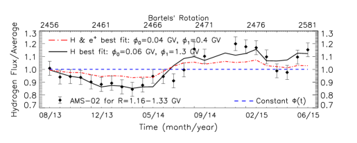
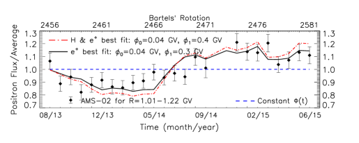
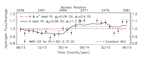
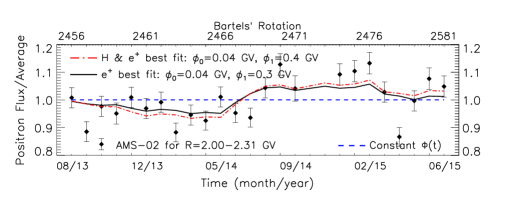
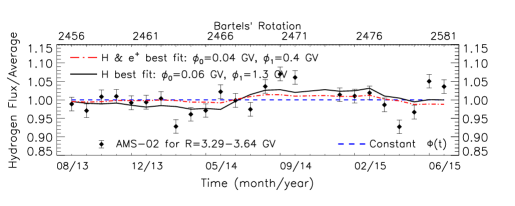
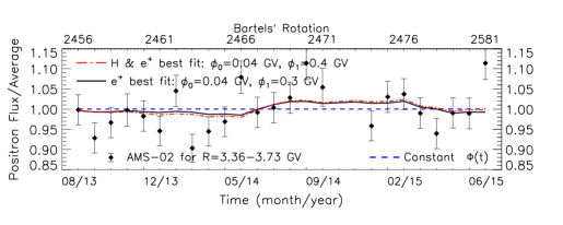
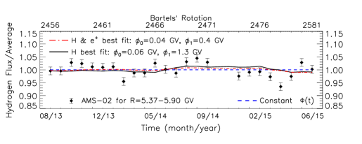
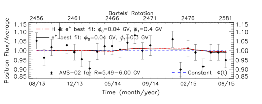
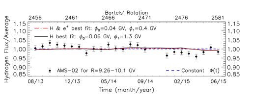
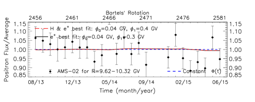
Figure 2: Left column: the time evolution of the ratio of the cosmic-ray hydrogen flux to the averaged hydrogen cosmic-ray flux within a period of the 24 observed Bartel’s cycles (BR 2456-2481). We show the following five rigidity bins, from top to bottom: 1.16-1.33, 1.92-2.15, 3.29-3.64, 5.37-5.90, 9.26-10.1 GV. The error-bars come from the AMS-02 observations (see text for details), while the black line gives the best fit choice for the hydrogen (H) ratio for $\phi_{0}=0.06$ GV, $\phi_{1}=1.3$ GV and assuming $R_{0}=0.5$ GV. Right column: the time evolution of the ratio of the cosmic-ray positron flux to the averaged positron cosmic-ray flux within the same period of the 24 observed Bartel’s cycles. The rigidity bins used are not identical to the hydrogen ones as the rigidity binning performed by AMS-02 is not the same for the two cosmic-ray species. We used the closest possible positron rigidity bins of 1.01-1.22, 2.00-2.31, 3.36-3.73, 5.49-6.00, 9.62-10.32 GV. The black line gives the best fit choice for the positron ($e^{+}$) ratio for $\phi_{0}=0.04$ GV, $\phi_{1}=0.3$ GV and assuming $R_{0}=1.0$ GV. The red dashed-dotted lines on both the left and right columns give the evolution of the respective hydrogen and positron flux ratios as predicted for values of $\phi_{0}=0.04$ GV and $\phi_{1}=0.4$ GV. These values give the best fit to the combination of the positively charged cosmic-ray particles used for that era (see text for further details).

We perform a $\chi^{2}$ test to get the best fit values of the parameters, $\phi_{0}$, $\phi_{1}$ and $R_{0}$. This parameter space is probed through a discrete grid that was found to give smoothly changing $\chi^{2}$ values. For each combination of $\phi_{0}$, $\phi_{1}$ and $R_{0}$ values, the solar modulation function is calculated for every Bartels’ cycle, once for protons and once for deuterons. The resultant fluxes of protons and deuterons are added to get a value for the hydrogen flux at each Bartels’ cycle. The hydrogen fluxes over the 24 Bartels’ cycles of BR 2456 to 2581 are averaged for each of the five rigidity bins of 1.16-1.33, 1.92-2.15, 3.29-3.64, 5.37-5.90, and 9.26-10.1 GV. Then, the value for the hydrogen flux at each Bartels’ cycles is divided by the average hydrogen flux, resulting in a list of 24 hydrogen flux ratios, that act as the “expected” values of hydrogen flux ratio for the given parameter values. Each of those ratios has an uncertainty that is directly proportional to the reported AMS-02 flux uncertainty (statistical and systematic added in quadrature) for the given Bartels’ cycle. Those ratios and respective uncertainties are represented by the “AMS-02” data with error-bars in Fig. 2 in the left column for the hydrogen flux ratio (“Hydrogen Flux/Average”). We repeat the same procedure for positrons (shown in Fig. 2 right column), as well as electrons for BR 2456-2481 and again for the hydrogen, positron and electron observations of the era between BR 2482 and BR 2506 as we describe in in Section IV.

By taking the ratio of the cosmic-ray hydrogen or positron or electron fluxes at different Bartels’ rotations over their respective average we find that some of the underlying systematic modeling uncertainties of the ISM fluxes cancel out, allowing us for a more direct test of solar modulation (see also Cholis et al. (2020)). Moreover, the local cosmic-ray ISM fluxes in that range of rigidities i.e. 1-10 GV are stable on timescales of order $O(10)$ Myr allowing only for the solar modulation to cause any changes. In fact, even at rigidities as high as TVs, local sources such as pulsars or recent supernova remnants can have an effect on the spectra on a timescale of only $O(10^{4})$ years (see e.g. Profumo (2011); Cholis and Hooper (2014); Mertsch and Sarkar (2014); Cholis et al. (2017, 2018); Mertsch (2018); Cholis and Krommydas (2022)).

The standard $\chi^{2}$ test is performed, comparing the list of “expected” hydrogen, or positron, or electron flux ratios to the observed cosmic-ray spectra from AMS-02, summing up the value for every Bartels’ cycle to get the overall $\chi^{2}$ value.

For the predicted local ISM fluxes we used the predictions of model “C” from Cholis et al. (2022) for the protons and deuterons. These ISM assumptions were found to give cosmic-ray fluxes in agreement with the hydrogen, helium, and carbon fluxes as well as boron-to-carbon, carbon-to-oxygen and beryllium-to-carbon flux ratios measured by AMS-02 at the entirety of the energies not affected by solar modulation. These cosmic-ray spectra have been evaluated by running the publicly available GALPROP code Strong and Moskalenko (1998); http://galprop.stanford.edu ; of GALPROP availabe at: https://galprop.stanford.edu/code.php . In addition, the local ISM positron and electron fluxes come from Cholis and Krommydas (2022) (“Model I”) that relies on the ISM assumptions of model “C” from Cholis et al. (2022) for the calculation of primary and secondary cosmic-ray electron and positron fluxes and, through the presence of local pulsars, further explains the cosmic-ray positron fraction ($e^{+}/(e^{+}+e^{-})$) spectrum, cosmic-ray positron, cosmic-ray electron plus positron flux observations from AMS-02 and from the Dark Matter Particle Explorer (DAMPE) and the CALorimetric Electron Telescope (CALET) Aguilar et al. (2019a, b, 2021); Ambrosi et al. (2017); Adriani et al. (2018).

IV Results

Positively charged particles during cycle 24 mostly probe the parameter $\phi_{0}$, as during that time $A>0$ and they propagate to the Earth through the heliospheric poles. Conversely, negatively charged particles probe the $\phi_{1}$ and $R_{0}$ parameters as well. That can be seen in Eq. 2 through its switching off or on of the second term on the total modulation potential $\Phi(R,q,t)$. For that reason, we test the time evolution of the cosmic-ray hydrogen, positron and electron fluxes. Yet, that statement is accurate only for the case where the observed cosmic-rays measured at Earth propagated through the Heliosphere while the polarity of the HMF was well established. This is important as from simulations (see e.g. Ref. Strauss et al. (2012)) we understand that cosmic-ray particles may take approximately a year for them to propagate through the $\simeq 100$ AU of distance to reach the AMS-02 detectors. Moreover, given the bulk speed of the outward moving solar wind, it takes in addition half a year to a year for the HMF new polarity to be established all the way to the edge of the Heliosphere. Thus, even if the HMF polarity $A$ flip is instantaneous at the Sun, cosmic-ray particles reaching the Earth two years after that moment may have experienced a non-well defined HMF polarity during their inward propagation. There is a significant time-delay between HMF changes observed at the surface of the Sun or at 1 AU and their effect on cosmic-ray fluxes through solar modulation. In Ref. Cholis et al. (2020), that time delay was estimated to be $\simeq 20$ months even when studying observations made at the end of solar cycle 23 before the change of HMF from $A<0$ to $A>0$. In our case that time-delay may be even larger especially since the polarity flip was not instantaneous. Based on observations reported by the WSO, the most likely moment of the polarity flip was May of 2013. However, the Sun’s 30-day window averaged polar field measurements between October 2012 and March 2014 as reported in http://wso.stanford.edu/Polar.html suggest that the polarity flip of the Sun’s field was not instantaneous.

Originally we started to study data from BR 2453 onwards (May 2013) and averaged the entire era of BR 2453 to BR 2506 when the AMS-02 observations of Refs. Aguilar et al. (2018a, b) end . We noticed two important points. One, it is very difficult to explain the entirely of that time with any simple model dependent on the polarity, tilt angle, total magnetic field or bulk speed observations. Moreover, the first months are too close to the polarity flip to be a useful to understanding the overall propagation of cosmic rays through the Heliosphere. Simply put, those cosmic rays as they were approaching the Earth experienced a significant field change towards the end of their path.

We chose to focus on the data from BR 2456 onwards. In addition, we break the data into two sections of equal time intervals of BR 2456-2481 when the effect of a non-well defined polarity experienced by the inward propagated observed cosmic rays suggests the presence of both the $\phi_{0}$ and $\phi_{1}$ terms of Eq. 2 on positively and negatively charged particles. However, for BR 2482-2506, positively charged particles experience a monotonic turning-off the $\phi_{1}$-term which completely shuts down at BR 2490. This is in agreement with the long time delay between the polarity change on the Sun’s surface and its effect on the observed cosmic rays. For the eras that we study, we provide in Fig. 3, the averaged HMF magnetic field amplitude (using its value at 1 AU as a probe for time-evolution in the Heliosphere) and tilt angle that the cosmic rays experience. As can be seen small timescale effects of Fig. 1 are washed out.

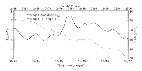
Figure 3: Time evolution of the averaged HMF properties that cosmic rays at Earth have experienced.

For particles arriving at Earth up to BR 2481 we took the same averaging assumptions as in Ref. Cholis et al. (2020). That is the $B_{\rm tot}(t)$ is averaged over 4 BRs with a time delay of 16 BRs. i.e. for positively charged particles arriving at BR 2456 we evaluate $B_{\rm tot}(t)$ of Eq. 2 using the ACE observations of BR 2437-2441. For the $\alpha(t)$ we use instead the averaged value of the last 20 BRs, without any further time-delay, i.e. in the specific example the WSO modeled predictions for $\alpha$ between BR 2437-2456. These choices where shown to provide the best fit to the AMS-02 observations of positively charged particles traveling through the HCS and are true even for the first Bartels’ rotations with the new solar cycle. We did confirm that by testing alternative averaging choices and came to the same conclusions as in Cholis et al. (2020). For later Bartels’ rotations, instead these same particles traveled through the Heliospheric poles; thus traveling faster to the Earth. Thus their averaging scheme is expected to be shorter (see e.g. Strauss et al. (2012); Potgieter (2013)). In Table 1 we give the assumptions that we tested for the positively charged particles for the period where we expect that cosmic rays propagated inwards through the poles. We used the era of BR-2482-2506. We report the difference in the $\chi^{2}$ fit of the five rigidity bins for the hydrogen data that we use ($\Delta\chi^{2}$), between the best choice and alternative ones. The best fit choice is achieved with an averaging scheme where both $B_{\rm tot}(t)$ and $\alpha(t)$ are averaged over 4 BRs with zero time delay. That is, for a positively charged particle that arrived at BR 2500 the evaluated $B_{\rm tot}(t)$ and $\alpha(t)$ of Eq. 2, used the ACE and WSO averaged observations of BR 2497-2500. We report the hydrogen data for simplicity as those have the most statistical weight. However, the same conclusions are derived if we use the combination of hydrogen and positrons.

$B_{\rm tot}(t)$	$B_{\rm tot}(t)$	$\alpha(t)$	$\alpha(t)$	$\Delta\chi^{2}$
time aver.	time delay	time aver.	time delay	from
($\#$BR)	($\#$BR)	($\#$BR)	($\#$BR)	best fit
4	4	0	0	–
4	4	1	1	118
4	4	2	2	182
4	4	4	4	245
9	9	0	0	1639
9	9	1	1	1734
6	6	0	0	1866
12	12	0	0	1912
1	1	0	0	1968

Table 1: A sample of time averaging schemes for the values of $B_{\rm tot}$ and $\alpha$, that the positively charged particles experience. We give the corresponding $\Delta\chi^{2}$ from the best fit choice relying on the AMS-02 hydrogen observations (see text for details).

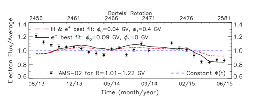
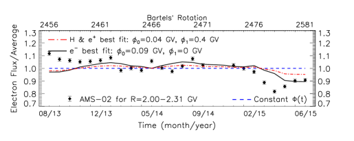
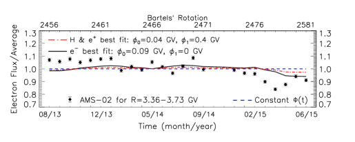
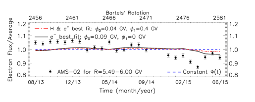
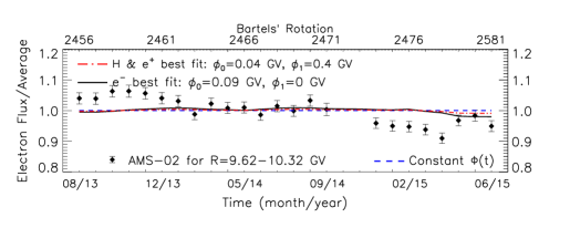
Figure 4: Time evolution of the ratio of cosmic-ray electron flux to the averaged electron cosmic-ray flux within a period of Bartels’ cycles 2456 and 2481. We show the same five rigidity bins as for positrons (see right column of Fig. 2), from top to bottom: 1.01-1.22, 2.00-2.31, 3.36-3.73, 5.49-6.00, 9.62-10.32 GV. The solid black line gives the best fit choice for electrons derived for $\phi_{0}=0.09$ GV, $\phi_{1}=0$ GV and $R_{0}=0.05$ GV (see text for details). The red dashed-dotted lines give the prediction for the evolution of the electron flux ratio using $\phi_{0}=0.04$ GV and $\phi_{1}=0.4$ GV that were derived to give the best fit to the combination of the positively charged cosmic-ray particles in the same era (see text for further details).

As we wrote, the hydrogen and positron cosmic-ray spectra constrain the values of $\phi_{1}$ and $R_{0}$ as well. We find that $\phi_{1}>0$ is clearly preferred by the data even for the positively changed particles. This provides a clear indication for the charge-dependence of solar modulation on cosmic rays. In Fig. 2, both the hydrogen and the positron flux ratios general time evolution for BR 2456-2481 can be described through a value of $\phi_{0}\sim 0.05$ GV and a $\phi_{1}\geq 0.3$. The respective black lines provide the best fit to the five rigidity bins and 24 BR data points . The red-dashed dotted lines instead assume that both hydrogen’s and positrons’ solar modulation is described by the same combination of $\phi_{0},\;\phi_{1}$ parameters. The best fit values for the combination of these species’ flux evolution is $\phi_{0}=0.04$ GV and $\phi_{1}=0.4$ GV. The lines on the left and right are not identical due to the different masses of these particles. The time evolution of the hydrogen and positron fluxes are most prominent in the lowest two rigidity bins and present also in the bin around 3.5 GV. For rigidities above 5 GV while there are still statistically significant time-variations especially for the hydrogen flux, the time-patterns observed at low rigidities are not present. In addition, our fitted model suggests very marginal time-evolution for the flux ratios at these higher rigidities. In Fig. 2, we provide a blue dashed line that represents the effect of non-zero but also constant in time solar modulation potential $\Phi$.

Our model does explain well the general time-evolution of solar modulation. This demonstrates that a simple analytic formula can explain the AMS-02 observations and connect the solar modulation of different cosmic-ray species to directly observable quantities of the HMF. However, statistically our best fits never approach a $\chi^{2}$ per degree of freedom of approximately 1 that would suggest a proper good fit. At the higher rigidities there are specific Bartels’ cycles that deviate significantly from the observed averaged modulation (blue dashed lines), and our model can not explain these short timescale observations. Such examples are BR 2457, BR 2463 and BR 2478. These are times that the incoming cosmic rays were more strongly affected by the HMF structure than our time-averaged assumptions predict; as we systematically under-predict the resulting total modulation potential value $\Phi$. There are however cycles like BR 2475 where at one rigidity bin the flux decreased compared to the neighboring in time Bartels’ cycles and in the next rigidity bins it is increased. We believe that this indicates the level of stochasticity that solar modulation on the observed spectra is expected to have, and that is associated to the random paths of inwardly propagating cosmic-rays (see also Vittino et al. (2019)).

In Fig. 4, we give the time evolution of the cosmic-ray electron flux ratio over BR 2456 to BR 2481. During that era the $\phi_{1}$ term was mostly shut off for electrons. Thus, the $\phi_{1}=0$ and $R_{0}=0.05$ best fit values while still statistically significant due to the small size of the AMS-02 error-bars do not necessarily exclude other ranges for the $\phi_{1}$ and $R_{0}$ combination as we will explain later. We note however, that the electrons observations are not well explained by either our best fit parameters (black lines) nor the choice of $\phi_{0}=0.04$ GV and $\phi_{1}=0.4$ GV that explain the combination of the positively charged particles in the same era (red dashed-dotted lines in Fig. 4). In fact, the electron data of that era provide the greatest challenge of any species/era in our work. The issues we experience are beyond a small number of unique Bartels’ rotation cycles. Also, our model under-predicts the time evolution both at the lower and higher rigidity bins. Electrons seem to be the most affected by the polarity flip as with the $A<0$ before that flip they would have traveled to the Earth through the solar poles. Our model assumes that was still the case for most of the BR 2456 to BR 2481 era and the tension with the data, suggests that their path through the Heliosphere during that transitional era was more complex.

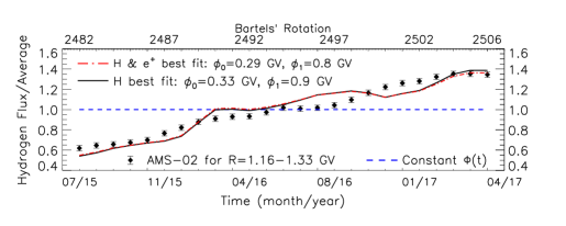
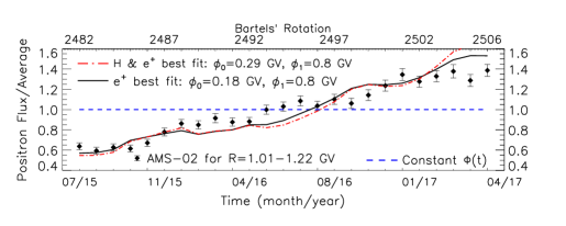
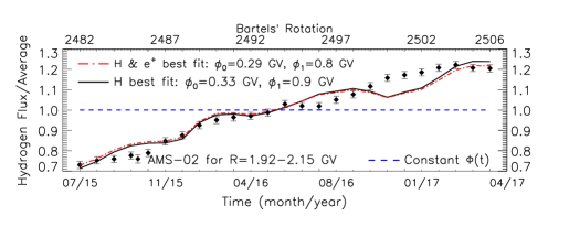
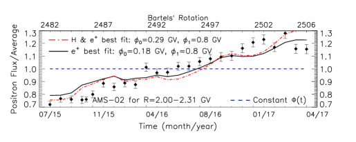
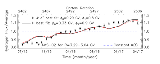
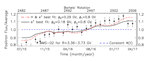
Figure 5: As with Fig. 2, for the 25 observed Bartel’s cycles of BR 2482-2506. Left column: the time evolution of the ratio of the cosmic-ray hydrogen flux to the averaged hydrogen cosmic-ray flux. We show the following three lower rigidity bins, from top to bottom: 1.16-1.33, 1.92-2.15 and 3.29-3.64 GV. The black line gives the best fit choice for the hydrogen (H) ratio for $\phi_{0}=0.33$ GV, $\phi_{1}=0.9$ GV and assuming $R_{0}=2$ GV. Right column: the time evolution of the ratio of the cosmic-ray positron flux to the averaged positron cosmic-ray flux for the era of study. We show the positron rigidity bins of 1.01-1.22, 2.00-2.31 and 3.36-3.73 GV. The black line gives the best fit choice for the positron ($e^{+}$) ratio for $\phi_{0}=0.18$ GV, $\phi_{1}=0.8$ GV assuming $R_{0}=1.0$ GV. The red dashed-dotted lines on both left and right columns give the evolution of the respective hydrogen and positron flux ratios as predicted for values of $\phi_{0}=0.29$ GV and $\phi_{1}=0.8$ GV, which provide the best fit to the combination of both particle species at that era (see text for details).

In Fig. 5, we plot the time-evolution for the positively charged particles during the BR 2482 to BR 2506 era. During that time the $\phi_{1}$ term of Eq. 2, gradually switched off for the positively charged particles, being present up to BR 2489. This choice is used to model the time it takes for positively charged particles’ trajectories to stabilize in reaching Earth through the Heliospheric poles. Any effect the AMS-02 data may have on $\phi_{1}$, $R_{0}$ parameters is solely dependent on the first eight (BR 2482-2489) data points. In Table 2, we show the impact alternative options on the switching off of the $\phi_{1}$ term have on the quality of the $\chi^{2}$-fit to the AMS-02 data. That switching off of the $\phi_{1}$ term, is based on the best-fit averaging choices for $B_{\rm tot}(t)$ and $\alpha(t)$, that we discussed earlier. For that era these are also given in Table 1.

From the BR 2482 to BR 2506 era, we find that fitting the hydrogen and positron flux ratio evolution independently or together has only a small effect on the derived modulation potential parameters. Hydrogen data require larger values of $\phi_{0}=0.33$ GV and $\phi_{0}=0.9$ GV compared to positrons, that give best fit for $\phi_{0}=0.18$ GV and $\phi_{0}=0.8$ GV. These are depicted by the respective black lines on the left and right columns of Fig. 5. Our results rely on the same five rigidity bins used for BR 2456 to BR 2481 of Fig. 2. However, as with that era the statistically most prominent rigidities are the lowest. The best-fit combination result for both positively charged cosmic-ray species is achieved for $\phi_{0}=0.29$ GV and $\phi_{0}=0.8$ GV, shown through the red dashed-dotted lines.

Last BR with $\phi_{1}$-term	First BR with $\phi_{1}$-term	$\Delta\chi^{2}$
fully switched on	switched off	from
($\#$BR)	($\#$BR)	best fit
2483	2490	–
2484	2491	21
2485	2491	40
2480	2503	60
2480	2501	63
2480	2500	76
2480	2499	88
2480	2497	116
2483	2494	162

Table 2: A variety of schemes for the switching off of the $\phi_{1}$ term of Eq. 2 with the corresponding $\Delta\chi^{2}$ from the best fit option (see text for details).

In Fig. 6, we show the evolution of the cosmic-ray electron flux between BR 2482 to 2506. Unlike the first era of study, our model describes the general trend of the electron flux increasing over time. We find that the best fit choice is achieved for a combination of $\phi_{0}=0.34$ GV, $\phi_{1}=0$ GV and $R_{0}=0.05$ GV (black solid line). However, even the assumptions from fitting the positively charged particles of the same era, i.e. $\phi_{0}=0.29$ GV, $\phi_{1}=0.8$ GV (red dashed-dotted lines), are in a similar level of agreement. In fact the $\phi_{1}$ parameter on electrons remains quite weakly constrained by the observations of that era. Yet, the overall quality of fit still remains poor. The main reason for this tension is that our model gives a greater level of electron flux variability with time over the studied period than the AMS-02 data suggest. Other averaging effects may be in play, associated likely to the stochastic nature of paths followed by individual cosmic-rays before reaching us. We leave that as a subject of future study, to be addressed with more observational data.

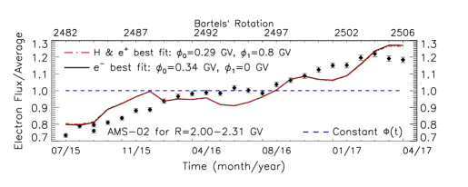
Figure 6: As with Fig. 4, for the 25 observed Bartel’s cycles of BR 2482-2506. We show the first three rigidity bins as for electrons, from top to bottom: 1.01-1.22, 2.00-2.31 and 3.36-3.73 GV. The solid black line gives the best fit choice for electrons derived for $\phi_{0}=0.34$ GV, $\phi_{1}=0$ GV and $R_{0}=0.05$ GV. The red dashed-dotted lines give the prediction for the evolution of the electron flux ratio using $\phi_{0}=0.29$ GV and $\phi_{1}=0.8$ GV that give the best fit to the combination of the positively charged cosmic-ray particles in the same era (see text for further details).

V Conclusions and Discussion

We conclude our work by presenting the $\phi_{0}$, $\phi_{1}$ projected space limits from all three types of cosmic rays; hydrogen (i.e. protons and deuterons), positrons and electrons. The 1-, 2- and 3-$\sigma$ acceptable ranges are given in Fig. 7. The hydrogen ratio ranges are provided with purple contours, while the positron ratio ranges are given by the blue contours. Finally, the electron ratio ranges are given by the orange contours.

In both eras there are combinations of $\phi_{0}$, $\phi_{1}$ values that can explain the observations from all three species, i.e. $\phi_{0}$, $\phi_{1}$ where all three contours overlap (at the 3-$\sigma$-level). However, there are two major points to be made again. First in both cases, the electrons prefer a parameter space that is separeted from that of positively charged particles. That is especially evident on the $\phi_{1}$ values where electrons receive for both eras a best-fit value of $\phi_{1}=0$; whereas the positively charged species have a clear preference for $\phi_{1}>0$. For the first of the two eras our $\phi_{1}=0$ result, is quite anticipated as the electrons are expected to have mostly traveled through the poles and thus having had the $\phi_{1}$-term mostly turned off. For the second era of BR 2482-2506, the $\phi_{1}=0$ best-fit result is less trivial to explain. Yet, the fit from that era does not constrain that parameter well. We also point out that the AMS-02 flux ratio data come with very small errors; thus any tension between the model and the observations easily becomes statistically significant. Moreover, our model provides only a basic description of the overall patterns, but can not always explain the observed flux variations between successive Bartels’ cycles as we have pointed out in the discussion around Figs. 2, 4, 5 and 6. The other major point is that the $\phi_{0}$, $\phi_{1}$ parameter ranges preferred between the two eras are distinctively different. The BR 2456-2481 prefers much smaller values of $\phi_{0}<0.15$ GV, from all three species. Instead, from the BR 2482-2506 we get values of $0.05<\phi_{0}<0.44$ GV, depending on the species used. That latter result is in much closer agreement with earlier analysis of the cosmic-ray observations from the solar cycle 23 performed in Cholis et al. (2020), during which time the polarity that the incoming cosmic-rays experienced was very well defined. From, that era’s results we found a preference for $\phi_{0}$ = 0.21-0.435 GV and $\phi_{1}$ = 1.15-1.95 GV.

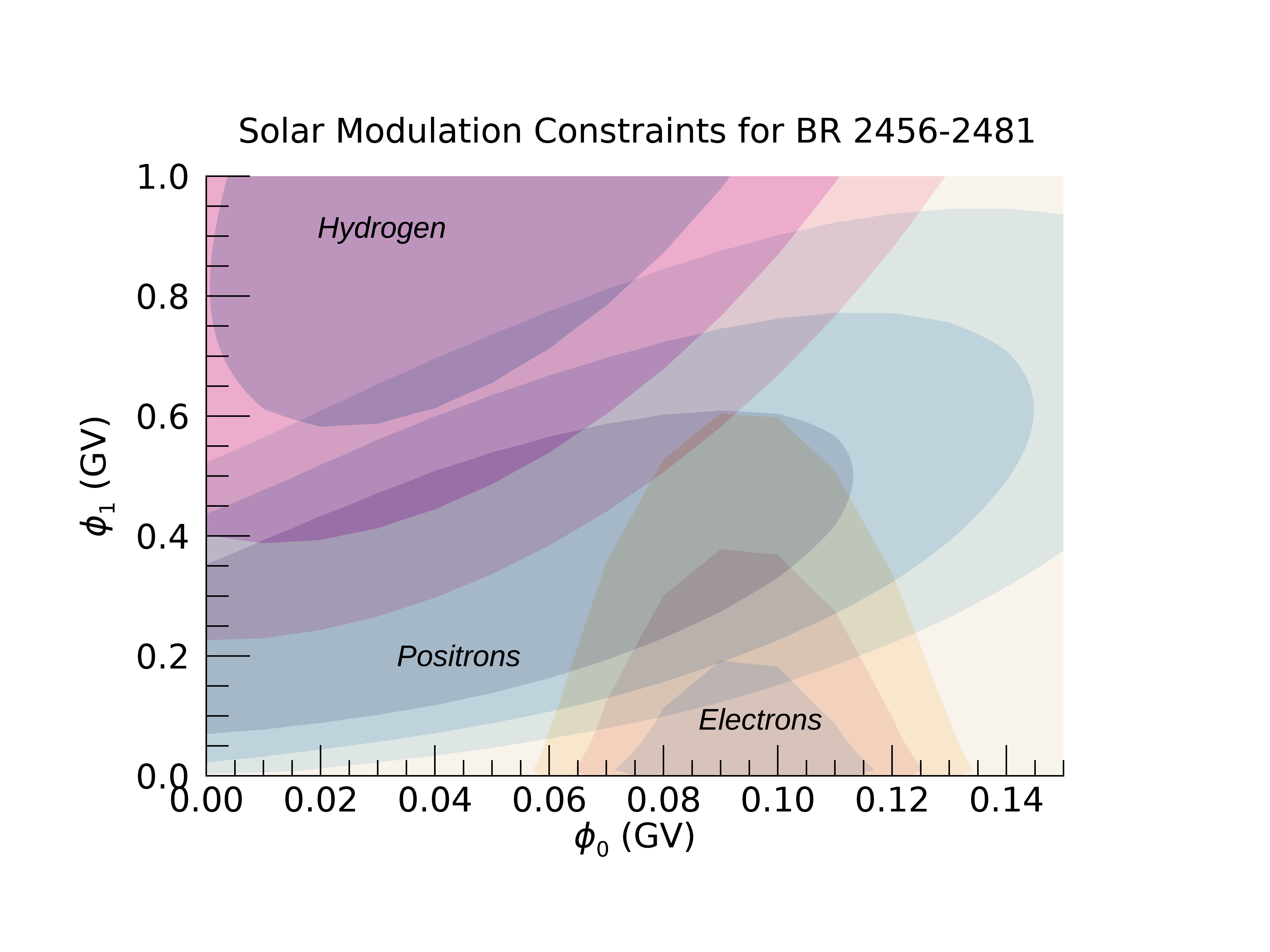
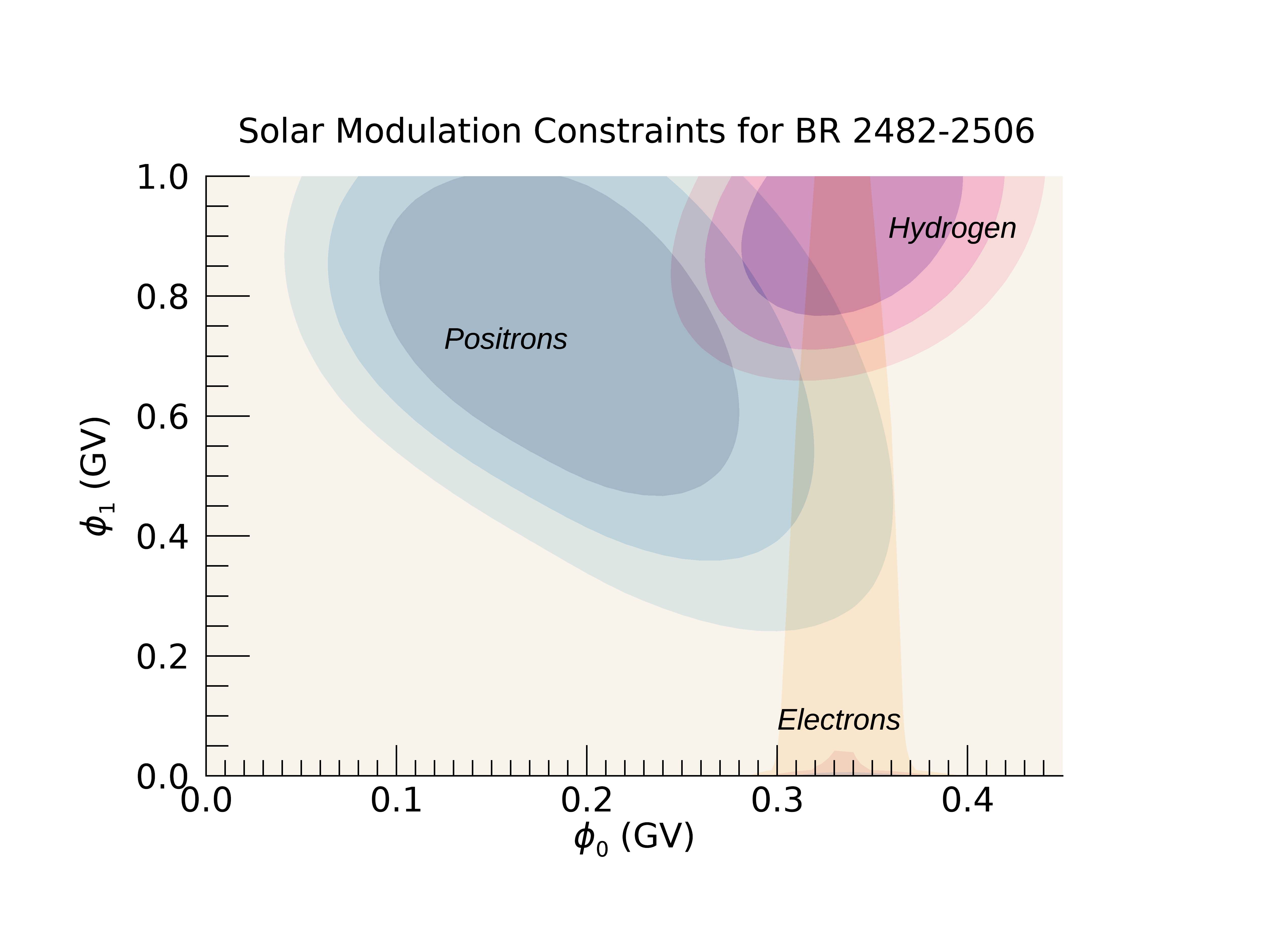
Figure 7: The, 1-, 2- and 3-$\sigma$ best fit projected ranges for $\phi_{0}$ and $\phi_{1}$ parameters. Left: the allowed ranges from the era or Bartels’ rotations 2456-2481 for hydrogen (purple), positrons (blue) and electrons (orange). Right: same as left but for the era or Bartels’ rotations 2482-2506. There is a significant shift in the $\phi_{0}$, $\phi_{1}$ parameter space between the two eras, that we associate to the fact that the heliospheric polarity that the cosmic rays experienced in the first of the two eras was not well defined (see text for further details).

We believe that the era of BR 2456-2481 represents an example of what happens to cosmic rays that propagate inwards closely after a Heliospheric polarity flip. On one hand their travel time is increased. That point we have tested by comparing the required averaging schemes for $B_{\rm tot}(t)$ and $\alpha(t)$ used in Eq. 2 to describe the charge-, time- and rigidity-dependence of solar modulation. We present the original publicly available ACE and WSO data in Fig. 1 and the averaged ones in Fig. 3. At the same time the actual energy losses the cosmic-rays experience are smaller than during times of established polarity as was the BR 2482-2506 era or the solar cycle 23 AMS-02 observations. This suggest that cosmic-rays during the era of non-well established polarity of within the volume of the Heliosphere (not just the surface of the Sun) travel through parts of it with weak magnetic fields.

We also point out that while the presence of the solar wind’s non-zero bulk speed is crucial in explaining the presence of drift effects along the HCS, its time-evolution is quite minimal and does not explain the observed time-variations of the measured cosmic-ray fluxes. This statement is true at least to first order level. Instead, our model does successfully associate the measured time evolution of $B_{\rm tot}(t)$ and $\alpha(t)$ to the observed cosmic-ray fluxes time-evolutions given in Figs. 2,  4, for the era of BR 2456-2481 and Figs. 5 and 6 for the BR 2482-2506.

The assumptions we make in this paper while still rely on the basic assumption that solar modulation of cosmic-ray fluxes can be described though a shift in the averaged kinetic energy of cosmic rays given by the modulation potential $\Phi$, that modulation potential’s value can be associated to the observable properties of the Heliosphere, which in our model following Ref. Cholis et al. (2016), are the measured amplitude of the magnetic field $B_{\rm tot}(t)$ at 1AU and HCS title angle $\alpha(t)$. Our $\phi_{1}$ term in Eq. 2, separates particles of opposite charge to account for the fact that depending on the polarity of the Heliospheric magnetic field cosmic rays travel on average through different volumes of the Heliosphere. Moreover, that term accounts for the presence of drift effects from the solar wind on the incoming cosmic rays that propagate through the HCS. Thus, our model explicitly breaks away from the conventional 1-D approach of the force field approximation Gleeson and Axford (1968) and while analytic it follows more closely to the lessons learned from more recent 3-D simulation work done by several authors as in Kota and Jokipii (1983); Caballero-Lopez and Moraal (2004); Potgieter (2013, 2017); Caballero-Lopez and Moraal (2004); Strauss et al. (2012); Qin and Shen (2017); Boschini et al. (2018); Jerome Boschini et al. (2019); Caballero-Lopez et al. (2019); Bisschoff et al. (2019). Furthermore, we have used the time-rich cosmic-ray and heliospheric magnetic field observations, to make a connection between the conditions in the Heliosphere and its effect on the measured cosmic-ray spectra. Our work does not aim to replace the achievements performed on the numerical side but provides a simple formula to account for solar modulation that through the continuous observations becomes better constrained. That in turn allows us to include in a computationally efficient way the effects of solar modulation when studying other types of astroparticle questions as the sources and environmental conditions of cosmic rays, their propagation through the ISM and in turn the ISM conditions. Another benefit of implementing a better constrained analytic prescription for the solar modulation, is the search for exotic sources of cosmic-rays as dark matter; that could contribute to the antimatter particle fluxes.

As future improvements, we need to account for the fact that the observed cosmic-ray fluxes are the result of particles having reached our detectors in a stochastic manner. Thus, while we assume averaged properties for the $B_{\rm tot}(t)$ and $\alpha(t)$ time-dependent quantities that we use to model the averaged energy losses expected in solar modulation, we need to account for the fact that cosmic-ray particles of a given species will have a scatter in these energy losses. We believe that may explain -especially for the case of the cosmic-ray electrons- some of the observed tensions between our model’s expectations and the observations. Another major improvement to be pursued for future work, is to understand better how the solar wind and its embedded magnetic field change with time at different radii. Here we rely on the timed measurements on a single radial position (at 1 AU). A model that can include the time evolution of the solar wind at different radii can be of great benefit in that goal. An example of work in that direction has been recently pursed in Li et al. (2022). Furthermore, in addition to the continuous observations by AMS-02, ACE and WSO, measurements from the Parker Solar Probe Fox et al. (2016) and the Solar Orbiter Müller et al. (2020) are going to provide useful future insights on the properties of the inner Heliosphere.

Acknowledgements: We would like to thank Tim Linden and Dan Hooper for collaboration on related work and in early stages of this project. We also acknowledge the use of GALPROP http://galprop.stanford.edu ; Strong and Moskalenko (1998); of GALPROP availabe at: https://galprop.stanford.edu/code.php . IC acknowledges support from the Michigan Space Grant Consortium, NASA Grants No. NNX15AJ20H and No. 80NSSC20M0124. IC acknowledges that this material is based upon work supported by the U.S. Department of Energy, Office of Science, Office of High Energy Physics, under Award No. DE-SC0022352.

References

- Usoskin et al. (2011) Ilya G. Usoskin, Galina A. Bazilevskaya, and Gennady A. Kovaltsov, “Solar modulation parameter for cosmic rays since 1936 reconstructed from ground-based neutron monitors and ionization chambers,” Journal of Geophysical Research (Space Physics) 116, A02104 (2011).
- Caballero-Lopez and Moraal (2012) Rogelio A. Caballero-Lopez and Harm Moraal, “Cosmic-ray yield and response functions in the atmosphere,” Journal of Geophysical Research (Space Physics) 117, 12103– (2012).
- Corti et al. (2019) Claudio Corti, Marius S. Potgieter, Veronica Bindi, Cristina Consolandi, Chris Light, Matteo Palermo, and Alexis Popkow, “Numerical modeling of galactic cosmic ray proton and helium observed by AMS-02 during the solar maximum of Solar Cycle 24,” Astrophys. J. 871, 253 (2019), arXiv:1810.09640 [astro-ph.SR] .
- Corti et al. (2020) Claudio Corti, Veronica Bindi, Cristina Consolandi, Christopher Freeman, Andrew Kuhlman, Christopher Light, Matteo Palermo, and Siqi Wang, “Test of validity of the force-field approximation with AMS-02 and PAMELA monthly fluxes,” PoS ICRC2019, 1070 (2020), arXiv:1910.00027 [astro-ph.HE] .
- Burger et al. (2022) R. A. Burger, A. E. Nel, and N. E. Engelbrecht, “Spectral properties of the n component of the heliospheric magnetic field from IMP and ACE observations for 1973– 2020,” The Astrophysical Journal 926, 128 (2022).
- Aguilar et al. (2013) M. Aguilar et al. (AMS), “First Result from the Alpha Magnetic Spectrometer on the International Space Station: Precision Measurement of the Positron Fraction in Primary Cosmic Rays of 0.5–350 GeV,” Phys. Rev. Lett. 110, 141102 (2013).
- Adriani et al. (2016) O. Adriani et al., “Time Dependence of the Electron and Positron Components of the Cosmic Radiation Measured by the PAMELA Experiment between July 2006 and December 2015,” Phys. Rev. Lett. 116, 241105 (2016), arXiv:1606.08626 [astro-ph.HE] .
- Abe et al. (2017) K. Abe et al., “The results from BESS-Polar experiment,” Adv. Space Res. 60, 806–814 (2017).
- Kachelriess et al. (2011) M. Kachelriess, S. Ostapchenko, and R. Tomas, “Antimatter production in supernova remnants,” Astrophys. J. 733, 119 (2011), arXiv:1103.5765 [astro-ph.HE] .
- Cholis and Hooper (2014) Ilias Cholis and Dan Hooper, “Constraining the origin of the rising cosmic ray positron fraction with the boron-to-carbon ratio,” Phys. Rev. D89, 043013 (2014), arXiv:1312.2952 [astro-ph.HE] .
- Hooper et al. (2015) Dan Hooper, Tim Linden, and Philipp Mertsch, “What Does The PAMELA Antiproton Spectrum Tell Us About Dark Matter?” JCAP 1503, 021 (2015), arXiv:1410.1527 [astro-ph.HE] .
- Mertsch and Sarkar (2014) Philipp Mertsch and Subir Sarkar, “AMS-02 data confront acceleration of cosmic ray secondaries in nearby sources,” Phys. Rev. D90, 061301 (2014), arXiv:1402.0855 [astro-ph.HE] .
- Strong (2015) A. W. Strong, “Recent extensions to GALPROP,” (2015), arXiv:1507.05020 [astro-ph.HE] .
- Kohri et al. (2016) Kazunori Kohri, Kunihito Ioka, Yutaka Fujita, and Ryo Yamazaki, “Can we explain AMS-02 antiproton and positron excesses simultaneously by nearby supernovae without pulsars or dark matter?” PTEP 2016, 021E01 (2016), arXiv:1505.01236 [astro-ph.HE] .
- Malkov et al. (2016) M. A. Malkov, P. H. Diamond, and R. Z. Sagdeev, “Positive charge prevalence in cosmic rays: Room for dark matter in the positron spectrum,” Phys. Rev. D94, 063006 (2016), arXiv:1607.01820 [astro-ph.HE] .
- Cuoco et al. (2017) Alessandro Cuoco, Michael Krämer, and Michael Korsmeier, “Novel Dark Matter Constraints from Antiprotons in Light of AMS-02,” Phys. Rev. Lett. 118, 191102 (2017), arXiv:1610.03071 [astro-ph.HE] .
- Cui et al. (2017) Ming-Yang Cui, Qiang Yuan, Yue-Lin Sming Tsai, and Yi-Zhong Fan, “Possible dark matter annihilation signal in the AMS-02 antiproton data,” Phys. Rev. Lett. 118, 191101 (2017), arXiv:1610.03840 [astro-ph.HE] .
- Cholis et al. (2017) Ilias Cholis, Dan Hooper, and Tim Linden, “Possible Evidence for the Stochastic Acceleration of Secondary Antiprotons by Supernova Remnants,” Phys. Rev. D95, 123007 (2017), arXiv:1701.04406 [astro-ph.HE] .
- Cholis et al. (2018) Ilias Cholis, Tanvi Karwal, and Marc Kamionkowski, “Studying the Milky Way pulsar population with cosmic-ray leptons,” Phys. Rev. D 98, 063008 (2018), arXiv:1807.05230 [astro-ph.HE] .
- Lowell et al. (2019) Alexander Lowell, Tsuguo Aramaki, and Ralph Bird (GAPS), “An Indirect Dark Matter Search Using Cosmic-Ray Antiparticles with GAPS,” PoS ICHEP2018, 543 (2019), arXiv:1812.04800 [physics.ins-det] .
- Kuhlen and Mertsch (2019) Marco Kuhlen and Philipp Mertsch, “Time-dependent AMS-02 electron-positron fluxes in an extended force-field model,” Phys. Rev. Lett. 123, 251104 (2019), arXiv:1909.01154 [astro-ph.HE] .
- Engelbrecht and Di Felice (2020) N. Eugene Engelbrecht and Valeria Di Felice, “Uncertainties implicit to the use of the force-field solutions to the parker transport equation in analyses of observed cosmic ray antiproton intensities,” Phys. Rev. D 102, 103007 (2020).
- Wang et al. (2019) Bing-Bing Wang, Xiao-Jun Bi, Kung Fang, Su-Jie Lin, and Peng-Fei Yin, “Time dependent solar modulation of cosmic rays from solar minimum to solar maximum,” Phys. Rev. D 100, 063006 (2019), arXiv:1904.03747 [astro-ph.HE] .
- Cholis et al. (2019) Ilias Cholis, Tim Linden, and Dan Hooper, “A Robust Excess in the Cosmic-Ray Antiproton Spectrum: Implications for Annihilating Dark Matter,” Phys. Rev. D99, 103026 (2019), arXiv:1903.02549 [astro-ph.HE] .
- Cuoco et al. (2019) Alessandro Cuoco, Jan Heisig, Lukas Klamt, Michael Korsmeier, and Michael Krämer, “Scrutinizing the evidence for dark matter in cosmic-ray antiprotons,” Phys. Rev. D 99, 103014 (2019), arXiv:1903.01472 [astro-ph.HE] .
- Heisig et al. (2020) Jan Heisig, Michael Korsmeier, and Martin Wolfgang Winkler, “Dark matter or correlated errors? Systematics of the AMS-02 antiproton excess,” (2020), arXiv:2005.04237 [astro-ph.HE] .
- Engelbrecht and Moloto (2021) N. Eugene Engelbrecht and K. D. Moloto, “An ab initio approach to antiproton modulation in the inner heliosphere,” The Astrophysical Journal 908, 167 (2021).
- Potgieter et al. (2021) M.S. Potgieter, O.P.M. Aslam, D. Bisschoff, and D. A Ngobeni, “Perspective on the Solar Modulation of Cosmic Anti-Matter,” Physics 3, 1190–1225 (2021).
- Cholis and Krommydas (2022) Ilias Cholis and Iason Krommydas, “Utilizing cosmic-ray positron and electron observations to probe the averaged properties of Milky Way pulsars,” Phys. Rev. D 105, 023015 (2022), arXiv:2111.05864 [astro-ph.HE] .
- Cholis et al. (2016) Ilias Cholis, Dan Hooper, and Tim Linden, “A Predictive Analytic Model for the Solar Modulation of Cosmic Rays,” Phys. Rev. D93, 043016 (2016), arXiv:1511.01507 [astro-ph.SR] .
- Gieseler et al. (2017) Jan Gieseler, Bernd Heber, and Konstantin Herbst, “An empirical modification of the force field approach to describe the modulation of galactic cosmic rays close to Earth in a broad range of rigidities,” J. Geophys. Res. Space Phys. 122, 10,964–10,979 (2017), arXiv:1710.10834 [physics.space-ph] .
- Aslam et al. (2019) O.P.M. Aslam, D. Bisschoff, M.S. Potgieter, M. Boezio, and R. Munini, “Modeling of Heliospheric Modulation of Cosmic-ray Positrons in a Very Quiet Heliosphere,” Astrophys. J. 873, 70 (2019), arXiv:1811.10710 [physics.space-ph] .
- Vittino et al. (2019) Andrea Vittino, Philipp Mertsch, Henning Gast, and Stefan Schael, “Breaks in interstellar spectra of positrons and electrons derived from time-dependent AMS data,” Phys. Rev. D 100, 043007 (2019), arXiv:1904.05899 [astro-ph.HE] .
- Smith et al. (1998) C. W. Smith, J. L’Heureux, N. F. Ness, M. H. Acuña, L. F. Burlaga, and J. Scheifele, “The ACE Magnetic Fields Experiment,” Space Science Rev. 86, 613–632 (1998).
- (35) http://www.srl.caltech.edu/ACE/ASC/, .
- (36) https://izw1.caltech.edu/ACE/ASC/level2/swepam_l2 desc.html, .
- (37) http://wso.stanford.edu/Tilts.html, .
- Heber and Potgieter (2006) B. Heber and M. S. Potgieter, “Cosmic Rays at High Heliolatitudes,” Space Science Rev. 127, 117–194 (2006).
- Jokipii and Thomas (1981) J. R. Jokipii and B. Thomas, “Effects of drift on the transport of cosmic rays. IV - Modulation by a wavy interplanetary current sheet,” Astrophys. J. 243, 1115–1122 (1981).
- Kota and Jokipii (1983) J. Kota and J. R. Jokipii, “Effects of drift on the transport of cosmic rays. VI - A three-dimensional model including diffusion,” Astrophys. J. 265, 573–581 (1983).
- Caballero-Lopez and Moraal (2004) R. A. Caballero-Lopez and H. Moraal, “Limitations of the force field equation to describe cosmic ray modulation,” Journal of Geophysical Research (Space Physics) 109, A01101 (2004).
- Potgieter (2013) Marius Potgieter, “Solar Modulation of Cosmic Rays,” Living Rev. Solar Phys. 10, 3 (2013), arXiv:1306.4421 [physics.space-ph] .
- Potgieter (2014) M.S. Potgieter, “The charge-sign dependent effect in the solar modulation of cosmic rays,” Advances in Space Research 53, 1415–1425 (2014), cosmic Ray Origins: Viktor Hess Centennial Anniversary.
- Potgieter (2017) M.S. Potgieter, “The global modulation of cosmic rays during a quiet heliosphere: A modeling perspective,” Advances in Space Research 60, 848–864 (2017), solar Energetic Particles, Solar Modulation and Space Radiation: New Opportunities in the AMS-02 Era.
- Gleeson and Axford (1968) L. J. Gleeson and W. I. Axford, “Solar Modulation of Galactic Cosmic Rays,” Astrophys. J. 154, 1011 (1968).
- Strauss et al. (2012) R. D. Strauss, M. S. Potgieter, I. Büsching, and A. Kopp, “Modelling heliospheric current sheet drift in stochastic cosmic ray transport models,” Astro. and Space Sci. 339, 223–236 (2012).
- Qin and Shen (2017) Gang Qin and Zhenning Shen, “Modulation of galactic cosmic rays in the inner heliosphere, comparing with pamela measurements,” The Astrophysical Journal 846, 56 (2017).
- Boschini et al. (2018) M. J. Boschini, S. Della Torre, M. Gervasi, D. Grandi, G. Jóhannesson, G. La Vacca, N. Masi, I. V. Moskalenko, S. Pensotti, T. A. Porter, L. Quadrani, P. G. Rancoita, D. Rozza, and M. Tacconi, “Deciphering the Local Interstellar Spectra of Primary Cosmic-Ray Species with HELMOD,” Astrophys. J. 858, 61 (2018), arXiv:1804.06956 [astro-ph.HE] .
- Jerome Boschini et al. (2019) Matteo Jerome Boschini, Stefano Della Torre, Massimo Gervasi, Giuseppe La Vacca, and Pier Giorgio Rancoita, “The HelMod Model in the Works for Inner and Outer Heliosphere: from AMS to Voyager Probes Observations,” arXiv e-prints , arXiv:1903.07501 (2019), arXiv:1903.07501 [physics.space-ph] .
- Caballero-Lopez et al. (2019) R. A. Caballero-Lopez, N. E. Engelbrecht, and J. D. Richardson, “Correlation of long-term cosmic-ray modulation with solar activity parameters,” The Astrophysical Journal 883, 73 (2019).
- Bisschoff et al. (2019) D. Bisschoff, M. S. Potgieter, and O. P. M. Aslam, “New Very Local Interstellar Spectra for Electrons, Positrons, Protons, and Light Cosmic Ray Nuclei,” Astrophys. J. 878, 59 (2019), arXiv:1902.10438 [astro-ph.HE] .
- Ferreira and Potgieter (2003) S.E.S. Ferreira and M.S. Potgieter, “Modulation over a 22-year cosmic ray cycle: On the tilt angles of the heliospheric current sheet,” Advances in Space Research 32, 657–662 (2003), heliosphere at Solar Maximum.
- Hoeksema (1992) J. T. Hoeksema, “Large-scale structure of the heliospheric magnetic field - 1976-1991,” in Solar Wind Seven Colloquium, edited by E. Marsch and R. Schwenn (1992) pp. 191–196.
- Ferreira and Potgieter (2004) S. E. S. Ferreira and M. S. Potgieter, “Long-Term Cosmic-Ray Modulation in the Heliosphere,” Astrophys. J. 603, 744–752 (2004).
- Cholis et al. (2020) Ilias Cholis, Dan Hooper, and Tim Linden, “Constraining the Charge-Sign and Rigidity-Dependence of Solar Modulation,” (2020), arXiv:2007.00669 [astro-ph.HE] .
- Aguilar et al. (2018a) M. Aguilar, L. Ali Cavasonza, B. Alpat, G. Ambrosi, L. Arruda, et al., and AMS Collaboration, “Observation of Fine Time Structures in the Cosmic Proton and Helium Fluxes with the Alpha Magnetic Spectrometer on the International Space Station,” Phys. Rev. Lett. 121, 051101 (2018a).
- Aguilar et al. (2018b) M. Aguilar, L. Ali Cavasonza, G. Ambrosi, L. Arruda, N. Attig, et al., and AMS Collaboration, “Observation of Complex Time Structures in the Cosmic-Ray Electron and Positron Fluxes with the Alpha Magnetic Spectrometer on the International Space Station,” Phys. Rev. Lett. 121, 051102 (2018b).
- Profumo (2011) Stefano Profumo, “Dissecting cosmic-ray electron-positron data with Occam’s Razor: the role of known Pulsars,” Central Eur. J. Phys. 10, 1–31 (2011), arXiv:0812.4457 [astro-ph] .
- Mertsch (2018) Philipp Mertsch, “Stochastic cosmic ray sources and the TeV break in the all-electron spectrum,” JCAP 11, 045 (2018), arXiv:1809.05104 [astro-ph.HE] .
- Cholis et al. (2022) Ilias Cholis, Yi-Ming Zhong, Samuel D. McDermott, and Joseph P. Surdutovich, “Return of the templates: Revisiting the Galactic Center excess with multimessenger observations,” Phys. Rev. D 105, 103023 (2022), arXiv:2112.09706 [astro-ph.HE] .
- Strong and Moskalenko (1998) A. W. Strong and I. V. Moskalenko, “Propagation of cosmic-ray nucleons in the Galaxy,” Astrophys. J. 509, 212–228 (1998), astro-ph/9807150 .
- (62) http://galprop.stanford.edu, .
- (63) Version 56 of GALPROP availabe at: https://galprop.stanford.edu/code.php, .
- Aguilar et al. (2019a) M. Aguilar et al. (AMS), “Towards Understanding the Origin of Cosmic-Ray Positrons,” Phys. Rev. Lett. 122, 041102 (2019a).
- Aguilar et al. (2019b) M. Aguilar et al. (AMS), “Towards Understanding the Origin of Cosmic-Ray Electrons,” Phys. Rev. Lett. 122, 101101 (2019b).
- Aguilar et al. (2021) M. Aguilar et al. (AMS), “The Alpha Magnetic Spectrometer (AMS) on the international space station: Part II — Results from the first seven years,” Phys. Rept. 894, 1–116 (2021).
- Ambrosi et al. (2017) G. Ambrosi et al. (DAMPE), “Direct detection of a break in the teraelectronvolt cosmic-ray spectrum of electrons and positrons,” Nature 552, 63–66 (2017), arXiv:1711.10981 [astro-ph.HE] .
- Adriani et al. (2018) O. Adriani et al., “Extended Measurement of the Cosmic-Ray Electron and Positron Spectrum from 11 GeV to 4.8 TeV with the Calorimetric Electron Telescope on the International Space Station,” Phys. Rev. Lett. 120, 261102 (2018), arXiv:1806.09728 [astro-ph.HE] .
- (69) http://wso.stanford.edu/Polar.html, .
- Li et al. (2022) Jung-Tsung Li, John F. Beacom, and Annika H. G. Peter, “Galactic Cosmic-Ray Propagation in the Inner Heliosphere: Improved Force-Field Model,” (2022), arXiv:2206.14815 [astro-ph.SR] .
- Fox et al. (2016) N. J. Fox, M. C. Velli, S. D. Bale, R. Decker, A. Driesman, R. A. Howard, J. C. Kasper, J. Kinnison, M. Kusterer, D. Lario, M. K. Lockwood, D. J. McComas, N. E. Raouafi, and A. Szabo, “The Solar Probe Plus Mission: Humanity’s First Visit to Our Star,” Space Science Rev. 204, 7–48 (2016).
- Müller et al. (2020) D. Müller, O. C. St. Cyr, I. Zouganelis, H. R. Gilbert, R. Marsden, T. Nieves-Chinchilla, E. Antonucci, F. Auchère, D. Berghmans, T. S. Horbury, R. A. Howard, S. Krucker, M. Maksimovic, C. J. Owen, P. Rochus, J. Rodriguez-Pacheco, M. Romoli, S. K. Solanki, R. Bruno, M. Carlsson, A. Fludra, L. Harra, D. M. Hassler, S. Livi, P. Louarn, H. Peter, U. Schühle, L. Teriaca, J. C. del Toro Iniesta, R. F. Wimmer-Schweingruber, E. Marsch, M. Velli, A. De Groof, A. Walsh, and D. Williams, “The Solar Orbiter mission. Science overview,” Astron. Astrophys. 642, A1 (2020), arXiv:2009.00861 [astro-ph.SR] .