Investigating field-induced magnetic order in Han Purple by neutron scattering up to 25.9 T

Abstract

BaCuSi₂O₆ is a quasi-two-dimensional (2D) quantum antiferromagnet containing three different types of stacked, square-lattice bilayer hosting spin-1/2 dimers. Although this compound has been studied extensively over the last two decades, the critical applied magnetic field required to close the dimer spin gap and induce magnetic order, which exceeds 23 T, has to date precluded any kind of neutron scattering investigation. However, the HFM/EXED instrument at the Helmholtz-Zentrum Berlin made this possible at magnetic fields up to 25.9 T. Thus we have used HFM/EXED to investigate the field-induced ordered phase, in particular to look for quasi-2D physics arising from the layered structure and from the different bilayer types. From neutron diffraction data, we determined the global dependence of the magnetic order parameter on both magnetic field and temperature, finding a form consistent with 3D quantum critical scaling; from this we deduce that the quasi-2D interactions and nonuniform layering of BaCuSi₂O₆ are not anisotropic enough to induce hallmarks of 2D physics. From neutron spectroscopy data, we measured the dispersion of the strongly Zeeman-split magnetic excitations, finding good agreement with the zero-field interaction parameters of BaCuSi₂O₆. We conclude that HFM/EXED allowed a significant extension in the application of neutron scattering techniques to the field range above 20 T and in particular opened new horizons in the study of field-induced magnetic quantum phase transitions.

I Introduction

One of the basic concepts of statistical physics is that any continuous classical or quantum phase transition (QPT) can be assigned to a certain universality class [Zinn-Justin2002]. Because the characteristic energy scale of a system vanishes and the correlation length diverges at such a transition, the microscopic details become irrelevant and the critical properties of the system are dictated only by global and scale-invariant characteristics such as the dimensionality, symmetry, and in special cases also the topology. Reducing the effective dimensionality of a system enhances the role of quantum fluctuations, leading to the emergence of exotic “low-dimensional” behavior.

Quantum magnetic systems are ideal testbeds for the study of phase transitions, criticality, and low-dimensional physics. One family of quantum magnets well suited for this task is spin-dimer systems, which consist of interacting spin-1/2 pairs with internal antiferromagnetic (AF) coupling, resulting in a global singlet ground state whose excitations are “triplons,” propagating triplet quasiparticles. When a sufficiently strong magnetic field is applied, a QPT takes place from the dimer-singlet phase, which magnetically is quantum disordered to a field-induced ordered phase resembling an effective XY spin model [Sachdev2011]. The magnetization of the dimers in this ordered phase can be separated into a longitudinal component, $m_{\parallel}$, along the field direction and a transverse component, $m_{\perp}$, perpendicular to the field; $m_{\parallel}$ is of necessity ferromagnetic (FM) and local in nature, whereas $m_{\perp}$ is AF as a result of the interactions both within and between the dimers [Matsumoto2004], and its magnitude represents the order parameter.

If the interaction network has dimensionality $d=3$, the phase transition is in the 3D-XY universality class [Giamarchi2008; Zapf2014] and the field-induced ground state has the critical behavior of a Bose-Einstein Condensate (BEC) [Bose1924; Einstein1924], as observed experimentally for example in the 3D spin-dimer material TlCuCl₃ [Nikuni2000; Tanaka2001; Oosawa2001; Rueegg2003; Glazkov2004]. In systems with $d\leq$ 2, the field-induced phase cannot possess long-range order (LRO) at finite temperatures due to the Mermin-Wagner theorem [Mermin1966], but quasi-ordered phases may nevertheless be found in systems with weak interactions between low-dimensional substructures (e.g. chains, ladders, or planes) when the temperature exceeds the weak energy scale. Spin-dimer systems with $d=1$ exhibit a field-induced phase that resembles a Tomonaga-Luttinger liquid (TLL), with algebraically decaying spin-spin correlations in the ground state and fractional (spin-1/2) excitations in the spectrum [Sachdev1994; Giamarchi1999; Giamarchi2003]. For spin-dimer systems with $d=2$, the field-induced phase is equivalent to the 2D-XY model, which is special because of the Berezinskii-Kosterlitz-Thouless (BKT) transition [Berezinskii1971; Kosterlitz1973] from a quasi-ordered phase with algebraically decaying spin correlations at lower temperatures to a disordered phase with exponentially decaying correlations. Quasi-low-dimensional spin-dimer materials consist of low-dimensional substructures such as chains, ladders, or (bi)layers that are strongly coupled internally but weakly coupled to each other. Such systems display 3D coherence up to a certain temperature, above which thermal fluctuations destroy 3D LRO to produce different forms of low-dimensional behavior.

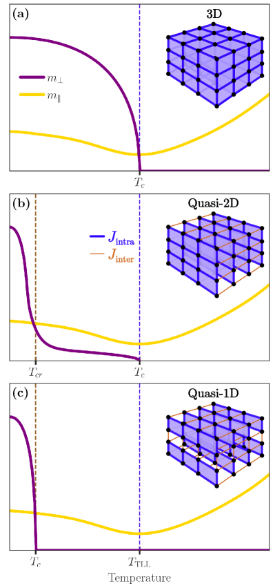
Figure 1: Schematic temperature-dependence of the longitudinal magnetization, $m_{\parallel}$, and the transverse magnetization, $m_{\perp}$, in the field-induced ordered phases of spin-dimer systems whose substructures, with characteristic energy scale $J_{\rm intra}$, have different dimensionalities and weak mutual coupling $J_{\rm inter}$. (a) 3D. (b) 2D, showing an example in which $m_{\perp}$ undergoes particularly strong thermal suppression at $T_{\rm cr}$, but nevertheless remains finite up to $T_{c}$ [Furuya2016]. (c) 1D, where $T_{c}$ is determined by $J_{\rm inter}$ whereas $J_{\rm intra}$ governs the behavior only of the substructure, setting the characteristic temperature $T_{\rm TLL}$.

To see how certain hallmarks of low-dimensional physics manifest themselves in the temperature-dependence of $m_{\perp}$ and $m_{\parallel}$ in the field-induced ordered phase, Fig. 1 represents both quantities as functions of temperature for spin-dimer systems with different substructure dimensionalities. In 3D, $m_{\parallel}$ displays a minimum where magnetic order is lost, before increasing as the rising temperature causes a preferential population of the lowest of the Zeeman-split triplet states [Fig. 1(a)], and this property was used to define the phase boundary in TlCuCl₃ [Nikuni2000]. This minimum marks the point where thermal fluctuations destroy coherence within the low-dimensional substructure, and hence it still corresponds to $T_{c}$ in a quasi-2D system [Fig. 1(b)]. By contrast, in a quasi-1D system [Fig. 1(c)] it indicates only a crossover temperature, $T_{\rm TLL}$, out of the quasi-ordered TLL phase [Maeda2007], and this physics has been observed in the two spin-ladder compounds BPCB [(C₅H₁₂N])₂CuBr₄] [Klanjsek2008; Lorenz2008; Thielemann2009] and DIMPY [(C₇H₁₀N)₂CuBr₄] [Schmidiger2012; Ninios2012]. Turning to the order parameter, in 3D and quasi-1D systems [Figs. 1(a) and 1(c)] $m_{\perp}$ shows a conventional temperature-dependence, but it has been proposed [Furuya2016] that a quite different form could be observed in sufficiently 2D systems [Fig. 1(b)]. In this scenario, $m_{\perp}$ falls rapidly at low temperatures as 3D coherence is lost, before attaining a steady but strongly suppressed value beyond a crossover temperature, $T_{\rm cr}$, and remaining finite up to a critical temperature, $T_{c}$; although the magnitude of $T_{c}$ is characteristic of the in-plane (2D) energy scale, the critical properties around it may be 3D nature.

While the forms of $m_{\parallel}$ and $m_{\perp}$ depicted in Fig. 1 have been confirmed by neutron diffraction and nuclear magnetic resonance (NMR) in 3D [Nikuni2000; Tanaka2001] and in quasi-1D spin-dimer materials [Thielemann2009; Ninios2012], the special quasi-2D form of $m_{\perp}$ has not so far been observed. This raises the question of which quasi-2D spin-dimer material may offer a suitable candidate to search for such hallmarks of 2D physics. As reviewed recently in Ref. [Allenspach2021], quasi-2D materials including the Shastry-Sutherland compound SrCu₂(BO₃)₂ [Kageyama1999], the “triplon-breakdown” compound (C₄H₁₂N₂)Cu₂Cl₆ (PHCC) [Stone2001; Stone2006], and the triangular-dimer-lattice chromate compounds Ba₃Cr₂O₈ [Nakajima2006; Kofu2009; Aczel2009a] and Sr₃Cr₂O₈ [Aczel2009b; Islam2010; Nomura2020] all have additional physics that appear to remove them from consideration in this context. Although a possible BKT phase has been reported in the metal-organic material TK91 [C₃₆H₄₈Cu₂F₆N₈O₁₂S₂], which consists of stacked and distorted honeycomb planes [Tutsch2014], the maximal temperature for quasi-LRO of 50 mK poses a serious challenge to a systematic experimental investigation by neutron diffraction or NMR.

BaCuSi₂O₆ is both a purple pigment known in ancient China [FitzHugh1992] and a quasi-2D quantum magnet composed of $S=1/2$ Cu²⁺ dimers arranged in a square-lattice geometry with offset bilayer stacking. Early experiments by torque magnetometry were interpreted as indicating a counterintuitive reduction of the effective system dimension from 3D to 2D as the temperature was reduced towards the field-induced critical point [Sebastian2006], which was presumed to be a consequence of frustrated inter-bilayer interactions. However, intensive subsequent investigation revealed that the low-temperature phase contains three different types of structurally [Samulon2006; Sheptyakov2012] and magnetically [Rueegg2007; Kraemer2007] inequivalent bilayer, and as we discuss in Sec. II this both explains the presence of an anomalous critical scaling regime, previously misinterpreted as dimensional reduction [Allenspach2020], and offers a qualitatively different route to realizing the quasi-2D physics of Fig. 1(b) [Furuya2016].

Although neutron scattering is the method of choice for characterizing the structure and excitations of magnetic states, its application to the field-induced ordered phase of BaCuSi₂O₆ has to date been impossible due the fact that the critical magnetic field is 23.35 T. Here we report a neutron scattering study of BaCuSi₂O₆ at fields up to 25.9 T, made possible by the HFM/EXED facility, which was installed and operated at the Helmholtz-Zentrum Berlin from 2015 until 2019. Working in diffraction mode, we measure the intensities of a number of Bragg peaks of the ordered phase as functions of magnetic field and temperature, and perform a thorough statistical analysis to identify the evolution of the magnetic order parameter. In spectroscopy mode, we measure the magnetic excitations at fields both below and within the regime of field-induced order, and compare these to the modes expected on the basis of the interactions determined at zero field.

The structure of this article is as follows. In Sec. II we summarize the collected body of knowledge concerning BaCuSi₂O₆ and introduce the possible consequences of its inequivalent layering. In Sec. III we introduce the instrument HFM/EXED and the experimental possibilities it allowed. Section IV presents the results of our diffraction measurements and a systematic global analysis of these data. In Sec. V we discuss the evolution of the magnetic excitation spectrum as a function of the applied field. Section VI contains a brief discussion and conclusion.

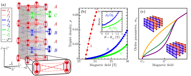
Figure 2: (a) Representation of a primitive unit cell of BaCuSi₂O₆. The three distinct bilayer types are labelled A, B, and C, and their ABABAC stacking sequence gives them population ratios 3:2:1. The minimal magnetic model requires the intra-dimer, inter-dimer, and inter-bilayer Heisenberg interactions $\{J_{\sigma},J_{\sigma}^{\prime},J^{\prime\prime}\}$; the effective inter-dimer interaction parameters within each bilayer ($J_{\sigma}^{\prime}$, edges of colored squares) are sums of four pairwise ionic interactions (inset). (b) Triplon occupations in the three types of bilayer, computed by quantum Monte Carlo for unrenormalized $\{J\}$ parameters and shown as a function of field at an effective temperature $T=100$ mK. Inset: occupation ratios. (Both panels from Ref. [Allenspach2021]). (c) Schematic representation of the field-induced magnetic order parameter, $m_{\perp}$, at zero temperature for a magnetic model of inequivalent stacked bilayers. For an approximately uniform model, meaning with near-equivalent layers (yellow), one expects a conventional growth of $m_{\perp}$ with a conventionally broad regime of 3D critical scaling. For an extremely non-uniform model, with $J_{B}-J_{A}\gg J^{\prime\prime}$ (violet), one expects $m_{\perp}$ to become finite once $H$ exceeds the gap of the A bilayers, but to remain strongly suppressed over the regime $H_{c1}<H<H^{*}$, where $H^{*}-H_{\rm c1}=(J_{B}-J_{A})/g\mu_{B}\mu_{0}$, until the field establishes a significant triplon occupation on all bilayers. For a model of intermediate uniformity (dark green), one may expect a partial suppression of $m_{\perp}$ above $H_{c1}$ that acts to reduce the regime of 3D critical scaling very strongly.

II BaCuSi₂O₆

The spin-dimer compound BaCuSi₂O₆ forms large, purple-colored single crystals. The Cu²⁺ ions provide $S=1/2$ quantum spins, which are coupled first into dimer units, which in turn form square-lattice bilayers, and finally these bilayers are stacked with a relative [1/2 1/2] offset to form the 3D structure. At room temperature there is only one type of bilayer [Sparta2006; Samulon2006], but BaCuSi₂O₆ undergoes a structural phase transition below 90 K to a weakly orthorhombic structure [Samulon2006], in which the adjacent bilayers become structurally inequivalent [Sheptyakov2012]. At zero field, the ground state is a global singlet, whose triplon excitations have a gap of 3.15 meV, and early neutron scattering [Rueegg2007] and NMR investigations [Kraemer2007; Kraemer2013] demonstrated from the presence of multiple triplon modes that the different bilayer types also become magnetically inequivalent.

While the critical field required to close the spin gap, $\mu_{0}H_{c1}=23.35$ T for ${\hat{H}}\parallel{\hat{c}}$, has excluded neutron scattering as a probe of the field-induced ordered phase, NMR and a number of other high-field experimental techniques [Jaime2004; Sebastian2005; Sebastian2006] have been applied to measure the field-temperature phase boundary. An effort to analyze the critical scaling of this phase boundary, as extracted from detailed torque magnetometry measurements [Sebastian2006], led the authors to propose an unusual dimensional reduction, from 3D to 2D scaling, on approaching the quantum critical point. The origin of this behavior was proposed to lie in the exact frustration of the presumed AF interactions between the offset bilayers, and was supported by some subsequent theoretical studies [Batista2007; Schmalian2008] but contested by others [Maltseva2005; Roesch2007a], notably those including the inequivalent bilayers [Roesch2007b].

The situation was resolved for BaCuSi₂O₆ by the theoretical observation [Mazurenko2014] that the inter-dimer interactions within each bilayer should in fact be effectively FM, as a consequence of the relative couplings between ion pairs represented in the inset of Fig. 2(a). This would mean that the inter-bilayer interactions are entirely unfrustrated, obviating the dimensional reduction scenario. Inelastic neutron scattering (INS) studies at zero magnetic field verified this situation experimentally [Allenspach2020] by confirming the presence of three triplon modes, previously observed in Ref. [Rueegg2007], establishing an ABABAC $c$-axis stacking of the three corresponding magnetic bilayer types (labelled in ascending order of triplon energy as A, B, and C), and determining that the spin Hamiltonian, depicted in Fig. 2(a), has effective FM intra-bilayer and unfrustrated AF inter-bilayer interactions. It is clear from Fig. 2(a) that the bilayer stacking introduces an energy scale $J_{B}-J_{A}$, and with it a regime of magnetic field directly above $H_{c1}$ where the response of the different bilayers to the applied field will not be the same, a result confirmed [Allenspach2020] by quantum Monte Carlo (QMC) simulations of the bilayer triplon densities [Fig. 2(b)]. For the 3D critical scaling of the ABABAC system, the important quantity is the energy scale ${\tilde{J}}^{\prime\prime}=(J^{\prime\prime})^{2}/[J_{B}-J_{A}]$, which is approximately 0.04 K in BaCuSi₂O₆ [Allenspach2020], because thermal fluctuations above this scale may cause an effective decoupling of the triplon-condensed $A$ bilayers. This converts the true 3D scaling into an anomalous effective scaling regime, which arises from the bilayer inequivalence and was originally misinterpreted as dimensional reduction.

The concept of non-uniform layering raises the prospect of a dramatic strengthening, encapsulated in the renormalization of $J^{\prime\prime}$ to ${\tilde{J}}^{\prime\prime}$, of the quasi-2D nature of a system, and hence of the possibility that the physics of Fig. 1(b) could be observed in experiment. Now that neutron scattering measurements have become possible at the low edge of the field-induced magnetically ordered phase in BaCuSi₂O₆, precisely where the different bilayers respond differently [Fig. 2(b)], one may anticipate how the order parameter could evolve for different degrees of non-uniformity in the bilayer properties. Figure 2(c) depicts the contrast between the conventional growth of $m_{\perp}$ with $H$ for a uniform system ($J_{B}-J_{A}<J^{\prime\prime}$), and a situation where the extremely non-uniform bilayer properties ($J_{B}-J_{A}\gg J^{\prime\prime}$) ensure a wide regime of applied field in which the triplon gap would be closed on an isolated A bilayer but not on a B bilayer. In this region, the B bilayer has only weak, proximity-induced magnetic order arising from the A-bilayer condensation and the interlayer coupling, and one may expect the order parameter to remain suppressed until the field is large enough to create a significant B-bilayer triplon condensation. As the bilayers are made more similar, first the suppression would become less pronounced and then one may not observe a non-monotonic first derivative in $m_{\perp}(H)$, but it is clear that any finite $J_{B}-J_{A}>J^{\prime\prime}$ will act to curtail the regime of true 3D critical scaling (as observed in Ref. [Allenspach2020]). We stress that the regime of suppressed $m_{\perp}(H)$ for the non-uniform bilayer stack in Fig. 2(c) has no direct correspondence with the finite-temperature plateau in $m_{\perp}(T)$ shown in Fig. 1(b); the latter is proposed [Furuya2016] to be a property even of a uniform stack (depicted in the figure inset), and its field response is that of the yellow curve in Fig. 2(c). The non-uniform stack should not only improve the prospects for observing such extreme 2D physics in $m_{\perp}(T)$ but also offer a less stringent possibility, in $m_{\perp}(H)$, for observing a response function reflecting 2D substructures behaving in a quasi-isolated manner.

Next we comment that reducing the non-uniformity of the bilayer stacking in BaCuSi₂O₆ has already been achieved. Stoichiometric substitution of Sr for Ba ions acts to suppress the 90 K structural phase transition, with 5% Sr being sufficient to stabilize the tetragonal structure down to the lowest temperatures [Puphal2016]. INS measurements of Ba_0.9Sr_0.1CuSi₂O₆ at zero magnetic field confirmed that there is only one type of bilayer at 1.5 K and determined the spin Hamiltonian [Allenspach2021]. NMR measurements were performed at high magnetic fields and low temperatures to determine the phase boundary of field-induced order, and a detailed analysis revealed 3D quantum critical scaling with no hallmarks of anomalous behavior. Similarly, the relative order parameter extracted from the NMR spectra showed no deviation from the conventional form [Allenspach2021]. Because the ratio of intra- to inter-bilayer interactions is 25 in Ba_0.9Sr_0.1CuSi₂O₆ (a value double that of the unsubstituted system [Allenspach2020]), it is clear that, for a uniform bilayer stack, this value of the interaction ratio is not sufficiently close to the quasi-2D regime to observe any of the fingerprints of 2D physics proposed in Fig. 1(b).

Based on this result we observe that, even if samples were found that realize interaction ratios orders of magnitude beyond the value of 25, the regime where the order parameter exhibits quantum critical scaling would be pushed below mK temperatures and would become impossible to investigate by present methods. By contrast, creating non-uniform layered structures falls within present technological capabilities for engineering atomically thin magnetic materials [Gibertini2019; Klein2019; Ubrig2019; Cao2019; Wang2019; Kim2019]. While still relying on the non-uniform layering occurring naturally in BaCuSi₂O₆, we will use our ability to perform direct measurements of the order parameter to investigate whether this degree of non-uniformity is sufficient to provide one of the unconventional curves shown in Fig. 2(c).

III HFM/EXED

The benchmark value for the critical field of BaCuSi₂O₆ is $\mu_{0}H_{c1}=23.35$ T, determined by ²⁹Si NMR measurements with the field aligned along the sample $c$ axis [Kraemer2007]. Thus the field-induced ordered phase has remained inaccessible to the conventional superconducting magnets used in neutron scattering experiments, which are limited to maximal static magnetic fields of 17 T. However, neutron scattering measurements were possible at higher fields on the Extreme Environment Diffractometer (EXED) within the High Field Magnet (HFM) facility [Prokhnenko2017] at the Helmholtz-Zentrum Berlin, which operated from 2015 to 2019.

HFM was a horizontal, series-connected hybrid magnet consisting of three concentric solenoids, an outer superconducting coil and a combination of two inner, normal conducting coils [Smeibidl2016]. Magnetic fields up to 26 T could be reached with a 4 MW inner coil at an operating current of 20 kA. These fields were maintained across the 50 mm diameter of the warm bore, in which the cryostat was installed, with a field homogeneity of 0.5% across a cryogenic sample volume of order (15 mm)³. EXED was a time-of-flight (TOF) neutron instrument built at HFM that had three different modes of operation, namely diffraction, spectroscopy, and low-$Q$ [Bartkowiak2015; Prokhnenko2015; Prokhnenko2017]. We refer henceforth to the combination of HFM and EXED as HFM/EXED.

The primary targets for a neutron scattering characterization of the field-induced ordered phase are the magnetic order parameter, $m_{\perp}$, and the dispersion of the magnetic excitations throughout the Brillouin zone. Concerning the order parameter, NMR is sensitive to the local magnetization of the Cu²⁺ ions through the positions of the peaks in the spectrum, and thus a relative $m_{\perp}$ can in principle be extracted as a function of field and temperature from the frequency splitting of these peaks [Berthier2017; Allenspach2021]. However, this turned out not to be possible in BaCuSi₂O₆ because of the broad and complex line shapes caused by the incommensurability present in the low-temperature structure [Samulon2006; Sheptyakov2012; Stern2014]. By contrast, neutron diffraction allows a direct determination of $m_{\perp}$, from the intensity of the magnetic Bragg peaks, whose location can be well separated from the nuclear Bragg peaks. In fact the magnetic Bragg peaks accessible in BaCuSi₂O₆ with the alignment we used on HFM/EXED do coincide with the locations of the nuclear Bragg peaks, a situation that is readily dealt with by including the nuclear contribution within the global intensity model used to fit the diffraction data (Sec. IVC). Regarding the dispersion relation of magnetic excitations, there is no alternative to inelastic neutron scattering.

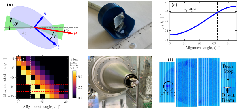
Figure 3: Summary of the experimental conditions on HFM/EXED. (a) Top view of the scattering plane, illustrating the magnet rotation angle, $\psi$, and sample alignment angle, $\zeta$. The $g$-factor [Zvyagin2006] is represented as the (exaggerated) blue ellipse and its values in the field of the experiment therefore depend on $\zeta$. The 30^∘ conical opening allowed by the magnet is indicated by the green area. (b) 3D-printed sample chamber and aluminum sample holder. (c) Critical field, $\mu_{0}H_{c1}$, shown as a function of $\zeta$. The horizontal line corresponds to the maximum magnetic field achievable on HFM/EXED (25.9 T) and imposes an upper limit for $\zeta$ (dashed vertical line). (d) Neutron flux on HFM/EXED modelled for the ($-2$ 0 2) Bragg peak of BaCuSi₂O₆; pixels with zero flux within the region of detector coverage are a consequence of neutrons scattered into gaps between detector elements. The dashed white line indicates the chosen $\zeta$ (22.5^∘) and the red dashed lines the chosen $\psi$ values ($-9.5^{\circ}$ and $-11^{\circ}$). (e) Sample installed below the cold finger of the cryostat. (f) Forward-scattering detector panels of HFM/EXED, displaying an example of the neutron intensity of BaCuSi₂O₆ collected in diffraction mode.

HFM/EXED offered a solution to both problems, in that the measurements of magnetic order presented in Sec. IV were performed in diffraction mode and the inelastic data discussed in Sec. V were collected in spectroscopy mode. Figure 3(a) shows the scattering geometry of the experiments. The magnetic field was applied horizontally and the magnet could be rotated by an angle, $\psi$, of up to 12^∘ relative to the beam of incoming neutrons, which had wave vectors $\vec{k}_{i}$. The sample was aligned with ($h$ 0 $l$) in the horizontal scattering plane and the angle between the magnetic field and the $c$ axis of the sample, $\zeta$, is referred to henceforth as the alignment angle. Because the alignment could not be changed once the sample was installed inside the cryostats used (Sec. IV.1), $\zeta$ had to be selected before the experiments. Incoming neutrons entering the sample chamber were scattered to the detector through cone-shaped openings, which subtended an angle of 30^∘ and are shown as the green areas in Fig. 3(a).

There were three factors to be taken into account for the choice of $\zeta$. (i) The sample had to be aligned to fit into the sample chamber of the cryostat. To ensure this, a 1:1 model of the sample chamber was produced by 3D printing, and is shown in Fig. 3(b) together with the sample holder. (ii) The critical field varies with the direction of the applied magnetic field, because $\mu_{0}H_{c1}=\Delta/(g\mu_{B})$, where $\Delta$ is the spin gap, and the effectively temperature-independent $g$-factor of BaCuSi₂O₆ has an anisotropy of approximately 12%, with $g_{cc}=2.306(3)$ and $g_{aa}=g_{bb}=2.050(3)$ [Zvyagin2006]. Thus we estimated that $\mu_{0}H_{c1}=23.57$ T when the field direction is parallel to the $c$ axis ($\zeta=0^{\circ}$) and 26.15 T when the field is within the $ab$ plane ($\zeta$ = 90^∘) [Fig. 3(c)] (the latter case making the field-induced phase inaccessible on HFM/EXED). The alignment angle therefore had to be made as small as possible to maximize access to the field-induced phase. (iii) It was necessary to choose magnetic Bragg peaks that are both strong, to obtain sufficient counting statistics, and maximize the ratio of the magnetic to the nuclear signal. Because the 30^∘ opening angle of the magnet restricted the $\vec{Q}$-range accessible on HFM/EXED, the choice of Bragg peak placed a further constraint on the possible value of $\zeta$.

Based on these three factors, we decided to align the sample with $\zeta=22.5^{\circ}$. This alignment allows access to the ($-2$ 0 2) Bragg peak, which we estimated by structure-factor calculations to have a sufficient ratio between its magnetic and nuclear intensities to optimize the extraction of the magnetic signal. The specific choice of 22.5^∘ was based on neutron flux calculations performed for the ($-2$ 0 2) Bragg peak with the beam-line software EXEQ [Bartkowiak2020], whose results are shown in Fig. 3(d). All of our experiments were performed with a single-crystal sample of BaCuSi₂O₆ of weight 1.01 g, which had already been used for the zero-field INS measurements reported in Ref. [Allenspach2020].

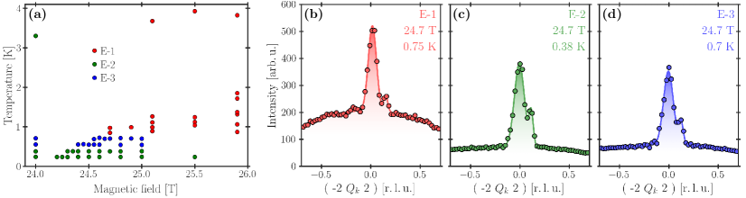
Figure 4: (a) Overview of the different points in the ($\mu_{0}H,T$) phase diagram at which the ($-2$ 0 2) Bragg peak was measured during the three experiments E-1, E-2, and E-3. (b-d) Intensity measured along ($-2$ $Q_{k}$ 2). Symbols show the normalized intensity obtained by integrating the data over $h$ and $l$. Solid lines display the results of individual fits using an intensity model of two Gaussians and a polynomial background, as described in the text.

IV Neutron Diffraction Measurements

IV.1 Experimental Conditions

Diffraction data were collected during three different experiments, which in the following we label E-1, E-2, and E-3. In E-1, a ³He cryostat was used to reach temperatures down to 0.6 K, while in E-2 and E-3 the sample was installed in a dilution cryostat with the same geometry, but which allowed us to extend the measurements down to 0.25 K. Figure 3(e) shows the sample mounted on the cold finger of the cryostat. The rotation of the magnet relative to the incoming neutron beam, $\psi$, was selected as $-9.5^{\circ}$ for E-1 and $-11^{\circ}$ for E-2 and E-3. These values were chosen not only to maximize the incoming neutron flux for the ($-2$ 0 2) Bragg peak but also to avoid having parts of this peak cut off by the edges of or gaps in the detector. The chopper settings were adjusted for each experiment so that the wavelength band of the incoming neutrons was centered on the ($\psi$-dependent) wavelength of the ($-2$ 0 2) peak and had a width of 1 Å. Although the sample was removed from the cryostats between the experiments, the alignment angle was set to the same initial value for all three experiments. Nevertheless, even with $\zeta$ aligned to 22.5^∘, the cold fingers of the two cryostats were not identical, causing a field- and temperature-dependent misalignment that affected both the in-plane and out-of-plane positions of the ($-2$ 0 2) Bragg peak. The out-of-plane misalignment is visible in Fig. 3(f) as a vertical offset of this peak on the forward-scattering detector panel. The additional bend in the cold finger when applying a magnetic field was found to be $\delta\zeta\leq 0.3^{\circ}$ between 0 and 25.9 T, and this further offset was the same for both cryostats and thus in all experiments.

The elastic signal of BaCuSi₂O₆ was measured for the combination of magnetic fields and temperatures, ($\mu_{0}H$, $T$), shown in Fig. 4(a). Data were collected by scanning either the temperature or the field, while keeping the other constant. These scans started either at the lowest temperature or the highest field value, where the magnetic order was strongest in the field-induced phase. Either the temperature was then increased or the magnetic field was decreased until the magnetic order had vanished. Afterwards the temperature was increased to 3.5 K before changing the field for the next scan, or the magnetic field was set to 24 T before changing the temperature. The goal of this procedure was to minimize potential hysteresis effects in our measured order parameter. Due to the limited amount of measurement time, we included only a small set of ($\mu_{0}H,T)$ points in the disordered phase, and chose these to cover a wide range of fields and temperatures. To obtain sufficient statistics for the magnetic signal on top of the nuclear signal, the data-acquisition time was adjusted for each ($\mu_{0}H,T$) point within the ordered phase based on its distance to the phase boundary, where $m_{\perp}\rightarrow 0$, and ranged from 3 to 16 hours.

A temperature sensor was attached to the cold fingers of the cryostats and measured a time series of temperature data for each ($\mu_{0}H,T$) point. The sample temperatures and their uncertainties at every point were estimated based on the mean and standard deviation of each time series. The magnetic field of HFM/EXED was calibrated in lower fields and extrapolated to the highest field values. From other experiments performed on HFM/EXED [Prokes2017; Fogh2020; Prokes2020], this extrapolation is known to result in highly accurate estimates of the field values and thus the uncertainties in the fields were assumed to be zero throughout the analysis to follow.

IV.2 Extraction of the Peak Intensities

The measured data were preprocessed and transformed into $\vec{Q}$-space using the software Mantid [Arnold2014]. During the preprocessing step, the neutron counts were integrated over the wavelength band of the scattered neutrons, normalized by the monitor and a vanadium standard, and rescaled by the Lorentz polarization factor [Debye1913] and by taking the sample misalignment into account. One-dimensional cuts were extracted from the preprocessed data along ($-2$ $Q_{k}$ 2) by integrating over [$-2.15$,$-1.85$] in $h$ and [1.85,2.15] in $l$ for each ($\mu_{0}H,T$) point, resulting in the normalized intensities $I(Q_{k},\mu_{0}H,T)$. In addition to the ($-2$ 0 2) peak, the ($-2$ $\pm 1$ 2) Bragg peaks are also included in these cuts, but have only a weak magnetic signal. These peaks were used to verify the absence of any magnetostriction effects, by which the nuclear intensity is modified due to field-induced changes of the crystal structure. Although magnetostriction does not affect all Bragg peaks equally, structural changes affecting the ($-2$ 0 2) peak would also be visible in the ($-2$ $\pm$1 2) peaks.

Figures 4(b)-(d) display the cuts along ($-2$ $Q_{k}$ 2) obtained in each of the three experimental runs, E-1, E-2, and E-3. In addition to the main peak centered at $Q_{k}=0$, a smaller side peak is visible at $Q_{k}\approx 0.15$. This second peak has the same field- and temperature-dependence as the main peak and appears in the same location in the forward- and backscattering detector panels, from which we deduce that it is most probably a consequence of divergence in the beam profile across the sample volume. While the background is almost flat and comparable in intensity for the cuts obtained in E-2 [Fig. 4(c)] and E-3 [Fig. 4(d)], the background contribution is much larger for the E-1 cut [Fig. 4(b)] because a different cryostat was used. These one-dimensional cuts were fitted individually by two Gaussians (for the main and side peaks), while the background was approximated by a polynomial in $Q_{k}$. Thus the peak intensity of ($-2$ 0 2), $I(H,T)$, is determined from the sum of the integrated weights of these two Gaussians.

An additional contribution to the magnetic scattering intensity not included in the fit function is the critical scattering that results from short-ranged critical fluctuations. Critical scattering would manifest itself as an additional broadened peak centered at ($-2$ 0 2). Such an intensity contribution would be detectable due to changes in the background and peak width, but because the fitting parameters did not change significantly for different ($\mu_{0}H,T$) points, this contribution was neglected in the peak-intensity analysis to follow.

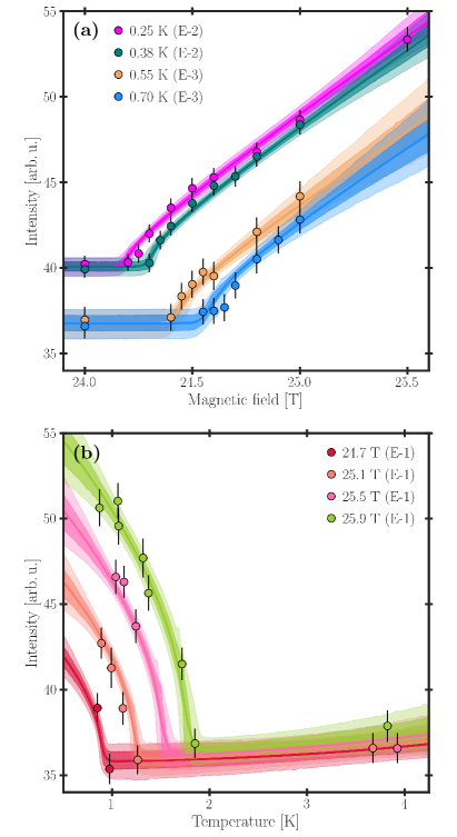
Figure 5: Peak intensities (symbols) extracted from the diffraction data. (a) Dependence of selected peak intensities on the applied magnetic field, shown for different constant temperatures. (b) Dependence on temperature displayed for different constant magnetic fields. Lines and shading show the mean (solid lines), 68% (light shading) and 95% (dark shading) credible intervals (CI) of the posterior distribution obtained from the global fit presented in Sec. IV.4.

Figure 5 displays the peak intensities extracted from the data (symbols) at constant temperatures [Fig. 5(a)] and at constant magnetic fields [Fig. 5(b)]. The temperatures quoted in Fig. 5(a) are the set values, whereas in Fig. 5(b) they are the actual sample temperatures taken from measurements made by the temperature sensor. In both panels, a large constant contribution is present due to nuclear scattering. In Fig. 5(a), the intensities increase sharply at a temperature-dependent value of the applied field where the ordered phase is entered. For fields just above the transition, this contribution is dominated by the transverse magnetization ($m_{\perp}$), while for higher fields the contribution of the longitudinal component ($m_{\parallel}$) becomes visible at 0.25 K and 0.38 K, causing the approximately linear dependence. In Fig. 5(b), the intensities decrease up to a field-dependent value of the temperature at which the ordered phase is left, with $m_{\perp}$ dominating the magnetic signal. In the thermally disordered phase, the rise in intensity with temperature is due to the contribution of thermally occupied $\ket{t^{+}}$ states to $m_{\parallel}$; at still higher temperatures, where the triplet states $\ket{t^{0}}$ and $\ket{t^{-}}$ also become thermally occupied, $m_{\parallel}$ would decrease again.

Clearly the functional form of the Bragg-peak intensity, and hence of the order parameter ($m_{\perp}$), does not follow a conventional form across the entirety of both panels in Fig. 5. However, before one could ascribe this situation to hallmarks of the unconventional physics depicted in Figs. 1(b) or 2(c), it is necessary to consider both the contribution of the longitudinal magnetization to the measured intensity and the likely width of the quantum critical scaling regime. To investigate this situation in a fully quantitative manner, while simultaneously making optimal use of the small number of data points at any given $\mu_{0}H$ or $T$, we construct a global model of the Bragg-peak intensities extracted from the diffraction data and compare its results to the conventional forms for the evolution of the order parameter.

IV.3 Peak-Intensity Model

Quite generally, the peak intensity can be modelled as

$$I^{\rm model}_{s}(H,T)=\mathcal{A}_{s}\Big{\{}n^{2}_{\perp}(H,T)+\mathcal{B}n^{2}_{\parallel}(H,T)\Big{\}}+\mathcal{C}_{s},$$ (1)

where $\mathcal{A}_{s}$ are experiment-dependent global scale factors and $\mathcal{C}_{s}$ are constant (spin-independent) contributions to the intensity, primarily due to nuclear scattering; here $s$ labels the three experiments (E-1, E-2, and E-3). $n_{\perp}$ is proportional to the transverse magnetization, $m_{\perp}$, and $n_{\parallel}$ is the triplon density, simulated by QMC in Ref. [Allenspach2020], which is proportional to the longitudinal magnetization, $m_{\parallel}$. $\mathcal{B}$ is an unknown factor governing the relative sizes of the two magnetic contributions, which depends on the specific magnetic Bragg peak under investigation and on the direction of the staggered transverse order.

The observed dependence of the peak intensities on both field and temperature [Figs. 5(a) and 5(b)] motivates an effective model for the $m_{\perp}$ contribution with the same scaling form as a typical order parameter,

$$\!\!\!\!n_{\perp}(H,T)= \enspace\Theta(g_{s}\mu_{B}\mu_{0}H-\Delta)\Theta(T_{c}(H)-T)$$

$$\enspace\times\bigg{[}\frac{g_{s}\mu_{B}\mu_{0}H\!-\!\Delta}{\Delta}\bigg{]}^{\kappa_{H}}\bigg{[}\frac{T_{c}(H)\!-\!T}{T_{c}(H)}\bigg{]}^{\kappa_{T}}\!\!\!,$$ (2)

where $\Theta(x)$ is the Heavyside function and $\Delta=3.15(3)$ meV is the spin gap determined from INS at zero field [Allenspach2020]. $g_{s}$ are the experiment-dependent g-factors that can be estimated from the alignment angles, $\zeta_{s}$, of the three experiments using

$$g_{s}=\sqrt{g_{cc}^{2}\cos^{2}(\zeta_{s})+g_{aa}^{2}\sin^{2}(\zeta_{s})}$$ (3)

with $g_{cc}$ = 2.306 and $g_{aa}$ = $g_{bb}$ = 2.050 [Zvyagin2006].

The shape of the phase boundary, $T_{c}(H)\propto T_{c}^{\rm QMC}(h)$, is known from QMC simulations based on the spin Hamiltonian determined by INS [Allenspach2020]. These simulations were performed by mapping the spin system to a system of hard-core bosons and with the field $h$ expressed in the same units as the interaction parameters (meV). To compensate for the $g$-tensor and for the discrepancy between the triplon and hard-core-boson dispersions, both the field and the temperature should be rescaled. We rescaled the field so that the effective gap of the hard-core bosons matched the INS gap, $\Delta$, and included one global scale factor for the temperature, $\alpha$, as an unknown model parameter, with which we modelled the phase boundary appearing in Eq. (2) as

$$T_{c}(H)=\alpha T_{c}^{\rm QMC}(g_{s}\mu_{B}\mu_{0}H).$$ (4)

Finally, the sample temperatures of the ($\mu_{0}H,T$) points, $\vec{T}\equiv\{T_{j}\}$ where $j$ labels all the points in Fig. 4(a), are included as parameters constrained by the mean and standard deviation of the temperature-sensor measurements.

To optimize the parameters of the peak-intensity model based on all of the measured data, we used a procedure of Bayesian inference (BI) to obtain the joint probability distribution, $p(\bm{\theta}|\mathcal{D})$, of these parameters, $\bm{\theta}\equiv(\kappa_{H},\kappa_{T},\alpha,\mathcal{B},\mathcal{A}_{s},\mathcal{C}_{s},\zeta_{s},\vec{T})$, where $\mathcal{D}$ denotes the data [Sivia1996; Bishop2006]. In BI, $p(\bm{\theta}|\mathcal{D})$ is referred to as the posterior distribution, and details of its definition and determination are in presented in Appendix A.

IV.4 Results of the Bayesian Inference Analysis

The parameter set $\bm{\theta}$ clearly contains a significant number of heterogeneous and interdependent variables, whose only common feature is that their effects within the model are well defined [Eq. (1)]. BI offers a powerful and systematic statistical procedure for solving this class of problem, i.e. for estimating the values of and quantifying the uncertainties in all of these interlinked parameters simultaneously, using the constraints set by experimental observation. By contrast, a piecewise or sequential method of separating out the contributions to Eq. (1) would risk introducing bias, propagating significant errors, and increasing the statistical uncertainties, particularly in a situation with limited experimental data. In the present case, one may summarize the goal of applying the BI procedure with such a global and simultaneous model as being to separate out the extrinsic uncertainties, which arose unavoidably in performing the experiment, from the intrinsic uncertainties arising from the imperfectly determined model parameters. In Appendix B we provide a detailed analysis to illustrate the dependence of the posterior distribution on the multiple parameters in the peak-intensity model, primarily by means of projections onto different parameter pairs.

Focusing first on the experimental parameters, the fact that the alignment angles in the three experimental runs may differ (Sec. IV.1) has an effect on the $g$-factor and as a result on the position of the phase boundary in ($\mu_{0}H,T$) space. From the posterior distribution we deduce that $\zeta_{\rm E-1}=22.3^{+0.9\,\circ}_{-0.9}$, $\zeta_{\rm E-2}=24.7^{+0.7\,\circ}_{-0.5}$, and $\zeta_{\rm E-3}=24.3^{+0.8\,\circ}_{-0.9}$. From these values we can conclude that our original alignment of the sample (22.5^∘) was accurate, but that either it was misaligned slightly during removal from the ³He cryostat and mounting on the dilution cryostat (E-2, E-3), or the alignment changed due to minor differences in the cryostats and their cold fingers. The change in $\zeta$ from E-2 to E-3 is likely the result of a strong quench of the magnet system that terminated E-2 and required maintenance of the entire system (before E-3). From these $\zeta$ values, the $g$-factors of the three experiments can be determined using Eq. (3) as $g_{\rm E-1}=2.271^{+0.003}_{-0.003}$, $g_{\rm E-2}=2.263^{+0.002}_{-0.002}$, and $g_{\rm E-3}=2.265^{+0.003}_{-0.003}$. Concerning the $\mathcal{A}_{s}$ and $\mathcal{C}_{s}$ parameters, we find broad consistency across each of the runs, indicating the internal consistency of the assumptions made in the global model.

Turning to the parameters of the physical model, we comment first that the maximum gain in accuracy compared to our previous study of criticality in Sr-doped BaCuSi₂O₆ [Allenspach2021] stems from the fact that $\Delta$ is fixed in Eq. (2), because this functional form makes all the other parameters extremely sensitive to the value of $\Delta$ [Allenspach2020]. In the present case this fixes the critical field, $H_{c1}$, up to the measurement accuracy of the angles, $\zeta_{s}$, determining $g$ in Eq. (3). For the exponents of $n_{\perp}(H,T)$, we find systematic fits to a single value $\kappa_{T}=0.26^{+0.05}_{-0.06}$ describing the $T$-dependence and a single value $\kappa_{H}=0.45^{+0.05}_{-0.05}$ describing the $H$-dependence. These results may be viewed as a slight surprise, given that the widths of our fitting regimes in both $T$ and $H$ far exceed the widths over which one might expect to identify critical behavior with the same functional forms. In the event that sufficient data were available within the critical regimes, one would expect these exponents to show an asymptotic approach to the critical values for order-parameter scaling of the 3D-XY universality class, $\beta_{T}=0.3689(3)$ [Campostrini2002] and $\beta_{H}=0.5$ (mean-field scaling) [Matsumoto2004], which correspond respectively to classical and quantum criticality. Although the widths of the associated critical regimes are non-universal and not known a priori, it is clear from the values we obtain for $\kappa_{T}$ and $\kappa_{H}$ that the data we have included in the analysis extend well beyond them. However, the long data-acquisition times per ($\mu_{0}H,T$) point in our experiments made it impossible to increase the point density in these regimes to attempt an experimental determination of $\beta_{H}$ and $\beta_{T}$. Nevertheless, our results do provide a clear picture of the requirements for overcoming this experimental challenge and the peak-intensity model of Eq. (2) could be used directly in any future investigation that seeks to determine these critical exponents.

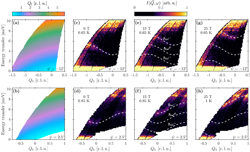
Figure 6: Dependence of the INS spectrum on magnetic field. (a,b) Representation of the dynamic range of scattering processes available on HFM/EXED in the space of $Q_{h}$, $Q_{l}$, and energy transfer ($\hbar\omega$) for sample alignment angles $\psi=-12^{\circ}$ (a) and $2.5^{\circ}$ (b). (c-h) TOF spectra measured on HFM/EXED for both values of $\psi$ at three different magnetic fields, reduced to the space of $Q_{h}$ and $\hbar\omega$ by integrating $Q_{l}$ over the range [0,8]; the integration range in $Q_{k}$ was [$-0.2$, 0.2] for all panels. Dashed white lines represent the average positions of the three Zeeman-split triplon modes, whose modelling is described in Sec. V.3.

For a quantitative discussion, the fit provided by the global peak-intensity model, using the parameters optimized by constructing the posterior distribution of BI, is represented in Fig. 5 by showing the mean intensities as the solid lines and the uncertainties as the 68% confidence interval (CI, dark shading) and the 95% CI (light shading). A small discrepancy visible at 0.7 K in Fig. 5(a) may be caused purely by statistical fluctuations, because the mean of the posterior is within the 68% CIs of all the peak intensities extracted at 0.7 K except for the one at 24.65 T. The temperature-dependence of the extracted peak intensities shown in Fig. 5(b) is described rather well below $T_{c}(H)$ by a single critical exponent [Eq. (2)], and thus within the sensitivity and counting statistics of the experiment it is not possible to observe any hallmarks of the special quasi-2D form of $m_{\perp}(T)$ illustrated in Fig. 1(b) [Furuya2016].

Turning to $m_{\perp}(H)$, although its low-temperature evolution at the higher fields in Fig. 5(a) is faintly suggestive of the unconventional forms illustrated in Fig. 2(c), it is not possible to exclude some more mundane reasons for these observations. Nevertheless, we note that the field $H^{*}$ determined by the B-bilayer interactions in BaCuSi₂O₆ [Allenspach2020] is 25.8 T, and thus it is possible that the maximum field available on HFM/EXED falls just short of the value required to reveal this type of behavior. While we can conclude that these effects are weak for the parameters (two-dimensionality and bilayer stacking) of BaCuSi₂O₆, we cannot exclude that they may be observable to the next generation of high-field neutron diffraction experiments, and thus they pose an open challenge to future facilities.

V Inelastic Neutron Scattering Measurements

V.1 Experimental Conditions

The magnetic excitations of BaCuSi₂O₆ have been measured by INS in the disordered phase at zero magnetic field [Sasago1997; Allenspach2020] and at fields up to 4 T [Rueegg2007]. Here we present INS measurements of the magnetic excitation spectrum up to the far higher field of 25 T made possible by using HFM/EXED in its spectroscopy mode. These were performed only during E-1, where the base temperature of 0.65 K was set by the ³He cryostat. An incoming neutron energy of $E_{i}=12$ meV and the associated chopper settings were selected to maximize the neutron flux in the energy-transfer range of the magnetic excitations. TOF spectra were measured for different magnetic fields from 0 T to 25 T using two different magnet rotations, $\psi=-12^{\circ}$ and $2.5^{\circ}$, which correspond to the minimal and maximal values of $\psi$ [Fig. 3(d)]. Measurements were performed at 0.65 K for 6 hrs at $\psi=-12^{\circ}$ for five magnetic fields (0, 10, 15, 20, and 25 T), but due to time constraints only three TOF spectra (at 0, 15, and 25 T) could be measured, each for 3 hrs, with $\psi=2.5^{\circ}$. At this $\psi$ value our measurements were performed at 0.85 K (0 and 15 T) and 1 K (25 T), which had no effect on the physics of the gapped spin system.

V.2 Measured INS Spectra

The measured INS data were preprocessed and transformed into energy-momentum space using the software Mantid [Arnold2014], normalized by the monitor and a vanadium standard, and the result was scaled by $k_{i}/k_{f}$ to provide the normalized intensities $I(\vec{Q},\omega)$. To improve the statistics, the data were integrated over $[-0.2,0.2]$ in $Q_{k}$, which corresponds to the direction perpendicular to the scattering plane.

In a conventional TOF measurement, the sample may be rotated through a wide angular range. Because of the need to fix the value of $\psi$ on HFM/EXED, the dynamic range of the $Q_{k}$-integrated data constitutes not a dense 3D subset of energy-momentum space but two 2D subsets that cannot be aligned with any high-symmetry directions. Thus accessing the full range of $\omega$ values requires sampling over a broad range of both $Q_{h}$ and $Q_{l}$. The $Q_{h}$- and $Q_{l}$-dependence of $\omega$ for the dynamic range of our measured TOF spectra is shown for the two $\psi$ values in Figs. 6(a) and 6(b). In BaCuSi₂O₆ it is known [Allenspach2020] that the important dispersion information is contained in the $(Q_{h},\omega)$ plane, with only minimal dependence on $Q_{l}$, and hence it is clear that visualizing the TOF spectrum as a function of $Q_{h}$ over an energy-transfer range covering the Zeeman-split triplon excitations up to 25 T requires integration over a very wide range of $Q_{l}$.

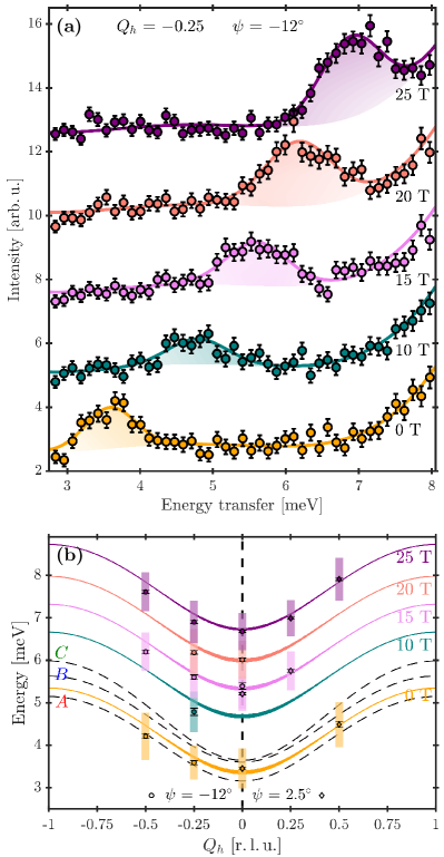
Figure 7: Field-induced evolution of the triplon spectrum. (a) Scattered intensity as a function of energy transfer, as extracted from the TOF spectra at fixed $Q_{h}$ and $\psi$, at all five applied magnetic fields; respective curves are offset by 2.5 [arb. u.] for clarity. Solid lines and shading show the results of the fitting procedure described in the text. (b) Measured average excitation energy of the upper triplon branch, shown as a function of $Q_{h}$ for the same five fields. Vertical colored bars indicate the widths of the Gaussian functions deduced from panel (a), expressed as their full width at half-maximum height. Black symbols indicate the mode energies, with error bars, extracted from the Gaussian center positions. Solid lines show the position of the composite (A+B+C) $\hbar\omega^{-}$ triplon mode, modelled as a weighted average intensity for each different field. The thicknesses of these lines indicate the effect of $Q_{l}$ on the dispersion. The dashed lines at $H=0$ show the dispersions of the A, B, and C triplons, whose separation explains the widths in energy of the observed intensity peaks. All data at $Q_{h}<0$ are for $\psi=-12^{\circ}$ and at $Q_{h}>0$ for $\psi=2.5^{\circ}$.

Figures 6(c)-6(h) show the spectrum in the plane of $Q_{h}$ and $\omega$ obtained by integrating the TOF data over the range [0,8] in $Q_{l}$. At zero magnetic field [Figs. 6(c) and 6(d)], only one excitation is visible because the inequivalent three triplon modes (A, B, C) observed in Refs. [Rueegg2007; Allenspach2020] cannot be resolved individually in the high-flux spectroscopy mode on HFM/EXED. The dashed white lines are taken from a model for a single composite mode, A+B+C, as detailed below. The spectra measured for $\psi=-12^{\circ}$ have better statistics than those measured at $\psi=2.5^{\circ}$ due to the longer data-acquisition time. An area of zero detector intensity, appearing close to $Q_{h}=0$ and extending to low but finite energies, is caused by the beam-stop, which blocks neutrons scattered in a certain angular range around the direct beam. Above 8 meV, non-dispersive and field-independent scattering can be observed for both $\psi$ values. This signal was not present in previous INS measurements performed on BaCuSi₂O₆ using other TOF spectrometers at zero field [Allenspach2020], but has been observed previously on HFM/EXED, and so we ascribe this known background feature to neutrons scattered by the cryostat, magnet, or sample holder. The finite scattered intensities close to the lower $Q_{h}$ boundaries of the dynamic range at all energies for the TOF spectra measured at $\psi=-12^{\circ}$ were also not observed in previous experiments and are thought to be artifacts of the integration over $Q_{l}$, which risks picking up the tails of a Bragg peak such as ($-2$ 0 2) or ($-2$ 0 4).

As an initial model for our spectral data, we will assume that the effect of the applied field is only to cause a Zeeman splitting of the three excited triplet states, $\ket{t^{-,0,+}}$. However, it has been shown for the quasi-1D spin dimer system BPCB that additional bound states can form between excited triplets and the condensed triplets that are present above $H_{c1}$ [Nayak2020], and below we comment on the possible applicability of such a scenario in BaCuSi₂O₆. For the triplets $\ket{t^{-,0,+}}$, the ratio of the transition probabilities, $p_{s}^{-,0,+}$, from the singlet ground state is given by $p_{s}^{-}\,$:$\,p_{s}^{0}\,$:$\,p_{s}^{+}$ = 1:2:1 [Rueegg2007]. Thus the Zeeman-split branch at energy $\hbar\omega^{0}$ is expected to have double the intensity of branches at $\hbar\omega^{-,+}$. The intensities of each of these modes are also proportional to the dimer structure factor, which in BaCuSi₂O₆ has the form $[1-\cos(2\pi Q_{l}d/c)]$, where $c$ is the lattice constant in the stacking direction [Fig. 2(a)] and $d$ the separation between the Cu²⁺ ions of the dimers [Allenspach2020]. One consequence of the dynamic range of HFM/EXED shown in Figs. 6(a) and 6(b) is that the upward shift of the $\hbar\omega^{-}$ branch caused by increasing the field also causes its intensity to increase, whereas the $\hbar\omega^{+}$ branch loses intensity as its energy decreases. Because the experimental statistics are not sufficient to distinguish the $\hbar\omega^{+}$ and $\hbar\omega^{0}$ branches from the $\omega$-dependent background at finite fields, in the following we focus on the analysis of the $\hbar\omega^{-}$ branch.

V.3 Field-Dependence of the Triplon Energy

Cuts from the TOF spectra of Figs. 6(c)-6(h) were extracted to deduce the scattered intensity as a function of $\omega$ by using an integration range of $[Q_{h}-0.1,Q_{h}+0.1]$ about each fixed $Q_{h}$ value. Figure 7(a) shows equivalent cuts for all five different magnetic-field values at fixed $Q_{h}$ and $\psi$. These cuts were fitted simultaneously over all $Q_{h}$ and both $\psi$ values by using an individual Gaussian for the excitation branch visible in each cut and a polynomial background that was shared for all the cuts at different magnetic fields; the resulting fits are represented by the solid lines and shading in Fig. 7(a).

The extracted mode energies, corresponding to the center positions of the fitted Gaussians, are displayed as black symbols in Fig. 7(b). The colored bar indicates the width of each Gaussian, which as expected from Fig. 7(a) is quite large, and the black symbols within each bar indicate the center position and the actual statistical error in its location. To interpret these fits, we have modelled the composite mode we observe, A+B+C, by taking an intensity-weighted sum of the individual triplon modes, with a Zeeman splitting appropriate to the applied field, using the interaction parameters determined at $H=0$ [Allenspach2020]. In this modelling procedure, the dependence of each individual mode ($\gamma\in{\rm A,B,C}$) on the field is described by the Zeeman term, $\pm g\mu_{B}\mu_{0}H$, for fields $H<H_{c1}$. Above $H_{c1}$, the new ground state is predominantly [Matsumoto2004] a superposition of $\ket{s_{\gamma}}$ and $\ket{t^{+}_{\gamma}}$ states on dimers in bilayers of type $\gamma$, so that modes $\hbar\omega^{0}_{\gamma}$ increase linearly in energy by $g\mu_{B}\mu_{0}(H-H_{c1})$ and modes $\hbar\omega^{-}_{\gamma}$ by $2g\mu_{B}\mu_{0}(H-H_{c1})$. Because all our inelastic measurements were performed directly after the diffraction experiments E-1, without any changes to the sample alignments, the $g$-factor determined in the diffraction analysis (Sec. IV), $g_{\rm E-1}=2.271^{+0.003}_{-0.003}$, was used to model the field-dependence of the triplon modes. $H_{c1}=\Delta/(g\mu_{0}\mu_{B})$ was obtained directly from the measured zero-field spin gap, $\Delta=3.15$ meV [Allenspach2020].

In Fig. 7(b) we apply this modelling process to the zero-field case in order to illustrate the extent of the differences between the modes A, B, and C. It is clear that the splitting of the three inequivalent triplon modes [Allenspach2020] is almost entirely responsible for the width of the intensity distributions appearing in Fig. 7(a). We comment that the effect of the wide integration over $Q_{l}$ in the quasi-2D BaCuSi₂O₆ system is extremely small by comparison, causing a broadening of the modelled dispersions that is at most 0.1 meV at $Q_{h}=0$. At finite fields, we observe that there are no significant changes either in the shape of the dispersive $\hbar\omega^{-}$ branch or in the widths of the fitting Gaussians and in the statistical uncertainties. We note that the dashed lines in Figs. 6(c)-6(h) show the modelled positions of the weighted average intensity peaks for the three branches $\hbar\omega^{-,0,+}$.

Thus the summary from our INS experiments is that the observed intensities are fully consistent with theoretical modelling based on Zeeman-split triplet modes over the full field range of the measurements up to 25 T, with no significant deterioration of data quality or fitting quality. Returning to the question of whether additional modes might appear in the spectrum around $H_{c1}$ as a result of bound-state formation, we comment that this type of physics is strongly favored by inter-dimer frustration [Nayak2020]. Recalling from the inset of Fig. 2(a) that the full magnetic Hamiltonian does contain moderately frustrated pairwise ionic interactions, it is certainly possible that bound states could be found in the spectrum of BaCuSi₂O₆ at $H>H_{c1}$. Such states are expected to appear as a splitting of the $\ket{t^{0}}$ and $\ket{t^{-}}$ modes at their upper band edge ($Q_{h}=\pm 1$ in Figs. 6 and 7), where unfortunately the absence of spectral weight at energy $\hbar\omega^{0}$ and the presence of background scattering at $\hbar\omega^{-}$ preclude any reliable identification. The possibility of observing field-induced bound-state formation in BaCuSi₂O₆ therefore remains as a further challenge to future high-field spectrometers.

VI Discussion and Conclusion

We have performed neutron diffraction and spectroscopy experiments on the quasi-2D spin-dimer material BaCuSi₂O₆ at magnetic fields up to 25.9 T using the TOF neutron scattering instrument HFM/EXED at the Helmholtz-Zentrum Berlin. With these applied fields we were able to access the phase of field-induced magnetic long-range order, in which we measured the nuclear and magnetic intensities of the ($-2$ 0 2) Bragg peak and the dispersion of the uppermost Zeeman branch of the triplon excitation spectrum. The diffraction data are well described by a global peak intensity model that is fully consistent with a conventional shape of the magnetic order parameter. The inelastic data, not previously obtainable by any technique, are also consistent with Zeeman-split triplon and magnon spectra modelled in both the quantum disordered and field-induced ordered phases on the basis of the interaction parameters extracted from zero-field INS [Allenspach2020].

Technically, the fact that INS measurements on BaCuSi₂O₆ had previously been performed up to only 4 T [Rueegg2007] means that HFM/EXED allowed an enormous breakthrough in neutron scattering capabilities. This improvement is both quantitative, in vastly increasing the splitting of the Zeeman branches of the spectrum, and qualitative, in accessing the order parameter of the field-induced magnetic phase. These results showcase the capabilities of HFM/EXED, particularly when combined with modern statistical methods for the analysis of limited experimental datasets. On this note, our results also exemplify the challenges intrinsic to performing measurements at such high magnetic fields, and offers some routes to overcoming these. As one example, the restricted scattering geometry set by the magnet design meant that rather long data-acquisition times were required in our experiments to obtain sufficient statistics both for the Bragg-peak intensities at each ($\mu_{0}H,T$) point and for the magnetic excitations at a specific magnet rotation. Nevertheless, these trials present invaluable input for assessing the factors generating maximum impact on the capabilities of next-generation high-field magnets at neutron sources.

Scientifically, BaCuSi₂O₆ remains a valuable target material for its potential to exhibit exotic behavior of both ground and excited states under high fields. As a system of stacked, inequivalent bilayer units whose non-uniform nature offers a strong enhancement of quasi-two-dimensionality, it presents the possibility to observe unconventional behavior of the order parameter as a function of either temperature or field. However, even with the 1:12 inter- to intra-bilayer interaction ratio determined in BaCuSi₂O₆, and with an enhancement factor of $J^{\prime\prime}/[J_{B}-J_{A}]\approx 1/10$ induced by the non-uniform stacking, the 3D coupling remains sufficiently strong that we could not detect an unconventional modification of the order parameter, of the types shown in Figs. 1(b) [Furuya2016] or 2(c). Although this spatial anisotropy may seem large, it provides a reference point for future investigations seeking to confirm the proposal of Ref. [Furuya2016] for quasi-2D magnetic systems. Our investigation broadens the scope of this search by underlining the importance of achieving non-uniform layered structures with larger energetic mismatches between the interactions in the different layers.

Appendix A Definition of the Posterior Distribution

The posterior distribution,

$$p(\bm{\theta}|\mathcal{D})\propto p(\mathcal{D}|\bm{\theta})p(\bm{\theta})$$ (5)

is constructed from the prior distributions, $p(\bm{\theta})$, of all the model parameters and the likelihood function, $p(\mathcal{D}|\bm{\theta})$. We start our definition of the prior distributions with the experiment-dependent rotations, $\zeta_{s}$, of the sample within the scattering plane, which were estimated from the positions of the Bragg peaks on the detector. These were gauged in turn using calibration measurements previously performed on HFM/EXED, yielding the estimates 22.7^∘ for E-1 and 24.1^∘ for E-2 and E-3, which were used as mean values for the prior probability distributions

$$p(\zeta_{1}) =\mathcal{N}(\zeta_{E-1}|\mu=22.7^{\circ},\sigma=1^{\circ})$$ (6)

$$p(\zeta_{2}) =\mathcal{N}(\zeta_{E-2}|\mu=24.1^{\circ},\sigma=1^{\circ})$$ (7)

$$p(\zeta_{3}) =\mathcal{N}(\zeta_{E-3}|\mu=24.1^{\circ},\sigma=1^{\circ}).$$ (8)

Here $\mathcal{N}(x|\mu,\sigma)$ denotes the normal distribution of $x$ with mean $\mu$ and standard deviation $\sigma$. We chose a standard deviation of 1^∘ to account for uncertainties arising from the out-of-plane misalignment, the field-dependent bend of the cryostat sample holder, and a possible offset in the magnetic-field direction of the magnet.

The constant intensity offsets, $\mathcal{C}_{s}$, do not include any magnetic contributions and are therefore independent of the magnetic field (in the absence of magnetostriction), as well as approximately temperature-independent for the temperature ranges measured on HFM/EXED. Thus we used the intensity extracted from the ($-2$ 0 2) peak at 15 T and 1 K measured in experiment E-2 as the mean of a normal prior distribution for $\mathcal{C}_{s}$,

$$p(\mathcal{C}_{s})=\mathcal{N}(\mathcal{C}_{s}|\mu=38.2,\sigma=10)\enspace\forall\,s.$$ (9)

The standard deviation of 10 was taken to allow for the fact that this mean intensity value was extracted from only one experimental ($\mu_{0}H$, $T$) point and because it includes a minor contribution due to the longitudinal magnetization, which is weak but not zero at 15 T and 1 K. For the other model parameters, we used a very broad normal distribution centered at 0 in order to effect an uninformative (i.e. unbiased) prior distribution,

$$p(\theta_{i})=\mathcal{N}(\theta_{i}|0,\sigma=1000),$$ (10)

where $\theta_{i}\in\{\kappa_{H},\kappa_{T},\alpha,\mathcal{B},\mathcal{A}_{s}\}$ and the units of $\sigma$ are the same as those of the parameters.

Regarding the uncertainties in the observables, as noted in Sec. IV.1 the accurate calibration of the magnetic-field values allowed us to neglect their uncertainties. The sample temperatures were estimated from the temperature-sensor measurements by taking the mean, $T^{\rm s}_{j}$, and standard deviation, $\delta T^{\rm s}_{j}$, of the time series obtained at each ($\mu_{0}H,T$) point, $j$. The actual sample temperatures, $T_{j}$, were then treated as unknown parameters (latent variables) using the prior distributions

$$p(T_{j})=\mathcal{N}(T_{j}|\mu=T^{\rm s}_{j},\sigma=\delta T^{\rm s}_{j})\enspace\forall\,j.$$ (11)

An alternative approach is to include the uncertainty in the sample temperatures as an extra factor in the likelihood function [Allenspach2021], which is mathematically equivalent to the procedure presented here. Assuming that the prior distributions of the individual peak-intensity model parameters, $\bm{\theta}=(\kappa_{H},\kappa_{T},\alpha,\mathcal{B},\mathcal{A}_{s},\mathcal{C}_{s},\zeta_{s},\vec{T})$, are independent, the joint prior distribution is given by

$$p(\bm{\theta})=\prod_{i}p(\theta_{i}).$$ (12)

The definition of the likelihood function is much more succinct. Using the peak intensities extracted from the data, $I^{\rm data}_{j}$, their error bars, $\delta I^{\rm data}_{j}$, and the peak-intensity model specified in Eq. (1)],

$$p(\mathcal{D}|\bm{\theta})=\prod_{j}\mathcal{N}(I^{\rm data}_{j}|\mu=I^{\rm model}_{j}(H_{j},T_{j}),\sigma=\delta I^{\rm data}_{j})$$ (13)

where $j$ labels the $(\mu_{0}H,T)$ points shown in Fig. 4(a), each of which was obtained from an experiment $s\in\{$E-1, E-2, E-3$\}$.

The posterior distribution was constructed by sampling from $p(\mathcal{D}|\bm{\theta})p(\bm{\theta})$. Because the peak-intensity model is continuously differentiable, Hamiltonian Monte Carlo (HMC) methods [Gelman2004; Bishop2006] can be applied and the specific method we used to obtain the posterior distribution was a Markov Chain Monte Carlo (MCMC) sampling scheme using a No U-Turn Sampler (NUTS) [Hoffman2014] implemented in the probabilistic programming Python package PyMC3 [Salvatier2016]. All the parameters of the peak-intensity model are positive quantities, but the performance of HMC methods is improved when sampling in unbounded parameter spaces, so instead of encoding this information by truncating the prior distributions at zero (for example with half-normal or truncated normal distributions), we used normal distributions and the absolute values of all the parameters. To assess the quality of the sampling, three independent chains were sampled and compared. After 5 000 tuning steps, we recorded 20 000 further steps and discarded the first 5 000 of these as ”burn-in” steps for each chain, thereby defining $p(\bm{\theta}|\mathcal{D})$ from a total of 45 000 samples.

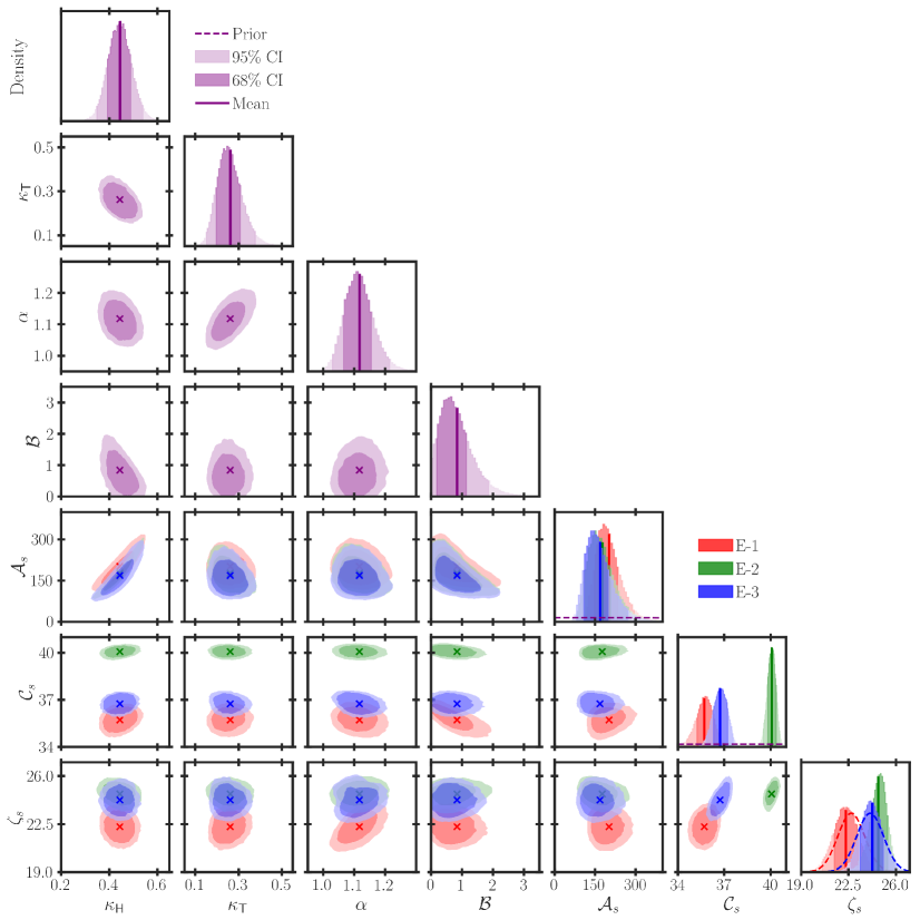
Figure 8: Projections of the joint posterior distribution of the peak-intensity model parameters [Eq. (1)]. Solid lines in the diagonal panels and crosses in the off-diagonal panels indicate the mean and shaded areas the 68% (dark) and 95% (light shading) CIs. The quantities dependent on each experiment, labelled using $s\in\{$E-1, E-2, E-3$\}$, are displayed in the three primary colors. Prior distributions of the model parameters (Appendix A) are shown as dashed lines, but are behind or below the horizontal axis in all cases other than $\mathcal{A}_{s}$, $\mathcal{C}_{s}$, and $\zeta_{s}$. For $\zeta_{s}$, the prior distribution is shown with the color code for each experiment, although the distributions for E-2 and E-3 coincide.

	Global	E-1	E-2	E-3
$\kappa_{H}$	0.45${}^{+0.05}_{-0.05}$
$\kappa_{T}$	0.26${}^{+0.05}_{-0.06}$
$\alpha$	1.12${}^{+0.04}_{-0.05}$
$\mathcal{B}$	0.8${}^{+0.3}_{-0.7}$
$\mathcal{A}_{s}$ [$\times 10^{2}$]		2.0${}^{+0.3}_{-0.5}$	1.8${}^{+0.3}_{-0.6}$	1.7${}^{+0.3}_{-0.6}$
$\mathcal{C}_{s}$		35.7${}^{+0.6}_{-0.5}$	40.1${}^{+0.3}_{-0.3}$	36.7${}^{+0.5}_{-0.4}$
$\zeta_{s}$ [∘]		22.3${}^{+0.9}_{-0.9}$	24.7${}^{+0.7}_{-0.5}$	24.3${}^{+0.8}_{-0.9}$

Table 1: Parameters of the peak-intensity model [Eq. (1)] inferred using Bayesian inference. Estimates are taken from the mean of the posterior distribution and their uncertainties from the differences between the mean and the 68% CI boundaries.

Appendix B Investigation of the Posterior Distribution

To characterize the multi-variable joint posterior distribution, in the diagonal panels of Fig. 8 we show its projections onto the space of a single model parameter, known as the marginal distributions, and in the off-diagonal panels we show projections onto pairs of parameters. The parameter estimates and uncertainties are determined from the mean and 68% CI boundaries of the marginal distributions and are listed in Table 1. Because the marginal distributions are unimodal, the Highest Posterior Density intervals [Gelman2004] are used as the CIs.

For all three of the physical model parameters, $\kappa_{H}$, $\kappa_{T}$, and $\alpha$, the marginal distributions show a well-defined single peak, with one characteristic width, and are only weakly skewed. For $\mathcal{B}$, the marginal distribution extends to very small values, with the lower 95% CI boundary at only 0.00025, but also displays a heavy tail towards larger values. To distinguish the experimental parameters unique to each run (E-1, E-2, or E-3), the marginal distributions of $\mathcal{A}_{s}$, $\mathcal{C}_{s}$, and $\zeta_{s}$ are shown using different colors. For $\mathcal{A}_{s}$, the entire marginal distributions of E-2 and E-3 overlap closely, but deviate slightly from E-1; these minor differences are most likely a result of different levels of neutron absorption in the two different cryostats. The marginal distributions of $\mathcal{C}_{s}$ are similar for E-1 and E-3 but differ for E-2, a 9% discrepancy (Table 1) already visible in the extracted peak intensity (Fig. 5). The coefficients $\mathcal{C}_{s}$ include not only the nuclear scattering contribution but also any other contributions that are constant in temperature and magnetic field, including any remnants of the background that might be added to the peak intensity in error when extracting it from fits to the ($-2$ $Q_{k}$ 2) cuts of Fig. 4. Finally, the marginal distributions of $\zeta_{s}$ are similar for E-2 and E-3 but differ from E-1, as discussed in Sec. IV.4. As one measure of the effectiveness of the BI procedure, the prior uncertainties of the model parameters are clearly reduced in every case other than the $\zeta_{s}$, because their prior distributions were chosen based on strict constraints imposed by the refinement of the peak position on the detector. Although these prior distributions are as a result informative, the (marginal) posterior distributions of $\zeta_{s}$ become narrower and their mean positions are nevertheless shifted due to the additional information provided by the extracted peak intensities.

Finally, the pair projections shown in the off-diagonal panels of Fig. 8 reveal any correlations between the parameters of the model. $\kappa_{H}$ and $\kappa_{T}$ show a weak negative correlation, while $\kappa_{H}$ is negatively correlated with $\alpha$ and $\kappa_{T}$ has a stronger positive correlation. $\mathcal{B}$ has a weak negative correlation with $\kappa_{H}$ but is almost independent of $\kappa_{T}$ and $\alpha$. The correlations of any of these parameters with an $s$-dependent parameter have the same form for all $s$. Other than a strong positive correlation of $\mathcal{A}_{s}$ with $\kappa_{H}$ and a negative correlation with $\mathcal{B}$, the remaining pair projections reveal no remarkable trends, from which one may surmize that the peak-intensity model both provides a meaningful account of the underlying physics and is robust against possible artifacts arising from the treatment of the experiments and data.