2022
[1]\fnmJulia A. \surMeister
[1]\orgdivComputing and Maths Division, \orgnameUniversity of Brighton, \orgaddress\cityBrighton, \postcodeBN2 4GJ, \stateEast Sussex, \countryUnited Kingdom
2]\orgnameDistributed Analytics Solutions, \orgaddress\street17 Fawe Street, \cityLondon, \postcodeE14 6FD, \countryUnited Kingdom
3]\orgdivDepartment of Computer Science, \orgnameRoyal Holloway University of London, \orgaddress\cityEgham, \postcodeTW20 0EX, \stateSurrey, \countryUnited Kingdom
A novel Deep Learning approach for one-step Conformal Prediction approximation
Abstract
Deep Learning predictions with measurable confidence are increasingly desirable for real-world problems, especially in high-risk settings. The Conformal Prediction (CP) framework is a versatile solution that guarantees a maximum error rate given minimal constraints shafer2008tutorial . In this paper, we propose a novel conformal loss function that approximates the traditionally two-step CP approach in a single step. By evaluating and penalising deviations from the stringent expected CP output distribution, a Deep Learning model may learn the direct relationship between the input data and the conformal p-values. We carry out a comprehensive empirical evaluation to show our novel loss function’s competitiveness for seven binary and multi-class prediction tasks on five benchmark datasets. On the same datasets, our approach achieves significant training time reductions up to 86% compared to Aggregated Conformal Prediction (ACP, norinder2016conformal ), while maintaining comparable approximate validity and predictive efficiency.
keywords:
Prediction confidence, Deep Learning, Conformal Prediction1 Introduction
How confident are Deep Learning predictions? In most cases, we assume that a model performs as well on new data as it has on average in the past rechkemmer2022confidence ; zhang2021confidence ; meister2022audio ; yin2019understanding . The Conformal Prediction (CP) framework presents an enticing alternative, providing per-prediction confidence based on statistical hypothesis testing vovk2005algorithmic . Given a user-specified significance level, standard CP guarantees a corresponding maximum error rate with more relaxed assumptions than commonly assumed in Deep Learning shafer2008tutorial . However, guaranteed absolute validity comes with computational efficiency drawbacks, making CP in its original form unrealistic for large-scale datasets riquelme2019coreset .
Several proposals have been made in recent years that successfully address CP challenges, although they tend to introduce a trade-off with other model characteristics linusson2017calibration . For example, inductive variants remove the need for repeated leave-one-out training papadopoulos2007conformal . Aggregated CP (ACP) improves predictive efficiency (i.e., the precision of the predictions), at the cost of training multiple ensemble models and losing absolute validity norinder2016conformal . However, to the best of our knowledge, such approaches maintain the underlying two-step CP algorithm: calculating data strangeness with an intermediate non-conformity measure, and subsequently transforming scores into p-values.
Distribution approximation provides an interesting avenue to address challenges related to the two-step nature of the Conformal Prediction algorithm. In this paper, we propose a one-step CP approximation approach with a novel, model-agnostic conformal loss function. By evaluating the deviation of the model output from the expected output distribution, we may circumvent the algorithmic constraints of the CP framework. Deep Learning is especially promising for this approach because the model’s versatility and potential to model complex data relationships is well-established lecun2015deep ; maskara2019advantages ; khatri2019prediction .
1.1 Contributions
To extend CP usability on real-world datasets, we make the following contributions:
-
•
We propose a unique loss function that approximates traditional two-step CP in only one step (Sections 2 and 3).
By enabling a Deep Learning (DL) neural network to learn the direct relationship between input data and the conformal p-values, we may skip the intermediate non-conformity scores altogether. -
•
We carry out a rigorous and comprehensive evaluation of our proposed method for 7 binary and multi-class classification tasks on 5 benchmark datasets (Section 4).
Empirical analysis of DL models trained with our loss function confirms competitiveness with Aggregated Conformal Prediction (ACP) in terms of approximate validity and predictive efficiency. However, our model is significantly more computationally efficient than ACP. -
•
Finally, our one-step approach to CP approximation introduces new opportunities for CP improvement (Section 5).
By modelling the expected output distribution directly, our novel loss function approach circumvents current CP algorithmic constraints. This is of particular research interest, as CP performance optimisation is traditionally a challenging task due to the interactions between the underlying model and the non-conformity measure cherubin2021exact .
The code and results described in this article are available in a GitHub repository111https://github.com/juliameister/dl-confident-loss-function.
2 Conformal Prediction
This section outlines the CP background, which the article builds on.
2.1 Background
The CP framework answers a ubiquitous question in Machine Learning: How confident are we that a model’s prediction is correct? In this article, the focus lies on a computationally efficient variant, Inductive Conformal Prediction (ICP) vovk2012conditional . Interested readers may refer to vovk2005algorithmic for a detailed description and context of the original transductive approach (TCP).
Under minimal data assumptions, CP provides guaranteed confidence for individual predictions, based on statistical hypothesis testing (shafer2008tutorial, ). Specifically, it guarantees that a predictor makes errors only up to a maximum user-specified error rate if the input data is exchangeable gupta2022nested . CP achieves this by outputting prediction sets with all plausible labels for classification problems (interested readers may refer to johansson2014regression for regression). An error occurs when the true label is not included in the CP prediction set . By the law of large numbers, the probability of an error occurring approaches the upper limit as the number of predictions grows (Equation 1), subject to statistical fluctuations fisch2021few .
| (1) |
In short, the CP framework acts as a wrapper for any prediction model, also called the underlying model lofstrom2013effective . Predictions are transformed into p-values that describe the likelihood of sample ’s extension with each possible label , denoted . The computationally efficient inductive CP variant (ICP) requires three sub-datasets. Let the proper training set be , the calibration set , and the test set . For each sample extension , the ICP model first evaluates how strange it is compared to the known training data norinder2017binary . The extension’s ‘strangeness’, or non-conformity, is measured with a score as a function of the extended sample and its true label . An example of a straightforward but versatile non-conformity measure (NCM) is the Margin Error function , given in Equation 3. A non-conforming example has a low probability estimate for the true label , and/or a high probability estimate for the false label johansson2017model .
| (2) | |||
| (3) |
For ICP, the model is fit to the data just once johansson2013conformal . This includes training the underlying algorithm with the proper training set , and calculating the NCM scores for the calibration set . Given a test score , we calculate the p-values for each , as shown in Equation 4. The numerator is also known as a ‘rank’. The larger the rank, the larger the p-value is, and the more conforming a sample extension is, compared to the training and calibration sets vovk2013transductive . Furthermore, Equation 4 guarantees that all p-values corresponding to the true labels are uniformly distributed in angelopoulos2020uncertainty .
| (4) |
Finally, given a test sample’s p-values , its CP prediction set is obtained with Equation 5. The optimal and most precise CP classification output is a prediction set with exactly one class label.
| (5) | |||
| (6) |
Note that, since the error rate and its inverse accuracy are automatically guaranteed by the validity characteristic, CP performance evaluation is traditionally based on predictive efficiency, i.e., prediction set size krstajic2021critical . Section 4.3 discusses metrics that may be used to evaluate CP performance.
2.2 Related work in conformal validity approximation
Optimising CP for both classification and regression tasks is an active research area sesia2021conformal ; papadopoulos2011regression ; linusson2021nonconformity because the framework has promising applications in high-risk, confidence-sensitive settings. CP is versatile, and a small selection of use cases include pharmaceutical drug discovery eklund2015application , respiratory health monitoring meister2020conformal ; nguyen2018cover , and financial risk prediction wisniewski2020application .
Since prediction accuracy is automatically guaranteed for traditional ‘full’ or Transductive CP (TCP), the primary optimisation objective is to increase predictive efficiency by outputting more precise prediction ranges (Section 2.1). Unfortunately, optimisation is a difficult task. There are two related but sometimes conflicting steps which must be considered simultaneously: the calibration of the underlying predictive model and the non-conformity measure. While promising approaches have been proposed that take both steps into account cherubin2021exact ; makili2013incremental ; papadopoulos2009reliable , they tend to be specific to certain underlying models and not generally applicable.
Additionally, TCP has computational efficiency challenges built into the algorithm and is not scalable to large, real-world datasets riquelme2019coreset . CP variants that address the inefficiency of the transductive leave-one-out retraining approach tend to accept a trade-off with other limitations linusson2017calibration . For example, Inductive Conformal Prediction (ICP) trades predictive efficiency for increased computational efficiency papadopoulos2007conformal .
In contrast, Aggregated Conformal Prediction (ACP) improves predictive efficiency by limiting prediction set sizes norinder2016conformal . It is a generalisation of previously proposed CP variants (Cross-conformal and Bootstrap conformal predictors, introduced in vovk2015cross ), inspired by ML prediction ensembles to reduce variance. For each test sample and possible label , the intermediate p-values generated by ensemble models are aggregated into one ACP p-value (e.g., with Equation 7, carlsson2014aggregated ). The intermediate p-values are calculated as shown in Section 2.1.
| (7) |
However, more precise ACP predictions come at the cost of losing automatic validity. While exact validity may be achieved with more stringent requirements or for some underlying models, approximate validity is observed empirically wilm2020skin . In particular, ACP tends to be conservative for low significance levels and invalid for high significance levels, because p-values close to the mean tend to be more common linusson2017calibration . There have been some effective proposals to recover validity solari2022multi ; toccaceli2019combination ; balasubramanian2015conformal , but these approaches do not address the significantly increased training times for multiple ensemble models compared to one ICP model.
In a recent and particularly relevant work, non-conformity scores were directly approximated by estimating their influence on the underlying model’s loss with Influence Functions (abad2022approximating, ). The purpose was to make the algorithm scalable to large datasets. The method successfully achieves validity on par with TCP, while removing the need for a leave-one-out training procedure for every test point. As the number of training samples increased, the authors observed an increasingly diminishing approximation error. In empirical experiments, the error became negligible at 10,000 training samples.
This confirms that validity and improved computational efficiency are possible by approximating individual steps of the TCP algorithm. In this article, we propose a novel conformal loss function that approximates the entire TCP two-step procedure by teaching a Deep Learning model the direct relationship between input data and conformal p-values.
3 Approximating conformal p-values directly with Deep Learning
Deep Learning (DL) is a highly versatile framework that automatically identifies and learns relationships between input data and output data, by extracting informative data representations lecun2015deep . A neural network with weights is made up of one or more hidden and interlinked layers (Equation 8). Each hidden neuron in a layer performs a simple linear transformation on the incoming data vector with weight vector , offset by an absolute bias , as shown in Equation 9 (ghalambaz2011hybrid, ). An activation function (e.g., ReLU) may then be applied to model non-linear data relationships.
| (8) | |||
| (9) |
Supervised training may be considered as an optimisation function with which the model attempts to minimise the deviation of its current output prediction to the expected output label olive2018supervised . For DL models trained with gradient descent, the difference between them is quantified via a loss function (Equation 10).
| (10) |
The loss is then back-propagated through the model. In Equation 11, each weight is updated with in proportion to its negative gradient (lillicrap2020backpropagation, ), reducing the output’s deviation from the true labels in the next iteration.
| (11) |
Once training is complete, a well-calibrated model will have optimised its learned weights so that Equation 8 accurately reflects the relationship between the input and its expected output label.
DL’s versatility and ability to represent complex data relationships make it a promising choice to model conformal p-values directly from the input, skipping the non-conformity scores (see Section 2). We hypothesise that a function composition of the two standard CP transformation steps (from data input to non-conformity measures, and from non-conformity measures to p-values) could be approximated with a suitably designed and trained model. In other words, the right DL architecture and loss function may be able to model the complex relationship between the input and conformal p-value output directly.
DL architectures have been used in the past to predict probability distributions of the target variable, e.g., with Mixture Density Networks makansi2019overcoming ; li2019generating ; zhang2020improved . However, to our knowledge, there is currently no model architecture (e.g., activation function) or loss function that can guarantee a uniform model output distribution, which is required for true-class conformal p-values (Section 2.1). Therefore, we propose an architecture-agnostic conformal loss function which ensures that the model output approximates the uniform distribution .
The purpose of our novel loss function is to achieve approximate validity and high precision, while significantly reducing the high algorithmic and computational complexity of similar CP variants. For example, ACP uses an ensemble approach to improve predictive efficiency norinder2016conformal . However, as the number of ensemble models grows, computational time increases significantly. Additionally, approximate validity becomes weaker because the distribution of aggregated p-values shifts away from (e.g., to a unimodal Bates distribution with the aggregation procedure shown in Equation 7) linusson2017calibration .
In contrast, a single DL model with our proposed conformal loss function is competitive with ACP up to 10 ensemble models in terms of approximate validity and high predictive efficiency, while significantly reducing algorithmic complexity and training time. Sections 3.1 and 3.2 describe the background and components of our proposed method in detail, and Section 4 provides a rigorous empirical evaluation of our results on the well-established MNIST datasets lecun1998gradient .
3.1 Proposed method requirements and constraints
This article’s contribution is to develop a unique conformal loss function for Deep Learning (DL). The novelty of our approach is that we simplify the two-step CP algorithm (Section 2) to only one step. Our loss function approximates conformal p-values directly from the input data, skipping the intermediate non-conformity measure. Therefore, the neural network’s output should follow the same distribution requirements as CP p-values:
-
•
To interpret the neural network output as conformal p-values, predictions should fall in the range (0, 1), and class outputs for one sample should be independent (Section 2.1).
-
•
To ensure validity and consequently a guaranteed error rate, approximated p-values of the true class should be uniformly distributed in linusson2017calibration .
-
•
To maintain high predictive efficiency, false-class approximated p-values should be close to 0 shafer2008tutorial .
Additionally, we must work within the constraints enforced by DL:
-
•
The loss function should be differentiable for effective backpropagation with gradient descent lecun2015deep .
-
•
The trade-off between model genralisability (small batch size, kandel2020effect ) and output distribution evaluation precision (large batch size, hao2019doubly ) should be considered.
3.2 Proposed conformal approximation loss function and background
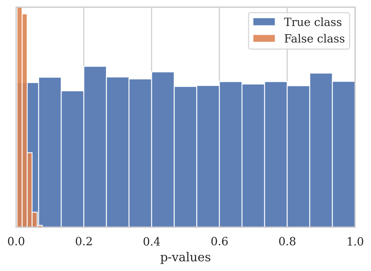
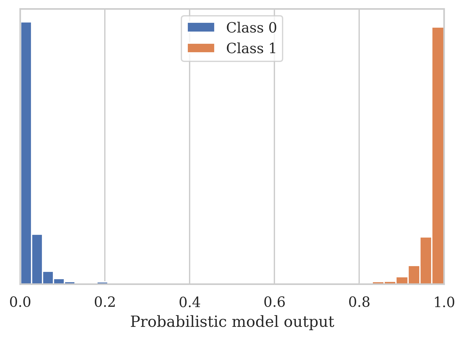
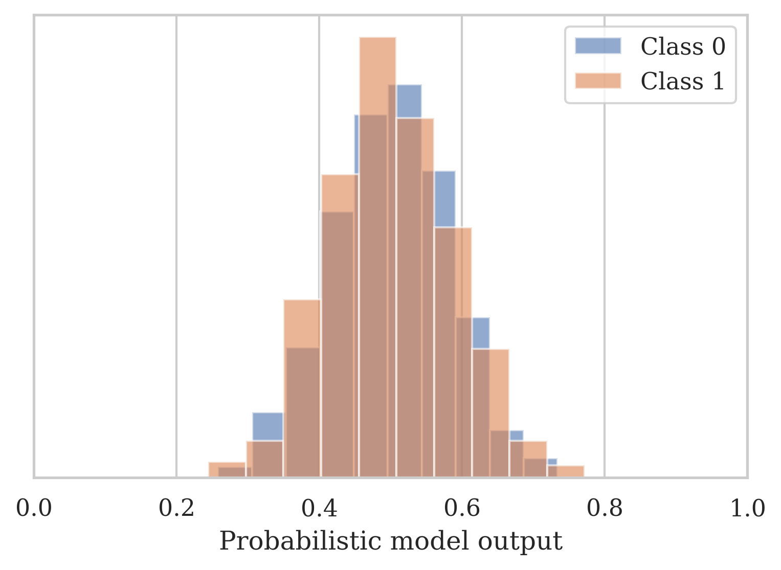
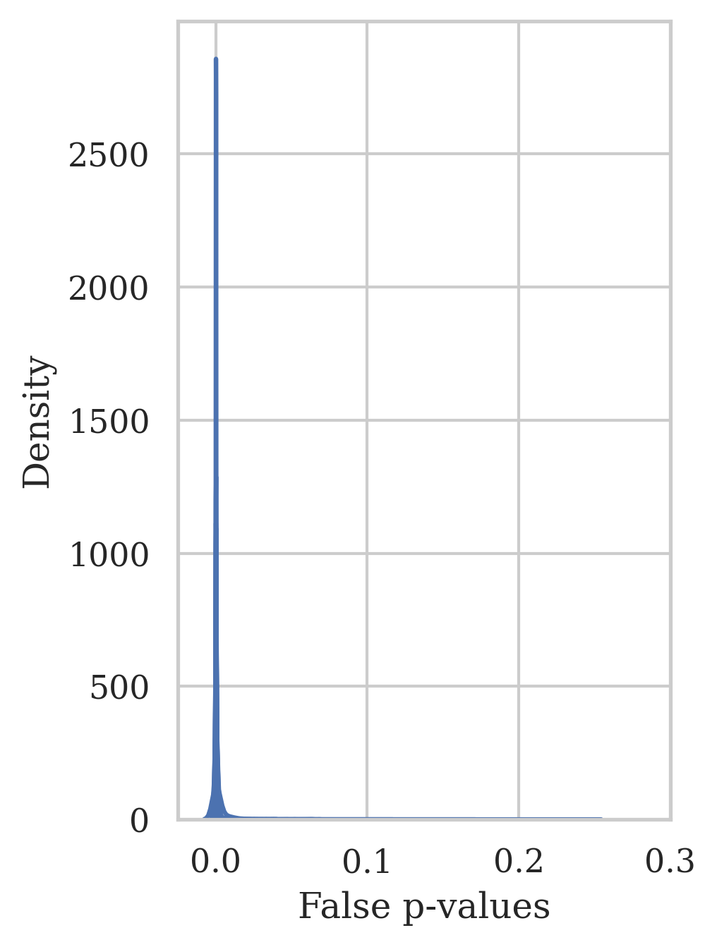
To approximate conformal p-values directly from the input data, we propose a conformal loss function that is compatible with a probabilistic, binary classification neural network (architecture details in Section 4). Given the requirements of the CP framework (Section 2), we know that well-calibrated CP classifiers are marked by a uniform distribution of the true-class p-values, and a distribution peaking at 0 with little variance for false-class p-values linusson2017calibration , as visualised in Figure 1(a). In contrast, typical well-calibrated neural network (NN) classifiers have a distinctive maximum distance between true-class (peak at 1) and false-class (peak at 0) output distributions, as shown in Figure 1(b). The challenge for the conformal loss function is to accurately describe the CP output distribution, so that the neural network may emulate it, avoiding the normal-like distribution that tends to occur when under-fit models make average random guesses (Figure 1(c)). Therefore, we propose a loss function that is made up of two components, optimising the true-class and false-class target distributions, respectively:
| (12) |
Since approximated p-values of the false class should follow the same pattern as traditional NN false-class predictions, we calculate standard Binary Cross Entropy (BCE) to minimise the values towards 0. Equation 13 defines BCE as a function of the model’s predictions and the true labels for training samples (ho2019real, ). For the purpose of the conformal loss function, we calculate BCE only for the false-class approximated p-value predictions (Equations 14 and 15).
| (13) | |||
| (14) | |||
| (15) |
Unlike traditional classification, the true labels are not the target model output in CP. Instead, true-class predictions (Equation 16) should follow the distribution over samples (Section 2). As a consequence, the loss component should evaluate and quantify the distance of the model output distribution from the target uniform distribution, rather than the distance to a concrete label per sample. Note that the trade-off between large sample counts for distribution estimation jaki2019effects and small batch sizes for optimised learning kandel2020effect must be carefully considered.
Even though function moments do not necessarily uniquely characterise a distribution, they may be a sufficient heuristic for a distribution distance evaluation malz2018approximating . Lower order moments require fewer samples to estimate and are therefore suitable for the proposed true-class conformal loss component, shown in Equation 10. When is minimised, the distribution of approximates . In Section 4, we empirically confirm that our one-step approximation approach is competitive with ACP in terms of uniformity and predictive efficiency, and significantly improves the computational efficiency.
| (16) | |||
| (17) |
Including the mean of true-class model outputs ensures that the output distribution is centred around 0.5 (Equation 19). Because model training minimises the overall loss, we square and take the root, so that any deviation is represented by a positive value. A larger value indicates a greater distance between the model’s output distribution and the expected mean of the uniform distribution .
| (18) | ||||
| (19) |
Similarly, for the variance , the component regulates the dispersion of so that it matches the expected value .
| (20) | ||||
| (21) |
To measure uniformity while maintaining differentiability (i.e., without ranking or sorting), we leverage the work in batu2017generalized . The authors suggested that for an unknown distribution, measuring sample collisions with moments (such as -norms) was a successful approximation for uniformity testing.
We choose the -norm as our heuristic, since it is fully differentiable and sensitive to outliers, i.e., it will penalise large differences more than smaller ones (meyer2021alternative, ). In Equation 23, is normalised to ensure that minimising the loss component increases the uniformity of the model output distribution. Note that does not necessarily measure uniformity in the range , only the distribution probability’s smoothness between the input vector’s extreme elements. The distribution’s mean, variance, and the next loss component counteract this drawback by encouraging values throughout the entire range.
| (22) | |||
| (23) |
Traditionally, Huber loss (Equation 24) is used to narrow the prediction region to the true label. In Equation 25, we negate the value instead to disincentivise the trend to normal-like distributions on the average output of under-fit models. The parameter regulates the threshold for the transition between quadratic and linear (meyer2021alternative, ). Since the target distribution for is , we expect the over-represented prediction to be (see Section 4). As with previous loss components, Huber loss is fully differentiable and robust to outliers.
| (24) | |||
| (25) |
Algorithm 1 illustrates how the described loss components come together to produce our novel conformal loss function (also shown in Equation 10). The function is fully differentiable and, therefore, may be used in combination with any backpropagation model. All individual evaluation metrics are inbuilt into tensorflow, meaning that our proposed loss is compatible with any tensorflow model. Algorithm 2 shows the Python 3.9 implementation as a tensorflow v2.4 custom loss function.
4 Empirical results
This section comprehensively evaluates the empirical performance of our proposed one-step conformal loss function (Section 3.2). In particular, we compare the validity, predictive, and computational efficiency to the well-established ACP approximation technique (Section 2.1) for both binary and multi-class classification on 5 benchmark datasets.
4.1 Research questions
The following research questions informed and structured the performance evaluation of our novel conformal loss function:
-
•
Can we directly model the relationship between the input data and the conformal p-values, skipping the intermediate non-conformity measure?
-
•
Is our proposed approach competitive with the established ACP approximation in terms of validity and predictive efficiency?
-
•
What benefits may approximating CP with a single-step approach have, compared to the traditional two-step calculations?
4.2 Datasets
We rigorously evaluate our proposed method for 7 classification tasks on 5 benchmark datasets. Predetermined train-test splits that were stored in the datasets were maintained. All other datasets are split into 67% training and 33% test samples, stratified by class. To reduce spurious noise in the results, the same split was used for all test runs. Sample counts are provided in Table 1.
| Samples | MNIST2 | MNIST10 | USPS2 | USPS10 | WINE | BANK | MSHRM |
|---|---|---|---|---|---|---|---|
| Train | 12,665 | 60,000 | 2,199 | 7,291 | 4,352 | 27,595 | 40,916 |
| Test | 2,115 | 10,000 | 623 | 2,007 | 2,145 | 13,593 | 20,153 |
| 14,780 | 70,000 | 2,822 | 9,298 | 6,497 | 41,188 | 61,069 |
4.2.1 MNIST dataset
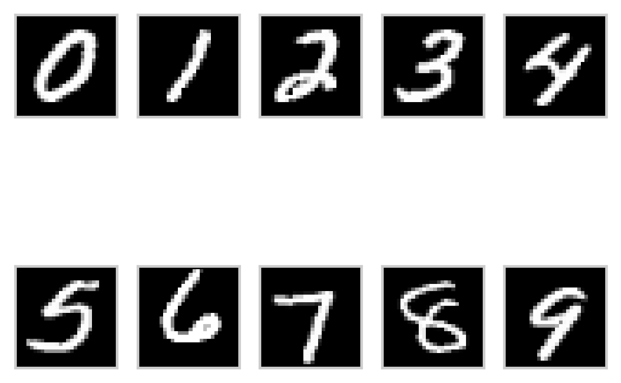
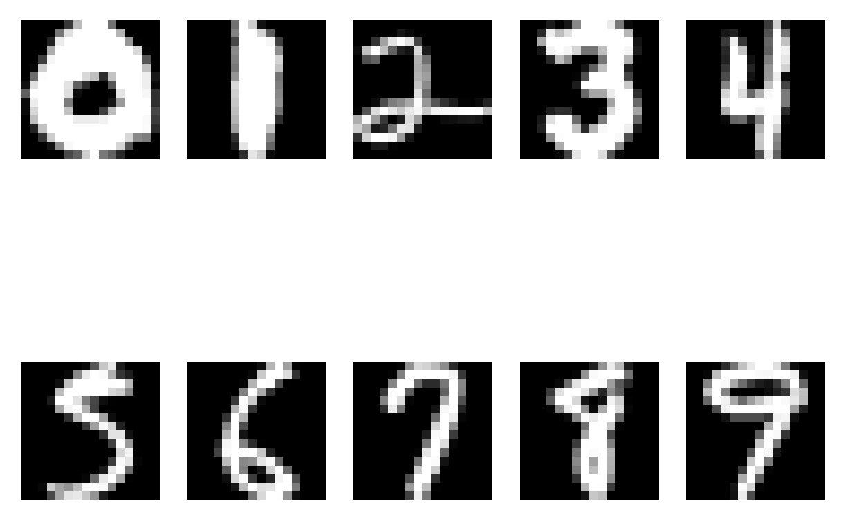
The MNIST dataset is an extensive collection of 70,000 images, each with a handwritten digit between 0–9 lecun1998gradient . The greyscale images are formatted as 28x28 binary vectors (see Figure 2(a)), flattened to (781 x 1) since we work with a linear feedforward network (see Section 4.4). We evaluate our proposed method for both binary classification (images of 0 and 1, referred to as MNIST2) and multi-class classification with all 10 digits (referred to as MNIST10). The classes are roughly balanced.

4.2.2 USPS dataset
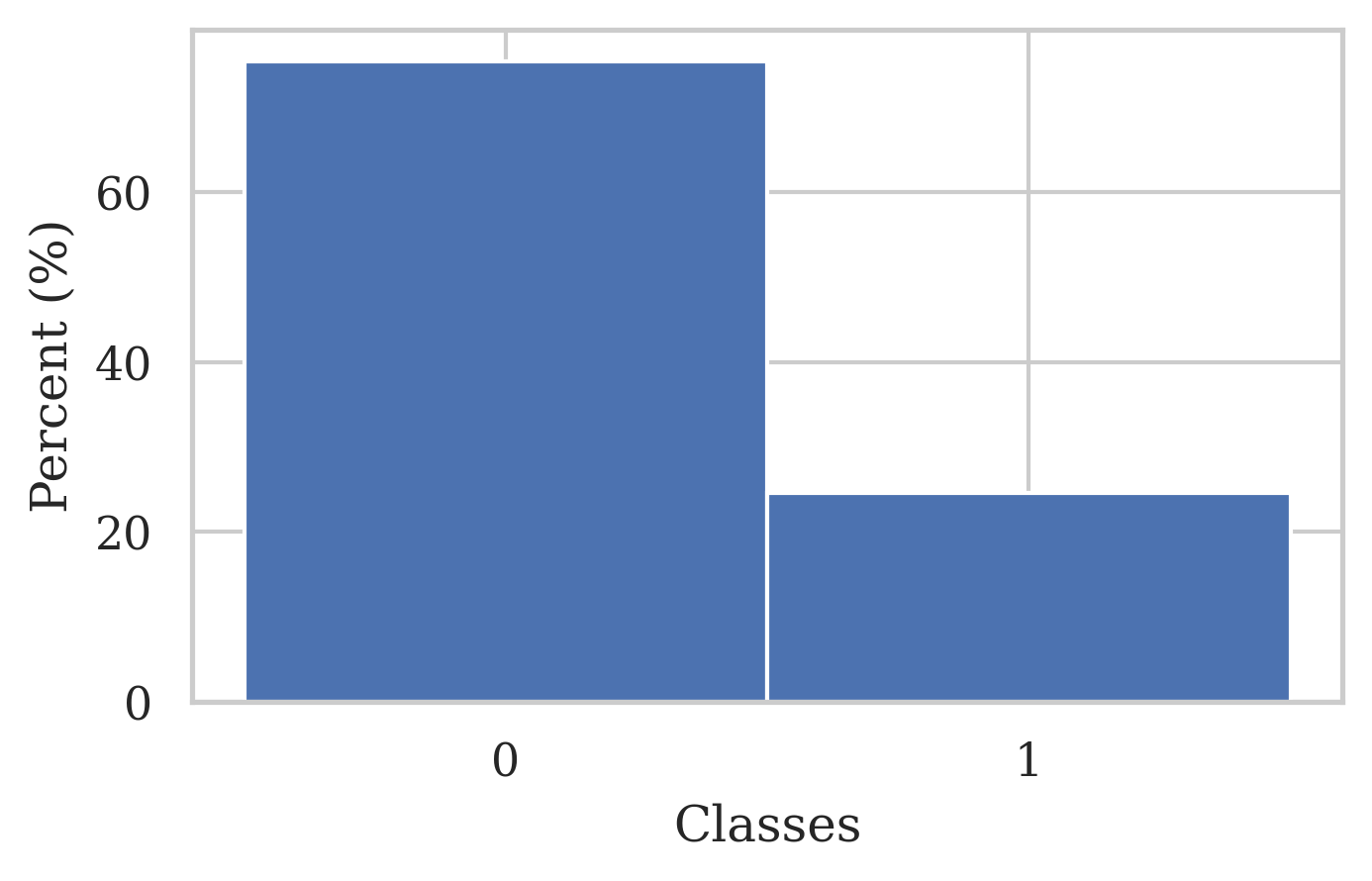
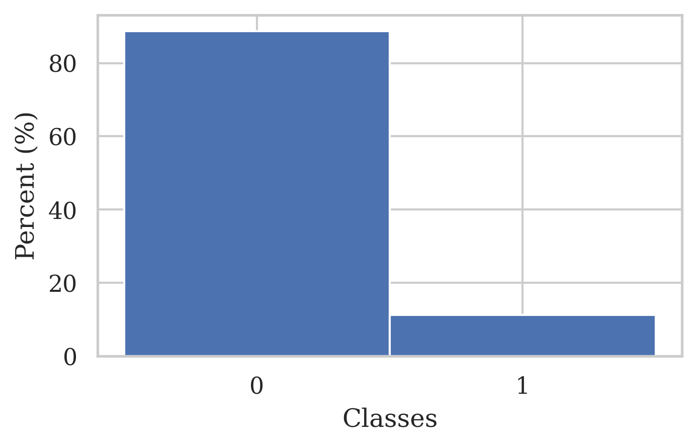
The USPS dataset is a collection of handwritten digits in greyscale, collected from envelopes by the US postal service hull1994database . The images come in (16x16) images that are flatted to (256 x 1) feature vectors. Similarly to the MNIST dataset in Section 4.2.1, we consider two classification tasks: binary (USPS2) and multi-class (USPS10). Examples and the class distribution are visualised in Figure 3.

4.2.3 Wine dataset
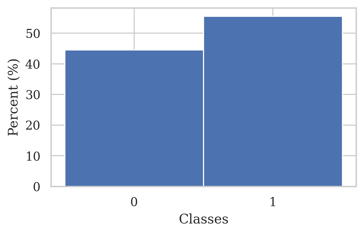
We use the Wine dataset to distinguish between red (class 1) and white (class 0) wines. We use 11 of the 12 features: Fixed acidity, volatile acidity, citric acid, residual sugar, chlorides, free sulphur dioxide, total sulphur dioxide, density, pH, sulphates, and alcohol. Wine quality is excluded because it is heavily imbalanced between the two classes. Readers are referred to CorCer09 for detailed information about the features and Figure 4 for the class distribution.
4.2.4 Bank marketing dataset
The Bank marketing dataset contains information about the outcomes of a mobile marketing campaign run by a Portuguese banking institution from 2008–2010. The classification task is to predict the success of the marketing based on 20 variables related to the client’s lifestyle and when they were contacted. See moro2014data for more details. The class distribution is given in Figure 5.
4.2.5 Mushroom dataset
The Mushroom dataset schlimmer1981mushroom contains 22 characteristic features of mushroom species and whether they are edible (class 1) or poisonous (class 0) to humans. Categorical variables were replaced by dummy variables (e.g., stem colour). The distribution of classes is visualised in Figure 6.
4.3 Evaluation metrics
CP-related methods require unique metrics for performance evaluation since validity is guaranteed, unlike traditional Machine Learning models (Section 2). Instead, we employ an intuitive performance measure related to the size of the CP models prediction sets (ashby2022covid, ). For classification, the larger the output sets are, the less precisely the model has predicted a sample ’s target nguyen2018cover . Relevant CP evaluation metrics are defined in Table 2. Note that metrics measured with the prediction sets are dependent on the significance level .
For CP approximation, as with our proposed loss function, validity is not guaranteed but instead approximated. As a result, characteristics related to the success of the approximation should be measured in addition to the standard CP metrics. This includes the Kolmogorov-Smirnov test for uniformity zhang2010fast , the miscalibration rate (distance between the expected and achieved error curves), and Fuzziness vovk2016criteria to measure the p-value distributions.
| Metric | Formula | Intuition |
|---|---|---|
| Error rate | True label not in prediction set. | |
| Empty rate | Outlier samples. | |
| Single rate | Efficient predictions. | |
| Multi rate | Samples on the class boundary. | |
| KS-test | Statistical uniformity test for distribution . | |
| Miscalib. | Distance between error line and expected error. | |
| Fuzziness | Smaller values are preferable. |
4.4 Neural network architecture and hyperparameter optimisation
We opt for a shallow feedforward neural network (NN) architecture as shown in Figure 7. Similar architectures have been previously successfully used for the classification of large datasets such as MNIST chazal2015feedforward ; lejeune2020mechanical ; gabella2020topology , supporting our decision for a simpler classification model (e.g., compared to traditional Convolutional Neural Networks for images kayed2020classification ; kadam2020cnn ; garg2019validation ). A test with the defined architecture, no hyperparameter optimisation, and standard Sparse Categorical Cross Entropy shows that the model has enough complexity to accurately represent and learn relationships of 7 classification tasks on all 5 datasets, see Table 3.

| MNIST2 | MNIST10 | USPS2 | USPS10 | BANK | WINE | MSHRM | |
| Accuracy | 99.95% | 95.12% | 99.36% | 89.54% | 91.06% | 93.80% | 99.94% |
There are two simple architecture requirements for compatibility with our conformal loss: The final activation must be a sigmoid function, which limits the output to the range (0, 1) (see Section 2.1); And the number of output neurons must be equal to the number of classes. Since we are interested in binary and multi-class classification, we use two models: one with , and one with .
The model’s optimal hyperparameters were identified with an extensive grid search based on the CP approximation output on the MNIST dataset (i.e., miscalibration, see Section 4.3). The parameter values were as follows:
-
•
For the NN: optimiser = adam, learning rate = 0.001, batch size = 128, epochs = 3.
-
•
For the conformal loss function (see Equations 12 and 17 in Section 3.2):
(26) (27)
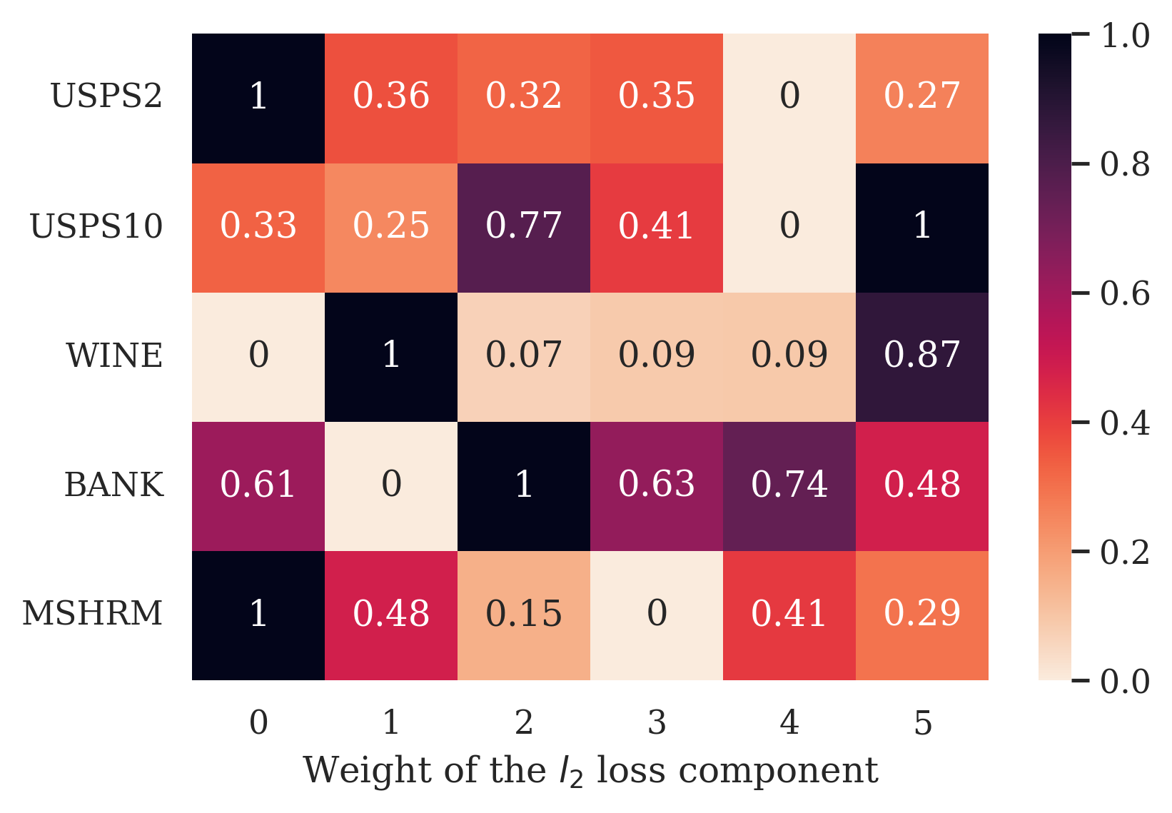
For the other 4 datasets, we carried out a narrower grid search. We found that the best-performing loss had the same weights for most components as reported in Equation 27. Only the component weight changed, as shown in Figure 8.
4.5 Empirical evaluation of the proposed conformal loss function
For the most direct comparison between our conformal loss function (Section 3.2), Aggregated Conformal Prediction (ACP), and Inductive Conformal Prediction (ICP), we use the same feedforward neural network (NN) model in all tests: as a standalone Deep Learning (DL) model and as the underlying model for ACP and ICP, since any point predictor may be used (Section 2). The ACP p-value aggregation procedure and ICP non-conformity-measure are given in Equations 7 and 3 respectively. Readers are referred to Section 2.1 for a detailed background on CP.
Ten iterations were evaluated in all 3 scenarios. For DL and ICP, each iteration represents an independent run, and the average is reported; For ACP, each run had a different number of ensemble models from . Each NN model was trained with our novel conformal loss function after parameter optimisation (Section 4). The models were evaluated with metrics suited to Conformal Prediction, as described in Section 4.3. We start with a detailed overview of the binary classification results and then explore how the increase of classes and training samples affected the model performance. Overall, our analysis had a stronger focus on calibration adherence at lower significance levels , since low error rates are especially relevant to most prediction tasks with confidence requirements.
To give a comprehensive results analysis, we first evaluate the MNIST dataset for the binary and multi-class tasks in great detail (Section 4.5.1), after which we highlight similarities and differences for the additional 4 datasets (Section 4.5.2).
4.5.1 MNIST evaluation
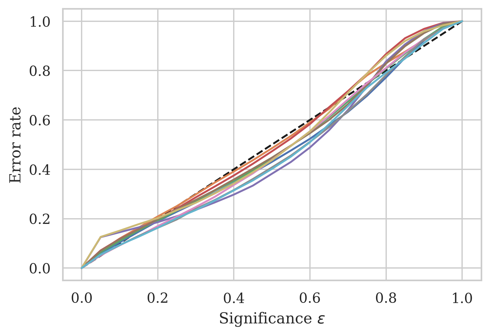
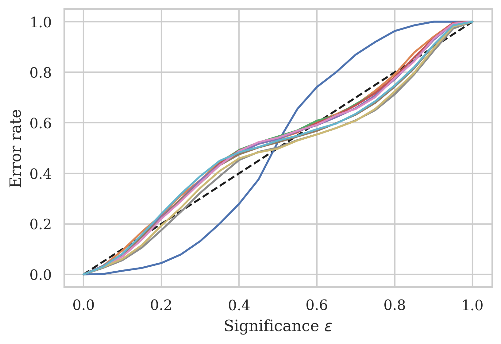
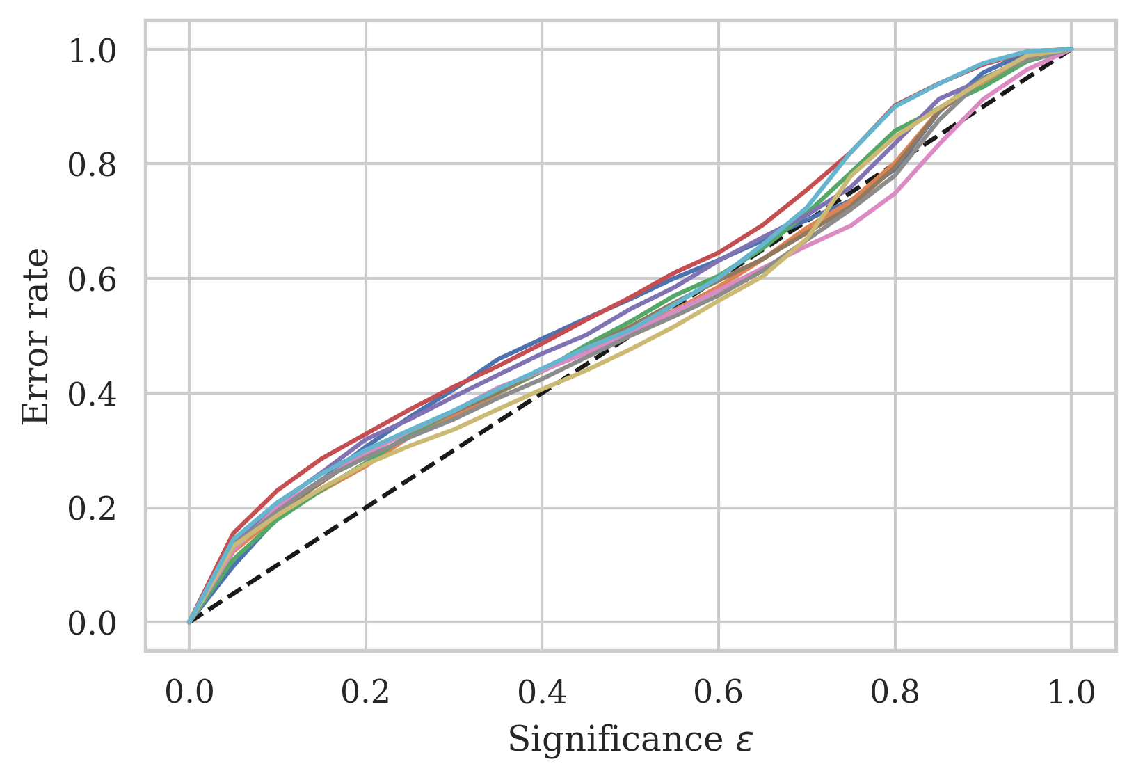
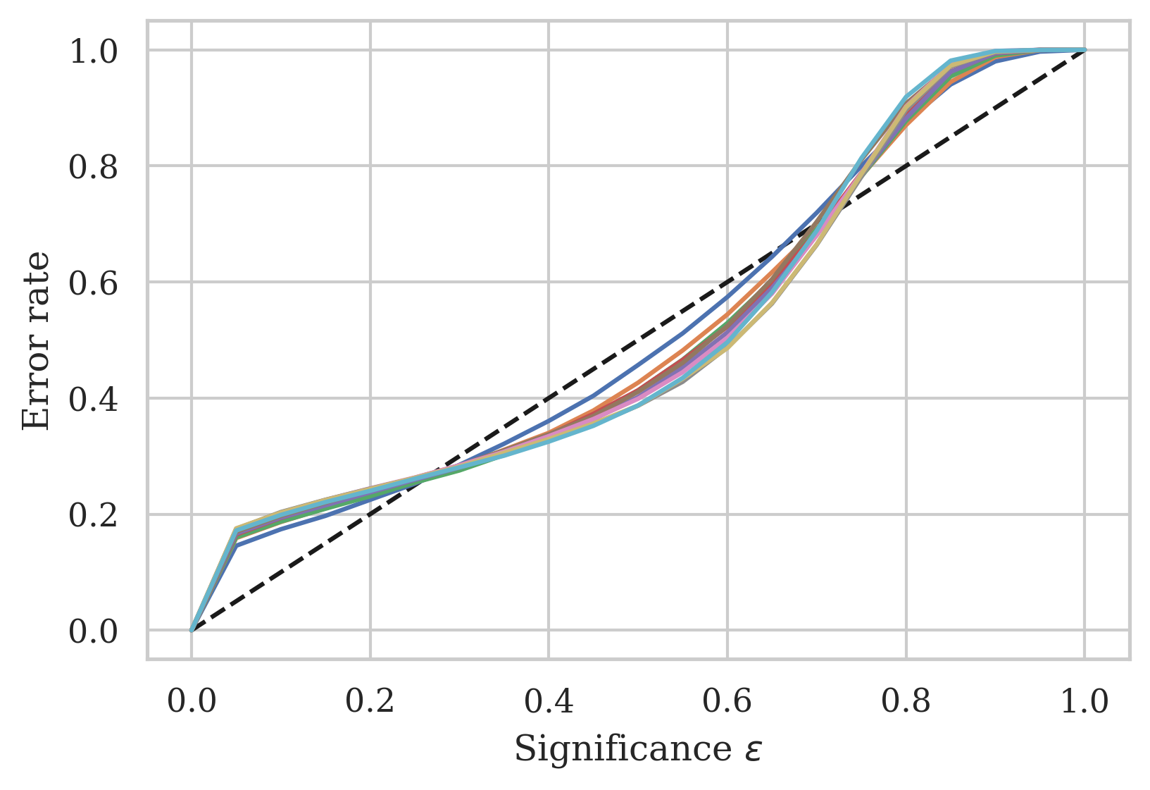
Figure 9 confirms that the error rate of the CP approximation with our proposed NN loss function roughly followed the calibration curve (dashed line) for binary classification on the MNIST2 dataset. Unlike ACP, which with has a distinctive S-shaped curve (as previously noted in linusson2017calibration ), our proposal seemed to conform much more closely to the ideal validity curve at any given point. While NN error rates were conservative at low significance (), the gap was overall smaller than ACP with .
Hence, the results confirm that our conformal loss achieved approximate validity without computing intermediate non-conformity measures. The calibration curve deviations and their concrete effects will be examined in more detail when we evaluate the calibration/efficiency trade-off later in this section.
Approximate validity
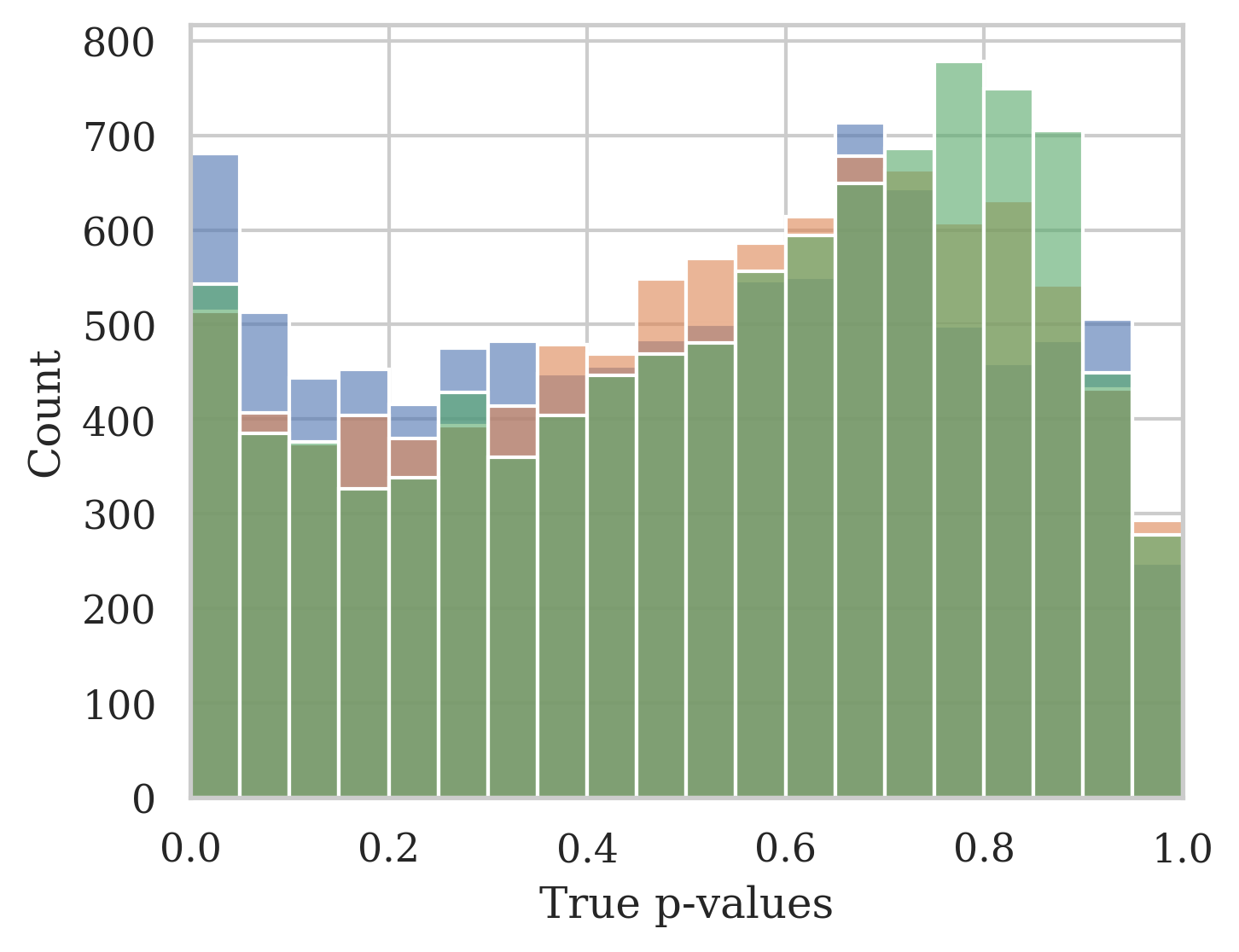
To preserve validity, p-values of the true class should follow the uniform distribution . On the other hand, false-class p-values should be as close to 0 as possible to maximise predictive efficiency (Section 3.1). An NN trained with our conformal loss function tended to a bi-modal distribution of true-class p-values, dipping around 0.5 (Figure 10), which may be a side-effect of the Huber loss component. Inversely, ACP tended to a unimodal distribution, peaking at 0.5 (Figure 10(b)). However, we note that was also bimodal and distinctly similar to the NN trends.
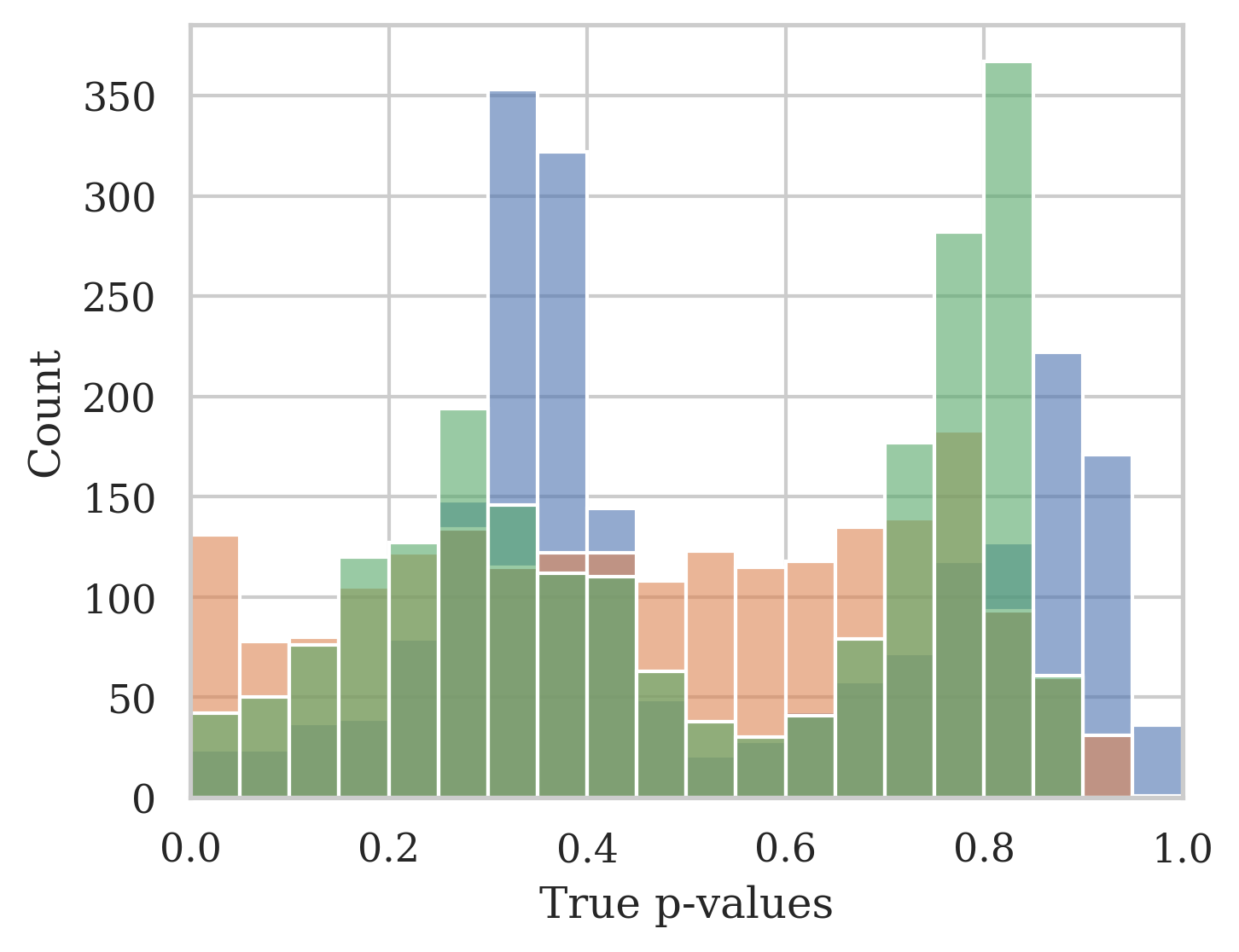
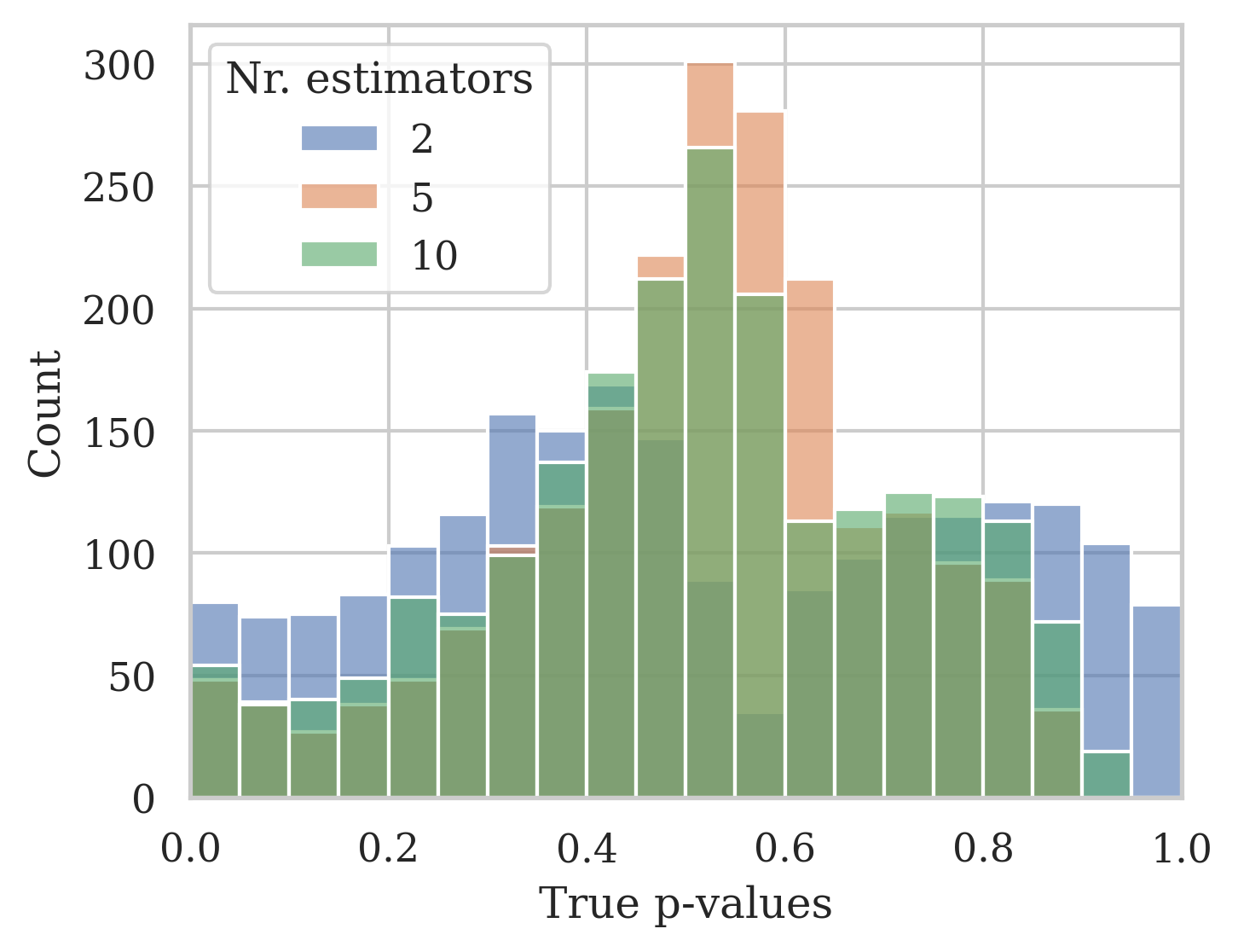
These findings are directly related to the calibration lines and explain previous observations in Figure 1: NN with true p-values concentrated towards the extremes tended to be slightly conservative at lower () and higher () significance levels. In contrast, ACP had a distinctive S-shape and was significantly conservative until , after which the calibration curve crossed the diagonal and became invalid.
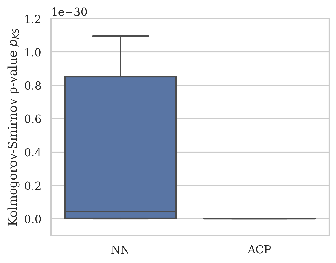
Neither method passed the Kolmogorov-Smirnov test of uniformity zhang2010fast , since all p-values were lower than our significance level (Figure 10(c)). However, NN were distributed across a larger range than ACP ( has an inverse relationship with ), which shows that our method has the potential to achieve stronger approximate validity with future loss function optimisations.
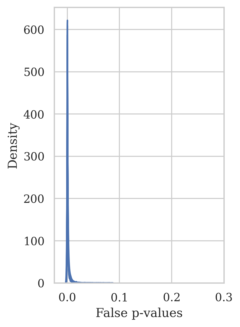
Predictive efficiency
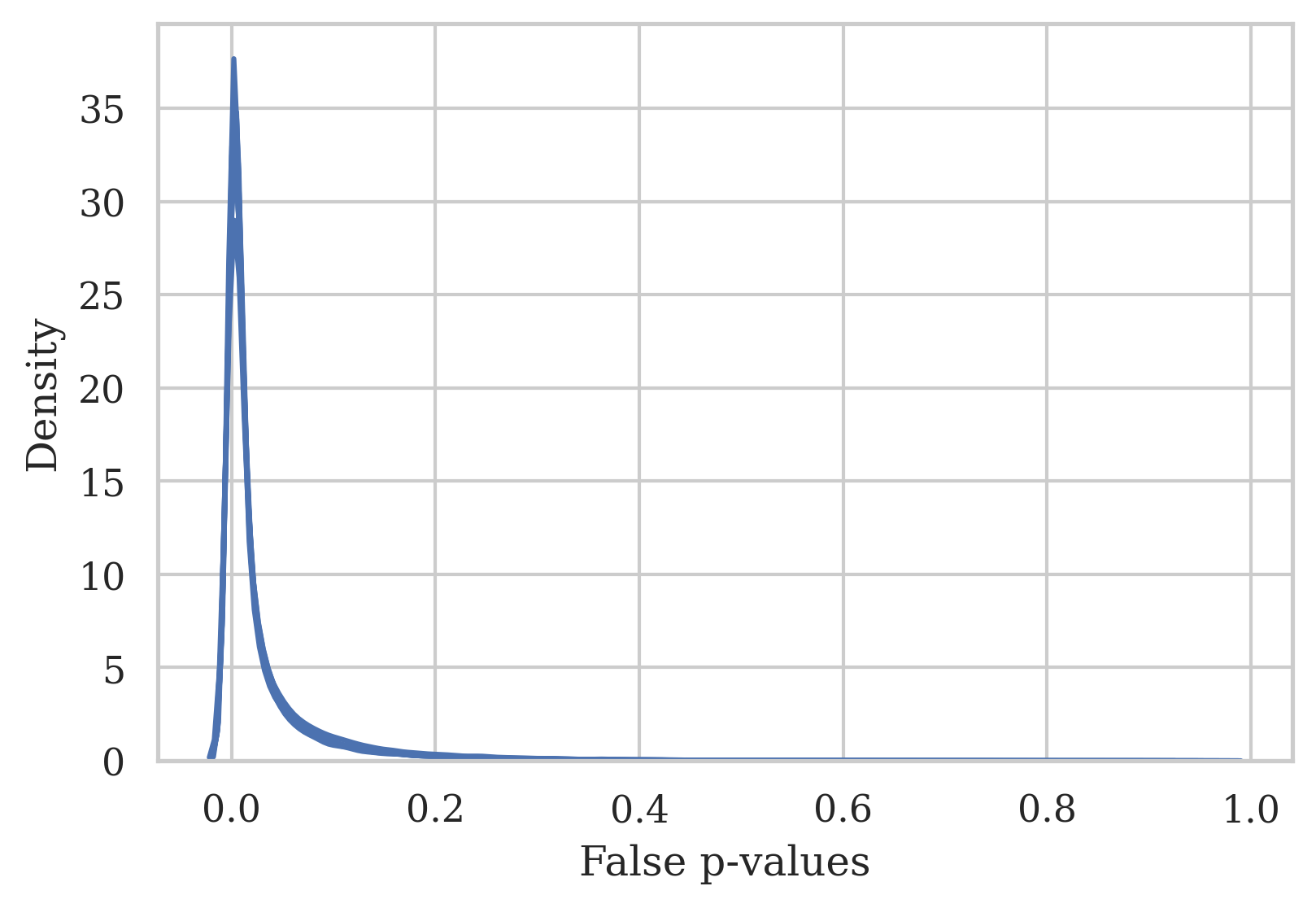
Figure 11 shows that the false-class p-values were centred around 0 for both methods. Surprisingly, increasing the number of models for ACP did not seem to improve predictive efficiency in this case, as all distribution curves were almost indistinguishably overlapped (Figure 11(b)). While NN false p-values had slightly more spread up to 0.0005 (Figure 11(a)), the values were still orders of magnitude under the minimum threshold considered in this study, and therefore did not affect the prediction set sizes.

Calibration vs predictive efficiency trade-off
After examining the p-value distributions, we may more meaningfully compare our proposed one-step conformal p-value approximation to traditional ACP on a more holistic level. We evaluated the predictive efficiency gains in the context of the distance of the error line to the calibration curve.
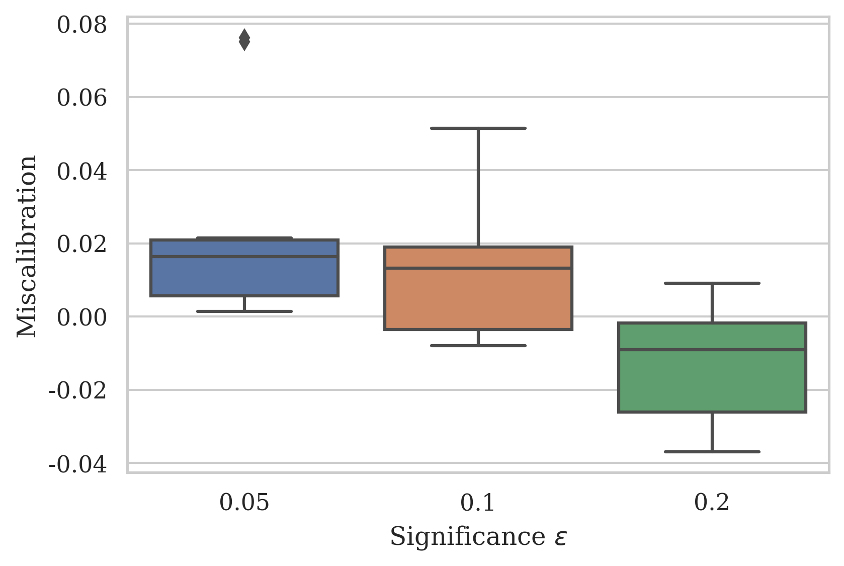
As discussed in Section 2, ACP improves predictive efficiency by increasing set sizes towards the optimal as the number of ensemble models grows, with the side-effect of a weaker validity approximation (Figure 12(b)). Although the effects were relatively minor for small significance levels (), the positive efficiency and negative calibration trends became much more pronounced as grew.
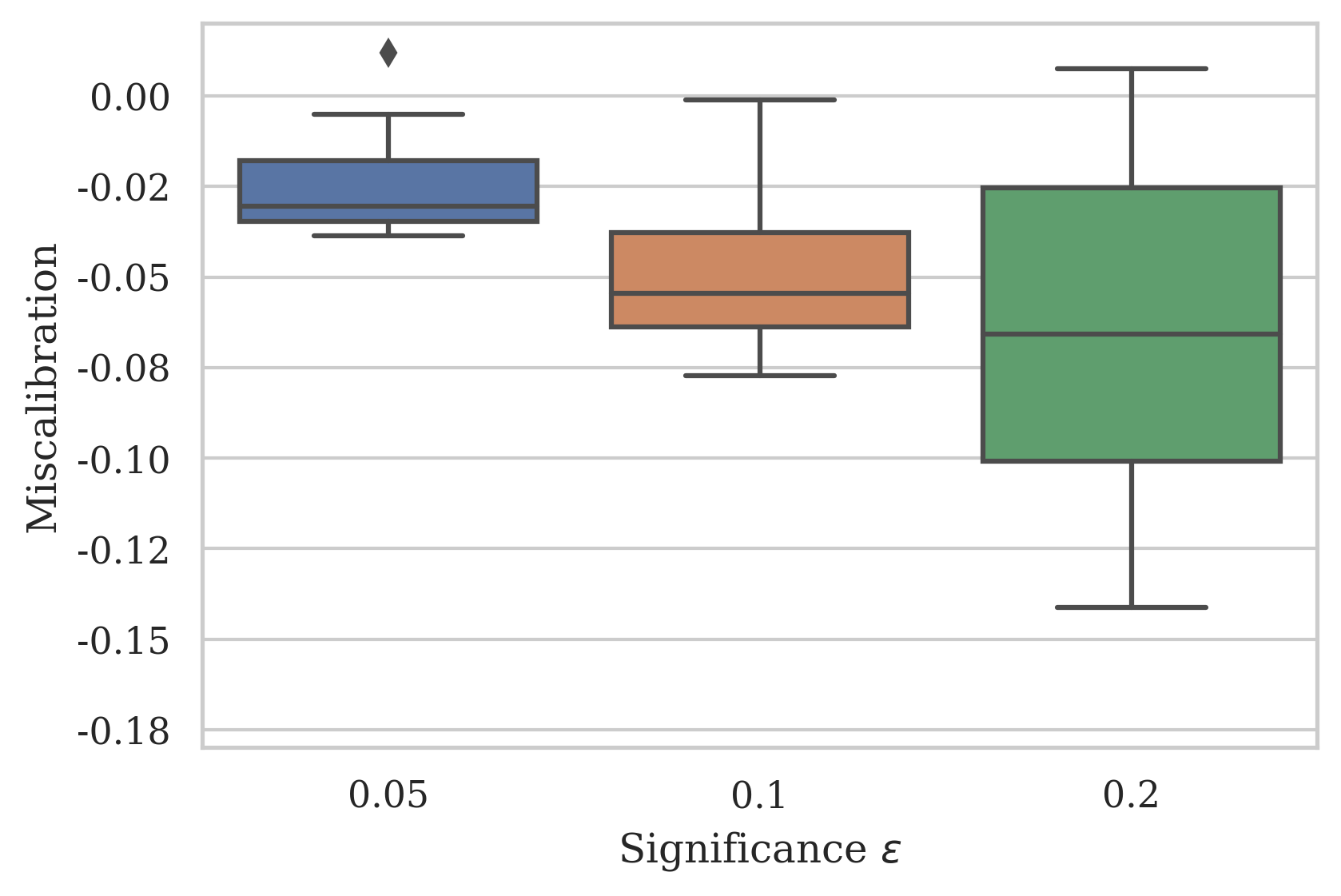
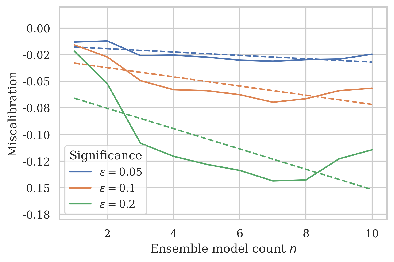
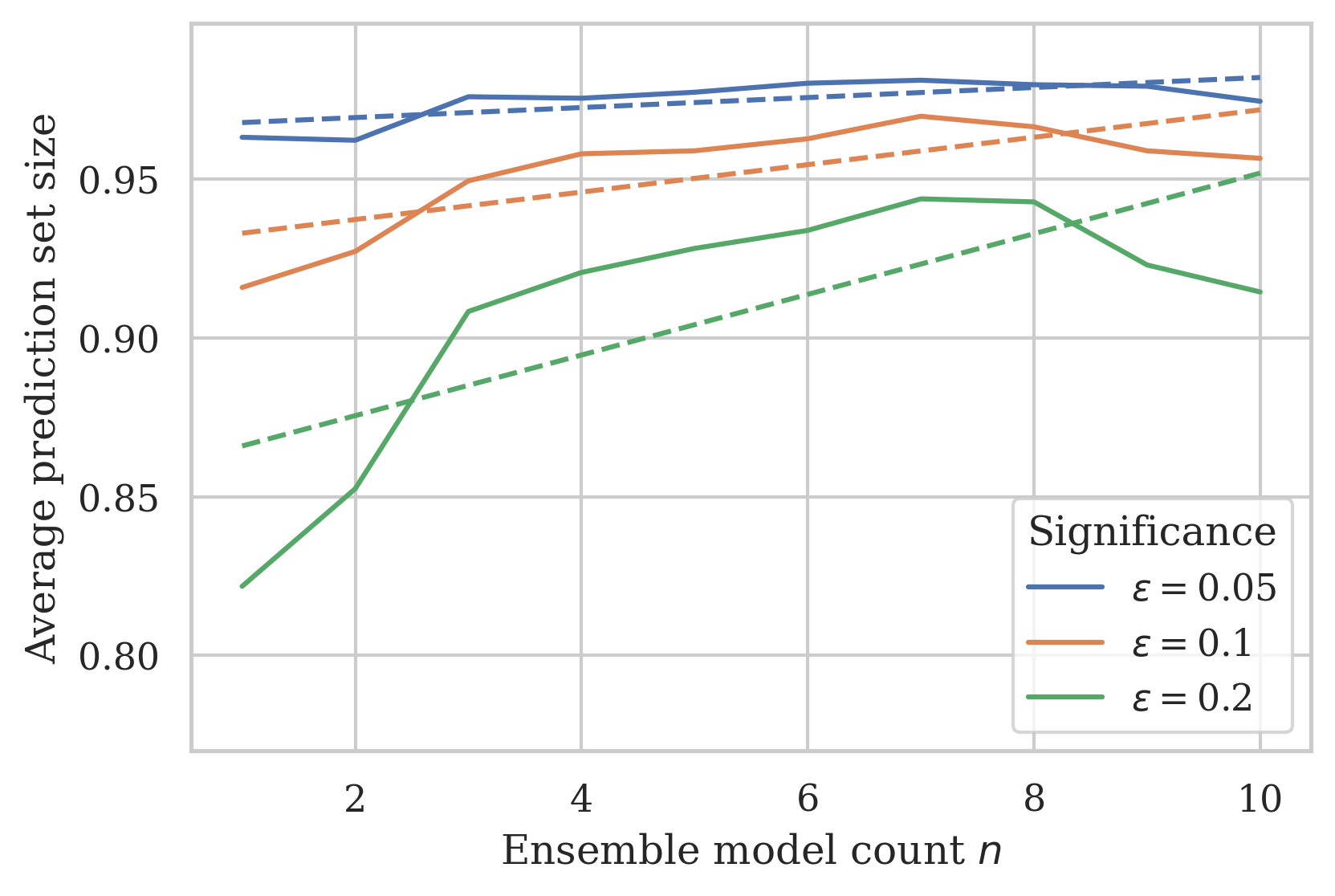
Promisingly, the average calibration of our conformal loss NN with was competitive with the equivalent ACP trend line across all , and the range improved the distance towards 0 in some iterations (Figure 12(a)). At , NN again improved on ACP, with the mean equivalent to and some iterations reaching nearly perfect calibration (calibration distance 0). The largest improvement on average was achieved at , which on average significantly outperformed the ACP equivalent for .
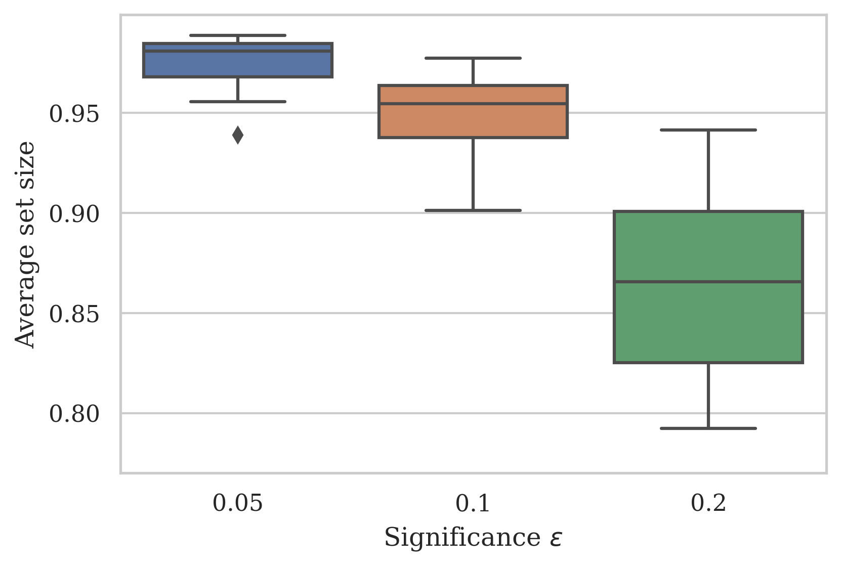
In predictive efficiency, we may confirm again that our proposed loss function is competitive with ACP without major deficits. CP’s optimal prediction set size is 1, and Figures 12(c) and 12(d) highlight that both models performed well, especially at low significance levels (NN=0.97 and ACP=0.96–0.97 for . As expected, ACP average set sizes improved as the number of ensemble models increased. Similarly to the calibration distance, the trend slopes were shallower at low significance levels, and taking the calibration trade-off by increasing had a higher value of return at higher significance levels. Similarly, the NN model’s predictive efficiency also showed larger ranges and variability as significance levels increased. This supports our previous assessment that the marginally increased p-values compared to ACP do not affect predictive efficiency.
Standard CP performance metrics in Table 4 confirm our observations so far. Both NN and ACP were conservative for low significance levels, although ACP achieved error scores closer to the expected maximum. Additionally, the minor increase in NN false p-values was negligible even at , all significance levels show 0% multi-sets and a high single-set rate. In combination with lower error rates, we conclude that our proposed conformal loss function successfully trains a simple NN model to confidently assign only the correct class to the vast majority of samples, without first calculating an additional non-conformity measure (Section 3.2).
| NN | ACP, | ACP, | ICP | |||||||||
|---|---|---|---|---|---|---|---|---|---|---|---|---|
| 0.05 | 0.1 | 0.2 | 0.05 | 0.1 | 0.2 | 0.05 | 0.1 | 0.2 | 0.05 | 0.1 | 0.2 | |
| Error | 2.61 | 5.31 | 13.58 | 4.49 | 9.50 | 20.38 | 1.89 | 5.77 | 20.76 | 3.56 | 8.28 | 18.37 |
| Empty | 2.59 | 5.31 | 13.58 | 4.44 | 9.50 | 20.38 | 1.89 | 5.77 | 20.76 | 3.42 | 8.23 | 18.36 |
| Single | 97.40 | 94.69 | 86.42 | 95.56 | 90.50 | 79.62 | 98.11 | 94.23 | 79.24 | 96.58 | 91.77 | 81.64 |
| Multi | 0.00 | 0.00 | 0.00 | 0.00 | 0.00 | 0.00 | 0.00 | 0.00 | 0.00 | 0.00 | 0.00 | 0.00 |
Computational efficiency
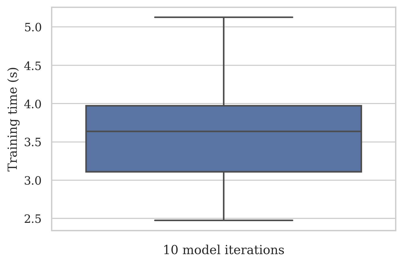
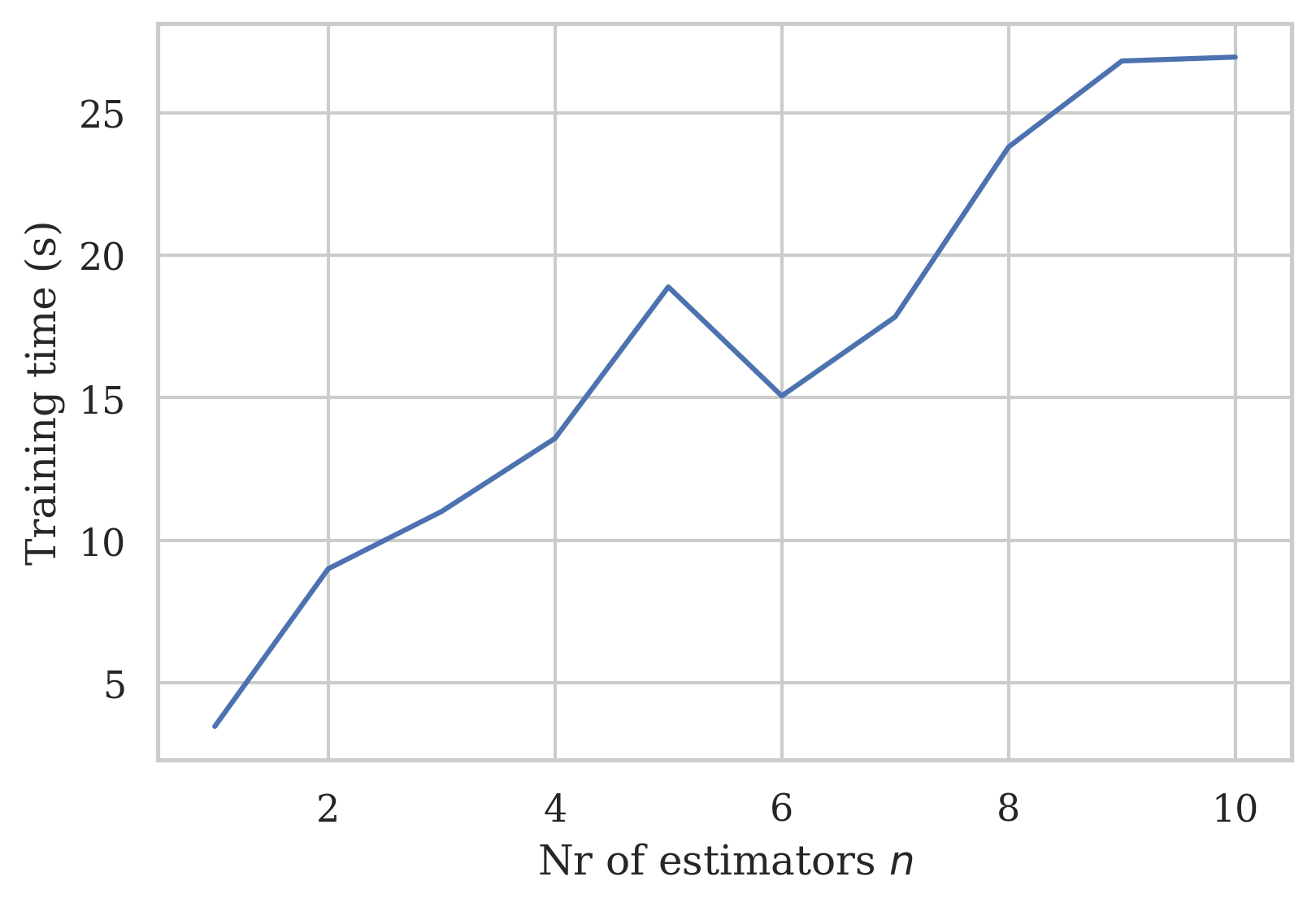
After confirming that our proposed conformal loss function successfully maintains approximate validity and predictive efficiency on par with ACP for , we evaluate the two methods’ computational efficiency in Figure 13. This is where our model has two advantages: It skips the intermediate non-conformity measure calculation and requires training only one model. In contrast, ACP’s training time increases linearly as the number of ensemble models increases. As a consequence, all test iterations of our proposed model significantly outperformed ACP with (3.5 seconds on average compared to up to over 25 seconds). Depending on and parallel computing capabilities, the training time gap may be narrowed, but ACP would nonetheless require significantly more computational power to train its ensemble models.
Increasing the number of classes and samples
Figure 14 presents our proposed method’s performance on the MNIST10 dataset. This involves differentiating between 10 classes (digits 0–9) instead of two (0, 1), and a consequent increase of training samples from around 13,000 to 60,000 (see Table 1).
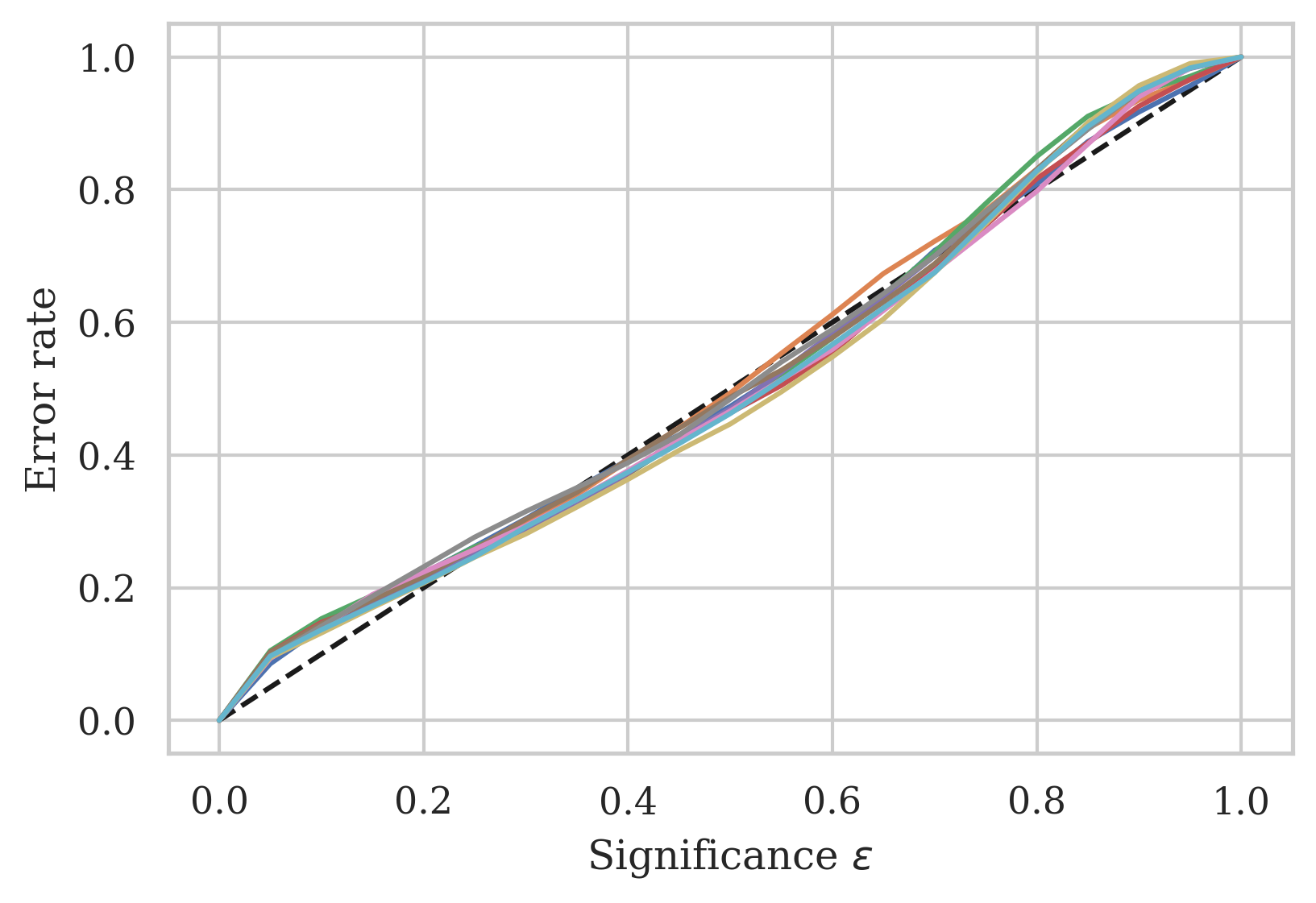
The calibration curves became visibly closer to the diagonal (exact validity), smooth, and consistent between model iterations compared to binary classification (Figure 9(a)). Additionally, all ten models achieve close to exact validity for . The smoothness of the calibration curves was a reflection of the true-class p-value distribution, which more closely followed the uniform distribution .
4.5.2 Evaluation of all datasets
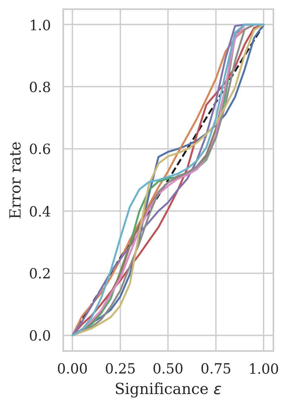
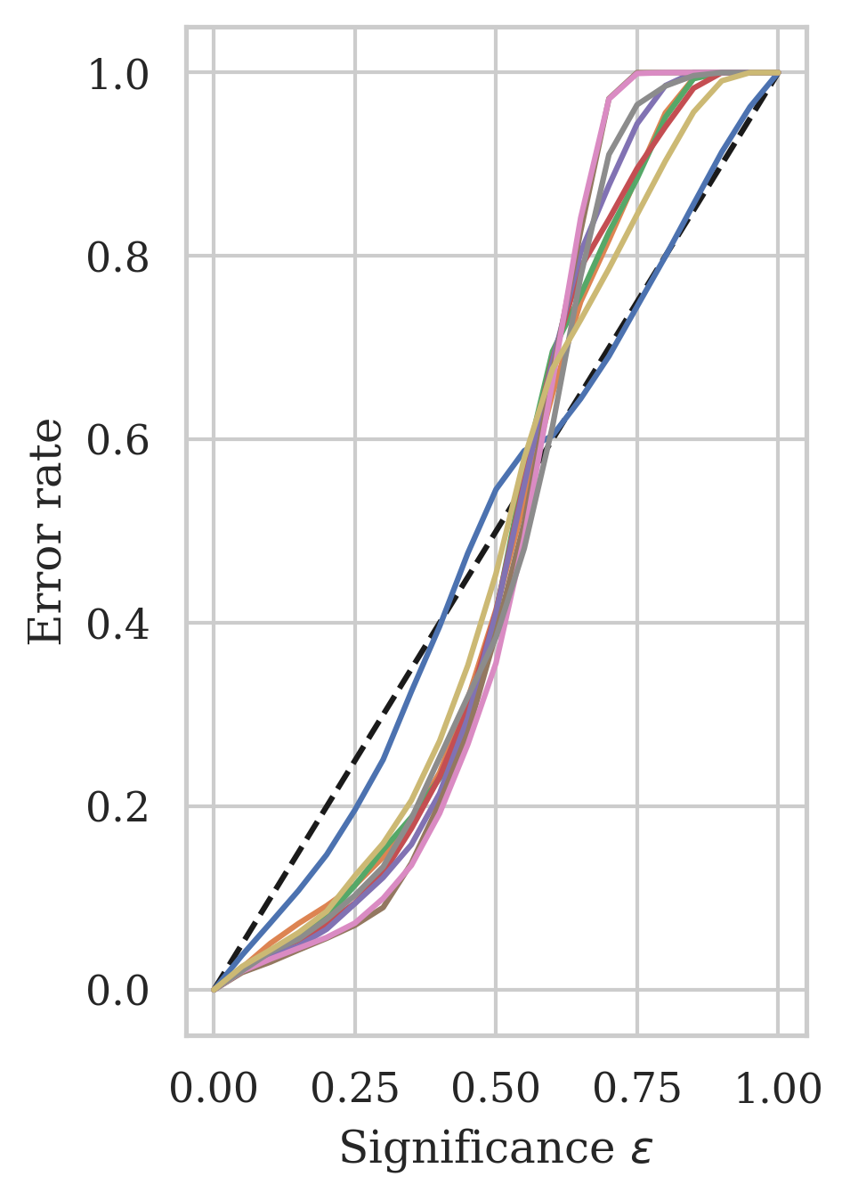
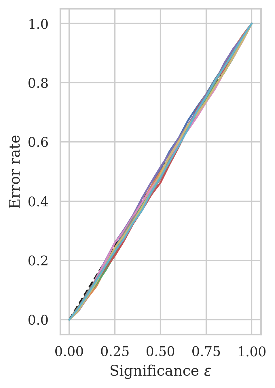
Figure 15 shows that the error lines for the remaining datasets (USPS2, USPS10, BANK, WINE, MSHRM) approximately follow the diagonal. This means that our DL approximation is successful, and our conformal loss function can be transferred from the MNIST2 and MNIST10 datasets onto new and unseen datasets with similar performance. The best results are achieved on the USPS10 (multi-class) and MSHRM (binary) datasets, perhaps because of the relatively large sample sizes. However, in comparison, the BANK dataset also has more than 40,000 samples and did not perform as well, so the underlying cause merits further investigation.

A detailed breakdown of our results and ACP results for comparison is given in Table 5. Interestingly, NN approximation multi-set prediction rates tend to be significantly lower than ACP rates (e.g., USPS10 with ACP multi-rate compared to NN multi-rate ). An extreme case may be observed for the WINE dataset (binary), where all predictions are multi-set predictions containing both labels. Furthermore, this trend is accompanied by NN average set sizes being closer to one (optimal prediction) in most cases. This is particularly noticeable for the USPS10 dataset (ACP average ). Furthermore, the fuzziness of the NN approximation tends to be slightly improved over ACP results. In other words, the p-values, apart from the largest p-value, tend to be close to 0, which explains the overall low multi-set rates and average set sizes.
Finally, as expected, the training time is much lower for the NN approach compared to ACP, since only one model must be trained at a time.
| Model | Metric | MNIST2 | MNIST10 | USPS2 | USPS10 | BANK | WINE | MSHRM |
|---|---|---|---|---|---|---|---|---|
| NN | Error | 5.31% | 11.43% | 12.15% | 19.71% | 19.39% | 13.98% | 14.28% |
| Empty | 5.31% | 5.34% | 10.59% | 12.12% | 16.35% | 9.85% | 13.75% | |
| Single | 94.69% | 48.64% | 78.22% | 63.65% | 83.65% | 89.85% | 86.14% | |
| Multi | 0.00% | 46.02% | 2.70% | 24.23% | 0.00% | 0.30% | 0.11% | |
| Avg. | 0.95 | 1.60 | 0.96 | 1.31 | 0.84 | 0.90 | 0.86 | |
| Miscal. | 1.11 | 0.73 | 0.90 | 1.01 | 1.26 | 0.80 | 0.48 | |
| Fuzz. | 0.00 | 0.26 | 0.01 | 0.08 | 0.00 | 0.00 | 0.00 | |
| Time | 3.64s | 8.29s | 1.48s | 1.18s | 1.87s | 0.78s | 2.53s | |
| ACP-2 | Error | 7.28% | 5.20% | 2.09% | 3.64% | 9.23% | 9.60% | 8.19% |
| Empty | 7.28% | 0.00% | 1.61% | 0.00% | 0.00% | 0.00% | 0.00% | |
| Single | 92.72% | 69.30% | 98.39% | 28.40% | 98.10% | 82.56% | 98.45% | |
| Multi | 0.00% | 30.70% | 0.00% | 71.60% | 1.90% | 17.44% | 1.55% | |
| Avg. | 0.93 | 1.89 | 0.98 | 4.68 | 1.02 | 1.17 | 1.02 | |
| Miscal. | 0.43 | 0.66 | 2.29 | 0.87 | 0.37 | 0.59 | 0.39 | |
| Fuzz. | 0.00 | 0.30 | 0.00 | 0.90 | 0.02 | 0.05 | 0.02 | |
| Time | 9.00s | 16.39s | 4.98s | 4.57s | 6.36s | 4.27s | 6.19s | |
| ACP-5 | Error | 4.11% | 4.32% | 1.28% | 4.63% | 8.05% | 0.00% | 7.17% |
| Empty | 4.11% | 0.00% | 0.00% | 0.00% | 0.00% | 0.00% | 0.00% | |
| Single | 95.89% | 68.97% | 88.44% | 35.28% | 96.28% | 0.00% | 97.45% | |
| Multi | 0.00% | 31.03% | 11.56% | 64.72% | 3.72% | 100.00% | 2.55% | |
| Avg. | 0.96 | 2.06 | 1.12 | 4.75 | 1.04 | 2.00 | 1.03 | |
| Miscal. | 2.15 | 0.78 | 3.44 | 0.74 | 0.93 | 3.60 | 0.56 | |
| Fuzz. | 0.00 | 0.34 | 0.04 | 0.84 | 0.02 | 0.42 | 0.02 | |
| Time | 18.90s | 43.36s | 11.28s | 11.25s | 15.30s | 11.96s | 19.51s | |
| ACP-10 | Error | 4.35% | 4.67% | 0.48% | 2.39% | 8.97% | 0.00% | 6.82% |
| Empty | 4.35% | 0.00% | 0.00% | 0.00% | 0.00% | 0.00% | 0.00% | |
| Single | 95.65% | 81.63% | 98.56% | 32.44% | 98.22% | 0.00% | 96.92% | |
| Multi | 0.00% | 18.37% | 1.44% | 67.56% | 1.78% | 100.00% | 3.08% | |
| Avg. | 0.96 | 1.53 | 1.01 | 3.93 | 1.02 | 2.00 | 1.03 | |
| Miscal. | 1.68 | 0.93 | 2.21 | 1.14 | 0.85 | 2.71 | 0.61 | |
| Fuzz. | 0.00 | 0.28 | 0.05 | 0.76 | 0.02 | 0.25 | 0.02 | |
| Time | 26.96s | 128.01s | 22.16s | 24.35s | 30.21s | 29.18s | 34.84s |
5 Discussion
We presented a comprehensive empirical evaluation of our proposal on 7 classification tasks over 5 benchmark datasets. Results across ten experiment iterations found that our conformal loss function is competitive with ACP for approximate validity and predictive efficiency. The crucial difference is that our direct approach needs only one model and therefore has significantly improved computational efficiency. The computational benefit increases proportionally as the number of ensemble models in ACP grows.
Our novel loss function minimises the difference between the model output with the expected CP output distribution (Section 3). Because the false-class p-values follow the same trend as false-class probability outputs in standard DL classification (values close to 0), our loss component is successful. Consequently, we achieve high predictive efficiency and are comparable with ACP up to ensemble models at low significance levels (Figure 12(c)). The optimal and most precise prediction for CP models is (Section 2.1), and our conformal DL models achieve on average , exactly on par with ACP () at .
In terms of true-class outputs, we achieve approximate validity on par with ACP for (Table 4), measured with the Kolmogorov-Smirnov test for uniformity zhang2010fast . ACP tends to be conservative for low significance levels and invalid for higher levels linusson2017calibration . In contrast, our proposed method has a calibration line on average closer to the expected diagonal at most individual points.
Overall, our proposed approach results in ‘less invalid’ predictors compared to ACP models with the same NN underlying algorithm on the 7 classification tasks. The results analysis and interpretation in this article may be specific to the feedforward networks that were used and merits further investigation for further model architectures. However, the loss function derived from the MNIST dataset was successfully transferred to 4 new datasets, which strongly supports the generalisability of our approach.
Our proposed loss function may be refined to train predictors closer to absolute validity by improving the uniformity measure. To maintain differentiability, we measure the deviation through distribution moments (Section 3), which are not necessarily unique to the expected distribution . Empirically, we achieve approximate uniformity and therefore approximate validity, but the distribution measure may be improved in future work. Nonetheless, approximate validity may prove useful for many real-world scenarios.
6 Conclusion and future directions
We propose a novel conformal loss function which approximates the two-step CP framework for classification with one conformal loss function. By learning to output predictions in the distribution characteristic to CP from the input data (Section 2), models trained with our loss function skip the intermediate non-conformity score, hence, reducing the inherent algorithmic complexity. The loss function is fully differentiable and compatible with any gradient descent-based Deep Learning neural network (Section 3.2). Our novel approach is most successful for small significance levels, which in practice are of high interest to guarantee low error rates. Additionally, our direct conformal p-value prediction has the potential to simplify CP optimisation with further study.
We carried out an extensive and rigorous empirical evaluation of our proposed method for 7 classification tasks on 5 benchmark datasets, with three main insights:
-
•
Our proposal is comparative to Aggregated Conformal Prediction (ACP) for low significance levels, a common CP variant that has been successful on real-world datasets with high predictive efficiency (see Section 2.1). We achieve results on par with ACP for both approximate validity and predictive efficiency when ensemble models.
-
•
Notably, our conformal loss function significantly improves ACP’s computational efficiency without compromising CP performance. We train only one model, compared to ACP ensemble models. As increases, the computational savings of our method grow proportionally.
-
•
Finally, our one-step CP approximation reduces the algorithmic complexity of the traditionally two-step CP framework. This provides a potential new avenue for CP optimisation research, which is traditionally a difficult task since the interaction between the underlying algorithm and the non-conformity measure have to be considered simultaneously (see Section 2.2).
Future work includes improving our conformal loss function to achieve guaranteed validity over approximate validity. For example, this may be achieved by improving the output uniformity metric to be more precise (Section 5). Additionally, our empirical study may be extended with a theoretical evaluation and optimisation of the loss function for gradient descent to improve model convergence.
Declarations
-
•
Funding: This research is funded by University of Brighton’s ‘Rising Stars’ research grant, and Innovate UK’s AKT2I grant ‘Machine vision segmentation for automated UK train tracking and railway maintenance’.
-
•
Conflict of interest/Competing interests: The authors declare that they have no conflict of interest.
-
•
Availability of data and materials: The 5 datasets analysed during the study are publicly available as follows: The MNIST dataset lecun1998gradient at http://yann.lecun.com/exdb/mnist/; The USPS dataset hull1994database at https://www.kaggle.com/datasets/bistaumanga/usps-dataset; And the WINE CorCer09 , BANK moro2014data , and MSHRM schlimmer1981mushroom datasets were obtained from the UCI Machine Learning Repository Dua2019 at https://archive.ics.uci.edu.
-
•
Code availability: The code is available at https://github.com/juliameister/dl-confident-loss-function.
References
- \bibcommenthead
- (1) Shafer, G., Vovk, V.: A tutorial on conformal prediction. Journal of Machine Learning Research 9(3) (2008)
- (2) Norinder, U., Boyer, S.: Conformal prediction classification of a large data set of environmental chemicals from ToxCast and Tox21 estrogen receptor assays. Chemical research in toxicology 29(6), 1003–1010 (2016)
- (3) Rechkemmer, A., Yin, M.: When confidence meets accuracy: Exploring the effects of multiple performance indicators on trust in machine learning models. In: CHI Conference on Human Factors in Computing Systems, pp. 1–14 (2022)
- (4) Zhang, T., Sun, M., Cremer, J.L., Zhang, N., Strbac, G., Kang, C.: A confidence-aware machine learning framework for dynamic security assessment. IEEE Transactions on Power Systems 36(5), 3907–3920 (2021)
- (5) Meister, J.A., Nguyen, K.A., Luo, Z.: Audio feature ranking for sound-based COVID-19 patient detection. In: Progress in Artificial Intelligence (2022). Springer
- (6) Yin, M., Wortman Vaughan, J., Wallach, H.: Understanding the effect of accuracy on trust in machine learning models. In: Proceedings of the 2019 Chi Conference on Human Factors in Computing Systems, pp. 1–12 (2019)
- (7) Vovk, V., Gammerman, A., Shafer, G.: Algorithmic Learning in a Random World. Springer, US (2005)
- (8) Riquelme-Granada, N., Nguyen, K., Luo, Z.: Coreset-based conformal prediction for large-scale learning. In: Conformal and Probabilistic Prediction and Applications, pp. 142–162 (2019). PMLR
- (9) Linusson, H., Norinder, U., Boström, H., Johansson, U., Löfström, T.: On the calibration of aggregated conformal predictors. In: Conformal and Probabilistic Prediction and Applications, pp. 154–173 (2017). PMLR
- (10) Papadopoulos, H., Vovk, V., Gammerman, A.: Conformal prediction with neural networks. In: 19th IEEE International Conference on Tools with Artificial Intelligence (ICTAI 2007), vol. 2, pp. 388–395 (2007). IEEE
- (11) LeCun, Y., Bengio, Y., Hinton, G.: Deep learning. Nature 521(7553), 436–444 (2015)
- (12) Maskara, N., Kubica, A., Jochym-O’Connor, T.: Advantages of versatile neural-network decoding for topological codes. Physical Review A 99(5), 052351 (2019)
- (13) Khatri, N., Khatri, K.K., Sharma, A.: Prediction of effluent quality in ICEAS-sequential batch reactor using feedforward artificial neural network. Water science and technology 80(2), 213–222 (2019)
- (14) Cherubin, G., Chatzikokolakis, K., Jaggi, M.: Exact optimization of conformal predictors via incremental and decremental learning. In: International Conference on Machine Learning, pp. 1836–1845 (2021). PMLR
- (15) Vovk, V.: Conditional validity of inductive conformal predictors. In: Asian Conference on Machine Learning, pp. 475–490 (2012). PMLR
- (16) Gupta, C., Kuchibhotla, A.K., Ramdas, A.: Nested conformal prediction and quantile out-of-bag ensemble methods. Pattern Recognition 127, 108496 (2022)
- (17) Johansson, U., Boström, H., Löfström, T., Linusson, H.: Regression conformal prediction with random forests. Machine learning 97(1), 155–176 (2014)
- (18) Fisch, A., Schuster, T., Jaakkola, T., Barzilay, R.: Few-shot conformal prediction with auxiliary tasks. In: International Conference on Machine Learning, pp. 3329–3339 (2021). PMLR
- (19) Löfström, T., Johansson, U., Boström, H.: Effective utilization of data in inductive conformal prediction using ensembles of neural networks. In: The 2013 International Joint Conference on Neural Networks (IJCNN), pp. 1–8 (2013). IEEE
- (20) Norinder, U., Boyer, S.: Binary classification of imbalanced datasets using conformal prediction. Journal of Molecular Graphics and Modelling 72, 256–265 (2017)
- (21) Johansson, U., Linusson, H., Löfström, T., Boström, H.: Model-agnostic nonconformity functions for conformal classification. In: 2017 International Joint Conference on Neural Networks (IJCNN), pp. 2072–2079 (2017). IEEE
- (22) Johansson, U., Boström, H., Löfström, T.: Conformal prediction using decision trees. In: 2013 IEEE 13th International Conference on Data Mining, pp. 330–339 (2013). IEEE
- (23) Vovk, V.: Transductive conformal predictors. In: IFIP International Conference on Artificial Intelligence Applications and Innovations, pp. 348–360 (2013). Springer
- (24) Angelopoulos, A.N., Bates, S., Jordan, M., Malik, J.: Uncertainty sets for image classifiers using conformal prediction. In: International Conference on Learning Representations (2020)
- (25) Krstajic, D.: Critical assessment of conformal prediction methods applied in binary classification settings. Journal of Chemical Information and Modeling 61(10), 4823–4826 (2021)
- (26) Sesia, M., Romano, Y.: Conformal prediction using conditional histograms. Advances in Neural Information Processing Systems 34, 6304–6315 (2021)
- (27) Papadopoulos, H., Vovk, V., Gammerman, A.: Regression conformal prediction with nearest neighbours. Journal of Artificial Intelligence Research 40, 815–840 (2011)
- (28) Linusson, H.: Nonconformity measures and ensemble strategies: An analysis of conformal predictor efficiency and validity. PhD thesis, Department of Computer and Systems Sciences, Stockholm University (2021)
- (29) Eklund, M., Norinder, U., Boyer, S., Carlsson, L.: The application of conformal prediction to the drug discovery process. Annals of Mathematics and Artificial Intelligence 74(1), 117–132 (2015)
- (30) Meister, J.A.: Conformal predictors for detecting harmful respiratory events. Master’s thesis, Royal Holloway, University of London (2020)
- (31) Nguyen, K.A., Luo, Z.: Cover your cough: Detection of respiratory events with confidence using a smartwatch. In: Conformal and Probabilistic Prediction and Applications, pp. 114–131 (2018). PMLR
- (32) Wisniewski, W., Lindsay, D., Lindsay, S.: Application of conformal prediction interval estimations to market makers’ net positions. In: Conformal and Probabilistic Prediction and Applications, pp. 285–301 (2020). PMLR
- (33) Makili, L., Vega, J., Dormido-Canto, S.: Incremental Support Vector Machines for fast reliable image recognition. Fusion Engineering and Design 88(6-8), 1170–1173 (2013)
- (34) Papadopoulos, H., Gammerman, A., Vovk, V.: Reliable diagnosis of acute abdominal pain with conformal prediction. Engineering Intelligent Systems 17(2), 127 (2009)
- (35) Vovk, V.: Cross-conformal predictors. Annals of Mathematics and Artificial Intelligence 74(1), 9–28 (2015)
- (36) Carlsson, L., Eklund, M., Norinder, U.: Aggregated conformal prediction. In: IFIP International Conference on Artificial Intelligence Applications and Innovations, pp. 231–240 (2014). Springer
- (37) Wilm, A., Norinder, U., Agea, M.I., de Bruyn Kops, C., Stork, C., Kühnl, J., Kirchmair, J.: Skin Doctor Cp: conformal prediction of the skin sensitization potential of small organic molecules. Chemical Research in Toxicology 34(2), 330–344 (2020)
- (38) Solari, A., Djordjilović, V.: Multi split conformal prediction. Statistics & Probability Letters 184, 109395 (2022)
- (39) Toccaceli, P., Gammerman, A.: Combination of inductive mondrian conformal predictors. Machine Learning 108(3), 489–510 (2019)
- (40) Balasubramanian, V.N., Chakraborty, S., Panchanathan, S.: Conformal predictions for information fusion. Annals of Mathematics and Artificial Intelligence 74(1), 45–65 (2015)
- (41) Abad, J., Bhatt, U., Weller, A., Cherubin, G.: Approximating full conformal prediction at scale via influence functions. arXiv preprint arXiv:2202.01315 (2022)
- (42) Ghalambaz, M., Noghrehabadi, A., Behrang, M., Assareh, E., Ghanbarzadeh, A., Hedayat, N.: A hybrid neural network and gravitational search algorithm (HNNGSA) method to solve well known Wessinger’s equation. International Journal of Mechanical and Mechatronics Engineering 5(1), 147–151 (2011)
- (43) Olivé, D.M., Huynh, D.Q., Reynolds, M., Dougiamas, M., Wiese, D.: A supervised learning framework for learning management systems. In: Proceedings of the First International Conference on Data Science, E-Learning and Information Systems, pp. 1–8 (2018)
- (44) Lillicrap, T.P., Santoro, A., Marris, L., Akerman, C.J., Hinton, G.: Backpropagation and the brain. Nature Reviews Neuroscience 21(6), 335–346 (2020)
- (45) Makansi, O., Ilg, E., Cicek, O., Brox, T.: Overcoming limitations of mixture density networks: A sampling and fitting framework for multimodal future prediction. In: Proceedings of the IEEE/CVF Conference on Computer Vision and Pattern Recognition, pp. 7144–7153 (2019)
- (46) Li, C., Lee, G.H.: Generating multiple hypotheses for 3d human pose estimation with mixture density network. In: Proceedings of the IEEE/CVF Conference on Computer Vision and Pattern Recognition, pp. 9887–9895 (2019)
- (47) Zhang, H., Liu, Y., Yan, J., Han, S., Li, L., Long, Q.: Improved deep mixture density network for regional wind power probabilistic forecasting. IEEE Transactions on Power Systems 35(4), 2549–2560 (2020)
- (48) LeCun, Y., Bottou, L., Bengio, Y., Haffner, P.: Gradient-based learning applied to document recognition. Proceedings of the IEEE 86(11), 2278–2324 (1998). https://doi.org/10.1109/5.726791
- (49) Kandel, I., Castelli, M.: The effect of batch size on the generalizability of the convolutional neural networks on a histopathology dataset. ICT express 6(4), 312–315 (2020)
- (50) Hao, Y., Orlitsky, A.: Doubly-competitive distribution estimation. In: International Conference on Machine Learning, pp. 2614–2623 (2019). PMLR
- (51) Ho, Y., Wookey, S.: The real-world-weight cross-entropy loss function: Modeling the costs of mislabeling. IEEE Access 8, 4806–4813 (2019)
- (52) Jaki, T., Kim, M., Lamont, A., George, M., Chang, C., Feaster, D., Van Horn, M.L.: The effects of sample size on the estimation of regression mixture models. Educational and Psychological Measurement 79(2), 358–384 (2019)
- (53) Malz, A., Marshall, P., DeRose, J., Graham, M., Schmidt, S., Wechsler, R., Collaboration, L.D.E.S., et al.: Approximating photo-z PDFs for large surveys. The Astronomical Journal 156(1), 35 (2018)
- (54) Batu, T., Canonne, C.L.: Generalized uniformity testing. In: 2017 IEEE 58th Annual Symposium on Foundations of Computer Science (FOCS), pp. 880–889 (2017). IEEE
- (55) Meyer, G.P.: An alternative probabilistic interpretation of the Huber loss. In: Proceedings of the IEEE/CVF Conference on Computer Vision and Pattern Recognition, pp. 5261–5269 (2021)
- (56) Hull, J.J.: A database for handwritten text recognition research. IEEE Transactions on pattern analysis and machine intelligence 16(5), 550–554 (1994)
- (57) Cortez, P., Cerdeira, A., Almeida, F., Matos, T., Reis, J.: Modeling wine preferences by data mining from physicochemical properties. Decision Support Systems 47(4), 547–553 (1998)
- (58) Moro, S., Cortez, P., Rita, P.: A data-driven approach to predict the success of bank telemarketing. Decision Support Systems 62, 22–31 (2014)
- (59) Schlimmer, J.: Mushroom records drawn from the Audubon Society Field Guide to North American mushrooms. GH Lincoff (Pres), New York (1981)
- (60) Ashby, A.E., Meister, J.A., Nguyen, K.A., Luo, Z., Gentzke, W.: Cough-based COVID-19 detection with audio quality clustering and confidence measure based learning. In: Conformal and Probabilistic Prediction with Applications (2022). PMLR
- (61) Zhang, G., Wang, X., Liang, Y.-C., Liu, J.: Fast and robust spectrum sensing via Kolmogorov-Smirnov test. IEEE Transactions on Communications 58(12), 3410–3416 (2010)
- (62) Vovk, V., Fedorova, V., Nouretdinov, I., Gammerman, A.: Criteria of efficiency for conformal prediction. In: Symposium on Conformal and Probabilistic Prediction with Applications, pp. 23–39 (2016). Springer
- (63) de Chazal, P., Tapson, J., van Schaik, A.: A comparison of extreme learning machines and back-propagation trained feed-forward networks processing the MNIST database. In: 2015 IEEE International Conference on Acoustics, Speech and Signal Processing (ICASSP), pp. 2165–2168 (2015). https://doi.org/10.1109/ICASSP.2015.7178354
- (64) Lejeune, E.: Mechanical MNIST: A benchmark dataset for mechanical metamodels. Extreme Mechanics Letters 36, 100659 (2020)
- (65) Gabella, M.: Topology of learning in feedforward neural networks. IEEE Transactions on Neural Networks and Learning Systems 32(8), 3588–3592 (2020)
- (66) Kayed, M., Anter, A., Mohamed, H.: Classification of garments from fashion MNIST dataset using CNN LeNet-5 architecture. In: 2020 International Conference on Innovative Trends in Communication and Computer Engineering (ITCE), pp. 238–243 (2020). IEEE
- (67) Kadam, S.S., Adamuthe, A.C., Patil, A.B.: CNN model for image classification on MNIST and fashion-MNIST dataset. Journal of scientific research 64(2), 374–384 (2020)
- (68) Garg, A., Gupta, D., Saxena, S., Sahadev, P.P.: Validation of random dataset using an efficient CNN model trained on MNIST handwritten dataset. In: 2019 6th International Conference on Signal Processing and Integrated Networks (SPIN), pp. 602–606 (2019). IEEE
- (69) Dua, D., Graff, C.: UCI Machine Learning Repository (2017). http://archive.ics.uci.edu/ml