Dimension of Activity in Random Neural Networks

Abstract

Neural networks are high-dimensional nonlinear dynamical systems that process information through the coordinated activity of many connected units. Understanding how biological and machine-learning networks function and learn requires knowledge of the structure of this coordinated activity, information contained, for example, in cross covariances between units. Self-consistent dynamical mean field theory (DMFT) has elucidated several features of random neural networks—in particular, that they can generate chaotic activity—however, a calculation of cross covariances using this approach has not been provided. Here, we calculate cross covariances self-consistently via a two-site cavity DMFT. We use this theory to probe spatiotemporal features of activity coordination in a classic random-network model with independent and identically distributed (i.i.d.) couplings, showing an extensive but fractionally low effective dimension of activity and a long population-level timescale. Our formulae apply to a wide range of single-unit dynamics and generalize to non-i.i.d. couplings. As an example of the latter, we analyze the case of partially symmetric couplings.

Neural circuits drive behavior, sensation, and cognition through the coordinated activity of many synaptically coupled neurons. Similarly, artificial neural networks solve tasks through distributed computations among neuronlike units with trained couplings. Understanding the structure of collective activity in such high-dimensional dynamical systems is a key problem in neuroscience and machine learning, made complicated by nonlinear units and heterogeneous couplings.

In addressing this problem, studying networks with random couplings has been fruitful Sompolinsky et al. (1988); Stern et al. (2014); Bahri et al. (2020); Poole et al. (2016); Huang (2018); Wardak and Gong (2022). Gradient descent dynamics often depend sensitively on the random initial couplings Le et al. (2015); Schoenholz et al. (2016); Martens et al. (2021); Roberts et al. (2021). Random couplings can provide a substrate for computation (see reservoir computing, Jaeger and Haas (2004); Maass et al. (2007); Rivkind and Barak (2017); Susman et al. (2021)) and are a parsimonious model of background connectivity upon which structure can be introduced Mastrogiuseppe and Ostojic (2018). In certain cases, trained networks learn low-rank additions to random connectivity Schuessler et al. (2020); Martin and Mahoney (2021). Finally, chaotic random networks model asynchronous cortical dynamics observed in-vivo Arieli et al. (1996). More broadly, high-dimensional nonlinear dynamical systems with quenched disorder are important models in physics and ecology Sompolinsky et al. (1988); Flyvbjerg et al. (1993); Ciuchi et al. (1996); Aoki et al. (2014); Kadmon and Sompolinsky (2015); Aljadeff et al. (2015); Chen et al. (2018); Mastrogiuseppe and Ostojic (2018); Roy et al. (2019); Mignacco et al. (2020); Keup et al. (2021); van Meegen et al. (2021); Krishnamurthy et al. (2022); De Giuli and Scalliet (2022).

Such disordered dynamical systems are commonly studied using dynamical mean-field theory (DMFT), which reduces the dynamics to a single-site problem, allowing for self-consistent calculation of single-unit temporal statistics. However, key properties of the structure of collective activity are not visible in single units, but only in their correlations. One such property is the effective dimension, which measures the degree of coordination of network activity via the approximate number of excited collective modes Rajan et al. (2010a); Abbott et al. (2011); Huang (2018); Recanatesi et al. (2019); Engelken et al. (2020); Recanatesi et al. (2020); Hu and Sompolinsky (2022); Jazayeri and Ostojic (2021). This quantity determines a network’s ability to classify inputs Litwin-Kumar et al. (2017); Chung et al. (2018); Cohen et al. (2020); Farrell et al. (2022), learn via Hebbian plasticity Litwin-Kumar et al. (2017); Sorscher et al. (2021), generalize learned structure Litwin-Kumar et al. (2017); Sorscher et al. (2021); Cohen and Sompolinsky (2022), and generate dynamics Sussillo and Abbott (2009); Susman et al. (2021). If the effective dimension is low, the network state can be inferred from a small number of units Ganguli et al. (2012); Gao and Ganguli (2015); Gao et al. (2017); Trautmann et al. (2019).

Correlations and dimensionality have been studied in random feedforward networks Poole et al. (2016); Huang (2018), but such approaches do not generalize to recurrent dynamics due to the need to enforce self-consistency of network activity. In this Letter, we develop a two-site DMFT, based on the cavity method, for high-dimensional nonlinear dynamical systems with quenched disorder, yielding a mean-field picture of a perturbatively coupled pair of units through which joint statistics are determined. The calculation applies across a broad range of dynamics for the individual units; we assume only that single-unit order parameters can be computed through usual DMFT techniques. Although our results are thus quite general, we apply them to the network model of Sompolinsky et al. (1988) with independent and identically distributed (i.i.d.) couplings, which displays a generic transition to chaos at a critical coupling variance Kadmon and Sompolinsky (2015). We show analytically that collective activity is predominantly confined to a subspace of extensive but fractionally low dimension, previously observed only in simulations Rajan et al. (2010a); Abbott et al. (2011); Engelken et al. (2020). Our theory also reveals that collective modes have a typical timescale much longer than that of individual units. Finally, we show that our theory can capture the effect of non-i.i.d. connectivity that could arise through learning and analyze the case of partially symmetric couplings.

Model & Order Parameters: We study a network of $N$ units with pre-activations $x_{i}(t)$ and activations ${\phi_{i}(t)=\phi(x_{i}(t))}$, where $\phi(\cdot)$ is a nonlinearity. The network has quenched disorder in its couplings, ${J_{ij}\overset{\text{i.i.d.}}{\sim}\mathcal{N}(0,g^{2}/N)}$. The network dynamics are

$$T[x_{i}](t)=\eta_{i}(t),\>\>\>\eta_{i}(t)={\sum_{j}}J_{ij}\phi_{j}(t),$$ (1)

where $T[\cdot]$ is a causal functional that specifies the single-unit dynamics, allowing for generalization beyond the conventional case of Sompolinsky et al. (1988), ${T[x](t)=(1+\partial_{t})x(t)}$, to models with complex single-unit dynamics (e.g., Stern et al. (2014); Martí et al. (2018); Muscinelli et al. (2019); Beiran and Ostojic (2019); Krishnamurthy et al. (2022); Clark and Abbott (2023)). Our calculation applies to both linear and nonlinear $T[\cdot]$. In the latter case, individual pre-activations $x_{i}(t)$ may be highly non-Gaussian. We assume the system is temporally fluctuating and statistically stationary.

The classic DMFT of Sompolinsky et al. (1988) calculates the self-averaging autocovariance (two-point) function ${C^{\phi}(\tau)=\left\langle\phi_{i}(t)\phi_{i}(t+\tau)\right\rangle_{t}=\left\langle{\phi_{i}(t)\phi_{i}(t+\tau)}\right\rangle_{\bm{J}}}$ (similarly, $C^{x}(\tau)$) through an effective single-site picture. For a given realization of $\bm{J}$, to zeroth order in $1/\sqrt{N}$, the individual local fields $\eta_{i}(t)$ are Gaussian with vanishing cross covariances. The network thus decouples into $N$ noninteracting processes, $T[x](t)=\eta(t)$, where $\eta(t)$ is a Gaussian field with zero mean and autocovariance $C^{\eta}(\tau)=g^{2}C^{\phi}(\tau)$. The problem is closed by self-consistently enforcing $C^{\phi}(\tau)=\left\langle\phi(t)\phi(t+\tau)\right\rangle_{\eta}$. $C^{x}(\tau)$ may be determined subsequently. In the model of Sompolinsky et al. (1988), this single-site problem can be solved analytically due to the linearity of $T[\cdot]$ (in general, it is amenable to numerical solution; see, e.g., Stern et al. (2014); Roy et al. (2019); Mignacco et al. (2020); Krishnamurthy et al. (2022); Clark and Abbott (2023)).

In this Letter, we go beyond this single-site picture by calculating the structure of time-lagged cross covariances between units, $C_{ij}^{\phi}(\tau)=\left\langle\phi_{i}(t)\phi_{j}(t+\tau)\right\rangle_{t}\sim 1/\sqrt{N}$ (similarly, $C_{ij}^{x}(\tau)$), ${i\neq j}$. These are non-self-averaging, so we examine the self-averaging four-point function

$$\psi^{\phi}(\bm{\tau})=N\left\langle C^{\phi}_{ij}(\tau_{1})C^{\phi}_{ij}(\tau_{2})\right\rangle_{\bm{J}},\>\>\>i\neq j$$ (2)

and, analogously, $\psi^{x}(\bm{\tau})$. Our main result is that, for $N\rightarrow\infty$, $\psi^{\phi}(\bm{\tau})$ is given in Fourier space by

$$\psi^{\phi}(\bm{\omega}) =\left(M(\bm{\omega})-1\right)C^{\phi}(\omega_{1})C^{\phi}(\omega_{2}),$$ (3)

$$\text{where }M(\bm{\omega}) =\frac{1}{\left|1-2\pi g^{2}S^{\phi}(\omega_{1})S^{\phi}(\omega_{2})\right|^{2}},$$

and ${S^{\phi}(\tau)=\left\langle\delta\phi_{i}(t)/\delta\eta_{i}(t-\tau)\right\rangle_{t}=\left\langle\delta\phi_{i}(t)/\delta\eta_{i}(t-\tau)\right\rangle_{\bm{J}}}$ is the self-averaging linear response function given, as in the single-site problem, by ${S^{\phi}(\omega)=C^{\eta\phi}(\omega)/C^{\eta}(\omega)}$ where $C^{\eta\phi}(\tau)=\left\langle\eta(t)\phi(t+\tau)\right\rangle_{\eta}$ (by the Furutsu-Novikov theorem; Appendix A). For the $x$ variables, we show

$$\psi^{x}(\bm{\omega}) =|U(\bm{\omega})|^{2}C^{\phi}(\omega_{1})C^{\phi}(\omega_{2})$$

$$+U(\bm{\omega})C^{x\phi}(\omega_{1})C^{x\phi}(\omega_{2})+\text{H.c.},$$ (4)

$$\text{where}\>\>U(\bm{\omega}) =\frac{2\pi g^{2}S^{x}(\omega_{1})S^{x}(\omega_{2})}{1-2\pi g^{2}S^{\phi}(\omega_{1})S^{\phi}(\omega_{2})}.$$

Here, $C^{x\phi}(\tau)=\left\langle x(t)\phi(t+\tau)\right\rangle_{\eta}$ and $S^{x}(\tau)$ is defined in analogy with $S^{\phi}(\tau)$. Notably, once the two-point and linear response functions have been computed in the single-site picture (analytically or numerically), the four-point functions are given analytically by Eqs. 3 and Dimension of Activity in Random Neural Networks, which apply for all $T[\cdot]$. These new order parameters encode important aspects of collective activity.

Two-site cavity DMFT.—

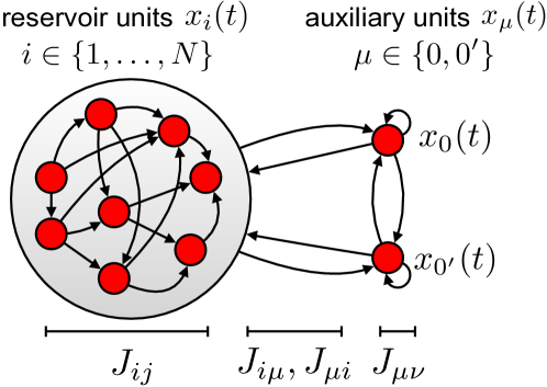
Figure 1: Overview of the two-site cavity DMFT. A cavity is created at the sites of two auxiliary units (called the cavity units) while the rest of the network, the reservoir, generates chaotic activity. The cavity units are then introduced; their effect is felt perturbatively by the reservoir. Dynamical equations for the cavity units yield a pair of perturbatively coupled mean-field equations representing a pair of units. Self-consistency conditions are constructed by noting that the cavity pair is statistically equivalent to any reservoir pair.

Our derivation is based on a two-site , dynamical Agoritsas et al. (2018); Roy et al. (2019) version of the cavity method Mézard et al. (1987); Advani et al. (2013) (Fig. 1). We add two cavity units to the network and refer to its original $N$ units as the reservoir. We use ${i,j\in\{1,\dots,N\}}$ and ${\mu,\nu\in\{0,0^{\prime}\}}$ for reservoir- and cavity-unit indices, respectively. The cavity units are bidirectionally connected to the reservoir through $J_{i\mu}$ and $J_{\mu i}$, and to one another through $J_{\mu\nu}$. In the absence of the cavity units, reservoir units follow trajectories $\phi_{i}(t)$. When the cavity units are introduced, these are perturbed by $\delta\phi_{i}(t)=\int^{t}dt^{\prime}\sum_{j}S^{\phi}_{ij}(t,t^{\prime})\sum_{\mu}J_{j\mu}\phi_{\mu}(t^{\prime}),$ $S^{\phi}_{ij}(t,t^{\prime})={\delta\phi_{i}(t)}/{\delta\eta_{j}(t^{\prime})}$. Inserting the perturbed trajectories ${\phi_{i}(t)+\delta\phi_{i}(t)}$ in Eq. 1 yields cavity-unit dynamics,

$$T[x_{\mu}](t)=\eta_{\mu}(t)+\frac{1}{\sqrt{N}}\sum_{\nu}\int^{t}dt^{\prime}F_{\mu\nu}(t,t^{\prime})\phi_{\nu}(t^{\prime}),$$ (5)

where we have defined the order-one variables

$$\eta_{\mu}(t) ={\sum_{i}}J_{\mu i}\phi_{i}(t),$$ (6)

$$F_{\mu\nu}(t,t^{\prime}) =\sqrt{N}\Bigg{[}{\sum_{ij}}J_{\mu i}J_{j\nu}S^{\phi}_{ij}(t,t^{\prime})+J_{\mu\nu}\delta(t-t^{\prime})\Bigg{]}.$$ (7)

In these definitions, the couplings and dynamic variables are mutually independent due to the cavity construction. Here, $\eta_{0}(t)$ and $\eta_{0^{\prime}}(t)$ are cavity fields, the local fields felt by the cavity units when they are not coupled to the reservoir. Due to the independence property, $\eta_{0}(t)$ and $\eta_{0^{\prime}}(t)$ are jointly temporally Gaussian, with ${\sim 1/\sqrt{N}}$ cross covariance, to first order in $1/\sqrt{N}$ .

Working in this two-site picture, we first determine an expression for $C^{\phi}_{00^{\prime}}(\omega)$. Using the joint Gaussianity of $\eta_{0}(t)$ and $\eta_{0^{\prime}}(t)$ and the decoupling of sites $0$ and $0^{\prime}$ under the time average, both valid to first order in $1/\sqrt{N}$, gives

$$C^{\phi}_{00^{\prime}}(\omega)=2\pi\Big{[}|S^{\phi}(\omega)|^{2}C^{\eta}_{00^{\prime}}(\omega)$$

$$+\frac{1}{\sqrt{N}}\left[\left(F_{00^{\prime}}(\omega)S^{\phi}(\omega)\right)^{*}+F_{0^{\prime}0}(\omega)S^{\phi}(\omega)\right]C^{\phi}(\omega)\Big{]},$$ (8)

$$\text{where }C^{\eta}_{00^{\prime}}(\omega)=\sum_{ij}J_{0i}J_{0^{\prime}j}C_{ij}^{\phi}(\omega),$$ (9)

and $F_{\mu\nu}(\tau)=\left\langle F_{\mu\nu}(t,t-\tau)\right\rangle_{t}$ (Appendix B). We square and $\bm{J}$-average Eq. 8, yielding $\psi^{\phi}(\bm{\omega})$. $F^{*}_{00^{\prime}}(\omega)$, $F_{0^{\prime}0}(\omega)$, and $C^{\eta}_{00^{\prime}}(\omega)$ are non-self-averaging; their six two-point functions under the $\bm{J}$ average are

$$\Gamma_{F_{00^{\prime}}F_{00^{\prime}}}(\bm{\omega}) =\left\langle F_{00^{\prime}}(\omega_{1})F_{00^{\prime}}(\omega_{2})\right\rangle_{\bm{J}},$$ (10a)

$$\Gamma_{F^{*}_{00^{\prime}}F_{0^{\prime}0}}(\bm{\omega}) =\left\langle F^{*}_{00^{\prime}}(\omega_{1})F_{0^{\prime}0}(\omega_{2})\right\rangle_{\bm{J}},$$ (10b)

$$\Gamma_{F^{*}_{00^{\prime}}C^{\eta}_{00^{\prime}}}(\bm{\omega}) =\sqrt{N}\left\langle F^{*}_{00^{\prime}}(\omega_{1})C^{\eta}_{00^{\prime}}(\omega_{2})\right\rangle_{\bm{J}},$$ (10c)

$$\Gamma_{C^{\eta}_{00^{\prime}}C^{\eta}_{00^{\prime}}}(\bm{\omega}) =N\left\langle C^{\eta}_{00^{\prime}}(\omega_{1})C^{\eta}_{00^{\prime}}(\omega_{2})\right\rangle_{\bm{J}},$$ (10d)

with the two others following from $0\leftrightarrow 0^{\prime}$ symmetry. The $\bm{J}$ averages can be evaluated due to the independence of the couplings and dynamic variables in Eqs. 7 and 9. The $\Gamma_{\cdots}(\bm{\omega})$ functions are determined self-consistently by noting that the cavity pair is statistically equivalent to any reservoir pair, closing the equations. For i.i.d. $\bm{J}$, all of these vanish except $\Gamma_{C^{\eta}_{00^{\prime}}C^{\eta}_{00^{\prime}}}(\bm{\omega})$ and $\Gamma_{F_{00^{\prime}}F_{00^{\prime}}}(\bm{\omega})$. The former is given immediately by

$$\hphantom{x}\Gamma_{C^{\eta}_{00^{\prime}}C^{\eta}_{00^{\prime}}}(\bm{\omega})=g^{4}\left(C^{\phi}(\omega_{1})C^{\phi}(\omega_{2})+\psi^{\phi}(\bm{\omega})\right).$$ (11)

The latter requires self-consistency. Doing the $\bm{J}$ average,

$$\Gamma_{F_{00^{\prime}}F_{00^{\prime}}} (\bm{\omega})=g^{4}S^{\phi}(\omega_{1})S^{\phi}(\omega_{2})$$

$$+g^{4}N\left\langle S^{\phi}_{00^{\prime}}(\omega_{1})S^{\phi}_{00^{\prime}}(\omega_{2})\right\rangle_{\bm{J}}+\frac{g^{2}}{2\pi},$$ (12)

where ${S^{\phi}_{\mu\nu}(\tau)}={\left\langle S^{\phi}_{\mu\nu}(t,t-\tau)\right\rangle_{t}}$. Evaluating and substituting ${S^{\phi}_{00^{\prime}}(\omega)=2\pi N^{-\frac{1}{2}}S^{\phi}(\omega)^{2}F_{00^{\prime}}(\omega)}$ in Eq. Dimension of Activity in Random Neural Networks gives

$$\Gamma_{F_{00^{\prime}}F_{00^{\prime}}}(\bm{\omega})=\frac{g^{2}}{2\pi\left(1-2\pi g^{2}S^{\phi}(\omega_{1})S^{\phi}(\omega_{2})\right)}.$$ (13)

Then, squaring and $\bm{J}$-averaging Eq. 8 gives

$$\psi^{\phi}(\bm{\omega})=(2\pi)^{2}\Big{[}g^{4}|S^{\phi}(\omega_{1})S^{\phi}(\omega_{2})|^{2}\Gamma_{C^{\eta}_{00^{\prime}}C^{\eta}_{00^{\prime}}}(\bm{\omega})$$

$$+\Gamma_{F_{00^{\prime}}F_{00^{\prime}}}(\bm{\omega})S^{\phi}(\omega_{1})S^{\phi}(\omega_{2})C^{\phi}(\omega_{1})C^{\phi}(\omega_{2})+\text{H.c.}\Big{]},$$ (14)

whose solution gives Eq. 3. Similar steps recover Eq. Dimension of Activity in Random Neural Networks.

Effective Dimension.—

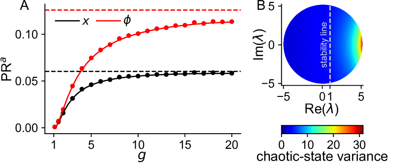
Figure 2: (a) Effective dimension $\text{PR}^{a}$ for $a\in\{x,\phi\}$. Lines: theory. Dots: simulations of size $N=2500$. Median values over 50 disorder realizations are shown. (b) Activity variance in the chaotic state along eigenmodes of the stability matrix at the trivial fixed point with $g=5$. Locally unstable modes with large real part have far greater variance in the chaotic state than those with small real part.

We now specialize to the model of Sompolinsky et al. (1988), with $T[x](t)=(1+\partial_{t})x(t)$ and $\phi(\cdot)=\tanh(\cdot)$, for which the single- and two-site pictures can be treated analytically (Appendix C). This model is chaotic for $g>1$. We use Eqs. 3 and Dimension of Activity in Random Neural Networks to probe the structure of collective activity in the chaotic state, starting with the effective dimension. Let $\Sigma^{a}_{ij}=\left\langle a_{i}(t)a_{j}(t)\right\rangle_{t}$ denote the covariance matrix of the variables $a\in\{x,\phi\}$ and $\lambda^{a}_{i}$ its eigenvalues. Following Rajan et al. (2010a); Abbott et al. (2011); Gao and Ganguli (2015); Gao et al. (2017); Litwin-Kumar et al. (2017); Recanatesi et al. (2019); Engelken et al. (2020); Recanatesi et al. (2020); Hu and Sompolinsky (2022) (see Huang (2018) for the feedforward-network case), we define the effective dimension as the participation ratio of this spectrum,

$$\text{PR}^{a}=\frac{1}{N}\frac{\left(\sum_{i}\lambda_{i}^{a}\right)^{2}}{\sum_{i}(\lambda_{i}^{a})^{2}},$$ (15)

where the factor $1/N$ makes this an intensive quantity, $0\leq\text{PR}^{a}\leq 1$. $\text{PR}^{a}$ provides a linear notion of dimensionality, corresponding roughly to the minimal dimension, relative to $N$, of a subspace in which the strange attractor can be embedded with small L₂-norm distortion. This embedding subspace can be obtained from simulation results using principal components analysis (PCA) Gao and Ganguli (2015); Gao et al. (2017); Trautmann et al. (2019). We evaluate $\text{PR}^{a}$ for $N\rightarrow\infty$ by writing the numerator and denominator of Eq. 15 as the squared trace and Frobenius norm, respectively, of $\bm{\Sigma}^{a}$, then expressing these quantities using DMFT order parameters, yielding

$$\text{PR}^{a}=\frac{C^{a}(0)^{2}}{C^{a}(0)^{2}+\psi^{a}(0,0)}.$$ (16)

Evaluating $\psi^{a}(0,0)$ using Eqs. 3 and Dimension of Activity in Random Neural Networks yields agreement with simulations (Fig. 2A). $\text{PR}^{a}$ grows with $g$ as the activity becomes more tempestuous. $\text{PR}^{\phi}>\text{PR}^{x}$, reflecting the dimension-expanding effect of the nonlinearity, studied in feedforward networks Babadi and Sompolinsky (2014); Litwin-Kumar et al. (2017); Huang (2018). Finally, $N\times\text{PR}^{a}\sim N$, consistent with “extensive chaos” Engelken et al. (2020).

In the “Ising limit” $g\rightarrow\infty$, $C^{\phi}(\tau)$, $\psi^{\phi}(\bm{\tau})$, $C^{x}(\tau)/g^{2}$, and $\psi^{x}(\bm{\tau})/g^{4}$ take on limiting forms. As a result, $\text{PR}^{\phi}$ and $\text{PR}^{x}$ saturate at finite values, $\text{PR}^{x}=6.02\%$ and $\text{PR}^{\phi}=12.6\%$ (Fig. 2A, dashed lines; Appendix C). Thus, the effective dimension is bounded substantially below one for arbitrarily large $g$, implying that structured couplings are required to increase the dimension further.

We next study $\text{PR}^{a}$ near the phase transition at $g=1$, defining $\epsilon=g-1\ll 1$. To leading order in $\epsilon$, $C^{a}(0)=\epsilon$ and $\psi^{a}(0,0)=c/\epsilon$ where $c=F(0,0)=4.27$ ($F$ described below). Thus, $\text{PR}^{a}=\epsilon^{3}/c$. This scaling provides an interesting contrast with a linear stability analysis. Stability at the trivial fixed point, $x_{i}(t)=0$, is determined by the spectrum of $\bm{J}$, which, at large $N$, is a uniform disk of radius $g$ Girko (1985); Tao and Vu (2008). The fractional area of the spectrum past the stability line, $\text{Re}(\lambda)=1$, is ${\sim}\epsilon^{3/2}$. By contrast, $\text{PR}^{a}\sim\epsilon^{3}\ll\epsilon^{3/2}$. Thus, locally unstable modes contribute to the chaotic state in a nonuniform manner. Simulations indicate that this nonuniform contribution of modes also holds at finite $\epsilon$ (Fig. 2B).

Temporal structure of cross covariances.—

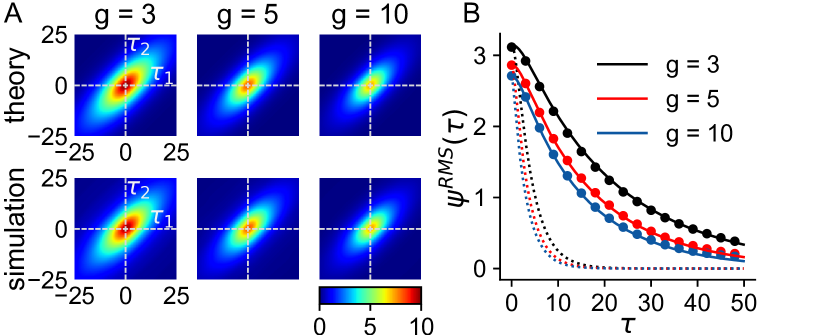
Figure 3: (a) $\psi^{\phi}(\bm{\tau})$. (b) $\psi^{\text{RMS}}(\tau)=\sqrt{\psi^{\phi}(\tau,\tau)}$. Solid lines: theory. Dots: simulations. Dotted lines: rescaled single-unit autocovariance $C^{\phi}(\tau)$ for comparison. $N=2500$. Median values across 50 disorder realizations are shown.

We have focused on the effective dimension, expressed via $\psi^{a}(\bm{\tau})$ for $\bm{\tau}=(0,0)$. We now consider the full $\bm{\tau}$-dependence. Whereas $C^{a}(\tau)$ describes temporal structure of individual units, $\psi^{a}(\bm{\tau})$ describes temporal structure embedded in cross covariances. That $\psi^{a}(\tau,\tau)\neq\psi^{a}(\tau,-\tau)$ reflects the dissipative, time-irreversible nature of the network. The analytical form of $\psi^{\phi}(\bm{\tau})$, Eq. 3, agrees with simulations across $\bm{\tau}$ (Fig. 3A, B). Near the phase transition,

$$\psi^{a}(\bm{\tau})=\frac{1}{\epsilon}F\left(\epsilon^{2}\tau_{+},\>\epsilon\tau_{-}\right),\>\>\tau_{\pm}=({\tau_{1}\pm\tau_{2}})/\sqrt{2},$$ (17)

where $F(\bm{\tau})$ is a decaying order-one function (Appendix C). The timescale of $\psi^{a}(\bm{\tau})$ along the anti-diagonal, ${\tau_{1}=-\tau_{2}}$, is ${\sim}1/\epsilon$, in agreement with the single-unit timescale Sompolinsky et al. (1988). Strikingly, the timescale along the diagonal, ${\tau_{1}=\tau_{2}}$, is ${\sim}1/\epsilon^{2}$, longer than the single-unit timescale by a (diverging) factor of $1/\epsilon$. This $1/\epsilon^{2}$ timescale is in agreement with the inverse Lyapunov exponent Sompolinsky et al. (1988). This long timescale is also present at finite $\epsilon$: defining ${\psi^{\text{RMS}}(\tau)=\sqrt{\psi^{\phi}(\tau,\tau)}}$, we find that $\psi^{\text{RMS}}(\tau)$ has a much slower decay than $C^{\phi}(\tau)$ far from the transition (Fig. 3B).

As this long timescale is not present in individual units, it must arise in collective activity. This motivated us to examine, in simulations, the timescales of collective modes obtained by PCA. The timescales of PCs decrease across the variance-ranked PC index, implying that slow modes account for the most variance. As expected, the leading PCs have timescales many times longer than those of individual units (Fig. A.1A). The density of timescales, $p(\tau)$, has an exponential tail. If this exponential form persists for $N\rightarrow\infty$, the timescales of leading PCs should diverge as ${\sim}\log N$. Simulating networks with sizes spanning two decades confirmed this (Fig. A.1B). Thus, long timescales emerge in unstructured networks, albeit with only a $\log N$ divergence. Unlike in prior proposals (e.g., Litwin-Kumar and Doiron (2012); Stern et al. (2014); Martí et al. (2018); Berlemont and Mongillo (2022)), these long timescales are not visible in individual units, but arise at the collective level through the temporal structure of correlations.

Differential contributions to cross covariances.—The cavity picture provides a partitioning of cross covariances into three sources, each contributing to $C_{00^{\prime}}^{\phi}(\tau)$ at leading order, $1/\sqrt{N}$, in Eq. 8 (upon taking the inverse Fourier transform). First, units $0$ and $0^{\prime}$ receive input from the same reservoir units, inducing a correlation between the cavity fields (Eq. 8, $C^{\eta}_{00^{\prime}}(\tau)$ term). Second, units $0$ and $0^{\prime}$ have direct connections (Eq. 8, delta-function terms in $F_{00^{\prime}}(\tau)$ and $F_{0^{\prime}0}(\tau)$). Third, unit $0^{\prime}$ projects to the reservoir, producing reverberating activity read out by unit $0$, and vice versa (Eq. 8, non-delta-function terms in $F_{00^{\prime}}(\tau)$ and $F_{0^{\prime}0}(\tau)$). Isolating the terms in $\psi^{\phi}(\bm{\tau})$ corresponding to these three sources reveals that cavity-field correlations dominate near the phase transition, with the other two becoming larger further away from the transition (Fig. A.2). Direct connections induce the shortest-timescale correlation. Reverberatory activity induces a slower correlation peaked at finite time lag. Cavity fields provide the slowest correlation.

Structured disorder.—Neural circuits undergo synaptic plasticity during learning. Thus, a key question is how structure in $\bm{J}$ shapes collective activity. Our calculation offers a natural method of incorporating structure in $\bm{J}$, namely, by enforcing it in the couplings involving cavity units ($0$ or $0^{\prime}$) when self-consistently determining the two-point functions of Eq. 10. This works when the structure in $\bm{J}$ is local in the sense that the statistical structure of the entire $\bm{J}$ matrix is fully characterized by its effect on the couplings involving the cavity units.

To demonstrate this, we calculated $\psi^{\phi}(\bm{\tau})$ under partially symmetric structure in the couplings, ${\left\langle J_{ij}J_{ji}\right\rangle=g^{2}\rho/N}$, where $\rho$ is a symmetry parameter. In this case, $\psi^{\phi}(\bm{\tau})$ has the same form as Eq. 3 but with

$$M(\bm{\omega})\rightarrow M(\bm{\omega})\frac{1-\left|2\pi\sigma\left(S^{\phi}(\omega_{1})\right)^{*}S^{\phi}(\omega_{2})\right|^{2}}{\left|1-2\pi\sigma\left(S^{\phi}(\omega_{1})\right)^{*}S^{\phi}(\omega_{2})\right|^{2}},$$ (18)

where $\sigma=g^{2}\rho$ (Appendix D). Additionally, rather than being negligible, the on-diagonal kernels $F_{00}(t,t^{\prime})$ and $F_{0^{\prime}0^{\prime}}(t,t^{\prime})$ are self-averaging with mean $\sqrt{N}\sigma S^{\phi}(t-t^{\prime})$, resulting in an order-one self-coupling in the single-site problem. The equivalence of symmetric structure and an effective self-coupling is likely generic (e.g., such a term arises in networks with ongoing Hebbian plasticity but with the two-point function, rather than the linear response function, serving as the self-coupling kernel Clark and Abbott (2023)).

Our theory yields agreement of $\text{PR}^{\phi}$ and $\psi^{\phi}(\bm{\tau})$ with simulations (Fig. A.3). The effective dimension, $\text{PR}^{\phi}$, has a nontrivial relationship with the symmetry parameter $\rho$: near $\rho=0$, increasing $\rho$ increases or decreases PR^ϕ depending on whether $g$ is small or large, respectively; for all $g$, making $\rho$ sufficiently large decreases PR^ϕ.

Certain types of nonlocal structure can be handled with an expanded set of order parameters. One example is an intensive number groups of units with parameterized within- and across-group coupling statistics, modeling cell types in neural circuits (e.g., excitatory and inhibitory neurons). This could be generalized to a continuous group index, modeling spatial connectivity gradients. We find it unlikely that structure in $\bm{J}$ with nontrivial global constraints (e.g., orthogonality) could be handled by our cavity approach.

Discussion.—We calculated the structure of time-lagged cross covariances in high-dimensional nonlinear dynamical systems with quenched disorder, allowing us to probe collective features of activity in chaotic neural networks. Prior studies have analyzed cross covariances in noise-driven linear models with nonchaotic dynamics Ginzburg and Sompolinsky (1994); Grytskyy et al. (2013); Dahmen et al. (2019); Recanatesi et al. (2019); Shi et al. (2022). In this case, our theory readily recovers the frequency-dependent effective dimension ${\text{PR}^{x}(\omega)=(1-2\pi g^{2}|S^{x}(\omega)|^{2})^{2}}$ (see, e.g., Eqs. 10, 21 of Hu and Sompolinsky (2022), who derived this from random matrix theory). While we used a cavity approach, deriving our results from fluctuations around the saddle point of a path integral would be interesting Crisanti and Sompolinsky (2018); Segadlo et al. (2021); Grosvenor and Jefferson (2022).

Our calculation is agnostic about the single-unit dynamics $T[\cdot]$ and can account for structure in $\bm{J}$. It will be interesting to see how the dimension of activity is shaped by both types of structure. An important extension will be to incorporate time-dependent inputs, which can suppress chaos, an effect crucial to learning Molgedey et al. (1992); Sussillo and Abbott (2009); Rajan et al. (2010b); Schuecker et al. (2018). In the case of inputs with low-dimensional structure, one expects a collapse from extensive to intensive effective dimension when chaos is suppressed.

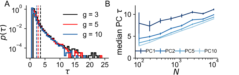
Figure A.1: Timescales of $\phi$ principal components (PCs). (a) Density of PC timescales (autocovariance FWHM) in simulations. Dashed lines: single-unit timescales. $N=2500$, 50 disorder realizations. (b) Timescales of leading PCs vs. $N$. $g=10$. Median timescales across 50 disorder realizations are shown. Error bars: standard error of the mean.

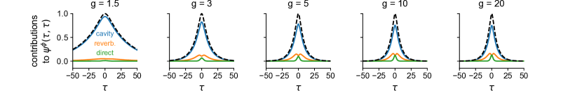
Figure A.2: Relative contributions to $\psi^{\phi}(\tau,\tau)$ from distinct terms in the two-site cavity picture, namely, cavity field correlations (blue), reverberatory activity in the reservoir (orange), and direct coupling (green). Dashed line: $\psi^{\phi}(\tau,\tau)/\psi^{\phi}(0,0)$.

Appendix A: Furutsu-Novikov theorem.—Let ${T[x](t)=\eta(t)}$ where $\eta(t)$ is Gaussian with two-point function $C^{\eta}(t,t^{\prime})$. Let $S^{\phi}(t,t^{\prime})=\left\langle{\delta\phi(t)}/{\delta\eta(t^{\prime})}\right\rangle_{\eta}$, $\phi(t)=\phi(x(t))$. This can be expressed as a functional integral,

$$S^{\phi}(t,t^{\prime})=\int\mathcal{D}\eta e^{-S[\eta]}\frac{\delta\phi(t)}{\delta\eta(t^{\prime})},$$ (19)

where $S[\eta]=\frac{1}{2}\int ds\int ds^{\prime}[C^{\eta}]^{-1}(s,s^{\prime})\eta(s)\eta(s^{\prime})+\text{const}$. We write ${\mathcal{D}\eta=d\eta({\neg t^{\prime}})d\eta(t^{\prime})}$, where $d\eta({\neg t^{\prime}})$ is the measure over all points on $\eta$ excluding $\eta(t^{\prime})$. The integral over $\eta(t^{\prime})$ can be evaluated via scalar integration by parts,

$$\int d\eta(t^{\prime})e^{-S[\eta]}\frac{\delta\phi(t)}{\delta\eta(t^{\prime})}\\ =\int ds[C^{\eta}]^{-1}(t^{\prime},s)\int d\eta(t^{\prime})e^{-S[\eta]}\eta(s)\phi(t),$$ (20)

where the boundary term vanishes for positive definite $C^{\eta}(t,t^{\prime})$. Reintroducing the $d\eta(\neg t^{\prime})$ integration gives

$$S^{\phi}(t,t^{\prime})=\int ds[C^{\eta}]^{-1}(t^{\prime},s)C^{\eta\phi}(s,t),$$ (21)

where $C^{\eta\phi}(s,t)=\left\langle\eta(s)\phi(t)\right\rangle_{\eta}$. Assuming stationarity, we define $C^{\eta}(\tau)=C^{\eta}(t,t+\tau)$, $C^{\eta\phi}(\tau)=C^{\eta\phi}(t,t+\tau)$ and $S^{\phi}(\tau)=S^{\phi}(t,t-\tau)$. Then, $S^{\phi}(\tau)=([C^{\eta}]^{-1}\ast C^{\eta\phi})(\tau)$. In Fourier space, $S^{\phi}(\omega)=C^{\eta\phi}(\omega)/C^{\eta}(\omega)$.

Appendix B: Deriving Eq. 8.—We first write a solution to Eq. 5 accurate to first-order in $1/\sqrt{N}$,

$$\phi_{\mu} (t)=\phi^{\text{free}}_{\mu}(t)$$ (22)

$$+\frac{1}{\sqrt{N}}\int^{t}dt^{\prime}S^{\phi}_{\mu\mu}(t,t^{\prime})\int^{t^{\prime}}dt^{\prime\prime}\sum_{\nu}F_{\mu\nu}(t^{\prime},t^{\prime\prime})\phi^{\text{free}}_{\nu}(t^{\prime\prime}),$$

where $T[x^{\text{free}}_{\mu}](t)=\eta_{\mu}(t)$ and $\phi^{\text{free}}_{\mu}(t)=\phi(x^{\text{free}}_{\mu}(t))$. We multiply the $0$ and $0^{\prime}$ components and $t$-average, working to first order in $1/\sqrt{N}$. The two cross terms arising from $\phi^{\text{free}}_{\mu}(t)$ and the integral terms are readily evaluated by noting that the $0$ and $0^{\prime}$ components decouple under the time average to zeroth order in $1/\sqrt{N}$, yielding the second and third terms in Eq. 8. The nontrivial step is to evaluate $\left\langle\phi^{\text{free}}_{0}(t)\phi^{\text{free}}_{0^{\prime}}(t+\tau)\right\rangle_{t}$. Since $\eta_{0}(t)$ and $\eta_{0^{\prime}}(t)$ can be treated as jointly temporally Gaussian with cross covariance $C^{\eta}_{00^{\prime}}(\tau)\sim 1/\sqrt{N}$, we Taylor expand $\left\langle\phi^{\text{free}}_{0}(t)\phi^{\text{free}}_{0^{\prime}}(t+\tau)\right\rangle_{t}$ in $C^{\eta}_{00^{\prime}}(\tau)$ via Price’s theorem Price (1958), which states (in a sufficiently abstract form) that, for $\bm{x}\sim\mathcal{N}(\bm{0},\bm{\Sigma})$ and a function $F(\bm{x})$,

$$\frac{\partial}{\partial\Sigma_{ij}}\left\langle F(\bm{x})\right\rangle_{\bm{x}}=\left\langle\frac{\partial^{2}F(\bm{x})}{\partial_{x_{i}}\partial_{x_{j}}}\right\rangle_{\bm{x}},$$ (23)

which is apparent upon writing the Gaussian integral corresponding to the LHS in Fourier space. Applying the functional version of this gives the first-order expansion

$$\left\langle\phi^{\text{free}}_{0}(t)\phi^{\text{free}}_{0^{\prime}}(t+\tau)\right\rangle_{t}$$

$$=\int ds\int ds^{\prime}\left\langle\frac{\delta\phi^{\text{free}}_{0}(t)}{\delta\eta_{0}(s)}\frac{\delta\phi^{\text{free}}_{0^{\prime}}(t+\tau)}{\delta\eta_{0^{\prime}}(s^{\prime})}\right\rangle_{t}C_{00^{\prime}}^{\eta}(s^{\prime}-s)$$

$$=\int ds\int ds^{\prime}S^{\phi}(-s)S^{\phi}(\tau-s^{\prime})C^{\eta}_{00^{\prime}}(s^{\prime}-s).$$ (24)

Denoting this by $C^{\phi^{\text{free}}}_{00^{\prime}}(\tau)$, we have in Fourier space $C^{\phi^{\text{free}}}_{00^{\prime}}(\omega)=2\pi|S^{\phi}(\omega)|^{2}C^{\eta}_{00^{\prime}}(\omega)$, the first term in Eq. 8.

Appendix C: Sompolinsky et al. DMFT.—The model of Sompolinsky et al. (1988) is recovered via $T[x](t)=(1+\partial_{t})x(t)$ and $\phi(\cdot)=\tanh(\cdot)$. Squaring the single-site picture, $(1+\partial_{t})x(t)=\eta(t)$, and averaging over $\eta$ reveals that $C^{x}(\tau)$ obeys Newtonian dynamics in a Mexican-hat potential, $V(C^{x})$. $C^{x}(\tau)$ is obtained by numerically integrating this equation of motion. Then, $C^{\phi}(\tau)$ is given in Fourier space by ${C^{\phi}(\omega)=(1+\omega^{2})C^{x}(\omega)/g^{2}}$. The linear responses are $S^{x}(\omega)=1/(1+i\omega)$, $S^{\phi}(\omega)=\alpha/(1+i\omega)$ ($\alpha=\left\langle\phi^{\prime}(x)\right\rangle_{\eta}$). Defining $X(\bm{\omega})=(1+i\omega_{1})(1+i\omega_{2})$ and $\nu=g^{2}\alpha^{2}$,

$$\psi^{\phi}(\bm{\omega}) =\left(\left|\frac{X(\bm{\omega})}{X(\bm{\omega})-\nu}\right|^{2}-1\right)C^{\phi}(\omega_{1})C^{\phi}(\omega_{2}),$$ (25a)

$$\psi^{x}(\bm{\omega}) =\left(\frac{2|X(\bm{\omega})|^{2}-\nu^{2}}{\left|X(\bm{\omega})-\nu\right|^{2}}-1\right)C^{x}(\omega_{1})C^{x}(\omega_{2}).$$ (25b)

In evaluating Eq. Dimension of Activity in Random Neural Networks to obtain Eq. 25b, we noted that ${C^{x\phi}(\omega)=\alpha C^{x}(\omega)}$ due to the Gaussianity of $x$.

Limit of ${g\rightarrow 1^{+}}$: Near the phase transition, $C^{x}(0)\sim\epsilon$ ($\epsilon=g-1$). Taylor expanding $V(C^{x})$ to fourth order in $C^{x}$ and analytically integrating the resulting equation of motion gives ${C^{x}(\tau)=C^{\phi}(\tau)=\epsilon\>\text{sech}\left(\tau\epsilon/\sqrt{3}\right)}$ to first order in $\epsilon$ Crisanti and Sompolinsky (2018). The large-$\tau$ autocovariance behavior is controlled by the quadratic term in $V(C_{x})$, so including higher-order terms in the Taylor expansion gives corrections decaying faster than ${\sim}1/\epsilon$. Thus, in Fourier space, ${C^{a}(\omega)=({3\pi/2})^{1/2}\text{sech}\left(\sqrt{3}\pi\omega/2\epsilon\right)}$ at leading order in $\epsilon$. Noting that ${\nu=1+V^{\prime\prime}(0)}$, we have, from the expanded potential, ${\nu=1-\epsilon^{2}/3}$ at leading nontrivial order. The divergent contributions to the inverse transforms of both $\psi^{x}(\bm{\omega})$ and $\psi^{\phi}(\bm{\omega})$ come from the term ${C^{a}(\omega_{1})C^{a}(\omega_{2})/|X(\bm{\omega})-\nu|^{2}}$. This contribution is

$$\hphantom{a}\psi^{a}(\bm{\tau})=\frac{3}{4}\int d\bm{\omega}e^{i\epsilon\bm{\omega}^{T}\bm{\tau}}\frac{\text{sech}\left(\frac{\sqrt{3}\pi\omega_{1}}{2}\right)\text{sech}\left(\frac{\sqrt{3}\pi\omega_{2}}{2}\right)}{\epsilon^{2}(1/3-\omega_{1}\omega_{2})^{2}+(\omega_{1}+\omega_{2})^{2}}.$$ (26)

Along the anti-diagonal, $\omega_{1}+\omega_{2}=0$, the integrand diverges as ${\sim}1/\epsilon^{2}$. The divergent part is a ridge with thickness ${\sim}\epsilon$, corresponding to the first and second terms in the denominator having similar magnitudes. The ${\sim}1/\epsilon^{2}$ height and ${\sim}\epsilon$ thickness give a ${\sim}1/\epsilon$ divergence of $\psi^{a}(\bm{\tau})$. Defining $\omega_{\pm}=(\omega_{1}\pm\omega_{2})/\sqrt{2}$, we rotate the ridge onto the $\omega_{-}$ axis. The ${\sim}\epsilon$ thickness of the ridge along the $\omega_{+}$ axis suggests replacing $\omega_{+}\rightarrow\epsilon\omega_{+}$, yielding

$$\psi^{a}(\bm{\tau}) =\frac{1}{\epsilon}\int d\bm{\omega}_{\pm}e^{i\left(\epsilon^{2}\omega_{+}\tau_{+}+\epsilon\omega_{-}\tau_{-}\right)}\frac{F(\omega_{+},\omega_{-})}{2\pi},$$ (27a)

$$F(\bm{\omega}_{\pm}) =\frac{3\pi}{2}\frac{\text{sech}^{2}\left(\frac{\sqrt{3}\pi\omega_{-}}{2^{3/2}}\right)}{\left(1/3+\omega_{-}^{2}/2\right)^{2}+2\omega_{+}^{2}},$$ (27b)

where $\tau_{\pm}=({\tau_{1}\pm\tau_{2}})/{\sqrt{2}}$ as defined in the main text.

Limit of $g\rightarrow\infty$: Defining $\bar{C}^{x}(\tau)=C^{x}(\tau)/g^{2}$, the Newtonian dynamics in this limit approach ${\partial_{\tau}^{2}\bar{C}^{x}(\tau)=\bar{C}^{x}(\tau)-({2}/{\pi})\arcsin\left({\bar{C}^{x}(\tau)}/{\bar{C}^{x}(0)}\right)}$ where $\bar{C}^{x}(0)=2(1-2/\pi)$ Crisanti and Sompolinsky (2018). Meanwhile, $\nu=1/(\pi-2)$. Numerically integrating these dynamics allows us to evaluate Eq. 25 numerically, producing the saturating values of $\text{PR}^{a}$ given in the main text.

Appendix D: Partially symmetric disorder.—For finite ${\sigma=g^{2}\rho}$, $\left\langle F_{\mu\mu}(t,t^{\prime})\right\rangle_{\bm{J}}=\sqrt{N}\sigma S^{\phi}(t-t^{\prime})$, modifying the single-site picture by introducing an order-one self-coupling. This self-coupling can be absorbed into the dynamics functional by replacing $T[\cdot]$ with

$$T_{\sigma}[x](t)=T[x](t)+\sigma\int_{-\infty}^{t}dt^{\prime}S^{\phi}(t-t^{\prime})\phi(t^{\prime}).$$ (28)

In our case, ${T[x](t)=(1+\partial_{t})x(t)}$. We solve the single-site DMFT numerically, using the Furutsu-Novikov theorem to evaluate $S^{\phi}(\tau)$. We now self-consistently determine the two-point functions of Eq. 10 under correlated disorder. $\Gamma_{F_{00^{\prime}}F_{00^{\prime}}}(\bm{\omega})$ and $\Gamma_{C^{\eta}_{00^{\prime}}C^{\eta}_{00^{\prime}}}(\bm{\omega})$ are the same as for of i.i.d. disorder. Rather than vanishing, we have also

$$\Gamma_{F^{*}_{00^{\prime}}F_{0^{\prime}0}}(\bm{\omega})=\frac{\sigma}{2\pi\left(1-2\pi\sigma(S^{\phi}(\omega_{1}))^{*}S^{\phi}(\omega_{2})\right)},$$ (29a)

$$\Gamma_{F^{*}_{00^{\prime}}C^{\eta}_{00^{\prime}}}(\bm{\omega})$$ (29b)

$$=(2\pi)^{2}\Gamma_{F_{00^{\prime}}F_{00^{\prime}}}^{*}(\bm{\omega})\Gamma_{F^{*}_{00^{\prime}}F_{0^{\prime}0}}(\bm{\omega})(S^{\phi}(\omega_{1}))^{*}C^{\phi}(\omega_{2}).$$

Using these when squaring and $\bm{J}$-averaging Eq. 8 yields the solution for $\psi^{\phi}(\bm{\omega})$, Eq. 18. The DMFT predictions for $\text{PR}^{\phi}$ and $\psi^{\phi}(\bm{\tau})$ agree with simulations (Fig. A.3).

For $\rho$ approaching unity, this model Martí et al. (2018) and related models Berlemont and Mongillo (2022) have been reported to exhibit temporally nonstationary, “glassy” dynamics, and it is possible that nonstationary behavior appears for $\rho<1$. Our calculation assumes temporal stationarity, but nevertheless matches simulations up to $\rho=0.6$ (modulo small discrepancies that are likely attributable to numerics). Numerically solving the single-site DMFT for larger values of $\rho$ is challenging due to the rapid growth of the autocorrelation timescale with $\rho$.

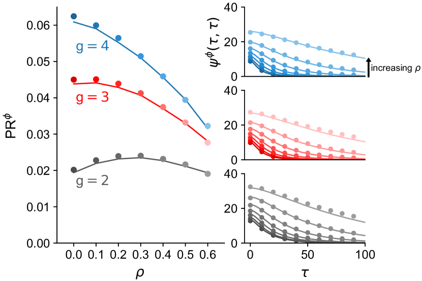
Figure A.3: (a) Effective dimension PR^ϕ as a function of $\rho$ for various values of $g$. (b) $\psi^{\phi}(\tau,\tau)$ as a function of $\tau$ for values of $g$ and $\rho$ from (a). Lines: DMFT. Dots: simulations of size $N=7500$, median across 200 realizations.

References

- Sompolinsky et al. (1988) H. Sompolinsky, A. Crisanti, and H.-J. Sommers, Physical Review Letters 61, 259 (1988).
- Stern et al. (2014) M. Stern, H. Sompolinsky, and L. F. Abbott, Physical Review E 90, 062710 (2014).
- Bahri et al. (2020) Y. Bahri, J. Kadmon, J. Pennington, S. S. Schoenholz, J. Sohl-Dickstein, and S. Ganguli, Annual Review of Condensed Matter Physics 11 (2020).
- Poole et al. (2016) B. Poole, S. Lahiri, M. Raghu, J. Sohl-Dickstein, and S. Ganguli, Advances in Neural Information Processing Systems 29 (2016).
- Huang (2018) H. Huang, Physical Review E 98, 062313 (2018).
- Wardak and Gong (2022) A. Wardak and P. Gong, Phys. Rev. Lett. 129, 048103 (2022).
- Le et al. (2015) Q. V. Le, N. Jaitly, and G. E. Hinton, arXiv preprint arXiv:1504.00941 (2015).
- Schoenholz et al. (2016) S. S. Schoenholz, J. Gilmer, S. Ganguli, and J. Sohl-Dickstein, arXiv preprint arXiv:1611.01232 (2016).
- Martens et al. (2021) J. Martens, A. Ballard, G. Desjardins, G. Swirszcz, V. Dalibard, J. Sohl-Dickstein, and S. S. Schoenholz, arXiv preprint arXiv:2110.01765 (2021).
- Roberts et al. (2021) D. A. Roberts, S. Yaida, and B. Hanin, arXiv preprint arXiv:2106.10165 (2021).
- Jaeger and Haas (2004) H. Jaeger and H. Haas, science 304, 78 (2004).
- Maass et al. (2007) W. Maass, P. Joshi, and E. D. Sontag, PLoS Computational Biology 3, e165 (2007).
- Rivkind and Barak (2017) A. Rivkind and O. Barak, Physical Review Letters 118, 258101 (2017).
- Susman et al. (2021) L. Susman, F. Mastrogiuseppe, N. Brenner, and O. Barak, Physical Review Research 3, 013176 (2021).
- Mastrogiuseppe and Ostojic (2018) F. Mastrogiuseppe and S. Ostojic, Neuron 99, 609 (2018).
- Schuessler et al. (2020) F. Schuessler, F. Mastrogiuseppe, A. Dubreuil, S. Ostojic, and O. Barak, Advances in Neural Information Processing Systems 33, 13352 (2020).
- Martin and Mahoney (2021) C. H. Martin and M. W. Mahoney, J. Mach. Learn. Res. 22, 1 (2021).
- Arieli et al. (1996) A. Arieli, A. Sterkin, A. Grinvald, and A. Aertsen, Science 273, 1868 (1996).
- Flyvbjerg et al. (1993) H. Flyvbjerg, K. Sneppen, and P. Bak, Physical Review Letters 71, 4087 (1993).
- Ciuchi et al. (1996) S. Ciuchi, F. De Pasquale, and B. Spagnolo, Physical Review E 54, 706 (1996).
- Aoki et al. (2014) H. Aoki, N. Tsuji, M. Eckstein, M. Kollar, T. Oka, and P. Werner, Reviews of Modern Physics 86, 779 (2014).
- Kadmon and Sompolinsky (2015) J. Kadmon and H. Sompolinsky, Physical Review X 5, 041030 (2015).
- Aljadeff et al. (2015) J. Aljadeff, M. Stern, and T. Sharpee, Physical Review Letters 114, 088101 (2015).
- Chen et al. (2018) M. Chen, J. Pennington, and S. Schoenholz, in International Conference on Machine Learning (PMLR, 2018) pp. 873–882.
- Roy et al. (2019) F. Roy, G. Biroli, G. Bunin, and C. Cammarota, Journal of Physics A: Mathematical and Theoretical 52, 484001 (2019).
- Mignacco et al. (2020) F. Mignacco, F. Krzakala, P. Urbani, and L. Zdeborová, Advances in Neural Information Processing Systems 33, 9540 (2020).
- Keup et al. (2021) C. Keup, T. Kühn, D. Dahmen, and M. Helias, Physical Review X 11, 021064 (2021).
- van Meegen et al. (2021) A. van Meegen, T. Kühn, and M. Helias, Physical Review Letters 127, 158302 (2021).
- Krishnamurthy et al. (2022) K. Krishnamurthy, T. Can, and D. J. Schwab, Physical Review X 12, 011011 (2022).
- De Giuli and Scalliet (2022) E. De Giuli and C. Scalliet, arXiv preprint arXiv:2205.02204 (2022).
- Rajan et al. (2010a) K. Rajan, L. Abbott, and H. Sompolinsky, Advances in Neural Information Processing Systems 23 (2010a).
- Abbott et al. (2011) L. Abbott, K. Rajan, and H. Sompolinsky, in The dynamic brain: an exploration of neuronal variability and its functional significance, edited by M. Ding and D. Glanzman (Oxford University Press, 2011) p. 65–82.
- Recanatesi et al. (2019) S. Recanatesi, G. K. Ocker, M. A. Buice, and E. Shea-Brown, PLoS Computational Biology 15, e1006446 (2019).
- Engelken et al. (2020) R. Engelken, F. Wolf, and L. Abbott, arXiv preprint arXiv:2006.02427 (2020).
- Recanatesi et al. (2020) S. Recanatesi, S. Bradde, V. Balasubramanian, N. A. Steinmetz, and E. Shea-Brown, bioRxiv (2020).
- Hu and Sompolinsky (2022) Y. Hu and H. Sompolinsky, PLoS Computational Biology 18, 1 (2022).
- Jazayeri and Ostojic (2021) M. Jazayeri and S. Ostojic, Current opinion in neurobiology 70, 113 (2021).
- Litwin-Kumar et al. (2017) A. Litwin-Kumar, K. D. Harris, R. Axel, H. Sompolinsky, and L. Abbott, Neuron 93, 1153 (2017).
- Chung et al. (2018) S. Chung, D. D. Lee, and H. Sompolinsky, Physical Review X 8, 031003 (2018).
- Cohen et al. (2020) U. Cohen, S. Chung, D. D. Lee, and H. Sompolinsky, Nature Communications 11, 1 (2020).
- Farrell et al. (2022) M. Farrell, S. Recanatesi, T. Moore, G. Lajoie, and E. Shea-Brown, Nature Machine Intelligence , 1 (2022).
- Sorscher et al. (2021) B. Sorscher, S. Ganguli, and H. Sompolinsky, bioRxiv (2021).
- Cohen and Sompolinsky (2022) U. Cohen and H. Sompolinsky, arXiv preprint arXiv:2203.07040 (2022).
- Sussillo and Abbott (2009) D. Sussillo and L. Abbott, Neuron 63, 544 (2009).
- Ganguli et al. (2012) S. Ganguli, H. Sompolinsky, et al., Annual Review of Neuroscience 35, 485 (2012).
- Gao and Ganguli (2015) P. Gao and S. Ganguli, Current Opinion in Neurobiology 32, 148 (2015).
- Gao et al. (2017) P. Gao, E. Trautmann, B. Yu, G. Santhanam, S. Ryu, K. Shenoy, and S. Ganguli, bioRxiv , 214262 (2017).
- Trautmann et al. (2019) E. M. Trautmann, S. D. Stavisky, S. Lahiri, K. C. Ames, M. T. Kaufman, D. J. O’Shea, S. Vyas, X. Sun, S. I. Ryu, S. Ganguli, et al., Neuron 103, 292 (2019).
- Martí et al. (2018) D. Martí, N. Brunel, and S. Ostojic, Physical Review E 97, 062314 (2018).
- Muscinelli et al. (2019) S. P. Muscinelli, W. Gerstner, and T. Schwalger, PLoS computational biology 15, e1007122 (2019).
- Beiran and Ostojic (2019) M. Beiran and S. Ostojic, PLoS computational biology 15, e1006893 (2019).
- Clark and Abbott (2023) D. G. Clark and L. Abbott, arXiv preprint arXiv:2302.08985 (2023).
- Note (1) See Mézard et al. (1987) Ch. V.3 for a two-site cavity approach to spin glasses.
- Agoritsas et al. (2018) E. Agoritsas, G. Biroli, P. Urbani, and F. Zamponi, Journal of Physics A: Mathematical and Theoretical 51, 085002 (2018).
- Mézard et al. (1987) M. Mézard, G. Parisi, and M. A. Virasoro, Spin glass theory and beyond: An Introduction to the Replica Method and Its Applications, Vol. 9 (World Scientific Publishing Company, 1987).
- Advani et al. (2013) M. Advani, S. Lahiri, and S. Ganguli, Journal of Statistical Mechanics: Theory and Experiment 2013, P03014 (2013).
- Note (2) By this, we mean that, for a given realization of , all (cross-)cumulants (under the average) higher than second-order are suppressed by at least . Note that this joint Gaussianity property is not true of the local fields appearing in Eq. 1 due to correlations between and .
- Babadi and Sompolinsky (2014) B. Babadi and H. Sompolinsky, Neuron 83, 1213 (2014).
- Girko (1985) V. L. Girko, Theory of Probability & Its Applications 29, 694 (1985).
- Tao and Vu (2008) T. Tao and V. Vu, Communications in Contemporary Mathematics 10, 261 (2008).
- Litwin-Kumar and Doiron (2012) A. Litwin-Kumar and B. Doiron, Nature Neuroscience 15, 1498 (2012).
- Berlemont and Mongillo (2022) K. Berlemont and G. Mongillo, bioRxiv (2022).
- Ginzburg and Sompolinsky (1994) I. Ginzburg and H. Sompolinsky, Physical review E 50, 3171 (1994).
- Grytskyy et al. (2013) D. Grytskyy, T. Tetzlaff, M. Diesmann, and M. Helias, Frontiers in Computational Neuroscience 7, 131 (2013).
- Dahmen et al. (2019) D. Dahmen, S. Grün, M. Diesmann, and M. Helias, Proceedings of the National Academy of Sciences 116, 13051 (2019).
- Shi et al. (2022) Y.-L. Shi, R. Zeraati, A. Levina, and T. A. Engel, arXiv preprint arXiv:2207.07930 (2022).
- Crisanti and Sompolinsky (2018) A. Crisanti and H. Sompolinsky, Physical Review E 98, 062120 (2018).
- Segadlo et al. (2021) K. Segadlo, B. Epping, A. van Meegen, D. Dahmen, M. Krämer, and M. Helias, arXiv preprint arXiv:2112.05589 (2021).
- Grosvenor and Jefferson (2022) K. Grosvenor and R. Jefferson, SciPost Physics 12, 081 (2022).
- Molgedey et al. (1992) L. Molgedey, J. Schuchhardt, and H. G. Schuster, Physical Review Letters 69, 3717 (1992).
- Rajan et al. (2010b) K. Rajan, L. Abbott, and H. Sompolinsky, Physical Review E 82, 011903 (2010b).
- Schuecker et al. (2018) J. Schuecker, S. Goedeke, and M. Helias, Physical Review X 8, 041029 (2018).
- Price (1958) R. Price, IRE Transactions on Information Theory 4, 69 (1958).