Finite-Time Analysis of Asynchronous Q-learning under Diminishing Step-Size from Control-Theoretic View

Han-Dong Lim Department of Electrical and Engineering, Korea Advanced Institute of Science and Technology (KAIST), Daejeon, 34141, South Korea (limaries30@kaist.ac.kr ,donghwan@kaist.ac.kr )    Donghwan Lee11footnotemark: 1 This work was supported by Institute of Information communications Technology Planning Evaluation (IITP) grant funded by the Korea government (MSIT)(No.2022-0-00469)
Abstract

Q-learning has long been one of the most popular reinforcement learning algorithms, and theoretical analysis of Q-learning has been an active research topic for decades. Although researches on asymptotic convergence analysis of Q-learning have a long tradition, non-asymptotic convergence has only recently come under active study. The main goal of this paper is to investigate new finite-time analysis of asynchronous Q-learning under Markovian observation models via a control system viewpoint. In particular, we introduce a discrete-time time-varying switching system model of Q-learning with diminishing step-sizes for our analysis, which significantly improves recent development of the switching system analysis with constant step-sizes, and leads to $\mathcal{O}\left(\sqrt{\frac{\log k}{k}}\right)$ convergence rate that is comparable to or better than most of the state of the art results in the literature. In the mean while, a technique using the similarly transformation is newly applied to avoid the difficulty in the analysis posed by diminishing step-sizes. The proposed analysis brings in additional insights, covers different scenarios, and provides new simplified templates for analysis to deepen our understanding on Q-learning via its unique connection to discrete-time switching systems.


1 Introduction

Recently, reinforcement learning has shown remarkable performance in complex and challenging domains. In the seminal work [38], the so-called deep Q-learning has achieved human level performance in challenging tasks such as the Atari video games using deep learning based approaches. Since then, there have been major improvements [25, 43, 3, 2] to solve the Atari benchmark problems as well. On the other hand, significant progresses have been made for other various fields such as recommendation system [1], robotics [27], and portfolio management [24] to name just a few.

Developed by Watkins in [49], Q-learning is one of the most widely known reinforcement learning algorithms. Theoretical analysis of Q-learning has been an active research topic for decades. In particular, asymptotic convergence of Q-learning has been successfully established through a series of works [48, 23, 10, 31] based on stochastic approximation theory [10]. Although the asymptotic analysis ensures the essential property, the convergence to a solution, the natural question remains unanswered: does the algorithm make a consistent and quantifiable progress toward an optimal solution? To understand this non-asymptotic behavior, meaningful advances have been made recently [47, 17, 33, 35, 12, 41, 36] as well. Among the promising results, our main concern is the control-theoretic framework [33], which provides a unique switching system [37] perspective of Q-learning. In particular, asynchronous Q-learning with a constant step-size has been naturally formulated as a stochastic discrete-time affine switching system, which has allowed us to transform the convergence analysis into a stability analysis of the switching system model from control theoretic viewpoints. This analysis provides new insights and analysis framework to deepen our understanding on Q-learning via its unique connection to discrete-time switching systems with remarkably simplified proofs. Nevertheless, this work leaved key questions unanswered, which are summarized as follows:

  1. 1.

    The study in [33] provides a finite-time analysis for the averaged iterate of Q-learning rather than the final-time iterate. However, the averaged iterate requires additional steps, and it can slow down the convergence in practice.

  2. 2.

    It only considers a constant step-size, which results in biases in the final solution. On the other hand, a diminishing step-size is more widely used in theoretical analysis to guarantee convergence to a solution without the biases.

  3. 3.

    The analysis in [33] adopts i.i.d. observation models. Although this assumption simplifies the overall analysis, it is too idealistic to reflect real world scenarios.

Motivated from the above discussions, the main goal of this paper is to revisit the non-asymptotic analysis of asynchronous Q-learning [33] from discrete-time switching system viewpoints. Contrary to [33], we consider diminishing step-sizes, Markovian observation models, and the final-time convergence. Our main contributions are summarized below.

Contributions
  1. 1)

    A new finite-time analysis is proposed for asynchronous Q-learning under Markovian observation models and diminishing step-sizes, which answers the key questions that were left unsolved in [33]. The new analysis offers $\mathcal{O}\left(\sqrt{\frac{\log k}{k}}\right)$ convergence rate in terms of number of iterations, which is comparable to or better than most of the state of the art results [12, 35, 41] under Markovian observation models. Finite-time analysis of asynchronous Q-learning has been actively investigated recently in [12, 35, 41] under Markovain observation models. Compared to the previous works, the main differences lie in conditions on the diminishing step-size rules. In particular, our conditions on the diminishing step-sizes are independent of the mixing time, where the mixing time is a quantity that characterizes the convergence speed of the current state-action distribution to the stationary distribution, and it plays an important role in the analysis of stochastic algorithms [12, 41, 35, 15, 16] under Markovian noise scenarios. On the other hand, the previous works [12, 35] employ conditions on step-sizes that depend on the mixing time or the covering time [5], which is another quantity that characterizes the exploration performance. Therefore, the proposed new analysis covers different scenarios. Moreover, some of the previous approaches require deliberate processes to predict the mixing time of the underlying Markov chain [50, 21], which are not required in our approach.

  2. 2)

    We revisit the control theoretic analysis in [33], and consider a diminishing step-size. With the diminishing step-size, it is hard to directly apply the proof techniques in [33] due to time-varying nature of the diminishing step-size, which transfers the underlying linear switching system into a time-varying system, and it is in general much more challenging to analyze. To overcome this difficulty, we develop a new approach mainly based on a domain transformation [30] to a new coordinate, which facilitates analysis of convergence on the negative definite cone. Besides, we also take into account the last-time convergence and Markovian observation models in contrary to [33]. Finally, we stress that our goal is to provide new insights and analysis framework to deepen our understanding on Q-learning via its unique connection to discrete-time switching systems, rather than improving existing convergence rates. In this respect, we view our analysis technique as a complement rather than a replacement for existing techniques for Q-learning.

Related Works

Since Q-learning was developed by Watkins in [49], several advances have been made in a series of works. Here, we summarize related results in the literature.

  1. 1.

    Asymptotic convergence: Convergence of synchronous Q-learning was analyzed for the first time in the original paper [49]. Subsequently, convergence of asynchronous Q-learning was studied in [23, 48] using results in stochastic approximation and contraction mapping property. Moreover, an ordinary differential equation (O.D.E) approach was developed in [10] to prove general stochastic approximations, and applied it to prove convergence of synchronous Q-learning. More recently, [31] developed a switching system model of asynchronous Q-learning, and applied the O.D.E method for its convergence.

  2. 2.

    Non-asymptotic convergence with diminishing step-sizes: The early result in [47] considered state-dependent diminishing step-sizes to study non-asymptotic convergence under independent and identically distributed (i.i.d.) observation models. There are a few works focusing on the Markovian sampling setting together with diminishing step-sizes. In particular, [17] obtained sample complexity to achieve $\epsilon$-optimal solution with high probabilities by extending the convergence analysis of [6]. More recently, [41] considered a general asynchronous stochastic approximation scheme featuring a weighted infinity-norm contractive operator, and proved a bound on its finite-time convergence rate under the Markovian sampling setting. They used the notion of the so-called sufficient exploration and error decomposition with shifted martingale difference sequences. Another recent work in [12] employed the so-called generalized Moreau envelope and the notion of Lyapunov function. The recent study in [35] provided a probability tail bound through refined analysis based on an adaptive step-size, which depends on the number of visits to each state-action pair. Besides, [32] proposed an optimization-based Q-learning that mimics the recent deep Q-learning in [38], and offered new finite-time convergence results.

  3. 3.

    Non-asymptotic convergence with constant step-sizes: The aforementioned works applied time-varying step-sizes such as diminishing or adaptive step-sizes. On the other hand, there are some works dealing with Q-learning under constant step-sizes. For instance, [5, 4] employed the concept of the so-called covering time, $t_{\text{cover}}$, to derive mean squared error bounds. Using similar approaches as in the diminishing step-size analysis [35], [12] proposed new convergence analysis under Markovian observation models. More recently, [33] developed a discrete-time switching system model of asynchronous Q-learning to compute a convergence rate of averaged iterated under i.i.d. observation model.

  4. 4.

    Control system approach: Finally, it is worth summarizing related studies based on control system frameworks. Dynamical system perspectives of reinforcement learning and general stochastic iterative algorithms have a long tradition, and they date back to O.D.E analysis [9, 29, 8, 10]. Recently, [22] studied asymptotic convergence of temporal difference learning (TD-learning) [46] based on a Markovian jump linear system model. They tailored Markovian jump linear system theory developed in the control community to characterize exact behaviors of the first and second order moments of TD-learning algorithms. The paper [31] studied asymptotic convergence of Q-learning [49] through a continuous-time switched linear system model [37]. A finite-time analysis of Q-learning was also investigated in [33] using discrete-time switched linear system models.

The paper is organized as follows.

  1. 1.

    Section 2 provides preliminary backgrounds on Markov decision process, dynamic system, Q-learning, essential notations and definitions used throughout the paper.

  2. 2.

    In Section 3, we introduce a dynamic system model of Q-learning. In particular, Q-learning is represented by a stochastic linear time-varying switching system with an affine input term.

  3. 3.

    Section 4 is devoted to analysis of the lower comparison system. We provide essential properties of the lower comparison system, and prove its convergence through a domain transformation under i.i.d. observation model.

  4. 4.

    In Section 5, convergence of the upper comparison system is given under i.i.d. observation model.

  5. 5.

    Based on the results in the previous two sections, the convergence of the lower and upper comparison systems, Section 6 provides a proof of the convergence of Q-learning under i.i.d. observation model.

  6. 6.

    Section 7 extends the analysis in the previous sections with i.i.d. scenario to Markovian observation case.

  7. 7.

    Finally, the overall results are concluded in Section 8.

2 Preliminaries

2.1 Notations

The adopted notation throughout the paper is as follows: {\mathbb{R}}: set of real numbers; nsuperscript𝑛{\mathbb{R}}^{n}: n𝑛n-dimensional Euclidean space; n×msuperscript𝑛𝑚{\mathbb{R}}^{n\times m}: set of all n×m𝑛𝑚n\times m real matrices; Asuperscript𝐴topA^{\top}: transpose of matrix A𝐴A; A0succeeds𝐴0A\succ 0 (A0precedes𝐴0A\prec 0, A0succeeds-or-equals𝐴0A\succeq 0, and A0precedes-or-equals𝐴0A\preceq 0, respectively): symmetric positive definite (negative definite, positive semi-definite, and negative semi-definite, respectively) matrix A𝐴A; xy𝑥𝑦x\leq y and xy𝑥𝑦x\geq y for vectors x,y𝑥𝑦x,y: element-wise inequalities; I𝐼I: identity matrix with appropriate dimensions; ρ()𝜌\rho(\cdot): spectral radius; for any matrix A𝐴A, [A]ijsubscriptdelimited-[]𝐴𝑖𝑗[A]_{ij} is the element of A𝐴A in i𝑖i-th row and j𝑗j-th column; λmin(A)subscript𝜆𝐴\lambda_{\min}(A) and λmax(A)subscript𝜆𝐴\lambda_{\max}(A) for any symmetric matrix A𝐴A: the minimum and maximum eigenvalues of A𝐴A, respectively; σmin(A)subscript𝜎𝐴\sigma_{\min}(A) and σmax(A)subscript𝜎𝐴\sigma_{\max}(A): minimum and maximum singular value of matrix A𝐴A, respectively; |𝒮|𝒮|{\cal S}|: cardinality of a finite set 𝒮𝒮\cal S.

2.2 Markov decision process

In this paper, we consider an infinite horizon Markov decision process (MDP). It consists of a tuple =(𝒮,𝒜,P,r,γ)𝒮𝒜𝑃𝑟𝛾\mathcal{M}=(\mathcal{S},\mathcal{A},P,r,\gamma), where 𝒮𝒮\mathcal{S} and 𝒜𝒜\mathcal{A} represent finite state and action spaces, respectively, P(s|s,a)𝑃conditionalsuperscript𝑠𝑠𝑎P(s^{\prime}|s,a) denotes the transition probability when action a𝑎a is taken at state s𝑠s, and transition occurs to ssuperscript𝑠s^{\prime}, r:𝒮×𝒜×𝒮:𝑟𝒮𝒜𝒮r:\mathcal{S}\times\mathcal{A}\times\mathcal{S}\rightarrow\mathbb{R} denotes the reward function, and γ(0,1)𝛾01\gamma\in(0,1) is the discount factor. With a stochastic policy π:𝒮𝒫(𝒜):𝜋𝒮𝒫𝒜\pi:\mathcal{S}\rightarrow\mathcal{P}(\mathcal{A}), where 𝒫(𝒜)𝒫𝒜\mathcal{P}(\mathcal{A}) is the set of probability distributions over 𝒜𝒜\mathcal{A}, agent at the current state s𝑠s selects an action aπ(|s)a\sim\pi(\cdot|s), then the agent’s state changes to the next state sP(|s,a)s^{\prime}\sim P(\cdot|s,a), and receives reward r:=r(s,a,s)assign𝑟𝑟𝑠𝑎superscript𝑠r:=r(s,a,s^{\prime}). For a deterministic policy π:𝒮𝒜:𝜋𝒮𝒜\pi:\mathcal{S}\to\mathcal{A}, π(s)𝒜𝜋𝑠𝒜\pi(s)\in\mathcal{A} is selected without randomness at state s𝑠s.

The objective of the Markov decision problem (MDP) is to find an optimal policy, denoted by $\pi^{*}$, such that the cumulative discounted rewards over infinite time horizons is maximized, i.e.,

$\displaystyle\pi^{*}:=\operatorname*{arg\,max}_{\pi}{\mathbb{E}}\left[\left.\sum_{k=0}^{\infty}{\gamma^{k}r_{k}}\right|\pi\right],$

where $(s_{0},a_{0},r_{0},s_{1},a_{1},r_{1},\ldots)$ is a state-action trajectory generated by the Markov chain under policy $\pi$, $r_{k}$ denotes the reward received at time $k$ (will be detailed later), and ${\mathbb{E}}[\cdot|\pi]$ is an expectation conditioned on the policy $\pi$.

The Q-function under policy $\pi$ is defined as

$\displaystyle Q^{\pi}(s,a)={\mathbb{E}}\left[\left.\sum_{k=0}^{\infty}{\gamma^{k}r_{k}}\right|s_{0}=s,a_{0}=a,\pi\right],\quad(s,a)\in{\cal S}\times{\cal A},$

and the optimal Q-function is defined as $Q^{*}(s,a)=Q^{\pi^{*}}(s,a)$ for all $(s,a)\in{\cal S}\times{\cal A}$. Once $Q^{*}$ is obtained, then an optimal policy can be retrieved by the greedy action with respect to $Q^{*}$, i.e., $\pi^{*}(s)=\operatorname*{arg\,max}_{a\in{\cal A}}Q^{*}(s,a)$. Throughout, we assume that the MDP is ergodic [34] so that the stationary state distribution exists, is unique, and the Markov decision problem is well posed.

It is known that the optimal Q-function satisfies Bellman equation expressed as follows:

$\displaystyle Q^{*}(s,a)$
=\displaystyle= 𝔼[rk+1+maxak+1𝒜γQ(sk+1,ak+1)|sk=s,ak=a].𝔼delimited-[]formulae-sequencesubscript𝑟𝑘1conditionalsubscriptsubscript𝑎𝑘1𝒜𝛾superscript𝑄subscript𝑠𝑘1subscript𝑎𝑘1subscript𝑠𝑘𝑠subscript𝑎𝑘𝑎\displaystyle\mathbb{E}\left[\left.r_{k+1}+\max_{a_{k+1}\in\mathcal{A}}\gamma Q^{*}(s_{k+1},a_{k+1})\right|s_{k}=s,a_{k}=a\right]. (1)

Finally, some notations related to MDP are summarized as follows: $P_{a}\in\mathbb{R}^{|{\mathcal{S}}|\times|{\mathcal{S}}|},a\in{\mathcal{A}}$ is the state transition matrix when action $a$ is taken at state $s\in\mathcal{S}$. Likewise, $R_{a}\in\mathbb{R}^{|\mathcal{S}|},a\in\mathcal{A}$ is the reward vector when action $a$ is taken at state $s\in\mathcal{S}$, i.e., $R_{a}(s):={\mathbb{E}}[r(s,a,s^{\prime})|s,a],s\in{\mathcal{S}}$. Moreover, the notation $Q_{a}:=Q(\cdot,a)\in{\mathbb{R}}^{|{\mathcal{S}}|},a\in{\mathcal{A}}$ will be adopted throughout the paper.

2.3 Switching system

In this subsection, we briefly review the switching system, which will play an important role in this paper. The switching system is a special form of nonlinear systems, and hence, we first consider the nonlinear system

xk+1=f(xk),x0=zn,k{0,1,},formulae-sequenceformulae-sequencesubscript𝑥𝑘1𝑓subscript𝑥𝑘subscript𝑥0𝑧superscript𝑛𝑘01\displaystyle x_{k+1}=f(x_{k}),\quad x_{0}=z\in{\mathbb{R}}^{n},\quad k\in\{0,1,\ldots\}, (2)

where $x_{k}\in{\mathbb{R}}^{n}$ is the state and $f:{\mathbb{R}}^{n}\to{\mathbb{R}}^{n}$ is a nonlinear mapping. An important concept in dealing with the nonlinear system is the equilibrium point. A point $x=x^{*}$ in the state-space is said to be an equilibrium point of (2) if it has the property that whenever the state of the system starts at $x^{*}$, it will remain at $x^{*}$ [26]. For (2), the equilibrium points are the real roots of the equation $f(x)=0$. The equilibrium point $x^{*}$ is said to be globally asymptotically stable if for any initial state $x_{0}\in{\mathbb{R}}^{n}$, $x_{k}\to x^{*}$ as $k\to\infty$.

Next, let us consider the particular nonlinear system, the linear switching system,

xk+1=Aσkxk,x0=zn,k{0,1,},formulae-sequenceformulae-sequencesubscript𝑥𝑘1subscript𝐴subscript𝜎𝑘subscript𝑥𝑘subscript𝑥0𝑧superscript𝑛𝑘01\displaystyle x_{k+1}=A_{\sigma_{k}}x_{k},\quad x_{0}=z\in{\mathbb{R}}^{n},\quad k\in\{0,1,\ldots\}, (3)

where $x_{k}\in{\mathbb{R}}^{n}$ is the state, $\sigma\in{\mathcal{M}}:=\{1,2,\ldots,M\}$ is called the mode, $\sigma_{k}\in{\mathcal{M}}$ is called the switching signal, and $\{A_{\sigma},\sigma\in{\mathcal{M}}\}$ are called the subsystem matrices. The switching signal can be either arbitrary or controlled by the user under a certain switching policy. Especially, a state-feedback switching policy is denoted by $\sigma_{k}=\sigma(x_{k})$. A more general class of systems is the affine switching system

$\displaystyle x_{k+1}=A_{\sigma_{k}}x_{k}+b_{\sigma_{k}},\quad x_{0}=z\in{\mathbb{R}}^{n},\quad k\in\{0,1,\ldots\},$

where $b_{\sigma_{k}}\in{\mathbb{R}}^{n}$ is the additional input vector, which also switches according to $\sigma_{k}$. Due to the additional input $b_{\sigma_{k}}$, its stabilization becomes much more challenging.

2.4 Linear time-varying system

In this section, we briefly review the linear time-varying (LTV) system [51]. Let us first consider the continuous-time linear time-invariant (LTI) system

x˙t=Axt,subscript˙𝑥𝑡𝐴subscript𝑥𝑡\displaystyle\dot{x}_{t}=Ax_{t}, (4)

where $x_{t}\in\mathbb{R}^{n}$ is the state, $A\in\mathbb{R}^{n\times n}$ is the system matrix. The asymptotic stability of (4) is completely characterized by the notion called Hurwitz matrix [26, 11], which is defined as follows.

Definition 2.1 (Hurwitz matrix [26, 11]).

A square matrix An×n𝐴superscript𝑛𝑛A\in\mathbb{R}^{n\times n} is called Hurwitz if its real part of eigenvalues are negative.

It is well-known that (4) is asymptotically stable if and only if $A$ is Hurwitz. In general, it is hard to check the Hurwitzness without computing the eigenvalues. Nevertheless, a sufficient condition can be obtained in terms of algebraic relations among entries of the corresponding matrix, which is called the strict diagonal dominance.

Definition 2.2 (Strict diagonal dominance [20]).

A square matrix $A\in\mathbb{R}^{n\times n}$ is said to be strictly diagonally dominant if

$\displaystyle|[A]_{ii}|>\sum\limits_{j\neq i,j=1}^{n}|[A]_{ij}|,\quad\forall{i}\in\{1,2,\dots,n\}.$
Lemma 2.1.

A square matrix $A$ is Hurwitz if it is a strictly row diagonally dominant matrix and the diagonal elements are negative.

The proof of Lemma 2.1 is in Appendix Section 9.1.

A linear time-varying (LTV) system is a class of linear systems defined as

xk+1=Akxk,subscript𝑥𝑘1subscript𝐴𝑘subscript𝑥𝑘\displaystyle x_{k+1}=A_{k}x_{k}, (5)

where $x_{k}\in\mathbb{R}^{n}$ is the state, and $A_{k}\in\mathbb{R}^{n\times n}$ is the time-varying system matrix. Together with switching systems, LTV system models will be used in the analysis of this paper. Stability analysis of LTV systems is much more challenging than a simple linear time-invariant system [11]. For their asymptotic stability, the following sufficient condition will be used in this paper.

Lemma 2.2 ([51], Theorem 1).

The discrete-time LTV system (5) is asymptotically stable if there exists a sequence of positive definite matrices $\{P_{k}\}_{k=0}^{n}$, and positive scalars $\{p_{k}\}_{k=0}^{n}$ such that the following conditions hold for all $k\geq 0$:

  1. 1)

    $A^{\top}_{k}P_{k+1}A_{k}\preceq p_{k}P_{k}$;

  2. 2)

    $\Pi_{k=1}^{n}p_{k}\to 0$ as $n\to\infty$;

  3. 3)

    $c\leq\lambda_{\min}(P_{k})$ for some positive constant $c>0$.

Proof.

Let $V_{k}(x_{k})=x^{\top}_{k}P_{k}x_{k}$ be a time-varying Lyapunov function that satisfies the condition in item 1). Recursively applying the inequality in item 1) leads to

$\displaystyle V_{k}(x_{k})\leq p_{k-1}V_{k-1}(x_{k-1})\leq\left(\prod\nolimits_{i=0}^{k-1}{p_{i}}\right)V_{0}(x_{0}).$

Using item 3), it follows from the last inequality that

$\displaystyle c\left\|{x_{k}}\right\|_{2}^{2}\leq V_{k}(x_{k})\leq\left(\prod\nolimits_{i=0}^{k-1}{p_{i}}\right)V_{0}(x_{0})\leq\left({\prod\nolimits_{i=0}^{k-1}{p_{i}}}\right)\lambda_{\max}(P_{0}),$

which leads to

$\displaystyle\|x_{k}\|_{2}^{2}\leq\left({\prod\nolimits_{i=0}^{k-1}{p_{i}}}\right)\frac{{\lambda_{\max}(P_{0})}}{c}.$

By item 2), we have $\|x_{k}\|_{2}\to 0$ as $k\to\infty$. This completes the proof. ∎

2.5 Matrix notations

In this paper, a linear time-varying switching system model of Q-learning will be used for the analysis. To this end, the following matrix notations will be useful to compactly represent Q-learning into a vector and matrix forms:

P:=[P1P|𝒜|]|𝒮||𝒜|×|𝒮|,R:=[R1R|𝒜|]|𝒮||𝒜|,Q:=[Q1Q|𝒜|]|𝒮||𝒜|.formulae-sequenceassign𝑃matrixsubscript𝑃1subscript𝑃𝒜superscript𝒮𝒜𝒮assign𝑅matrixsubscript𝑅1subscript𝑅𝒜superscript𝒮𝒜assign𝑄matrixsubscript𝑄1subscript𝑄𝒜superscript𝒮𝒜\displaystyle P:=\begin{bmatrix}P_{1}\\ \vdots\\ P_{|{\mathcal{A}}|}\end{bmatrix}\in{\mathbb{R}}^{|{\mathcal{S}}||{\mathcal{A}}|\times|{\mathcal{S}}|},\quad R:=\begin{bmatrix}R_{1}\\ \vdots\\ R_{|{\mathcal{A}}|}\end{bmatrix}\in{\mathbb{R}}^{|{\mathcal{S}}||{\mathcal{A}}|},\quad Q:=\begin{bmatrix}Q_{1}\\ \vdots\\ Q_{|{\mathcal{A}}|}\\ \end{bmatrix}\in{\mathbb{R}}^{|{\mathcal{S}}||{\mathcal{A}}|}.

Under policy $\pi$, we have $P^{\pi}\in\mathbb{R}^{|{\mathcal{S}}||{\mathcal{A}}|\times|{\mathcal{S}}||{\mathcal{A}}|}$ as the state-action transition matrix, i.e.,

$\displaystyle(e_{s}\otimes e_{a})^{\top}P^{\pi}(e_{s^{\prime}}\otimes e_{a^{\prime}})={\mathbb{P}}[s_{t+1}=s^{\prime},a_{t+1}=a^{\prime}|s_{t}=s,a_{t}=a,\pi],$

where $\otimes$ stands for the Kronecker product, and $e_{a}$ and $e_{s}$ to represent $a$-th and $s$-th canonical basis vectors in $\mathbb{R}^{|\mathcal{A}|}$ and $\mathbb{R}^{|\mathcal{S}|}$, respectively.

In this paper, we represent a policy in a matrix form. In particular, for a given policy $\pi$, define the matrix

Ππ:=[(eπ(1)e1)(eπ(|𝒮|)e|𝒮|)]|𝒮|×|𝒮||𝒜|.assignsuperscriptΠ𝜋matrixsuperscripttensor-productsubscript𝑒𝜋1subscript𝑒1topsuperscripttensor-productsubscript𝑒𝜋𝒮subscript𝑒𝒮topsuperscript𝒮𝒮𝒜\displaystyle\Pi^{\pi}:=\begin{bmatrix}(e_{\pi(1)}\otimes e_{1})^{\top}\\ \vdots\\ (e_{\pi(|\mathcal{S}|)}\otimes e_{|\mathcal{S}|})^{\top}\\ \end{bmatrix}\in\mathbb{R}^{|\mathcal{S}|\times|\mathcal{S}||\mathcal{A}|}. (6)

Then, we can prove that for any deterministic policy, $\pi$, we have

ΠπQ=[Q(1,π(1))Q(2,π(2))Q(|𝒮|,π(|𝒮|))].superscriptΠ𝜋𝑄matrix𝑄1𝜋1𝑄2𝜋2𝑄𝒮𝜋𝒮\displaystyle\Pi^{\pi}Q=\begin{bmatrix}{Q(1,\pi(1))}\\ {Q(2,\pi(2))}\\ \vdots\\ {Q(|{\mathcal{S}}|,\pi(|{\mathcal{S}}|))}\\ \end{bmatrix}.

With this $\Pi^{\pi}$, we can prove that for any deterministic policy $\pi$, $P^{\pi}=P\Pi^{\pi}\in\mathbb{R}^{|\mathcal{S}||\mathcal{A}|\times|\mathcal{S}||\mathcal{A}|}$, where $P^{\pi}$ stands for the state-action transition matrix. Using the notations introduced, the Bellman equation in (7) can be compactly written as

Q=γPΠπQQ+R,superscript𝑄𝛾𝑃subscriptΠsubscript𝜋superscript𝑄superscript𝑄𝑅Q^{*}=\gamma P\Pi_{\pi_{Q^{*}}}Q^{*}+R, (7)

where $\pi_{Q^{*}}$ is the greedy policy defined as $\pi_{Q^{*}}(s)=\operatorname*{arg\,max}_{a\in\mathcal{A}}Q^{*}(s,a)$. Moreover, for simplicity of notations, we introduce the following shorthand:

$\displaystyle\Pi_{Q}:=\Pi^{\pi_{Q}},$

when the policy is the greedy policy $\pi_{Q}(s)=\operatorname*{arg\,max}_{a\in\mathcal{A}}Q(s,a)$ with respect to $Q$.

2.6 Revisit Q-learning

This section briefly reviews standard Q-learning and its important properties. Two versions of Q-learning will be investigated in this paper.

Algorithm 1 Q-learning with i.i.d. observation model
1:Initialize $Q_{0}\in{\mathbb{R}}^{|{\cal S}||{\cal A}|}$.
2:Set the step-size $(\alpha_{k})_{k=0}^{\infty}$, and the behavior policy $\beta$.
3:for iteration $k=0,1,\ldots$ do
4:     Sample $s_{k}\sim p$ and $a_{k}\sim\beta$
5:     Sample $s_{k}^{\prime}\sim P(s_{k},a_{k},\cdot)$ and $r_{k}=r(s_{k},a_{k},s_{k}^{\prime})$
6:     Update $Q_{k+1}(s_{k},a_{k})=Q_{k}(s_{k},a_{k})+\alpha_{k}\{r_{k}+\gamma\max_{u\in{\cal A}}Q_{k}(s_{k}^{\prime},u)-Q_{k}(s_{k},a_{k})\}$
7:end for
Algorithm 2 Q-learning with Markovian observation model
1:Initialize $Q_{0}\in{\mathbb{R}}^{|{\cal S}||{\cal A}|}$.
2:
3:Set the step-size $(\alpha_{k})_{k=0}^{\infty}$, and the behavior policy $\beta$.
4:Sample $s_{0}\sim p_{0}$
5:for iteration $k=0,1,\ldots$ do
6:     Sample $a_{k}\sim\beta$
7:     Sample $s_{k+1}\sim P(s_{k},a_{k},\cdot)$ and $r_{k}=r(s_{k},a_{k},s_{k+1})$
8:     Update $Q_{k+1}(s_{k},a_{k})=Q_{k}(s_{k},a_{k})+\alpha_{k}\{r_{k}+\gamma\max_{u\in{\cal A}}Q_{k}(s_{k+1},u)-Q_{k}(s_{k},a_{k})\}$
9:end for

algorithm 1 is Q-learning with i.i.d. observation model, while algorithm 2 is Q-learning with Markovian observation model. In algorithm 1, $p$ denotes the current state distribution, and $\beta$ is the so-called behavior policy, which is the policy to collect sample trajectories. On the other hand, in algorithm 2, $p_{0}$ stands for the initial state distribution. Under the i.i.d. sampling setting in algorithm 1, at each iteration $k$, single state-action tuple $(s_{k},a_{k})$ is sampled from the distribution $d$ defined by

$$d(s,a)={\mathbb{P}}[s_{k}=s,a_{k}=a]=p(s)\beta(a|s),\quad\forall(s,a)\in{\cal S}\times{\cal A}.$$

The next state $s_{k}^{\prime}$ is sampled independently at every iteration following the state transition probability $P(s_{k},a_{k},\cdot)$. Note that this is similar to the generative setting [36], which assumes that every state-action tuple is generated at once from an oracle. With a slight abuse of notation, $d$ will be also used to denote the vector $d\in{\mathbb{R}}^{|{\mathcal{S}}||{\mathcal{A}}|}$ such that

$$d^{\top}(e_{s}\otimes e_{a})=d(s,a),\quad\forall(s,a)\in\mathcal{S}\times\mathcal{A}.$$

Moreover, we further adopt the following notations:

$\displaystyle d_{\max}:=\max_{(s,a)\in\mathcal{S}\times\mathcal{A}}d(s,a),\quad d_{\min}:=\min_{(s,a)\in\mathcal{S}\times\mathcal{A}}d(s,a).$

and

$\displaystyle r_{k}:=r(s_{k},a_{k},s_{k}^{\prime}).$

On the other hand, Q-learning with Markovian observation model in algorithm 2 uses samples from a single state-action trajectory which follows the underlying Markov chain with the state-action transition matrix $P^{\beta}$, where $\beta$ is the so-called behavior policy. To be more specific, we suppose that starting from an initial state-action tuple $(s_{0},a_{0})\in{\cal S}\times{\cal A}$ with the initial distribution $\mu_{0}$, the underlying MDP generates $(s_{0},a_{0},r_{0},s_{1},a_{1},r_{1},\ldots)$ under the behavior policy $\beta$ so that the current state-action distribution $\mu_{k}$ is defined as

μk(s,a):=[sk=s,ak=a|β],(s,a)𝒮×𝒜.formulae-sequenceassignsubscript𝜇𝑘𝑠𝑎delimited-[]formulae-sequencesubscript𝑠𝑘𝑠subscript𝑎𝑘conditional𝑎𝛽for-all𝑠𝑎𝒮𝒜\mu_{k}(s,a):={\mathbb{P}}[s_{k}=s,a_{k}=a|\beta],\quad\forall(s,a)\in{\cal S}\times{\cal A}. (8)

with the initial state-action distribution $\mu_{0}$ determined by

$$\mu_{0}(s,a)={\mathbb{P}}[s_{0}=s,a_{0}=a]=p_{0}(s)\beta(a|s),\quad\forall(s,a)\in{\cal S}\times{\cal A}.$$

With the fixed behavior policy $\beta$, the MDP becomes a Markov chain with the state-action transition probability matrix $P^{\beta}:=P\Pi^{\beta}$, i.e.,

$$\mu_{0}^{\top}(P^{\beta})^{k}=\mu_{k}^{\top}.$$

Throughout the paper, we adopt the following standard assumption on this Markov chain.

Assumption 2.1.

Consider the Markov chain of the state-action pair $(s,a)\in{\cal S}\times{\cal A}$ under $\beta$ and initial state distribution $p_{0}$. We assume that the Markov chain is aperiodic and irreducible [34].

This assumption implies that under $\beta$, the corresponding Markov chain admits the unique stationary distribution defined as

μ:=limkμk=limkμ0(Pβ)k.assignsuperscriptsubscript𝜇topsubscript𝑘superscriptsubscript𝜇𝑘topsubscript𝑘superscriptsubscript𝜇0topsuperscriptsuperscript𝑃𝛽𝑘\mu_{\infty}^{\top}:=\mathop{\lim}\limits_{k\to\infty}\mu_{k}^{\top}=\mathop{\lim}\limits_{k\to\infty}\mu_{0}^{\top}(P^{\beta})^{k}. (9)

In the Markovian observation case in algorithm 2, $d_{\max}$ and $d_{\min}$ are defined as

$\displaystyle d_{\max}:=\max_{(s,a)\in\mathcal{S}\times\mathcal{A}}\mu_{\infty}(s,a),\quad d_{\min}:=\min_{(s,a)\in\mathcal{S}\times\mathcal{A}}\mu_{\infty}(s,a).$

Moreover, the current reward $r_{k}$ is defined as

$\displaystyle r_{k}:=r(s_{k},a_{k},s_{k+1}).$

To analyze the stochastic process generated by Q-learning, we define the notation $\mathcal{F}_{k}$ as follows:

  1. 1.

    $\mathcal{F}_{k}$ for i.i.d. observation: $\sigma$-field induced by $\{(s_{i},a_{i},s_{i}^{\prime},r_{i},Q_{i})\}_{i=0}^{k}$

  2. 2.

    $\mathcal{F}_{k}$ for Markovian observation: $\sigma$-field induced by $\{(s_{i},a_{i},s_{i+1},r_{i},Q_{i})\}_{i=0}^{k}$

In this paper, we will consider i.i.d. observation model first, and then the corresponding analysis will be extended to the Markovian observation model later. Next, for simplicity of the proof, we assume the following bounds on the initial value, Q0subscript𝑄0Q_{0} and the reward matrix R𝑅R.

Assumption 2.2.

Throughout the paper, we assume that the initial value, $Q_{0}$, and reward, $R$, is bounded as follows:

$\displaystyle||Q_{0}||_{\infty}\leq 1,\quad||R||_{\infty}\leq 1.$

With 2.2, we can derive bounds on $Q_{k}$ and $w_{k}$, which will be useful throughout the paper. First, we establish a bound on $Q_{k}$.

Lemma 2.3.

For all k0𝑘0k\geq 0, we have

$\displaystyle||Q_{k}||_{\infty}\leq\frac{1}{1-\gamma},\quad\forall k\geq 0.$

The proof is in Appendix Section 9.3.

2.7 Linear stochastic approximation

Linear stochastic approximation [42] is widely used to find a fixed point xsuperscript𝑥x^{*} of linear system, Ax=b𝐴𝑥𝑏Ax=b, where Am×m𝐴superscript𝑚𝑚A\in\mathbb{R}^{m\times m}, and bm×1𝑏superscript𝑚1b\in\mathbb{R}^{m\times 1} are constants, xm×1𝑥superscript𝑚1x\in\mathbb{R}^{m\times 1} is an unknown vector. Suppose that a direct access to A𝐴A and b𝑏b is not available, while their stochastic estimations are accessible. The linear stochastic approximation is the following update:

xk+1=xk+αk(Axkb+wk),subscript𝑥𝑘1subscript𝑥𝑘subscript𝛼𝑘𝐴subscript𝑥𝑘𝑏subscript𝑤𝑘\displaystyle x_{k+1}=x_{k}+\alpha_{k}(Ax_{k}-b+w_{k}), (10)

where $\alpha_{k}$ is the step-size, and $w_{k}\in\mathbb{R}^{m\times 1}$ is an i.i.d. noise with zero mean, which is made due to the incomplete information on $(A,b)$. Under some mild assumptions, the stochastic recursion is known to converge to a fixed point, $x^{*}$, with probability one. When the noises $(w_{k})_{k=1}$ are Markovian, the convergence analysis of eq. 10 is more challenging. To avoid this issue, the notion of uniform ergodicity of Markov chain has been introduced in [34]. Further details on the Markovian sampling will be discussed later in Section 7.

3 Control system approach

In this section, we reformulate Q-learning update in algorithm 1 into a state-space representation of a control system [26], which is commonly used in control literature. Using matrix notations, the Q-learning algorithm with i.i.d. observation model in algorithm 1 can be written as follows:

Qk+1=Qk+αk(DR+γDPΠQkDQk+wk),subscript𝑄𝑘1subscript𝑄𝑘subscript𝛼𝑘𝐷𝑅𝛾𝐷𝑃subscriptΠsubscript𝑄𝑘𝐷subscript𝑄𝑘subscript𝑤𝑘Q_{k+1}=Q_{k}+\alpha_{k}(DR+\gamma DP\Pi_{Q_{k}}-DQ_{k}+w_{k}), (11)

where $D\in{\mathbb{R}}^{|{\cal S}||{\cal A}|\times|{\cal S}||{\cal A}|}$ is a diagonal matrix with diagonal elements being the current state-action distributions, i.e.,

$$(e_{s}\times e_{a})^{\top}D(e_{s}\times e_{a})=d(s,a)={\mathbb{P}}[s_{k}=s,a_{k}=a],$$

and

wksubscript𝑤𝑘\displaystyle w_{k} :=(eakesk)(eakesk)R+γ(eakesk)(esk)ΠQkQkassignabsenttensor-productsubscript𝑒subscript𝑎𝑘subscript𝑒subscript𝑠𝑘superscripttensor-productsubscript𝑒subscript𝑎𝑘subscript𝑒subscript𝑠𝑘top𝑅𝛾tensor-productsubscript𝑒subscript𝑎𝑘subscript𝑒subscript𝑠𝑘superscriptsubscript𝑒superscriptsubscript𝑠𝑘topsubscriptΠsubscript𝑄𝑘subscript𝑄𝑘\displaystyle:=(e_{a_{k}}\otimes e_{s_{k}})(e_{a_{k}}\otimes e_{s_{k}})^{\top}R+\gamma(e_{a_{k}}\otimes e_{s_{k}})(e_{s_{k}^{\prime}})^{\top}\Pi_{Q_{k}}Q_{k} (12)
$\displaystyle-(e_{a_{k}}\otimes e_{s_{k}})(e_{a_{k}}\otimes e_{s_{k}})^{\top}Q_{k}-(DR+\gamma DP\Pi_{Q_{k}}Q_{k}-DQ_{k})$

is an i.i.d. noise term. Note that the noise term is unbiased conditioned on Qksubscript𝑄𝑘Q_{k}, i.e., 𝔼[wk|Qk]=0𝔼delimited-[]conditionalsubscript𝑤𝑘subscript𝑄𝑘0{\mathbb{E}}[w_{k}|Q_{k}]=0. Moreover, using the above bound on Qksubscriptnormsubscript𝑄𝑘||Q_{k}||_{\infty}, a bound on wksubscript𝑤𝑘w_{k} can be established as follows.

Lemma 3.1.

Under i.i.d. observation model, the stochastic noise, $w_{k}$, defined in (12), is bounded as follows:

wksubscriptnormsubscript𝑤𝑘\displaystyle||w_{k}||_{\infty} 41γ,absent41𝛾\displaystyle\leq\frac{4}{1-\gamma}, (13)
𝔼[wk22|k]𝔼delimited-[]conditionalsubscriptsuperscriptnormsubscript𝑤𝑘22subscript𝑘\displaystyle\mathbb{E}[||w_{k}||^{2}_{2}|\mathcal{F}_{k}] 9(1γ)2absent9superscript1𝛾2\displaystyle\leq\frac{9}{(1-\gamma)^{2}} (14)

for all $k\geq 0$, where $\mathcal{F}_{k}$ is a $\sigma$-field induced by $\{(s_{i},a_{i},s_{i}^{\prime},r_{i},Q_{i})\}_{i=0}^{k}$.

The proof is given in Appendix Section 9.4. Furthermore, using Bellman equation in (7), one can readily prove that the error term $Q_{k}-Q^{*}$ evolves according to the following dynamic system:

Qk+1Q=AQk,k(QkQ)+bQk,k+αkwk,subscript𝑄𝑘1superscript𝑄subscript𝐴subscript𝑄𝑘𝑘subscript𝑄𝑘superscript𝑄subscript𝑏subscript𝑄𝑘𝑘subscript𝛼𝑘subscript𝑤𝑘\displaystyle Q_{k+1}-Q^{*}=A_{Q_{k},k}(Q_{k}-Q^{*})+b_{Q_{k},k}+\alpha_{k}w_{k}, (15)

where

AQ,k:=I+αkTQ,bQ,k:=αkγDP(ΠQΠQ)Q,TQ:=γDPΠQD.formulae-sequenceassignsubscript𝐴𝑄𝑘𝐼subscript𝛼𝑘subscript𝑇𝑄formulae-sequenceassignsubscript𝑏𝑄𝑘subscript𝛼𝑘𝛾𝐷𝑃subscriptΠ𝑄subscriptΠsuperscript𝑄superscript𝑄assignsubscript𝑇𝑄𝛾𝐷𝑃subscriptΠ𝑄𝐷\displaystyle A_{Q,k}:=I+\alpha_{k}T_{Q},\quad b_{Q,k}:=\alpha_{k}\gamma DP(\Pi_{Q}-\Pi_{Q^{*}})Q^{*},\quad T_{Q}:=\gamma DP\Pi_{Q}-D. (16)

In particular, this representation follows from the relations

Qk+1Qsubscript𝑄𝑘1superscript𝑄\displaystyle Q_{k+1}-Q^{*} =QkQ+αk(DQγDPΠQQ+γDPΠQkQkDQk+wk)absentsubscript𝑄𝑘superscript𝑄subscript𝛼𝑘𝐷superscript𝑄𝛾𝐷𝑃subscriptΠsuperscript𝑄superscript𝑄𝛾𝐷𝑃subscriptΠsubscript𝑄𝑘subscript𝑄𝑘𝐷subscript𝑄𝑘subscript𝑤𝑘\displaystyle=Q_{k}-Q^{*}+\alpha_{k}(DQ^{*}-\gamma DP\Pi_{Q^{*}}Q^{*}+\gamma DP\Pi_{Q_{k}}Q_{k}-DQ_{k}+w_{k})
$\displaystyle=Q_{k}-Q^{*}+\alpha_{k}\{\gamma DP\Pi_{Q_{k}}(Q_{k}-Q^{*})+\gamma DP\Pi_{Q_{k}}Q^{*}$
$\displaystyle-\gamma DP\Pi_{Q^{*}}Q^{*}-D(Q_{k}-Q^{*})+w_{k}\}$
$\displaystyle=Q_{k}-Q^{*}+\alpha_{k}\{(\gamma DP\Pi_{Q_{k}}-D)(Q_{k}-Q^{*})$
$\displaystyle+(\gamma DP\Pi_{Q_{k}}-\gamma DP\Pi_{Q^{*}})Q^{*}+w_{k}\}$
$\displaystyle=A_{Q_{k},k}(Q_{k}-Q^{*})+b_{Q_{k},k}+\alpha_{k}w_{k},$

where the first equality comes from the Bellman equation (7), the second and third equalities are obtained by simply rearranging terms, and the last equality comes from (16) just by simplifying the related terms. Note that compared to the linear stochastic approximation, the Q-learning update, has affine term $b_{Q,k}$, which imposes difficulty in the analysis of the algorithm.

Now, we can view $A_{Q,k}$ as a system matrix of a stochastic linear time-varying switching system in the following senses:

  1. 1.

    The system matrix is switched due to the max operator;

  2. 2.

    The system matrix is time-varying due to the diminising step-size.

In this paper, we will study convergence of Q-learning based on control system perspectives with the above interpretations. In particular, to analyze the convergence, we will use notions in control community such as Lyapunov theory for stability analysis of dynamical systems. First of all, we introduce the following result.

Lemma 3.2 ([33]).

For any $Q\in\mathbb{R}^{|\mathcal{S}||\mathcal{A}|}$, and $k\geq 0$,

$$||A_{Q,k}||_{\infty}\leq 1-\alpha_{k}d_{\min}(1-\gamma).$$
Proof.

The column sum for each row becomes

j=1|𝒮||𝒜||[AQ,k]ij|superscriptsubscript𝑗1𝒮𝒜subscriptdelimited-[]subscript𝐴𝑄𝑘𝑖𝑗\displaystyle\sum\limits_{j=1}^{|\mathcal{S}||\mathcal{A}|}|[A_{Q,k}]_{ij}| =j=1|𝒮||𝒜||[IαkD+αkγDPΠQ]ij|absentsubscriptsuperscript𝒮𝒜𝑗1subscriptdelimited-[]𝐼subscript𝛼𝑘𝐷subscript𝛼𝑘𝛾𝐷𝑃subscriptΠ𝑄𝑖𝑗\displaystyle=\sum\limits^{|\mathcal{S}||\mathcal{A}|}_{j=1}|[I-\alpha_{k}D+\alpha_{k}\gamma DP\Pi_{Q}]_{ij}|
$\displaystyle=[I-\alpha_{k}D]_{ii}+\sum\limits_{j=1}^{|\mathcal{S}||\mathcal{A}|}[\alpha_{k}\gamma DP\Pi_{Q}]_{ij}$
$\displaystyle=1-\alpha_{k}[D]_{ii}+\alpha_{k}\gamma[D]_{ii}\sum\limits_{j=1}^{|\mathcal{S}||\mathcal{A}|}[P\Pi_{Q}]_{ij}$
$\displaystyle=1-\alpha_{k}[D]_{ii}+\alpha_{k}\gamma[D]_{ii},$

where the second equality is due to the fact that each element of $A_{Q,k}$ is positive. Taking maximum over the row index, we get

AQ,ksubscriptnormsubscript𝐴𝑄𝑘\displaystyle||A_{Q,k}||_{\infty} =maxi{1,2,,|𝒮||𝒜|}(1+αk[D]ii(γ1))absentsubscript𝑖12𝒮𝒜1subscript𝛼𝑘subscriptdelimited-[]𝐷𝑖𝑖𝛾1\displaystyle=\max_{i\in\{1,2,\dots,|\mathcal{S}||\mathcal{A}|\}}\left(1+\alpha_{k}[D]_{ii}(\gamma-1)\right)
$\displaystyle=1-\alpha_{k}\min_{(s,a)\in\mathcal{S}\times\mathcal{A}}d(s,a)(1-\gamma).$

Using similar arguments, one can also prove that $T_{Q}$, which can be thought of as system matrix for continuous dynamics, is Hurwitz matrix, which can be proved using the strict diagonal dominance in Definition 2.2.

Lemma 3.3.

$T_{Q}$ is Hurwitz for all $Q\in\mathbb{R}^{|{\cal S}||{\cal A}|}$. In addition, we have

$\displaystyle||T_{Q}||_{\infty}\leq 2d_{\max}.$
Proof.

From Lemma 2.1, it suffices to prove that $T_{Q}$ is strictly row diagonally dominant which is defined in Definition 2.2. Each component can be calculated as follows:

[TQ]iisubscriptdelimited-[]subscript𝑇𝑄𝑖𝑖\displaystyle[T_{Q}]_{ii} =[D]ii(1+γeiTPΠQei),absentsubscriptdelimited-[]𝐷𝑖𝑖1𝛾superscriptsubscript𝑒𝑖𝑇𝑃subscriptΠ𝑄subscript𝑒𝑖\displaystyle=[D]_{ii}(-1+\gamma e_{i}^{T}P\Pi_{Q}e_{i}),
ji,j=1|𝒮||𝒜|[TQ]ijsuperscriptsubscriptformulae-sequence𝑗𝑖𝑗1𝒮𝒜subscriptdelimited-[]subscript𝑇𝑄𝑖𝑗\displaystyle\sum\limits_{j\neq i,j=1}^{|\mathcal{S}||\mathcal{A}|}[T_{Q}]_{ij} =ji,j=1|𝒮||𝒜|γ[D]iieiPΠQej=γ[D]ii(1eiPΠQei).absentsuperscriptsubscriptformulae-sequence𝑗𝑖𝑗1𝒮𝒜𝛾subscriptdelimited-[]𝐷𝑖𝑖subscriptsuperscript𝑒top𝑖𝑃subscriptΠ𝑄subscript𝑒𝑗𝛾subscriptdelimited-[]𝐷𝑖𝑖1subscriptsuperscript𝑒top𝑖𝑃subscriptΠ𝑄subscript𝑒𝑖\displaystyle=\sum\limits_{j\neq i,j=1}^{|\mathcal{S}||\mathcal{A}|}\gamma[D]_{ii}e^{\top}_{i}P\Pi_{Q}e_{j}=\gamma[D]_{ii}(1-e^{\top}_{i}P\Pi_{Q}e_{i}).

Now, we can prove that the diagonal part dominates the off-diagonal part, i.e.,

$\displaystyle|[T_{Q}]_{ii}|>\sum\limits_{j\neq i,j=1}^{|\mathcal{S}||\mathcal{A}|}|[T_{Q}]_{ij}|,$

from the following relation:

|[TQ]ii|ji,j=1|𝒮||𝒜||[TQ]ij|subscriptdelimited-[]subscript𝑇𝑄𝑖𝑖superscriptsubscriptformulae-sequence𝑗𝑖𝑗1𝒮𝒜subscriptdelimited-[]subscript𝑇𝑄𝑖𝑗\displaystyle|[T_{Q}]_{ii}|-\sum\limits_{j\neq i,j=1}^{|\mathcal{S}||\mathcal{A}|}|[T_{Q}]_{ij}| =[D]ii(1γeiTPΠQei)γ[D]ii(1eiPΠQei)absentsubscriptdelimited-[]𝐷𝑖𝑖1𝛾subscriptsuperscript𝑒𝑇𝑖𝑃subscriptΠ𝑄subscript𝑒𝑖𝛾subscriptdelimited-[]𝐷𝑖𝑖1subscriptsuperscript𝑒top𝑖𝑃subscriptΠ𝑄subscript𝑒𝑖\displaystyle=[D]_{ii}(1-\gamma e^{T}_{i}P\Pi_{Q}e_{i})-\gamma[D]_{ii}(1-e^{\top}_{i}P\Pi_{Q}e_{i})
$\displaystyle=(1-\gamma)[D]_{ii}>0.$

Since the diagonal term is negative, $T_{Q}$ is Hurwitz by Lemma 2.1. Moreover,

TQsubscriptnormsubscript𝑇𝑄\displaystyle||T_{Q}||_{\infty} =maxi{1,2,,|𝒮||𝒜|}j=1|𝒮||𝒜||[TQ]ij|absentsubscript𝑖12𝒮𝒜subscriptsuperscript𝒮𝒜𝑗1subscriptdelimited-[]subscript𝑇𝑄𝑖𝑗\displaystyle=\max_{i\in\{1,2,\dots,|\mathcal{S}||\mathcal{A}|\}}\sum\limits^{|\mathcal{S}||\mathcal{A}|}_{j=1}|[T_{Q}]_{ij}|
$\displaystyle=\max_{i\in\{1,2,\dots,|\mathcal{S}||\mathcal{A}|\}}\{(1+\gamma-2\gamma e_{i}^{\top}P\Pi_{Q}e_{i})[D]_{ii}\}$
$\displaystyle\leq 2d_{\max}.$

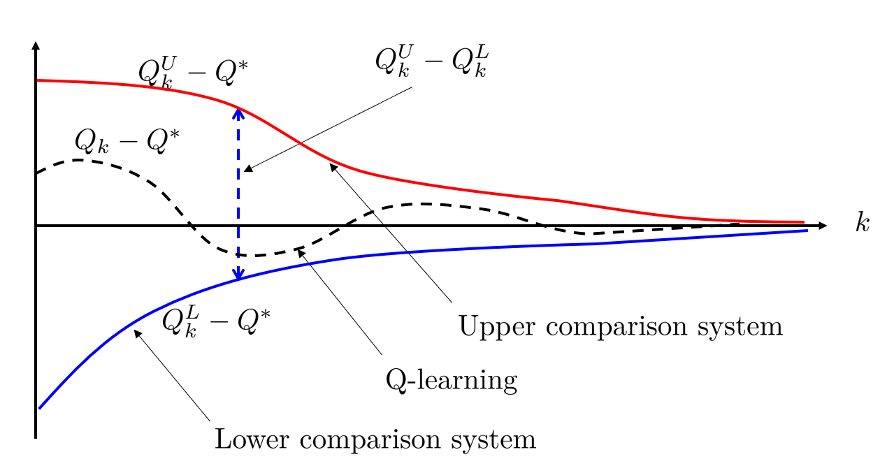
Proceeding on, consider the stochastic update (15). Ignoring the stochastic term $\alpha_{k}w_{k}$, it can be viewed as a discrete-time switched affine system. Unfortunately, analysis of a switched affine system is more involved than that of a switched linear system. The recent result in [31] overcame this difficulty by introducing the notion of the upper and lower comparison systems corresponding to the original system. In particular, [31] introduced a switching system representation of the continuous-time O.D.E. model corresponding to Q-learning. Then, the stability has been proved based on comparison of the upper and lower comparison systems of the original system in (15). Moreover, [33] extended this framework to a discrete-time setting, and derived finite-time convergence analysis under constant step-sizes. The overall idea is illustrated in Figure 1. However, when a time-varying step-size is used, it imposes significant difficulties in the analysis, which will be illustrated in the following sections.

Refer to caption
Figure 1: Upper and lower comparison systems

4 Analysis of lower comparison system

This section provides construction of a lower comparison system, and its finite time analysis. The construction of the lower comparison system follows that of [33]. With the help of a similarity transform, the convergence analysis follows the spirit of [39], which is a well-known approach to prove convergence rate in optimization literature.

4.1 Construction of lower comparison system

By the lower comparison system, we mean a dynamic system whose state at time $k$, denoted by $Q^{L}_{k}$, bounds the original system’s state $Q_{k}$ from below on the orthant, i.e., $Q^{L}_{k}\leq Q_{k}$. In particular, the lower comparison system can be expressed as follows:

Qk+1LQ=AQ,k(QkLQ)+αkwk.subscriptsuperscript𝑄𝐿𝑘1superscript𝑄subscript𝐴superscript𝑄𝑘subscriptsuperscript𝑄𝐿𝑘superscript𝑄subscript𝛼𝑘subscript𝑤𝑘\displaystyle Q^{L}_{k+1}-Q^{*}=A_{Q^{*},k}(Q^{L}_{k}-Q^{*})+\alpha_{k}w_{k}. (17)

Compared to the original system in (15), the main difference is the affine term $b_{Q_{k},k}$, which does not appear in the lower comparison system. For completeness, we provide the proof of the essential property, $Q^{L}_{k}\leq Q_{k}$, in the following lemma.

Lemma 4.1 ([33]).

When $Q^{L}_{0}-Q^{*}\leq Q_{0}-Q^{*}$,

QkLQQkQ.subscriptsuperscript𝑄𝐿𝑘superscript𝑄subscript𝑄𝑘superscript𝑄\displaystyle Q^{L}_{k}-Q^{*}\leq Q_{k}-Q^{*}. (18)
Proof.

The proof is done by induction. Assume for some $k\geq 0$, (18) satisfies. Now, we prove that the inequality is also satisfied for $(k+1)$-th iterate.

Qk+1LQsubscriptsuperscript𝑄𝐿𝑘1superscript𝑄\displaystyle Q^{L}_{k+1}-Q^{*} =AQ,k(QkLQ)+αkwkabsentsubscript𝐴superscript𝑄𝑘subscriptsuperscript𝑄𝐿𝑘superscript𝑄subscript𝛼𝑘subscript𝑤𝑘\displaystyle=A_{Q^{*},k}(Q^{L}_{k}-Q^{*})+\alpha_{k}w_{k}
$\displaystyle\leq A_{Q^{*},k}(Q_{k}-Q^{*})+\alpha_{k}w_{k}$
$\displaystyle=A_{Q_{k},k}(Q_{k}-Q^{*})-(A_{Q_{k},k}-A_{Q^{*},k})(Q_{k}-Q^{*})+\alpha_{k}w_{k}$
$\displaystyle=A_{Q_{k},k}(Q_{k}-Q^{*})+\alpha_{k}(\gamma DP\Pi_{Q^{*}}-\gamma DP\Pi_{Q_{k}})(Q_{k}-Q^{*})+\alpha_{k}w_{k}$
$\displaystyle\leq A_{Q_{k},k}(Q_{k}-Q^{*})+\alpha_{k}(\gamma DP\Pi_{Q_{k}}-\gamma DP\Pi_{Q^{*}})Q^{*}+\alpha_{k}w_{k}$
$\displaystyle=Q_{k+1}-Q^{*},$

where the first inequality is due to the hypothesis and the fact that $A_{Q,k}$ is positive matrix for any $Q$. Moreover, the second inequality can be driven using the fact that $\Pi_{Q^{*}}Q_{k}\leq\Pi_{Q_{k}}Q_{k}$ and $\Pi_{Q_{k}}Q^{*}\leq\Pi_{Q^{*}}Q^{*}$. ∎

To analyze the stochastic process generated by the lower comparison system, we define the notation $\mathcal{F}_{k}^{L}$ as follows:

  1. 1.

    $\mathcal{F}_{k}^{L}$ for i.i.d. observation: $\sigma$-field induced by $\{(s_{i},a_{i},s_{i}^{\prime},r_{i},Q_{i},Q^{L}_{i})\}_{i=0}^{k}$

  2. 2.

    $\mathcal{F}_{k}^{L}$ for Markovian observation: $\sigma$-field induced by $\{(s_{i},a_{i},s_{i+1},r_{i},Q_{i},Q^{L}_{i})\}_{i=0}^{k}$

4.2 Analysis of lower comparison system

This section provides a convergence rate of the lower comparison system. Let us consider the deterministic version of (17) as follows:

xk+1=AQ,kxk.subscript𝑥𝑘1subscript𝐴superscript𝑄𝑘subscript𝑥𝑘\displaystyle x_{k+1}=A_{Q^{*},k}x_{k}. (19)

The above system can be seen as a linear time-varying system. From Lemma 2.2, the existence of a positive definite matrix $P$ and a sequence $\{p_{k}\}$ such that $\Pi_{k=0}^{\infty}p_{k}\to 0$ ensures asymptotic stability of (19), when $P$ and $\{p_{k}\}$ satisfies below condition:

AQ,kPAQ,kpkPk0,formulae-sequenceprecedes-or-equalssubscriptsuperscript𝐴topsuperscript𝑄𝑘𝑃subscript𝐴superscript𝑄𝑘subscript𝑝𝑘𝑃for-all𝑘0\displaystyle A^{\top}_{Q^{*},k}PA_{Q^{*},k}\preceq p_{k}P\quad\forall{k}\geq 0, (20)

Here, $p_{k}$ can be controlled by an appropriate step-size. To proceed, let us choose $P=I$ to have

AQ,kPAQ,kpkP=((1pk)I+αk(TQ+TQ)+αk2TQTQ).subscriptsuperscript𝐴topsuperscript𝑄𝑘𝑃subscript𝐴superscript𝑄𝑘subscript𝑝𝑘𝑃1subscript𝑝𝑘𝐼subscript𝛼𝑘subscript𝑇superscript𝑄superscriptsubscript𝑇superscript𝑄topsuperscriptsubscript𝛼𝑘2subscriptsuperscript𝑇topsuperscript𝑄subscript𝑇superscript𝑄\displaystyle A^{\top}_{Q^{*},k}PA_{Q^{*},k}-p_{k}P=\left((1-p_{k})I+\alpha_{k}(T_{Q^{*}}+T_{Q^{*}}^{\top})+\alpha_{k}^{2}T^{\top}_{Q^{*}}T_{Q^{*}}\right). (21)

We want to find a step-size αksubscript𝛼𝑘\alpha_{k} such that the above equation is negative semidefinite. To this end, it is necessary that the second term TQ+TQsubscript𝑇superscript𝑄superscriptsubscript𝑇superscript𝑄topT_{Q^{*}}+T_{Q^{*}}^{\top} is negative definite. However, since TQ+TQsubscript𝑇superscript𝑄superscriptsubscript𝑇superscript𝑄topT_{Q^{*}}+T_{Q^{*}}^{\top} is not necessarily negative definite in general, it is hard to specify general conditions for a diminishing step-size to satisfy (20). To overcome this difficulty, we will consider the recent result in [30]. In particular, [30] studied convergence of linear stochastic recursions in Section 2.7, and a similarity transform was used in order to transform the matrix A𝐴A in (10) into a negative definite matrix. In this paper, we will apply a similar idea to derive the convergence rate of the lower comparison system. First of all, we will find a similarity transform of TQsubscript𝑇superscript𝑄T_{Q^{*}} to a negative definite matrix using the fact that TQsubscript𝑇superscript𝑄T_{Q^{*}} is Hurwitz. Then, the Lyapunov theory can be applied to derive the convergence results.

4.2.1 Similarity transformation to a negative definite matrix

In this subsection, we find a similarity transform of $T_{Q^{*}}$ to a negative definite matrix. Such a similarity transform has been used in estimation of an upper bound of the solution of Lyapunov equation in [18]. Moreover, in control community, a common similarity transform to an upper triangular matrix has been used to study a convergence rate of switched linear systems in [45]. Furthermore, [30] used a similarity transform based on the solution of Lyapunov equation to analyze stochastic approximation under a constant step-size without specification on the upper bound of the solution of a Lyapunov equation. However, in our case, we can derive the upper bound on the solution of the Lyapunov equation. First, let us consider the following continuous-time Lyapunov equation [11] for $T_{Q^{*}}$:

GTQ+TQG=I,𝐺subscript𝑇superscript𝑄superscriptsubscript𝑇superscript𝑄top𝐺𝐼GT_{Q^{*}}+T_{Q^{*}}^{\top}G=-I, (22)

where $G=G^{\top}\succ 0$ is called the Lyapunov matrix. If $T_{Q^{*}}$ is Hurwitz, then there exists a Lyapunov matrix $G$ such that the Lyapunov equation is satisfied, where $G$ is given by

G=0(eTQt)(eTQt)𝑑t.𝐺superscriptsubscript0superscriptsuperscript𝑒subscript𝑇superscript𝑄𝑡topsuperscript𝑒subscript𝑇superscript𝑄𝑡differential-d𝑡G=\int_{0}^{\infty}{(e^{T_{Q^{*}}t})^{\top}(e^{T_{Q^{*}}t})dt}. (23)

Before proceeding on, we summarize preliminary results on the properties of $G$. In particular, upper and lower bounds on the spectral norm of $G$ will play a central role in our analysis.

Lemma 4.2.
  1.  1)

    $||G||_{2}$ satisfies

    $\displaystyle\frac{1}{4(|\mathcal{S}|\mathcal{A}|)^{\frac{1}{2}}d_{\max}}\leq||G||_{2}\leq\frac{|\mathcal{S}||\mathcal{A}|}{2(1-\gamma)d_{\min}}.$
  2.  2)

    $||G^{-1}||_{2}$ satisfies

    $\displaystyle\frac{2(1-\gamma)d_{\min}}{|\mathcal{S}||\mathcal{A}|}\leq||G^{-1}||_{2}\leq 4(|\mathcal{S}||\mathcal{A}|)^{\frac{1}{2}}d_{\max}.$

The proof is given in Appendix Section 9.5. Now, let us consider a similarity transform of TQsubscript𝑇superscript𝑄T_{Q^{*}} using the Lyapunov matrix G𝐺G as follows:

B:=G1/2TQG1/2.assign𝐵superscript𝐺12subscript𝑇superscript𝑄superscript𝐺12B:=G^{1/2}T_{Q^{*}}G^{-1/2}. (24)

Then, we can prove that $B$ is negative definite, i.e., $\frac{B+B^{\top}}{2}\prec 0$. In particular, it can be proved using the following relations:

B+B𝐵superscript𝐵top\displaystyle B+B^{\top} =G1/2TQG1/2+G1/2TQG1/2=G1/2(GTQ+TQG)G1/2=G10.absentsuperscript𝐺12subscript𝑇superscript𝑄superscript𝐺12superscript𝐺12superscriptsubscript𝑇superscript𝑄topsuperscript𝐺12superscript𝐺12𝐺subscript𝑇superscript𝑄subscriptsuperscript𝑇topsuperscript𝑄𝐺superscript𝐺12superscript𝐺1precedes0\displaystyle=G^{1/2}T_{Q^{*}}G^{-1/2}+G^{-1/2}T_{Q^{*}}^{\top}G^{1/2}=G^{-1/2}(GT_{Q^{*}}+T^{\top}_{Q^{*}}G)G^{-1/2}=-G^{-1}\prec 0. (25)

In our main development, bounds on $B$ will play an important role as well.

Lemma 4.3.

$||B||_{2}$ satisfies

$\displaystyle\frac{(1-\gamma)d_{\min}}{|\mathcal{S}||\mathcal{A}|}\leq||B||_{2}\leq 2(|\mathcal{S}||\mathcal{A}|)^{\frac{5}{4}}d_{\max}.$

The proof is given in Appendix Section 9.6. Using the developed similarly transform from $T_{Q^{*}}$ to $B$ and changing the coordinate of the state in (17), we can construct another linear system which has more favorable structures. In particular, let us define the new state

zk:=G1/2(QkLQ).assignsubscript𝑧𝑘superscript𝐺12subscriptsuperscript𝑄𝐿𝑘𝑄z_{k}:=G^{1/2}(Q^{L}_{k}-Q). (26)

Then, the original lower comparison system in (17) can be transformed to

zk+1subscript𝑧𝑘1\displaystyle z_{k+1} =G1/2(Qk+1LQ)absentsuperscript𝐺12subscriptsuperscript𝑄𝐿𝑘1superscript𝑄\displaystyle=G^{1/2}(Q^{L}_{k+1}-Q^{*})
$\displaystyle=G^{1/2}(I+\alpha_{k}T_{Q^{*}})(Q^{L}_{k}-Q^{*})+\alpha_{k}G^{1/2}w_{k}$
$\displaystyle=G^{1/2}(I+\alpha_{k}T_{Q^{*}})G^{-1/2}z_{k}+\alpha_{k}G^{1/2}w_{k}$
$\displaystyle=(I+\alpha_{k}B)z_{k}+\alpha_{k}G^{1/2}w_{k},$

which corresponds to the new state $z_{k}$. To simplify expressions, let us introduce the notation

Xk:=I+αkB.assignsubscript𝑋𝑘𝐼subscript𝛼𝑘𝐵X_{k}:=I+\alpha_{k}B. (27)

Using this notation, the last equation can be rewritten as

zk+1=Xkzk+αkG1/2wk.subscript𝑧𝑘1subscript𝑋𝑘subscript𝑧𝑘subscript𝛼𝑘superscript𝐺12subscript𝑤𝑘\displaystyle z_{k+1}=X_{k}z_{k}+\alpha_{k}G^{1/2}w_{k}. (28)

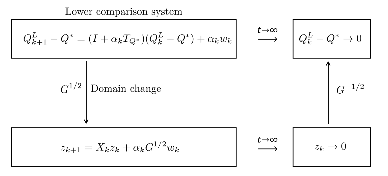
In this paper, we will analyze the convergence of $z_{k}$ instead of $Q^{L}_{k}-Q^{*}$. Then, it will ensure the convergence of the original state $Q^{L}_{k}-Q^{*}$. The main benefit of analyzing the system (28) comes from negative definiteness of $B$, which will be detailed later. The overall proof scheme is shown in Figure 2.

Refer to caption
Figure 2: Our proof scheme: domain transformation

4.2.2 Choice of step-size

In this subsection, we elaborate our motivation for the choice of the step-size $\alpha_{k}$. It is known that the diminishing step-size $\frac{1}{k}$ leads to sample complexity which polynomially depends on $\frac{1}{1-\gamma}$ [17]. In this paper, we consider the following diminishing step-size:

αk=θk+ξ,subscript𝛼𝑘𝜃𝑘𝜉\displaystyle\alpha_{k}=\frac{\theta}{k+\xi}, (29)

where $\theta>0$ and $\xi>0$ are tuning parameters to be determined. There are two conditions to be considered in the choice of the tuning parameters, which are summarized below.

  1. 1.

    The step-size should satisfy the Lyapunov inequality in (20).

  2. 2.

    The choice of step-size should lead to (fast) convergence of both lower and upper comparison system.

In this paper, the two conditions can be satisfied with the following choice of coefficients:

  1. 1.

    First of all, $\xi>0$ is selected such that

    8σmax2(B)ν28subscriptsuperscript𝜎2𝐵superscript𝜈2\displaystyle\frac{8\sigma^{2}_{\max}(B)}{\nu^{2}} ξ16σmax2(B)ν2,absent𝜉16subscriptsuperscript𝜎2𝐵superscript𝜈2\displaystyle\leq\xi\leq\frac{16\sigma^{2}_{\max}(B)}{\nu^{2}}, (30)

    where

    ν:=min{(1γ)dmin,λmin(G1)}.assign𝜈1𝛾subscript𝑑subscript𝜆superscript𝐺1\displaystyle\nu:=\min\{(1-\gamma)d_{\min},\lambda_{\min}(G^{-1})\}. (31)
  2. 2.

    Once $\xi>0$ is chosen based on the above rule, then $\theta$ can be selected as

    θ=ν2σmax2(B)ξ.𝜃𝜈2subscriptsuperscript𝜎2𝐵𝜉\displaystyle\theta=\frac{\nu}{2\sigma^{2}_{\max}(B)}\xi. (32)

Note that the upper bound on ξ𝜉\xi is chosen for simplicity of the proof. However, it can be arbitrarily large. With the above setup, we have the following results.

Lemma 4.4.

The following statements hold true:

  1. 1)

    Using the step-size in (29), we have

    λmax(XkXk)1βαk,subscript𝜆subscriptsuperscript𝑋top𝑘subscript𝑋𝑘1𝛽subscript𝛼𝑘\displaystyle\lambda_{\max}(X^{\top}_{k}X_{k})\leq 1-\beta\alpha_{k}, (33)

    where

    β:=σmax2(B)α0+ν=ν2>0.assign𝛽subscriptsuperscript𝜎2𝐵subscript𝛼0𝜈𝜈20\displaystyle\beta:=-\sigma^{2}_{\max}(B)\alpha_{0}+\nu=\frac{\nu}{2}>0. (34)
  2. 2)

    The conditions in (30) and (32) ensure

    βθ2,𝛽𝜃2\displaystyle\beta\theta\geq 2, (35)

    where $\beta$ is defined in (34), and

    dmin(1γ)θ2.subscript𝑑1𝛾𝜃2\displaystyle d_{\min}(1-\gamma)\theta\geq 2. (36)
Proof.

We first prove the first item. The upper bound of $\lambda_{\max}(I+\alpha_{k}(B+B^{\top})+\alpha_{k}^{2}B^{\top}B)$ can be derived from the relations

λmax(I+αk(B+B)+αk2BB)subscript𝜆𝐼subscript𝛼𝑘𝐵superscript𝐵topsuperscriptsubscript𝛼𝑘2superscript𝐵top𝐵\displaystyle\lambda_{\max}(I+\alpha_{k}(B+B^{\top})+\alpha_{k}^{2}B^{\top}B) =1+αkλmax((B+B)+αkBB))\displaystyle=1+\alpha_{k}\lambda_{\max}((B+B^{\top})+\alpha_{k}B^{\top}B))
$\displaystyle=1+\alpha_{k}\lambda_{\max}(-G^{-1}+\alpha_{k}B^{\top}B))$
$\displaystyle\leq 1+\alpha_{k}(\alpha_{k}\lambda_{\max}(B^{\top}B)-\lambda_{\min}(G^{-1}))$
$\displaystyle=1+\alpha_{k}(\sigma^{2}_{\max}(B)\alpha_{k}-\lambda_{\min}(G^{-1}))$
$\displaystyle\leq 1+\alpha_{k}(\sigma^{2}_{\max}(B)\alpha_{0}-\lambda_{\min}(G^{-1}))$
$\displaystyle\leq 1+\alpha_{k}(\sigma^{2}_{\max}(B)\alpha_{0}-\nu),$

where the first inequality follows from the fact that $G^{-1}$ and $B^{\top}B$ are positive definite, and the second inequality follows from the fact that $\alpha_{k}$ is a non-increasing sequence. The last inequality follows from the definition of $\nu$ defined in (31).

Next, we prove the second item. The proof can be readily done by the following simple algebraic inequalities:

$\displaystyle\beta\theta\geq\frac{\nu^{2}}{4\sigma^{2}_{\max}(B)}\xi\geq 2,$

and

$\displaystyle d_{\min}(1-\gamma)\theta\geq d_{\min}(1-\gamma)\frac{4}{\nu}\geq 2.$

This completes the proof. ∎

The first item in Lemma 4.4 implies that for the system in the new coordinate (28), the Lyapunov inequality in (20) is satisfied with $P=G$ and $p_{k}=1-\beta\alpha_{k}$ as follows:

AQ,kGAQ,ksubscriptsuperscript𝐴topsuperscript𝑄𝑘𝐺subscript𝐴superscript𝑄𝑘\displaystyle A^{\top}_{Q^{*},k}GA_{Q^{*},k} =G1/2G1/2(I+αkTQ)G(I+αkTQ)G1/2G1/2absentsuperscript𝐺12superscript𝐺12superscript𝐼subscript𝛼𝑘subscript𝑇superscript𝑄top𝐺𝐼subscript𝛼𝑘subscript𝑇superscript𝑄superscript𝐺12superscript𝐺12\displaystyle=G^{1/2}G^{-1/2}(I+\alpha_{k}T_{Q^{*}})^{\top}G(I+\alpha_{k}T_{Q^{*}})G^{-1/2}G^{1/2}
$\displaystyle=G^{1/2}(I+\alpha_{k}B)^{\top}(I+\alpha_{k}B)G^{1/2}$
$\displaystyle=G^{1/2}X_{k}^{\top}X_{k}G^{1/2}$
$\displaystyle\preceq(1-\beta\alpha_{k})G,$

where the second equality is due to the definition of $B$ in (24), and the last inequality follows from the first item of Lemma 4.4. Next, the second item shows that the choice of the diminishing step-size in (30) and (32) leads to fast convergence of both lower and upper comparison systems. To be more specific, $\beta$ and $d_{\min}(1-\gamma)$ are important factors in determining the convergence rate of lower and difference of upper and lower comparison systems, respectively. This can be seen as notions that are analogous to the strong convexity in [39]. As can been seen in the further analysis, intuitively, each Lyapunov function of the system can be thought of as decreasing by the factors of $\frac{\beta\theta}{k+\xi}$ and $\frac{d_{\min}(1-\gamma)\theta}{k+\xi}$ at $k$-th iteration. That is, denoting $V^{L}_{k}$ and $V^{U}_{k}$ a the Lyapunov functions of the upper and lower comparison systems at $k$-th iteration, we will have

Vk+1Lsubscriptsuperscript𝑉𝐿𝑘1\displaystyle V^{L}_{k+1} (1βθk+ξ)VkL+αkwkL,absent1𝛽𝜃𝑘𝜉superscriptsubscript𝑉𝑘𝐿subscript𝛼𝑘subscriptsuperscript𝑤𝐿𝑘\displaystyle\leq\left(1-\frac{\beta\theta}{k+\xi}\right)V_{k}^{L}+\alpha_{k}w^{L}_{k},
Vk+1Usubscriptsuperscript𝑉𝑈𝑘1\displaystyle V^{U}_{k+1} (1dmin(1γ)θk+ξ)VkU+αkwkU,absent1subscript𝑑1𝛾𝜃𝑘𝜉superscriptsubscript𝑉𝑘𝑈subscript𝛼𝑘subscriptsuperscript𝑤𝑈𝑘\displaystyle\leq\left(1-\frac{d_{\min}(1-\gamma)\theta}{k+\xi}\right)V_{k}^{U}+\alpha_{k}w^{U}_{k},

where $w^{L}_{k}$ and $w^{U}_{k}$ are bounded noise term for each system. If $\theta$ is small, the decreasing rate would be small, leading to slow convergence. Therefore, the step-size should be chosen to reflect these properties.

Remark 4.1.

Note that our choice of step-size can be expressed in terms of $d_{\min},|\cal{S}||\cal{A}|,$ and $1-\gamma$, since we can bound $\sigma^{2}_{\max}(B)$ from Lemma 4.3. However, in the sequel, we keep using $\sigma^{2}_{\max}(B)$ in the choice of step-sizes for convenience and simplicity of the proof.

4.2.3 Proof of convergence rate for lower comparison system

We now prove the convergence rate for (17), beginning with convergence rate for $z_{k}$. To this end, we will consider the simple quadratic Lyapunov function candidate

$\displaystyle V(z)=z^{\top}z,\quad z\in{\mathbb{R}}^{|{\cal S}||{\cal A}|}.$

Convergence of the Lyapunov function candidate is established in the sequel.

Proposition 4.1.

Consider the Lyapunov function candidate $V(z)=z^{\top}z$ in eq. 28. Under the step-size condition in (29), we have

$\displaystyle\mathbb{E}[V(z_{k})]\leq\frac{1}{k+\xi}\max\left\{\frac{8(|\mathcal{S}||\mathcal{A}|)^{\frac{11}{2}}d_{\max}^{2}}{(1-\gamma)^{3}d_{\min}^{3}}||Q^{L}_{0}-Q^{*}||^{2}_{2},\frac{72(|\mathcal{S}||\mathcal{A}|)^{3}}{(1-\gamma)^{5}d_{\min}^{3}}\right\}.$
Proof.

We first derive an upper bound on $\mathbb{E}[V(z_{k+1})|\mathcal{F}^{L}_{k}]$ from the relations

𝔼[V(zk+1)|kL]𝔼delimited-[]conditional𝑉subscript𝑧𝑘1subscriptsuperscript𝐿𝑘\displaystyle\mathbb{E}[V(z_{k+1})|\mathcal{F}^{L}_{k}] =𝔼[(zk)XkXk(zk)+2αkzkXkG1/2wk+αk2wkGwk|kL]absent𝔼delimited-[]superscriptsubscript𝑧𝑘topsuperscriptsubscript𝑋𝑘topsubscript𝑋𝑘subscript𝑧𝑘2subscript𝛼𝑘superscriptsubscript𝑧𝑘topsuperscriptsubscript𝑋𝑘topsuperscript𝐺12subscript𝑤𝑘conditionalsuperscriptsubscript𝛼𝑘2superscriptsubscript𝑤𝑘top𝐺subscript𝑤𝑘subscriptsuperscript𝐿𝑘\displaystyle=\mathbb{E}[(z_{k})^{\top}X_{k}^{\top}X_{k}(z_{k})+2\alpha_{k}z_{k}^{\top}X_{k}^{\top}G^{1/2}w_{k}+\alpha_{k}^{2}w_{k}^{\top}Gw_{k}|\mathcal{F}^{L}_{k}] (37)
$\displaystyle\leq(z_{k})^{\top}X_{k}^{\top}X_{k}(z_{k})+\alpha_{k}^{2}\lambda_{\max}(G)\frac{9}{(1-\gamma)^{2}}$
$\displaystyle\leq(1-\beta\alpha_{k})V(z_{k})+\alpha_{k}^{2}\lambda_{\max}(G)\frac{9}{(1-\gamma)^{2}}$
$\displaystyle=\left(1-\frac{\beta\theta}{k+\xi}\right)V(z_{k})+\frac{\theta^{2}}{(k+\xi)^{2}}\lambda_{\max}(G)\frac{9}{(1-\gamma)^{2}}$
$\displaystyle\leq\left(1-\frac{2}{k+\xi}\right)V(z_{k})+\frac{1}{(k+\xi)^{2}}\frac{16(|\mathcal{S}||\mathcal{A}|)^{2}}{(1-\gamma)^{2}d_{\min}^{2}}\frac{|\mathcal{S}||\mathcal{A}|}{2(1-\gamma)d_{\min}}\frac{9}{(1-\gamma)^{2}}$
$\displaystyle\leq\left(1-\frac{2}{k+\xi}\right)V(z_{k})+\frac{1}{(k+\xi)^{2}}\frac{72(|\mathcal{S}||\mathcal{A}|)^{3}}{(1-\gamma)^{5}d_{\min}^{3}},$

where $\mathcal{F}^{L}_{k}$ is defined as the $\sigma$-field induced by $\{(s_{i},a_{i},s_{i}^{\prime},r_{i},Q_{i},Q^{L}_{i})\}_{i=0}^{k}$. Here, the first inequality follows from

$$\mathbb{E}[2\alpha_{k}z_{k}^{\top}X_{k}^{\top}G^{1/2}w_{k}|\mathcal{F}^{L}_{k}]=0,$$

and the bound on $w_{k}$ given in (13). The second inequality comes from the bound given in Lemma 4.4. The third inequality is due to (35), and the last inequality is obtained simply by collecting the terms in the previous equations. Now, taking the total expectation, one gets

$\displaystyle\mathbb{E}[V(z_{k+1})]\leq\left(1-\frac{2}{k+\xi}\right)\mathbb{E}[V(z_{k})]+\frac{1}{(k+\xi)^{2}}\frac{72(|\mathcal{S}||\mathcal{A}|)^{3}}{(1-\gamma)^{5}d_{\min}^{3}}.$

To proceed further, an induction argument is applied. For simplicity, let us define the notation $\hat{k}:=k+\xi$, and suppose that

𝔼[V(zk)]1k^max{ξz022,72(|𝒮||𝒜|)3(1γ)5dmin3}𝔼delimited-[]𝑉subscript𝑧𝑘1^𝑘𝜉subscriptsuperscriptnormsubscript𝑧02272superscript𝒮𝒜3superscript1𝛾5superscriptsubscript𝑑3\displaystyle\mathbb{E}[V(z_{k})]\leq\frac{1}{\hat{k}}\max\left\{\xi||z_{0}||^{2}_{2},\frac{72(|\mathcal{S}||\mathcal{A}|)^{3}}{(1-\gamma)^{5}d_{\min}^{3}}\right\} (38)

holds. We now prove that $\mathbb{E}[V(z_{k+1})]\leq\frac{1}{\hat{k}+1}\max\left\{\xi||z_{0}||^{2}_{2},\frac{72(|\mathcal{S}||\mathcal{A}|)^{3}}{(1-\gamma)^{5}d_{\min}^{3}}\right\}$ holds. It is done by the inequalities

𝔼[V(zk+1)]𝔼delimited-[]𝑉subscript𝑧𝑘1\displaystyle\mathbb{E}[V(z_{k+1})] (12k^)1k^+1k^2max{ξz022,72(|𝒮||𝒜|)3(1γ)5dmin3}absent12^𝑘1^𝑘1superscript^𝑘2𝜉subscriptsuperscriptnormsubscript𝑧02272superscript𝒮𝒜3superscript1𝛾5superscriptsubscript𝑑3\displaystyle\leq\left(1-\frac{2}{\hat{k}}\right)\frac{1}{\hat{k}}+\frac{1}{\hat{k}^{2}}\max\left\{\xi||z_{0}||^{2}_{2},\frac{72(|\mathcal{S}||\mathcal{A}|)^{3}}{(1-\gamma)^{5}d_{\min}^{3}}\right\}
$\displaystyle\leq\left(\frac{1}{\hat{k}}-\frac{1}{\hat{k}^{2}}\right)\max\left\{\xi||z_{0}||^{2}_{2},\frac{72(|\mathcal{S}||\mathcal{A}|)^{3}}{(1-\gamma)^{5}d_{\min}^{3}}\right\}$
$\displaystyle\leq\frac{1}{\hat{k}+1}\max\left\{\xi||z_{0}||^{2}_{2},\frac{72(|\mathcal{S}||\mathcal{A}|)^{3}}{(1-\gamma)^{5}d_{\min}^{3}}\right\}.$

Hence, the inequality at k+1𝑘1k+1 is satisfied. Next, using Lemma 9.2 given in Appendix Section 9.2, we can bound ξz022𝜉superscriptsubscriptnormsubscript𝑧022\xi||z_{0}||_{2}^{2} as follows:

ξz022𝜉subscriptsuperscriptnormsubscript𝑧022\displaystyle\xi||z_{0}||^{2}_{2} 16(|𝒮||𝒜|)92dmax2(1γ)2dmin2G2Q0LQ22absent16superscript𝒮𝒜92superscriptsubscript𝑑2superscript1𝛾2superscriptsubscript𝑑2subscriptnorm𝐺2subscriptsuperscriptnormsubscriptsuperscript𝑄𝐿0superscript𝑄22\displaystyle\leq\frac{16(|\mathcal{S}||\mathcal{A}|)^{\frac{9}{2}}d_{\max}^{2}}{(1-\gamma)^{2}d_{\min}^{2}}||G||_{2}||Q^{L}_{0}-Q^{*}||^{2}_{2}
$\displaystyle\leq\frac{16(|\mathcal{S}||\mathcal{A}|)^{\frac{9}{2}}d_{\max}^{2}}{(1-\gamma)^{2}d_{\min}^{2}}\frac{|\mathcal{S}||\mathcal{A}|}{2(1-\gamma)d_{\min}}||Q^{L}_{0}-Q^{*}||^{2}_{2}$
$\displaystyle\leq\frac{8(|\mathcal{S}||\mathcal{A}|)^{\frac{11}{2}}d_{\max}^{2}}{(1-\gamma)^{3}d_{\min}^{3}}||Q^{L}_{0}-Q^{*}||^{2}_{2}.$

Applying above inequality to (38) and by the induction argument, we have

$\displaystyle\mathbb{E}[V(z_{k})]\leq\frac{1}{k+\xi}\max\left\{\frac{8(|\mathcal{S}||\mathcal{A}|)^{\frac{11}{2}}d_{\max}^{2}}{(1-\gamma)^{3}d_{\min}^{3}}||Q^{L}_{0}-Q^{*}||^{2}_{2},\frac{72(|\mathcal{S}||\mathcal{A}|)^{3}}{(1-\gamma)^{5}d_{\min}^{3}}\right\},$

which is the desired conclusion. ∎

Proposition 4.1 provides $\mathcal{O}(\frac{1}{k})$ convergence rate for ${\mathbb{E}}[V(z_{k})]={\mathbb{E}}[\left\|{z_{k}}\right\|_{2}^{2}]$ instead of ${\mathbb{E}}[V(Q_{k}^{L}-Q^{*})]={\mathbb{E}}[\left\|Q_{k}^{L}-Q^{*}\right\|_{2}^{2}]$. Since $Q_{k}^{L}-Q^{*}=G^{-1/2}(z_{k})$, it directly leads to the convergence rate corresponding to $Q_{k}^{L}-Q^{*}$, which can be derived with simple algebraic inequalities. The following theorem establishes its convergence rate.

Theorem 4.1.

Under the step-size (29), we have

$\displaystyle\mathbb{E}[||Q^{L}_{k}-Q^{*}||_{\infty}]\leq\frac{1}{\sqrt{k+\xi}}\max\left\{\frac{4(|\mathcal{S}||\mathcal{A}|)^{3}d_{\max}^{\frac{3}{2}}}{(1-\gamma)^{\frac{3}{2}}d_{\min}^{\frac{3}{2}}}||Q^{L}_{0}-Q^{*}||_{2},\frac{14(|\mathcal{S}||\mathcal{A}|)^{\frac{7}{4}}d_{\max}^{\frac{1}{2}}}{(1-\gamma)^{\frac{5}{2}}d_{\min}^{\frac{3}{2}}}\right\}.$
Proof.

Since $Q^{L}_{k}-Q^{*}=G^{-1/2}(z_{k})$, we have

𝔼[QkLQ22]𝔼delimited-[]subscriptsuperscriptnormsubscriptsuperscript𝑄𝐿𝑘superscript𝑄22\displaystyle\mathbb{E}[||Q^{L}_{k}-Q^{*}||^{2}_{2}] =𝔼[zkG1zk]absent𝔼delimited-[]subscriptsuperscript𝑧top𝑘superscript𝐺1subscript𝑧𝑘\displaystyle=\mathbb{E}[z^{\top}_{k}G^{-1}z_{k}]
$\displaystyle\leq\lambda_{\max}(G^{-1})\mathbb{E}[||z_{k}||^{2}_{2}]$
$\displaystyle\leq\frac{4(|\mathcal{S}||\mathcal{A}|)^{\frac{1}{2}}d_{\max}}{k+\xi}\max\left\{\frac{2(|\mathcal{S}||\mathcal{A}|)^{\frac{11}{2}}d_{\max}^{2}}{(1-\gamma)^{3}d_{\min}^{3}}||Q^{L}_{0}-Q^{*}||^{2}_{2},\frac{72(|\mathcal{S}||\mathcal{A}|)^{3}}{(1-\gamma)^{5}d_{\min}^{3}}\right\}$
$\displaystyle=\frac{1}{k+\xi}\max\left\{\frac{8(|\mathcal{S}||\mathcal{A}|)^{6}d_{\max}^{3}}{(1-\gamma)^{3}d_{\min}^{3}}||Q^{L}_{0}-Q^{*}||^{2}_{2},\frac{288(|\mathcal{S}||\mathcal{A}|)^{\frac{7}{2}}d_{\max}}{(1-\gamma)^{5}d_{\min}^{3}}\right\},$

where the first inequality is due to the positive definiteness of $G^{-1}$, and the second inequality follows from Proposition 4.1. Applying Jensen’s inequality to the above result yields

𝔼[QkLQ]𝔼delimited-[]subscriptnormsubscriptsuperscript𝑄𝐿𝑘superscript𝑄absent\displaystyle\mathbb{E}[||Q^{L}_{k}-Q^{*}||_{\infty}]\leq 𝔼[QkLQ2]𝔼delimited-[]subscriptnormsubscriptsuperscript𝑄𝐿𝑘superscript𝑄2\displaystyle\mathbb{E}[||Q^{L}_{k}-Q^{*}||_{2}]
\displaystyle\leq 𝔼[QkLQ22]𝔼delimited-[]subscriptsuperscriptnormsubscriptsuperscript𝑄𝐿𝑘superscript𝑄22\displaystyle\sqrt{\mathbb{E}[||Q^{L}_{k}-Q^{*}||^{2}_{2}]}
\displaystyle\leq 1k+ξmax{4(|𝒮||𝒜|)3dmax32(1γ)32dmin32Q0LQ2,14(|𝒮||𝒜|)74dmax12(1γ)52dmin32},1𝑘𝜉4superscript𝒮𝒜3superscriptsubscript𝑑32superscript1𝛾32superscriptsubscript𝑑32subscriptnormsubscriptsuperscript𝑄𝐿0superscript𝑄214superscript𝒮𝒜74superscriptsubscript𝑑12superscript1𝛾52superscriptsubscript𝑑32\displaystyle\frac{1}{\sqrt{k+\xi}}\max\left\{\frac{4(|\mathcal{S}||\mathcal{A}|)^{3}d_{\max}^{\frac{3}{2}}}{(1-\gamma)^{\frac{3}{2}}d_{\min}^{\frac{3}{2}}}||Q^{L}_{0}-Q^{*}||_{2},\frac{14(|\mathcal{S}||\mathcal{A}|)^{\frac{7}{4}}d_{\max}^{\frac{1}{2}}}{(1-\gamma)^{\frac{5}{2}}d_{\min}^{\frac{3}{2}}}\right\},

which is the desired conclusion. ∎

The convergence rate of lower comparison system depends on $(1-\gamma)^{-\frac{5}{2}}d_{\min}^{-\frac{3}{2}}$. As can be seen in the sequel, the upper comparison system has slower convergence rate then lower comparison system. The bottleneck of convergence rate of Q-learning may be due to the relatively slower convergence of the upper comparison system.

5 Upper comparison system

In this section, we focus on the construction of the upper comparison system. Then, its convergence analysis is discussed.

5.0.1 Construction of upper comparison system

As in [33], the upper comparison system in (15) can be derived as follows:

Qk+1UQ=AQk,k(QkUQ)+αkwk.subscriptsuperscript𝑄𝑈𝑘1superscript𝑄subscript𝐴subscript𝑄𝑘𝑘superscriptsubscript𝑄𝑘𝑈superscript𝑄subscript𝛼𝑘subscript𝑤𝑘\displaystyle~{}Q^{U}_{k+1}-Q^{*}=A_{Q_{k},k}(Q_{k}^{U}-Q^{*})+\alpha_{k}w_{k}. (39)

For completeness, we provide the proof that $Q^{U}_{k}$ upper bounds $Q_{k}$.

Lemma 5.1 ([33]).

If $Q^{U}_{0}-Q^{*}\geq Q_{0}-Q^{*}$, then

$\displaystyle Q^{U}_{k}-Q^{*}\geq Q_{k}-Q^{*}$

for all $k\geq 0$.

Proof.

The proof follows from induction. To this end, suppose that QkUQQkQsubscriptsuperscript𝑄𝑈𝑘superscript𝑄subscript𝑄𝑘superscript𝑄Q^{U}_{k}-Q^{*}\geq Q_{k}-Q^{*} holds for some k0𝑘0k\geq 0. Then, we have

Qk+1UQsubscriptsuperscript𝑄𝑈𝑘1superscript𝑄\displaystyle Q^{U}_{k+1}-Q^{*} =AQk,k(QkUQ)+αkwkabsentsubscript𝐴subscript𝑄𝑘𝑘superscriptsubscript𝑄𝑘𝑈superscript𝑄subscript𝛼𝑘subscript𝑤𝑘\displaystyle=A_{Q_{k},k}(Q_{k}^{U}-Q^{*})+\alpha_{k}w_{k}
$\displaystyle\geq A_{Q_{k},k}(Q_{k}^{U}-Q^{*})+b_{Q_{k},k}+\alpha_{k}w_{k}$
$\displaystyle\geq A_{Q_{k},k}(Q_{k}-Q^{*})+b_{Q_{k},k}+\alpha_{k}w_{k}$
$\displaystyle=Q_{k+1}-Q^{*},$

where the first inequality follows from the fact that $b_{Q_{k},k}\leq 0$. The second inequality is due to positiveness of $A_{Q_{k},k}$. This completes the proof. ∎

Since the upper comparison system in (39) is a switching linear system, it is not possible to obtain the corresponding convergence rate with the same techniques as in the lower comparison system. Moreover, we cannot find a common similarity transform matrix as in the lower comparison system case. Instead, we analyze the difference between $Q^{U}_{k}$ and $Q^{L}_{k}$ as in [33]. In particular, we consider the difference system

Qk+1UQk+1Lsubscriptsuperscript𝑄𝑈𝑘1subscriptsuperscript𝑄𝐿𝑘1\displaystyle Q^{U}_{k+1}-Q^{L}_{k+1} =AQk,k(QkUQLk)+BQk,k(QkLQ)absentsubscript𝐴subscript𝑄𝑘𝑘superscriptsubscript𝑄𝑘𝑈subscriptsuperscript𝑄𝑘𝐿subscript𝐵subscript𝑄𝑘𝑘subscriptsuperscript𝑄𝐿𝑘superscript𝑄\displaystyle=A_{Q_{k},k}(Q_{k}^{U}-Q^{k}_{L})+B_{Q_{k},k}(Q^{L}_{k}-Q^{*}) (40)

where

BQk,ksubscript𝐵subscript𝑄𝑘𝑘\displaystyle B_{Q_{k},k} :=AQk,kAQ,k=αkγDP(ΠQkΠQ).assignabsentsubscript𝐴subscript𝑄𝑘𝑘subscript𝐴superscript𝑄𝑘subscript𝛼𝑘𝛾𝐷𝑃subscriptΠsubscript𝑄𝑘subscriptΠsuperscript𝑄\displaystyle:=A_{Q_{k},k}-A_{Q^{*},k}=\alpha_{k}\gamma DP(\Pi_{Q_{k}}-\Pi_{Q^{*}}).

5.0.2 Proof of convergence rate for difference of upper and lower comparison systems

With the above setup, we are now ready to give the convergence rate of $\mathbb{E}[||Q^{U}_{k}-Q^{L}_{k}||_{\infty}]$. For simplicity of the proof, we assume $Q^{L}_{0}=Q^{U}_{0}$ without loss of generality.

Theorem 5.1.

Under the diminishing step-size in (29), we have

𝔼[QkUQkL]𝔼delimited-[]subscriptnormsubscriptsuperscript𝑄𝑈𝑘subscriptsuperscript𝑄𝐿𝑘\displaystyle\mathbb{E}[||Q^{U}_{k}-Q^{L}_{k}||_{\infty}] 1k+ξmax{16(|𝒮||𝒜|)4dmax52(1γ)52dmin52Q0LQ2,56(|𝒮||𝒜|)114dmax32(1γ)72dmin52}.absent1𝑘𝜉16superscript𝒮𝒜4superscriptsubscript𝑑52superscript1𝛾52superscriptsubscript𝑑52subscriptnormsubscriptsuperscript𝑄𝐿0superscript𝑄256superscript𝒮𝒜114superscriptsubscript𝑑32superscript1𝛾72superscriptsubscript𝑑52\displaystyle\leq\frac{1}{\sqrt{k+\xi}}\max\left\{\frac{16(|\mathcal{S}||\mathcal{A}|)^{4}d_{\max}^{\frac{5}{2}}}{(1-\gamma)^{\frac{5}{2}}d_{\min}^{\frac{5}{2}}}||Q^{L}_{0}-Q^{*}||_{2},\frac{56(|\mathcal{S}||\mathcal{A}|)^{\frac{11}{4}}d_{\max}^{\frac{3}{2}}}{(1-\gamma)^{\frac{7}{2}}d_{\min}^{\frac{5}{2}}}\right\}. (41)
Proof.

The proof follows similar lines as Theorem 4.1. We first take an expectation on the difference system (40), and use sub-multiplicativity of the norm as follows:

𝔼[Qk+1UQk+1L]𝔼delimited-[]subscriptnormsubscriptsuperscript𝑄𝑈𝑘1subscriptsuperscript𝑄𝐿𝑘1\displaystyle\mathbb{E}[||Q^{U}_{k+1}-Q^{L}_{k+1}||_{\infty}] 𝔼[AQk,kQkUQkL]+𝔼[BQkQkLQ]absent𝔼delimited-[]subscriptnormsubscript𝐴subscript𝑄𝑘𝑘subscriptnormsubscriptsuperscript𝑄𝑈𝑘subscriptsuperscript𝑄𝐿𝑘𝔼delimited-[]subscriptnormsubscript𝐵subscript𝑄𝑘subscriptnormsubscriptsuperscript𝑄𝐿𝑘superscript𝑄\displaystyle\leq\mathbb{E}[||A_{Q_{k},k}||_{\infty}||Q^{U}_{k}-Q^{L}_{k}||_{\infty}]+\mathbb{E}[||B_{Q_{k}}||_{\infty}||Q^{L}_{k}-Q^{*}||_{\infty}]
(1(1γ)dminαk)𝔼[QkUQkL]absent11𝛾subscript𝑑subscript𝛼𝑘𝔼delimited-[]subscriptnormsubscriptsuperscript𝑄𝑈𝑘subscriptsuperscript𝑄𝐿𝑘\displaystyle\leq\left(1-(1-\gamma)d_{\min}\alpha_{k}\right)\mathbb{E}[||Q^{U}_{k}-Q^{L}_{k}||_{\infty}] (42)
$\displaystyle+2\alpha_{k}\gamma d_{\max}\mathbb{E}[||Q^{L}_{k}-Q^{*}||_{\infty}]$
$\displaystyle\leq\left(1-\frac{2}{k+\xi}\right)\mathbb{E}[||Q^{U}_{k}-Q^{L}_{k}||_{\infty}]+\frac{2\theta\gamma d_{\max}}{k+\xi}\frac{C_{L}}{\sqrt{k+\xi}}$
$\displaystyle\leq\left(1-\frac{2}{k+\xi}\right)\mathbb{E}[||Q^{U}_{k}-Q^{L}_{k}||_{\infty}]+\frac{C_{U}}{(k+\xi)\sqrt{k+\xi}}$

where

CLsubscript𝐶𝐿\displaystyle C_{L} :=max{4(|𝒮||𝒜|)3dmax32(1γ)32dmin32Q0LQ2,14(|𝒮||𝒜|)74dmax12(1γ)52dmin32},assignabsent4superscript𝒮𝒜3superscriptsubscript𝑑32superscript1𝛾32superscriptsubscript𝑑32subscriptnormsubscriptsuperscript𝑄𝐿0superscript𝑄214superscript𝒮𝒜74superscriptsubscript𝑑12superscript1𝛾52superscriptsubscript𝑑32\displaystyle:=\max\left\{\frac{4(|\mathcal{S}||\mathcal{A}|)^{3}d_{\max}^{\frac{3}{2}}}{(1-\gamma)^{\frac{3}{2}}d_{\min}^{\frac{3}{2}}}||Q^{L}_{0}-Q^{*}||_{2},\frac{14(|\mathcal{S}||\mathcal{A}|)^{\frac{7}{4}}d_{\max}^{\frac{1}{2}}}{(1-\gamma)^{\frac{5}{2}}d_{\min}^{\frac{3}{2}}}\right\},
CUsubscript𝐶𝑈\displaystyle C_{U} :=max{16(|𝒮||𝒜|)4dmax52(1γ)52dmin52Q0LQ2,56(|𝒮||𝒜|)114dmax32(1γ)72dmin52}.assignabsent16superscript𝒮𝒜4superscriptsubscript𝑑52superscript1𝛾52superscriptsubscript𝑑52subscriptnormsubscriptsuperscript𝑄𝐿0superscript𝑄256superscript𝒮𝒜114superscriptsubscript𝑑32superscript1𝛾72superscriptsubscript𝑑52\displaystyle:=\max\left\{\frac{16(|\mathcal{S}||\mathcal{A}|)^{4}d_{\max}^{\frac{5}{2}}}{(1-\gamma)^{\frac{5}{2}}d_{\min}^{\frac{5}{2}}}||Q^{L}_{0}-Q^{*}||_{2},\frac{56(|\mathcal{S}||\mathcal{A}|)^{\frac{11}{4}}d_{\max}^{\frac{3}{2}}}{(1-\gamma)^{\frac{7}{2}}d_{\min}^{\frac{5}{2}}}\right\}.

The second inequality follows from Lemma 3.2, the third inequality is due to (36), and the last inequality comes from Lemma 9.2 given in Appendix Section 9.10. We proceed by induction. Let k^=k+ξ^𝑘𝑘𝜉\hat{k}=k+\xi, and suppose 𝔼[QkUQkL]CUk^𝔼delimited-[]subscriptnormsubscriptsuperscript𝑄𝑈𝑘subscriptsuperscript𝑄𝐿𝑘subscript𝐶𝑈^𝑘\mathbb{E}[||Q^{U}_{k}-Q^{L}_{k}||_{\infty}]\leq\frac{C_{U}}{\sqrt{\hat{k}}} for some k0𝑘0k\geq 0. Now, we prove that 𝔼[Qk+1UQk+1L]CUk^+1𝔼delimited-[]subscriptnormsubscriptsuperscript𝑄𝑈𝑘1subscriptsuperscript𝑄𝐿𝑘1subscript𝐶𝑈^𝑘1\mathbb{E}[||Q^{U}_{k+1}-Q^{L}_{k+1}||_{\infty}]\leq\frac{C_{U}}{\sqrt{\hat{k}+1}} holds as follows:

𝔼[Qk+1UQk+1L]𝔼delimited-[]subscriptnormsubscriptsuperscript𝑄𝑈𝑘1subscriptsuperscript𝑄𝐿𝑘1\displaystyle\mathbb{E}[||Q^{U}_{k+1}-Q^{L}_{k+1}||_{\infty}] CUk^2CUk^k^+CUk^k^absentsubscript𝐶𝑈^𝑘2subscript𝐶𝑈^𝑘^𝑘subscript𝐶𝑈^𝑘^𝑘\displaystyle\leq\frac{C_{U}}{\sqrt{\hat{k}}}-\frac{2C_{U}}{\hat{k}\sqrt{\hat{k}}}+\frac{C_{U}}{\hat{k}\sqrt{\hat{k}}}
$\displaystyle\leq\frac{C_{U}}{\sqrt{\hat{k}}}-\frac{C_{U}}{\hat{k}\sqrt{\hat{k}}}$
$\displaystyle\leq\frac{C_{U}}{\sqrt{\hat{k}+1}}.$

To prove the last inequality, we need to show 1k^1k^k^1k^+11^𝑘1^𝑘^𝑘1^𝑘1\frac{1}{\sqrt{\hat{k}}}-\frac{1}{\hat{k}\sqrt{\hat{k}}}\leq\frac{1}{\sqrt{\hat{k}+1}}. Multiplying k^32k^+1superscript^𝑘32^𝑘1\hat{k}^{\frac{3}{2}}\sqrt{\hat{k}+1} on both sides and rearranging the terms lead to (k^1)k^+1k^k^^𝑘1^𝑘1^𝑘^𝑘(\hat{k}-1)\sqrt{\hat{k}+1}\leq\hat{k}\sqrt{\hat{k}}. Now, it suffices to prove the last inequality. If 0<k^<10^𝑘10<\hat{k}<1, the inequality is trivial. When k^1^𝑘1\hat{k}\geq 1, taking square on both sides, we have

(k^22k^+1)(k^+1)superscript^𝑘22^𝑘1^𝑘1\displaystyle(\hat{k}^{2}-2\hat{k}+1)(\hat{k}+1) k^3.absentsuperscript^𝑘3\displaystyle\leq\hat{k}^{3}.

Rearranging the terms, the inequality becomes

2k^2+k^+k^22k^+12superscript^𝑘2^𝑘superscript^𝑘22^𝑘1\displaystyle-2\hat{k}^{2}+\hat{k}+\hat{k}^{2}-2\hat{k}+1 =k^2k^+10,absentsuperscript^𝑘2^𝑘10\displaystyle=-\hat{k}^{2}-\hat{k}+1\leq 0,

which proves the inequality $(\hat{k}-1)\sqrt{\hat{k}+1}\leq\hat{k}\sqrt{\hat{k}}$. This completes the proof. ∎

Compared to the convergence rate of the lower comparison system given in (17), the convergence rate for $Q^{U}_{k}-Q^{L}_{k}$ given in (40) depends on $(1-\gamma)^{-\frac{7}{2}}d_{\min}^{-\frac{5}{2}}$, which leads to slower convergence of the system.

6 Original system

With the bounds on upper and lower comparison systems, we are now ready to bound the original system in this section. We use simple algebraic inequalities to bound the original iterate ${\mathbb{E}}[||Q_{k}-Q^{*}||_{\infty}]$.

Theorem 6.1.

Under the step-size in (29), we have

$\displaystyle\mathbb{E}[||Q_{k}-Q^{*}||_{\infty}]\leq\frac{1}{\sqrt{k+\xi}}\max\left\{\frac{32(|\mathcal{S}||\mathcal{A}|)^{4}d_{\max}^{\frac{5}{2}}}{(1-\gamma)^{\frac{5}{2}}d_{\min}^{\frac{5}{2}}}||Q^{L}_{0}-Q^{*}||_{2},\frac{112(|\mathcal{S}||\mathcal{A}|)^{\frac{11}{4}}d_{\max}^{\frac{3}{2}}}{(1-\gamma)^{\frac{7}{2}}d_{\min}^{\frac{5}{2}}}\right\}.$
Proof.

The inequality follows from applying triangle inequality of the norm as follows:

𝔼[QkQ]𝔼delimited-[]subscriptnormsubscript𝑄𝑘superscript𝑄\displaystyle\mathbb{E}[||Q_{k}-Q^{*}||_{\infty}] 𝔼[QQkL]+𝔼[QkQkL]absent𝔼delimited-[]subscriptnormsuperscript𝑄subscriptsuperscript𝑄𝐿𝑘𝔼delimited-[]subscriptnormsubscript𝑄𝑘subscriptsuperscript𝑄𝐿𝑘\displaystyle\leq\mathbb{E}[||Q^{*}-Q^{L}_{k}||_{\infty}]+\mathbb{E}[||Q_{k}-Q^{L}_{k}||_{\infty}]
$\displaystyle\leq\mathbb{E}[||Q^{*}-Q^{L}_{k}||_{\infty}]+\mathbb{E}[||Q^{U}_{k}-Q^{L}_{k}||_{\infty}]$
$\displaystyle\leq\frac{1}{\sqrt{k+\xi}}\max\left\{\frac{4(|\mathcal{S}||\mathcal{A}|)^{3}d_{\max}^{\frac{3}{2}}}{(1-\gamma)^{\frac{3}{2}}d_{\min}^{\frac{3}{2}}}||Q^{L}_{0}-Q^{*}||_{2},\frac{14(|\mathcal{S}||\mathcal{A}|)^{\frac{7}{4}}d_{\max}^{\frac{1}{2}}}{(1-\gamma)^{\frac{5}{2}}d_{\min}^{\frac{3}{2}}}\right\}$
$\displaystyle+\frac{1}{\sqrt{k+\xi}}\max\left\{\frac{16(|\mathcal{S}||\mathcal{A}|)^{4}d_{\max}^{\frac{5}{2}}}{(1-\gamma)^{\frac{5}{2}}d_{\min}^{\frac{5}{2}}}||Q^{L}_{0}-Q^{*}||_{2},\frac{56(|\mathcal{S}||\mathcal{A}|)^{\frac{11}{4}}d_{\max}^{\frac{3}{2}}}{(1-\gamma)^{\frac{7}{2}}d_{\min}^{\frac{5}{2}}}\right\}$
$\displaystyle\leq\frac{1}{\sqrt{k+\xi}}\max\left\{\frac{32(|\mathcal{S}||\mathcal{A}|)^{4}d_{\max}^{\frac{5}{2}}}{(1-\gamma)^{\frac{5}{2}}d_{\min}^{\frac{5}{2}}}||Q^{L}_{0}-Q^{*}||_{2},\frac{112(|\mathcal{S}||\mathcal{A}|)^{\frac{11}{4}}d_{\max}^{\frac{3}{2}}}{(1-\gamma)^{\frac{7}{2}}d_{\min}^{\frac{5}{2}}}\right\},$

where the first inequality follows from triangle inequality. The second inequality is due to the fact that QkQkLQkUQkLsubscriptnormsubscript𝑄𝑘subscriptsuperscript𝑄𝐿𝑘subscriptnormsubscriptsuperscript𝑄𝑈𝑘subscriptsuperscript𝑄𝐿𝑘||Q_{k}-Q^{L}_{k}||_{\infty}\leq||Q^{U}_{k}-Q^{L}_{k}||_{\infty}. This is because 0QkQkLQkUQkL0subscript𝑄𝑘superscriptsubscript𝑄𝑘𝐿superscriptsubscript𝑄𝑘𝑈superscriptsubscript𝑄𝑘𝐿0\leq Q_{k}-Q_{k}^{L}\leq Q_{k}^{U}-Q_{k}^{L} holds. Moreover, the third inequality comes from Theorem 4.1 and Theorem 5.1. This completes the proof. ∎

Since $\mathbb{E}[||Q^{U}_{k}-Q^{L}_{k}]||_{\infty}]$ has a worse bound than $\mathbb{E}[||Q^{L}_{k}-Q^{*}||_{\infty}]$, convergence of $\mathbb{E}[||Q_{k}-Q^{*}||_{\infty}]$ is dominated by the bounds on $\mathbb{E}[||Q^{U}_{k}-Q^{L}_{k}]||_{\infty}]$.

7 Finite time analysis under Markovian noise

In the previous section, our analysis was based on i.i.d. observation model. However, in real-world scenarios, the state-action tuple follows Markovian observation model. In this section, we assume that the state-action pair follows a Markov chain as summarized in Section 2.6. The corresponding Q-learning algorithm with Markovian observation model in algorithm 2 can be written as follows:

Qk+1=Qk+αk(DR+γDPΠQkDQk+wk),subscript𝑄𝑘1subscript𝑄𝑘subscript𝛼𝑘subscript𝐷𝑅𝛾subscript𝐷𝑃subscriptΠsubscript𝑄𝑘subscript𝐷subscript𝑄𝑘subscript𝑤𝑘Q_{k+1}=Q_{k}+\alpha_{k}(D_{\infty}R+\gamma D_{\infty}P\Pi_{Q_{k}}-D_{\infty}Q_{k}+w_{k}), (43)

where $D_{\infty}\in{\mathbb{R}}^{|{\cal S}||{\cal A}|\times|{\cal S}||{\cal A}|}$ is a diagonal matrix with diagonal elements being the stationary state-action distributions, i.e.,

$\displaystyle(e_{s}\times e_{a})^{\top}D_{\infty}(e_{s}\times e_{a})=\mu_{\infty}(s,a)=\lim_{k\to\infty}{\mathbb{P}}[s_{k}=s,a_{k}=a|\beta],$

and

wksubscript𝑤𝑘\displaystyle w_{k} :=(eakesk)(eakesk)R+γ(eakesk)(esk+1)ΠQkQkassignabsenttensor-productsubscript𝑒subscript𝑎𝑘subscript𝑒subscript𝑠𝑘superscripttensor-productsubscript𝑒subscript𝑎𝑘subscript𝑒subscript𝑠𝑘top𝑅𝛾tensor-productsubscript𝑒subscript𝑎𝑘subscript𝑒subscript𝑠𝑘superscriptsubscript𝑒subscript𝑠𝑘1topsubscriptΠsubscript𝑄𝑘subscript𝑄𝑘\displaystyle:=(e_{a_{k}}\otimes e_{s_{k}})(e_{a_{k}}\otimes e_{s_{k}})^{\top}R+\gamma(e_{a_{k}}\otimes e_{s_{k}})(e_{s_{k+1}})^{\top}\Pi_{Q_{k}}Q_{k} (44)
$\displaystyle-(e_{a_{k}}\otimes e_{s_{k}})(e_{a_{k}}\otimes e_{s_{k}})^{\top}Q_{k}$
$\displaystyle-(D_{\infty}R+\gamma D_{\infty}P\Pi_{Q_{k}}Q_{k}-D_{\infty}Q_{k})$

is a noise term. Using the Bellman equation in (7), one can readily prove that the error term QkQsubscript𝑄𝑘superscript𝑄Q_{k}-Q^{*} evolves according to the following error dynamic system:

$\displaystyle Q_{k+1}-Q^{*}=A_{Q_{k},k}(Q_{k}-Q^{*})+b_{Q_{k},k}+\alpha_{k}w_{k},$

where

AQ,ksubscript𝐴𝑄𝑘\displaystyle A_{Q,k} :=I+αkTQbQ,k:=αkγDP(ΠQΠQ)Qformulae-sequenceassignabsent𝐼subscript𝛼𝑘subscript𝑇𝑄assignsubscript𝑏𝑄𝑘subscript𝛼𝑘𝛾subscript𝐷𝑃subscriptΠ𝑄subscriptΠsuperscript𝑄superscript𝑄\displaystyle:=I+\alpha_{k}T_{Q}\quad b_{Q,k}:=\alpha_{k}\gamma D_{\infty}P(\Pi_{Q}-\Pi_{Q^{*}})Q^{*} (45)
TQsubscript𝑇𝑄\displaystyle T_{Q} :=γDPΠQD.assignabsent𝛾subscript𝐷𝑃subscriptΠ𝑄subscript𝐷\displaystyle:=\gamma D_{\infty}P\Pi_{Q}-D_{\infty}.

Note that we can view $A_{Q,k}$ as a system matrix of a stochastic linear time-varying switching system as in the previous section. With slight abuse of notation, we use the notation $G$ for the solution of Lyapunov equation (22) with $T_{Q^{*}}$ in (45), and $B:=G^{1/2}T_{Q^{*}}G^{-1/2}$, the similarity transform of $T_{Q^{*}}$ to a negative definite matrix, and $X_{k}:=I+\alpha_{k}B$. $T_{Q^{*}}$ in (45) can be thought of as substituting $D$ in (16) with $D_{\infty}$. Since $G$, $B$, and $X_{k}$ only depend on $T_{Q^{*}}$, related lemmas still hold with $d_{\min}$ and $d_{\max}$ defined in Section 2.6 for the Markovian case. Moreover, due to the correlation of $Q_{k}$ and $(s_{k},a_{k},s_{k+1},r_{k})$, the noise term is biased, i.e., $\mathbb{E}[w_{k}|\mathcal{F}_{k}]\neq 0$, where $\mathcal{F}_{k}$ is defined as the $\sigma$-field induced by $\{(s_{i},a_{i},s_{i+1},r_{i},Q_{i})\}_{i=0}^{k}$. Therefore, the so-called crossing term in (37)

ξk(zk,Qk):=ξ(zk,Qk,ok):=zkXkG1/2wk(Qk).assignsubscript𝜉𝑘subscript𝑧𝑘subscript𝑄𝑘𝜉subscript𝑧𝑘subscript𝑄𝑘subscript𝑜𝑘assignsubscriptsuperscript𝑧top𝑘superscriptsubscript𝑋𝑘topsuperscript𝐺12subscript𝑤𝑘subscript𝑄𝑘\displaystyle\xi_{k}(z_{k},Q_{k}):=\xi(z_{k},Q_{k},o_{k}):=z^{\top}_{k}X_{k}^{\top}G^{1/2}w_{k}(Q_{k}). (46)

is not zero, where ok:=(sk,ak,rk+1,sk+1)assignsubscript𝑜𝑘subscript𝑠𝑘subscript𝑎𝑘subscript𝑟𝑘1subscript𝑠𝑘1o_{k}:=(s_{k},a_{k},r_{k+1},s_{k+1}) is the observation, which is the main difference compared to the analysis in the previous section. To resolve the difficulty, in this paper, we assume that the distribution μksubscript𝜇𝑘\mu_{k} mixes in a geometric rate to the stationary distribution μsubscript𝜇\mu_{\infty}, i.e., μkμsubscript𝜇𝑘subscript𝜇\mu_{k}\to\mu_{\infty} as k𝑘k\to\infty exponentially. Note that this assumption is standard and common in the literature [44, 7, 16, 12, 35], which study stochastic optimization algorithms with Markovian observation models. With the help of geometric mixing rate of the underlying Markov chain, our aim is to bound (46) by 𝒪(τmix(αk)k)𝒪superscript𝜏mixsubscript𝛼𝑘𝑘\mathcal{O}\left(\frac{\tau^{\text{mix}}(\alpha_{k})}{k}\right). The previous study in [7] has proved that such biased noise in standard TD-learning can be bounded by 𝒪(τmix(αk)k)𝒪superscript𝜏mixsubscript𝛼𝑘𝑘\mathcal{O}\left(\frac{\tau^{\text{mix}}(\alpha_{k})}{k}\right) with an additional projection step. In this paper, we prove that with our setups, we can easily follow the spirits of [7], and prove convergence of Q-learning without the additional projection step.

Finally, in this section, we separate the index of the observation $\{o_{k}\}_{k=1}^{n}$and the iterate $\{Q_{k}\}_{k=1}^{n}$ in the noise term, i.e.,

wj(Qi)subscript𝑤𝑗subscript𝑄𝑖\displaystyle w_{j}(Q_{i}) :=(eajesj)(eajesj)R+γ(eajesj)(esj+1)ΠQiQiassignabsenttensor-productsubscript𝑒subscript𝑎𝑗subscript𝑒subscript𝑠𝑗superscripttensor-productsubscript𝑒subscript𝑎𝑗subscript𝑒subscript𝑠𝑗top𝑅𝛾tensor-productsubscript𝑒subscript𝑎𝑗subscript𝑒subscript𝑠𝑗superscriptsubscript𝑒subscript𝑠𝑗1topsubscriptΠsubscript𝑄𝑖subscript𝑄𝑖\displaystyle:=(e_{a_{j}}\otimes e_{s_{j}})(e_{a_{j}}\otimes e_{s_{j}})^{\top}R+\gamma(e_{a_{j}}\otimes e_{s_{j}})(e_{s_{j+1}})^{\top}\Pi_{Q_{i}}Q_{i}
$\displaystyle-(e_{a_{j}}\otimes e_{s_{j}})(e_{a_{j}}\otimes e_{s_{j}})^{\top}Q_{i}$
$\displaystyle-(D_{\infty}R+\gamma D_{\infty}P\Pi_{Q_{i}}Q_{i}-D_{\infty}Q_{i}).$

Moreover, we will use the notation $w(o_{j},Q_{i}):=w_{j}(Q_{i})$ interchangeably in order to specify the dependence of the noise on the observation. The subscript of $w_{j}$ indicates the time index of observation, while the subscript of $Q_{i}$ is the time index corresponding to Q-iteration. When their indices coincide, that is, having both $k$-th observation of $\{o_{k}\}_{k=1}^{n}$ and $k$-the iterate of $\{Q_{k}\}_{k=1}^{n}$, we use $w_{k}$. Similar to the i.i.d. case, we can bound the noise term as follows:

Lemma 7.1.

Under Markovian observation model in (44), the stochastic noise can be bounded as follows:

wksubscriptnormsubscript𝑤𝑘\displaystyle||w_{k}||_{\infty} 41γ,absent41𝛾\displaystyle\leq\frac{4}{1-\gamma},
𝔼[wk22k]𝔼delimited-[]conditionalsubscriptsuperscriptnormsubscript𝑤𝑘22subscript𝑘\displaystyle\mathbb{E}[||w_{k}||^{2}_{2}\mid\mathcal{F}_{k}] 16|𝒮||𝒜|(1γ)2,absent16𝒮𝒜superscript1𝛾2\displaystyle\leq\frac{16|\mathcal{S}||\mathcal{A}|}{(1-\gamma)^{2}},

where $\mathcal{F}_{k}$ is the $\sigma$-field induced by $\{(s_{i},a_{i},s_{i+1},r_{i},Q_{i})\}_{i=0}^{k}$.

The proof is in Appendix Section 9.7.

7.1 Preliminaries on information theoretic results

In this subsection, we introduce some definitions used in information theory, and its relation to the Markov chain under our consideration.

Definition 7.1 (Total variation distance [34]).

The total variation distance between two probability distributions $P$ and $Q$ on the sample space, $\Omega$, is defined as

$\displaystyle d_{\text{TV}}(P,Q):=\max_{A\in\Omega}|P(A)-Q(A)|.$
Definition 7.2 (Conditional independence [28]).

For random variables X,Y, and Z,

$\displaystyle X\to Y\to Z$

denotes that $X$ and $Z$ are conditionally independent given $Y$, that is, ${\mathbb{P}}(Z|X,Y)={\mathbb{P}}(Z|Y)$.

Throughout the analysis, we will consider standard assumptions on Markov chain. With 2.1, the Markov chain reaches its stationary distribution at a geometric rate. We note that most of the analysis of stochastic optimization on Markov chain [44, 7, 16, 12, 35] relies on geometric convergence to the stationary distribution. Our analysis also adopts this standard scenario.

Lemma 7.2 ([34]).

Under 2.1, there exist constants $m>0$ and $\rho\in(0,1)$ such that

$$d_{\text{TV}}(\mu_{k},\mu_{\infty})\leq m\rho^{k},\quad\forall{k}\in\mathbb{N},$$

where $\mu_{k}$ and $\mu_{\infty}$ are defined in (9).

Now, we can define the mixing-time as follows:

τmix(c):=min{kmρkc},assignsuperscript𝜏mix𝑐𝑘conditional𝑚superscript𝜌𝑘𝑐\displaystyle\tau^{\text{mix}}(c):=\min\{k\in\mathbb{N}\mid m\rho^{k}\leq c\}, (47)

which is the minimum time required for the total variation distance between the stationary distribution and the current distribution to be less than a desired level $c>0$. Moreover, $m$ and $\rho$ are the constants defined in Lemma 7.2.

Related to the mixing-time, let us introduce the following quantity:

Kmix:=min{kt2τmix(αt),tk},assignsubscript𝐾mixconditional𝑘𝑡2superscript𝜏mixsubscript𝛼𝑡for-all𝑡𝑘\displaystyle K_{\text{mix}}:=\min\{k\mid t\geq 2\tau^{\text{mix}}(\alpha_{t}),\forall{t\geq k}\}, (48)

where $\alpha_{t}$ is the step-size defined in (29). Note that $K_{\text{mix}}$ is well-defined, since upper bound of $\tau^{\text{mix}}(\alpha_{k})$ is logarithmically proportional to $k$. Intuitively, $K_{\text{mix}}$ roughly means the number of iterations, after which the mixing-time corresponding to the current step-size can be upper bounded by the current time. Therefore, the analysis can be divided into two phases, the first phase $k\leq K_{\text{mix}}$ and the second phase $k\geq K_{\text{mix}}$. Note that this approach is common in the literature. For example, the recent paper [12] derived a convergence rate after some quantity similar to $K_{\text{mix}}$ iterations, and [35] derived a sample complexity after some time related to the mixing time. For $k\leq K_{\text{mix}}$ , we can ensure the iterate remains bounded, and after $k\geq K_{\text{mix}}$, we have $\mathcal{O}\left(\sqrt{\frac{\tau^{\text{mix}}(\alpha_{k})}{k}}\right)$ convergence rate. Lastly, we state a key lemma to prove a bound on (46) with $\mathcal{O}\left(\frac{\tau^{\text{mix}}(\alpha_{k})}{k}\right)$.

Lemma 7.3 (Control of coupling [7]).

For some $k\geq 0$, and $\tau>0$, consider two random variables $X$ and $Y$ such that

$$X\to(s_{k},a_{k})\to(s_{k+\tau},a_{k+\tau})\to Y.$$

Let the underlying Markov chain, {(sk,ak)}k=0superscriptsubscriptsubscript𝑠𝑘subscript𝑎𝑘𝑘0\{(s_{k},a_{k})\}_{k=0}^{\infty}, satisfies 2.1. Moreover, let us construct independent random variables Xsuperscript𝑋X^{\prime} and Ysuperscript𝑌Y^{\prime} drawn from the marginal distributions of X𝑋X and Y𝑌Y, respectively, i.e., X(X=)similar-tosuperscript𝑋𝑋X^{\prime}\sim\mathbb{P}(X=\cdot) and Y(Y=)similar-tosuperscript𝑌𝑌Y^{\prime}\sim\mathbb{P}(Y=\cdot) so that

$\displaystyle\mathbb{P}(X^{\prime}=\cdot,Y^{\prime}=\cdot)=\mathbb{P}(X^{\prime}=\cdot)\mathbb{P}(Y^{\prime}=\cdot)=\mathbb{P}(X=\cdot)\mathbb{P}(Y=\cdot).$

Then, for any function $f:\mathcal{X}\times\mathcal{Y}\to\mathbb{R}$ such that $\sup_{(x,y)\in\mathcal{X}\times\mathcal{Y}}|f(x,y)|<\infty$, we have

$$|\mathbb{E}[f(X,Y)]-\mathbb{E}[f(X^{\prime},Y^{\prime})]|\leq 2\sup_{(x,y)\in\mathcal{X}\times\mathcal{Y}}|f(x,y)|(m\rho^{\tau}).$$

7.2 Bounding the crossing term $\mathbb{E}[\xi_{k}(z_{k},Q_{k})]$

With our assumptions in place, we are now ready to bound the crossing term, 𝔼[ξk(zk,Qk)]𝔼delimited-[]subscript𝜉𝑘subscript𝑧𝑘subscript𝑄𝑘\mathbb{E}[\xi_{k}(z_{k},Q_{k})], provided that the iterate zksubscript𝑧𝑘z_{k} is bounded, which is required because the crossing term is a function of Markovian noise and zksubscript𝑧𝑘z_{k}. In this subsection, we also need to establish the boundedness of QkLQsubscriptsuperscript𝑄𝐿𝑘superscript𝑄Q^{L}_{k}-Q^{*}. As in 2.2, we assume that Q0L1subscriptnormsubscriptsuperscript𝑄𝐿01||Q^{L}_{0}||_{\infty}\leq 1. Note that it is always possible because Q01subscriptnormsubscript𝑄01||Q_{0}||_{\infty}\leq 1, and we can always set Q0=Q0Lsubscript𝑄0subscriptsuperscript𝑄𝐿0Q_{0}=Q^{L}_{0} without loss of generality.

Lemma 7.4 (Boundedness of $Q^{L}_{k}-Q^{*}$ and $z_{k}$).

Suppose that $||Q^{L}_{0}||_{\infty}\leq 1$ holds. Then, the following statements hold true:

  1. 1)

    For all k0𝑘0k\geq 0, we have

    $\displaystyle||Q_{k}^{L}-Q^{*}||_{\infty}\leq\frac{4}{(1-\gamma)^{2}d_{\min}}.$
  2. 2)

    From item 1), for all $k\geq 0$ we have,

    $\displaystyle||z_{k}||_{\infty}\leq\frac{8(|\mathcal{S}||\mathcal{A}|)^{\frac{1}{2}}}{(1-\gamma)^{\frac{5}{2}}d_{\min}^{\frac{3}{2}}}.$
Proof.

We first prove the boundedness of QkLQsuperscriptsubscript𝑄𝑘𝐿superscript𝑄Q_{k}^{L}-Q^{*} by an induction argument. For k=0𝑘0k=0, we have

$$||Q^{L}_{0}-Q^{*}||_{\infty}\leq\frac{4}{(1-\gamma)^{2}d_{\min}},$$

because

Q0LQsubscriptnormsubscriptsuperscript𝑄𝐿0superscript𝑄\displaystyle||Q^{L}_{0}-Q^{*}||_{\infty} Q0L+Qabsentsubscriptnormsubscriptsuperscript𝑄𝐿0subscriptnormsuperscript𝑄\displaystyle\leq||Q^{L}_{0}||_{\infty}+||Q^{*}||_{\infty}
$\displaystyle\leq 1+\frac{1}{1-\gamma}$
$\displaystyle=\frac{2-\gamma}{1-\gamma}\leq\frac{4}{(1-\gamma)^{2}d_{\min}},$

where the last inequality follows from Lemma 2.3. Next, suppose that $||Q^{L}_{k}-Q^{*}||_{\infty}\leq\frac{4}{(1-\gamma)^{2}d_{\min}}$ holds for some $k\geq 0$. Then, we have

Qk+1LQsubscriptnormsubscriptsuperscript𝑄𝐿𝑘1superscript𝑄\displaystyle||Q^{L}_{k+1}-Q^{*}||_{\infty} AQ,kQkLQ+αkwkabsentsubscriptnormsubscript𝐴superscript𝑄𝑘subscriptnormsubscriptsuperscript𝑄𝐿𝑘superscript𝑄subscript𝛼𝑘subscriptnormsubscript𝑤𝑘\displaystyle\leq||A_{Q^{*},k}||_{\infty}||Q^{L}_{k}-Q^{*}||_{\infty}+\alpha_{k}||w_{k}||_{\infty}
$\displaystyle\leq(1-d_{\min}(1-\gamma)\alpha_{k})||Q^{L}_{k}-Q^{*}||_{\infty}+\alpha_{k}\frac{4}{1-\gamma}$
$\displaystyle\leq\frac{4}{(1-\gamma)^{2}d_{\min}},$

where the first inequality follows from the update of lower comparison system (17), and the second inequality comes from the bound on wksubscript𝑤𝑘w_{k} in Lemma 7.1 and AQ,ksubscript𝐴superscript𝑄𝑘A_{Q^{*},k} in Lemma 3.2. Then, the proof is completed by induction. Next, the boundedness of zksubscript𝑧𝑘z_{k} naturally follows from the coordinate transform in (28). In particular, it follows from the inequalities

zksubscriptnormsubscript𝑧𝑘\displaystyle||z_{k}||_{\infty} G1/2QkLQ8(|𝒮||𝒜|)12(1γ)52dmin32,absentsubscriptnormsuperscript𝐺12subscriptnormsubscriptsuperscript𝑄𝐿𝑘superscript𝑄8superscript𝒮𝒜12superscript1𝛾52superscriptsubscript𝑑32\displaystyle\leq||G^{1/2}||_{\infty}||Q^{L}_{k}-Q^{*}||_{\infty}\leq\frac{8(|\mathcal{S}||\mathcal{A}|)^{\frac{1}{2}}}{(1-\gamma)^{\frac{5}{2}}d_{\min}^{\frac{3}{2}}},

where the second inequality follows from Lemma 4.2 to bound $||G^{1/2}||_{\infty}$. This completes the proof. ∎

With the boundedness of $z_{k}$, we can bound the crossing term as follows.

Lemma 7.5 (Bound on $\xi_{k}(z_{k},Q_{k})$ and Lipschitzness).
  1. 1)

    The crossing term $\xi_{k}(z_{k},Q_{k})$ at $k$-th iterate is always bounded as follows:

    $\displaystyle|\xi_{k}(z_{k},Q_{k})|\leq\frac{32(||\mathcal{S}||\mathcal{A}|)^{3}}{(1-\gamma)^{4}d_{\min}^{2}}.$
  2. 2)

    For any $k\geq 0$, $\xi_{k}(z,Q)$ is Lipschitz with respect to $(z,Q)$, i.e.,

    $\displaystyle|\xi_{k}(z,Q)-\xi_{k}(z^{\prime},Q^{\prime})|\leq\frac{16(|\mathcal{S}||\mathcal{A}|)^{3}}{(1-\gamma)^{3}d_{\min}^{2}}||Q-Q^{\prime}||_{\infty}+\frac{4(|\mathcal{S}||\mathcal{A}|)^{\frac{3}{2}}}{(1-\gamma)^{\frac{3}{2}}d_{\min}^{\frac{1}{2}}}||z-z^{\prime}||_{\infty}$

The proof is given in Appendix Section 9.8. Using above results, we are now in position to provide a bound on the crossing term, $\mathbb{E}[\xi_{k}(z_{k},Q_{k})]$. Before proceeding further, we will first obtain a bound on the delayed term, $\mathbb{E}[\xi_{k}(z_{k-\tau},Q_{k-\tau})]$, and then derive a bound of the crossing term, $\mathbb{E}[\xi_{k}(z_{k},Q_{k})]$.

Lemma 7.6 (Boundedness of $\mathbb{E}[\xi_{k}(z_{k-\tau},Q_{k-\tau})]$ ).

For any $\tau$ and $k$ such that $0\leq\tau\leq k$, there exist $m>0$ anr $0<\rho<1$ such that

𝔼[ξk(zkτ,Qkτ)]𝔼delimited-[]subscript𝜉𝑘subscript𝑧𝑘𝜏subscript𝑄𝑘𝜏\displaystyle\mathbb{E}[\xi_{k}(z_{k-\tau},Q_{k-\tau})] 96(|𝒮||𝒜|)3(1γ)4dmin2(mρτ).absent96superscript𝒮𝒜3superscript1𝛾4superscriptsubscript𝑑2𝑚superscript𝜌𝜏\displaystyle\leq\frac{96(|\mathcal{S}||\mathcal{A}|)^{3}}{(1-\gamma)^{4}d_{\min}^{2}}(m\rho^{\tau}).
Proof.

Using some simple decomposition, we can get

$\displaystyle|{\mathbb{E}}[\xi_{k}(z_{k-\tau},Q_{k-\tau})]|$
$\displaystyle=|{\mathbb{E}}[\xi_{k}(z_{k-\tau},Q_{k-\tau})]-{\mathbb{E}}[\xi(z_{k-\tau}^{\prime},Q_{k-\tau}^{\prime},o_{k}^{\prime})]+{\mathbb{E}}[\xi(z_{k-\tau}^{\prime},Q_{k-\tau}^{\prime},o_{k}^{\prime})]|$
|𝔼[ξ(zkτ,Qkτ,ok)]𝔼[ξ(zkτ,Qkτ,ok)]|+|𝔼[ξ(zkτ,Qkτ,ok)]|,absent𝔼delimited-[]𝜉subscript𝑧𝑘𝜏subscript𝑄𝑘𝜏subscript𝑜𝑘𝔼delimited-[]𝜉superscriptsubscript𝑧𝑘𝜏superscriptsubscript𝑄𝑘𝜏superscriptsubscript𝑜𝑘𝔼delimited-[]𝜉superscriptsubscript𝑧𝑘𝜏superscriptsubscript𝑄𝑘𝜏superscriptsubscript𝑜𝑘\displaystyle\leq|{\mathbb{E}}[\xi(z_{k-\tau},Q_{k-\tau},o_{k})]-{\mathbb{E}}[\xi(z_{k-\tau}^{\prime},Q_{k-\tau}^{\prime},o_{k}^{\prime})]|+|{\mathbb{E}}[\xi(z_{k-\tau}^{\prime},Q_{k-\tau}^{\prime},o_{k}^{\prime})]|, (49)

where the first inequality is due to triangle inequality. The first term in the above inequality can be bounded with the coupling lemma in Lemma 7.3, and the second term can be bounded with the help of independent coupling construction and ergodic assumption in 2.1.

First, we will bound $|{\mathbb{E}}[\xi(z_{k-\tau},Q_{k-\tau},o_{k})]-{\mathbb{E}}[\xi(z_{k-\tau}^{\prime},Q_{k-\tau}^{\prime},o_{k}^{\prime})]|$ in (49). To apply Lemma 7.3, first note the relations

$\displaystyle(z_{k-\tau},Q_{k-\tau})\to(s_{k-\tau},a_{k-\tau})\to(s_{k},a_{k})\to o_{k},$

where the arrow notation is defined in Definition 7.2, and $o_{k}:=(s_{k},a_{k},r_{k+1},s_{k+1})$. Now, let us construct the coupling distribution of $(z_{k-\tau}^{\prime},Q_{k-\tau}^{\prime})$ and $o^{\prime}_{k}$ drawn independently from some marginal distributions of $(z_{k-\tau},Q_{k-\tau})$ and $o_{k}$, respectively, i.e., $(z_{k-\tau}^{\prime},Q_{k-\tau}^{\prime})\sim{\mathbb{P}}((z_{k-\tau},Q_{k-\tau})=\cdot)$ and $o_{k}^{\prime}\sim{\mathbb{P}}(o_{k}=\cdot)$. From the fact that $\xi_{k}$ is bounded, which is given in the first statement of Lemma 7.5, we can now apply Lemma 7.3, leading to

|𝔼[ξ(zkτ,Qkτ,ok)]𝔼[ξ(zkτ,Qkτ,ok)]|64(|𝒮||𝒜|)3(1γ)4dmin2mρτ.𝔼delimited-[]𝜉subscript𝑧𝑘𝜏subscript𝑄𝑘𝜏subscript𝑜𝑘𝔼delimited-[]𝜉superscriptsubscript𝑧𝑘𝜏subscriptsuperscript𝑄𝑘𝜏superscriptsubscript𝑜𝑘64superscript𝒮𝒜3superscript1𝛾4superscriptsubscript𝑑2𝑚superscript𝜌𝜏\displaystyle|{\mathbb{E}}[\xi(z_{k-\tau},Q_{k-\tau},o_{k})]-{\mathbb{E}}[\xi(z_{k-\tau}^{\prime},Q^{\prime}_{k-\tau},o_{k}^{\prime})]|\leq\frac{64(|\mathcal{S}||\mathcal{A}|)^{3}}{(1-\gamma)^{4}d_{\min}^{2}}m\rho^{\tau}. (50)

Next, we will bound |𝔼[ξ(zkτ,Qkτ,ok)]|𝔼delimited-[]𝜉subscriptsuperscript𝑧𝑘𝜏subscriptsuperscript𝑄𝑘𝜏subscriptsuperscript𝑜𝑘|\mathbb{E}[\xi(z^{\prime}_{k-\tau},Q^{\prime}_{k-\tau},o^{\prime}_{k})]| in (49) from the construction of coupling that (zkτ,Qkτ)subscriptsuperscript𝑧𝑘𝜏subscriptsuperscript𝑄𝑘𝜏(z^{\prime}_{k-\tau},Q^{\prime}_{k-\tau}) and oksubscriptsuperscript𝑜𝑘o^{\prime}_{k} are independent, and ergodic assumption from 2.1. Using the tower property of expectation, i.e., 𝔼[X]=𝔼[𝔼[X|Y]]𝔼delimited-[]𝑋𝔼delimited-[]𝔼delimited-[]conditional𝑋𝑌\mathbb{E}[X]=\mathbb{E}[\mathbb{E}[X|Y]], convexity of |||\cdot|, and Jensen’s inequality, we have

|𝔼[ξ(zkτ,Qkτ,ok))]|\displaystyle|\mathbb{E}[\xi(z^{\prime}_{k-\tau},Q^{\prime}_{k-\tau},o^{\prime}_{k}))]| =|𝔼[𝔼[ξ(zkτ,Qkτ,ok)|zkτ,Qkτ]]|\displaystyle=|\mathbb{E}[\mathbb{E}[\xi(z^{\prime}_{k-\tau},Q^{\prime}_{k-\tau},o^{\prime}_{k})|z_{k-\tau}^{\prime},Q_{k-\tau}^{\prime}]]|
𝔼[|𝔼[ξ(zkτ,Qkτ,ok)|zkτ,Qkτ]|].\displaystyle\leq\mathbb{E}[|\mathbb{E}[\xi(z^{\prime}_{k-\tau},Q^{\prime}_{k-\tau},o^{\prime}_{k})|z_{k-\tau}^{\prime},Q_{k-\tau}^{\prime}]|]. (51)

Now, our aim is to bound $|\mathbb{E}[\xi(z^{\prime}_{k-\tau},Q^{\prime}_{k-\tau},o^{\prime}_{k})|z_{k-\tau}^{\prime},Q_{k-\tau}^{\prime}]|$ in the last inequality. Denoting the noise term in (44) with the observation $o^{\prime}_{k}$ as $w_{k}^{\prime}(Q_{k-\tau}^{\prime})$, we first bound the noise term. Let us define $D_{\mu_{k}}$ to denote the state-action distribution at $k$-th time step as follows:

$\displaystyle(e_{s}\times e_{a})^{\top}D_{\mu_{k}}(e_{s}\times e_{a})=\mu_{k}(s,a)={\mathbb{P}}[s_{k}=s,a_{k}=a|\beta],$

where $\mu_{k}$ is defined in (8). The noise term $w_{k}^{\prime}(Q_{k-\tau}^{\prime})$ defined in (44) can be bounded as follows:

||𝔼[wk(Qkτ)|zkτ,Qkτ]||\displaystyle||\mathbb{E}[w_{k}^{\prime}(Q_{k-\tau}^{\prime})|z_{k-\tau}^{\prime},Q_{k-\tau}^{\prime}]||_{\infty} DμkDR+γPΠQkτQkτQkτabsentsubscriptnormsubscript𝐷subscript𝜇𝑘subscript𝐷subscriptnorm𝑅𝛾𝑃subscriptΠsubscript𝑄𝑘𝜏subscript𝑄𝑘𝜏subscript𝑄𝑘𝜏\displaystyle\leq||D_{\mu_{k}}-D_{\infty}||_{\infty}||R+\gamma P\Pi_{Q_{k-\tau}}Q_{k-\tau}-Q_{k-\tau}||_{\infty}
$\displaystyle\leq\frac{2}{1-\gamma}||D_{\mu_{k}}-D_{\infty}||_{\infty}$
$\displaystyle=\frac{2}{1-\gamma}\max_{(s,a)\in\mathcal{S}\times\mathcal{A}}|\mu_{k}(s,a)-\mu_{\infty}(s,a)|$
$\displaystyle=\frac{2}{1-\gamma}d_{\text{TV}}(\mu_{k},\mu_{\infty})$
21γmρk,absent21𝛾𝑚superscript𝜌𝑘\displaystyle\leq\frac{2}{1-\gamma}m\rho^{k}, (52)

where the first inequality follows from the fact that $o^{\prime}_{k}$ is independent with $Q^{\prime}_{k-\tau}$, and the second inequality follows from 2.2 and Lemma 2.3. In particular, the first equality comes from the definition of the infinity norm, and the second equality follows from definition of the total variation distance in Definition 7.1. The last inequality follows from the ergodicity assumption of the Markov chain in Lemma 7.2.

With the above result, we can now bound $|\mathbb{E}[\xi(z^{\prime}_{k-\tau},Q^{\prime}_{k-\tau},o^{\prime}_{k})|z_{k-\tau}^{\prime},Q_{k-\tau}^{\prime}]|$ as follows:

|𝔼[ξ(zkτ,Qkτ,ok)\displaystyle|\mathbb{E}[\xi(z^{\prime}_{k-\tau},Q^{\prime}_{k-\tau},o^{\prime}_{k}) |zkτ,Qkτ]|\displaystyle|z_{k-\tau}^{\prime},Q_{k-\tau}^{\prime}]|
$\displaystyle=|z_{k-\tau}^{\top\prime}X_{k}^{\top}G^{1/2}\mathbb{E}[w^{\prime}_{k}(Q^{\prime}_{k-\tau})|z_{k-\tau}^{\prime},Q_{k-\tau}^{\prime}]|$
$\displaystyle\leq|\mathcal{S}||\mathcal{A}|||X_{k}z_{k-\tau}^{\prime}||_{2}||G^{1/2}||_{2}||\mathbb{E}[w^{\prime}_{k}(Q^{\prime}_{k-\tau})|z_{k-\tau}^{\prime},Q_{k-\tau}^{\prime}]||_{\infty}$
$\displaystyle\leq\frac{16(|\mathcal{S}||\mathcal{A}|)^{3}}{(1-\gamma)^{4}d_{\min}^{2}}||\mathbb{E}[w_{k}^{\prime}(Q_{k-\tau}^{\prime})|z_{k-\tau}^{\prime},Q_{k-\tau}^{\prime}]||_{\infty}$
$\displaystyle\leq\frac{32(|\mathcal{S}||\mathcal{A}|)^{3}}{(1-\gamma)^{4}d_{\min}^{2}}m\rho^{k},$

where the first equality is due to the definition of the crossing term in (46). The first inequality is due to Hölder’s inequality, and the second inequality follows from Lemma 7.4 and Lemma 4.2. Applying (52), we obtain the last inequality. Combining the above result with (51) leads to

|𝔼[ξ(zkτ,Qkτ,ok))]|32(|𝒮||𝒜|)3(1γ)4dmin2mρk.\displaystyle|\mathbb{E}[\xi(z^{\prime}_{k-\tau},Q^{\prime}_{k-\tau},o^{\prime}_{k}))]|\leq\frac{32(|\mathcal{S}||\mathcal{A}|)^{3}}{(1-\gamma)^{4}d_{\min}^{2}}m\rho^{k}. (53)

Now, we are ready to finish the proof. Bounding each term in (49) with (50) and (53), we have

$\displaystyle|{\mathbb{E}}[\xi_{k}(z_{k-\tau},Q_{k-\tau})]|\leq\frac{96(|\mathcal{S}||\mathcal{A}|)^{3}}{(1-\gamma)^{4}d_{\min}^{2}}m\rho^{\tau}.$

This completes the proof. ∎

The above lemma states that if $\tau$, the time difference between the new observation $o_{k}$ and previous iterate $Q_{k-\tau}$, is large, then the Markovian noise term $w(o_{k},Q_{k-\tau})$ inherits the geometric mixing property of the Markov chain. Now, combining the above result with Lipschitzness of $\xi_{k}(z_{k},Q_{k})$, we can bound the crossing term, $\mathbb{E}[\xi_{k}(z_{k},Q_{k})]$, as follows.

Lemma 7.7 (Boundedness of $\mathbb{E}[\xi_{k}(z_{k},Q_{k})]$ ).

For $k\geq K_{\text{mix}}$, expectation of the cross term can be bounded as follows:

𝔼[ξk(zk,Qk)]𝔼delimited-[]subscript𝜉𝑘subscript𝑧𝑘subscript𝑄𝑘\displaystyle\mathbb{E}[\xi_{k}(z_{k},Q_{k})] (96(|𝒮||𝒜|)3(1γ)4dmin2+64(|𝒮||𝒜|)134(1γ)4dmin2τmix(αk))αkτmix(αk).absent96superscript𝒮𝒜3superscript1𝛾4superscriptsubscript𝑑264superscript𝒮𝒜134superscript1𝛾4superscriptsubscript𝑑2superscript𝜏mixsubscript𝛼𝑘subscript𝛼𝑘superscript𝜏mixsubscript𝛼𝑘\displaystyle\leq\left(\frac{96(|\mathcal{S}||\mathcal{A}|)^{3}}{(1-\gamma)^{4}d_{\min}^{2}}+\frac{64(|\mathcal{S}||\mathcal{A}|)^{\frac{13}{4}}}{(1-\gamma)^{4}d_{\min}^{2}}\tau^{\text{mix}}(\alpha_{k})\right)\alpha_{k-\tau^{\text{mix}}(\alpha_{k})}.
Proof.

From Lipschitzness of $\xi_{k}(z_{k},Q_{k})$ in Lemma 7.5, we have

ξk(zk,Qk)ξk(zkτ,Qkτ)subscript𝜉𝑘subscript𝑧𝑘subscript𝑄𝑘subscript𝜉𝑘subscript𝑧𝑘𝜏subscript𝑄𝑘𝜏\displaystyle\xi_{k}(z_{k},Q_{k})-\xi_{k}(z_{k-\tau},Q_{k-\tau}) |ξk(zk,Qk)ξk(zkτ,Qkτ)|absentsubscript𝜉𝑘subscript𝑧𝑘subscript𝑄𝑘subscript𝜉𝑘subscript𝑧𝑘𝜏subscript𝑄𝑘𝜏\displaystyle\leq|\xi_{k}(z_{k},Q_{k})-\xi_{k}(z_{k-\tau},Q_{k-\tau})|
$\displaystyle\leq\frac{16(|\mathcal{S}||\mathcal{A}|)^{3}}{(1-\gamma)^{3}d_{\min}^{2}}||Q_{k}-Q_{k-\tau}||_{\infty}$
+2(|𝒮||𝒜|)32(1γ)52dmin12zkzkτ.2superscript𝒮𝒜32superscript1𝛾52superscriptsubscript𝑑12subscriptnormsubscript𝑧𝑘subscript𝑧𝑘𝜏\displaystyle+\frac{2(|\mathcal{S}||\mathcal{A}|)^{\frac{3}{2}}}{(1-\gamma)^{\frac{5}{2}}d_{\min}^{\frac{1}{2}}}||z_{k}-z_{k-\tau}||_{\infty}. (54)

In the sequel, $||Q_{k}-Q_{k-\tau}||_{\infty}$ and $||z_{k}-z_{k-\tau}||_{\infty}$ will be bounded in terms of step-size. From the update of $z_{i}$ in (28), for $i\geq 0$, we have

zi+1zisubscriptnormsubscript𝑧𝑖1subscript𝑧𝑖\displaystyle||z_{i+1}-z_{i}||_{\infty} =αiBzi+αiG1/2wiabsentsubscriptnormsubscript𝛼𝑖𝐵subscript𝑧𝑖subscript𝛼𝑖superscript𝐺12subscript𝑤𝑖\displaystyle=||\alpha_{i}Bz_{i}+\alpha_{i}G^{1/2}w_{i}||_{\infty}
$\displaystyle\leq(||B||_{\infty}||z_{i}||_{\infty}+||G^{1/2}||_{\infty}||w_{i}||_{\infty})\alpha_{i}$
$\displaystyle\leq\left(||B||_{2}||z_{i}||_{\infty}+||G^{1/2}||_{2}\frac{4}{1-\gamma}\right)\alpha_{i}$
$\displaystyle\leq\left((1-\gamma)d_{\min}(|\mathcal{S}||\mathcal{A}|)^{\frac{5}{4}}\frac{8(|\mathcal{S}||\mathcal{A}|)^{\frac{1}{2}}}{(1-\gamma)^{\frac{5}{2}}d_{\min}^{\frac{3}{2}}}+\sqrt{\frac{|\mathcal{S}||\mathcal{A}|}{2(1-\gamma)d_{\min}}}\frac{4}{1-\gamma}\right)\alpha_{i}$
16(|𝒮||𝒜|)74(1γ)32dmin12αi,absent16superscript𝒮𝒜74superscript1𝛾32superscriptsubscript𝑑12subscript𝛼𝑖\displaystyle\leq\frac{16(|\mathcal{S}||\mathcal{A}|)^{\frac{7}{4}}}{(1-\gamma)^{\frac{3}{2}}d_{\min}^{\frac{1}{2}}}\alpha_{i}, (55)

where the second inequality follows from bounding wisubscript𝑤𝑖w_{i} in Lemma 7.1, and the third inequality is obtained by bounding each terms with Lemma 4.3 and Lemma 7.4. Similarly for Qisubscript𝑄𝑖Q_{i}, we have

Qi+1Qisubscriptnormsubscript𝑄𝑖1subscript𝑄𝑖\displaystyle||Q_{i+1}-Q_{i}||_{\infty} =αi||(eakesk)(eakesk)R+γ(eakesk)(esk+1)ΠQkQk\displaystyle=\alpha_{i}||(e_{a_{k}}\otimes e_{s_{k}})(e_{a_{k}}\otimes e_{s_{k}})^{\top}R+\gamma(e_{a_{k}}\otimes e_{s_{k}})(e_{s_{k+1}})^{\top}\Pi_{Q_{k}}Q_{k}
$\displaystyle-(e_{a_{k}}\otimes e_{s_{k}})(e_{a_{k}}\otimes e_{s_{k}})^{\top}Q_{k}||_{\infty}$
2γ1γαi.absent2𝛾1𝛾subscript𝛼𝑖\displaystyle\leq\frac{2-\gamma}{1-\gamma}\alpha_{i}. (56)

For any $k\geq 1$ and $\tau$ such that $1\leq\tau\leq k$, summing up (55) and (56) from $i=k-\tau$ to $k-1$, respectively, we get

zkzkτsubscriptnormsubscript𝑧𝑘subscript𝑧𝑘𝜏\displaystyle||z_{k}-z_{k-\tau}||_{\infty} i=kτk1zi+1zi16(|𝒮||𝒜|)74(1γ)32dmin12i=kτk1αi16(|𝒮||𝒜|)74(1γ)32dmin12ταkτ.absentsubscriptsuperscript𝑘1𝑖𝑘𝜏subscriptnormsubscript𝑧𝑖1subscript𝑧𝑖16superscript𝒮𝒜74superscript1𝛾32superscriptsubscript𝑑12subscriptsuperscript𝑘1𝑖𝑘𝜏subscript𝛼𝑖16superscript𝒮𝒜74superscript1𝛾32superscriptsubscript𝑑12𝜏subscript𝛼𝑘𝜏\displaystyle\leq\sum^{k-1}_{i=k-\tau}||z_{i+1}-z_{i}||_{\infty}\leq\frac{16(|\mathcal{S}||\mathcal{A}|)^{\frac{7}{4}}}{(1-\gamma)^{\frac{3}{2}}d_{\min}^{\frac{1}{2}}}\sum^{k-1}_{i=k-\tau}\alpha_{i}\leq\frac{16(|\mathcal{S}||\mathcal{A}|)^{\frac{7}{4}}}{(1-\gamma)^{\frac{3}{2}}d_{\min}^{\frac{1}{2}}}\tau\alpha_{k-\tau}.

The first inequality follows from triangle inequality. The second inequality follows from (55). The last inequality follows from the fact that $\alpha_{k}$ is decreasing sequence. Similarly, using (56), we have

QkQkτsubscriptnormsubscript𝑄𝑘subscript𝑄𝑘𝜏\displaystyle||Q_{k}-Q_{k-\tau}||_{\infty} i=kτk1Qi+1Qi2γ1γi=kτk1αi2γ1γταkτ.absentsubscriptsuperscript𝑘1𝑖𝑘𝜏subscriptnormsubscript𝑄𝑖1subscript𝑄𝑖2𝛾1𝛾subscriptsuperscript𝑘1𝑖𝑘𝜏subscript𝛼𝑖2𝛾1𝛾𝜏subscript𝛼𝑘𝜏\displaystyle\leq\sum^{k-1}_{i=k-\tau}||Q_{i+1}-Q_{i}||_{\infty}\leq\frac{2-\gamma}{1-\gamma}\sum^{k-1}_{i=k-\tau}\alpha_{i}\leq\frac{2-\gamma}{1-\gamma}\tau\alpha_{k-\tau}.

Therefore, combining the above results with (54) leads to

ξk(zk,Qk)ξk(zkτ,Qkτ)subscript𝜉𝑘subscript𝑧𝑘subscript𝑄𝑘subscript𝜉𝑘subscript𝑧𝑘𝜏subscript𝑄𝑘𝜏\displaystyle\xi_{k}(z_{k},Q_{k})-\xi_{k}(z_{k-\tau},Q_{k-\tau}) 32(|𝒮||𝒜|)3(1γ)4dmin2ταkτ+4(|𝒮||𝒜|)134(1γ)4dminταkτabsent32superscript𝒮𝒜3superscript1𝛾4superscriptsubscript𝑑2𝜏subscript𝛼𝑘𝜏4superscript𝒮𝒜134superscript1𝛾4subscript𝑑𝜏subscript𝛼𝑘𝜏\displaystyle\leq\frac{32(|\mathcal{S}||\mathcal{A}|)^{3}}{(1-\gamma)^{4}d_{\min}^{2}}\tau\alpha_{k-\tau}+\frac{4(|\mathcal{S}||\mathcal{A}|)^{\frac{13}{4}}}{(1-\gamma)^{4}d_{\min}}\tau\alpha_{k-\tau}
64(|𝒮||𝒜|)134(1γ)4dmin2ταkτ.absent64superscript𝒮𝒜134superscript1𝛾4superscriptsubscript𝑑2𝜏subscript𝛼𝑘𝜏\displaystyle\leq\frac{64(|\mathcal{S}||\mathcal{A}|)^{\frac{13}{4}}}{(1-\gamma)^{4}d_{\min}^{2}}\tau\alpha_{k-\tau}. (57)

Next, we will bound $\mathbb{E}[\xi_{k}(z_{k},Q_{k})]$. In particular, taking total expectations on (7.2) yields

$\displaystyle\mathbb{E}[\xi_{k}(z_{k},Q_{k})]\leq\mathbb{E}[\xi_{k}(z_{k-\tau},Q_{k-\tau})]+\frac{64(|\mathcal{S}||\mathcal{A}|)^{\frac{13}{4}}}{(1-\gamma)^{4}d_{\min}^{2}}\tau\alpha_{k-\tau}.$

Since the above inequality is satisfied for any $1\leq\tau\leq k$, for $k\geq K_{\text{mix}}$, we can set $\tau=\tau^{\text{mix}}(\alpha_{k})$ from the definition of $\tau^{\text{mix}}(\alpha_{k})$. Now, we have

𝔼[ξk(zk,Qk)]𝔼delimited-[]subscript𝜉𝑘subscript𝑧𝑘subscript𝑄𝑘\displaystyle\mathbb{E}[\xi_{k}(z_{k},Q_{k})] 96(|𝒮||𝒜|)3(1γ)4dmin2(mρτmix(αk))+64(|𝒮||𝒜|)134(1γ)4dmin2τmix(αk)αkτmix(αk)absent96superscript𝒮𝒜3superscript1𝛾4superscriptsubscript𝑑2𝑚superscript𝜌superscript𝜏mixsubscript𝛼𝑘64superscript𝒮𝒜134superscript1𝛾4superscriptsubscript𝑑2superscript𝜏mixsubscript𝛼𝑘subscript𝛼𝑘superscript𝜏mixsubscript𝛼𝑘\displaystyle\leq\frac{96(|\mathcal{S}||\mathcal{A}|)^{3}}{(1-\gamma)^{4}d_{\min}^{2}}(m\rho^{\tau^{\text{mix}}(\alpha_{k})})+\frac{64(|\mathcal{S}||\mathcal{A}|)^{\frac{13}{4}}}{(1-\gamma)^{4}d_{\min}^{2}}\tau^{\text{mix}}(\alpha_{k})\alpha_{k-\tau^{\text{mix}}(\alpha_{k})}
$\displaystyle\leq\frac{96(|\mathcal{S}||\mathcal{A}|)^{3}}{(1-\gamma)^{4}d_{\min}^{2}}\alpha_{k}+\frac{64(|\mathcal{S}||\mathcal{A}|)^{\frac{13}{4}}}{(1-\gamma)^{4}d_{\min}^{2}}\tau^{\text{mix}}(\alpha_{k})\alpha_{k-\tau^{\text{mix}}(\alpha_{k})}$
$\displaystyle\leq\left(\frac{96(|\mathcal{S}||\mathcal{A}|)^{3}}{(1-\gamma)^{4}d_{\min}^{2}}+\frac{64(|\mathcal{S}||\mathcal{A}|)^{\frac{13}{4}}}{(1-\gamma)^{4}d_{\min}^{2}}\tau^{\text{mix}}(\alpha_{k})\right)\alpha_{k-\tau^{\text{mix}}(\alpha_{k})},$

where the first inequality follows from Lemma 7.6, the second inequality comes from the definition of mixing time in (47), and the last inequality follows from the fact that $\alpha_{k}$ is a decreasing sequence. ∎

7.3 Finite time analysis under Markovian noise

Now, we turn to the statement of our main results. The proof logic follows similar arguments as in the i.i.d. setting with few modifications. First, we begin the overall proof by deriving the convergence rate of $z_{k}$, which corresponds to the lower comparison system with a coordinate transformation. Then, as a next step, we will consider the difference system to obtain a convergence rate of the original system. In the sequel, a generic constant $C>0$ will be used for unimportant values that change line by line.

Proposition 7.1 (Convergence rate of $z_{k}$).

Consider the step-size in (29) and Markovian observation model. For any $k\geq K_{\text{mix}}$, we have

$\displaystyle\mathbb{E}[V(z_{k})]\leq\frac{C_{2}}{k+\xi}+\frac{C(|\mathcal{S}||\mathcal{A}|)^{\frac{21}{4}}}{(1-\gamma)^{6}d_{\min}^{4}}\frac{\tau^{\text{mix}}(\alpha_{k})}{k+\xi},$

where $V(x)=x^{\top}x$ and $C_{2}:=C\max\left\{\frac{(|\mathcal{S}||\mathcal{A}|)^{\frac{11}{2}}d_{\max}^{2}}{(1-\gamma)^{3}d_{\min}^{3}}||Q^{L}_{0}-Q^{*}||^{2}_{2},\frac{(|\mathcal{S}||\mathcal{A}|)^{5}}{(1-\gamma)^{6}d_{\min}^{4}}\right\}$.

Proof.

We will follow similar lines as in the proof of Proposition 4.1. For simplicity of the induction proof, let $C_{1}:=\max\left\{\frac{8(|\mathcal{S}||\mathcal{A}|)^{\frac{11}{2}}d_{\max}^{2}}{(1-\gamma)^{3}d_{\min}^{3}}||Q^{L}_{0}-Q^{*}||^{2}_{2},\frac{72(|\mathcal{S}||\mathcal{A}|)^{4}}{(1-\gamma)^{5}d_{\min}^{3}}\right\}$. Plugging the term $z_{k+1}=X_{k}z_{k}+\alpha_{k}G^{1/2}w_{k}$ into $V(z_{k+1})$, we have the following relation:

$\displaystyle\mathbb{E}[V(z_{k+1})|\mathcal{F}^{L}_{k}]$
$\displaystyle=\mathbb{E}[(z_{k})^{\top}X_{k}^{\top}X_{k}(z_{k})+2\alpha_{k}z_{k}^{\top}X_{k}^{\top}G^{1/2}w_{k}+\alpha_{k}^{2}w_{k}^{\top}Gw_{k}|\mathcal{F}^{L}_{k}]$
$\displaystyle\leq(1-\beta\alpha_{k})\mathbb{E}[V(z_{k})]+2\alpha_{k}\mathbb{E}[\xi_{k}(z_{k},Q_{k})\mid\mathcal{F}^{L}_{k}]+\lambda_{\max}(G)\frac{\theta^{2}}{(k+\xi)^{2}}\mathbb{E}[||w_{k}||^{2}_{2}\mid\mathcal{F}_{k}^{L}]$
$\displaystyle\leq\left(1-\frac{2}{k+\xi}\right)\mathbb{E}[V(z_{k})]+\frac{C_{1}}{(k+\xi)^{2}}+2\alpha_{k}\mathbb{E}[\xi_{k}(z_{k},Q_{k})\mid\mathcal{F}_{k}^{L}],$

where $\mathcal{F}^{L}_{k}$ is a $\sigma$-field induced by $\{(s_{i},a_{i},s_{i+1},r_{i},Q_{i},Q_{i}^{L})\}_{i=0}^{k}$, the first inequality follows from bound on $||X_{k}||_{2}$ in Lemma 4.4, and positive definiteness of $G$, the second inequality follows from the step-size condition in Lemma 4.4, and collecting the bound on $\lambda_{\max}(G)$ in Lemma 4.2, $w_{k}$ in Lemma 7.1, and $\theta$ in Lemma 9.2. Taking total expectations, it follows that

𝔼[V(zk+1)]𝔼delimited-[]𝑉subscript𝑧𝑘1\displaystyle\mathbb{E}[V(z_{k+1})] (12k+ξ)𝔼[V(zk)]+C1(k+ξ)2+2αk𝔼[ξk(zk,Qk)],absent12𝑘𝜉𝔼delimited-[]𝑉subscript𝑧𝑘subscript𝐶1superscript𝑘𝜉22subscript𝛼𝑘𝔼delimited-[]subscript𝜉𝑘subscript𝑧𝑘subscript𝑄𝑘\displaystyle\leq\left(1-\frac{2}{k+\xi}\right)\mathbb{E}[V(z_{k})]+\frac{C_{1}}{(k+\xi)^{2}}+2\alpha_{k}\mathbb{E}[\xi_{k}(z_{k},Q_{k})],

The main difference compared to (37) in Proposition 4.1 is that we have the non-zero term $\mathbb{E}[\xi_{k}(z_{k},Q_{k})]$. Now, bounding $\mathbb{E}[\xi_{k}(z_{k},Q_{k})]$ leads to

𝔼[V(zk+1)]𝔼delimited-[]𝑉subscript𝑧𝑘1\displaystyle\mathbb{E}[V(z_{k+1})] (12k+ξ)𝔼[V(zk)]+C1(k+ξ)2absent12𝑘𝜉𝔼delimited-[]𝑉subscript𝑧𝑘subscript𝐶1superscript𝑘𝜉2\displaystyle\leq\left(1-\frac{2}{k+\xi}\right)\mathbb{E}[V(z_{k})]+\frac{C_{1}}{(k+\xi)^{2}}
$\displaystyle+2\frac{\theta}{k+\xi}\left(\frac{96(|\mathcal{S}||\mathcal{A}|)^{3}}{(1-\gamma)^{4}d_{\min}^{2}}+\frac{64(|\mathcal{S}||\mathcal{A}|)^{\frac{13}{4}}}{(1-\gamma)^{4}d_{\min}^{2}}\tau^{\text{mix}}(\alpha_{k})\right)\alpha_{k-\tau^{\text{mix}}(\alpha_{k})}$
$\displaystyle\leq\left(1-\frac{2}{k+\xi}\right)\mathbb{E}[V(z_{k})]+\frac{C_{1}}{(k+\xi)^{2}}$
$\displaystyle+2\frac{\theta}{k+\xi}\left(\frac{96(|\mathcal{S}||\mathcal{A}|)^{3}}{(1-\gamma)^{4}d_{\min}^{2}}+\frac{64(|\mathcal{S}||\mathcal{A}|)^{\frac{13}{4}}}{(1-\gamma)^{4}d_{\min}^{2}}\tau^{\text{mix}}(\alpha_{k})\right)\frac{2\theta}{k+\xi}$
$\displaystyle=\left(1-\frac{2}{k+\xi}\right)\mathbb{E}[V(z_{k})]+\frac{C_{2}}{(k+\xi)^{2}}+\frac{256\theta^{2}(|\mathcal{S}||\mathcal{A}|)^{\frac{13}{4}}}{(1-\gamma)^{4}d_{\min}^{2}}\frac{\tau^{\text{mix}}(\alpha_{k})}{(k+\xi)^{2}}$
$\displaystyle\leq\left(1-\frac{2}{k+\xi}\right)\mathbb{E}[V(z_{k})]+\frac{C_{2}}{(k+\xi)^{2}}+\frac{C(|\mathcal{S}||\mathcal{A}|)^{\frac{21}{4}}}{(1-\gamma)^{6}d_{\min}^{4}}\frac{\tau^{\text{mix}}(\alpha_{k})}{(k+\xi)^{2}},$

where the first inequality is obtained by bounding $\mathbb{E}[\xi_{k}(z_{k},Q_{k})]$ by Lemma 7.6. The second inequality is due to the definition of $K_{\text{mix}}$ in (48). The third inequality follows from bound on $\theta$ in Lemma 9.2 given in Appendix Section 9.2.

Applying the same logic of induction as in the proof of Proposition 4.1, we have

$\displaystyle\mathbb{E}[V(z_{k})]\leq\frac{C_{2}}{k+\xi}+\frac{C(|\mathcal{S}||\mathcal{A}|)^{5}}{(1-\gamma)^{6}d_{\min}^{4}}\frac{\tau^{\text{mix}}(\alpha_{k})}{k+\xi}.$

This completes the proof. ∎

From (26), we can derive the final iterate convergence rate for $\mathbb{E}[||Q^{L}_{k}-Q^{*}||_{\infty}]$ corresponding to the lower comparison system.

Theorem 7.1.

For any $k\geq K_{\text{mix}}$, we have

𝔼[QkLQ]𝔼delimited-[]subscriptnormsubscriptsuperscript𝑄𝐿𝑘superscript𝑄\displaystyle\mathbb{E}[||Q^{L}_{k}-Q^{*}||_{\infty}] CLk+ξ+C(|𝒮||𝒜|)258(1γ)3dmin2τmix(αk)k+ξ,absentsuperscript𝐶𝐿𝑘𝜉𝐶superscript𝒮𝒜258superscript1𝛾3superscriptsubscript𝑑2superscript𝜏mixsubscript𝛼𝑘𝑘𝜉\displaystyle\leq\frac{C^{L}}{\sqrt{k+\xi}}+\frac{C(|\mathcal{S}||\mathcal{A}|)^{\frac{25}{8}}}{(1-\gamma)^{3}d_{\min}^{2}}\frac{\sqrt{\tau^{\text{mix}}(\alpha_{k})}}{\sqrt{k+\xi}},

where $C^{L}:=C\max\left\{\frac{(|\mathcal{S}||\mathcal{A}|)^{3}d_{\max}^{\frac{3}{2}}}{(1-\gamma)^{\frac{3}{2}}d_{\min}^{\frac{3}{2}}}||Q^{L}_{0}-Q^{*}||_{2},\frac{(|\mathcal{S}||\mathcal{A}|)^{\frac{11}{4}}}{(1-\gamma)^{3}d_{\min}^{2}}\right\}$.

Proof.

Noting that $Q^{L}_{k}-Q^{*}=G^{-1/2}z_{k}$ and from Proposition 7.1, we have

𝔼[QkLQ22]𝔼delimited-[]subscriptsuperscriptnormsubscriptsuperscript𝑄𝐿𝑘superscript𝑄22\displaystyle\mathbb{E}[||Q^{L}_{k}-Q^{*}||^{2}_{2}] λmax(G1)(Cmax{(|𝒮||𝒜|)112dmax2(1γ)3dmin3||Q0LQ||22,(|𝒮||𝒜|)5(1γ)6dmin4}1k+ξ\displaystyle\leq\lambda_{\max}(G^{-1})\left(C\max\left\{\frac{(|\mathcal{S}||\mathcal{A}|)^{\frac{11}{2}}d_{\max}^{2}}{(1-\gamma)^{3}d_{\min}^{3}}||Q^{L}_{0}-Q^{*}||^{2}_{2},\frac{(|\mathcal{S}||\mathcal{A}|)^{5}}{(1-\gamma)^{6}d_{\min}^{4}}\right\}\frac{1}{k+\xi}\right.
$\displaystyle\left.+\frac{C(|\mathcal{S}||\mathcal{A}|)^{\frac{21}{4}}}{(1-\gamma)^{6}d_{\min}^{4}}\frac{\tau^{\text{mix}}(\alpha_{k})}{k+\xi}\right)$
$\displaystyle\leq\frac{(C^{L})^{2}}{k+\xi}+\frac{C(|\mathcal{S}||\mathcal{A}|)^{\frac{25}{4}}}{(1-\gamma)^{6}d_{\min}^{4}}\frac{\tau^{\text{mix}}(\alpha_{k})}{k+\xi},$

where the second inequality follows from the upper bound on $G^{-1}$ in  Lemma 4.2. Using Jensen’s inequality as in Theorem 4.1, the above result leads to

𝔼[QkLQ]𝔼delimited-[]subscriptnormsubscriptsuperscript𝑄𝐿𝑘superscript𝑄\displaystyle\mathbb{E}[||Q^{L}_{k}-Q^{*}||_{\infty}] CLk+ξ+C(|𝒮||𝒜|)258(1γ)3dmin2τmix(αk)k+ξ.absentsuperscript𝐶𝐿𝑘𝜉𝐶superscript𝒮𝒜258superscript1𝛾3superscriptsubscript𝑑2superscript𝜏mixsubscript𝛼𝑘𝑘𝜉\displaystyle\leq\frac{C^{L}}{\sqrt{k+\xi}}+\frac{C(|\mathcal{S}||\mathcal{A}|)^{\frac{25}{8}}}{(1-\gamma)^{3}d_{\min}^{2}}\frac{\sqrt{\tau^{\text{mix}}(\alpha_{k})}}{\sqrt{k+\xi}}.

This completes the proof. ∎

Next, we derive a convergence rate for $\mathbb{E}[||Q^{U}_{k}-Q^{L}_{k}||_{\infty}]$. The proof is similar to those of the i.i.d. setting: we use a bound on $\mathbb{E}[||Q^{L}_{k}-Q^{*}||_{\infty}]$, and then apply an induction logic. The randomness of the $Q^{U}_{k}-Q^{L}_{k}$ mainly relies on $Q^{L}_{k}-Q^{*}$. Therefore the influence of Markovian noise in $Q^{L}_{k}-Q^{*}$ directly affects the difference between the upper and lower comparison systems. That is, the convergence rate of $\mathbb{E}[||Q^{U}_{k}-Q^{L}_{k}||]$ follows that of $\mathbb{E}[||Q^{L}_{k}-Q^{*}||_{\infty}]$, and sample complexity becomes worse due to slow progress of the upper comparison system as seen in the i.i.d. case.

Theorem 7.2.

For any $k\geq K_{\text{mix}}$, the difference between the upper and lower comparison system is bounded as follows:

$$\mathbb{E}[||Q^{U}_{k}-Q^{L}_{k}||_{\infty}]\leq\frac{C^{U}}{\sqrt{k+\xi}}+\frac{C(|\mathcal{S}||\mathcal{A}|)^{\frac{31}{8}}d_{\max}}{(1-\gamma)^{\frac{7}{2}}d_{\min}^{\frac{5}{2}}}\frac{\sqrt{\tau^{\text{mix}}(\alpha_{k})}}{\sqrt{k+\xi}},$$

where $C^{U}:=C\max\left\{\frac{(|\mathcal{S}||\mathcal{A}|)^{4}d_{\max}^{\frac{5}{2}}}{(1-\gamma)^{\frac{5}{2}}d_{\min}^{\frac{5}{2}}}||Q^{L}_{0}-Q^{*}||_{2},\frac{(|\mathcal{S}||\mathcal{A}|)^{\frac{15}{4}}}{(1-\gamma)^{4}d_{\min}^{3}}\right\}$.

Proof.

As in Theorem 5.1, we take expectation on (40), and use sub-multiplicativity of the norm.

𝔼[Qk+1UQk+1L]𝔼delimited-[]subscriptnormsubscriptsuperscript𝑄𝑈𝑘1subscriptsuperscript𝑄𝐿𝑘1\displaystyle\mathbb{E}[||Q^{U}_{k+1}-Q^{L}_{k+1}||_{\infty}] (12k+ξ)𝔼[QkUQkL]+2θk+ξγdmax𝔼[QkLQ]absent12𝑘𝜉𝔼delimited-[]subscriptnormsubscriptsuperscript𝑄𝑈𝑘subscriptsuperscript𝑄𝐿𝑘2𝜃𝑘𝜉𝛾subscript𝑑𝔼delimited-[]subscriptnormsubscriptsuperscript𝑄𝐿𝑘superscript𝑄\displaystyle\leq\left(1-\frac{2}{k+\xi}\right)\mathbb{E}[||Q^{U}_{k}-Q^{L}_{k}||_{\infty}]+2\frac{\theta}{k+\xi}\gamma d_{\max}\mathbb{E}[||Q^{L}_{k}-Q^{*}||_{\infty}]
$\displaystyle\leq\left(1-\frac{2}{k+\xi}\right)\mathbb{E}[||Q^{U}_{k}-Q^{L}_{k}||_{\infty}]$
$\displaystyle+2\frac{\theta}{k+\xi}\gamma d_{\max}\left(\frac{C^{L}}{\sqrt{k+\xi}}+\frac{C(|\mathcal{S}||\mathcal{A}|)^{\frac{25}{8}}}{(1-\gamma)^{3}d_{\min}^{2}}\frac{\sqrt{\tau^{\text{mix}}(\alpha_{k})}}{\sqrt{k+\xi}}\right)$
$\displaystyle\leq\left(1-\frac{2}{k+\xi}\right)\mathbb{E}[||Q^{U}_{k}-Q^{L}_{k}||_{\infty}]$
$\displaystyle+\frac{1}{k+\xi}\left(\frac{C^{U}}{\sqrt{k+\xi}}+\gamma d_{\max}\frac{C(|\mathcal{S}||\mathcal{A}|)^{\frac{33}{8}}d_{\max}}{(1-\gamma)^{4}d_{\min}^{3}}\frac{\sqrt{\tau^{\text{mix}}(\alpha_{k})}}{\sqrt{k+\xi}}\right),$

where CL:=Cmax{(|𝒮||𝒜|)3dmax32(1γ)32dmin32Q0LQ2,(|𝒮||𝒜|)114(1γ)3dmin2}assignsuperscript𝐶𝐿𝐶superscript𝒮𝒜3superscriptsubscript𝑑32superscript1𝛾32superscriptsubscript𝑑32subscriptnormsubscriptsuperscript𝑄𝐿0superscript𝑄2superscript𝒮𝒜114superscript1𝛾3superscriptsubscript𝑑2C^{L}:=C\max\left\{\frac{(|\mathcal{S}||\mathcal{A}|)^{3}d_{\max}^{\frac{3}{2}}}{(1-\gamma)^{\frac{3}{2}}d_{\min}^{\frac{3}{2}}}||Q^{L}_{0}-Q^{*}||_{2},\frac{(|\mathcal{S}||\mathcal{A}|)^{\frac{11}{4}}}{(1-\gamma)^{3}d_{\min}^{2}}\right\}. The first inequality follows from the same logic in Theorem 5.1. The second inequality follows from the upper bound on the lower comparison system, Theorem 7.1. The last inequality follows from upper bound on θ𝜃\theta in Lemma 9.2 given in Appendix Section 9.2. Applying the same induction logic in Theorem 5.1, we have

𝔼[QkUQkL]𝔼delimited-[]subscriptnormsubscriptsuperscript𝑄𝑈𝑘subscriptsuperscript𝑄𝐿𝑘\displaystyle\mathbb{E}[||Q^{U}_{k}-Q^{L}_{k}||_{\infty}] CUk+ξ+C(|𝒮||𝒜|)318dmax(1γ)72dmin52τmix(αk)k+ξ.absentsuperscript𝐶𝑈𝑘𝜉𝐶superscript𝒮𝒜318subscript𝑑superscript1𝛾72superscriptsubscript𝑑52superscript𝜏mixsubscript𝛼𝑘𝑘𝜉\displaystyle\leq\frac{C^{U}}{\sqrt{k+\xi}}+\frac{C(|\mathcal{S}||\mathcal{A}|)^{\frac{31}{8}}d_{\max}}{(1-\gamma)^{\frac{7}{2}}d_{\min}^{\frac{5}{2}}}\frac{\sqrt{\tau^{\text{mix}}(\alpha_{k})}}{\sqrt{k+\xi}}.

Finally, we derive the convergence rate for the original system. which follows from simple triangle inequality.

Theorem 7.3.

For $k\geq K_{\text{mix}}$, we have

𝔼[QkQ]𝔼delimited-[]subscriptnormsubscript𝑄𝑘superscript𝑄\displaystyle\mathbb{E}[||Q_{k}-Q^{*}||_{\infty}] Ck+ξ+C(|𝒮||𝒜|)338dmax(1γ)4dmin3τmix(αk)k+ξ,absentsuperscript𝐶𝑘𝜉𝐶superscript𝒮𝒜338subscript𝑑superscript1𝛾4superscriptsubscript𝑑3superscript𝜏mixsubscript𝛼𝑘𝑘𝜉\displaystyle\leq\frac{C^{*}}{\sqrt{k+\xi}}+\frac{C(|\mathcal{S}||\mathcal{A}|)^{\frac{33}{8}}d_{\max}}{(1-\gamma)^{4}d_{\min}^{3}}\frac{\sqrt{\tau^{\text{mix}}(\alpha_{k})}}{\sqrt{k+\xi}},

where $C^{*}:=C\max\left\{\frac{(|\mathcal{S}||\mathcal{A}|)^{4}d_{\max}^{\frac{5}{2}}}{(1-\gamma)^{\frac{5}{2}}d_{\min}^{\frac{5}{2}}}||Q^{L}_{0}-Q^{*}||_{2},\frac{(|\mathcal{S}||\mathcal{A}|)^{\frac{15}{4}}}{(1-\gamma)^{4}d_{\min}^{3}}\right\}$.

Proof.

Using triangle inequality, we can derive the upper bound when $k\geq K_{\text{mix}}$,

𝔼[QkQ]𝔼delimited-[]subscriptnormsubscript𝑄𝑘superscript𝑄\displaystyle\mathbb{E}[||Q_{k}-Q^{*}||_{\infty}] 𝔼[QkLQ]+𝔼[QkUQkL]absent𝔼delimited-[]subscriptnormsubscriptsuperscript𝑄𝐿𝑘superscript𝑄𝔼delimited-[]subscriptnormsuperscriptsubscript𝑄𝑘𝑈subscriptsuperscript𝑄𝐿𝑘\displaystyle\leq\mathbb{E}[||Q^{L}_{k}-Q^{*}||_{\infty}]+\mathbb{E}[||Q_{k}^{U}-Q^{L}_{k}||_{\infty}]
$\displaystyle\leq\frac{C^{*}}{\sqrt{k+\xi}}+\frac{C(|\mathcal{S}||\mathcal{A}|)^{\frac{33}{8}}d_{\max}}{(1-\gamma)^{4}d_{\min}^{3}}\frac{\sqrt{\tau^{\text{mix}}(\alpha_{k})}}{\sqrt{k+\xi}},$

where the first inequality is due to triangle inequality, and the second inequality follows from combining the bound on the lower comparison system, Theorem 7.1 and the difference of the upper and lower comparison systems, Theorem 7.2. ∎

Remark 7.1.

Since we can bound the mixing time with logarithmic term by Lemma 9.7 given in Appendix Section 9.10, we can achieve 𝒪(logkk)𝒪𝑘𝑘\mathcal{O}\left(\sqrt{\frac{\log k}{k}}\right) convergence rate under Markovian observation model. However, from Lemma 9.9 given in Appendix Section 9.10, the above result leads to sub-optimal sample complexity. This implies that without using mixing time in the step-size, even though we can still get 𝒪(logkk)𝒪𝑘𝑘\mathcal{O}\left(\sqrt{\frac{\log k}{k}}\right) rate, the sample complexity can get extremely worse compared to the case when we use mixing time in the step-size [35, 12, 41].

7.4 Comparitive analysis

The recent paper [35] derives sample complexity in terms of the probability tail bounds using the adaptive step-size

$$\alpha_{k}=\min\left\{{1,c\exp\left({\left\lfloor{\log\left({\frac{\log k}{{\hat{d}_{\min,k}(1-\gamma)\gamma^{2}k}}}\right)}\right\rfloor}\right)}\right\},$$

where $\hat{d}_{\min,k}$ is a number that is updated at every iteration, and $c$ is some universal constant. Note that the step-size does not depend on $d_{\min}$ or the mixing time, while it requires an additional step to update $\hat{d}_{\min,k}$, which brings in additional complexity compared to our diminishing step-size. Moreover, their update requires a state-action dependent process, the number of times that the current state-action visits a certain state-action pair, which requires ${\cal O}(|{\cal S}||{\cal A}|)$ memory space. With the help of concentration inequality in Markov chain [40] and refined analysis based on number of visits to $(s,a)$, probability tail bounds can be obtained as well.

Another recent paper [12] uses a step-size that satisfies the constraint

$\displaystyle\sum\limits^{k-t^{\text{mix}}(\alpha_{k})}_{i=k-1}\alpha_{i}\leq c$

where

$\displaystyle t_{\text{mix}}(\alpha_{k})=\min\left\{k\geq 0\middle|\sup_{(s,a)\in\mathcal{S}\times\mathcal{A}}d_{TV}(\mu_{k}(s,a),\mu)\leq\alpha_{k}\right\},$

and for some constant c𝑐c to derive sample complexity in terms of the expectation using analysis based on Moreau envelope [13]. Under ergodic assumption, it derives 𝒪(tmix(αk)k)𝒪subscript𝑡mixsubscript𝛼𝑘𝑘\mathcal{O}\left(\sqrt{\frac{t_{\text{mix}}(\alpha_{k})}{k}}\right) where tmix(αk)subscript𝑡mixsubscript𝛼𝑘t_{\text{mix}}(\alpha_{k}) is upper bounded by logarithmic term. The study in [17] showed that extending the analysis of [6] and using the step-size 1k1𝑘\frac{1}{k} lead to sample complexity depending polynomially on 11γ11𝛾\frac{1}{1-\gamma}. The paper [41] uses the diminishing step-size αk=hk+k0subscript𝛼𝑘𝑘subscript𝑘0\alpha_{k}=\frac{h}{k+k_{0}} with

$\displaystyle k_{0}\geq\max\left\{4h,\left\lceil{\log\frac{2}{d_{\min}}}\right\rceil t^{\text{mix}}(1/4)\right\},$

where $h\geq\frac{4}{d_{\min}(1-\gamma)}$ to derive sample complexity in terms of probability tail bounds. The recent progress [41] proved that analysis on decomposition of error term into shifted Martingale terms leads to probability tail bounds. Most of the previous and recent analysis uses step-sizes with the associated conditions that depend on the mixing time, whereas our work uses a diminishing step-size that is independent of the mixing time. Therefore, our analysis covers different scenarios. With the construction of the upper and lower comparison systems, both of which can be analyzed without injecting the mixing time into the step-size condition, we can derive the convergence rate of the original system.

8 Conclusion

In this paper, we have derived a final iterate convergence rate of asynchronous Q-learning under i.i.d. and Markovian observation model and diminishing step-size that is independent of the mixing time. Even though our step-size does not depend on the mixing time, we can achieve $\mathcal{O}\left(\sqrt{\frac{\log k}{k}}\right)$, which is the sharpest convergence rate under Markovian observation model. Tightening the sample complexity to the current sharpest bound, which uses a step-size independent of the mixing time, would be one of the future research directions. Furthermore, extending this framework to Q-learning variants e.g., double Q-learning [19], periodic Q-learning [32], is left as a future work.

References

  • [1] M Mehdi Afsar, Trafford Crump and Behrouz Far “Reinforcement learning based recommender systems: A survey” In arXiv preprint arXiv:2101.06286, 2021
  • [2] Adrià Puigdomènech Badia et al. “Agent57: Outperforming the atari human benchmark” In International Conference on Machine Learning, 2020, pp. 507–517 PMLR
  • [3] Adrià Puigdomènech Badia et al. “Never give up: Learning directed exploration strategies” In arXiv preprint arXiv:2002.06038, 2020
  • [4] Carolyn L Beck and R Srikant “Improved upper bounds on the expected error in constant step-size Q-learning” In 2013 American Control Conference, 2013, pp. 1926–1931 IEEE
  • [5] Carolyn L Beck and Rayadurgam Srikant “Error bounds for constant step-size Q-learning” In Systems & control letters 61.12 Elsevier, 2012, pp. 1203–1208
  • [6] Dimitri P Bertsekas and John N Tsitsiklis “Neuro-dynamic programming: an overview” In Proceedings of 1995 34th IEEE conference on decision and control 1, 1995, pp. 560–564 IEEE
  • [7] Jalaj Bhandari, Daniel Russo and Raghav Singal “A finite time analysis of temporal difference learning with linear function approximation” In Conference on learning theory, 2018, pp. 1691–1692 PMLR
  • [8] Shalabh Bhatnagar, H.. Prasad and L.. Prashanth “Stochastic recursive algorithms for optimization: simultaneous perturbation methods” Springer, 2012
  • [9] Vivek S Borkar “Stochastic approximation: a dynamical systems viewpoint” Springer, 2009
  • [10] Vivek S Borkar and Sean P Meyn “The ODE method for convergence of stochastic approximation and reinforcement learning” In SIAM Journal on Control and Optimization 38.2 SIAM, 2000, pp. 447–469
  • [11] Ben M Chen, Zongli Lin and Yacov Shamash “Linear Systems Theory”, 2004
  • [12] Zaiwei Chen, Siva Theja Maguluri, Sanjay Shakkottai and Karthikeyan Shanmugam “A Lyapunov theory for finite-sample guarantees of asynchronous Q-learning and TD-learning variants” In arXiv preprint arXiv:2102.01567, 2021
  • [13] Zaiwei Chen, Siva Theja Maguluri, Sanjay Shakkottai and Karthikeyan Shanmugam “Finite-sample analysis of contractive stochastic approximation using smooth convex envelopes” In Advances in Neural Information Processing Systems 33, 2020, pp. 8223–8234
  • [14] Thomas H Cormen, Charles E Leiserson, Ronald L Rivest and Clifford Stein “Introduction to algorithms” MIT press, 2022
  • [15] Thinh T Doan “Finite-Time Analysis of Markov Gradient Descent” In IEEE Transactions on Automatic Control IEEE, 2022
  • [16] John C Duchi, Alekh Agarwal, Mikael Johansson and Michael I Jordan “Ergodic mirror descent” In SIAM Journal on Optimization 22.4 SIAM, 2012, pp. 1549–1578
  • [17] Eyal Even-Dar, Yishay Mansour and Peter Bartlett “Learning Rates for Q-learning.” In Journal of machine learning Research 5.1, 2003
  • [18] Yuguang Fang, Kenneth A Loparo and Xiangbo Feng “New estimates for solutions of Lyapunov equations” In IEEE Transactions on Automatic Control 42.3 IEEE, 1997, pp. 408–411
  • [19] Hado Hasselt “Double Q-learning” In Advances in neural information processing systems 23, 2010
  • [20] RA Horn and CR Johnson “Matrix analysis second edition” Cambridge University Press, New York, 2013
  • [21] Daniel J Hsu, Aryeh Kontorovich and Csaba Szepesvári “Mixing time estimation in reversible markov chains from a single sample path” In Advances in neural information processing systems 28, 2015
  • [22] Bin Hu and Usman Syed “Characterizing the exact behaviors of temporal difference learning algorithms using Markov jump linear system theory” In Advances in Neural Information Processing Systems, 2019, pp. 8477–8488
  • [23] Tommi Jaakkola, Michael Jordan and Satinder Singh “Convergence of stochastic iterative dynamic programming algorithms” In Advances in neural information processing systems 6, 1993
  • [24] Zhengyao Jiang and Jinjun Liang “Cryptocurrency portfolio management with deep reinforcement learning” In 2017 Intelligent Systems Conference (IntelliSys), 2017, pp. 905–913 IEEE
  • [25] Steven Kapturowski et al. “Recurrent experience replay in distributed reinforcement learning” In International conference on learning representations, 2018
  • [26] H.K. Khalil “Nonlinear Systems”, Pearson Education Prentice Hall, 2002 URL: https://books.google.co.kr/books?id=t%5C_d1QgAACAAJ
  • [27] Jens Kober, J Andrew Bagnell and Jan Peters “Reinforcement learning in robotics: A survey” In The International Journal of Robotics Research 32.11 SAGE Publications Sage UK: London, England, 2013, pp. 1238–1274
  • [28] Daphne Koller and Nir Friedman “Probabilistic graphical models: principles and techniques” MIT press, 2009
  • [29] Harold Kushner and G. Yin “Stochastic approximation and recursive algorithms and applications” Springer Science & Business Media, 2003
  • [30] Chandrashekar Lakshminarayanan and Csaba Szepesvari “Linear stochastic approximation: How far does constant step-size and iterate averaging go?” In International Conference on Artificial Intelligence and Statistics, 2018, pp. 1347–1355 PMLR
  • [31] Donghwan Lee and Niao He “A unified switching system perspective and convergence analysis of Q-learning algorithms” In 34th Conference on Neural Information Processing Systems, NeurIPS 2020, 2020
  • [32] Donghwan Lee and Niao He “Periodic Q-learning” In Learning for Dynamics and Control, 2020, pp. 582–598 PMLR
  • [33] Donghwan Lee, Jianghai Hu and Niao He “A Discrete-Time Switching System Analysis of Q-learning” In arXiv preprint arXiv:2102.08583, 2021
  • [34] David A Levin and Yuval Peres “Markov chains and mixing times” American Mathematical Soc., 2017
  • [35] Gen Li et al. “Sample complexity of asynchronous Q-learning: Sharper analysis and variance reduction” In Advances in neural information processing systems 33, 2020, pp. 7031–7043
  • [36] Gen Li et al. “Tightening the dependence on horizon in the sample complexity of Q-learning” In International Conference on Machine Learning, 2021, pp. 6296–6306 PMLR
  • [37] Daniel Liberzon “Switching in systems and control” Springer, 2003
  • [38] Volodymyr Mnih et al. “Human-level control through deep reinforcement learning” In nature 518.7540 Nature Publishing Group, 2015, pp. 529–533
  • [39] Arkadi Nemirovski, Anatoli Juditsky, Guanghui Lan and Alexander Shapiro “Robust stochastic approximation approach to stochastic programming” In SIAM Journal on optimization 19.4 SIAM, 2009, pp. 1574–1609
  • [40] Daniel Paulin “Concentration inequalities for Markov chains by Marton couplings and spectral methods” In Electronic Journal of Probability 20 Institute of Mathematical StatisticsBernoulli Society, 2015, pp. 1–32
  • [41] Guannan Qu and Adam Wierman “Finite-time analysis of asynchronous stochastic approximation and Q𝑄Q-learning” In Conference on Learning Theory, 2020, pp. 3185–3205 PMLR
  • [42] Herbert Robbins and Sutton Monro “A stochastic approximation method” In The annals of mathematical statistics JSTOR, 1951, pp. 400–407
  • [43] Julian Schrittwieser et al. “Mastering atari, go, chess and shogi by planning with a learned model” In Nature 588.7839 Nature Publishing Group, 2020, pp. 604–609
  • [44] Tao Sun, Yuejiao Sun and Wotao Yin “On markov chain gradient descent” In Advances in neural information processing systems 31, 2018
  • [45] Zhendong Sun and Robert Shorten “On convergence rates of simultaneously triangularizable switched linear systems” In IEEE transactions on automatic control 50.8 IEEE, 2005, pp. 1224–1228
  • [46] Richard S Sutton “Learning to predict by the methods of temporal differences” In Machine learning 3.1 Springer, 1988, pp. 9–44
  • [47] Csaba Szepesvári “The asymptotic convergence-rate of Q-learning” In Advances in neural information processing systems 10, 1997
  • [48] John N Tsitsiklis “Asynchronous stochastic approximation and Q-learning” In Machine learning 16.3 Springer, 1994, pp. 185–202
  • [49] Christopher JCH Watkins and Peter Dayan “Q-learning” In Machine learning 8.3 Springer, 1992, pp. 279–292
  • [50] Geoffrey Wolfer and Aryeh Kontorovich “Estimating the mixing time of ergodic markov chains” In Conference on Learning Theory, 2019, pp. 3120–3159 PMLR
  • [51] Bin Zhou and Tianrui Zhao “On asymptotic stability of discrete-time linear time-varying systems” In IEEE Transactions on Automatic Control 62.8 IEEE, 2017, pp. 4274–4281

9 Appendix

9.1 Proof of Lemma 2.1

We first introduce Gerschgorin circle theorem which is essential in proving Lemma 3.3.

Lemma 9.1 (Gerschgorin circle theorem [20]).

Let $A\in\mathbb{R}^{n\times n}$ be a square matrix. Gerschgorin circles are defined as

$\displaystyle\left\{z\in\mathbb{C}\middle||z-[A]_{ii}|\leq\sum\limits_{j\neq i,j=1}^{n}|[A]_{ij}|\right\},\quad i=1,\dots,n.$

The eigenvalues of $A$ are in the union of Gerschgorin discs,

$\displaystyle G(A)=\bigcup^{n}_{i=1}\left\{z\in\mathbb{C}\middle||z-[A]_{ii}|\leq\sum\limits_{j\neq i,j=1}^{n}|[A]_{ij}|\right\}.$

Gerschgorin circle theorem states that the eigenvalues of the matrix are within circles, called Gerschgorin discs, which are defined in terms of algebraic relations and entries of the matrix $A$. Building on Lemma 9.1, we can prove Lemma 2.1, a strictly diagonally dominant matrix with negative diagonal terms is Hurwitz matirx.

To this end, first note that $Re(\lambda_{i}(A))-[A]_{ii}\leq\left.\right|\lambda_{i}(A)-[A]_{ii}|$, where $\lambda_{i}(A)$ denotes the $i$-th eigenvalue of $A$ and $Re(\lambda_{i}(A))$ denotes the real part of $\lambda_{i}(A)$. Now, applying Lemma 9.1 yields

$\displaystyle Re(\lambda_{i}(A))\leq\sum\limits_{j\neq i,j=1}^{n}|[A]_{ij}|+[A]_{ii}<0.$

Hence, the real part of eigenvalues of $A$ is negative, which means that $A$ is Hurwtiz matrix.

9.2 Inequalities related to step-size

Now, we introduce a useful inequality used in the proof of Proposition 4.1.

Lemma 9.2.

For $\theta$ and $\xi$ defined in (32), we have the following bounds:

θ𝜃\displaystyle\theta 4|𝒮||𝒜|(1γ)dmin,absent4𝒮𝒜1𝛾subscript𝑑\displaystyle\leq\frac{4|\mathcal{S}||\mathcal{A}|}{(1-\gamma)d_{\min}},
8(|𝒮||𝒜|)28superscript𝒮𝒜2\displaystyle\frac{8}{(|\mathcal{S}||\mathcal{A}|)^{2}} ξ16(|𝒮||𝒜|)92dmax2(1γ)2dmin2.absent𝜉16superscript𝒮𝒜92superscriptsubscript𝑑2superscript1𝛾2superscriptsubscript𝑑2\displaystyle\leq\xi\leq\frac{16(|\mathcal{S}||\mathcal{A}|)^{\frac{9}{2}}d_{\max}^{2}}{(1-\gamma)^{2}d_{\min}^{2}}.
Proof.

We first prove the bound on $\theta$ in the first statement. By the definition of $\theta$ in (32), we have the bound on $\theta$ as follows:

θ𝜃\displaystyle\theta 8ν.absent8𝜈\displaystyle\leq\frac{8}{\nu}.

Next, we further bound $\frac{8}{\nu}$ by using the definition of $\nu$ in (31) as follows:

$\displaystyle\frac{8}{\nu}\leq 8\max\left\{\frac{1}{(1-\gamma)d_{\min}},\frac{1}{\lambda_{\min}(G^{-1})}\right\}.$

Noting that the eigenvalues of $G^{-1}$ are inverse of eigenvalues of $G$, and $||G||_{2}$ is the largest eigenvalue of $G$ (since $G$ is symmetic positive definite matrix), we have $\lambda_{\min}(G^{-1})=\frac{1}{||G||_{2}}$. Using the bound on $G$ in Lemma 4.2 leads to

1λmin(G1)1subscript𝜆superscript𝐺1\displaystyle\frac{1}{\lambda_{\min}(G^{-1})} =G2|𝒮||𝒜|2(1γ)dmin.absentsubscriptnorm𝐺2𝒮𝒜21𝛾subscript𝑑\displaystyle=||G||_{2}\leq\frac{|\mathcal{S}||\mathcal{A}|}{2(1-\gamma)d_{\min}}.

Plugging this bound into the last inequality yields

1ν|𝒮||𝒜|2(1γ)dmin,1𝜈𝒮𝒜21𝛾subscript𝑑\displaystyle\frac{1}{\nu}\leq\frac{|\mathcal{S}||\mathcal{A}|}{2(1-\gamma)d_{\min}}, (58)

which leads to the upper bound of $\theta$.

Next, we prove the bound on $\xi$ in the second statement. The upper bound of $\xi$ can be derived as follows:

ξ𝜉\displaystyle\xi 16B22ν2absent16subscriptsuperscriptnorm𝐵22superscript𝜈2\displaystyle\leq\frac{16||B||^{2}_{2}}{\nu^{2}}
$\displaystyle\leq\frac{64(|\mathcal{S}||\mathcal{A}|)^{\frac{5}{2}}d_{\max}^{2}}{\nu^{2}}$
$\displaystyle\leq\frac{16(|\mathcal{S}||\mathcal{A}|)^{\frac{9}{2}}d_{\max}^{2}}{(1-\gamma)^{2}d_{\min}^{2}},$

where the first inequality follows from definition of ξ𝜉\xi in (30), the second inequality due to the bound on B𝐵B in Lemma 4.3, and the last inequality follows from (58). It remains to prove the lower bound of ξ𝜉\xi in the second statement. It follows from the inequalities

ξ𝜉\displaystyle\xi 8B22ν2absent8superscriptsubscriptnorm𝐵22superscript𝜈2\displaystyle\geq\frac{8||B||_{2}^{2}}{\nu^{2}}
$\displaystyle\geq\frac{8(1-\gamma)^{2}d_{\min}^{2}}{(|\mathcal{S}||\mathcal{A}|)^{2}}\frac{1}{(1-\gamma)^{2}d_{\min}^{2}}$
$\displaystyle\geq\frac{8}{(|\mathcal{S}||\mathcal{A}|)^{2}},$

where the second inequality follows from Lemma 4.3, and from definition of $\nu$ which is (31). This completes the proof. ∎

9.3 Proof of Lemma 2.3

Assume $|Q_{k}(s_{k},a_{k})|\leq\frac{1}{1-\gamma}$. Then, using triangle inequality to Q-learning update in Algorithm 1 and the assumption that $||R||_{\infty}\leq 1$ leads to

|Qk+1(sk,ak)|subscript𝑄𝑘1subscript𝑠𝑘subscript𝑎𝑘\displaystyle|Q_{k+1}(s_{k},a_{k})| (1αk)11γ+αk(1+γ11γ)absent1subscript𝛼𝑘11𝛾subscript𝛼𝑘1𝛾11𝛾\displaystyle\leq(1-\alpha_{k})\frac{1}{1-\gamma}+\alpha_{k}\left(1+\gamma\frac{1}{1-\gamma}\right) (59)
$\displaystyle\leq\frac{1}{1-\gamma}.$

Therefore, using induction, we have the desired inequality.

9.4 Proof of Lemma 3.1

To prove the first result in (13), we have

wksubscriptnormsubscript𝑤𝑘\displaystyle||w_{k}||_{\infty} 2+2(1+γ)Qk2+2(1+γ)1γ=41γ,absent221𝛾subscriptnormsubscript𝑄𝑘221𝛾1𝛾41𝛾\displaystyle\leq 2+2(1+\gamma)||Q_{k}||_{\infty}\leq 2+\frac{2(1+\gamma)}{1-\gamma}=\frac{4}{1-\gamma},

where the first inequality follows from applying triangle inequality to the definition of $w_{k}$ in (12), and the second inequality comes from Lemma 2.3. Next, we prove the second result in (14). For simplicity, let

δksubscript𝛿𝑘\displaystyle\delta_{k} :=(eakesk)(eakesk)R+γ(eakesk)(esk+1)ΠQkQkassignabsenttensor-productsubscript𝑒subscript𝑎𝑘subscript𝑒subscript𝑠𝑘superscripttensor-productsubscript𝑒subscript𝑎𝑘subscript𝑒subscript𝑠𝑘top𝑅𝛾tensor-productsubscript𝑒subscript𝑎𝑘subscript𝑒subscript𝑠𝑘superscriptsubscript𝑒subscript𝑠𝑘1topsubscriptΠsubscript𝑄𝑘subscript𝑄𝑘\displaystyle:=(e_{a_{k}}\otimes e_{s_{k}})(e_{a_{k}}\otimes e_{s_{k}})^{\top}R+\gamma(e_{a_{k}}\otimes e_{s_{k}})(e_{s_{k+1}})^{\top}\Pi_{Q_{k}}Q_{k}
$\displaystyle-(e_{a_{k}}\otimes e_{s_{k}})(e_{a_{k}}\otimes e_{s_{k}})^{\top})Q_{k}.$

Then, we have the following relation:

𝔼[wkwkk]𝔼delimited-[]conditionalsubscriptsuperscript𝑤top𝑘subscript𝑤𝑘subscript𝑘\displaystyle\mathbb{E}[w^{\top}_{k}w_{k}\mid\mathcal{F}_{k}] =𝔼[δkδkk]𝔼[δk𝔼[δkk]k]absent𝔼delimited-[]conditionalsubscriptsuperscript𝛿top𝑘subscript𝛿𝑘subscript𝑘𝔼delimited-[]conditionalsuperscriptsubscript𝛿𝑘top𝔼delimited-[]conditionalsubscript𝛿𝑘subscript𝑘subscript𝑘\displaystyle=\mathbb{E}[\delta^{\top}_{k}\delta_{k}\mid\mathcal{F}_{k}]-\mathbb{E}[\delta_{k}^{\top}\mathbb{E}[\delta_{k}\mid\mathcal{F}_{k}]\mid\mathcal{F}_{k}] (60)
$\displaystyle-\mathbb{E}[\mathbb{E}[\delta_{k}\mid\mathcal{F}_{k}]^{\top}\delta_{k}\mid\mathcal{F}_{k}]+||\mathbb{E}[\delta_{k}\mid\mathcal{F}_{k}]||^{2}_{2}$
$\displaystyle=\mathbb{E}[||\delta_{k}||^{2}_{2}\mid\mathcal{F}_{k}]-||\mathbb{E}[\delta_{k}\mid\mathcal{F}_{k}]||^{2}_{2}$
𝔼[δk22k].absent𝔼delimited-[]conditionalsubscriptsuperscriptnormsubscript𝛿𝑘22subscript𝑘\displaystyle\leq\mathbb{E}[||\delta_{k}||^{2}_{2}\mid\mathcal{F}_{k}]. (61)

where $\mathcal{F}_{k}$ is a $\sigma$-field induced by $\{(s_{i},a_{i},s_{i}^{\prime},r_{i},Q_{i})\}_{i=0}^{k}$, the second equality follows from the fact that $\mathbb{E}[\delta_{k}|\mathcal{F}_{k}]$ is $\mathcal{F}_{k}$-measurable, meaning that $\mathbb{E}[\mathbb{E}[\delta_{k}\mid\mathcal{F}_{k}]\mid\mathcal{F}_{k}]=\mathbb{E}[\delta_{k}\mid\mathcal{F}_{k}]$. Next, we bound $||\delta_{k}||_{2}$ as follows:

δk2subscriptnormsubscript𝛿𝑘2\displaystyle||\delta_{k}||_{2} δk1absentsubscriptnormsubscript𝛿𝑘1\displaystyle\leq||\delta_{k}||_{1}
$\displaystyle\leq||(e_{a_{k}}\otimes e_{s_{k}})(e_{a_{k}}\otimes e_{s_{k}})^{\top}R||_{1}+\gamma||(e_{a_{k}}\otimes e_{s_{k}})(e_{s_{k}^{\prime}})^{\top}\Pi_{Q_{k}}Q_{k}||_{1}$
$\displaystyle+\gamma||(e_{a_{k}}\otimes e_{s_{k}})(e_{a_{k}}\otimes e_{s_{k}})^{\top})Q_{k}||_{1}$
$\displaystyle\leq 1+\frac{2\gamma}{1-\gamma},$

where the second inequality follows from that fact that $\delta_{k}$ has only one non-zero term. Applying the result to (61), we have

𝔼[wk22k]𝔼delimited-[]conditionalsubscriptsuperscriptnormsubscript𝑤𝑘22subscript𝑘\displaystyle\mathbb{E}[||w_{k}||^{2}_{2}\mid\mathcal{F}_{k}] 1+4γ1γ+4γ2(1γ)2absent14𝛾1𝛾4superscript𝛾2superscript1𝛾2\displaystyle\leq 1+\frac{4\gamma}{1-\gamma}+\frac{4\gamma^{2}}{(1-\gamma)^{2}}
$\displaystyle\leq\frac{9}{(1-\gamma)^{2}},$

which is the desired conclusion.

9.5 Proof of Lemma 4.2

Before proceeding on, we introduce the following lemma which is required for the main proof.

Lemma 9.3 ([14], Chapter C.1).

For $1\leq k\leq n$, we have

$\displaystyle\binom{n}{k}\leq\left(\frac{en}{k}\right)^{k},$

where $\binom{n}{k}:=\frac{n!}{k!(n-k)!}$.

Now, we prove the first item in Lemma 4.2. For any $s>0$, we can bound the matrix exponential term in (23) as follows:

eTQssubscriptdelimited-∥∥superscript𝑒subscript𝑇superscript𝑄𝑠\displaystyle\left\lVert e^{T_{Q^{*}}s}\right\rVert_{\infty} =I+TQs+(TQs)22!+(TQs)33!+absentsubscriptdelimited-∥∥𝐼subscript𝑇superscript𝑄𝑠superscriptsubscript𝑇superscript𝑄𝑠22superscriptsubscript𝑇superscript𝑄𝑠33\displaystyle=\left\lVert I+T_{Q^{*}}s+\frac{(T_{Q^{*}}s)^{2}}{2!}+\frac{(T_{Q^{*}}s)^{3}}{3!}+\dots\right\rVert_{\infty}
$\displaystyle=\max_{i\in\{1,2,\dots,|\mathcal{S}||\mathcal{A}|\}}\left(\middle|1+\sum\limits_{j=1}^{|\mathcal{S}||\mathcal{A}|}[T_{Q^{*}}]_{ij}s+\mathcal{O}(s^{2})\middle|\right)$
maxi{1,2,,|𝒮||𝒜|}(|1+j=1|𝒮||𝒜|[TQ]ijs|)+𝒪(s2),absentsubscript𝑖12𝒮𝒜1subscriptsuperscript𝒮𝒜𝑗1subscriptdelimited-[]subscript𝑇superscript𝑄𝑖𝑗𝑠𝒪superscript𝑠2\displaystyle\leq\max_{i\in\{1,2,\dots,|\mathcal{S}||\mathcal{A}|\}}\left(\left|1+\sum\limits^{|\mathcal{S}||\mathcal{A}|}_{j=1}[T_{Q^{*}}]_{ij}s\right|\right)+\mathcal{O}(s^{2}), (62)

where the first equality expands matrix exponential in terms of matrix polynomials, and the second equality follows from definition of infinity norm. Bounding the first term of (62) with the diagonally dominant property in Lemma 3.3, we have

eTQs1(1γ)dmins+𝒪(s2).subscriptdelimited-∥∥superscript𝑒subscript𝑇superscript𝑄𝑠11𝛾subscript𝑑𝑠𝒪superscript𝑠2\displaystyle\left\lVert e^{T_{Q^{*}}s}\right\rVert_{\infty}\leq 1-(1-\gamma)d_{\min}s+\mathcal{O}(s^{2}). (63)

Using the last inequality, we can obtain the following relation:

eTQssubscriptdelimited-∥∥superscript𝑒subscript𝑇superscript𝑄𝑠\displaystyle\left\lVert e^{T_{Q^{*}}s}\right\rVert_{\infty} =(eTQs1n)nabsentsubscriptdelimited-∥∥superscriptsuperscript𝑒subscript𝑇superscript𝑄𝑠1𝑛𝑛\displaystyle=\left\lVert(e^{T_{Q^{*}}s\frac{1}{n}})^{n}\right\rVert_{\infty}
$\displaystyle\leq\left\lVert e^{T_{Q^{*}}s\frac{1}{n}}\right\rVert_{\infty}^{n}$
{1(1γ)dmins1n+𝒪(s2n2)}n,absentsuperscript11𝛾subscript𝑑𝑠1𝑛𝒪superscript𝑠2superscript𝑛2𝑛\displaystyle\leq\left\{1-(1-\gamma)d_{\min}s\frac{1}{n}+\mathcal{O}\left(\frac{s^{2}}{n^{2}}\right)\right\}^{n}, (64)

where the first inequality follows from the sub-multiplicativity of matrix norm, and the second inequality follows from directly applying (63).

Taking the limit on both sides and using the relation, $\lim_{n\to\infty}(1-\frac{a}{n})^{n}=e^{-a}$ for any $a>0$, we can derive the following bound:

eTQssubscriptnormsuperscript𝑒subscript𝑇superscript𝑄𝑠absent\displaystyle\left\|e^{T_{Q^{*}}s}\right\|_{\infty}\leq limn{1(1γ)dmins1n+𝒪(s2n2)}nsubscript𝑛superscript11𝛾subscript𝑑𝑠1𝑛𝒪superscript𝑠2superscript𝑛2𝑛\displaystyle\lim_{n\to\infty}\left\{1-(1-\gamma)d_{\min}s\frac{1}{n}+\mathcal{O}\left(\frac{s^{2}}{n^{2}}\right)\right\}^{n}
=\displaystyle= limnk=0n(nk)(1(1γ)dmins1n)nk(𝒪(s2n2))ksubscript𝑛superscriptsubscript𝑘0𝑛binomial𝑛𝑘superscript11𝛾subscript𝑑𝑠1𝑛𝑛𝑘superscript𝒪superscript𝑠2superscript𝑛2𝑘\displaystyle\lim_{n\to\infty}\sum\limits_{k=0}^{n}\binom{n}{k}\left(1-(1-\gamma)d_{\min}s\frac{1}{n}\right)^{n-k}\left(\mathcal{O}\left(\frac{s^{2}}{n^{2}}\right)\right)^{k}
\displaystyle\leq limnk=0n(en)k(1(1γ)dmins1n)nk(𝒪(s2n2))ksubscript𝑛superscriptsubscript𝑘0𝑛superscript𝑒𝑛𝑘superscript11𝛾subscript𝑑𝑠1𝑛𝑛𝑘superscript𝒪superscript𝑠2superscript𝑛2𝑘\displaystyle\lim_{n\to\infty}\sum\limits_{k=0}^{n}(en)^{k}\left(1-(1-\gamma)d_{\min}s\frac{1}{n}\right)^{n-k}\left(\mathcal{O}\left(\frac{s^{2}}{n^{2}}\right)\right)^{k}
=\displaystyle= limnk=0n(1(1γ)dmins1n)nk(𝒪(s2n))ksubscript𝑛superscriptsubscript𝑘0𝑛superscript11𝛾subscript𝑑𝑠1𝑛𝑛𝑘superscript𝒪superscript𝑠2𝑛𝑘\displaystyle\lim_{n\to\infty}\sum\limits_{k=0}^{n}\left(1-(1-\gamma)d_{\min}s\frac{1}{n}\right)^{n-k}\left(\mathcal{O}\left(\frac{s^{2}}{n}\right)\right)^{k}
=\displaystyle= limn(1(1γ)dmins1n)nsubscript𝑛superscript11𝛾subscript𝑑𝑠1𝑛𝑛\displaystyle\lim_{n\to\infty}\left(1-(1-\gamma)d_{\min}s\frac{1}{n}\right)^{n}
$\displaystyle+\lim_{n\to\infty}\sum\limits_{k=1}^{n}\left(1-(1-\gamma)d_{\min}s\frac{1}{n}\right)^{n-k}\left(\mathcal{O}\left(\frac{s^{2}}{n}\right)\right)^{k}$
\displaystyle\leq limn(1(1γ)dmins1n)n+limnk=1n(𝒪(s2n))ksubscript𝑛superscript11𝛾subscript𝑑𝑠1𝑛𝑛subscript𝑛superscriptsubscript𝑘1𝑛superscript𝒪superscript𝑠2𝑛𝑘\displaystyle\lim_{n\to\infty}\left(1-(1-\gamma)d_{\min}s\frac{1}{n}\right)^{n}+\lim_{n\to\infty}\sum\limits_{k=1}^{n}\left(\mathcal{O}\left(\frac{s^{2}}{n}\right)\right)^{k}
=\displaystyle= limn(1(1γ)dmins1n)n+limn𝒪(s2n)subscript𝑛superscript11𝛾subscript𝑑𝑠1𝑛𝑛subscript𝑛𝒪superscript𝑠2𝑛\displaystyle\lim_{n\to\infty}\left(1-(1-\gamma)d_{\min}s\frac{1}{n}\right)^{n}+\lim_{n\to\infty}\mathcal{O}\left(\frac{s^{2}}{n}\right)
=\displaystyle= e(1γ)dmins,superscript𝑒1𝛾subscript𝑑𝑠\displaystyle e^{-(1-\gamma)d_{\min}s},

where (nk):=n!k!(nk)!assignbinomial𝑛𝑘𝑛𝑘𝑛𝑘\binom{n}{k}:=\frac{n!}{k!(n-k)!}. The first equality follows from the binomial theorem, and the second inequality follows from Lemma 9.3, which bounds the binomial coefficient. The second last equality follows from summation of geometric series. Therefore, we have

eTQse(1γ)dmins.subscriptdelimited-∥∥superscript𝑒subscript𝑇superscript𝑄𝑠superscript𝑒1𝛾subscript𝑑𝑠\displaystyle\left\lVert e^{T_{Q^{*}}s}\right\rVert_{\infty}\leq e^{-(1-\gamma)d_{\min}s}. (65)

Next, we bound the spectral norm of $G$ as follows:

G2subscriptdelimited-∥∥𝐺2\displaystyle\left\lVert G\right\rVert_{2} =0(eTQt)22𝑑tabsentsuperscriptsubscript0subscriptsuperscriptdelimited-∥∥superscript𝑒subscript𝑇superscript𝑄𝑡22differential-d𝑡\displaystyle=\int_{0}^{\infty}\left\lVert(e^{T_{Q^{*}}t})\right\rVert^{2}_{2}dt
$\displaystyle\leq|\mathcal{S}||\mathcal{A}|\int_{0}^{\infty}\left\lVert(e^{T_{Q^{*}}t})\right\rVert^{2}_{\infty}dt$
$\displaystyle\leq\int_{0}^{\infty}e^{-2(1-\gamma)d_{\min}t}dt$
$\displaystyle\leq\frac{|\mathcal{S}||\mathcal{A}|}{2(1-\gamma)d_{\min}},$

where the first equality comes from the fact that $\left\lVert e^{(T_{Q^{*}t})^{\top}}\right\rVert_{2}=\left\lVert e^{T_{Q^{*}t}}\right\rVert_{2}$, and the second inequality follows from (65). The lower bound of $||G||_{2}$ follows from applying simple triangle inequality to (22).

$\displaystyle||G||_{2}\geq\frac{1}{2||T_{Q^{*}}||_{2}}\geq\frac{1}{2\sqrt{|\mathcal{S}|\mathcal{A}|}||T_{Q^{*}}||_{\infty}}\geq\frac{1}{4\sqrt{|\mathcal{S}|\mathcal{A}|}d_{\max}},$

where the last inequality follows from Lemma 3.3. Now, we prove the second item, bound on $||G^{-1}||_{2}$. Multiplying $G^{-1}$ on the right and left of (22), we have

TQG1+G1TQ=G2.subscript𝑇superscript𝑄superscript𝐺1superscript𝐺1subscriptsuperscript𝑇topsuperscript𝑄superscript𝐺2\displaystyle T_{Q^{*}}G^{-1}+G^{-1}T^{\top}_{Q^{*}}=-G^{-2}. (66)

Now taking the spectral norm on (66), and using the triangle inequality, we have

G222TQ2G12.subscriptnormsuperscript𝐺222subscriptnormsubscript𝑇superscript𝑄2subscriptnormsuperscript𝐺12\displaystyle||G^{-2}||_{2}\leq 2||T_{Q^{*}}||_{2}||G^{-1}||_{2}. (67)

Since G1superscript𝐺1G^{-1} is symmetric positive definite, it follows that G22=G122subscriptnormsuperscript𝐺22superscriptsubscriptnormsuperscript𝐺122||G^{-2}||_{2}=||G^{-1}||_{2}^{2}. Therefore, we have

G12subscriptnormsuperscript𝐺12\displaystyle||G^{-1}||_{2} 2(|𝒮||𝒜|)12TQabsent2superscript𝒮𝒜12subscriptnormsubscript𝑇superscript𝑄\displaystyle\leq 2(|\mathcal{S}||\mathcal{A}|)^{\frac{1}{2}}||T_{Q^{*}}||_{\infty}
$\displaystyle\leq 4(|\mathcal{S}||\mathcal{A}|)^{\frac{1}{2}}d_{\max},$

where the first inequality follows from (67) and the fact that $||G^{-1}||_{2}>0$, and the last inequality comes from Lemma 3.3. Next, the lower bound of $||G^{-1}||_{2}$ can be obtained as follows:

$\displaystyle||G^{-1}||_{2}=\frac{1}{\sigma_{\min}(G)}\geq\frac{2(1-\gamma)d_{\min}}{|\mathcal{S}||\mathcal{A}|},$

where the first equality is due to the fact that $G$ is positive symmetric definite, and the last inequality follows from the upper bound on $||G||_{2}$. This completes the proof.

9.6 Proof of Lemma 4.3

The upper bound of $||B||_{2}$ follows from the following simple algebraic inequalities:

B2subscriptnorm𝐵2\displaystyle||B||_{2} G1/22TQ2G1/22absentsubscriptnormsuperscript𝐺122subscriptnormsubscript𝑇superscript𝑄2subscriptnormsuperscript𝐺122\displaystyle\leq||G^{1/2}||_{2}||T_{Q^{*}}||_{2}||G^{-1/2}||_{2}
$\displaystyle=||G||_{2}^{1/2}||T_{Q^{*}}||_{2}||G^{-1}||_{2}^{1/2}$
$\displaystyle\leq\sqrt{|\mathcal{S}||\mathcal{A}|}||G||_{2}^{1/2}||T_{Q^{*}}||_{\infty}||G^{-1}||_{2}^{1/2}$
$\displaystyle\leq\sqrt{|\mathcal{S}||\mathcal{A}|}\left(\frac{|\mathcal{S}||\mathcal{A}|}{2(1-\gamma)d_{\min}}\right)^{\frac{1}{2}}2d_{\max}\left(2(|\mathcal{S}||\mathcal{A}|)^{\frac{1}{2}}{(1-\gamma)d_{\min}}\right)^{1/2}$
$\displaystyle=2(|\mathcal{S}||\mathcal{A}|)^{\frac{5}{4}}d_{\max},$

where the first inequality follows from the sub-multiplicativity of the norm, and the fact that $G^{-1}$ is positive symmetric definite. In addition, the second inequality follows from the upper bound on $||G||_{2}$ in Lemma 4.2 and $||T_{Q^{*}}||_{\infty}$ in Lemma 3.3.

The lower bound can be derived from applying triangle inequality to (25) as follows:

B2subscriptnorm𝐵2\displaystyle||B||_{2} 12G12(1γ)dmin|𝒮||𝒜|,absent12subscriptnormsuperscript𝐺121𝛾subscript𝑑𝒮𝒜\displaystyle\geq\frac{1}{2}||G^{-1}||_{2}\geq\frac{(1-\gamma)d_{\min}}{|\mathcal{S}||\mathcal{A}|},

where the last inequality follows from Lemma 4.2. This completes the proof.

9.7 Proof of Lemma 7.1

The bound on $||w_{k}||_{\infty}$ can be proved with the same logic as in Lemma 3.1. For $\mathbb{E}[||w_{k}||_{2}^{2}\mid\mathcal{F}_{k}]$, we have

𝔼[wk22k]𝔼delimited-[]conditionalsubscriptsuperscriptnormsubscript𝑤𝑘22subscript𝑘\displaystyle\mathbb{E}[||w_{k}||^{2}_{2}\mid\mathcal{F}_{k}] |𝒮||𝒜|𝔼[wk2|k]absent𝒮𝒜𝔼delimited-[]conditionalsuperscriptsubscriptnormsubscript𝑤𝑘2subscript𝑘\displaystyle\leq|\mathcal{S}||\mathcal{A}|\mathbb{E}[||w_{k}||_{\infty}^{2}|\mathcal{F}_{k}]
$\displaystyle\leq\frac{16|\mathcal{S}||\mathcal{A}|}{(1-\gamma)^{2}},$

where $\mathcal{F}_{k}$ is a $\sigma$-field induced by $\{(s_{i},a_{i},s_{i+1},r_{i},Q_{i})\}_{i=0}^{k}$, the first inequality follows from $||\cdot||_{2}\leq(|\mathcal{S}||\mathcal{A}|)^{\frac{1}{2}}||\cdot||_{\infty}$, and the last inequality is due to the bound on $||w_{k}||_{\infty}$. This completes the proof.

9.8 Proof of Lemma 7.5

Before proceeding, an important lemma is fist established.

Lemma 9.4.

$w_{k}(Q)$ is Lipschitz with respect to $Q$ :

$\displaystyle||w_{k}(Q)-w_{k}(Q^{\prime})||_{\infty}\leq 4||Q-Q^{\prime}||_{\infty}$
Proof.

The proof follows from simple algebraic inequalities:

wk(Q)wk(Q)subscriptnormsubscript𝑤𝑘𝑄subscript𝑤𝑘superscript𝑄\displaystyle||w_{k}(Q)-w_{k}(Q^{\prime})||_{\infty} =(γ(eakesk)(esk+1)γDP)(ΠQQΠQQ)absentsubscriptnorm𝛾tensor-productsubscript𝑒subscript𝑎𝑘subscript𝑒subscript𝑠𝑘superscriptsubscript𝑒subscript𝑠𝑘1top𝛾subscript𝐷𝑃subscriptΠ𝑄𝑄subscriptΠsuperscript𝑄superscript𝑄\displaystyle=||(\gamma(e_{a_{k}}\otimes e_{s_{k}})(e_{s_{k+1}})^{\top}-\gamma D_{\infty}P)(\Pi_{Q}Q-\Pi_{Q^{\prime}}Q^{\prime})||_{\infty}
$\displaystyle+||(e_{a_{k}}\otimes e_{s_{k}})(e_{a_{k}}\otimes e_{s_{k}})^{\top}-D_{\infty})(Q-Q^{\prime})||_{\infty}$
$\displaystyle\leq(1+\gamma)(1+d_{\min})||Q-Q^{\prime}||_{\infty}$
$\displaystyle\leq 4||Q-Q^{\prime}||_{\infty}.$

This completes the proof. ∎

Now we prove the boundedness of $\xi_{k}(z_{k},Q_{k})$. The proof simply uses boundedness of $z_{k}$ as follows:

|ξk(zk,Qk)|subscript𝜉𝑘subscript𝑧𝑘subscript𝑄𝑘\displaystyle|\xi_{k}(z_{k},Q_{k})| Xkzk2G1/2wk2absentsubscriptnormsubscript𝑋𝑘subscript𝑧𝑘2subscriptnormsuperscript𝐺12subscript𝑤𝑘2\displaystyle\leq||X_{k}z_{k}||_{2}||G^{1/2}w_{k}||_{2}
$\displaystyle\leq||z_{k}||_{2}||G^{1/2}w_{k}||_{2}$
$\displaystyle\leq\frac{8(|\mathcal{S}||\mathcal{A}|)^{\frac{3}{2}}}{(1-\gamma)^{\frac{5}{2}}d_{\min}^{\frac{3}{2}}}\frac{(|\mathcal{S}||\mathcal{A}|)^{\frac{1}{2}}}{(1-\gamma)^{\frac{1}{2}}d_{\min}^{\frac{1}{2}}}\frac{4|\mathcal{S}||\mathcal{A}|}{(1-\gamma)}$
$\displaystyle=\frac{32(||\mathcal{S}||\mathcal{A}|)^{3}}{(1-\gamma)^{4}d_{\min}^{2}},$

where the first inequality follows from Hölder’s inequality, the second inequality is due to the fact that $||X_{k}||_{2}\leq 1$, and the last inequality follows from combining Lemma 7.4Lemma 7.1, and Lemma 4.4.

Moreover, the Lipchitzness of $\xi_{k}(z,Q)$ can be also proved using boundedness of $z_{k}$ and $w_{k}$ as follows:

|ξk(z,Q)ξk(z,Q)|subscript𝜉𝑘𝑧𝑄subscript𝜉𝑘superscript𝑧superscript𝑄\displaystyle|\xi_{k}(z,Q)-\xi_{k}(z^{\prime},Q^{\prime})| =|zXkG1/2wk(Q)zXkG1/2wk(Q)|absentsuperscript𝑧topsuperscriptsubscript𝑋𝑘topsuperscript𝐺12subscript𝑤𝑘𝑄superscript𝑧topsuperscriptsubscript𝑋𝑘topsuperscript𝐺12subscript𝑤𝑘superscript𝑄\displaystyle=|z^{\top}X_{k}^{\top}G^{1/2}w_{k}(Q)-z^{\prime\top}X_{k}^{\top}G^{1/2}w_{k}(Q^{\prime})|
$\displaystyle\leq|z^{\top}X^{\top}_{k}G^{1/2}(w_{k}(Q)-w_{k}(Q^{\prime}))|+|w_{k}(Q^{\prime})^{\top}G^{1/2}(X_{k}z-X_{k}z^{\prime})|$
$\displaystyle\leq||G^{1/2}X_{k}z||_{2}||w_{k}(Q)-w_{k}(Q^{\prime})||_{2}+||X^{\top}_{k}G^{1/2}w_{k}(Q^{\prime})||_{2}||z-z^{\prime}||_{2}$
$\displaystyle\leq 4|\mathcal{S}||\mathcal{A}|||G^{1/2}X_{k}z||_{2}||Q-Q^{\prime}||_{\infty}+||X^{\top}_{k}G^{1/2}w_{k}(Q^{\prime})||_{2}||z-z^{\prime}||_{2}$
$\displaystyle\leq\frac{16(|\mathcal{S}||\mathcal{A}|)^{3}}{(1-\gamma)^{3}d_{\min}^{2}}||Q-Q^{\prime}||_{\infty}+\frac{4(|\mathcal{S}||\mathcal{A}|)^{\frac{3}{2}}}{(1-\gamma)^{\frac{3}{2}}d_{\min}^{\frac{1}{2}}}||z-z^{\prime}||_{\infty},$

where the first inequality is due to the fact that $a_{1}^{\top}b_{1}-a_{2}^{\top}b_{2}=(a_{1}-a_{2})^{\top}b_{1}+a_{2}^{\top}(b_{1}-b_{2})$. The second inequality follows from Hölder’s inequality, the third inequality is due to the Lipchitzness of $w_{k}(Q)$ in Lemma 9.4, and the last inequality comes from collecting bounds on each terms. This completes the proof.

9.9 Sample Complexity under i.i.d. observation models

Lemma 9.5 (Sample Complexity with respect to expectation).

To achieve $\mathbb{E}[||Q_{k}-Q^{*}||_{\infty}]\leq\epsilon$, we need at most following number of samples:

$$\mathcal{O}\left(\frac{(|\mathcal{S}||\mathcal{A}|)^{8}}{(1-\gamma)^{7}d_{\min}^{5}}\frac{1}{\epsilon^{2}}\right)$$
Proof.

To achieve $\mathbb{E}[||Q_{k}-Q^{*}||_{\infty}]\leq\epsilon$, one sufficient condition using the bound in Theorem 6.1 is

𝔼[QkQ]1k+ξmax{32(|𝒮||𝒜|)4dmax52(1γ)52dmin52Q0LQ2,112(|𝒮||𝒜|)114dmax32(1γ)72dmin52}𝔼delimited-[]subscriptnormsubscript𝑄𝑘superscript𝑄1𝑘𝜉32superscript𝒮𝒜4superscriptsubscript𝑑52superscript1𝛾52superscriptsubscript𝑑52subscriptnormsubscriptsuperscript𝑄𝐿0superscript𝑄2112superscript𝒮𝒜114superscriptsubscript𝑑32superscript1𝛾72superscriptsubscript𝑑52\displaystyle\mathbb{E}[||Q_{k}-Q^{*}||_{\infty}]\leq\frac{1}{\sqrt{k+\xi}}\max\left\{\frac{32(|\mathcal{S}||\mathcal{A}|)^{4}d_{\max}^{\frac{5}{2}}}{(1-\gamma)^{\frac{5}{2}}d_{\min}^{\frac{5}{2}}}||Q^{L}_{0}-Q^{*}||_{2},\frac{112(|\mathcal{S}||\mathcal{A}|)^{\frac{11}{4}}d_{\max}^{\frac{3}{2}}}{(1-\gamma)^{\frac{7}{2}}d_{\min}^{\frac{5}{2}}}\right\} ϵ,absentitalic-ϵ\displaystyle\leq\epsilon,

which leads to

k𝑘\displaystyle k 1ϵ2max{322(|𝒮||𝒜|)8(1γ)5dmin5Q0LQ22,1122(|𝒮||𝒜|)112(1γ)7dmin5}.absent1superscriptitalic-ϵ2superscript322superscript𝒮𝒜8superscript1𝛾5superscriptsubscript𝑑5superscriptsubscriptnormsubscriptsuperscript𝑄𝐿0superscript𝑄22superscript1122superscript𝒮𝒜112superscript1𝛾7superscriptsubscript𝑑5\displaystyle\geq\frac{1}{\epsilon^{2}}\max\left\{\frac{32^{2}(|\mathcal{S}||\mathcal{A}|)^{8}}{(1-\gamma)^{5}d_{\min}^{5}}||Q^{L}_{0}-Q^{*}||_{2}^{2},\frac{112^{2}(|\mathcal{S}||\mathcal{A}|)^{\frac{11}{2}}}{(1-\gamma)^{7}d_{\min}^{5}}\right\}.

Now, the convergence in expectation can lead to the following probability tail bound.

Lemma 9.6 (Sample complexity with respect to probability tail bound).

With probability at least $1-\delta$, we can achieve $||Q^{k}-Q^{*}||_{\infty}\leq\epsilon$ with at most following number of samples:

$\displaystyle\mathcal{O}\left(\frac{(|\mathcal{S}||\mathcal{A}|)^{8}}{(1-\gamma)^{7}d_{\min}^{5}}\frac{1}{\epsilon^{2}\delta^{2}}\right)\ .$
Proof.

For simplicity let $C_{I}:=\max\left\{\frac{16(|\mathcal{S}||\mathcal{A}|)^{4}d_{\max}^{\frac{5}{2}}}{(1-\gamma)^{\frac{5}{2}}d_{\min}^{\frac{5}{2}}}||Q^{L}_{0}-Q^{*}||_{2},\frac{112(|\mathcal{S}||\mathcal{A}|)^{\frac{11}{4}}d_{\max}^{\frac{3}{2}}}{(1-\gamma)^{\frac{7}{2}}d_{\min}^{\frac{5}{2}}}\right\}$.Applying Markov inequality to Theorem 6.1 yields

(QkQϵ)subscriptnormsubscript𝑄𝑘superscript𝑄italic-ϵ\displaystyle\mathbb{P}(||Q_{k}-Q^{*}||_{\infty}\geq\epsilon) 𝔼[QkQ]ϵabsent𝔼delimited-[]subscriptnormsubscript𝑄𝑘superscript𝑄italic-ϵ\displaystyle\leq\frac{\mathbb{E}[||Q_{k}-Q^{*}||_{\infty}]}{\epsilon}
1ϵCIk+ξabsent1italic-ϵsubscript𝐶𝐼𝑘𝜉\displaystyle\leq\frac{1}{\epsilon}\frac{C_{I}}{\sqrt{k+\xi}} (68)

The corresponding complement of the event satisfies

(QkQϵ)subscriptnormsubscript𝑄𝑘superscript𝑄italic-ϵ\displaystyle\mathbb{P}(||Q_{k}-Q^{*}||_{\infty}\leq\epsilon) =1(QkQϵ)absent1subscriptnormsubscript𝑄𝑘superscript𝑄italic-ϵ\displaystyle=1-\mathbb{P}(||Q_{k}-Q^{*}||_{\infty}\geq\epsilon)
$\displaystyle\geq 1-\frac{1}{\epsilon}\frac{C_{I}}{\sqrt{k+\xi}},$

where the last inequality follows from (68). Now, to achieve $\mathbb{P}(||Q_{k}-Q^{*}||_{\infty}\leq\epsilon)\geq 1-\delta$, we lower bound the above inequality with $1-\delta$, which leads to

1ϵCIk+ξ1italic-ϵsubscript𝐶𝐼𝑘𝜉\displaystyle\frac{1}{\epsilon}\frac{C_{I}}{\sqrt{k+\xi}} δ.absent𝛿\displaystyle\leq\delta.

The above inequality results in

$\displaystyle k\geq\frac{1}{\epsilon^{2}\delta^{2}}\max\left\{\frac{16^{2}(|\mathcal{S}||\mathcal{A}|)^{8}}{(1-\gamma)^{5}d_{\min}^{5}}||Q^{L}_{0}-Q^{*}||_{2}^{2},\frac{112^{2}(|\mathcal{S}||\mathcal{A}|)^{\frac{11}{2}}}{(1-\gamma)^{7}d_{\min}^{5}}\right\}.$

This completes the proof. ∎

9.10 Sample Complexity under Markovian noise

In this subsection, we derive sample complexity under Markovian noise. As preliminary results, some lemmas are introduced first.

Lemma 9.7.

The mixing time, $\tau^{\text{mix}}(\alpha_{k})$, has the following bound:

$\displaystyle\tau^{\text{mix}}(\alpha_{k})\leq\frac{1}{\log\rho}\log\frac{m(k+\xi)}{\theta}+1.$
Proof.

By the definition of the mixing time in (47), $\tau^{\text{mix}}(\alpha_{k})$ satisfies

mρτmix(αk)αk.𝑚superscript𝜌superscript𝜏mixsubscript𝛼𝑘subscript𝛼𝑘\displaystyle m\rho^{\tau^{\text{mix}}(\alpha_{k})}\leq\alpha_{k}. (69)

Hence, simply rearranging the terms, we have the following inequalities:

τmix(αk)logρ+logmsuperscript𝜏mixsubscript𝛼𝑘𝜌𝑚\displaystyle\tau^{\text{mix}}(\alpha_{k})\log\rho+\log m logαkabsentsubscript𝛼𝑘\displaystyle\leq\log\alpha_{k}
log1ρlogmαk1𝜌𝑚subscript𝛼𝑘\displaystyle\log\frac{1}{\rho}\log\frac{m}{\alpha_{k}} τmix(αk)absentsuperscript𝜏mixsubscript𝛼𝑘\displaystyle\leq\tau^{\text{mix}}(\alpha_{k})
1log1ρlogmαk11𝜌𝑚subscript𝛼𝑘\displaystyle\frac{1}{\log\frac{1}{\rho}}\log\frac{m}{\alpha_{k}} =1log1ρlogm(k+ξ)θτmix(αk),absent11𝜌𝑚𝑘𝜉𝜃superscript𝜏mixsubscript𝛼𝑘\displaystyle=\frac{1}{\log\frac{1}{\rho}}\log\frac{m(k+\xi)}{\theta}\leq\tau^{\text{mix}}(\alpha_{k}), (70)

where the first inequality follows by taking logarithm on both sides of (69), the second inequality is obtained by re-arranging the first inequality, and The last inequality is due to the definition of step-size αksubscript𝛼𝑘\alpha_{k} in (29). From the definition of mixing time in (47) , τmix(αk)superscript𝜏mixsubscript𝛼𝑘\tau^{\text{mix}}(\alpha_{k}) is the minimum integer achieving the bound (70). Therefore we have τmix(αk)1logρlogm(k+ξ)θ+1superscript𝜏mixsubscript𝛼𝑘1𝜌𝑚𝑘𝜉𝜃1\tau^{\text{mix}}(\alpha_{k})\leq\frac{1}{\log\rho}\log\frac{m(k+\xi)}{\theta}+1, which concludes the proof. ∎

Without loss of generality, to keep simplicity, we assume

$\displaystyle\tau^{\text{mix}}(\alpha_{k})\leq\frac{1}{\log\rho}\log\frac{m(k+\xi)}{\theta}.$
Lemma 9.8.

To achieve $\mathbb{E}[||Q^{k}-Q^{*}||_{\infty}]\leq\epsilon$, we need at most following number of samples:

$\displaystyle\tilde{\mathcal{O}}\left(\frac{|\mathcal{S}||\mathcal{A}|)^{\frac{33}{2}}}{(1-\gamma)^{16}d_{\min}^{12}}\frac{1}{\epsilon^{2}}\right).$

where $\tilde{\mathcal{O}}(\cdot)$ hides logarithmic factors.

Proof.

Using the bound in Theorem 7.3, we need to achieve

𝔼[QkQ]𝔼delimited-[]subscriptnormsubscript𝑄𝑘superscript𝑄\displaystyle\mathbb{E}[||Q_{k}-Q^{*}||_{\infty}] Ck+ξ+C(|𝒮||𝒜|)338dmax(1γ)4dmin3τmix(αk)k+ξϵ.absentsuperscript𝐶𝑘𝜉𝐶superscript𝒮𝒜338subscript𝑑superscript1𝛾4superscriptsubscript𝑑3superscript𝜏mixsubscript𝛼𝑘𝑘𝜉italic-ϵ\displaystyle\leq\frac{C^{*}}{\sqrt{k+\xi}}+\frac{C(|\mathcal{S}||\mathcal{A}|)^{\frac{33}{8}}d_{\max}}{(1-\gamma)^{4}d_{\min}^{3}}\frac{\sqrt{\tau^{\text{mix}}(\alpha_{k})}}{\sqrt{k+\xi}}\leq\epsilon.

A sufficient condition to achieve the bound is to make each term in Theorem 7.3 smaller than $\frac{\epsilon}{2}$. Dosing so leads to the following two inequalities:

Ck+ξsuperscript𝐶𝑘𝜉\displaystyle\frac{C^{*}}{\sqrt{k+\xi}} ϵ2,absentitalic-ϵ2\displaystyle\leq\frac{\epsilon}{2},
C(|𝒮||𝒜|)338dmax(1γ)4dmin3τmix(αk)k+ξ𝐶superscript𝒮𝒜338subscript𝑑superscript1𝛾4superscriptsubscript𝑑3superscript𝜏mixsubscript𝛼𝑘𝑘𝜉\displaystyle\frac{C(|\mathcal{S}||\mathcal{A}|)^{\frac{33}{8}}d_{\max}}{(1-\gamma)^{4}d_{\min}^{3}}\frac{\sqrt{\tau^{\text{mix}}(\alpha_{k})}}{\sqrt{k+\xi}} ϵ2.absentitalic-ϵ2\displaystyle\leq\frac{\epsilon}{2}.

The first inequality leads to

kCϵ2max((|𝒮||𝒜|)8(1γ)5dmin5Q0LQ22,C(|𝒮||𝒜|)152(1γ)8dmin6).𝑘𝐶superscriptitalic-ϵ2superscript𝒮𝒜8superscript1𝛾5superscriptsubscript𝑑5superscriptsubscriptnormsubscriptsuperscript𝑄𝐿0superscript𝑄22𝐶superscript𝒮𝒜152superscript1𝛾8superscriptsubscript𝑑6\displaystyle k\geq\frac{C}{\epsilon^{2}}\max\left(\frac{(|\mathcal{S}||\mathcal{A}|)^{8}}{(1-\gamma)^{5}d_{\min}^{5}}||Q^{L}_{0}-Q^{*}||_{2}^{2},\frac{C(|\mathcal{S}||\mathcal{A}|)^{\frac{15}{2}}}{(1-\gamma)^{8}d_{\min}^{6}}\right). (71)

For the second inequality, we first bound the mixing time with a logarithmic term using Lemma 9.7, and use the fact that $\log x\leq 2\sqrt{x}$. The second inequality can be achieved by bounding the upper bound

C(|𝒮||𝒜|)338(1γ)4dmin3τmix(αk)k+ξ𝐶superscript𝒮𝒜338superscript1𝛾4superscriptsubscript𝑑3superscript𝜏mixsubscript𝛼𝑘𝑘𝜉\displaystyle\frac{C(|\mathcal{S}||\mathcal{A}|)^{\frac{33}{8}}}{(1-\gamma)^{4}d_{\min}^{3}}\frac{\sqrt{\tau^{\text{mix}}(\alpha_{k})}}{\sqrt{k+\xi}} C(|𝒮||𝒜|)338(1γ)4dmin3logmθlog1ρ1k+ξabsent𝐶superscript𝒮𝒜338superscript1𝛾4superscriptsubscript𝑑3𝑚𝜃1𝜌1𝑘𝜉\displaystyle\leq\frac{C(|\mathcal{S}||\mathcal{A}|)^{\frac{33}{8}}}{(1-\gamma)^{4}d_{\min}^{3}}\sqrt{\frac{\log\frac{m}{\theta}}{\log\frac{1}{\rho}}}\frac{1}{\sqrt{k+\xi}}
$\displaystyle+\frac{2C(|\mathcal{S}||\mathcal{A}|)^{\frac{33}{8}}}{(1-\gamma)^{4}d_{\min}^{3}}\frac{1}{\sqrt{\log\frac{1}{\rho}}}\frac{\sqrt{2}(k+\xi)^{1/4}}{\sqrt{k+\xi}}.$

Next, bounding each term on the right side of the above inequality with $\frac{\epsilon}{4}$ leads to

klogmθlog1ρC(|𝒮||𝒜|)334(1γ)8dmin6ϵ2,𝑘𝑚𝜃1𝜌𝐶superscript𝒮𝒜334superscript1𝛾8superscriptsubscript𝑑6superscriptitalic-ϵ2\displaystyle k\geq\frac{\log\frac{m}{\theta}}{\log\frac{1}{\rho}}\frac{C(|\mathcal{S}||\mathcal{A}|)^{\frac{33}{4}}}{(1-\gamma)^{8}d_{\min}^{6}\epsilon^{2}}, (72)

and

kCdmax4(|𝒮||𝒜|)332(1γ)16dmin121(log1ρ)2.𝑘𝐶superscriptsubscript𝑑4superscript𝒮𝒜332superscript1𝛾16superscriptsubscript𝑑121superscript1𝜌2\displaystyle k\geq\frac{Cd_{\max}^{4}(|\mathcal{S}||\mathcal{A}|)^{\frac{33}{2}}}{(1-\gamma)^{16}d_{\min}^{12}}\frac{1}{(\log\frac{1}{\rho})^{2}}. (73)

Collecting the largest coefficients for $\frac{1}{1-\gamma}$, $|\mathcal{S}||\mathcal{A}|$, and $d_{\min}$ in (71), (72), and (73), we get

$\displaystyle\tilde{\mathcal{O}}\left(\frac{|\mathcal{S}||\mathcal{A}|)^{\frac{33}{2}}}{(1-\gamma)^{16}d_{\min}^{12}}\frac{1}{\epsilon^{2}}\right).$

This completes the proof. ∎

Now, we derive sample complexity in terms of probability tail bounds using Markov inequality. The proof is similar to the i.i.d. case, and hence, it is omitted here.

Lemma 9.9.

With probability at least $1-\delta$, we can achieve $||Q^{k}-Q^{*}||_{\infty}\leq\epsilon$ with at most following number of samples:

$\displaystyle\mathcal{O}\left(\frac{|\mathcal{S}||\mathcal{A}|)^{\frac{33}{2}}}{(1-\gamma)^{16}d_{\min}^{12}}\frac{1}{\epsilon^{2}\delta^{2}}\right).$