HIP-2022-19/TH

NORDITA 2022-050

Strong electroweak phase transition
in $t$-channel simplified dark matter models

Simone Biondini^a,, Philipp Schicho^b,, Tuomas V. I. Tenkanen^c,d,e,

${}^{\mbox{\scriptsize a}}$Department of Physics, University of Basel,
Klingelbergstr. 82, CH-4056 Basel, Switzerland

${}^{{\mbox{\scriptsize b}}}$Department of Physics and Helsinki Institute of Physics,
P.O. Box 64, FI-00014 University of Helsinki, Finland

${}^{\mbox{\scriptsize c}}$Nordita, KTH Royal Institute of Technology and Stockholm University,
Roslagstullsbacken 23, SE-106 91 Stockholm, Sweden

${}^{\mbox{\scriptsize d}}$Tsung-Dao Lee Institute & School of Physics and Astronomy, Shanghai Jiao Tong University, Shanghai 200240, China

${}^{\mbox{\scriptsize e}}$Shanghai Key Laboratory for Particle Physics and Cosmology, Key Laboratory for Particle Astrophysics and Cosmology (MOE), Shanghai Jiao Tong University,
Shanghai 200240, China

Abstract

Beyond the Standard Model physics is required to explain both dark matter and the baryon asymmetry of the universe, the latter possibly generated during a strong first-order electroweak phase transition. While many proposed models tackle these problems independently, it is interesting to inquire whether the same model can explain both. In this context, we link state-of-the-art perturbative assessments of the phase transition thermodynamics with the extraction of the dark matter energy density. These techniques are applied to a next-to-minimal dark matter model containing an inert Majorana fermion that is coupled to Standard Model leptons via a scalar mediator, where the mediator interacts directly with the Higgs boson. For dark matter masses $180~{}{\rm GeV}<M_{\chi}\lesssim 300~{}{\rm GeV}$, we discern regions of the model parameter space that reproduce the observed dark matter energy density and allow for a first-order phase transition, while evading the most stringent collider constraints.

1 Introduction

Beyond the Standard Model (BSM) physics is invoked to explain at least two compelling observations: the matter-antimatter, or baryon, asymmetry of the universe and dark matter (DM). In both cases new degrees of freedom are introduced and assumed to interact with the SM particles to have a model testable by collider probes.

New particles that couple to the SM Higgs boson can affect the electroweak phase transition (EWPT) thermodynamics. Such new particles can even render the character of the transition from smooth crossover to first-order. A strong transition opens up the possibility for a successful baryogenesis mechanism once additional CP phases are included. Generating the matter-antimatter asymmetry during the EWPT is known as electroweak baryogenesis (EWBG) [1, 2]. It is particularly appealing as it is perhaps the only proposed mechanism of baryogenesis directly testable at energies of present-day collider experiments [3, 4]. Moreover, a strong first-order phase transition can trigger gravitational wave (GW) production, that can well be in reach of forthcoming space-based interferometers [5, 6, 7, 8, 9]. During recent years, studies of cosmological phase transitions have increased the hope for their concrete probing by gravitational wave astronomy. In complementarity with collider experiments, such probes could scope the underlying theories of elementary particle physics. In turn, stable massive particles are required to explain the dark matter component of our universe. While evidence for DM is merely based on its gravitational effects, nothing prevents DM from interacting feebly with the visible sector.

It is compelling to ask whether a single BSM model can accommodate both dark matter and a strong EWPT. In addition to following a minimalist approach, it is important to investigate all the imprints that additional degrees of freedom and their interactions may have left during the cosmological history. In this context, rather extensive investigations have been carried out e.g. for scalar extensions of the SM [10, 11, 12, 13, 14, 15, 16, 17, 18, 19, 20, 21, 22, 23, 24, 25, 26, 27, 28], super-symmetry [29, 30, 31], composite Higgs models [32, 33] and simplified dark matter models [34, 35].

One aim of this article is to link perturbative state-of-art assessments of the thermodynamics of the EWPT with the extraction of the dark matter energy density. Two main aspects, that we improve upon, are the following. First, we compute the phase transition thermodynamics utilising dimensionally reduced effective field theories at high temperature. This allows for including all necessary thermal corrections required for the leading renormalisation group (RG) improvement [36]. Most literature determines the regions of the model parameters compatible with a first-order phase transition (FOPT) using one-loop computations based on a daisy-resummed thermal effective potential [37]. Such computations do not admit RG improvement and are consequently plagued by a potentially large renormalisation scale dependence. This large dependence is an intrinsic, theoretical uncertainty and reflects that missing higher loop order corrections are large [38]. As a second aspect, we improve the accurate extraction of the dark matter energy density by assessing the relevance of Sommerfeld enhancement [39, 40, 41] and bound-state effects [42] on the annihilation processes that drive the freeze-out mechanism.

To implement our program and in contrast to earlier literature, we consider a simplified dark matter model that features a SM singlet Majorana fermion coupled to SM leptons via a scalar mediator. The latter has SM quantum numbers as dictated by gauge invariance, and it couples also to the Higgs boson. The portal interaction between the Higgs and the mediator can affect the EWPT thermodynamics. The model belongs to a broader next-to-minimal family of models that offer a rich phenomenology and diverse production mechanisms in the early universe. They are often referred to as “$t$-channel mediator models” [43, 44, 45, 46], where the mediator is indeed the degree of freedom that couples the visible sector in a gauge-invariant and renormalisable way to the actual DM particle, that is sterile under the SM gauge groups; see ref. [45] for a review. Simplified models are specifically conceived to involve only a few new particles and interactions, and many of them can be understood as a limit of a more general new-physics scenario. For example the model we consider has ties with supersymmetry (cf. sec. 2). The main advantages of a simplified-model approach are (i) to carry out the relevant phenomenology with a handful of parameters, (ii) scrutinise the DM production mechanisms in the early universe and (iii) recast experimental constraints on the model parameters.

Within the simplified model considered, we study the thermodynamics of the EWPT where the Higgs boson interacts with a complex ${\rm U(1)}_{\mbox{\tiny\rm{Y}}}$ charged scalar, that in turn couples via a Yukawa interaction to a Majorana fermion and a right-handed SM lepton. This model gives rise to a mechanism for a two-step phase transition. The presence of a light, dynamical new scalar generates a barrier to the leading-order (LO) Higgs potential and strengthens the final transition to the electroweak minimum. The dark matter particle enters the dynamics of the phase transition as a further, despite milder, perturbation.

This article is organised follows. Section 2 introduces our setup and describes the salient features of the model Lagrangian by making contact with the framework of simplified dark matter models. Section 3 summarises the procedures to address the EWPT thermodynamics and sec. 4 discusses the extraction of the dark matter energy density. Section 5 comprises the results of our numerical analysis, with a focus on the overlap between the EWPT and DM. Finally, we discuss our findings together with an outlook in sec. 6. While the main body of the article includes the ingredients and results for a self-contained discussion on EWPT and DM, technical details to aid the analyses are collected in appendix A and B.

2 Model

We focus on a model that augments the Standard Model by a gauge singlet Majorana fermion $(\chi)$ and a complex scalar field $(\eta)$, which is a singlet under ${\rm SU(2)}_{\mbox{\tiny\rm{L}}}$ and ${\rm SU(3)}$ but charged under ${\rm U(1)}_{\mbox{\tiny\rm{Y}}}$ with hypercharge $Y_{\eta}$. The scalar then mediates the interaction between the dark fermion and the SM degrees of freedom, more precisely charged right-handed leptons. We impose a $Z_{2}$ discrete symmetry under which $\chi$ and $\eta$ are odd while the Standard Model particles are even, to guarantee the stability of the dark matter particle [45, 46]. The Majorana fermion is assumed to be lighter than the accompanying scalar state $\eta$, hence the decay process $\chi\to\eta\,e$ involving right-handed leptons, $e$, is kinematically not allowed despite the $Z_{2}$ symmetry is respected. An additional Yukawa interaction between the Standard Model Higgs doublet, lepton doublets and the singlet Majorana fermion is forbidden by the $Z_{2}$ symmetry. The fermion $\chi$ is then stable and is the actual DM particle. Since the complex scalar $\eta$ is charged under the ${\rm U(1)}_{\mbox{\tiny\rm{Y}}}$ gauge group and interacts with photons, it does not qualify for a DM candidate.

The choice of the SM gauge charges of the scalar $\eta$ is two-fold. We avoid QCD interactions since new coloured scalars are bounded to be heavier than 1 TeV [47, 48, 49, 50] by collider searches. This lower mass bound renders such states nonviable for a sizeable impact on the EWPT. Instead, the scalar mediator can be charged under ${\rm SU(2)}_{\mbox{\tiny\rm{L}}}$. Here, we limit ourselves to a SU(2)-singlet state to simplify the framework of linking the thermodynamics of the phase transition and the dark matter relic density.

The corresponding Lagrangian in Minkowskian spacetime takes the form

$$\mathcal{L}_{{\mbox{\scriptsize 4d}}} =\mathcal{L}_{{\mbox{\tiny\rm{SM}}}}+\mathcal{L}_{\eta}+\mathcal{L}_{\chi}-\mathcal{L}^{{\mbox{\scriptsize portal}}}\;,$$ (2.1)

with the dark Majorana fermion $\mathcal{L}_{\chi}$ and the complex scalar $\mathcal{L}_{\eta}$ sectors

$$\mathcal{L}_{\chi} =\frac{1}{2}\bar{\chi}(i\,/\!\!\!{\partial}\,-\mu_{\chi})\chi\;,$$ (2.2)

$$\mathcal{L}_{\eta} =(D_{\mu}\eta)^{\dagger}(D_{\mu}\eta)-\mu^{2}_{\eta}\eta^{\dagger}\eta-\lambda_{2}(\eta^{\dagger}\eta)^{2}\;,$$ (2.3)

where the covariant derivative is $D_{\mu}\eta=(\partial_{\mu}-ig_{1}\frac{Y_{\eta}}{2}B_{\mu})\eta$, $g_{1}$ is the ${\rm U(1)}_{\mbox{\tiny\rm{Y}}}$ gauge coupling, and $\lambda_{1}$ is reserved for the SM Higgs doublet self-coupling. The two sectors above interact through both scalar and Yukawa (fermion) portal couplings $\mathcal{L}^{{\mbox{\scriptsize portal}}}=\mathcal{L}^{{\mbox{\scriptsize portal}}}_{{\mbox{\scriptsize scalar}}}+\mathcal{L}^{{\mbox{\scriptsize portal}}}_{{\mbox{\scriptsize Yukawa}}}$

$$\mathcal{L}^{{\mbox{\scriptsize portal}}}_{{\mbox{\scriptsize scalar}}} =\lambda_{3}(\eta^{\dagger}\eta)(\phi^{\dagger}\phi)\;,$$ (2.4)

$$\mathcal{L}^{{\mbox{\scriptsize portal}}}_{{\mbox{\scriptsize Yukawa}}} =y\,\eta\,\bar{\chi}P_{{\mbox{\tiny\rm{R}}}}\,e+\text{h.c.}\;,$$ (2.5)

where $P_{{\mbox{\tiny\rm{R/L}}}}=(\mathbbm{1}\pm\gamma_{5})/2$ are chiral projectors and $e$ is a right-handed SM lepton i.e. electron, muon, or tau. As commonly adopted in the literature, we assume the dark matter particle only couples to one generation of fermions, which can be ensured by introducing a family global quantum numbers carried by $\eta$. This Yukawa coupling term requires the following relation amongst hypercharges $Y_{\eta}=-Y_{e}$, where $Y_{e}$ is the hypercharge of the SM (right-handed) lepton. The free parameters of the theory are the couplings $\lambda_{2}$, $\lambda_{3}$, $|y|^{2}$, as well as the mass scales $\mu_{\chi}$ and $\mu_{\eta}^{2}$, often written in terms of the mass splitting $\Delta M=M_{\eta}-M_{\chi}$, where $M_{\eta}$ and $M_{\chi}$ are the physical pole masses. The model Lagrangian for the ${\rm SU(2)}_{\mbox{\tiny\rm{L}}}\times{\rm U(1)}_{\mbox{\tiny\rm{Y}}}$ charged scalar can be found in ref. [45].

The simplified model has ties with the minimal supersymmetric Standard Model (MSSM). Supersymmetry postulates the existence of partners of the Standard Model degrees of freedom, referred to as sparticles, with a spin that differs by one half unit from each corresponding SM particle. The conservation of the $R$-parity guarantees the stability of the lightest supersymmetric particle (LSP). In the simplified model, the $Z_{2}$ symmetry plays the same role of the $R$-parity. Moreover, if the LSP is electromagnetically neutral and weakly interacting then it is a natural dark matter candidate. In most cases, the LSP is assumed to be the lightest neutralino, which is one of the mass eigenstates formed from the linear combination of the super-partners of the neutral Higgs bosons and electroweak gauge bosons. There are four neutralinos usually indicated by $\tilde{\chi}^{0}_{j},$ where $j=1,\dots,4$ with increasing mass. The lightest neutralino is then a Majorana fermion, like the fermion $\chi$ of the model (2.1). Moreover, the lightest neutralino interacts with sleptons or squarks, that are heavier states (next-to-LSP) and resemble the scalar mediators of the $t$-channel simplified models, depending on the SM gauge group charges (in our case $\eta$ is a slepton-like particle). A major difference with MSSM parameters lies in the portal coupling $\lambda_{3}$, which we take to be $\mathcal{O}(1)$ rather than negligible, and the freedom in the Yukawa coupling $y$. In the MSSM one has $y=\sqrt{2}g_{1}\approx 0.48$ for right handed leptons at the electroweak scale (see e.g. [45]).

Supersymmetric particles have been intensively searched for at the LHC, and stringent bounds have been put on the mass of the QCD coloured states such as squarks and gluinos [47, 48, 49, 51, 52, 50]. This pushes the masses of the new states beyond $1$ TeV. Conversely, for the colourless states, namely sleptons, the bounds are less severe and exclude masses $M_{{\mbox{\scriptsize slepton}}}\lesssim 350(430)$ GeV for neutralinos lighter than $140(180)$ GeV [53, 54], respectively for staus and smuons. These collider searches can also be applied to the simplified model in eq. (2.1) since it features the same field content and type of interactions [45]. However, one does not have to stick to the MSSM parameters, as the collider searches do not rely on the specific values of $y$ and $\lambda_{3}$. This is further discussed in sec. 4.

Complementary experimental constraints on the model could be direct or indirect [45]. Direct detection is not a viable option because the dark matter fermion does not couple to quarks, that are the constituents of the nuclear targets at the direct detection facilities. Even loop-induced interactions are ineffective, since they have to proceed via the couplings between SM leptons and the Higgs boson, which are fairly small. Indirect detection, that probe the dark matter annihilation occurring today, can potentially put constraints on the model parameters. However, as shown in [45], the Fermi and HESS collaborations [55, 56, 57] are insensitive to the parameter space compatible with the thermal freeze-out for this model.

3 Strong electroweak phase transition

Since we will analyse the equilibrium thermodynamic properties of the EWPT, we employ the imaginary-time formalism [58]. The starting point in this formalism is the Euclidean version of the Lagrangian (2.1). To by-pass infrared sensitive effects, we employ effective field theory (EFT) techniques at high temperature. Concretely, we utilise the dimensionally reduced effective theory [59, 60] for the fundamental theory given by the Lagrangian eq. (2.1).

3.1 Dimensionally reduced model

The high-temperature plasma exhibits a multi-scale hierarchy close to the critical temperature ($T_{\rm c}$) of the phase transition. In this context, heavy, non-dynamical degrees of freedom can be integrated out. The corresponding modes contain the non-zero bosonic and all fermionic Matsubara modes in the imaginary time formalism, and the additional Debye screened remnants of gauge fields. A set of generic rules for such reductions in electroweak theories were established in [61, 62, 63, 64], and recently automated in a package in [65].

The resulting theory is an EFT for the original zero Matsubara modes that live in three spatial dimensions. Due to the distinct rest frame of the heat bath, Lorentz symmetry is not manifest and additional interactions including temporal-scalars are introduced. For the SM gauge group, these are the electric ($B_{0}$), isospin-electric ($A_{0}^{a}$), and colour-electric ($C_{0}^{\alpha}$) fields that get Debye screened at $m_{{\mbox{\tiny\rm{D}}}i}\sim\mathcal{O}(g_{i}T)$ where $g_{i}\in\{g_{1},g_{2},g_{3}\}$ is the gauge coupling for the respective gauge group. These fields are described by the Lagrangian

$$\mathcal{L}_{{\mbox{\tiny\rm{temp}}}} =\frac{1}{2}(\partial_{r}B_{0})^{2}+\frac{1}{2}m_{{\mbox{\tiny\rm{D}}}{\mbox{\tiny\rm{1}}}}^{2}B_{0}^{2}+\frac{1}{2}(D_{r}A_{0}^{a})^{2}+\frac{1}{2}m_{{\mbox{\tiny\rm{D}}}{\mbox{\tiny\rm{2}}}}^{2}A_{0}^{a}A_{0}^{a}$$

$$+\frac{1}{2}(D_{r}C_{0}^{\alpha})^{2}+\frac{1}{2}m_{{\mbox{\tiny\rm{D}}}{\mbox{\tiny\rm{3}}}}^{2}C_{0}^{\alpha}C_{0}^{\alpha}+\frac{1}{2}h_{3}^{\prime}B_{0}^{2}\phi^{\dagger}\phi+\frac{1}{2}\rho_{3}^{\prime}B_{0}^{2}\eta^{\dagger}\eta+\dots\;,$$ (3.1)

where the ellipsis implicitly denotes self-interaction terms and portal couplings to Higgs and $\eta$. The matching coefficients for such operators are either known for the pure SM [66, 67] or are subleading [65] – especially when coupling to colour-electric fields. The covariant derivatives act on the adjoint scalars as $D_{r}A_{0}^{a}=\partial_{r}A_{0}^{a}+g_{2,3}\epsilon^{a}_{\phantom{a}bc}A^{b}_{r}A^{c}_{0}$, $D_{r}C_{0}^{\alpha}=\partial_{r}C_{0}^{\alpha}+g_{3,3}f^{\alpha}_{\phantom{\alpha}\beta\rho}C^{\beta}_{r}C^{\rho}_{0}$, $g_{i,3}$ are the $3$-dimensional effective couplings, and the indices $r\in\{1,\dots,d\}$. The corresponding matching relations are collected in appendix A. At the scale of the phase transition $\mathcal{O}(g_{2}^{2}T)$ modes of the scale $\mathcal{O}(g_{2}T)$ can be integrated out since they are heavy [64]. Hence, structurally the Lagrangian of the EFT remains the same but in three dimensions and is defined by the scalar sector in eq. (2.1) and the scalar interaction eq. (2.4).

The dark sector fermionic parameters $\mu_{\chi}$ and $|y|^{2}$ only affect the dimensional reduction matching relations. In particular, in the high-temperature expansion, $\mu_{\chi}$ enters the next-to-leading order (NLO) dimensional reduction merely via the mass correction (A.2) of the one-loop fermionic diagram contributing to the $\eta$ two-point function

$$\;\parbox[c]{31.5pt}{\begin{picture}(31.5,21.0)(0.0,0.0)\ignorespaces\ignorespaces {\put(0.0,0.0){}}\ignorespaces {\put(0.0,0.0){}}\ignorespaces{\color[rgb]{0.75,0.75,0.75}\put(0.0,0.0){} \color[rgb]{0,0,0}\put(0.0,0.0){}}{\raise 10.49995ptmissing\hbox to0.0pt{\kern 15.74992pt\ignorespaces\ignorespaces\scalebox{1.0}{\rotatebox{0.0}{\makebox(0.0,0.0)[c]{$\scriptstyle 1$}}}\hss}\ignorespaces}\ignorespaces\ignorespaces\end{picture}}\;\supset\;\parbox[c]{31.5pt}{\begin{picture}(31.5,21.0)(0.0,0.0)\ignorespaces\ignorespaces {\put(0.0,0.0){}}\ignorespaces {\put(0.0,0.0){}}\ignorespaces {\put(0.0,0.0){}}\ignorespaces{\put(0.0,0.0){}}\ignorespaces\end{picture}}\;\;.$$ (3.2)

Here, the dark fermion $\chi$ is displayed by a double-solid line, the complex scalar $\eta$ by an arrowed double-dashed line, and the SM lepton $e$ by an arrowed line. For large Majorana fermion masses $\mu_{\chi}\gtrsim T$ the high-temperature-expansion in $\mu_{\chi}/T$ can converge badly, and even be invalidated. In this case, the fermionic mass should be kept explicit [68] to cover a broader $\mu_{\chi}/T$ range where fermionic mass effects become relevant. The resulting sum-integrals that appear for multiple correlation functions need to be evaluated numerically without high-temperature expansion. The corresponding fermionic thermal integrals are listed in appendix A.2; in case of bosons cf. refs. [69, 70, 71, 72].

Subsequently, we apply the high-temperature expansion, and formally count $\mu_{\chi}\sim gT$. The validity of this assumption is assessed carefully in appendix A.2.

3.2 Phase transition thermodynamics

The equilibrium thermodynamics of the system can be analysed in terms of the effective potential that describes the free energy of the plasma [61]. Following [73], we compute the effective potential at one-loop level within the 3d EFT of the previous section. Here, the EFT constructed by NLO dimensional reduction includes the leading RG improvement stemming from the hard scale. This significantly improves [38, 36] typical one-loop studies with a daisy-resummed thermal effective potential [74, 37]. Despite RG improvement via the 4d theory RG scale, we do not have the full, leading RG improvement related to RG scale of the final ultrasoft scale EFT. The latter would require a two-loop computation of the effective potential which can be obtained using external software such as DRalgo [65].

The effective potential is computed using the background field method, within the 3d EFT [61]. Scalar fields are parameterised as

$$\phi =\begin{pmatrix}G^{+}\\ \frac{1}{\sqrt{2}}(v+h+iz)\end{pmatrix}\;,\qquad\eta=\frac{1}{\sqrt{2}}(x+s+iA)\;,$$ (3.3)

where $v$ and $x$ are assumed to be real background fields and we ignore more general possible vacua, corresponding to imaginary parts (cf. eg. [75]). At zero temperature, the background field $v$ is identified with the Higgs vacuum-expectation-value (VEV) and a corresponding singlet VEV $x$ vanishes. The thermodynamics can be extracted from the effective potential evaluated at its minima, and fig. 1 schematically illustrates the minima as a function of the temperature $T$ for a multi-step transition.

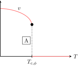
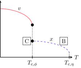
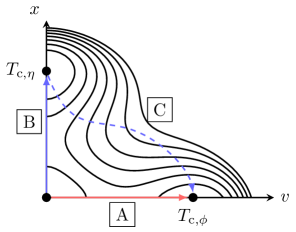
Figure 1: Multi-step transition for the Higgs ($\phi$) with background field $v$ and complex singlet ($\eta$) scalar with background field $x$ (cf. eq. (3.3)). The two left plots trace the $T$-dependence of the minima of $x$ and $v$. A single step (A) transitions from a symmetric to the Higgs phase at the critical temperature $T_{{\mbox{\scriptsize c}},\phi}$. During a two-step transition, one transitions first to the singlet direction (B) at the critical temperature $T_{{\mbox{\scriptsize c}},\eta}$ before transitioning to the Higgs direction at $T_{{\mbox{\scriptsize c}},\phi}$ (C). The contour lines in the right plot schematically depict the effective potential.

We focus on locating regions of first-order phase transitions, since we want to determine regions of the model parameter space where both dark matter and a strong phase transition are simultaneously possible.

Determining the character of phase transition in perturbation theory is not entirely reliable. A classic example is the SM itself. There a perturbative treatment – based on finding a discontinuity in the Higgs background field at the critical temperature – indicates a weakly first-order phase transition for Higgs masses $\gtrsim 70$ GeV. Non-perturbative studies [76, 77, 78, 79, 80] demonstrated that for such large Higgs masses, the SM has no thermal phase transition. Instead a crossover takes place, one where the system transitions smoothly from the symmetric to broken Higgs phase.

In the SM, the potential barrier that separates symmetric and Higgs phase is generated radiatively by loop corrections and non-existent at tree-level. The situation differs when analysing the complex singlet $\eta$ as two-step transitions allow for a barrier already at tree-level due to a non-vanishing background in singlet direction. It is these two-step transitions that we investigate in this work.

We find the global minimum of the potential as a function of the temperature, and determine the critical temperature from a condition that minima are discontinuous. Regions of strong first-order phase transitions can be identified by the condition $v_{3,c}/\sqrt{T_{{\rm c},\phi}}\geq 1$, where $v_{3}=v/\sqrt{T}$ relates the background fields of the 3d EFT and 4d parent theory; see eg. [22] for an application of this strategy. Since this condition is gauge-dependent, it lacks direct physical meaning – we determine it in Landau gauge. However, it can give an indicative estimate for the order parameters of the phase transition. A theoretically more robust analysis utilises the discontinuity of scalar condensates [82] at the critical temperature, that can be computed in a gauge-invariant manner [81, 38, 73]. Here, we choose a practical approach in terms of background fields [73], and expect that locating FOPT regions is insensitive to this choice.

Our result for a strong FOPT region is shown in fig. 2 in the case of a decoupled dark sector ($y=0$).

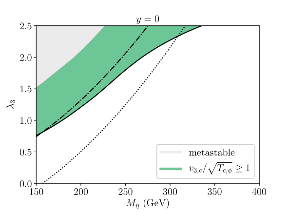
Figure 2: Region of strong two-step phase transitions in the limit of decoupled dark matter ($y=0$) and fixed $\lambda_{2}=1.25$. The analysis uses a perturbative estimate via discontinuous background fields at the critical temperature $T_{{\rm c},\phi}$. We show $v_{3,{\rm c}}/\sqrt{T_{{\rm c},\phi}}=1$ as a solid black line and $v_{3,{\rm c}}/\sqrt{T_{{\rm c},\phi}}>1$ as a green band that increases towards the grey region. There the electroweak minimum of the zero-temperature tree-level potential is not global. The strongest transitions reside in a region of negative singlet mass parameter between the grey region and $\mu_{\eta}=0$ line (dash-dotted). The dotted contour $\mu_{\eta}=0.5\,\pi T$ at fixed $T=100$ GeV is used to estimate the validity of the EFT construction, that assumes a light singlet. To the right of this line, such an assumption is compromised and $\mu_{\eta}\sim\pi T$.

In this plot, we vary the singlet mass and portal coupling for fixed $\lambda_{2}=1.25$. In the grey region (top left), the minimum in Higgs direction is not global at zero temperature, and the Higgs phase is metastable. The green band depicts a FOPT region and lies in a two-step transition regime, where above $T_{{\rm c},\phi}$ the singlet has a non-zero background field ($x_{3}$) at the global minimum. The dash-dotted line depicts a vanishing singlet mass parameter $\mu_{\eta}=0$, and the FOPT region lies in the vicinity of that line. The dotted line ($\mu_{\eta}=0.5\,\pi T$, $T=100$ GeV) qualitatively confines the region of validity of the EFT construction. To the right, the singlet mass parameter becomes hard $\mu_{\eta}\sim\pi T$, non-dynamical in the 3d EFT, and should be integrated out along with the non-zero Matsubara modes. From this observation, we cannot trust our result for the upper right FOPT region, and limit our study to $\lambda_{3}<2.5$ and $M_{\eta}<400$ GeV. For this qualitative guidance, we fixed $T=100$ GeV which is a conservative lower bound for $T_{{\rm c},\eta}$ that we find in the FOPT region. By varying $\lambda_{2}$, the FOPT region moves moderately in the $(M_{\eta},\lambda_{3})$-plane, but the general trend remains. For fixed $M_{\eta}$ and $\lambda_{3}$, reducing $\lambda_{2}$ weakens the transition.

While the parameters of the scalar potential ($\mu^{2}_{\eta}$, $\lambda_{3}$, $\lambda_{2}$) dominate the phase structure, the thermodynamic properties are also influenced by the presence of a dark sector when $y\neq 0$. This effect is illustrated in fig. 3 for $y=1$ and two choices of $M_{\chi}$.

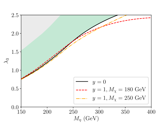
Figure 3: Contours $v_{3,{\rm c}}/\sqrt{T_{{\rm c},\phi}}=1$ for non-vanishing $y$ and two different hypotheses for $M_{\chi}=180$ GeV (dashed) and $M_{\chi}=250$ GeV (dash-dotted) at fixed $\lambda_{2}=1.25$. The region above the shown contour lines, $v_{3,{\rm c}}/\sqrt{T_{{\rm c},\phi}}>1$, corresponds to a strong phase transition. Only the band corresponding to $y=0$ is shaded.

The FOPT region stretches from the dashed (dash-dotted) line to the grey region, respectively (only the $y=0$ FOPT band is shaded). A non-zero $y$ mildly affects the region of a strong transition which is qualitatively the same as at $y=0$ (solid line). This is because the dark sector modifies the dimensional reduction matching relations merely at NLO (cf. eqs. (A.2) and (A.2)), and the transition is driven by the portal sector parameters. However, the different $y$ and $M_{\chi}$ contours behave non-trivially as a function of $M_{\eta}$ and $\lambda_{3}$ and e.g. cross the solid black ($y=0$) line. Here, we refrain from further exploring the dependence of the FOPT region on $(y,M_{\chi})$, but will inspect their role in sec. 5, when discussing the overlap with parameter regions that produce the observed dark matter abundance.

Studying the nucleation of the new stable vacuum of the theory is the next step in the analysis. Here, we do not compute the bubble nucleation rate but address some of the complications that can arise. The full FOPT regions in figs. 2 and 3 are not viable for a cosmological electroweak phase transition, as nucleation from the metastable singlet phase does not necessarily complete. Since we do not compute the bubble nucleation rate, we are unable to discriminate these unviable regions from those where nucleation completes. These unviable regions can be expected to lie near the metastability region at zero temperature. Our purely perturbative analysis is unable to find one-step transitions, since non-perturbative studies are required to discriminate first-order and crossover transitions. However, in analogy to [70, 83, 72, 84, 85], we could find these regions by integrating out the singlet in regions of parameter space where it is hard or soft near the critical temperature. For the resulting SM-like 3d EFT, the phase diagram is known non-perturbatively [77]. However, we do not perform such analyses here. Due to its relevance for dark matter production, we determined the typical critical temperature of the phase transition to be $110~{}{\rm GeV}\lesssim T_{{\mbox{\scriptsize c}},\phi}\lesssim 155~{}{\rm GeV}$ inside the green band in figs. 2 and 3.

Another subtlety in this model is that the nucleation temperature $T_{\rm n}$ could be significantly below the critical temperature $T_{\rm c}$. Such a potentially large degree of supercooling [86] could source bubble walls that are extremely relativistic and affect a successful EWBG [87]. Nucleation could also be affected by the formation of topological defects. One example are cosmic strings [88], which are generated due to the $\eta$-broken phase of the Abelian ${\rm U(1)}_{\mbox{\tiny\rm{Y}}}$ symmetry. Investigating the resulting nucleation dynamics for this model is left for future work on the subject.

4 Dark matter energy density

The dark matter model introduced in eq. (2.1) can account for the observed energy density through different production mechanisms in the early universe. The two main paradigms are freeze-out [89, 90] and freeze-in [91, 92]. The strategy to distinguish between the two options is to inspect the coupling of the actual DM particle, namely the Yukawa coupling $y$ in the portal interaction eq. (2.5). In this section, we use the physical particle masses and indicate them with $M_{i}$ for each species.

For $y$-values of the order of the electroweak SM gauge couplings, the dark fermion $\chi$ and anti-fermion $\bar{\chi}$ are in thermal equilibrium in the early universe plasma. DM particles follow an equilibrium abundance when the temperature is larger than their mass, that is also maintained when dark states enter a non-relativistic regime. Dark matter is mainly depleted by pair annihilations, which are very efficient up until $T/M_{\chi}\approx 1/25$. Around this temperature, dark particles decouple and their comoving abundance is frozen ever since [89, 90].

For values $y\lesssim\mathcal{O}(10^{-7})$ [95, 92, 96, 97, 98], dark matter particles never reached thermal equilibrium due to their tiny coupling with the surrounding thermal bath. This is in contrast with the central assumption of the freeze-out mechanism. The dark matter is feebly interacting and the production proceeds via freeze-in. In this case, dark matter particles are generated through various processes, that comprise decays of a heavier accompanying state in the dark sector, and $2\to 2$ scatterings that may involve SM particles. Dark matter particles only appear in the final state of the relevant reactions, and their abundance increases over the thermal history up until the production rate is efficient. Depending on the model parameters, in particular the mass splitting between the Majorana fermion and the heavier scalar, the super-WIMP mechanism contributes to a later-stage dark matter production through the decays of the frozen-out $\eta$ population [99, 100].

This work focuses on the freeze-out scenario, since we are also interested in shedding light on the effect of a sizeable Yukawa coupling $y$ on the EWPT. Yukawa coupling sizes of $y\lesssim\mathcal{O}(10^{-7})$ required for freeze-in will render Majorana fermions numerically irrelevant for computing the phase transition thermodynamics. A complementary production through freeze-in is postponed for future work. We describe the main differences with the freeze-out case and corresponding challenges in deriving the DM energy density in sec. 4.2.

4.1 Freeze-out

Three classes of processes are relevant for pair annihilations in the present model. One of them are pair annihilations of dark fermions. In addition, the presence of additional states that connect the dark sector with the SM can significantly alter the annihilation cross section [101, 90, 102, 45]. Here, the role of the co-annihilating partner is played by the $\eta$ scalar. Co-annihilations, i.e. processes with $\eta$ and $\chi$ as initial states, and scalar-pair annihilations are typically relevant for a relative mass splitting of $\Delta M/M_{\chi}\sim 0.2$, which is mildly model-dependent when assessed more precisely. In general, small mass splittings correspond to a population for $\eta$ as abundant as that of the dark fermion. Therefore, the dynamics of the $\eta$ particles is as important as that of $\chi$. Due to fast conversions as driven by the Yukawa coupling $y$, the two populations are in thermal contact [93, 103]. Conversely, for large mass splittings, the equilibrium abundance of the scalar is suppressed by $e^{-\Delta M/T}$ with respect to the lighter species, without impacting the annihilation pattern.

Pair annihilations of the dark fermion give a $p$-wave leading contribution; cf. eq. (B.1). This is a result of the chiral suppression of velocity-independent Majorana fermion pair annihilations typical for this model [45, 104]. Hence, co-annihilation processes as well as pair-annihilations of singlet scalars, which feature velocity-independent annihilation channels, dictate the evolution of the dark matter energy density abundance for small mass splittings [45, 103]. This is even more pronounced when considering for EWPT in sec. 3, a non-vanishing Higgs portal coupling ($\lambda_{3}\sim\mathcal{O}(1)$), that opens up additional channels for $\eta\eta^{\dagger}$ annihilations. We also include the Higgs-portal coupling contribution to the scalar mediator annihilations, that are often neglected for the model at hand (an exception is ref.[105]). We include them in the numerical extraction of the energy density, and list the expression of the corresponding cross sections in the appendix B.

We assume that $M_{\chi}\gtrsim 100$ GeV when computing cross sections, and exploring the parameter space. This is mainly motivated by the excluded regions reported in ref. [45] from the LEP-SUSY working group [106, 107, 108] and further improvements performed at the LHC [53, 54]. Since in this model $M_{\eta}>M_{\chi}$, the in-vacuum masses of the leptons are always negligible with respect to the dark matter particle and the scalar mediator. To affect the electroweak crossover, the mass of the additional scalar cannot be too large (cf. sec. 3) and in this section we consider $M_{\eta}\lesssim 1$ TeV. Once again, since $M_{\chi}<M_{\eta}$, and the freeze-out occurs for $M_{\chi}/T\sim 25$, the typical temperatures are below the electroweak transition $T_{{\mbox{\scriptsize c}},\phi}$ as estimated in sec. 3. Therefore, we work in the broken electroweak theory where the Higgs mechanism is active and responsible for the mass generation of the SM fermions and gauge bosons.

Whenever the conversion processes between the actual DM and the heavier co-annihilating partner are efficient during freeze-out, which is the case for typical $y$ values adopted here, the effect of accompanying states can be captured by a single Boltzmann equation [89, 90]

$$\frac{dn}{dt}+3Hn=-\langle\sigma_{{{\mbox{\scriptsize eff}}}}\,v_{\mbox{\scriptsize rel}}\rangle(n^{2}-n^{2}_{{{\mbox{\scriptsize eq}}}})\;,$$ (4.1)

where the left side is the covariant time derivative in an expanding background, $H$ is the Hubble rate of the expanding universe, $v_{\mbox{\scriptsize rel}}$ is the relative velocity of the annihilating pair, and $n$ denotes the overall number density of both states $\chi$ and $\eta$. Then, the total equilibrium number density, which accounts for both the particle species $\chi$ and $\eta$, is

$$n_{{\rm{eq}}}=\int_{{\bf p}}e^{-E_{p,\chi}/T}\Bigl{[}g_{\chi}+g_{\eta}e^{-\Delta M_{{\mbox{\tiny\rm{$T$}}}}/T}\Bigr{]}\;,\quad E_{p,\chi}=M_{\chi}+\frac{{\bf p}^{2}}{2M_{\chi}}\;,$$ (4.2)

where the internal degrees of freedom are $g_{\chi}=2$ for the fermion (2 spin polarisations, Majorana fermion) and $g_{\eta}=2$ for the scalar (particle and antiparticle, complex scalar singlet). The mass difference $\Delta M_{{\mbox{\tiny\rm{$T$}}}}$ gets the vacuum contribution, $\Delta M=M_{\eta}-M_{\chi}$, and a thermal correction in the non-relativistic limit (see also refs. [109, 110, 100])

$$\Delta M_{{\mbox{\tiny\rm{$T$}}}}=\Delta M +\frac{\lambda_{3}}{M_{\eta}}\int_{{\bf p}}\frac{n_{\mbox{\tiny\rm{B}}}(E_{p,\phi})}{E_{p,\phi}}+\frac{g_{1}^{2}Y_{\eta}^{2}}{4M_{\eta}}\int_{{\bf p}}\left(\frac{\tilde{c}^{2}\,n_{\mbox{\tiny\rm{B}}}(E_{p,\gamma})}{E_{p,\gamma}}+\frac{\tilde{s}^{2}\,n_{\mbox{\tiny\rm{B}}}(E_{p,{\mbox{\tiny\rm{$Z$}}}})}{E_{p,{\mbox{\tiny\rm{$Z$}}}}}\right)$$

$$-\frac{g_{1}^{2}Y_{\eta}^{2}}{32\pi}\left(\tilde{c}^{2}M_{{\mbox{\tiny\rm{$T$}}},\gamma}+\tilde{s}^{2}M_{{\mbox{\tiny\rm{$T$}}},{\mbox{\tiny\rm{$Z$}}}}-s^{2}M_{\mbox{\tiny\rm{$Z$}}}\right)\;,$$ (4.3)

where $E_{p,i}=\sqrt{{\bf p}^{2}+M_{{\mbox{\tiny\rm{$T$}}},i}^{2}}$. The thermal contributions come from the gauge bosons and Higgs tadpoles, whereas the latter arises from the contribution of screened soft gauge bosons at the scale $gT$ (also known as Salpeter correction [111]). The relevant thermal masses $M_{{\mbox{\tiny\rm{$T$}}},i}$ and weak mixing angles are listed in eqs. (B.14), (B.16), (B.13) and (B.18). The integral measure is defined as $\int_{{\bf p}}\equiv\int{\rm d}^{3}{\bf p}/(2\pi)^{3}$, and the effective thermally averaged annihilation cross section reads [90]

$$\langle\sigma_{{\rm{eff}}}v_{\mbox{\scriptsize rel}}\rangle=\sum_{i,j}\frac{n^{{\mbox{\scriptsize eq}}}_{i}\,n^{{\mbox{\scriptsize eq}}}_{j}}{(\sum_{k}n_{k}^{{\mbox{\scriptsize eq}}})^{2}}\langle\sigma_{ij}v_{\mbox{\scriptsize rel}}\rangle\;.$$ (4.4)

Here $\langle\sigma_{{\rm{eff}}}v_{\mbox{\scriptsize rel}}\rangle$ includes all combinations for the annihilating pairs, namely $\chi\chi$, $\chi\eta$, $\eta\eta^{\dagger}$, $\eta\eta$ and their conjugates when relevant. Conventionally, it is calculated by thermally averaging the in-vacuum cross sections over the centre-of-mass energies in the thermal environment [89, 90]. The in-vacuum annihilation cross sections in the broken phase of the electroweak symmetry can be found in the appendix B. The diagrams for the Majorana fermion (co-)annihilations, and a representative process for pair-annihilation are collected in fig. 4.

$$\mathcal{M}_{\chi\chi\to e\bar{e}} =\;\parbox[c]{31.5pt}{\begin{picture}(31.5,21.0)(0.0,0.0)\ignorespaces\ignorespaces{\put(0.0,0.0){}}\ignorespaces {\put(0.0,0.0){}}\ignorespaces {\put(0.0,0.0){}}\ignorespaces{\put(0.0,0.0){}}\ignorespaces {\put(0.0,0.0){}}\ignorespaces\end{picture}}\;+\;\parbox[c]{42.0pt}{\begin{picture}(42.0,21.0)(0.0,0.0)\ignorespaces\ignorespaces{\put(0.0,0.0){}}\ignorespaces{\put(0.0,0.0){}}\ignorespaces {\put(0.0,0.0){}}\ignorespaces {\put(0.0,0.0){}}\ignorespaces{\put(0.0,0.0){}}\ignorespaces {\put(0.0,0.0){}}\ignorespaces\end{picture}}\;\;,$$

$$\mathcal{M}_{\chi\eta^{\dagger}\to eZ(\gamma)} =\;\parbox[c]{31.5pt}{\begin{picture}(31.5,21.0)(0.0,0.0)\ignorespaces\ignorespaces {\put(0.0,0.0){}}\ignorespaces {\put(0.0,0.0){}}\ignorespaces {\put(0.0,0.0){}}\ignorespaces{\put(0.0,0.0){}}\ignorespaces {\put(0.0,0.0){}}\ignorespaces\end{picture}}\;+\;\parbox[c]{42.0pt}{\begin{picture}(42.0,21.0)(0.0,0.0)\ignorespaces\ignorespaces {\put(0.0,0.0){}}\ignorespaces {\put(0.0,0.0){}}\ignorespaces {\put(0.0,0.0){}}\ignorespaces{\put(0.0,0.0){}}\ignorespaces{\put(0.0,0.0){}}\ignorespaces\end{picture}}\;\;,$$

$$\mathcal{M}_{\eta\eta^{\dagger}\to\gamma\gamma} =\;\parbox[c]{31.5pt}{\begin{picture}(31.5,21.0)(0.0,0.0)\ignorespaces\ignorespaces {\put(0.0,0.0){}}\ignorespaces {\put(0.0,0.0){}}\ignorespaces {\put(0.0,0.0){}}\ignorespaces {\put(0.0,0.0){}}\ignorespaces\end{picture}}\;+\;\parbox[c]{31.5pt}{\begin{picture}(31.5,21.0)(0.0,0.0)\ignorespaces\ignorespaces {\put(0.0,0.0){}}\ignorespaces {\put(0.0,0.0){}}\ignorespaces {\put(0.0,0.0){}}\ignorespaces {\put(0.0,0.0){}}\ignorespaces {\put(0.0,0.0){}}\ignorespaces\end{picture}}\;+\;\parbox[c]{42.0pt}{\begin{picture}(42.0,21.0)(0.0,0.0)\ignorespaces\ignorespaces {\put(0.0,0.0){}}\ignorespaces {\put(0.0,0.0){}}\ignorespaces {\put(0.0,0.0){}}\ignorespaces {\put(0.0,0.0){}}\ignorespaces {\put(0.0,0.0){}}\ignorespaces {\put(0.0,0.0){}}\ignorespaces\end{picture}}\;\;.$$

Figure 4: Diagrams for the dark matter pair annihilation and co-annihilation with the singlet scalar. The dark fermion $\chi$ is displayed by a double-solid line, the complex scalar $\eta$ by an arrowed double-dashed line, the SM lepton $e$ by an arrowed solid line, and photons and $Z$-bosons by wiggly lines.

The impact of the processes $\chi\eta$ and $\eta\eta^{\dagger}$ is controlled by the functional dependence of the equilibrium number densities in eq. (4.4), that gives $\langle\sigma_{{{\mbox{\scriptsize eff}}}}v_{\mbox{\scriptsize rel}}\rangle\approx\langle\sigma_{\chi\chi}v_{\mbox{\scriptsize rel}}\rangle+\langle\sigma_{\chi\eta}v_{\mbox{\scriptsize rel}}\rangle e^{-\Delta M_{\mbox{\tiny\rm{$T$}}}/T}+\langle\sigma_{\eta\eta^{\dagger}}v_{\mbox{\scriptsize rel}}\rangle e^{-2\Delta M_{\mbox{\tiny\rm{$T$}}}/T}$. This manifests that a large ration of mass splittings over temperature (at freeze-out and later stages) suppresses the importance of the co-annihilations.

The Boltzmann equation (4.1) is then as usual recast in terms of the yield parameter $Y=n/s$, where $s=2\pi^{2}h_{{\mbox{\scriptsize eff}}}\,T^{3}/45$ is the entropy density, and the time evolution is traded for the variable $z=M_{\chi}/T$. As for the temperature-dependent relativistic degrees of freedom $h_{{\mbox{\scriptsize eff}}}$ entering the entropy density, we use the SM values from ref. [112]. The relativistic degrees of freedom for the energy density $g_{{\mbox{\scriptsize eff}}}$, that enter the Hubble rate $H=\sqrt{8\pi e/3}\,M_{\mbox{\tiny\rm{Pl}}}$, where $e=\pi^{2}T^{4}g_{{\mbox{\scriptsize eff}}}/30$, are also taken from [112].

4.1.1 $\eta\eta^{\dagger}$ annihilations

An additional discussion is in order for the $\eta\eta^{\dagger}$ annihilations. The scalar particle $\eta$ interacts with the ${\rm U(1)}_{\mbox{\tiny\rm{Y}}}$ gauge boson $B_{\mu}$ and the Higgs boson. The former interaction can also be understood in terms of the mass-diagonal fields i.e. the $Z$-boson and photon. Since the pair-annihilations happen in a non-relativistic regime, the scalar (anti-)particles are heavy and slowly moving in the thermal plasma. In this setting, repeated soft exchanges of the force carriers (vector or scalar particles) can significantly alter the annihilation cross section of the incoming $\eta$ pair. Two effects play an important role: the Sommerfeld enhancement [41, 113, 114] and bound-state formation [115, 42]. Their main phenomenological consequence is that the annihilations are boosted for small velocities. Moreover, whenever bound states are formed and not effectively dissociated or melted away in the thermal plasma, they provide an additional process for the depletion of DM particles in the early universe.

The annihilation rate for the accompanying scalar contributes to the overall cross section in eq. (4.4) in the co-annihilation regime. In turn, the overall cross section enters the extraction of the dark matter energy density.

boson		$\mathcal{V}(r)$		coupling
photon		$\mathcal{V}_{\gamma}(r)=-\frac{\alpha_{\gamma}}{r}\,e^{-rM_{{\mbox{\tiny\rm{$T$}}},\gamma}}$		$\alpha_{\gamma}=\alpha_{{\mbox{\scriptsize em}}}\frac{Y_{\eta}^{2}}{4}\left(\frac{\tilde{c}_{w}}{c_{w}}\right)^{2}$
$Z$-boson		$\mathcal{V}_{{\mbox{\tiny\rm{$Z$}}}}(r)=-\frac{\alpha_{Z}}{r}e^{-rM_{{\mbox{\tiny\rm{$T$}}},{\mbox{\tiny\rm{$Z$}}}}}$		$\alpha_{{\mbox{\tiny\rm{$Z$}}}}=\alpha_{{\mbox{\scriptsize em}}}\frac{Y_{\eta}^{2}}{4}\left(\frac{\tilde{c}_{w}}{c_{w}}\right)^{2}\tan^{2}(\tilde{\theta}_{w})$
$H$-boson		$\mathcal{V}_{\phi}(r)=-\frac{\alpha_{\phi}}{r}e^{-rM_{{\mbox{\tiny\rm{$T$}}},\phi}}$		$\alpha_{\phi}=\frac{\lambda_{3}^{2}v_{\mbox{\tiny\rm{$T$}}}^{2}}{16\pi M_{\eta}}$

Table 1: Attractive potentials and fine structure constants for the ${\rm U(1)}_{\mbox{\tiny\rm{Y}}}$-charged scalar $\eta$ from the different force mediators. We abbreviate the Weinberg angle at $T=0$ with $c\equiv\cos(\theta_{w})$ in eq. (B.13) and at finite-temperature with $\tilde{c}\equiv\cos(\tilde{\theta}_{w})$ in eq. (B.18); $v_{\mbox{\tiny\rm{$T$}}}$ is the temperature-dependent Higgs VEV in eq. (B.14). Here, $e=g_{1}\cos(\theta_{w})$, with $\alpha_{{\mbox{\scriptsize em}}}=e^{2}/(4\pi)$.

For our case, the scalar annihilations can be affected by the photon, $Z$-boson an Higgs boson induced potentials, collected in tab. 1. In the broken phase of the electroweak symmetry, and in a thermal environment of the early universe, some quantities become temperature-dependent. By following phenomenological prescriptions [116, 117], one finds that

• the Higgs VEV $v$ and the Higgs mass depend on the temperature;

• the temporal part of the gauge bosons acquire thermal masses, also the photon;

• the weak mixing angle $\theta_{w}$, or Weinberg angle, evolves with the temperature.

We include these effects in the static potentials when estimating the Sommerfeld factors. In appendix B.2 we collect the relevant definitions, whereas we refer to [116] for a more detailed discussion.

We follow the approach of ref. [114] to numerically extract the Sommerfeld enhancement due to the exchange of a Higgs boson, photon, and $Z$-boson – both for the $s$- and $p$-wave annihilations. We also include temperature-dependent masses for the force carriers that are indicated as $M_{{\mbox{\tiny\rm{$T$}}},\phi}$ in eq. (B.14) and $M_{{\mbox{\tiny\rm{$T$}}},\gamma}$, $M_{{\mbox{\tiny\rm{$T$}}},{\mbox{\tiny\rm{$Z$}}}}$ in eq. (B.16), and reproduce the values $M_{\phi}=125.1$ GeV, $M_{\gamma}=0$, and $M_{\mbox{\tiny\rm{$Z$}}}=91.2$ GeV for $T\to 0$. In our treatment, also the photon induces a Yukawa-like potential, rather than a Coulomb potential, for sufficiently high temperatures corresponding to non-negligible thermal masses. The temperature-dependent masses are shown in fig. 5 (left).

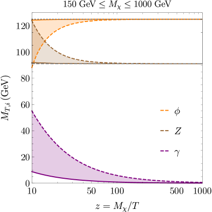
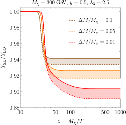
Figure 5: Left: Thermal masses for the gauge and Higgs bosons and their in-vacuum counterparts (grey lines). Right: Ratio of the DM yields with and without the Sommerfeld enhancement for the co-annihilating scalar particle. The bands show the impact of a Yukawa-like potential when a thermal mass of the photons is included (solid lines).

Here we consider the dark matter mass to vary between $150~{}{\rm GeV}\leq M_{\chi}\leq 10^{3}~{}{\rm GeV}$, and the solid (dashed) lines stand for the smallest (largest) masses and temperatures. The grey dotted lines indicate the in-vacuum masses for the Higgs boson and $Z$-boson. Thermal masses differ by 5% of the corresponding in-vacuum values at the chemical freeze-out temperature $T\simeq M_{\chi}/25$. For the photon, a thermal mass can potentially be more relevant, since at $T=0$ the photon is massless. However, we find the Sommerfeld factor corresponding to a Yukawa-like potential, with a finite photon mass, to be smaller by a few-per-cent than the Sommerfeld factor computed in the Coulomb limit. We crosscheck the numerical extraction of the Sommerfeld factors with the formalism of [117], that relies on determining the spectral function of the $\eta$-$\eta^{\dagger}$ pair, and obtain compatible results.

The ratio between the dark matter yield $Y_{{\mbox{\tiny\rm{SE}}}}$($Y_{{\mbox{\tiny\rm{LO}}}}$) with(out) the Sommerfeld enhancement from the $\gamma$, $Z$ and Higgs boson exchange is shown in fig. 5 (right). The dominant Sommerfeld enhancement is induced by the photon exchange in the mass range relevant for our work, namely $M_{\chi},M_{\eta}\lesssim 1$ TeV. To show the effect of a finite (thermal) photon mass, we show the DM yields as obtained with the Sommerfeld factors in the Coulomb limit (dashed lines) and for the Yukawa-like potential (solid lines). The difference between the two cases is small, with an effect of $\sim 1\%$ on the yield ratio. As expected, the screened potential corresponds to less effective annihilations and solid lines exceed the dashed ones. Our assessment shows that the $T=0$ treatment is well suited for the relic density extraction in this model in the freeze-out scenario. One can safely use the $T\to 0$ limit of the potentials (see e.g. ref. [105] for the same model). We fixed the dark matter mass to $M_{\chi}=300$ GeV, considered three relative mass splittings $\Delta M/M_{\chi}\in\{0.1,0.05,0.01\}$, and fixed the Higgs-portal coupling to $\lambda_{3}=2.5$. A non-vanishing scalar portal coupling induces many processes that add up to the scalar-pair annihilations; see cross sections in appendix B. In agreement with the co-annihilation scenario [101, 102, 45], the smaller the splitting the larger the effect of the $\eta$-$\eta^{\dagger}$ annihilations. For this choice of the dark matter mass and the Yukawa coupling $y$, the Sommerfeld enhancement reduces the dark matter abundance by 6–11% depending on the mass splitting. We find that varying the DM mass $M_{\chi}\in[10^{2},10^{3}]$ GeV and $y\in[0.1,2]$ changes $Y_{{\mbox{\tiny\rm{SE}}}}/Y_{{\mbox{\tiny\rm{LO}}}}$ only slightly, whereas decreasing $\lambda_{3}$ impacts the yield ratio stronger (with a less important Sommerfeld enhancement).

The situation is more intricate for the bound-state effects. First, the potentials are Yukawa-like and it is not obvious if they are sufficiently long-ranged with respect to the energy scales at play. A reasonable estimate can be obtained by demanding that the screening length is not smaller than the typical bound-state size, i.e. $1/M_{X}\gtrsim a_{0}$, where the Bohr radius is $a_{0}=2/(M_{\eta}\alpha_{X})$ with $X=\gamma,Z,\phi$, and the corresponding fine structure constant is $\alpha_{X}$. More precisely, one can exploit the numerical evaluation that demands for a ground state to form, that reads $1/M_{X}\geq 0.84a_{0}$ [118]. Then, for the $Z$-boson induced bound states, we obtain a lower bound $M_{\eta}\gtrsim 70$ TeV, which is higher than the masses we are interested in (our estimate compares well with the one detailed recently in ref. [105]). For the Higgs boson, we find that even for the largest coupling that we allowed, $\lambda_{3}=3.0$, the bound gives $M_{\eta}\gtrsim 5$ TeV. Therefore, only the photon exchange can sustain the formation and existence of bound states in the relevant mass and temperature range.

The annihilation of a $\eta$-$\eta^{\dagger}$ pairs as bound states can efficiently occur only if they are not dissociated by the interactions with the medium constituents. Owing to some similarities with heavy quarkonium in medium, where the bound-state dynamics is driven by gluo-dissociation [119] and the dissociation by inelastic parton scattering [120], the model at hand features similar processes involving photons. See refs. [121, 109, 122, 123] for applications to dark matter. The first dissociation process entails a thermal photon hitting the $\eta$-$\eta^{\dagger}$ pair in a bound-state and, if sufficient energy is available, breaking it into an unbound above-threshold pair. The second dissociation process comes as a $2\to 2$ scattering reaction, where the particles in the thermal bath transfer energy/momenta to the heavy $\eta$-$\eta^{\dagger}$ pair through a photon exchange, turning a bound-state into an unbound one. Since we have checked that a thermal mass for the photon gives a practically negligible effect on the DM abundance when including it the Sommerfeld enhancement (see right panel in fig. 5), we remain in the Coulombic regime and treat the photon as massless. This approximation enables us to adapt former derivations for the bound-state formation cross section [121], from which the dissociation rate $\Gamma_{{\mbox{\scriptsize bsd}}}$ can be obtained via the Milne relation [124]; see appendix B for details on the rates and Boltzmann equation for bound states. We find that the bound-state effects are fairly small for $M_{\eta}\lesssim 1$ TeV and an electroweak coupling strength $\alpha_{\gamma}\sim\mathcal{O}(10^{-2})$. In fact, we obtain a correction of 1–2% with respect to the yield where the Sommerfeld enhancement is already accounted for. This is consistent with the analysis in ref. [42], and confirmed by the studies [121, 109, 122].

4.1.2 Numerical results and parameter space

The results for the model parameter space compatible with the observed dark matter energy density $\Omega_{{\mbox{\tiny\rm{DM}}}}h^{2}\big{|}_{{\mbox{\scriptsize obs.}}}=0.1200\pm 0.0012$ [125] are shown in this section. The predicted DM energy density depends on the model parameters, namely $\left\{M_{\chi},M_{\eta},y,\lambda_{3},\lambda_{2}\right\}$. At the order we are working, the $\eta$ self-coupling $\lambda_{2}$ enters the extraction of the DM energy density only through the renormalisation group equations (RGE), that provide the values of all couplings at a given energy scale; see eqs. (A.1)–(A.11). We consider different and complementary ways to visualise the parameter space compatible with $\Omega_{{\mbox{\tiny\rm{DM}}}}h^{2}\big{|}_{{\mbox{\scriptsize obs.}}}$.

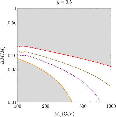
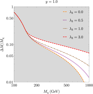
Figure 6: Parameter space in the $(M_{\chi},\Delta M/M_{\chi})$-plane compatible with the observed DM energy density as white area comprised between the orange dashed ($\lambda_{3}=0.0$) and red dashed ($\lambda_{3}=3.0$) curves.

A first visualisation of the parameter space as in fig. 6 was already adopted for the family of simplified models to which our model Lagrangian belongs, see e.g. [45, 126, 103]. To obtain the curves shown in fig. 6, we fix $y$ and $\lambda_{2}$, we trade $M_{\eta}$ with the relative mass splitting, and take $(M_{\chi},\Delta M/M_{\chi})$ as free parameters. We consider different values for the portal coupling $\lambda_{3}$. The effect of non-vanishing $\lambda_{3}$ allows for larger mass splittings since the overall cross section (4.4) is larger due to many additional annihilation processes enabled by the coupling $\lambda_{3}$. Moreover, co-annihilations are more relevant for smaller Yukawa couplings $y$ (compare panels in fig. 6). This effect arises for smaller dark matter masses and traces back to the relative importance of the various contributions to the cross section. The smaller $y$ the larger the relative importance of the pair annihilation of scalar pairs, that features $y$-independent annihilation channels.

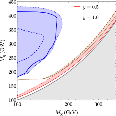
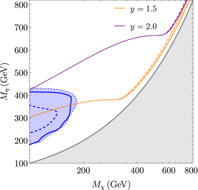
Figure 7: Coloured bands reproduce the observed energy density in the parameter space $(M_{\chi},M_{\eta})$; at $y=0.5$ and $y=1.0$ (left), as well as $y=1.5$ and $y=2.0$ (right). The solid (dashed) line corresponds to $\lambda_{3}=0.0$ ($\lambda_{3}=3.0$). The shaded grey area corresponds to $M_{\chi}<M_{\eta}$, which is not a viable option for the model. The collider-excluded regions for the different lepton flavours are the shaded blue areas from the ATLAS searches [53, 54] for the electron (solid), muon (dotted), and tau (dashed). For Majorana fermion masses $M_{\chi}>140\;(180)$ GeV when coupling to taus (muons), experimental limits are absent for $M_{\eta}$.

As a second option, we visualise the curves reproducing the observed DM energy density in the $(M_{\chi},M_{\eta})$-plane in fig. 7. To ensure the stability of the dark fermion, the grey area $M_{\chi}>M_{\eta}$ is not allowed in the model. The left panel includes two choices for the Yukawa coupling $y=0.5$ and $y=1.0$ with corresponding bands $\lambda_{3}\in[0.0,3.0]$ ($\lambda_{3}=0$ for solid lines, $\lambda_{3}=3.0$ for dashed lines). The larger effect of co-annihilations and $\eta$-pair annihilations for a smaller Yukawa coupling $y$ is also visible and results in a wider $y=0.5$ band (red) than the $y=1.0$ one (brown). The right panel shows corresponding bands that reproduce $\Omega_{{\mbox{\tiny\rm{DM}}}}h^{2}\big{|}_{{\mbox{\scriptsize obs.}}}$ at larger $y=1.5,2.0$. The sharp transition to the co-annihilation strip is visible as the transition from a line to a band, and is delayed to larger $M_{\chi}$ for larger $y$. We included the ATLAS exclusion limit at 95% confidence level for right-handed slepton searches at the LHC, in particular for the stau (dashed) [53] and for the smuon (dotted) and selectron (solid) [54] as excluded shaded blue regions in the parameter space. These constraints also apply to the simplified model since the experimental limits are obtained from the Drell-Yan production of the scalars, that decay promptly into a dark fermion and a lepton.

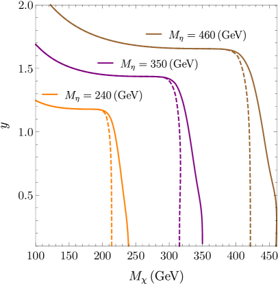
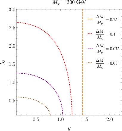
Figure 8: Left: Curves reproduce the observed energy density in the parameter space $(M_{\chi},y)$. Three benchmark values for the scalar mass $M_{\eta}\in\{240,350,460\}$ GeV are considered at $\lambda_{3}=3.0$ (dashed) and $\lambda_{3}=0$ (solid). Right: Curves in the parameter space $(y,\lambda_{3})$ for the DM mass $M_{\chi}=300$ GeV and different relative mass splittings $\Delta M/M_{\chi}$.

Two additional visualisations of the parameter space compatible with the observed energy density are offered in fig. 8. The left panel focuses on the $(M_{\chi},y)$-plane for three different values of the scalar mass $M_{\eta}\in\{240,350,460\}$ GeV for $\lambda_{3}=3.0$ (dashed) and $\lambda_{3}=0$ (solid). The behaviour of the curves can be understood by recalling the general form of the cross section for the scalar annihilations. On the one hand, for large values of the scalar-portal coupling, many contributions to the cross section $\langle\sigma_{\eta\eta^{\dagger}}v_{\mbox{\scriptsize rel}}\rangle$ are active and one can allow for large mass splittings. On the other hand, for $\lambda_{3}=0$ one has to require smaller mass splitting to compensate for a smaller cross section $\langle\sigma_{\eta\eta^{\dagger}}v_{\mbox{\scriptsize rel}}\rangle$ such that the two masses $M_{\chi}$ and $M_{\eta}$ are almost degenerate. The right panel of fig. 8 shows the contours for $\Omega_{{\mbox{\tiny\rm{DM}}}}h^{2}\big{|}_{{\mbox{\scriptsize obs.}}}$ in the $(y,\lambda_{3})$-plane at fixed dark matter mass $M_{\chi}=300$ GeV. For the relative mass splitting $\Delta M/M_{\chi}=0.25$, beyond the co-annihilation strip, there is no dependence on $\lambda_{3}$ because of a suppressed scalar population at the time of freeze-out and later stages. Conversely, by progressively decreasing the splitting, the Yukawa and scalar-portal couplings become intertwined and the observed energy density can be realised by tuning one of the two couplings larger while decreasing the other.

4.2 Freeze-in

There is a two-fold motivation to not pursue a detailed analysis for the freeze-in parallel to the freeze-out mechanism. First, we want to assess the effect of a fermionic state coupled to the scalar sector, which undergoes a phase transition. Typical values of the Yukawa coupling $y$ required for freeze-in production would completely decouple the fermion $\chi$ from the thermodynamics of the phase transition. This is at variance with $y\sim\mathcal{O}(1)$ for the freeze-out scenario. Second, and most importantly, a reliable extraction of the parameter space of the model compatible with the observed DM energy density is highly non-trivial. In the following, we highlight further aspects in contrast with the freeze-out case.

The freeze-in production occurs in a complementary temperature regime than freeze-out, namely $T\gtrsim M_{\eta},M_{\chi}$. The latter is understood as the in-vacuum physical masses. In this model, and rather in general for freeze-in produced DM, dark particles are generated through the decays of a heavier accompanying state, here $\eta\to\chi e$, and $2\to 2$ scatterings that may involve SM particles. If one assumes a vanishing initial abundance for the DM, the tiny couplings with other fields prevent DM to ever reach chemical equilibrium. Hence, dark matter particles only appear in the final state of the relevant processes, and their abundance builds up and increases over the thermal history. The production takes place over a wide temperature range, that includes $T\gg M_{\eta},M_{\chi}$. Hence, thermal effects can be relevant.

The impact of thermal masses on freeze-in produced dark matter has been studied recently by focusing on decay processes that would be forbidden at zero temperature. Instead, such processes are realised in a thermal environment [130, 131, 132, 133, 100]. Moreover, for the quark-philic model where the DM is coupled to a quark via a QCD-charged scalar, the contribution to the dark matter production rate from multiple soft scatterings at high temperature, oftentimes called the Landau-Pomeranchuk-Migdal (LPM) effect [134, 135, 136], can drastically change the DM production rate depending on the relative mass splitting $\Delta M/M_{\chi}$ [100]. Such resummations capture the quantum mechanical interference of collective plasma phenomena in a collinear kinematic regime at high temperature. The main result is that effective $2\to 1$ processes occur and enhance the production of the DM particle for $T\gg M_{\chi}$. In the present model one has $\eta\to\chi e$, $e\to\eta\chi$, and $\eta e\to\chi$.

At temperatures higher than the electroweak (crossover) transition, the dynamics of the scalar $\eta$ can be intricate. The scalar may also undergo a phase transition, and broken and symmetric phases can alternate along the thermal history (see two-step versus one-step transition in fig. 1). This induces a strong temperature dependence of the physical mass of $\eta$ and its interactions with other particles in the plasma. Hence, an accurate treatment of the scalar thermodynamics needs to be interfaced with the DM production along the thermal history to compute decays and scattering processes on a solid basis. See e.g. [140] for an implementation of these aspects for a scalar singlet DM coupled to the SM Higgs boson within a more phenomenological treatment of the EWPT.

For tiny $y$ couplings, two sources contribute to the overall DM energy density in this model [99, 94]. In addition to the freeze-in mechanism, that dominates at temperatures $T\gtrsim M_{\eta}$, instead the super-WIMP mechanism [141, 142] occurs much later in the thermal history at $T\ll M_{\eta}$. During the latter mechanism, the final abundance of $\eta$ particles is fixed by freeze-out dynamics, and dark matter is produced in the subsequent $\eta$ decay process $\eta\to\chi e$. Such a decay process will become efficient much later than the chemical freeze-out due to the minuscule coupling $y\ll 1$. The observed dark matter energy density is then given by

$$(\Omega_{{\mbox{\tiny\rm{DM}}}}h^{2})_{{\mbox{\scriptsize obs.}}}=(\Omega_{{\mbox{\tiny\rm{DM}}}}h^{2})_{{\mbox{\scriptsize freeze-in}}}+(\Omega_{{\mbox{\tiny\rm{DM}}}}h^{2})_{{\mbox{\scriptsize super-WIMP}}}\;.$$ (4.5)

We postpone extracting the DM energy density including LPM resummation, the effect of thermal masses, together with the interplay of the thermodynamics of the $\eta$ scalar to future studies. For recent investigations of freeze-in production, super-WIMP, and conversion-driven freeze-out of the model considered in our work, see ref. [94, 105]. There the above-mentioned effects have not been included.

5 Overlapping parameter space for phase transition and dark matter

This section investigates the joint model parameter space responsible for both the observed DM energy density and the EWPT. Thus, we explore to what extent the model allows, at the same time, for the observed energy density and a strong first-order phase transition. The main results are visualised in two ways.

The first option focuses on the $(M_{\eta},\lambda_{3})$-plane. There the ranges that mark a strong first-order phase transition are easier to understand (cf. sec. 3).

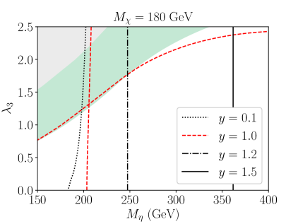
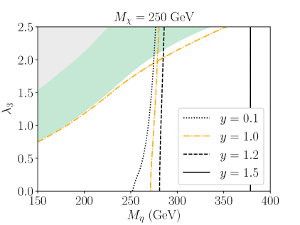
Figure 9: Overlay of contours for the observed DM abundance $\Omega_{{\mbox{\tiny\rm{DM}}}}h^{2}|_{{\mbox{\scriptsize obs.}}}$ (vertical lines) in the $(M_{\eta},\lambda_{3})$-plane, for $M_{\chi}=180$ GeV (left) and $M_{\chi}=250$ GeV (right). The green band features a strong phase transition for $y=0$ (cf. fig. 3). For $y=1$, we contour $v_{3,{\rm c}}/\sqrt{T_{{\rm c},\phi}}=1$ for $M_{\chi}=180$ GeV (red, dashed) and $M_{\chi}=250$ GeV (orange, dash-dotted). For $y=1$, above the intersection point of the red dashed and orange dash-dotted lines, a strong phase transition is compatible with the observed DM abundance.

Figure 9 provides the findings for two different hypotheses of the dark matter fermion mass $M_{\chi}=180$ GeV (left) and $M_{\chi}=250$ GeV (right). Such values evade the present-day collider searches for each lepton flavour (cf. fig. 7). For the EWPT, we show the metastable region (grey) and reference the FOPT region at $y=0$ as green as in fig. 3. Then, we contour $v_{3,{\rm c}}/\sqrt{T_{{\rm c},\phi}}=1$ corresponding to a non-vanishing dark-matter interaction with the scalar sector for $y=1.0$, $M_{\chi}=180$ GeV (red, dashed) and $y=1.0$, $M_{\chi}=250$ GeV (orange, dash-dotted). Since the trend extends also to larger $y$-values (cf. sec. 3), we merely provide the benchmark line for $y=1.0$.

For dark matter, the dotted, dash-dotted, dashed, and solid contours in the $(M_{\eta},\lambda_{3})$-plane reproduce $\Omega_{{\mbox{\tiny\rm{DM}}}}h^{2}|_{{\mbox{\scriptsize obs.}}}=0.1200$. The dependence between the two variables is rather mild and is progressively lost when increasing the Yukawa coupling $y$, which results in a straight vertical line (solid, $y=1.5$) in both panels. Small values of $y$ render $\chi\chi$ annihilations poorly effective (cf. sec. 4). Hence, the scalar pair annihilations, which are $\lambda_{3}$-dependent, drive the energy density and demand small mass splittings. This results in values of $M_{\eta}$ that tend to be close to $M_{\chi}=180$ GeV and $M_{\chi}=250$ GeV for small $y$ and $\lambda_{3}$. As long as $y$ increases, the $\chi\chi$ annihilations become more important, and one can allow for larger $M_{\eta}$ masses. For large enough $y$, the dependence on the scalar annihilations, and then on $\lambda_{3}$ is lost, as one may see from the straight vertical lines for $y=1.5$.

The bottom line of this comparison is the following. Some parameter regions of the model can account for the observed DM energy density and a strong first-order phase transition. The overlapping region widens for smaller dark fermion masses which also lies in the parameter space where the perturbative assessment for the phase transition is more reliable. Moreover, taking $y<0.1$ does not change the black dotted curve since the DM energy density is dominantly fixed by the scalar pair-annihilations already at $y=0.1$. Thus, the scalar mass $M_{\eta}$ is bound from below by the black dotted line whereas increasing $y>1.5$ would push $M_{\eta}\gtrsim 400$ loosing entirely the connection with the EWPT. The plot in fig. 10, shows the overlapping region (orange) for varying $y$ and is further discussed in the conclusions below.

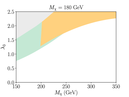
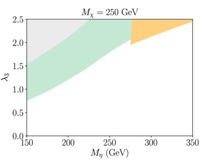
Figure 10: Overlapping regions (orange) of strong FOPT and observed dark matter energy density for fixed $M_{\chi}$ and $0.1<y<1.5$. The $y=0$ FOPT green band is adopted from fig. 2. For smaller $M_{\eta}$ values, the orange band is cut based on the smallest used value $y=0.1$.

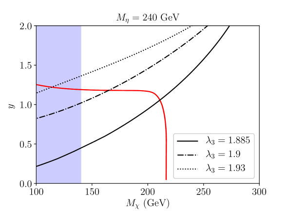
Figure 11: Overlap of strong phase transition and DM energy density in the $(M_{\chi},y)$-plane for $M_{\eta}=240$ GeV and $\lambda_{2}=1.25$. Black lines contour the $v_{3,{\rm c}}/\sqrt{T_{{\rm c},\phi}}=1$ for different values of $\lambda_{3}=\{1.885,1.9,1.93\}$. The red narrow band depicts the observed DM energy density which changes indiscernibly between the different values of $\lambda_{3}$. The blue shaded region is excluded by the collider searches, and we show the most stringent case due to the coupling to a muon ($M_{\chi}>140$ GeV). Unlike in other plots contouring $v_{3,{\rm c}}/\sqrt{T_{{\rm c},\phi}}$, the transition strength does not increase towards the upper left corner. The behaviour of such contours is more complicated in the $(M_{\chi},y)$-plane, which we do not visualise here to maintain clarity.

The second visualisation focuses on the $(M_{\chi},y)$-plane in fig. 11 at fixed $M_{\eta}=240$ GeV. The three black curves (solid, dash-dotted, dotted) contour $v_{3,{\rm c}}/\sqrt{T_{{\rm c},\phi}}=1$, that signal a strong phase transition, for three (slightly) different portal couplings $\lambda_{3}$. A large sensitivity to a small change of $\lambda_{3}$ at one-per-cent level in the $(M_{\chi},y)$-plane is clearly visible. This reflects the non-trivial behaviour in the complementary parameter space $(M_{\eta},\lambda_{3})$ upon changing the dark fermion mass and Yukawa coupling $y$ (cf. fig. 3).

The situation is rather the opposite for the dark matter energy density. In the same fig. 11, all three values of $\lambda_{3}$ collapse onto the red narrow band and correspond to $\Omega_{{\mbox{\tiny\rm{DM}}}}h^{2}|_{{\mbox{\scriptsize obs.}}}$. This is largely consistent with a per-cent change in scalar portal coupling, that can only slightly affect the annihilation cross section and the corresponding extraction of the energy density. Hence, in this complementary visualisation, one may appreciate how differently the first-order phase transition and DM energy density depend on the model parameters. We also included the experimental constraint on the DM mass $M_{\chi}>140$ GeV for the case of the coupling of $\chi$ and $\eta$ with a muon. This limit is most stringent for $M_{\eta}=240$ GeV among the three lepton flavours (see fig. 7). In this light, one can exclude the case $\lambda_{3}=1.93$ for the simultaneous event of a strong phase transition and the observed DM relic density. A similar analysis can be repeated for other choices of parameters, to explore possible values for portal couplings.

6 Conclusions and outlook

In this article, we investigated the coexistence of a strong electroweak phase transition and the observed dark matter abundance using state-of-the-art methodology for the combined analyses, in perturbation theory. The phase transition analysis is performed within the 3d EFT which includes complete NLO thermal resummations via dimensional reduction. For the dark matter energy density via freeze-out, we included the effect of thermal masses, Sommerfeld enhancement and bound-state effects.

The model considered in the article is a $t$-channel mediator dark matter model, that belongs to a next-to-minimal class of simplified models offering a rich phenomenology at collider, direct and indirect searches. This setup goes beyond the minimal option of a DM singlet scalar coupled to the SM Higgs boson. Concretely, the model features a dark matter Majorana fermion that is a singlet under the SM gauge group, and a scalar particle that mediates between the visible and dark matter sector. Gauge-invariant and renormalisable operators can be built from the Majorana DM fermion, the scalar mediator and the SM chiral fermions. We considered interactions with right-handed leptons. The scalar mediator can couple directly to the Higgs boson and, therefore, affect the electroweak phase transition. As the main result, our study discerns regions of parameters space where both a strong phase transition and the observed DM energy density allow for one another.

Quantitatively we find that a strong first-order phase transition can be realised for a complex scalar mass $150~{}{\rm GeV}\lesssim M_{\eta}\lesssim 340~{}{\rm GeV}$ and a scalar portal coupling $0.75\lesssim\lambda_{3}\lesssim 2.5$, in the limit of a decoupled DM fermion. Next, we assessed the effect of the Yukawa coupling and the fermionic degree of freedom. The overall effect on the FOPT diagram $(M_{\eta},\lambda_{3})$ is mild since the Majorana fermion does not interact directly with the SM Higgs boson. However, the interplay between the Yukawa coupling and the DM mass non-trivially changes the parameter space compatible with a first-order transition. Different combinations of $y$ and $M_{\chi}$ enlarge or narrow the region compatible with a FOPT.

For extracting the dark matter energy density, we focused on the freeze-out production mechanism. To find accurately the parameter space consistent with observations, one needs to include the effects of co-annihilations of the accompanying scalar mediator. For sufficiently small mass splittings, the scalar pair annihilations are relevant and we have included the processes that are induced by the interaction between the scalar $\eta$ and the SM Higgs boson. Moreover, since the scalar mediator interacts with the $Z$-boson and the photon, the pair annihilations are affected by non-perturbative effects, namely Sommerfeld enhancement and bound-state formation. The main contribution to both effects is due to the interaction between the scalar $\eta$ and the photon for masses $M_{\eta}\lesssim 1$ TeV. By combing the two effects, we find an impact on the DM energy density that ranges between 1–10% depending on the relative mass splitting $(M_{\eta}-M_{\chi})/M_{\chi}$ and the scalar portal coupling $\lambda_{3}$. We restricted the mass range $M_{\chi},M_{\eta}\lesssim 1$ TeV because larger values are not interesting for the EWPT. More importantly, this mass range maintains the phase transition and DM production as two separate events along the cosmological history, as the freeze-out temperature is below the critical temperature of the phase transition.

The main result of our study is shown in figs. 9 and 10. The overlapping region of a correct DM energy density and FOPT strongly depends on the Majorana fermion mass $M_{\chi}$ and the Yukawa coupling $y$. Upon increasing $M_{\chi}$, one has to also take larger values of $M_{\eta}$ (the DM model requires $M_{\chi}<M_{\eta}$), and hence the perturbative upper bound $M_{\eta}\lesssim 350$ GeV is soon saturated. The same holds when increasing the value of the Yukawa coupling to $y\approx 1$. We find that the value $y\simeq 0.1$ provides the lowest possible scalar masses. There is no effect in decreasing $y$ further since the DM energy density is governed by the scalar pair annihilations for the mass range of interest for $y\simeq 0.1$. When choosing the smallest DM fermion mass that avoids entirely the collider constrains, we find that the observed energy density and a strong electroweak phase transition can be realised in the present model for $140~{}{\rm GeV}<M_{\chi}\lesssim 300~{}{\rm GeV}$ ($180~{}{\rm GeV}<M_{\chi}\lesssim 300~{}{\rm GeV}$) for coupling to taus (muons). Moreover, one may look at the interplay between a FOPT and DM in the parameter space $(M_{\chi},y)$ in fig. 11. Here, a rather sharp difference on the dependence of the scalar portal coupling appears. While very slight changes in $\lambda_{3}$ sensibly change the $v_{c}/T_{{\mbox{\scriptsize c}},\phi}=1$ condition, they leave the DM energy density unaffected. Most importantly, the collider constraints can exclude values of $\lambda_{3}$ that allow for a strong EWPT.

The present analysis can be extended into various directions. First, the freeze-in production deserves attention in the light of null searches of WIMP-like DM particles. The DM could be merely interacting feebly with the visible sector and there could still exist compelling constraints for $t$-channel models from long-lived particles at colliders (in our case the lifetime of the produced $\eta$ would be long due to a tiny $y$). For the freeze-in mechanism, additional complexity in our investigation would be introduced by relaxing the assumption that both DM production and EWPT occurred as separate events in the thermal history of the universe. Thus, non-trivial cross influences of both events are conceivable but would require theoretical tools to extend to broader temperature ranges. Furthermore, different realisations of the present model where the Majorana fermion is coupled to a left-handed fermion are worth exploring as in e.g. [45, 19]. The corresponding mediator would then be charged under the ${\rm SU(2)}_{\mbox{\tiny\rm{L}}}$ gauge group.

Second, it is conceivable to implement the pipeline connecting the thermodynamics of a strong first-order phase transition with the production of a stochastic gravitational wave spectrum. Such an implementation can be realised within the 3d EFT to account for NLO thermal resummations as in [38, 36]. Furthermore, the EFT picture allows for consistently computing the bubble nucleation rate and nucleation temperature [143] as well as including higher order corrections [144, 145]. Such a computation goes beyond the scope of this article and is left for future studies. Nevertheless, we can expect that a strong enough GW signature for LISA-generation interferometers could be generated in a subregion of two-step phase transition regions – in analogy to a recent analysis [146].

Finally, we foresee a link between the simplified model approach for dark matter and exploring possible new-physics affecting the electroweak phase transitions. There has been extensive effort in classifying DM models, that exploit the Higgs portal as the main actor in connecting the visible to a dark sector (see e.g. reviews [147, 148]). A similar framework could help to estimate the effects on the EWPT due to new physics coupled to the SM Higgs boson. In the same spirit of a simplified model approach for DM, one can classify new-physics models depending on the particle that couples to the Higgs boson, such as scalars, gauge bosons, or fermions. The latter may share additional interactions with the SM degrees of freedom or with a dark sector or both. One may still capture the relevant effect on the thermodynamics of the phase transition once a minimal set of fields and couplings is given. This way, the impact on the EWPT can be assessed without necessarily relying on a fully-fledged UV theory, as we explored in our study.

Appendix A Dimensional reduction and thermal effective potential

This appendix collects renormalisation group equations (RGE), the matching relations of the model defined in eq. (2.1) to its dimensionally reduced three-dimensional effective theory in eq. (3.1), and the thermal effective potential computed within the EFT.

A.1 Renormalisation and one-loop beta functions

The renormalisation group equations listed below are associated with the parameters of the model in eq. (2.1) and encode their running with respect to the $\overline{\rm MS}$ renormalisation scale $\bar{\mu}$ via the beta functions. To this end, we use

$$t\equiv\ln\bar{\mu}^{2}\;,$$ (A.1)

and find at one-loop level

$$\partial_{t}g_{1}^{2} =\beta_{{\mbox{\tiny\rm{SM}}}}(g_{1}^{2})+\frac{1}{(4\pi)^{2}}\Big{(}\frac{1}{12}Y_{\eta}^{2}g_{1}^{4}\Big{)}\;,$$ (A.2)

$$\partial_{t}g_{2}^{2} =\beta_{{\mbox{\tiny\rm{SM}}}}(g_{2}^{2})\;,$$ (A.3)

$$\partial_{t}g_{\mbox{\tiny\rm{$Y$}}}^{2} =\beta_{{\mbox{\tiny\rm{SM}}}}(g_{\mbox{\tiny\rm{$Y$}}}^{2})\;,$$ (A.4)

$$\partial_{t}\mu_{\phi}^{2} =\beta_{{\mbox{\tiny\rm{SM}}}}(\mu^{2}_{\phi})+\frac{1}{(4\pi)^{2}}\Bigl{(}\lambda_{3}\mu_{\eta}^{2}\Bigr{)}\;,$$ (A.5)

$$\partial_{t}\mu_{\eta}^{2} =\frac{1}{(4\pi)^{2}}\Big{(}2\lambda_{3}\mu^{2}_{\phi}-2|y|^{2}\mu^{2}_{\chi}+\Bigl{(}4\lambda_{2}-\frac{3}{4}Y_{\eta}^{2}g_{1}^{2}+|y|^{2}\Bigr{)}\mu^{2}_{\eta}\Big{)}\;,$$ (A.6)

$$\partial_{t}\mu_{\chi}^{2} =\frac{1}{(4\pi)^{2}}|y|^{2}\mu_{\chi}^{2}\;,$$ (A.7)

$$\partial_{t}\lambda_{1} =\beta_{{\mbox{\tiny\rm{SM}}}}(\lambda_{1})+\frac{1}{(4\pi)^{2}}\Bigl{(}\frac{1}{2}\lambda_{3}^{2}\Bigr{)}\;,$$ (A.8)

$$\partial_{t}\lambda_{2} =\frac{1}{(4\pi)^{2}}\Big{(}\lambda_{3}^{2}+10\lambda_{2}^{2}-\frac{3}{2}Y_{\eta}^{2}g_{1}^{2}\lambda_{2}+\frac{3}{16}Y_{\eta}^{4}g_{1}^{4}+(2\lambda_{2}-|y|^{2})|y|^{2}\Big{)}\;,$$ (A.9)

$$\partial_{t}\lambda_{3} =\frac{1}{(4\pi)^{2}}\Big{(}\lambda_{3}\Big{[}2\lambda_{3}+4\lambda_{2}-\frac{3}{4}(3g_{2}^{2}+(Y_{\phi}^{2}+Y_{\eta}^{2})g_{1}^{2})+N_{\rm c}g_{\mbox{\tiny\rm{$Y$}}}^{2}+|y|^{2}+6\lambda_{1}\Big{]}$$

$$\hphantom{=\frac{1}{(4\pi)^{2}}\Big{(}}+\frac{3}{8}Y^{2}_{\eta}Y_{\phi}^{2}g_{1}^{4}\Big{)}\;,$$ (A.10)

$$\partial_{t}|y|^{2} =\frac{1}{(4\pi)^{2}}\Bigl{(}2|y|^{4}-\frac{3}{4}|y|^{2}g_{1}^{2}Y_{\eta}^{2}\Bigr{)}\;.$$ (A.11)

A generalisation of the beta function for $|y|$ can be found in [149]. The functions $\beta_{{\mbox{\tiny\rm{SM}}}}$ are pure SM contributions, that can be read e.g. from [70]. At the accuracy of a NLO dimensional reduction, the strong coupling $g_{\mbox{\scriptsize s}}$ merely enters the thermal mass for the Higgs doublet at two-loop order and can be fixed to $g_{\mbox{\scriptsize s}}(M_{\mbox{\tiny\rm{$Z$}}})=1.48409$ [150].

Background field dependent mass eigenvalues

Using the scalar field parameterisation in eq. (3.3), the mass eigenvalues in terms of generic background fields $v$ and $x$ read

$$M_{\mbox{\tiny\rm{$W$}}}^{2} =\frac{1}{4}g_{2}^{2}v^{2}\;,$$ (A.12)

$$M_{\pm}^{2} =\frac{1}{8}\biggl{(}(g_{2}^{2}+g_{1}^{2})v^{2}+Y_{\eta}^{2}g_{1}^{2}x^{2}$$

$$\hphantom{{}=\frac{1}{8}\biggl{(}(g_{2}^{2}+g_{1}^{2})v^{2}}\pm\sqrt{g_{2}^{4}v^{4}+2g_{2}^{2}g_{1}^{2}v^{2}(v^{2}-Y_{\eta}^{2}x^{2})+g_{1}^{4}(v^{2}+Y_{\eta}^{2}x^{2})^{2}}\biggr{)}\;,$$ (A.13)

for the gauge fields. The $W$-mass is double degenerate, and $M_{+}$($M_{-}$) is the eigenvalue for the $Z$-boson (photon) that reduces to the SM expressions for vanishing $x$. For scalars,

$$m_{\mbox{\tiny\rm{$G$}}}^{2} =\mu^{2}_{\phi}+\lambda_{1}v^{2}+\frac{1}{2}\lambda_{3}x^{2}\;,$$ (A.14)

$$m_{\mbox{\tiny\rm{$A$}}}^{2} =\mu^{2}_{\eta}+\lambda_{2}x^{2}+\frac{1}{2}\lambda_{3}v^{2}\;,$$ (A.15)

$$m^{2}_{\pm} =\frac{1}{2}(\mu^{2}_{\phi}+\mu^{2}_{\eta})+\Bigl{(}\frac{3}{2}\lambda_{1}+\frac{1}{4}\lambda_{3}\Bigr{)}v^{2}+\Bigl{(}\frac{3}{2}\lambda_{2}+\frac{1}{4}\lambda_{3}\Bigr{)}x^{2}$$

$$\pm\Bigl{(}(v^{4}+14v^{2}x^{2}+x^{4})\lambda_{3}^{2}+4\lambda_{3}(v^{2}-x^{2})(3\lambda_{1}v^{2}+3\lambda_{2}x^{2}-\mu_{\phi}^{2}+\mu_{\eta}^{2})$$

$$+4(3\lambda_{1}v^{2}+3\lambda_{2}x^{2}-\mu_{\phi}^{2}+\mu_{\eta}^{2})^{2}\Bigr{)}^{\frac{1}{2}}\;,$$ (A.16)

where the Goldstone mass eigenvalue $m_{\mbox{\tiny\rm{$G$}}}^{2}$ is triple degenerate, and the top quark has the mass eigenvalue

$$m^{2}_{t} =\frac{1}{2}g_{\mbox{\tiny\rm{$Y$}}}^{2}v^{2}\;.$$ (A.17)

For other SM fermions, the Yukawa couplings are assumed to vanish, as their effect is negligible for EWPT thermodynamics [64].

Relation of $\overline{\rm MS}$ and input parameters

At zero temperature, the vacuum-expectation-value for the singlet is assumed to vanish. As a result of setting the background field $x=0$, we identify $m_{\mbox{\tiny\rm{$A$}}}=m_{+}\equiv M_{\eta}$. The Goldstone mass eigenvalue vanishes at the electroweak minimum

$$v_{0}=\sqrt{\frac{4M_{\mbox{\tiny\rm{$W$}}}^{2}}{g^{2}_{0}}}\;,$$ (A.18)

where we install a shorthand notation $g^{2}_{0}\equiv 4\sqrt{2}G_{{\mbox{\scriptsize F}}}M_{\mbox{\tiny\rm{$W$}}}^{2}$, and the reduced Fermi constant $G_{{\mbox{\scriptsize F}}}=1.1663787\times 10^{-5}~{}{\rm GeV}^{-2}$. In terms of the masses

$$\bigl{\{}M_{\mbox{\tiny\rm{$W$}}},M_{\mbox{\tiny\rm{$Z$}}},M_{t}\bigr{\}}=\bigl{\{}80.379~{}{\rm GeV},91.1876~{}{\rm GeV},172.76~{}{\rm GeV}\bigr{\}}\;,$$

the gauge and Yukawa couplings are

$$g_{2}^{2} =g^{2}_{0}\;, g_{1}^{2} =g^{2}_{0}\Big{(}\frac{M_{\mbox{\tiny\rm{$Z$}}}^{2}}{M_{\mbox{\tiny\rm{$W$}}}^{2}}-1\Big{)}\;, g_{\mbox{\tiny\rm{$Y$}}}^{2} =\frac{1}{2}g^{2}_{0}\frac{M^{2}_{t}}{M_{\mbox{\tiny\rm{$W$}}}^{2}}\;.$$ (A.19)

By inverting the scalar mass eigenvalues, we get

$$\lambda_{1} =\frac{1}{2}\frac{M^{2}_{\phi}}{v^{2}_{0}}\;, \mu^{2}_{\phi} =-\frac{1}{2}M^{2}_{\phi}\;, \mu^{2}_{\eta} =M^{2}_{\eta}-\frac{1}{2}\lambda_{3}v^{2}_{0}\;.$$ (A.20)

Here, the Higgs mass $M_{\phi}=125.1$ GeV, $\lambda_{2}$, $\lambda_{3}$, and the unknown mass $M_{\eta}$ are treated as free input parameters. We assume that the Higgs is identified with the lighter eigenstate, i.e. $M^{2}_{\phi}=m^{2}_{-}$, and the singlet related states have identical masses $M^{2}_{\eta}\equiv m_{\mbox{\tiny\rm{$A$}}}^{2}=m^{2}_{+}$. The above relations are valid at LO, and receive loop corrections that could be included at one-loop, or NLO along the lines of [64, 71, 151, 66]. However, we do not consider these corrections here. The dark matter mass parameter has a trivial LO relation

$$\mu^{2}_{\chi}=M^{2}_{\chi}\;,$$ (A.21)

with its physical mass $M_{\chi}$.

For the tree-level potential ($V$) at zero temperature to be bounded from below, the parameters have to satisfy [152]

$$\lambda_{1},\lambda_{2}>0\;,\qquad\lambda_{3}+2\sqrt{\lambda_{1}\lambda_{2}}>0\;.$$ (A.22)

The Higgs and singlet phases are described by

$$(v,x)\stackrel{{\scriptstyle\text{Higgs}}}{{=}}\biggl{(}i\sqrt{\frac{\mu^{2}_{\phi}}{\lambda_{1}}},0\biggr{)}\;,\qquad(v,x)\stackrel{{\scriptstyle\text{singlet}}}{{=}}\biggl{(}0,i\sqrt{\frac{\mu^{2}_{\eta}}{\lambda_{2}}}\biggr{)}\;.$$ (A.23)

These solutions for the background fields extremise the tree-level potential, and we identify the Higgs phase as the zero-temperature electroweak minimum. There are also other solutions for extrema, that are not minima of the potential. For a two-variable function, the extremising condition for the minima is

$$\underbrace{\frac{\partial^{2}V}{\partial v^{2}}}_{>0}\frac{\partial^{2}V}{\partial x^{2}}-\Big{(}\frac{\partial^{2}V}{\partial v\partial x}\Big{)}^{2}>0\;.$$ (A.24)

If both Higgs and singlet minima coexist at the same parameter point, we require a global Higgs minimum.

A.2 Parameters of the 3d EFT

The effective parameters of the dimensionally reduced theory are collected below. Our independent computation here also agrees with the output of DRalgo [65]. To aid compactness, we define a shorthand notation

$$L_{b} \equiv 2\ln\Big{(}\frac{\mu}{T}\Big{)}-2\Big{(}\ln(4\pi)-{\gamma_{\mbox{\tiny\rm{E}}}}\Big{)}\;,\quad L_{f}\equiv L_{b}+4\ln 2\;,$$ (A.25)

$$c =\frac{1}{2}\Bigl{(}\ln\Big{(}\frac{8\pi}{9}\Big{)}+(\ln\zeta_{2})^{\prime}-2{\gamma_{\mbox{\tiny\rm{E}}}}\Bigr{)}\;,$$ (A.26)

where ${\gamma_{\mbox{\tiny\rm{E}}}}$ is the Euler-Mascheroni constant, $\zeta_{s}=\zeta(s)$ for $\mathop{\mbox{Re}}\,(s)>1$ is the Riemann zeta function, and $(\ln\zeta_{s})^{\prime}=\zeta^{\prime}(s)/\zeta(s)$. In the high-temperature expansion, and given that the number of fermion generations $n_{\rm f}=3$, the matching relations are

$$g_{1,3}^{2} =g_{1}^{2}T\bigg{[}1-\frac{g_{1}^{2}}{(4\pi)^{2}}\frac{1}{6}\Big{(}L_{b}\Big{[}Y_{\phi}^{2}+\frac{1}{2}Y_{\eta}^{2}\Big{]}+L_{f}Y_{{\mbox{\scriptsize 2f}}}\,n_{\rm f}\Big{)}\bigg{]}\;,$$ (A.27)

$$g_{2,3}^{2} =g_{2}^{2}T\bigg{[}1+\frac{g_{2}^{2}}{(4\pi)^{2}}\Big{(}\frac{43}{6}L_{b}+\frac{2}{3}-\frac{(N_{\rm c}+1)n_{\rm f}}{3}L_{f}\Big{)}\bigg{]}\;,$$ (A.28)

$$m_{{\mbox{\tiny\rm{D}}}{\mbox{\tiny\rm{1}}}}^{2} =\Big{(}m_{{\mbox{\tiny\rm{D}}}{\mbox{\tiny\rm{1}}}}^{2}\Big{)}_{{\mbox{\tiny\rm{SM}}}}+T^{2}g_{1}^{2}\bigg{[}\frac{1}{12}+\frac{1}{(4\pi)^{2}}\frac{\mu_{\eta}^{2}}{T^{2}}\bigg{]}Y_{\eta}^{2}$$

$$+\frac{T^{2}}{(4\pi)^{2}}g_{1}^{2}\bigg{[}-\bigg{(}\frac{L_{b}-7}{144}Y_{\eta}^{4}+\frac{L_{b}+2}{36}Y_{\phi}Y_{\eta}^{2}+\frac{(L_{b}+4L_{f}-2)Y_{{\mbox{\scriptsize 2f}}}Y_{\eta}^{2}}{288}n_{\rm f}\bigg{)}g_{1}^{2}$$

$$\hphantom{{}+\frac{T^{2}}{(4\pi)^{2}}g_{1}^{2}\bigg{[}}+\frac{1}{6}\lambda_{3}\big{[}Y_{\phi}^{2}+Y_{\eta}^{2}\big{]}+\frac{1}{3}\lambda_{2}Y_{\eta}^{2}-\frac{Y_{\eta}^{2}}{24}|y|^{2}\bigg{]}\;,$$ (A.29)

$$m_{{\mbox{\tiny\rm{D}}}{\mbox{\tiny\rm{2}}}}^{2} =\Big{(}m_{{\mbox{\tiny\rm{D}}}{\mbox{\tiny\rm{2}}}}^{2}\Big{)}_{{\mbox{\tiny\rm{SM}}}}+\frac{T^{2}}{(4\pi)^{2}}\frac{1}{6}g_{2}^{2}\lambda_{3}\;,$$ (A.30)

$$\mu_{\phi,3}^{2} =\Big{(}\mu^{2}_{\phi,3}\Big{)}_{{\mbox{\tiny\rm{SM}}}}+\frac{T^{2}}{12}\lambda_{3}-\frac{L_{b}}{(4\pi)^{2}}\lambda_{3}\mu^{2}_{\eta}$$

$$+T^{2}\frac{Y_{\eta}^{2}}{(4\pi)^{2}}\Big{(}\frac{5}{288}\,g_{1}^{4}\,Y_{\phi}^{2}+\frac{1}{24}\,g_{1}^{2}\,\lambda_{3}\Big{)}+T^{2}L_{f}\frac{\lambda_{3}}{(4\pi)^{2}}\frac{1}{12}\Bigl{(}\frac{1}{2}\,|y|^{2}-N_{\rm c}\,g_{\mbox{\tiny\rm{$Y$}}}^{2}\Bigr{)}$$

$$-T^{2}L_{b}\frac{1}{(4\pi)^{2}}\bigg{(}\frac{7}{192}\,g_{1}^{4}\,Y_{\eta}^{2}Y_{\phi}^{2}$$

$$\hphantom{-T^{2}L_{b}\frac{1}{(4\pi)^{2}}\bigg{(}}+\lambda_{3}\Big{(}\frac{5}{12}\,\lambda_{3}+\frac{\lambda_{1}}{2}+\frac{\lambda_{2}}{3}\,+\frac{1}{8}\,|y|^{2}-\frac{1}{16}g_{1}^{2}\bigl{(}Y_{\phi}^{2}+Y_{\eta}^{2}\bigr{)}-\frac{3}{16}\,g_{2}^{2}\Big{)}\bigg{)}$$

$$+T^{2}\,\Big{(}c+\ln\Big{(}\frac{3T}{\bar{\mu}_{{\mbox{\tiny\rm{3d}}}}}\Big{)}\Big{)}\frac{1}{(4\pi)^{2}}\bigg{(}-\lambda_{3}^{2}+\frac{1}{2}\,g_{1}^{2}\,\lambda_{3}\,Y_{\eta}^{2}-\frac{1}{16}\,g_{1}^{4}\,Y_{\eta}^{2}Y_{\phi}^{2}\bigg{)}\;,$$ (A.31)

$$\lambda_{1,3} =\Big{(}\lambda_{1,3}\Big{)}_{{\mbox{\tiny\rm{SM}}}}+T\bigg{[}-\frac{L_{b}}{(4\pi)^{2}}\frac{1}{2}\lambda_{3}^{2}\bigg{]}\;,$$ (A.32)

where $N_{\rm c}=3$ is the number of colours. The momentum-dependent parts of the renormalised 2-point correlation functions yield

$$\hat{\Pi}^{\prime}_{A_{0}^{a}A_{0}^{b}} =\frac{g_{2}^{2}}{(4\pi)^{2}}\bigg{(}3+\frac{(N_{\rm c}+1)}{3}n_{\rm f}(L_{f}-1)+\Big{(}\xi_{2}-\frac{25}{6}\Big{)}L_{b}-2\xi_{2}\bigg{)}\;,$$ (A.33)

$$\hat{\Pi}^{\prime}_{A_{r}^{a}A_{s}^{b}} =\frac{g_{2}^{2}}{(4\pi)^{2}}\bigg{(}-\frac{2}{3}+\frac{(N_{\rm c}+1)}{3}n_{\rm f}L_{f}+\Big{(}\xi_{2}-\frac{25}{6}\Big{)}L_{b}\bigg{)}\;,$$ (A.34)

$$\hat{\Pi}^{\prime}_{B_{0}B_{0}} =\frac{g_{1}^{2}}{(4\pi)^{2}}\frac{1}{6}\Big{(}\Big{[}Y_{\phi}^{2}+\frac{1}{2}Y_{\eta}^{2}\Big{]}(L_{b}+2)+Y_{{\mbox{\scriptsize 2f}}}\,n_{\rm f}(L_{f}-1)\Big{)}\;,$$ (A.35)

$$\hat{\Pi}^{\prime}_{B_{r}B_{s}} =\frac{g_{1}^{2}}{(4\pi)^{2}}\frac{1}{6}\Big{(}\Big{[}Y_{\phi}^{2}+\frac{1}{2}Y_{\eta}^{2}\Big{]}L_{b}+Y_{{\mbox{\scriptsize 2f}}}\,n_{\rm f}L_{f}\Big{)}\;,$$ (A.36)

$$\hat{\Pi}^{\prime}_{\phi^{\dagger}\phi} =\frac{1}{(4\pi)^{2}}\bigg{(}-\frac{L_{b}}{4}\Big{(}3(3-\xi_{2})g_{2}^{2}+(3-\xi_{1})g_{1}^{2}Y_{\phi}^{2}\Big{)}+N_{\rm c}L_{f}g_{\mbox{\tiny\rm{$Y$}}}^{2}\bigg{)}\;,$$ (A.37)

$$\hat{\Pi}^{\prime}_{\eta^{\dagger}\eta} =\frac{1}{(4\pi)^{2}}\bigg{(}-\frac{L_{b}}{4}(3-\xi_{1})g_{1}^{2}Y_{\eta}^{2}+L_{f}|y|^{2}\bigg{)}\;,$$ (A.38)

where $\xi_{1}$ is the ${\rm U(1)}_{\mbox{\tiny\rm{Y}}}$ and $\xi_{2}$ is the ${\rm SU(2)}_{\mbox{\tiny\rm{L}}}$ gauge-fixing parameter. The remaining matching relations for the thermal mass of the complex ${\rm SU(2)}_{\mbox{\tiny\rm{L}}}$ singlet and its quartic couplings take the form

$$\mu_{\eta,3}^{2} =\mu^{2}_{\eta}+T^{2}\Big{(}\frac{1}{6}\lambda_{3}+\frac{1}{3}\lambda_{2}+\frac{Y_{\eta}^{2}}{16}g_{1}^{2}+\frac{1}{12}|y|^{2}\Big{)}$$

$$+\frac{1}{(4\pi)^{2}}\Big{(}L_{f}(2\mu_{\chi}^{2}-\mu_{\eta}^{2})|y|^{2}-L_{b}\Big{(}2\mu^{2}_{\phi}\lambda_{3}+\mu_{\eta}^{2}\Big{[}4\lambda_{2}-\frac{3}{4}g_{1}^{2}Y_{\eta}^{2}\Big{]}\Big{)}\Big{)}$$

$$+T^{2}\frac{1}{(4\pi)^{2}}\bigg{(}-\frac{g_{1}^{4}}{72}Y_{\eta}^{2}\Bigl{(}Y_{\eta}^{2}-\frac{5}{2}\,Y_{\phi}^{2}-\frac{1}{4}\,n_{\rm f}\,Y_{{\mbox{\scriptsize 2f}}}\Bigr{)}+\frac{1}{6}\,g_{1}^{2}\Bigl{(}\lambda_{2}\,Y_{\eta}^{2}+\frac{1}{2}\,\lambda_{3}\,Y_{\phi}^{2}\Bigr{)}$$

$$\hphantom{{}+T^{2}\frac{1}{(4\pi)^{2}}\bigg{(}}+\frac{1}{4}\,g_{2}^{2}\,\lambda_{3}-\frac{1}{48}|y|^{2}\,g_{1}^{2}\,Y_{e}^{2}\bigg{)}$$

$$+T^{2}L_{b}\frac{1}{(4\pi)^{2}}\bigg{(}-\frac{g_{1}^{4}}{96}Y_{\eta}^{2}\Big{(}\frac{13}{2}\,Y_{\eta}^{2}+7Y_{\phi}^{2}+\frac{3}{2}\,n_{\rm f}Y_{{\mbox{\scriptsize 2f}}}\Big{)}$$

$$\hphantom{{}+T^{2}L_{b}\frac{1}{(4\pi)^{2}}\bigg{(}}+\lambda_{3}\Big{(}-\frac{2}{3}\bigl{(}\lambda_{2}+\lambda_{3}\bigr{)}-\lambda_{1}+\frac{1}{8}\,g_{1}^{2}\bigl{(}Y_{\eta}^{2}+Y_{\phi}^{2}\bigr{)}+\frac{3}{8}\,g_{2}^{2}-\frac{N_{\rm c}}{4}g_{\mbox{\tiny\rm{$Y$}}}^{2}\Big{)}$$

$$\hphantom{{}+T^{2}L_{b}\frac{1}{(4\pi)^{2}}\bigg{(}}-\lambda_{2}\Bigl{(}\frac{10}{3}\lambda_{2}-\frac{1}{2}g_{1}^{2}\,Y_{\eta}^{2}+\frac{1}{2}|y|^{2}\Bigr{)}+\frac{1}{12}\,|y|^{4}+\frac{1}{96}\bigl{(}6Y_{\eta}^{2}+Y_{e}^{2}\bigr{)}|y|^{2}\,g_{1}^{2}\bigg{)}$$

$$+T^{2}L_{f}\frac{1}{(4\pi)^{2}}\bigg{(}\frac{1}{192}\,n_{\rm f}\,g_{1}^{4}\,Y_{\eta}^{2}Y_{{\mbox{\scriptsize 2f}}}-\frac{1}{96}\bigl{(}6Y_{\eta}^{2}-5Y_{e}^{2}\bigr{)}|y|^{2}\,g_{1}^{2}$$

$$\hphantom{{}+T^{2}L_{f}\frac{1}{(4\pi)^{2}}\bigg{(}}+\frac{N_{\rm c}}{12}g_{\mbox{\tiny\rm{$Y$}}}^{2}\,\lambda_{3}-\frac{1}{6}|y|^{2}\bigl{(}\lambda_{2}+\lambda_{3}\bigr{)}+\frac{1}{12}\,|y|^{4}\bigg{)}$$

$$+T^{2}\,\Big{(}c+\ln\Big{(}\frac{3T}{\bar{\mu}_{{\mbox{\tiny\rm{3d}}}}}\Big{)}\Big{)}\frac{1}{(4\pi)^{2}}\bigg{(}-\frac{3}{8}\,g_{1}^{4}\,Y_{\eta}^{4}-\frac{1}{8}\,g_{1}^{4}\,Y_{\eta}^{2}\,Y_{\phi}^{2}+g_{1}^{2}\bigl{(}\lambda_{3}\,Y_{\phi}^{2}+2\lambda_{2}\,Y_{\eta}^{2}\bigr{)}$$

$$\hphantom{{}+T^{2}\,\Big{(}c+\ln\Big{(}\frac{3T}{\bar{\mu}_{{\mbox{\tiny\rm{3d}}}}}\Big{)}\Big{)}\frac{1}{(4\pi)^{2}}\bigg{(}}-2\lambda_{3}^{2}-8\lambda_{2}^{2}+3g_{2}^{2}\,\lambda_{3}\bigg{)}\;,$$ (A.39)

$$\lambda_{2,3} =T\bigg{[}\lambda_{2}+\frac{1}{(4\pi)^{2}}\bigg{(}\frac{Y_{\eta}^{4}}{8}g_{1}^{4}+L_{f}\Big{(}|y|^{2}-2\lambda_{2}\Big{)}|y|^{2}$$

$$\hphantom{{}=T\bigg{[}\lambda_{2}+\frac{1}{(4\pi)^{2}}\bigg{(}\frac{Y_{\eta}^{4}}{8}g_{1}^{4}}-L_{b}\Big{(}\lambda_{3}^{2}+10\lambda_{2}^{2}+\frac{3}{16}Y_{\eta}^{4}g_{1}^{4}-\frac{3}{2}Y_{\eta}^{2}g_{1}^{2}\lambda_{2}\Big{)}\bigg{)}\bigg{]}\;,$$ (A.40)

$$\lambda_{3,3} =T\bigg{[}\lambda_{3}+\frac{1}{(4\pi)^{2}}\bigg{(}\frac{Y_{\eta}^{2}Y_{\phi}^{2}}{4}g_{1}^{4}-L_{b}\Big{(}2\lambda_{3}^{2}+4\lambda_{3}\lambda_{2}+\frac{3}{8}Y_{\eta}^{2}Y_{\phi}^{2}g_{1}^{4}+6\lambda_{1}\lambda_{3}$$

$$\hphantom{=T\bigg{[}\lambda_{3}+\frac{1}{(4\pi)^{2}}\bigg{(}}-\frac{3}{4}g_{1}^{2}\lambda_{3}(Y_{\phi}^{2}+Y_{\eta}^{2})-\frac{9}{4}g_{2}^{2}\lambda_{3}\Big{)}-L_{f}\lambda_{3}\big{(}N_{\rm c}g_{\mbox{\tiny\rm{$Y$}}}^{2}+|y|^{2}\big{)}\bigg{)}\bigg{]}\;,$$ (A.41)

$$h_{3}^{\prime} =\frac{g_{1}^{2}T}{2}\bigg{[}Y_{\phi}^{2}+\frac{1}{(4\pi)^{2}}\bigg{(}\frac{3g^{2}}{2}Y_{\phi}^{2}-\frac{1}{12}\Big{(}2(L_{b}-1)Y_{\phi}^{2}+(L_{b}+2)Y_{\eta}^{2}+2(L_{f}-1)Y_{{\mbox{\scriptsize 2f}}}\,n_{\rm f}\Big{)}g_{1}^{2}Y_{\phi}^{2}$$

$$\hphantom{{}=\frac{g_{1}^{2}T}{4}\bigg{[}Y_{\phi}^{2}}-2(Y_{q}^{2}+Y_{u}^{2})N_{\rm c}g_{\mbox{\tiny\rm{$Y$}}}^{2}+12\lambda_{1}Y_{\phi}^{2}+2\lambda_{3}Y_{\eta}^{2}\bigg{)}\bigg{]}\;,$$ (A.42)

$$\rho_{3}^{\prime} =\frac{g_{1}^{2}T}{2}\bigg{[}Y_{\eta}^{2}+\frac{1}{(4\pi)^{2}}\bigg{(}\frac{1}{12}\Big{(}2(L_{b}+2)Y_{\phi}^{2}+(L_{b}-4)Y_{\eta}^{2}-2(L_{f}-1)Y_{{\mbox{\scriptsize 2f}}}\,n_{\rm f}\Big{)}g_{1}^{2}Y_{\eta}^{2}$$

$$\hphantom{{}=\frac{g_{1}^{2}T}{2}\bigg{[}Y_{\eta}^{2}}+\big{(}(Y_{e}^{2}-Y_{\eta}^{2})L_{f}-2Y_{e}^{2}\big{)}|y|^{2}+8\lambda_{2}Y_{\eta}^{2}+4\lambda_{3}Y_{\phi}^{2}\bigg{)}\bigg{]}\;,$$ (A.43)

for which we abbreviate recurring sums as

$$\sum_{f}Y_{{\mbox{\scriptsize f}}}^{4}\equiv Y_{{\mbox{\scriptsize 4f}}} =\Bigl{[}(Y_{e}^{4}+2Y_{\ell}^{4})+N_{\rm c}(Y_{u}^{4}+Y_{d}^{4}+2Y_{q}^{4})\Bigr{]}=\frac{2}{81}(729+137N_{\rm c})=\frac{760}{27}\;,$$ (A.44)

$$\sum_{f}Y_{{\mbox{\scriptsize f}}}^{2}\equiv Y_{{\mbox{\scriptsize 2f}}} =\Bigl{[}(Y_{e}^{2}+2Y_{\ell}^{2})+N_{\rm c}(Y_{u}^{2}+Y_{d}^{2}+2Y_{q}^{2})\Bigr{]}=\frac{2}{9}(27+11N_{\rm c})=\frac{40}{3}\;,$$ (A.45)

with the corresponding hypercharges $Y_{e},Y_{\ell},Y_{u},Y_{d},Y_{q}$ collected in [70].

The novel ultrasoft matching relations besides from the SM [70] are

$$\bar{\mu}_{\eta,3}^{2} =\mu_{\eta,3}^{2}-\frac{1}{8\pi}\rho_{3}^{\prime}m_{{\mbox{\tiny\rm{D}}}{\mbox{\tiny\rm{1}}}}\;,$$ (A.46)

$$\bar{\lambda}_{2,3} =\lambda_{2,3}-\frac{1}{32\pi}\frac{\rho_{3}^{\prime 2}}{m_{{\mbox{\tiny\rm{D}}}{\mbox{\tiny\rm{1}}}}}\;,$$ (A.47)

$$\bar{\lambda}_{3,3} =\lambda_{3,3}-\frac{1}{16\pi}\frac{h_{3}^{\prime}\rho_{3}^{\prime}}{m_{{\mbox{\tiny\rm{D}}}{\mbox{\tiny\rm{1}}}}}\;.$$ (A.48)

One-loop thermal functions for the Majorana fermion

The assumption of high-temperature expansion is relaxed for the Majorana fermion mass parameter, at one-loop level. A full two-loop treatment is relegated to future work and would be required for full NLO dimensional reduction.

The one-loop fermionic master integrals can be recast into a vacuum part and a thermal integral $\widetilde{Z}^{{\mbox{\tiny\rm{$T$}}}}$ that can be evaluated numerically

$$\widetilde{Z}_{s;i}^{\alpha} ={\hbox{$\sum$}\!\!\!\!\!\!\!\int\,}_{\!\!\!\!\raise-2.71246pt\hbox{$\scriptstyle{\{P\}}$}}\frac{p_{n}^{\alpha}}{[P^{2}+m_{i}^{2}]^{s}}\;, \widetilde{Z}_{s;i}^{0}=\widetilde{Z}_{s;i} ={\hbox{$\sum$}\!\!\!\!\!\!\!\int\,}_{\!\!\!\!\raise-2.71246pt\hbox{$\scriptstyle{\{P\}}$}}\frac{1}{[P^{2}+m_{i}^{2}]^{s}}=I_{s;i}^{4}+\widetilde{Z}_{s;i}^{{\mbox{\tiny\rm{$T$}}}}\;,$$ (A.49)

where the four-momenta $P\equiv(p_{n},{\bf p})$ and $p_{n}$ is a Matsubara frequency. The curly brackets indicate the fermionic nature of the thermal sums and that $p_{n}$ is fermionic, i.e. $p_{n}=(2n+1)\pi T$ with $n\in\mathbb{Z}$. The $d$-dimensional integral measure is

$$\int_{{\bf p}}\equiv\int\frac{{\rm d}^{d}{\bf p}}{(2\pi)^{d}}=\frac{2}{(4\pi)^{2}\Gamma(\frac{d}{2})}\int_{0}^{\infty}{\rm d}p\,p^{d-1}\;.$$ (A.50)

The term $I_{s;i}^{4}$ is the 4d vacuum integral in $d\to d+1=4-2\epsilon$

$$I_{s;i}^{d}\equiv\Bigl{(}\frac{\bar{\mu}^{2}e^{\gamma_{\mbox{\tiny\rm{E}}}}}{4\pi}\Bigr{)}^{\epsilon}\int_{{\bf p}}\frac{1}{(P^{2}+m_{i}^{2})^{\alpha}}=\Bigl{(}\frac{\bar{\mu}^{2}e^{\gamma_{\mbox{\tiny\rm{E}}}}}{4\pi}\Bigr{)}^{\epsilon}\frac{[m_{i}^{2}]^{\frac{d}{2}-s}}{(4\pi)^{\frac{d}{2}}}\frac{\Gamma\bigl{(}s-\frac{d}{2}\bigr{)}}{\Gamma(s)}\;.$$ (A.51)

The high-temperature expansion ($m_{i}\ll T$) of the master integrals that contribute to the fermionic sector of the matching relations at one-loop level in $d=3-2\epsilon$ is

$$\widetilde{Z}_{1;i} = I_{1;i}^{4}+\widetilde{Z}_{1;i}^{{\mbox{\tiny\rm{$T$}}}}$$ (A.52)

$$= -\frac{m_{i}^{2}}{(4\pi)^{2}}\Bigl{[}\frac{1}{\epsilon}+\ln\Bigl{(}\frac{\bar{\mu}^{2}}{m_{i}^{2}}\Bigr{)}+1\Bigr{]}+\widetilde{Z}_{1;i}^{{\mbox{\tiny\rm{$T$}}}}+\mathcal{O}(\epsilon)$$

$$\stackrel{{\scriptstyle m_{i}\ll T}}{{=}} -\frac{T^{2}}{24}-\frac{m_{i}^{2}}{(4\pi)^{2}}\Bigl{[}\frac{1}{\epsilon}+L_{f}\Bigr{]}+\mathcal{O}\Bigl{(}\frac{m_{i}^{4}}{T^{2}},\epsilon\Bigr{)}\;,$$

$$\widetilde{Z}_{2;i} = I_{2;i}^{4}+\widetilde{Z}_{2;i}^{{\mbox{\tiny\rm{$T$}}}}$$ (A.53)

$$= \frac{1}{(4\pi)^{2}}\Bigl{[}\frac{1}{\epsilon}+\ln\Bigl{(}\frac{\bar{\mu}^{2}}{m_{i}^{2}}\Bigr{)}\Bigr{]}+\widetilde{Z}_{2;i}^{{\mbox{\tiny\rm{$T$}}}}+\mathcal{O}(\epsilon)$$

$$\stackrel{{\scriptstyle m_{i}\ll T}}{{=}} \frac{1}{(4\pi)^{2}}\Bigl{[}\frac{1}{\epsilon}+L_{f}\Bigr{]}+\mathcal{O}\Bigl{(}\frac{m_{i}^{2}}{T^{2}},\epsilon\Bigr{)}\;,$$

$$\widetilde{Z}_{1;i}^{2} = -\frac{m_{i}^{2}}{d+1}I_{1;i}^{4}-\widetilde{Z}_{1;i}^{2,{\mbox{\tiny\rm{$T$}}}}-m_{i}^{2}\widetilde{Z}_{1;i}^{{\mbox{\tiny\rm{$T$}}}}$$ (A.54)

$$= \frac{m_{i}^{4}}{4(4\pi)^{2}}\Bigl{[}\frac{1}{\epsilon}+\ln\Bigl{(}\frac{\bar{\mu}^{2}}{m_{i}^{2}}\Bigr{)}+\frac{3}{2}\Bigr{]}-\widetilde{Z}_{1;i}^{2,{\mbox{\tiny\rm{$T$}}}}+\mathcal{O}(\epsilon)$$

$$\stackrel{{\scriptstyle m_{i}\ll T}}{{=}} \frac{7(4\pi)^{2}}{3840}T^{4}-\frac{T^{2}m_{i}^{2}}{48}+\frac{m_{i}^{4}}{4(4\pi)^{2}}\Bigl{[}\frac{1}{\epsilon}+L_{f}+2\Bigr{]}+\mathcal{O}\Bigl{(}\frac{m_{i}^{6}}{T^{2}},\epsilon\Bigr{)}\;,$$

where the explicit fermionic thermal integrals up to $\mathcal{O}(\epsilon^{0})$ are

$$\widetilde{Z}_{1;i}^{{\mbox{\tiny\rm{$T$}}}} =-\int_{{\bf p}}\frac{n_{\mbox{\tiny\rm{F}}}(E_{p,i})}{E_{p,i}}\;,$$ (A.55)

$$\widetilde{Z}_{2;i}^{{\mbox{\tiny\rm{$T$}}}} =-\frac{1}{2}\int_{{\bf p}}\frac{n_{\mbox{\tiny\rm{F}}}(E_{p,i})}{p^{2}E_{p,i}}\;,$$ (A.56)

$$\widetilde{Z}_{1;i}^{2,{\mbox{\tiny\rm{$T$}}}} =-\int_{{\bf p}}\frac{p^{2}n_{\mbox{\tiny\rm{F}}}(E_{p,i})}{E_{p,i}}\;,$$ (A.57)

with $E_{p,i}\equiv\sqrt{p^{2}+m_{i}^{2}}$, $m_{i}$ a general mass, and the Fermi distribution function $n_{\mbox{\tiny\rm{F}}}(E)\equiv 1/[\mbox{exp}(E/T)+1]$.

Below we give the corresponding Majorana fermionic sector of the dimensional reduction matching relations. Therein the full one-loop dependence on the thermal integrals for the Majorana fermion $\widetilde{Z}_{s;\chi}^{\alpha,{\mbox{\tiny\rm{$T$}}}}$ is installed:

$$\hat{\Pi}^{\prime}_{\eta^{\dagger}\eta} \supset-|y|^{2}\Bigl{[}\frac{2}{\mu_{\chi}^{2}}\widetilde{Z}_{1;\chi}^{{\mbox{\tiny\rm{$T$}}}}+\frac{4}{3}\frac{1}{\mu_{\chi}^{4}}\Bigl{(}\widetilde{Z}_{1;\chi}^{2,{\mbox{\tiny\rm{$T$}}}}-\widetilde{Z}_{1;0}^{2,{\mbox{\tiny\rm{$T$}}}}\Bigr{)}-\frac{1}{(4\pi)^{2}}\Bigl{(}\ln\Bigl{(}\frac{\bar{\mu}^{2}}{\mu_{\chi}^{2}}\Bigr{)}+\frac{1}{2}\Bigr{)}\Bigr{]}\;,$$ (A.58)

$$\mu_{\eta,3}^{2} \supset-|y|^{2}\Bigl{[}2\widetilde{Z}_{1;\chi}^{{\mbox{\tiny\rm{$T$}}}}\Bigl{(}1-\frac{\mu_{\eta}^{2}}{\mu_{\chi}^{2}}\Bigr{)}-\frac{4}{3}\frac{\mu_{\eta}^{2}}{\mu_{\chi}^{4}}\Big{(}\widetilde{Z}_{1;\chi}^{2,{\mbox{\tiny\rm{$T$}}}}-\widetilde{Z}_{1;0}^{2,{\mbox{\tiny\rm{$T$}}}}\Bigr{)}$$

$$\hphantom{{}\supset-|y|^{2}\Bigl{[}2\widetilde{Z}_{1;\chi}^{{\mbox{\tiny\rm{$T$}}}}\Bigl{(}1-\frac{\mu_{\eta}^{2}}{\mu_{\chi}^{2}}\Bigr{)}}-\frac{\mu_{\chi}^{2}}{(4\pi)^{2}}\Bigl{(}\ln\Bigl{(}\frac{\bar{\mu}^{2}}{\mu_{\chi}^{2}}\Bigr{)}\Bigl{(}2-\frac{\mu_{\eta}^{2}}{\mu_{\chi}^{2}}\Bigr{)}+2-\frac{1}{2}\frac{\mu_{\eta}^{2}}{\mu_{\chi}^{2}}\Bigr{)}\Bigr{]}\;,$$ (A.59)

$$\lambda_{2,3} \supset T|y|^{4}\Bigl{[}\widetilde{Z}_{2;\chi}^{{\mbox{\tiny\rm{$T$}}}}+\frac{1}{(4\pi)^{2}}\ln\Bigl{(}\frac{\bar{\mu}^{2}}{\mu_{\chi}^{2}}\Bigr{)}\Bigr{]}$$

$$+2T|y|^{2}\lambda_{2}\Bigl{[}\frac{2}{\mu_{\chi}^{2}}\widetilde{Z}_{1;\chi}^{{\mbox{\tiny\rm{$T$}}}}+\frac{4}{3}\frac{1}{\mu_{\chi}^{4}}\Bigl{(}\widetilde{Z}_{1;\chi}^{2,{\mbox{\tiny\rm{$T$}}}}-\widetilde{Z}_{1;0}^{2,{\mbox{\tiny\rm{$T$}}}}\Bigr{)}-\frac{1}{(4\pi)^{2}}\Bigl{(}\ln\Bigl{(}\frac{\bar{\mu}^{2}}{\mu_{\chi}^{2}}\Bigr{)}+\frac{1}{2}\Bigr{)}\Bigr{]}\;,$$ (A.60)

$$\lambda_{3,3} \supset T|y|^{2}\lambda_{3}\Bigl{[}\frac{2}{\mu_{\chi}^{2}}\widetilde{Z}_{1;\chi}^{{\mbox{\tiny\rm{$T$}}}}+\frac{4}{3}\frac{1}{\mu_{\chi}^{4}}\Bigl{(}\widetilde{Z}_{1;\chi}^{2,{\mbox{\tiny\rm{$T$}}}}-\widetilde{Z}_{1;0}^{2,{\mbox{\tiny\rm{$T$}}}}\Bigr{)}-\frac{1}{(4\pi)^{2}}\Bigl{(}\ln\Bigl{(}\frac{\bar{\mu}^{2}}{\mu_{\chi}^{2}}\Bigr{)}+\frac{1}{2}\Bigr{)}\Bigr{]}\;,$$ (A.61)

$$\rho_{3}^{\prime} \supset-\frac{g_{1}^{2}|y|^{2}T}{2}\bigg{[}(Y_{e}^{2}-Y_{\eta}^{2})\Bigl{[}\frac{2}{\mu_{\chi}^{2}}\widetilde{Z}_{1;\chi}^{{\mbox{\tiny\rm{$T$}}}}+\frac{4}{3}\frac{1}{\mu_{\chi}^{4}}\Bigl{(}\widetilde{Z}_{1;\chi}^{2,{\mbox{\tiny\rm{$T$}}}}-\widetilde{Z}_{1;0}^{2,{\mbox{\tiny\rm{$T$}}}}\Bigr{)}-\frac{1}{(4\pi)^{2}}\Bigl{(}\ln\Bigl{(}\frac{\bar{\mu}^{2}}{\mu_{\chi}^{2}}\Bigr{)}+\frac{1}{2}\Bigr{)}\Bigr{]}$$

$$\hphantom{{}\supset\frac{g_{1}^{2}|y|^{2}T}{2}\bigg{[}}+\frac{2Y_{e}^{2}}{(4\pi)^{2}}\bigg{]}\;.$$ (A.62)

Here, $\widetilde{Z}_{s;0}^{\alpha,{\mbox{\tiny\rm{$T$}}}}$ is the zero-mass version of the corresponding thermal integral. In the limit $\mu_{\chi}\ll T$, we recover the matching relations as stated in the beginning of appendix A.2. One subtlety is the vanishing $\widetilde{Z}_{1;\chi}^{{\mbox{\tiny\rm{$T$}}}}$ term in eq. (A.2) in the limit $\mu_{\chi}\to\mu_{\eta}$. In that case, the high-temperature LO term $\frac{T^{2}|y|^{2}}{12}$ is produced from the momentum-dependent part of the $\eta$ correlator. This is a NLO contribution. Since LO and NLO are then of the same order, $\mu_{\chi}$ has to be at least soft or parametrically larger than a soft $\mu_{\eta}$ for a high-temperature expansion to be valid.

For fig. 3, we verified that there is no qualitative difference for the $v_{3,{\rm c}}/\sqrt{T_{{\rm c},\phi}}$ contours whether using dimensional reduction matching relations with a generic $\mu_{\chi}$ or a soft $\mu_{\chi}\sim gT$ with high-temperature expansion. However, using the high-temperature expansion could compromise the accuracy for large physical $M_{\chi}$ when determining the phase transition thermodynamics – such as the phase transition strength and inverse duration (cf. eg. [38]). We leave such an investigation for future work.

Thermal effective potential within 3d EFT

The effective potential at one-loop order within the 3d EFT reads

$$V^{{\mbox{\scriptsize 3d}}}_{{\mbox{\scriptsize eff}}} =V_{{\mbox{\scriptsize tree}}}+V_{{\mbox{\scriptsize 1-loop}}}\;.$$ (A.63)

At tree-level

$$V_{{\mbox{\scriptsize tree}}} =\frac{1}{2}\mu^{2}_{\phi,3}v^{2}_{3}+\frac{1}{2}\mu^{2}_{\eta,3}x^{2}_{3}+\frac{1}{4}\lambda_{1,3}v^{4}_{3}+\frac{1}{4}\lambda_{2,3}x^{4}_{3}+\frac{1}{4}\lambda_{3,3}v^{2}_{3}x^{2}_{3}\;.$$ (A.64)

At one-loop level, the effective potential can be written in terms of the master integral in general dimensions and explicit $d=3-2\epsilon$ dimensions

$$J_{d}(m^{2}) \equiv\frac{1}{2}\int_{{\bf p}}\ln(p^{2}+m^{2})=-\frac{1}{2}\Big{(}\frac{\bar{\mu}_{{\mbox{\tiny\rm{3d}}}}^{2}e^{\gamma_{\mbox{\tiny\rm{E}}}}}{4\pi}\Big{)}^{\epsilon}\frac{[m^{2}]^{\frac{d}{2}}}{(4\pi)^{\frac{d}{2}}}\frac{\Gamma(-\frac{d}{2})}{\Gamma(1)}\;,$$ (A.65)

$$J_{3}(m^{2}) =-\frac{[m^{2}]^{\frac{3}{2}}}{12\pi}+\mathcal{O}(\epsilon)\;.$$ (A.66)

In Landau gauge,

$$V_{{\mbox{\scriptsize 1-loop}}} =(d-1)\Big{(}2J_{3}(m^{2}_{{\mbox{\tiny\rm{$W$}}},3})+J_{3}(M^{2}_{+,3})+J_{3}(M^{2}_{-,3})\Big{)}$$

$$+3J_{3}(m^{2}_{{\mbox{\tiny\rm{$G$}}},3})+J_{3}(m^{2}_{{\mbox{\tiny\rm{$A$}}},3})+J_{3}(m^{2}_{+,3})+J_{3}(m^{2}_{-,3})\;,$$ (A.67)

where an additional subscript highlights that the mass eigenvalues are functions of the 3d EFT parameters. Since the integral $J_{3}$ is UV-finite, one can directly set $d\to 3$. Despite computing the effective potential at one-loop level within the 3d EFT, it still includes all NLO hard thermal contributions via dimensional reduction, such as two-loop thermal masses [73].

Appendix B Dark matter relic density

This appendix details the cross section $\sigma_{ij}v$ that enters eq. (4.4) of sec. 4, and accounts for the annihilation processes that drive the dark matter energy density in the freeze-out scenario. Here $v_{\mbox{\scriptsize rel}}$ is the relative velocity of the annihilating particles [89]. In the following, we display the leading terms in the velocity expansion and work up to $\mathcal{O}(v_{\mbox{\scriptsize rel}}^{2})$. For the processes that feature a velocity-independent leading term, we omit the (often lengthy) expressions of the sub-leading $v_{\mbox{\scriptsize rel}}^{2}$ contributions, despite including them in the numerical calculation. Since $M_{e}/M_{\chi}\lesssim 10^{-2}$ for $M_{\chi}>100$ GeV the lepton mass is not included when calculating cross sections as it induces minuscule corrections [45] for cross sections that comprise light fermion masses. We further detail the extraction of the Sommerfeld factors and bound-state effects for the $\eta$ particles.

B.1 Cross sections

Three classes of processes contribute to the cross section $\sigma_{ij}v$ in eq. (4.4); the corresponding diagrams are collected in fig. 12.

$$\mathcal{M}_{\eqref{chi_chi_ann}} =\;\parbox[c]{31.5pt}{\begin{picture}(31.5,21.0)(0.0,0.0)\ignorespaces\ignorespaces{\put(0.0,0.0){}}\ignorespaces {\put(0.0,0.0){}}\ignorespaces {\put(0.0,0.0){}}\ignorespaces{\put(0.0,0.0){}}\ignorespaces {\put(0.0,0.0){}}\ignorespaces\end{picture}}\;+\;\parbox[c]{42.0pt}{\begin{picture}(42.0,21.0)(0.0,0.0)\ignorespaces\ignorespaces{\put(0.0,0.0){}}\ignorespaces{\put(0.0,0.0){}}\ignorespaces {\put(0.0,0.0){}}\ignorespaces {\put(0.0,0.0){}}\ignorespaces{\put(0.0,0.0){}}\ignorespaces {\put(0.0,0.0){}}\ignorespaces\end{picture}}\;\;,$$

$$\mathcal{M}_{\eqref{chi_chi_l_g},\eqref{chi_eta_ann}} =\;\parbox[c]{31.5pt}{\begin{picture}(31.5,21.0)(0.0,0.0)\ignorespaces\ignorespaces {\put(0.0,0.0){}}\ignorespaces {\put(0.0,0.0){}}\ignorespaces {\put(0.0,0.0){}}\ignorespaces{\put(0.0,0.0){}}\ignorespaces {\put(0.0,0.0){}}\ignorespaces\end{picture}}\;+\;\parbox[c]{42.0pt}{\begin{picture}(42.0,21.0)(0.0,0.0)\ignorespaces\ignorespaces {\put(0.0,0.0){}}\ignorespaces {\put(0.0,0.0){}}\ignorespaces {\put(0.0,0.0){}}\ignorespaces{\put(0.0,0.0){}}\ignorespaces{\put(0.0,0.0){}}\ignorespaces\end{picture}}\;\;,$$

$$\mathcal{M}_{\eqref{eta_eta_ll}} =\;\parbox[c]{31.5pt}{\begin{picture}(31.5,21.0)(0.0,0.0)\ignorespaces\ignorespaces{\put(0.0,0.0){}}\ignorespaces {\put(0.0,0.0){}}\ignorespaces {\put(0.0,0.0){}}\ignorespaces{\put(0.0,0.0){}}\ignorespaces {\put(0.0,0.0){}}\ignorespaces\end{picture}}\;+\;\parbox[c]{42.0pt}{\begin{picture}(42.0,21.0)(0.0,0.0)\ignorespaces\ignorespaces{\put(0.0,0.0){}}\ignorespaces{\put(0.0,0.0){}}\ignorespaces {\put(0.0,0.0){}}\ignorespaces {\put(0.0,0.0){}}\ignorespaces{\put(0.0,0.0){}}\ignorespaces {\put(0.0,0.0){}}\ignorespaces\end{picture}}\;\;,$$

$$\mathcal{M}_{\eqref{eta_etabar_l_lbar}} =\;\parbox[c]{31.5pt}{\begin{picture}(31.5,21.0)(0.0,0.0)\ignorespaces\ignorespaces{\put(0.0,0.0){}}\ignorespaces {\put(0.0,0.0){}}\ignorespaces {\put(0.0,0.0){}}\ignorespaces{\put(0.0,0.0){}}\ignorespaces {\put(0.0,0.0){}}\ignorespaces\end{picture}}\;+\;\parbox[c]{42.0pt}{\begin{picture}(42.0,21.0)(0.0,0.0)\ignorespaces\ignorespaces{\put(0.0,0.0){}}\ignorespaces {\put(0.0,0.0){}}\ignorespaces {\put(0.0,0.0){}}\ignorespaces{\put(0.0,0.0){}}\ignorespaces {\put(0.0,0.0){}}\ignorespaces\end{picture}}\;+\;\parbox[c]{42.0pt}{\begin{picture}(42.0,21.0)(0.0,0.0)\ignorespaces\ignorespaces{\put(0.0,0.0){}}\ignorespaces {\put(0.0,0.0){}}\ignorespaces {\put(0.0,0.0){}}\ignorespaces{\put(0.0,0.0){}}\ignorespaces {\put(0.0,0.0){}}\ignorespaces\end{picture}}\;\;,$$

$$\mathcal{M}_{\eqref{eta_etabar_gg}} =\;\parbox[c]{31.5pt}{\begin{picture}(31.5,21.0)(0.0,0.0)\ignorespaces\ignorespaces {\put(0.0,0.0){}}\ignorespaces {\put(0.0,0.0){}}\ignorespaces {\put(0.0,0.0){}}\ignorespaces {\put(0.0,0.0){}}\ignorespaces\end{picture}}\;+\;\parbox[c]{31.5pt}{\begin{picture}(31.5,21.0)(0.0,0.0)\ignorespaces\ignorespaces {\put(0.0,0.0){}}\ignorespaces {\put(0.0,0.0){}}\ignorespaces {\put(0.0,0.0){}}\ignorespaces {\put(0.0,0.0){}}\ignorespaces {\put(0.0,0.0){}}\ignorespaces\end{picture}}\;+\;\parbox[c]{42.0pt}{\begin{picture}(42.0,21.0)(0.0,0.0)\ignorespaces\ignorespaces {\put(0.0,0.0){}}\ignorespaces {\put(0.0,0.0){}}\ignorespaces {\put(0.0,0.0){}}\ignorespaces {\put(0.0,0.0){}}\ignorespaces {\put(0.0,0.0){}}\ignorespaces {\put(0.0,0.0){}}\ignorespaces\end{picture}}\;\;,$$

$$\mathcal{M}_{\eqref{eta_etabar_ZZ}} =\;\parbox[c]{31.5pt}{\begin{picture}(31.5,21.0)(0.0,0.0)\ignorespaces\ignorespaces {\put(0.0,0.0){}}\ignorespaces {\put(0.0,0.0){}}\ignorespaces {\put(0.0,0.0){}}\ignorespaces {\put(0.0,0.0){}}\ignorespaces\end{picture}}\;+\;\parbox[c]{31.5pt}{\begin{picture}(31.5,21.0)(0.0,0.0)\ignorespaces\ignorespaces {\put(0.0,0.0){}}\ignorespaces {\put(0.0,0.0){}}\ignorespaces {\put(0.0,0.0){}}\ignorespaces {\put(0.0,0.0){}}\ignorespaces {\put(0.0,0.0){}}\ignorespaces\end{picture}}\;+\;\parbox[c]{42.0pt}{\begin{picture}(42.0,21.0)(0.0,0.0)\ignorespaces\ignorespaces {\put(0.0,0.0){}}\ignorespaces {\put(0.0,0.0){}}\ignorespaces {\put(0.0,0.0){}}\ignorespaces {\put(0.0,0.0){}}\ignorespaces {\put(0.0,0.0){}}\ignorespaces {\put(0.0,0.0){}}\ignorespaces\end{picture}}\;+\;\parbox[c]{42.0pt}{\begin{picture}(42.0,21.0)(0.0,0.0)\ignorespaces\ignorespaces {\put(0.0,0.0){}}\ignorespaces {\put(0.0,0.0){}}\ignorespaces {\put(0.0,0.0){}}\ignorespaces {\put(0.0,0.0){}}\ignorespaces {\put(0.0,0.0){}}\ignorespaces\end{picture}}\;\;,$$

$$\mathcal{M}_{\eqref{eta_etabar_WW}} =\;\parbox[c]{31.5pt}{\begin{picture}(31.5,21.0)(0.0,0.0)\ignorespaces\ignorespaces {\put(0.0,0.0){}}\ignorespaces {\put(0.0,0.0){}}\ignorespaces {\put(0.0,0.0){}}\ignorespaces {\put(0.0,0.0){}}\ignorespaces\end{picture}}\;+\;\parbox[c]{42.0pt}{\begin{picture}(42.0,21.0)(0.0,0.0)\ignorespaces\ignorespaces {\put(0.0,0.0){}}\ignorespaces {\put(0.0,0.0){}}\ignorespaces {\put(0.0,0.0){}}\ignorespaces {\put(0.0,0.0){}}\ignorespaces {\put(0.0,0.0){}}\ignorespaces\end{picture}}\;+\;\parbox[c]{42.0pt}{\begin{picture}(42.0,21.0)(0.0,0.0)\ignorespaces\ignorespaces {\put(0.0,0.0){}}\ignorespaces {\put(0.0,0.0){}}\ignorespaces {\put(0.0,0.0){}}\ignorespaces {\put(0.0,0.0){}}\ignorespaces {\put(0.0,0.0){}}\ignorespaces\end{picture}}\;\;,$$

$$\mathcal{M}_{\eqref{eta_etabar_Zg}} =\;\parbox[c]{31.5pt}{\begin{picture}(31.5,21.0)(0.0,0.0)\ignorespaces\ignorespaces {\put(0.0,0.0){}}\ignorespaces {\put(0.0,0.0){}}\ignorespaces {\put(0.0,0.0){}}\ignorespaces {\put(0.0,0.0){}}\ignorespaces\end{picture}}\;\;,$$

$$\mathcal{M}_{\eqref{eta_etabar_Zh}} =\;\parbox[c]{42.0pt}{\begin{picture}(42.0,21.0)(0.0,0.0)\ignorespaces\ignorespaces {\put(0.0,0.0){}}\ignorespaces {\put(0.0,0.0){}}\ignorespaces {\put(0.0,0.0){}}\ignorespaces {\put(0.0,0.0){}}\ignorespaces {\put(0.0,0.0){}}\ignorespaces\end{picture}}\;\;,$$

$$\mathcal{M}_{\eqref{eta_etabar_t_tbar}} =\;\parbox[c]{42.0pt}{\begin{picture}(42.0,21.0)(0.0,0.0)\ignorespaces\ignorespaces{\put(0.0,0.0){}}\ignorespaces {\put(0.0,0.0){}}\ignorespaces {\put(0.0,0.0){}}\ignorespaces{\put(0.0,0.0){}}\ignorespaces {\put(0.0,0.0){}}\ignorespaces\end{picture}}\;+\;\parbox[c]{42.0pt}{\begin{picture}(42.0,21.0)(0.0,0.0)\ignorespaces\ignorespaces{\put(0.0,0.0){}}\ignorespaces {\put(0.0,0.0){}}\ignorespaces {\put(0.0,0.0){}}\ignorespaces{\put(0.0,0.0){}}\ignorespaces {\put(0.0,0.0){}}\ignorespaces\end{picture}}\;\;,$$

$$\mathcal{M}_{\eqref{eta_etabar_hh}} =\;\parbox[c]{31.5pt}{\begin{picture}(31.5,21.0)(0.0,0.0)\ignorespaces\ignorespaces {\put(0.0,0.0){}}\ignorespaces {\put(0.0,0.0){}}\ignorespaces {\put(0.0,0.0){}}\ignorespaces {\put(0.0,0.0){}}\ignorespaces\end{picture}}\;+\;\parbox[c]{31.5pt}{\begin{picture}(31.5,21.0)(0.0,0.0)\ignorespaces\ignorespaces {\put(0.0,0.0){}}\ignorespaces {\put(0.0,0.0){}}\ignorespaces {\put(0.0,0.0){}}\ignorespaces {\put(0.0,0.0){}}\ignorespaces {\put(0.0,0.0){}}\ignorespaces\end{picture}}\;+\;\parbox[c]{42.0pt}{\begin{picture}(42.0,21.0)(0.0,0.0)\ignorespaces\ignorespaces {\put(0.0,0.0){}}\ignorespaces {\put(0.0,0.0){}}\ignorespaces {\put(0.0,0.0){}}\ignorespaces {\put(0.0,0.0){}}\ignorespaces {\put(0.0,0.0){}}\ignorespaces {\put(0.0,0.0){}}\ignorespaces\end{picture}}\;+\;\parbox[c]{42.0pt}{\begin{picture}(42.0,21.0)(0.0,0.0)\ignorespaces\ignorespaces {\put(0.0,0.0){}}\ignorespaces {\put(0.0,0.0){}}\ignorespaces {\put(0.0,0.0){}}\ignorespaces {\put(0.0,0.0){}}\ignorespaces {\put(0.0,0.0){}}\ignorespaces\end{picture}}\;\;.$$

Figure 12: $2\to 2$ pair annihilation processes contributing to the cross sections in eqs. (B.1)–(B.12). Crossed diagrams are not shown. The dark fermion $\chi$ is displayed by a double-solid line, the complex scalar $\eta$ by an arrowed double-dashed line, the SM lepton $e$ and top quark $t$ by arrowed solid lines, $W^{\pm}$ and $Z$ bosons by wiggly lines, and Higgs bosons by a dashed line. A sum over polarisations is kept implicit for $W^{\pm}$ and $Z$ bosons.

Since gauge bosons are involved, the diagrams are calculated in a general covariant $R_{\xi}$ gauge, and we explicitly verified gauge invariance. Conjugate processes are not displayed in the following since they have the same cross section.

For the Majorana fermion pair annihilation merely one process contributes, namely $\chi\chi\to\bar{e}e$. We reproduce the known result in the literature and up to $\mathcal{O}(v_{\mbox{\scriptsize rel}}^{2})$ it reads [45]

$$\sigma v_{\mbox{\scriptsize rel}}(\chi\chi\to e\bar{e}) =\frac{|y|^{4}}{48\pi}\frac{M_{\chi}^{2}(M_{\chi}^{4}+M_{\eta}^{4})}{(M_{\chi}^{2}+M_{\eta}^{2})^{4}}v_{\mbox{\scriptsize rel}}^{2}\;.$$ (B.1)

Next, one needs to find the co-annihilation processes, where a Majorana fermion and a scalar antiparticle enter as incoming states. The corresponding cross sections are

$$\sigma v_{\mbox{\scriptsize rel}}(\chi\eta^{\dagger}\to e\,\gamma) =\frac{|y|^{2}g_{1}^{2}c_{w}^{2}Y_{\eta}^{2}}{64\pi M_{\eta}(M_{\eta}+M_{\chi})}\;,$$ (B.2)

$$\sigma v_{\mbox{\scriptsize rel}}(\chi\eta^{\dagger}\to e\,Z) =\frac{|y|^{2}g_{1}^{2}s_{w}^{2}Y_{\eta}^{2}}{128\pi}\sqrt{1-\frac{M_{\mbox{\tiny\rm{$Z$}}}^{2}}{4M_{\eta}^{2}}}$$

$$\times\frac{2M_{\eta}^{2}(M_{\eta}+M_{\chi})^{4}+2M_{\mbox{\tiny\rm{$Z$}}}^{4}M_{\eta}^{2}-M_{\mbox{\tiny\rm{$Z$}}}^{2}(M_{\eta}+M_{\chi})^{2}(9M_{\eta}^{2}+2M_{\eta}M_{\chi}+M_{\chi}^{2})}{M_{\eta}^{3}(M_{\eta}+M_{\chi})^{3}((M_{\eta}+M_{\chi})^{2}-M_{\mbox{\tiny\rm{$Z$}}}^{2})}\;.$$ (B.3)

Finally, we find the processes for $\eta\eta$ and $\eta\eta^{\dagger}$ annihilation processes. In the result for e.g. $\eta\eta^{\dagger}\to W^{+}W^{-}$, we account for the sum of all polarisations. We include the coupling between the Higgs boson with the top quark, whereas we neglect the contribution from the other SM fermions due to the much smaller Yukawa couplings. The resulting cross sections read

$$\sigma v_{\mbox{\scriptsize rel}}(\eta\eta\to\bar{e}\,\bar{e}) =\frac{|y|^{4}}{6\pi}\frac{M_{\chi}^{2}}{(M_{\chi}+M_{\eta})^{4}}\;,$$ (B.4)

$$\sigma v_{\mbox{\scriptsize rel}}(\eta\eta^{\dagger}\to e\bar{e}) =\frac{v_{\mbox{\scriptsize rel}}^{2}}{48\pi M_{\eta}^{2}}\biggl{[}\frac{g_{1}^{2}Y_{\eta}Y_{e}}{8}\biggl{(}c_{w}^{2}-\frac{4\,s_{w}^{2}M_{\eta}^{2}}{4M_{\eta}^{2}-M_{\mbox{\tiny\rm{$Z$}}}^{2}}\biggr{)}+\frac{|y|^{2}M_{\eta}^{2}}{(M_{\eta}^{2}+M_{\chi}^{2})}\biggr{]}^{2}\;,$$ (B.5)

$$\sigma v_{\mbox{\scriptsize rel}}(\eta\eta^{\dagger}\to\gamma\gamma) =\frac{g_{1}^{4}Y_{\eta}^{4}c_{w}^{4}}{128\pi M_{\eta}^{2}}\;,$$ (B.6)

$$\sigma v_{\mbox{\scriptsize rel}}(\eta\eta^{\dagger}\to ZZ) =\frac{1}{64\pi M_{\eta}^{2}}\biggl{[}\frac{g_{1}^{4}Y_{\eta}^{4}s_{w}^{4}}{2}+\lambda_{3}^{2}\biggl{(}1+\frac{2M_{\phi}^{2}}{4M_{\eta}^{2}-M^{2}_{\phi}}\biggr{)}^{2}\biggr{]}\sqrt{1-\frac{M_{\mbox{\tiny\rm{$Z$}}}^{2}}{M_{\eta}^{2}}}\;,$$ (B.7)

$$\sigma v_{\mbox{\scriptsize rel}}(\eta\eta^{\dagger}\to W^{+}W^{-}) =\frac{\lambda_{3}^{2}}{32\pi M_{\eta}^{2}}\biggl{(}1+\frac{2M_{\phi}^{2}}{4M_{\eta}^{2}-M^{2}_{\phi}}\biggr{)}^{2}\sqrt{1-\frac{M_{\mbox{\tiny\rm{$W$}}}^{2}}{M_{\eta}^{2}}}\;,$$ (B.8)

$$\sigma v_{\mbox{\scriptsize rel}}(\eta\eta^{\dagger}\to Z\gamma) =\frac{c_{w}^{2}s_{w}^{2}g_{1}^{4}Y_{\eta}^{4}}{32\pi M_{\eta}^{2}}\biggl{(}1-\frac{M_{\mbox{\tiny\rm{$Z$}}}^{2}}{4M_{\eta}^{2}}\biggr{)}\;,$$ (B.9)

$$\sigma v_{\mbox{\scriptsize rel}}(\eta\eta^{\dagger}\to Z\phi) =\frac{g_{1}^{4}Y_{\eta}^{2}}{12288\pi M_{\eta}^{2}}\sqrt{\left(1-\frac{(M_{\phi}-M_{\mbox{\tiny\rm{$Z$}}})^{2}}{4M_{\eta}^{2}}\right)\left(1-\frac{(M_{\phi}+M_{\mbox{\tiny\rm{$Z$}}})^{2}}{4M_{\eta}^{2}}\right)}$$ (B.10)

$$\times\frac{(4M_{\eta}^{2}-M_{\mbox{\tiny\rm{$Z$}}}^{2})^{3}-4M_{\eta}^{2}M_{\phi}^{2}(8M_{\eta}^{2}-M_{\phi}^{2})+M_{\phi}^{2}M_{\mbox{\tiny\rm{$Z$}}}^{2}(2M_{\mbox{\tiny\rm{$Z$}}}^{2}-M_{\phi}^{2})}{(4M_{\eta}^{2}-M_{\mbox{\tiny\rm{$Z$}}}^{2})^{3}}\;,$$

$$\sigma v_{\mbox{\scriptsize rel}}(\eta\eta^{\dagger}\to t\bar{t}) =\frac{3\lambda_{3}^{2}}{128\pi}\frac{M_{t}^{2}}{(4M_{\eta}^{2}-M_{\phi}^{2})^{2}}\biggl{(}1-\frac{M_{t}^{2}}{M_{\eta}^{2}}\biggr{)}^{3/2}\;,$$ (B.11)

$$\sigma v_{\mbox{\scriptsize rel}}(\eta\eta^{\dagger}\to\phi\phi) =\frac{\lambda_{3}^{2}}{32\pi M_{\eta}^{2}}\biggl{(}1+\frac{6M_{\phi}^{2}}{4M_{\eta}^{2}-M^{2}_{\phi}}\biggr{)}^{2}\biggl{(}1-\frac{M_{\phi}^{2}}{M_{\eta}^{2}}\biggr{)}^{1/2}\;,$$ (B.12)

where the weak mixing angle or Weinberg angle at $T=0$ reads

$$\sin{\left(2\theta_{w}\right)}=\frac{g_{1}g_{2}}{g_{1}^{2}+g_{2}^{2}}\;,$$ (B.13)

and is abbreviated via $c_{w}\equiv\cos(\theta_{w})$ and $s_{w}\equiv\sin(\theta_{w})$. In our work, we considered $100~{}{\rm GeV}<M_{\chi}<M_{\eta}$ and this makes including the decay width of the Higgs boson irrelevant in the $s$-channel diagrams, that would instead be necessary when $2M_{\eta}\simeq M_{\phi}$; see e.g. ref. [153].

B.2 Sommerfeld enhancement and bound-state effects

This section collects the main formulae and ingredients that were used to estimate and include non-perturbative effects for the scalar annihilations. At variance with the Majorana DM fermions, the scalar particles interact with the SM gauge and Higgs bosons.

In the freeze-out scenario, the plasma temperature is much below the mass scale of the annihilating states. Hence, the scalar particles are moving slowly and they can undergo several interactions before annihilating into light Standard Model particles. Multiple exchanges of photons lead to the Sommerfeld effect that increases (decreases) the annihilation rate for an attractive (repulsive) potential experienced by the heavy pair in an above-threshold scattering state [39, 41]. The same interaction leads to the formation of bound states, the below-threshold counterpart of the Sommerfeld effect for negative energy two-particle states. The formation of bound states and their decays into light degrees of freedom (pairs of photons) open up an additional depletion channel for the scalar particle. As a consequence, in the co-annihilation regime, this can affect the overall DM relic density.

For obtaining the Sommerfeld factors, the main ingredients are the potentials experienced by the annihilating pairs. In our case, we are interested in the combinations $\eta\eta$, $\eta^{\dagger}\eta^{\dagger}$, $\eta\eta^{\dagger}$. A scalar-mediated potential exchange, here due to the Higgs boson, is always attractive. Contrarily, a vector-induced exchange, here due to $Z$-boson and photon, is repulsive for $\eta\eta$ and $\eta^{\dagger}\eta^{\dagger}$, and attractive for $\eta\eta^{\dagger}$. When deriving the static potentials between the heavy scalar pair, we included masses and the weak mixing angle at finite-temperature. The following relations have to be understood as a phenomenological recipe to include finite-temperature effects, and are strictly valid in the Hard Thermal Loop (HTL) approximation of the relevant self-energies [117, 109]. By combining the tree-level effects from the Higgs mechanism with the finite-temperature self-energies, one finds for the Higgs thermal mass [117]

$$M_{{\mbox{\tiny\rm{$T$}}},\phi}^{2}=2\lambda_{1}v_{\mbox{\tiny\rm{$T$}}}^{2}\;,\quad v_{\mbox{\tiny\rm{$T$}}}^{2}=\frac{1}{\lambda_{1}}\left[\frac{M_{\phi}^{2}}{2}-\frac{(g_{1}^{2}+3g_{2}^{2}+8\lambda_{1}+4g_{\mbox{\tiny\rm{$Y$}}}^{2})}{8}\right]\;.$$ (B.14)

The corresponding potential reads (see also [126], and [105] for the $T=0$ limit)

$$\mathcal{V}_{\phi}=-\frac{\lambda_{3}^{2}v_{{\mbox{\tiny\rm{$T$}}}}^{2}}{16\pi M_{\eta}^{2}}\frac{e^{-M_{{\mbox{\tiny\rm{$T$}}},\phi}r}}{r}\;.$$ (B.15)

The vector potentials contain the Debye mass parameters $m_{{\mbox{\tiny\rm{D}}}{\mbox{\tiny\rm{1}}}}$ for the ${\rm U(1)}_{\mbox{\tiny\rm{Y}}}$ and $m_{{\mbox{\tiny\rm{D}}}{\mbox{\tiny\rm{2}}}}$ for the ${\rm SU(2)}_{\mbox{\tiny\rm{L}}}$ SM gauge group, introduced in eqs. (A.2) and (A.30) of appendix A. Here, using their one-loop expression suffices. The neutral gauge mass parameters are [116, 117]

$$M_{{\mbox{\tiny\rm{$T$}}},{\mbox{\tiny\rm{$Z$}}}} =M_{{\mbox{\tiny\rm{$T$}}},+}\;,\quad M_{{\mbox{\tiny\rm{$T$}}},\gamma}=M_{{\mbox{\tiny\rm{$T$}}},-}\;,$$

$$M_{{\mbox{\tiny\rm{$T$}}},\pm} =\frac{1}{2}\biggl{\{}M_{\mbox{\tiny\rm{$Z$}}}^{2}+m_{{\mbox{\tiny\rm{D}}}{\mbox{\tiny\rm{1}}}}^{2}+m_{{\mbox{\tiny\rm{D}}}{\mbox{\tiny\rm{2}}}}^{2}\pm\sqrt{\sin^{2}{\left(2\theta_{w}\right)}M_{\mbox{\tiny\rm{$Z$}}}^{4}+\bigl{(}\cos{\left(2\theta_{w}\right)}M_{\mbox{\tiny\rm{$Z$}}}^{2}+m_{{\mbox{\tiny\rm{D}}}{\mbox{\tiny\rm{2}}}}^{2}-m_{{\mbox{\tiny\rm{D}}}{\mbox{\tiny\rm{1}}}}^{2}\bigr{)}^{2}}\biggr{\}}\;.$$ (B.16)

In eqs. (B.16) and (B.18), $M_{\mbox{\tiny\rm{$Z$}}}$ has to be understood as a temperature-dependent mass on its own, due to the Higgs VEV in eq. (B.14), and it reads $M_{\mbox{\tiny\rm{$Z$}}}=v_{\mbox{\tiny\rm{$T$}}}\sqrt{g_{1}^{2}+g_{2}^{2}}/2$. We do not introduce additional labelling to distinguish it from the $T=0$ value in the main body. The attractive static potential due to the $Z$-boson and the photon reads (one can understand it just originating from the $B_{\mu}$ exchange)

$$\mathcal{V}_{B}(r)=-\frac{g_{1}^{2}}{4\pi}\left(\frac{Y_{\eta}}{2}\right)^{2}\left[\tilde{c}_{w}^{2}\frac{e^{-M_{{\mbox{\tiny\rm{$T$}}},\gamma}r}}{r}+\tilde{s}_{w}^{2}\frac{e^{-M_{{\mbox{\tiny\rm{$T$}}},{\mbox{\tiny\rm{$Z$}}}}r}}{r}\right]\,,$$ (B.17)

where $\tilde{c}_{w}=\cos(\tilde{\theta}_{w})$ and $\tilde{s}_{w}=\sin(\tilde{\theta}_{w})$ as abbreviated in tab. 1, with the finite-temperature mixing angle that reads

$$\sin{(2\tilde{\theta}_{w})}=\frac{\sin{\left(2\theta_{w}\right)}}{\sqrt{\sin^{2}{\left(2\theta_{w}\right)}M_{\mbox{\tiny\rm{$Z$}}}^{4}+\left(\cos{\left(2\theta_{w}\right)}M_{\mbox{\tiny\rm{$Z$}}}^{2}+m_{{\mbox{\tiny\rm{D}}}{\mbox{\tiny\rm{2}}}}^{2}-m_{{\mbox{\tiny\rm{D}}}{\mbox{\tiny\rm{1}}}}^{2}\right)^{2}}}\,.$$ (B.18)

In the potential list in tab. 1, we split the $Z$-boson and photon contributions in eq. (B.17).

For the particle-particle annihilation, only one process contributes in eq. (B.4), and the thermally averaged cross section reads (the same applies for the complex conjugate process)

$$\langle\sigma_{\eta\eta}\,v_{\mbox{\scriptsize rel}}\rangle=\sigma v_{\mbox{\scriptsize rel}}(\eta\eta\to\bar{e}\,\bar{e})\langle\mathcal{S}_{0}(\zeta_{\gamma},\zeta_{{\mbox{\tiny\rm{$Z$}}}},\zeta_{{\mbox{\tiny\rm{$H$}}}})\rangle\;.$$ (B.19)

Here, $\mathcal{S}_{0}(\zeta_{\gamma},\zeta_{{\mbox{\tiny\rm{$Z$}}}},\zeta_{{\mbox{\tiny\rm{$H$}}}})$ is the Sommerfeld factor as extracted by the repulsive photon and $Z$-boson potentials and the attractive Higgs potential, where $\zeta_{X}\equiv\alpha_{X}/v_{\mbox{\scriptsize rel}}$. The symbol $\mathcal{S}_{l}$ is used for the Sommerfeld factor of the $\eta\eta$ (and $\eta^{\dagger}\eta^{\dagger}$) pairs, in contrast with $S_{l}$ that is reserved for the particle-antiparticle pair, where $l$ is the orbital angular momentum of the relative motion. The Sommerfeld factor is extracted according to the techniques detailed in [114], and is thermally averaged according to [89, 113]. The same holds for the conjugate process $\eta^{\dagger}\eta^{\dagger}\to e\,e$. The impact of the Sommerfeld factor on this mixed attractive-repulsive channel is practically negligible, resulting in $\mathcal{S}_{0}(\zeta_{\gamma},\zeta_{{\mbox{\tiny\rm{$Z$}}}},\zeta_{{\mbox{\tiny\rm{$H$}}}})\approx 1$ for the relevant parameter space.

When considering the particle-antiparticle annihilations, the thermally averaged cross section can be written as [154]

$$\langle\sigma^{{\mbox{\scriptsize eff}}}_{\eta\eta^{\dagger}}\,v_{\mbox{\scriptsize rel}}\rangle=\langle\sigma_{\eta\eta^{\dagger}}\,v_{\mbox{\scriptsize rel}}\rangle+\sum_{n}\langle\sigma^{n}_{{\mbox{\scriptsize bsf}}}\,v_{\mbox{\scriptsize rel}}\rangle\,\frac{\Gamma_{{\mbox{\scriptsize ann}}}^{n}}{\Gamma_{{\mbox{\scriptsize ann}}}^{n}+\Gamma_{{\mbox{\scriptsize bsd}}}^{n}}\;,$$ (B.20)

where $\langle\sigma_{\eta\eta^{\dagger}}\,v_{\mbox{\scriptsize rel}}\rangle$ is understood as the sum of all annihilation processes as listed in eqs. (B.5)–(B.12) and weighted by the corresponding $s$- and $p$-wave Sommerfeld factors $S_{0}$ and $S_{1}$. The thermal average for the annihilation cross section is implemented according to standard definitions; see e.g. [113, 42]. The Sommerfeld factors $S_{0}$ and $S_{1}$ are computed according to the strategy in [114]. For attractive potentials, these factors moderately enhance the cross section and reduce the corresponding dark matter abundance (cf. right panel in fig. 5). The effect of a finite thermal mass of the photon is minuscule, and is therefore not included in estimating bound-state effects.

The additional, summed terms contain the thermally averaged bound-state formation cross section $\langle\sigma^{n}_{{\mbox{\scriptsize bsf}}}\,v_{\mbox{\scriptsize rel}}\rangle$, the bound-state decay width $\Gamma_{{\mbox{\scriptsize ann}}}^{n}$, and the bound-state thermal width $\Gamma_{{\mbox{\scriptsize bsd}}}^{n}$, the latter accounting for the dissociation process. The combination of the decay width and dissociation width $\Gamma_{{\mbox{\scriptsize ann}}}^{n}$/($\Gamma_{{\mbox{\scriptsize ann}}}^{n}+\Gamma_{{\mbox{\scriptsize bsd}}}^{n})$, determines the efficiency of DM annihilations via bound states. One typically has to wait until the temperature, that sets the scale for the energy of the light particles that hit the bound states, is of the order of the binding energy of the bound states or smaller. In this regime, bound states are not ionised and can decay into lighter particles (here a pair of photons) and deplete the number of dark matter particles.

The bound state formation cross section can be obtained from [121] and adapted to our coupling between the scalar $\eta$ and the photon. Only the photon is sufficiently lighter than the scalar $\eta$ to induce bound-state formation; see sec. 4. We reiterate that here the photon is treated as massless, and no thermal mass is included. This allows for using Coulombic wave functions that enter the calculation of the relevant cross sections and widths. For the ground-state formation $|100\rangle\equiv|1S\rangle$ it reads

$$\sigma^{1S}_{{\mbox{\scriptsize bsf}}}\,v_{\mbox{\scriptsize rel}}=\frac{g_{1}^{4}c_{w}^{4}\,2^{6}}{3M_{\eta}^{2}}\frac{\zeta_{\gamma}^{5}}{(1+\zeta_{\gamma}^{2})^{2}}\frac{e^{-4\zeta_{\gamma}\operatorname{arccot}\zeta_{\gamma}}}{1-e^{-2\pi\zeta_{\gamma}}}\;.$$ (B.21)

The dissociation rate $\Gamma_{{\mbox{\scriptsize bsd}}}^{n}$ can be inferred from the dissociation cross section $\sigma_{{\mbox{\scriptsize bsd}}}$, obtained via the Milne relation [42], or from the self-energy of the bound state in a potential non-relativistic effective theory [123]. Finally, the decay width into a pair of photons is

$$\Gamma_{{\mbox{\scriptsize ann}}}^{1S}=\frac{M_{\eta}g_{1}^{5}c_{w}^{5}}{4}\;.$$ (B.22)

When estimating bound-state effects, we merely include the ground state ($n=1$) in the sum (B.20). As the leading effect, it is often the choice adopted in former studies. However, the effect of excited bound states was recently investigated [155, 156, 123], and goes beyond the scope of this work.

References

- [1] V. A. Kuzmin, V. A. Rubakov, and M. E. Shaposhnikov, On the Anomalous Electroweak Baryon Number Nonconservation in the Early Universe, Phys. Lett. B 155 (1985) 36.
- [2] M. E. Shaposhnikov, Baryon Asymmetry of the Universe in Standard Electroweak Theory, Nucl. Phys. B 287 (1987) 757.
- [3] D. E. Morrissey and M. J. Ramsey-Musolf, Electroweak baryogenesis, New J. Phys. 14 (2012) 125003 [1206.2942].
- [4] M. J. Ramsey-Musolf, The electroweak phase transition: a collider target, JHEP 09 (2020) 179 [1912.07189].
- [5] LISA Collaboration, P. Amaro-Seoane et al., Laser Interferometer Space Antenna, [1702.00786].
- [6] S. Kawamura et al., The Japanese space gravitational wave antenna DECIGO, Class. Quant. Grav. 23 (2006) S125.
- [7] W.-H. Ruan, Z.-K. Guo, R.-G. Cai, and Y.-Z. Zhang, Taiji program: Gravitational-wave sources, Int. J. Mod. Phys. A 35 (2020) 2050075 [1807.09495].
- [8] G. M. Harry, P. Fritschel, D. A. Shaddock, W. Folkner, and E. S. Phinney, Laser interferometry for the big bang observer, Class. Quant. Grav. 23 (2006) 4887.
- [9] C. Caprini et al., Detecting gravitational waves from cosmological phase transitions with LISA: an update, JCAP 03 (2020) 024 [1910.13125].
- [10] V. Barger, P. Langacker, M. McCaskey, M. Ramsey-Musolf, and G. Shaughnessy, Complex Singlet Extension of the Standard Model, Phys. Rev. D 79 (2009) 015018 [0811.0393].
- [11] V. Barger, M. McCaskey, and G. Shaughnessy, Complex Scalar Dark Matter vis-à-vis CoGeNT, DAMA/LIBRA and XENON100, Phys. Rev. D 82 (2010) 035019 [1005.3328].
- [12] J. R. Espinosa, T. Konstandin, and F. Riva, Strong Electroweak Phase Transitions in the Standard Model with a Singlet, Nucl. Phys. B 854 (2012) 592 [1107.5441].
- [13] A. Ahriche and S. Nasri, Light Dark Matter, Light Higgs and the Electroweak Phase Transition, Phys. Rev. D 85 (2012) 093007 [1201.4614].
- [14] T. A. Chowdhury, M. Nemevsek, G. Senjanovic, and Y. Zhang, Dark Matter as the Trigger of Strong Electroweak Phase Transition, JCAP 02 (2012) 029 [1110.5334].
- [15] D. Borah and J. M. Cline, Inert Doublet Dark Matter with Strong Electroweak Phase Transition, Phys. Rev. D 86 (2012) 055001 [1204.4722].
- [16] M. Gonderinger, H. Lim, and M. J. Ramsey-Musolf, Complex Scalar Singlet Dark Matter: Vacuum Stability and Phenomenology, Phys. Rev. D 86 (2012) 043511 [1202.1316].
- [17] G. Gil, P. Chankowski, and M. Krawczyk, Inert Dark Matter and Strong Electroweak Phase Transition, Phys. Lett. B 717 (2012) 396 [1207.0084].
- [18] J. M. Cline and K. Kainulainen, Electroweak baryogenesis and dark matter from a singlet Higgs, JCAP 01 (2013) 012 [1210.4196].
- [19] J. M. Cline, K. Kainulainen, and D. Tucker-Smith, Electroweak baryogenesis from a dark sector, Phys. Rev. D 95 (2017) 115006 [1702.08909].
- [20] G.-C. Cho, C. Idegawa, and E. Senaha, Electroweak phase transition in a complex singlet extension of the Standard Model with degenerate scalars, Phys. Lett. B 823 (2021) 136787 [2105.11830].
- [21] T. Alanne, K. Tuominen, and V. Vaskonen, Strong phase transition, dark matter and vacuum stability from simple hidden sectors, Nucl. Phys. B 889 (2014) 692 [1407.0688].
- [22] P. Basler, M. Mühlleitner, and J. Müller, BSMPT v2 a tool for the electroweak phase transition and the baryon asymmetry of the universe in extended Higgs Sectors, Comput. Phys. Commun. 269 (2021) 108124 [2007.01725].
- [23] M. Jiang, L. Bian, W. Huang, and J. Shu, Impact of a complex singlet: Electroweak baryogenesis and dark matter, Phys. Rev. D 93 (2016) 065032 [1502.07574].
- [24] C.-W. Chiang, M. J. Ramsey-Musolf, and E. Senaha, Standard Model with a Complex Scalar Singlet: Cosmological Implications and Theoretical Considerations, Phys. Rev. D 97 (2018) 015005 [1707.09960].
- [25] N. Chen, T. Li, Y. Wu, and L. Bian, Complementarity of the future colliders and gravitational waves in the probe of complex singlet extension to the standard model, Phys. Rev. D 101 (2020) 075047 [1911.05579].
- [26] K. Ghorbani and P. H. Ghorbani, Strongly First-Order Phase Transition in Real Singlet Scalar Dark Matter Model, J. Phys. G 47 (2020) 015201 [1804.05798].
- [27] K. Ghorbani and P. H. Ghorbani, A Simultaneous Study of Dark Matter and Phase Transition: Two-Scalar Scenario, JHEP 12 (2019) 077 [1906.01823].
- [28] F. Ertas, F. Kahlhoefer, and C. Tasillo, Turn up the volume: listening to phase transitions in hot dark sectors, JCAP 02 (2022) 014 [2109.06208].
- [29] P. Kumar and E. Ponton, Electroweak Baryogenesis and Dark Matter with an approximate R-symmetry, JHEP 11 (2011) 037 [1107.1719].
- [30] J. Kozaczuk and S. Profumo, Closing in on Supersymmetric Electroweak Baryogenesis with Dark Matter Searches and the Large Hadron Collider, JCAP 11 (2011) 031 [1108.0393].
- [31] M. Carena, N. R. Shah, and C. E. M. Wagner, Light Dark Matter and the Electroweak Phase Transition in the NMSSM, Phys. Rev. D 85 (2012) 036003 [1110.4378].
- [32] J. R. Espinosa, B. Gripaios, T. Konstandin, and F. Riva, Electroweak Baryogenesis in Non-minimal Composite Higgs Models, JCAP 01 (2012) 012 [1110.2876].
- [33] M. Chala, G. Nardini, and I. Sobolev, Unified explanation for dark matter and electroweak baryogenesis with direct detection and gravitational wave signatures, Phys. Rev. D 94 (2016) 055006 [1605.08663].
- [34] P. H. Ghorbani, Electroweak Baryogenesis and Dark Matter via a Pseudoscalar vs. Scalar, JHEP 08 (2017) 058 [1703.06506].
- [35] J. Liu, X.-P. Wang, and K.-P. Xie, Searching for lepton portal dark matter with colliders and gravitational waves, JHEP 06 (2021) 149 [2104.06421].
- [36] O. Gould and T. V. I. Tenkanen, On the perturbative expansion at high temperature and implications for cosmological phase transitions, JHEP 06 (2021) 069 [2104.04399].
- [37] M. Quiros, Finite temperature field theory and phase transitions, in ICTP Summer School in High-Energy Physics and Cosmology, pp. 187–259, 1, 1999 [hep-ph/9901312].
- [38] D. Croon, O. Gould, P. Schicho, T. V. I. Tenkanen, and G. White, Theoretical uncertainties for cosmological first-order phase transitions, JHEP 04 (2021) 055 [2009.10080].
- [39] A. Sommerfeld, Über die Beugung und Bremsung der Elektronen, Annalen der Physik 403 (1931) 257.
- [40] A. D. Sakharov, Interaction of an Electron and Positron in Pair Production, Zh. Eksp. Teor. Fiz. 18 (1948) 631.
- [41] J. Hisano, S. Matsumoto, M. M. Nojiri, and O. Saito, Non-perturbative effect on dark matter annihilation and gamma ray signature from galactic center, Phys. Rev. D 71 (2005) 063528 [hep-ph/0412403].
- [42] B. von Harling and K. Petraki, Bound-state formation for thermal relic dark matter and unitarity, JCAP 12 (2014) 033 [1407.7874].
- [43] H. An, L.-T. Wang, and H. Zhang, Dark matter with -channel mediator: a simple step beyond contact interaction, Phys. Rev. D 89 (2014) 115014 [1308.0592].
- [44] J. Kopp, L. Michaels, and J. Smirnov, Loopy Constraints on Leptophilic Dark Matter and Internal Bremsstrahlung, JCAP 04 (2014) 022 [1401.6457].
- [45] M. Garny, A. Ibarra, and S. Vogl, Signatures of Majorana dark matter with t-channel mediators, Int. J. Mod. Phys. D 24 (2015) 1530019 [1503.01500].
- [46] C. Arina, B. Fuks, and L. Mantani, A universal framework for t-channel dark matter models, Eur. Phys. J. C 80 (2020) 409 [2001.05024].
- [47] CMS Collaboration, A. M. Sirunyan et al., Search for supersymmetry in multijet events with missing transverse momentum in proton-proton collisions at 13 TeV, Phys. Rev. D 96 (2017) 032003 [1704.07781].
- [48] CMS Collaboration, A. M. Sirunyan et al., Search for direct production of supersymmetric partners of the top quark in the all-jets final state in proton-proton collisions at TeV, JHEP 10 (2017) 005 [1707.03316].
- [49] ATLAS Collaboration, M. Aaboud et al., Search for top-squark pair production in final states with one lepton, jets, and missing transverse momentum using 36 fb-1 of TeV pp collision data with the ATLAS detector, JHEP 06 (2018) 108 [1711.11520].
- [50] ATLAS Collaboration, G. Aad et al., Search for squarks and gluinos in final states with one isolated lepton, jets, and missing transverse momentum at with the ATLAS detector, Eur. Phys. J. C 81 (2021) 600 [2101.01629].
- [51] CMS Collaboration, A. M. Sirunyan et al., Search for supersymmetry in proton-proton collisions at 13 TeV in events with high-momentum Z bosons and missing transverse momentum, JHEP 09 (2020) 149 [2008.04422].
- [52] CMS Collaboration, A. M. Sirunyan et al., Search for top squark pair production using dilepton final states in pp collision data collected at , Eur. Phys. J. C 81 (2021) 3 [2008.05936].
- [53] ATLAS Collaboration, G. Aad et al., Search for direct stau production in events with two hadronic -leptons in TeV collisions with the ATLAS detector, Phys. Rev. D 101 (2020) 032009 [1911.06660].
- [54] ATLAS Collaboration, G. Aad et al., Search for electroweak production of charginos and sleptons decaying into final states with two leptons and missing transverse momentum in TeV collisions using the ATLAS detector, Eur. Phys. J. C 80 (2020) 123 [1908.08215].
- [55] Fermi-LAT Collaboration, M. Ackermann et al., Search for Gamma-ray Spectral Lines with the Fermi Large Area Telescope and Dark Matter Implications, Phys. Rev. D 88 (2013) 082002 [1305.5597].
- [56] H.E.S.S. Collaboration, A. Abramowski et al., Search for Photon-Linelike Signatures from Dark Matter Annihilations with H.E.S.S., Phys. Rev. Lett. 110 (2013) 041301 [1301.1173].
- [57] HESS Collaboration, H. Abdallah et al., Search for -Ray Line Signals from Dark Matter Annihilations in the Inner Galactic Halo from 10 Years of Observations with H.E.S.S., Phys. Rev. Lett. 120 (2018) 201101 [1805.05741].
- [58] T. Matsubara, A New approach to quantum statistical mechanics, Prog. Theor. Phys. 14 (1955) 351.
- [59] P. H. Ginsparg, First Order and Second Order Phase Transitions in Gauge Theories at Finite Temperature, Nucl. Phys. B170 (1980) 388.
- [60] T. Appelquist and R. D. Pisarski, High-Temperature Yang-Mills Theories and Three-Dimensional Quantum Chromodynamics, Phys. Rev. D23 (1981) 2305.
- [61] K. Farakos, K. Kajantie, K. Rummukainen, and M. E. Shaposhnikov, 3-D physics and the electroweak phase transition: Perturbation theory, Nucl. Phys. B425 (1994) 67 [hep-ph/9404201].
- [62] E. Braaten and A. Nieto, Effective field theory approach to high temperature thermodynamics, Phys. Rev. D51 (1995) 6990 [hep-ph/9501375].
- [63] E. Braaten and A. Nieto, Free energy of QCD at high temperature, Phys. Rev. D 53 (1996) 3421 [hep-ph/9510408].
- [64] K. Kajantie, M. Laine, K. Rummukainen, and M. E. Shaposhnikov, Generic rules for high temperature dimensional reduction and their application to the standard model, Nucl. Phys. B 458 (1996) 90 [hep-ph/9508379].
- [65] A. Ekstedt, P. Schicho, and T. V. I. Tenkanen, DRalgo: a package for effective field theory approach for thermal phase transitions, [2205.08815].
- [66] L. Niemi, P. Schicho, and T. V. I. Tenkanen, Singlet-assisted electroweak phase transition at two loops, Phys. Rev. D 103 (2021) 115035 [2103.07467].
- [67] P. M. Schicho, T. V. I. Tenkanen, and J. Österman, Robust approach to thermal resummation: Standard Model meets a singlet, JHEP 06 (2021) 130 [2102.11145].
- [68] M. Laine, P. Schicho, and Y. Schröder, A QCD Debye mass in a broad temperature range, Phys. Rev. D 101 (2020) 023532 [1911.09123].
- [69] M. Laine and M. Losada, Two loop dimensional reduction and effective potential without temperature expansions, Nucl. Phys. B 582 (2000) 277 [hep-ph/0003111].
- [70] T. Brauner, T. V. I. Tenkanen, A. Tranberg, A. Vuorinen, and D. J. Weir, Dimensional reduction of the Standard Model coupled to a new singlet scalar field, JHEP 03 (2017) 007 [1609.06230].
- [71] M. Laine, M. Meyer, and G. Nardini, Thermal phase transition with full 2-loop effective potential, Nucl. Phys. B 920 (2017) 565 [1702.07479].
- [72] L. Niemi, H. H. Patel, M. J. Ramsey-Musolf, T. V. I. Tenkanen, and D. J. Weir, Electroweak phase transition in the real triplet extension of the SM: Dimensional reduction, Phys. Rev. D 100 (2019) 035002 [1802.10500].
- [73] P. Schicho, T. V. I. Tenkanen, and G. White, Combining thermal resummation and gauge invariance for electroweak phase transition, [2203.04284].
- [74] P. B. Arnold and O. Espinosa, The Effective potential and first order phase transitions: Beyond leading-order, Phys. Rev. D 47 (1993) 3546 [hep-ph/9212235].
- [75] P. Basler, M. Mühlleitner, and J. Müller, Electroweak Baryogenesis in the CP-Violating Two-Higgs Doublet Model, [2108.03580].
- [76] K. Kajantie, M. Laine, K. Rummukainen, and M. E. Shaposhnikov, Is there a hot electroweak phase transition at ?, Phys. Rev. Lett. 77 (1996) 2887 [hep-ph/9605288].
- [77] K. Kajantie, M. Laine, K. Rummukainen, and M. E. Shaposhnikov, The Electroweak phase transition: A Nonperturbative analysis, Nucl. Phys. B 466 (1996) 189 [hep-lat/9510020].
- [78] K. Kajantie, M. Laine, K. Rummukainen, and M. E. Shaposhnikov, A Nonperturbative analysis of the finite T phase transition in SU(2)U(1) electroweak theory, Nucl. Phys. B 493 (1997) 413 [hep-lat/9612006].
- [79] F. Csikor, Z. Fodor, and J. Heitger, Endpoint of the hot electroweak phase transition, Phys. Rev. Lett. 82 (1999) 21 [hep-ph/9809291].
- [80] Y. Aoki, F. Csikor, Z. Fodor, and A. Ukawa, The Endpoint of the first order phase transition of the SU(2) gauge Higgs model on a four-dimensional isotropic lattice, Phys. Rev. D 60 (1999) 013001 [hep-lat/9901021].
- [81] L. Niemi, M. J. Ramsey-Musolf, T. V. I. Tenkanen, and D. J. Weir, Thermodynamics of a Two-Step Electroweak Phase Transition, Phys. Rev. Lett. 126 (2021) 171802 [2005.11332].
- [82] K. Farakos, K. Kajantie, K. Rummukainen, and M. E. Shaposhnikov, 3-d physics and the electroweak phase transition: A Framework for lattice Monte Carlo analysis, Nucl. Phys. B 442 (1995) 317 [hep-lat/9412091].
- [83] O. Gould, J. Kozaczuk, L. Niemi, M. J. Ramsey-Musolf, T. V. I. Tenkanen, and D. J. Weir, Nonperturbative analysis of the gravitational waves from a first-order electroweak phase transition, Phys. Rev. D 100 (2019) 115024 [1903.11604].
- [84] J. O. Andersen, T. Gorda, A. Helset, et al., Nonperturbative Analysis of the Electroweak Phase Transition in the Two Higgs Doublet Model, Phys. Rev. Lett. 121 (2018) 191802 [1711.09849].
- [85] T. Gorda, A. Helset, L. Niemi, T. V. I. Tenkanen, and D. J. Weir, Three-dimensional effective theories for the two Higgs doublet model at high temperature, JHEP 02 (2019) 081 [1802.05056].
- [86] J. M. Cline, G. D. Moore, and G. Servant, Was the electroweak phase transition preceded by a color broken phase?, Phys. Rev. D 60 (1999) 105035 [hep-ph/9902220].
- [87] D. Bodeker and G. D. Moore, Electroweak Bubble Wall Speed Limit, JCAP 05 (2017) 025 [1703.08215].
- [88] K. Kajantie, M. Laine, T. Neuhaus, J. Peisa, A. Rajantie, and K. Rummukainen, Vortex tension as an order parameter in three-dimensional U(1) + Higgs theory, Nucl. Phys. B 546 (1999) 351 [hep-ph/9809334].
- [89] P. Gondolo and G. Gelmini, Cosmic abundances of stable particles: Improved analysis, Nucl. Phys. B360 (1991) 145.
- [90] K. Griest and D. Seckel, Three exceptions in the calculation of relic abundances, Phys. Rev. D43 (1991) 3191.
- [91] J. McDonald, Thermally generated gauge singlet scalars as selfinteracting dark matter, Phys. Rev. Lett. 88 (2002) 091304 [hep-ph/0106249].
- [92] L. J. Hall, K. Jedamzik, J. March-Russell, and S. M. West, Freeze-In Production of FIMP Dark Matter, JHEP 03 (2010) 080 [0911.1120].
- [93] M. Garny, J. Heisig, B. Lülf, and S. Vogl, Coannihilation without chemical equilibrium, Phys. Rev. D 96 (2017) 103521 [1705.09292].
- [94] S. Junius, L. Lopez-Honorez, and A. Mariotti, A feeble window on leptophilic dark matter, JHEP 07 (2019) 136 [1904.07513].
- [95] K. Enqvist, K. Kainulainen, and I. Vilja, Phase transitions in the singlet majoron model, Nucl. Phys. B 403 (1993) 749.
- [96] K. Enqvist, S. Nurmi, T. Tenkanen, and K. Tuominen, Standard Model with a real singlet scalar and inflation, JCAP 08 (2014) 035 [1407.0659].
- [97] T. Tenkanen, K. Tuominen, and V. Vaskonen, A Strong Electroweak Phase Transition from the Inflaton Field, JCAP 09 (2016) 037 [1606.06063].
- [98] N. Bernal, M. Heikinheimo, T. Tenkanen, K. Tuominen, and V. Vaskonen, The Dawn of FIMP Dark Matter: A Review of Models and Constraints, Int. J. Mod. Phys. A32 (2017) 1730023 [1706.07442].
- [99] M. Garny and J. Heisig, Interplay of super-WIMP and freeze-in production of dark matter, Phys. Rev. D98 (2018) 095031 [1809.10135].
- [100] S. Biondini and J. Ghiglieri, Freeze-in produced dark matter in the ultra-relativistic regime, JCAP 03 (2021) 075 [2012.09083].
- [101] J. Edsjo and P. Gondolo, Neutralino relic density including coannihilations, Phys. Rev. D 56 (1997) 1879 [hep-ph/9704361].
- [102] J. Ellis, K. A. Olive, and J. Zheng, The Extent of the Stop Coannihilation Strip, Eur. Phys. J. C 74 (2014) 2947 [1404.5571].
- [103] S. Biondini and S. Vogl, Scalar dark matter coannihilating with a coloured fermion, JHEP 11 (2019) 147 [1907.05766].
- [104] A. De Simone and T. Jacques, Simplified models vs. effective field theory approaches in dark matter searches, Eur. Phys. J. C 76 (2016) 367 [1603.08002].
- [105] J. Bollig and S. Vogl, Impact of bound states on non-thermal dark matter production, [2112.01491].
- [106] L3 Collaboration, P. Achard et al., Search for scalar leptons and scalar quarks at LEP, Phys. Lett. B 580 (2004) 37 [hep-ex/0310007].
- [107] ALEPH Collaboration, A. Heister et al., Absolute mass lower limit for the lightest neutralino of the MSSM from data at up to 209-GeV, Phys. Lett. B 583 (2004) 247.
- [108] ALEPH Collaboration, A. Heister et al., Search for scalar leptons in e+ e- collisions at center-of-mass energies up to 209-GeV, Phys. Lett. B 526 (2002) 206 [hep-ex/0112011].
- [109] S. Biondini and M. Laine, Re-derived overclosure bound for the inert doublet model, JHEP 08 (2017) 047 [1706.01894].
- [110] S. Biondini and M. Laine, Thermal dark matter co-annihilating with a strongly interacting scalar, JHEP 04 (2018) 072 [1801.05821].
- [111] E. E. Salpeter, Electrons Screening and Thermonuclear Reactions, Australian Journal of Physics 7 (1954) 373.
- [112] M. Laine and M. Meyer, Standard Model thermodynamics across the electroweak crossover, JCAP 07 (2015) 035 [1503.04935].
- [113] J. L. Feng, M. Kaplinghat, and H.-B. Yu, Sommerfeld Enhancements for Thermal Relic Dark Matter, Phys. Rev. D 82 (2010) 083525 [1005.4678].
- [114] R. Iengo, Sommerfeld enhancement: General results from field theory diagrams, JHEP 05 (2009) 024 [0902.0688].
- [115] W. Detmold, M. McCullough, and A. Pochinsky, Dark Nuclei I: Cosmology and Indirect Detection, Phys. Rev. D 90 (2014) 115013 [1406.2276].
- [116] J. Ghiglieri and M. Laine, Neutrino dynamics below the electroweak crossover, JCAP 07 (2016) 015 [1605.07720].
- [117] S. Kim and M. Laine, On thermal corrections to near-threshold annihilation, JCAP 01 (2017) 013 [1609.00474].
- [118] Rogers, F. J. and Graboske, H. C. and Harwood, D. J., Bound Eigenstates of the Static Screened Coulomb Potential, Phys. Rev. A 1 (1970) 1577.
- [119] D. Kharzeev and H. Satz, Quarkonium interactions in hadronic matter, Phys. Lett. B 334 (1994) 155 [hep-ph/9405414].
- [120] L. Grandchamp and R. Rapp, Thermal versus direct production in ultrarelativistic heavy ion collisions, Phys. Lett. B 523 (2001) 60 [hep-ph/0103124].
- [121] K. Petraki, M. Postma, and M. Wiechers, Dark-matter bound states from Feynman diagrams, JHEP 06 (2015) 128 [1505.00109].
- [122] T. Binder, B. Blobel, J. Harz, and K. Mukaida, Dark matter bound-state formation at higher order: a non-equilibrium quantum field theory approach, JHEP 09 (2020) 086 [2002.07145].
- [123] S. Biondini and V. Shtabovenko, Bound-state formation, dissociation and decays of darkonium with potential non-relativistic Yukawa theory for scalar and pseudoscalar mediators, JHEP 03 (2022) 172 [2112.10145].
- [124] V. B. Berestetskii, E. M. Lifshitz, and V. B. Pitaevskii, Relativistic quantum theory, 1971.
- [125] Planck Collaboration, N. Aghanim et al., Planck 2018 results. I. Overview and the cosmological legacy of Planck, Astron. Astrophys. 641 (2020) A1 [1807.06205].
- [126] S. Biondini and S. Vogl, Coloured coannihilations: Dark matter phenomenology meets non-relativistic EFTs, JHEP 02 (2019) 016 [1811.02581].
- [127] CMS Collaboration, S. Chatrchyan et al., Searches for Long-Lived Charged Particles in Collisions at =7 and 8 TeV, JHEP 07 (2013) 122 [1305.0491].
- [128] ATLAS Collaboration, M. Aaboud et al., Search for long-lived, massive particles in events with displaced vertices and missing transverse momentum in = 13 TeV collisions with the ATLAS detector, Phys. Rev. D 97 (2018) 052012 [1710.04901].
- [129] A. G. Hessler, A. Ibarra, E. Molinaro, and S. Vogl, Impact of the Higgs boson on the production of exotic particles at the LHC, Phys. Rev. D 91 (2015) 115004 [1408.0983].
- [130] M. J. Baker and J. Kopp, Dark Matter Decay between Phase Transitions at the Weak Scale, Phys. Rev. Lett. 119 (2017) 061801 [1608.07578].
- [131] M. J. Baker, M. Breitbach, J. Kopp, and L. Mittnacht, Dynamic Freeze-In: Impact of Thermal Masses and Cosmological Phase Transitions on Dark Matter Production, JHEP 03 (2018) 114 [1712.03962].
- [132] C. Dvorkin, T. Lin, and K. Schutz, Making dark matter out of light: freeze-in from plasma effects, Phys. Rev. D 99 (2019) 115009 [1902.08623].
- [133] L. Darmé, A. Hryczuk, D. Karamitros, and L. Roszkowski, Forbidden frozen-in dark matter, JHEP 11 (2019) 159 [1908.05685].
- [134] L. Landau and I. Pomeranchuk, Electron cascade process at very high-energies, Dokl.Akad.Nauk Ser.Fiz. 92 (1953) 735.
- [135] L. Landau and I. Pomeranchuk, Limits of applicability of the theory of bremsstrahlung electrons and pair production at high-energies, Dokl.Akad.Nauk Ser.Fiz. 92 (1953) 535.
- [136] A. B. Migdal, Bremsstrahlung and pair production in condensed media at high-energies, Phys.Rev. 103 (1956) 1811.
- [137] A. Anisimov, D. Besak, and D. Bödeker, Thermal production of relativistic Majorana neutrinos: Strong enhancement by multiple soft scattering, JCAP 03 (2011) 042 [1012.3784].
- [138] D. Besak and D. Bödeker, Thermal production of ultrarelativistic right-handed neutrinos: Complete leading-order results, JCAP 03 (2012) 029 [1202.1288].
- [139] I. Ghisoiu and M. Laine, Interpolation of hard and soft dilepton rates, JHEP 10 (2014) 083 [1407.7955].
- [140] T. Bringmann, S. Heeba, F. Kahlhoefer, and K. Vangsnes, Freezing-in a hot bath: resonances, medium effects and phase transitions, JHEP 02 (2022) 110 [2111.14871].
- [141] J. L. Feng, A. Rajaraman, and F. Takayama, Superweakly interacting massive particles, Phys. Rev. Lett. 91 (2003) 011302 [hep-ph/0302215].
- [142] J. L. Feng, A. Rajaraman, and F. Takayama, SuperWIMP dark matter signals from the early universe, Phys. Rev. D 68 (2003) 063504 [hep-ph/0306024].
- [143] O. Gould and J. Hirvonen, Effective field theory approach to thermal bubble nucleation, Phys. Rev. D 104 (2021) 096015 [2108.04377].
- [144] A. Ekstedt, Higher-order corrections to the bubble-nucleation rate at finite temperature, Eur. Phys. J. C 82 (2022) 173 [2104.11804].
- [145] A. Ekstedt, Bubble nucleation to all orders, JHEP 08 (2022) 115 [2201.07331].
- [146] L. S. Friedrich, M. J. Ramsey-Musolf, T. V. I. Tenkanen, and V. Q. Tran, Addressing the Gravitational Wave - Collider Inverse Problem, [2203.05889].
- [147] J. Abdallah et al., Simplified Models for Dark Matter Searches at the LHC, Phys. Dark Univ. 9-10 (2015) 8 [1506.03116].
- [148] G. Arcadi, A. Djouadi, and M. Raidal, Dark Matter through the Higgs portal, Phys. Rept. 842 (2020) 1 [1903.03616].
- [149] M.-x. Luo, H.-w. Wang, and Y. Xiao, Two loop renormalization group equations in general gauge field theories, Phys. Rev. D 67 (2003) 065019 [hep-ph/0211440].
- [150] Particle Data Group Collaboration, R. L. Workman, Review of Particle Physics, PTEP 2022 (2022) 083C01.
- [151] K. Kainulainen, V. Keus, L. Niemi, K. Rummukainen, T. V. I. Tenkanen, and V. Vaskonen, On the validity of perturbative studies of the electroweak phase transition in the Two Higgs Doublet model, JHEP 06 (2019) 075 [1904.01329].
- [152] I. P. Ivanov, M. Köpke, and M. Mühlleitner, Algorithmic Boundedness-From-Below Conditions for Generic Scalar Potentials, Eur. Phys. J. C 78 (2018) 413 [1802.07976].
- [153] J. M. Cline, K. Kainulainen, P. Scott, and C. Weniger, Update on scalar singlet dark matter, Phys. Rev. D 88 (2013) 055025 [1306.4710].
- [154] J. Ellis, F. Luo, and K. A. Olive, Gluino Coannihilation Revisited, JHEP 09 (2015) 127 [1503.07142].
- [155] T. Binder, A. Filimonova, K. Petraki, and G. White, Saha equilibrium for metastable bound states and dark matter freeze-out, Phys. Lett. B 833 (2022) 137323 [2112.00042].
- [156] M. Garny and J. Heisig, Bound-state effects on dark matter coannihilation: Pushing the boundaries of conversion-driven freeze-out, Phys. Rev. D 105 (2022) 055004 [2112.01499].