Improving Adversarial Robustness via Mutual Information Estimation

Abstract

Deep neural networks (DNNs) are found to be vulnerable to adversarial noise. They are typically misled by adversarial samples to make wrong predictions. To alleviate this negative effect, in this paper, we investigate the dependence between outputs of the target model and input adversarial samples from the perspective of information theory, and propose an adversarial defense method. Specifically, we first measure the dependence by estimating the mutual information (MI) between outputs and the natural patterns of inputs (called natural MI) and MI between outputs and the adversarial patterns of inputs (called adversarial MI), respectively. We find that adversarial samples usually have larger adversarial MI and smaller natural MI compared with those w.r.t. natural samples. Motivated by this observation, we propose to enhance the adversarial robustness by maximizing the natural MI and minimizing the adversarial MI during the training process. In this way, the target model is expected to pay more attention to the natural pattern that contains objective semantics. Empirical evaluations demonstrate that our method could effectively improve the adversarial accuracy against multiple attacks.

1 Introduction

Deep neural networks (DNNs) have been demonstrated to be vulnerable to adversarial examples (Szegedy et al., 2014; Goodfellow et al., 2015; Liao et al., 2018; Jin et al., 2019; Ma et al., 2018; Wu et al., 2020a; Zhou et al., 2021a). The adversarial samples are typically generated by adding imperceptible but adversarial noise to natural samples. The vulnerability of DNNs seriously threatens many decision-critical deep learning applications, such as image processing (LeCun et al., 1998; Zagoruyko & Komodakis, 2016; Kaiming et al., 2017; Xia et al., 2020; Ma et al., 2021; Xia et al., 2021), natural language processing (Sutskever et al., 2014) and speech recognition (Sak et al., 2015). The urgent demand to reduce these security risks prompts the development of adversarial defenses.

Many researchers have made extensive efforts to improve the adversarial robustness of DNN. A major class of adversarial defense focuses on exploiting adversarial samples to help train the target model to achieve adversarially robust performance (Madry et al., 2018; Ding et al., 2019; Zhang et al., 2019; Wang et al., 2019; Zhou et al., 2021b; Zheng et al., 2021; Yang et al., 2021). However, the dependence between the output of the target model and the input adversarial sample has not been well studied yet. Explicitly measuring this dependence could help train the target model to make predictions that are closely relevant to the given objectives (Belghazi et al., 2018; Sanchez et al., 2020).

In this paper, we investigate the dependence from the perspective of information theory. Specifically, we exploit the mutual information (MI) to explicitly measure the dependence of the output on the adversarial sample. MI is an entropy-based measure that can reflect the dependence degree between variables. A larger MI typically indicates stronger dependence between the two variables. However, directly exploiting MI between the input and its corresponding output (called standard MI) to measure the dependence has limitations in improving classification accuracy for adversarial samples.

Note that adversarial samples contain natural and adversarial patterns. As shown in Figure 1, given a target model and an adversarial sample, the natural pattern is derived from the corresponding natural sample, and the adversarial pattern is derived from the adversarial noise in the adversarial sample. The adversarial pattern controls the flip of the prediction from the correct label to the wrong label (Ilyas et al., 2019). The standard MI of the adversarial sample reflects the confused dependence of the output on the natural pattern and the adversarial pattern. Maximizing the standard MI of the adversarial sample to guide the target model may result in a larger dependence between the output and the adversarial pattern. This may cause more interference with the prediction of the target model. Therefore, directly maximizing the standard MI to help train the target model cannot surely promote the adversarial robustness.

To handle this issue, we propose to disentangle the standard MI to explicitly measure the dependence of the output on the natural pattern and the adversarial pattern, respectively. As shown in Figure 1, we disentangle the standard MI into the natural MI (i.e., the MI between the output and the natural pattern) and the adversarial MI (i.e., the MI between the output and the adversarial pattern). To present the reasonability of the disentanglement, we theoretically demonstrate that standard MI is closely related to the linear sum of natural MI and adversarial MI. In addition, how to effectively estimate the natural MI and the adversarial MI is a crucial problem. Inspired by the mutual information maximization in Hjelm et al. (2018); Zhu et al. (2020), we design a neural network-based method to train two MI estimators to estimate the natural MI and adversarial MI respectively. The detailed discussion can be found in Section 3.2.

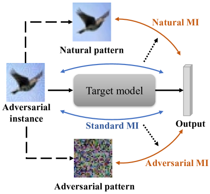
Figure 1: A visual illustration of disentangling the standard MI into the natural MI and the adversarial MI. The longdash lines show that the adversarial sample is disassembled into the natural pattern (derived from the natural sample) and the adversarial pattern (derived from the adversarial noise). The dotted lines denote the operation of disentangling the standard MI into the natural MI and the adversarial MI.

Based on the above MI estimation, we develop an adversarial defense algorithm called natural-adversarial mutual information-based defense (NAMID) to enhance the adversarial robustness. Specifically, we introduce an optimization strategy using the natural MI and the adversarial MI on the basis of the adversarial training manner. The optimization strategy is to maximize the natural MI of the input adversarial sample and minimize its adversarial MI simultaneously. By iteratively executing the procedures of generating adversarial samples and optimizing the model parameters, we can learn an adversarially robust target model.

The main contributions in this paper are as follows:

• Considering the adversarial sample has the natural pattern and the adversarial pattern, we propose the natural MI and the adversarial MI to explicitly measure the dependence of the output on the different patterns.

• We design a neural network-based method to effectively estimate the natural MI and the adversarial MI. By exploiting the MI estimation networks, we develop a defense algorithm to train a robust target model.

• We empirically demonstrate the effectiveness of the proposed defense algorithm on improving the classification accuracy. The evaluation experiments are conducted against multiple adversarial attacks.

The rest of this paper is organized as follows. In Section 2, we introduce some preliminary information and briefly review related works. In Section 3, we propose the natural MI and the adversarial MI, and develop an adversarial defense method. Experimental results are provided in Section 4. Finally, we conclude this paper in Section 5.

2 Preliminaries

In this section, we introduce some preliminary about notation, the problem setting and mutual information (MI). We also review some representative literature on adversarial attacks and defenses.

Notation. We use capital letters such as $X$ and $Y$ to represent random variables, and lower-case letters such as $x$ and $y$ to represent realizations of random variables $X$ and $Y$, respectively. For norms, we denote by $\|x\|$ a generic norm, by $\|x\|_{\infty}$ the $L_{\infty}$ norm of $x$, and by $\|x\|_{2}$ the $L_{2}$ norm of $x$. In addition, let $\mathbb{B}(x,\epsilon)$ represent the neighborhood of $x$: $\{\tilde{x}:\|\tilde{x}-x\|\leq\epsilon$}, where $\epsilon$ is the perturbation budget. We define the classification function as $f:\mathcal{X}\rightarrow\{1,2,\ldots,C\}$. It can be parameterized, e.g., by a deep neural network $h_{\theta}$ with model parameter $\theta$.

Problem setting. In this paper, we focuses on a classification task under the adversarial environment. Let $X$ and $Y$ be the variables for natural instances and ground-truth labels respectively. We sample natural data $\{(x_{i},y_{i})\}_{i=1}^{n}$ according to the distribution of variables $(X,Y)$. Given a pair of natural data $(x,y)$, the adversarial instance $\tilde{x}$ satisfies the following constraint:

$$f\left(\tilde{x}\right)\neq y\quad\text{ s.t.}\quad\left\|x-\tilde{x}\right\|\leq\epsilon\text{,}$$ (1)

where $\tilde{x}=x+n$, $n$ denotes the adversarial noise. Our aim is to develop an adversarial defense method to help train the classification model $h_{\theta}$ to make normal predictions.

Mutual information. MI is an entropy-based measure that can reflect the dependence degree between variables. A larger MI typically indicates a stronger dependence between the two variables. Various methods have been proposed for estimating MI (Moon et al., 1995; Darbellay & Vajda, 1999; Kandasamy et al., 2015; Moon et al., 2017). A representative and efficient estimator is the mutual information neural estimator (MINE) (Belghazi et al., 2018). MINE is empirically demonstrated its superiority in estimation accuracy and efficiency, and proved that it is strongly consistent with the true MI. Besides, the work in Hjelm et al. (2018) points that using the complete input to estimate MI is often insufficient for classification task. Instead, estimating MI between the high-level feature and local patches of the input is more suitable. Therefore, in this paper, we refer the local DIM estimator (Hjelm et al., 2018) to estimate MI. The definition of MI and other details are presented in Appendix A

Adversarial attacks. Adversarial noise can be crafted by optimization-based attacks, such as PGD (Madry et al., 2018), AA (Croce & Hein, 2020), CW (Carlini & Wagner, 2017) and DDN (Rony et al., 2019). Besides, some attacks such as FWA (Wu et al., 2020b) and STA (Xiao et al., 2018) focus on mimicking non-suspicious vandalism by exploiting the geometry and spatial information. These attacks constrain the perturbation boundary by a small norm-ball $\|\cdot\|_{p}\leq\epsilon$, so that their adversarial instances can be perceptually similar to natural instances.

Adversarial defenses. The issue of adversarial attacks promotes the development of adversarial defenses. A major class of adversarial defense methods is devoted to enhance the adversarial robustness in an adversarial training manner (Madry et al., 2018; Ding et al., 2019; Zhang et al., 2019; Wang et al., 2019). They augment training data with adversarial samples and use a min-max formulation to train the target model (Madry et al., 2018). However, these methods do not explicitly measure the dependence between the adversarial sample and its corresponding output. In addition, some data pre-processing based methods try to remove adversarial noise by learning denoising functions (Liao et al., 2018; Naseer et al., 2020; Zhou et al., 2021c) or feature-squeezing functions (Guo et al., 2018). However, these methods may suffer from the problems of human-observable loss (Xu et al., 2017) and residual adversarial noise (Liao et al., 2018), which would affect the final prediction. To avoid the above problems, we propose to exploit the natural MI and the adversarial MI to learn an adversarially robust classification model in the adversarial training manner.

3 Methodology

In this section, we first illustrate the motivation for using mutual information (MI) and disentangling the standard mutual information into the natural MI and the adversarial MI (Section 3.1). Next, we theoretically prove the reasonability of the disentanglement and introduce how to effectively estimate the natural MI and the adversarial MI (Section 3.2). Finally, we propose an adversarial defense algorithm which contains an MI-based optimization strategy (Section 3.3). The code is available at https://github.com/dwDavidxd/MIAT.

3.1 Motivation

For adversarial samples, The predictions of the target model are typically significantly irrelevant to the given objectives in the inputs. Studying the dependence between the adversarial sample and its corresponding output is considered to be beneficial for improving the adversarial robustness. The dependence could be exploited as supervision information to help train the target model to make correct predictions.

Estimating the standard MI of the adversarial sample (i.e., the MI between the adversarial sample and its corresponding output in a target model) is a simple strategy to measure the dependence. However, different from natural samples, adversarial samples have two patterns, i.e., the natural pattern and the adversarial pattern. The standard MI cannot respectively consider the dependence of the output on the different patterns, which may limit its performance in helping the target model improve the adversarial robustness.

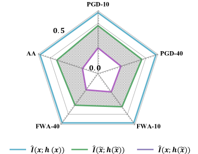
Figure 2: The visualization of the proof-of-concept experiment. Given the natural instance $x$, its adversarial instance $\tilde{x}$ and a target model $h$, the logit output of $h$ for $\tilde{x}$ is denoted by $h(\tilde{x})$. We respectively estimate the standard MI of the natural instance $\widehat{I}(x,h(x))$, the standard MI of the adversarial instance $\widehat{I}(\tilde{x},h(\tilde{x}))$ and the MI between $h(\tilde{x})$ and $x$. The shaded area represents the difference between $\widehat{I}(\tilde{x},h(\tilde{x}))$ and $\widehat{I}(x,h(\tilde{x}))$.

Specifically, the natural pattern is derived from the original natural sample. It provides available information for the target model to produce the right output. The adversarial pattern is derived from the adversarial noise. It controls the flip of the prediction from the correct label to the wrong label (Ilyas et al., 2019). Both the natural and adversarial patterns cause important impacts on the output, but they are mutually exclusive. Therefore, the standard MI actually measures a confused dependence.

To clearly illustrate the confused dependence, we conduct a proof-of-concept experiment. We randomly select a set of natural instances and use five attacks to generative adversarial instances. We use a classification model as the target model. The MI estimator is trained on natural instances and their outputs via the MI maximization (Hjelm et al., 2018). By exploiting the estimator, we respectively estimate the standard MI of the natural instance, the standard MI of the adversarial instance and the MI between the natural instance and the output for the corresponding adversarial instance. The details of the experiment are presented in Appendix B

As shown in Figure 2, the result shows that the standard MI of the adversarial sample is indeed smaller than that of the natural sample. However, it is still significantly larger than the MI between the output and natural pattern only (see the pink line). This shows that the standard MI of the adversarial sample contains the dependence of the output on the adversarial pattern. Thus, maximizing the standard MI may increase the dependence of the output on the adversarial pattern and cause more disturbance to the prediction. Directly maximizing the standard MI cannot comprehensively promote the target model to make more accurate predictions for adversarial samples.

To solve this problem, in this paper, we propose to disentangle the standard MI into two parts related to the natural and adversarial patterns respectively.

3.2 Natural MI and adversarial MI

We define two new concepts: natural mutual information (natural MI) and adversarial mutual information (adversarial MI). The natural MI is MI between the output and the natural pattern of the input. The adversarial MI is MI between the output and the adversarial pattern of the input. To explicitly measure the dependence of the output on different patterns of the input, we need to disentangle the standard MI into the natural MI and the adversarial MI.

3.2.1 Disentangling the standard MI

In this section, we introduce how to disentangle the standard MI and describe the reasonability of the disentanglement. We first provide Theorem 1 to illustrate the transformation relationship of MI among four variables.

Theorem 1. Let $X,\widetilde{X},N,Z$ denote four random variables respectively, where $\widetilde{X}=X+N$. Let $\widetilde{\mathcal{X}}$ be the feature space of $\widetilde{X}$ and $\mathcal{Z}$ be the feature space of $Z$. Then, for any function $h:\widetilde{\mathcal{X}}\rightarrow\mathcal{Z}$, we have

$$I(\widetilde{X};Z) =I(X;Z)+I(N;Z)-I(X;N;Z)$$ (2)

$$+H(Z|X,N)-H(Z|\widetilde{X})\text{,}$$

where $I(\cdot;\cdot)$ denotes the MI between two variables and $I(\cdot;\cdot;\cdot)$ denotes the MI between two three variables. A detailed proof is provided in Appendix C.

Then, we apply Theorem 1 to the adversarial learning setting and obtain Corollary 1.

Corollary 1. Let $X,\widetilde{X},N$ denote the random variables for the natural instance, adversarial instance and adversarial noise respectively, where $\widetilde{X}=X+N$. Given a function parameterized by a target model $h_{\theta}$ with model parameter $\theta$, the logit output of $h_{\theta}$ for $\widetilde{X}$ is denoted by $h_{\theta}(\widetilde{X})$. Considering that the effects of the natural instance and the adversarial noise on the output are mutually exclusive, we assume that the MI between $X,N$ and $h_{\theta}(\widetilde{X})$ (i.e., $I(X;N;h_{\theta}(\widetilde{X}))$) is small. We also assume that the difference between $H(Z|X,N)$ and $H(Z|\widetilde{X})$ is small (see Appendix D for more details), then we have:

$$I(\widetilde{X};h_{\theta}(\widetilde{X}))\approx\underbrace{I(X;h_{\theta}(\widetilde{X}))}_{I_{N}}+\underbrace{I(N;h_{\theta}(\widetilde{X}))}_{I_{A}}\text{,}$$ (3)

where $I_{N}$ denote the MI between the output and the natural instance and $I_{A}$ denote the MI between the output and the adversarial noise.

Actually, we could use the original natural instance and the adversarial noise to represent the natural pattern and the adversarial pattern of the input respectively. In this way, $I_{N}$ and $I_{A}$ could denote the natural MI and the adversarial MI respectively.

According to Equation 3, we can approximately disentangle the standard MI into the natural MI and the adversarial MI. The latter two can not only reflect the dependency between input and output as the former, but also provides independent measurements for different patterns. This is more conducive to designing specific optimization strategies for the two patterns to better alleviate the negative effects of the adversarial noise.

3.2.2 Estimating the natural MI and the adversarial MI

The local DIM estimation method has been demonstrated to be efficient for estimating MI (Hjelm et al., 2018; Zhu et al., 2020). We thus first use this method to train a estimation network for the natural MI and the adversarial MI respectively. Let $E_{\phi_{n}}$ denote the estimation network for the natural MI and $E_{\phi_{a}}$ denote the estimation network for the adversarial MI. Considering the inherent close relevance between the natural/adversarial pattern and the output for the natural/adversarial sample, we naturally use the natural/adversarial samples to train the $E_{\phi_{n}}$/$E_{\phi_{a}}$. The optimization goals for $\phi_{n}$ and $\phi_{a}$ are as follows:

$$\widehat{\phi}_{n}=\underset{\phi_{n}\in\Phi_{N}}{\arg\max}\,E_{\phi_{n}}(h_{\theta_{0}}(X))\text{,}$$ (4)

$$\widehat{\phi}_{a}=\underset{\phi_{a}\in\Phi_{A}}{\arg\max}\,E_{\phi_{a}}(h_{\theta_{0}}(\widetilde{X}))\text{,}$$

where $\Phi_{N}$ and $\Phi_{A}$ denote the sets of model parameters, $h_{\theta_{0}}$ denotes the pre-trained target model. It can be naturally trained or be adversarially trained. We use a ResNet-18 optimized by standard AT (Madry et al., 2018) as the pre-trained model $h_{\theta_{0}}$. $E_{\widehat{\phi}_{n}}\left(\cdot\right)$ is the estimated natural MI and $E_{\widehat{\phi}_{a}}\left(\cdot\right)$ is the estimated adversarial MI, i.e., $E_{\widehat{\phi}_{n}}\left(h_{\theta}(X)\right)=\widehat{I}_{N}(X;h_{\theta}(X))$, $E_{\widehat{\phi}_{n}}(h_{\theta}(\widetilde{X}))=\widehat{I}_{N}(X;h_{\theta}(\widetilde{X}))$ and $E_{\widehat{\phi}_{a}}\left(h_{\theta}(X)\right)=\widehat{I}_{A}(N;h_{\theta}(X))$, $E_{\widehat{\phi}_{a}}(h_{\theta}(\widetilde{X}))=\widehat{I}_{A}(N;h_{\theta}(\widetilde{X}))$.

By exploiting the two MI estimation network, we estimate the natural MI of the natural sample and the adversarial sample (i.e., $\widehat{I}_{N}(X,h_{\theta_{0}})$ and $\widehat{I}_{N}(\widetilde{X},h_{\theta_{0}})$), and the adversarial MI of the natural sample and the adversarial sample (i.e., $\widehat{I}_{A}(X,h_{\theta_{0}})$ and $\widehat{I}_{N}(\widetilde{X},h_{\theta_{0}})$), respectively. We find that adversarial samples usually have larger adversarial MI and smaller natural MI compared with those w.r.t. natural samples, which is consistent with our intuitive cognition. However, the change is relatively insignificant, and thus has limitations in reflecting the difference between the adversarial sample and the natural sample in the natural MI and the adversarial MI. We will show this observation later in Section 4.2.

To adequately represent the inherent difference in the natural MI and the adversarial MI between the natural sample and the adversarial sample, we design an optimization mechanism for the MI estimation. This is, we minimize the natural MI of the adversarial sample and minimize the adversarial MI of the natural sample during training the estimators. In addition, to estimate the two MI more accurately, we select samples that are correctly predicted by the target model and the corresponding adversarial samples are wrongly predicted, to train the estimation networks. The reformulated optimization goals are as follows:

$$\widehat{\phi}_{n}=\underset{\phi_{n}\in\Phi_{N}}{\arg\max}\,[E_{\phi_{n}}(h_{\theta_{0}}(X^{\prime}))-E_{\phi_{n}}(h_{\theta_{0}}(\widetilde{X}^{\prime}))]\text{,}$$ (5)

$$\widehat{\phi}_{a}=\underset{\phi_{a}\in\Phi_{A}}{\arg\max}\,[E_{\phi_{a}}(h_{\theta_{0}}(\widetilde{X}^{\prime}))-E_{\phi_{a}}\left(h_{\theta_{0}}(X^{\prime}\right))]\text{,}$$

where $X^{\prime}$ is the selected data:

$$X^{\prime}=\arg_{X}\left[\delta\left(h_{{\theta}_{0}}(X)\right)=Y\&\delta(h_{{\theta}_{0}}(\widetilde{X}))\neq Y\right]\text{,}$$ (6)

where $\delta$ is the operation that transforms the logit output into the prediction label.

3.3 Adversarial defense algorithm

Based on the above two MI estimation networks, we develop an adversarial defense algorithm called natural-adversarial mutual information-based defense (NAMID) to enhance the adversarial robustness. In this section, we first introduce the natural-adversarial MI-based optimization strategy and then illustrate the training algorithm.

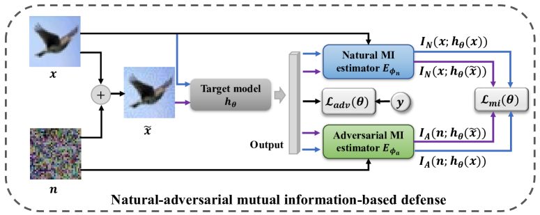
Figure 3: The overview of our proposed NAMID adversarial defense algorithm.

3.3.1 natural-adversarial MI-based defense

According to the observations and analysis in Section 3.1 and Section 3.2, we plan to use the natural MI and the adversarial MI to help train the target model. We aim to guide the target model to increase the attention to the natural pattern while reducing the attention to the adversarial pattern.

Specifically, The optimization strategy is to maximize the natural MI of the input adversarial sample and minimize its adversarial MI simultaneously. The optimization goal for the target model is as follows:

$$\widehat{\theta}=\underset{\theta\in\Theta}{\arg\max}\left[E_{\widehat{\phi}_{n}}(h_{\theta}(\widetilde{X}))-E_{\widehat{\phi}_{a}}(h_{\theta}(\widetilde{X}))\right]\text{.}$$ (7)

To achieve the optimization goal, we can directly utilize the natural and adversarial MI of the adversarial sample to construct a loss function. However, this loss function does not consider the difference in natural/adversarial MI between the natural sample and the adversarial sample. Thus, we transform this absolute metric-based loss to a relative metric-based loss. In addition, as described in Section 3.2.2, we use the selected samples to compute the loss function. The loss function is formulated as:

$$\begin{gathered}\mathcal{L}_{mi}(\theta)=\frac{1}{m}\sum_{i=1}^{m}\{\mathcal{L}_{\cos}(E_{\widehat{\phi}_{n}}(h_{\theta}(\tilde{x}_{i}^{\prime})),E_{\widehat{\phi}_{n}}(h_{\theta}(x_{i}^{\prime})))\\ +\mathcal{L}_{\cos}(E_{\widehat{\phi}_{a}}(h_{\theta}(\tilde{x}_{i}^{\prime}),E_{\widehat{\phi}_{a}}(h_{\theta}(x_{i}^{\prime})))\\ +\lambda\cdot[E_{\widehat{\phi}_{a}}(h_{\theta}(\tilde{x}_{i}^{\prime}))-E_{\widehat{\phi}_{n}}(h_{\theta}(\tilde{x}_{i}^{\prime}))]\}\text{,}\end{gathered}$$ (8)

where $m$ is the number of the selected data $X^{\prime}$ and $\lambda$ is a hyperparameter. $\mathcal{L}_{\cos}(\cdot,\cdot)$ is the cosine similarity-based loss function, i.e., $\mathcal{L}_{\cos}(a,b)=||1-sim(a,b)||_{1}$, $sim(\cdot,\cdot)$ denotes the cosine similarity measure.

The MI-based optimization strategy can exploited together with the adversarial training manner. The overall loss function for training the target model is as follows:

$$\mathcal{L}_{all}(\theta)=\mathcal{L}_{adv}(\theta)+\alpha\cdot\mathcal{L}_{mi}(\theta)\text{,}$$ (9)

where $\mathcal{L}_{adv}(\theta)$ is the loss function of the adversarial training method, which is typically the cross-entropy loss between the adversarial outputs and the ground-truth labels: $\mathcal{L}_{adv}(\theta)=-\frac{1}{n}\sum_{i=1}^{n}[\boldsymbol{y_{i}}\cdot\log(\sigma(h_{\theta}(\tilde{x}_{i})))]$. $n$ is the number of training samples and $\sigma$ denotes the softmax function. $\alpha$ is a trade-off hyperparameter. We provide the overview of the adversarial defense method in Figure 3.

3.3.2 Training algorithm

We conduct the adversarial training on the procedures of generating adversarial samples and optimizing the target model parameter. The details of the overall procedure are presented in Algorithm 1.

Specifically, the procedure requires the target model $h_{\theta}$ with parameter $\theta$, the natural MI estimation network with parameter $\widehat{\phi}_{n}$, the adversarial MI estimation network with parameter $\widehat{\phi}_{a}$ and perturbation budget $\epsilon$. For the natural instance $x$ in mini-batch $\mathcal{B}=\{x_{i}\}_{i=1}^{n}$ sampled from natural training set, we first craft adversarial noise $n$ and generate adversarial instance $\tilde{x}$ via the powerful PGD adversarial attack (Madry et al., 2018). Then, we input the natural and adversarial training data into the target model $h_{\theta}$ and obtain the selected instance $x^{\prime}$, $\tilde{x}^{\prime}$ according to Equation 6. Next, we estimate the natural MI $E_{\widehat{\phi}_{n}}(h_{\theta}(x^{\prime})),E_{\widehat{\phi}_{n}}(h_{\theta}(\tilde{x}^{\prime}))$ and the adversarial MI $E_{\widehat{\phi}_{a}}(h_{\theta}(x^{\prime})),E_{\widehat{\phi}_{a}}(h_{\theta}(\tilde{x}^{\prime})$. Finally, we optimize the parameter $\theta$ according to Equation 9. By iteratively conduct the adversarial training, $\theta$ is expected to be optimized well.

Algorithm 1 Natural-adversarial mutual information-based defense (NAMID) algorithm

0:  Target model $h_{\theta}(\cdot)$ parameterized by $\theta$, natural MI estimation network $E_{\widehat{\phi}_{n}}$, adversarial MI estimation network $E_{\widehat{\phi}_{a}}$, batch size $n$, and the perturbation budget $\epsilon$;

1:  repeat

2:     Read mini-batch $\mathcal{B}=\{x_{i}\}_{i=1}^{n}$ from training set;

3:     for $i=1$ to $n$ (in parallel) do

4:       Craft adversarial noise $n_{i}$ and generate adversarial instance $\tilde{x}_{i}$ at the given perturbation budget $\epsilon$ for $x_{i}$;

5:       Forward-pass $x_{i}$, $\tilde{x}_{i}$ through $h_{\theta}(\cdot)$ and obtain $h_{\theta}(x_{i})$, $h_{\theta}(\tilde{x}_{i})$;

6:       Select samples according to Equation 6;

7:     end for

8:     Calculate $\mathcal{L}_{all}$ using Equation 9 and optimize $\theta$;

9:  until training converged.

4 Experiments

In this section, we first introduce the experiment setups including datasets, attack setting and defense setting in Section 4.1. Then, we show the effectiveness of our optimization mechanism for evaluating MI in Section 4.2. Next, we evaluate the performances of the proposed adversarial defense algorithm in Section 4.3. Finally, we conduct ablation studies in Section 4.4.

4.1 Experiment setups

Datasets. We verify the effective of our defense algorithm on two popular benchmark datasets, i.e., CIFAR-10 (Krizhevsky et al., 2009) and Tiny-ImageNet (Wu et al., 2017). CIFAR-10 has 10 classes of images including 50,000 training images and 10,000 test images. Tiny-ImageNet has 200 classes of images including 100,000 training images, 10,000 validation images and 10,000 test images. Images in the two datasets are all regarded as natural instances. All images are normalized into [0,1], and are performed simple data augmentations in the training process, including random crop and random horizontal flip.

Model architectures. We use a ResNet-18 (He et al., 2016) as the target model for both CIFAR-10 and Tiny-ImageNet. For the MI estimation network, we utilize the same neural network as in (Zhu et al., 2020). The estimation networks for the natural MI and the adversarial MI have same model architectures.

Baselines. (1) Standard AT (Madry et al., 2018); (2) TRADES (Zhang et al., 2019); (3) MART (Wang et al., 2019); and (4)WMIM: A defense that refers to Zhu et al. (2020). The first three are representative adversarial training methods, and the last one combines adversarial training with standard MI maximization (on adversarial samples).

Attack settings. Adversarial data for evaluating defense models are crafted by applying state-of-the-art attacks. These attacks are divided into two categories: $L_{\infty}$-norm attacks and $L_{2}$-norm attacks. The $L_{\infty}$-norm attacks include PGD (Madry et al., 2018), AA (Croce & Hein, 2020), TI-DIM (Dong et al., 2019; Xie et al., 2019), and FWA (Wu et al., 2020b). The $L_{2}$-norm attacks include PGD, CW₂ (Carlini & Wagner, 2017) and DDN (Rony et al., 2019). Among them, the AA attack algorithm integrates three non-target attacks and a target attack. Other attack algorithms are utilized as non-target attacks. The iteration number of PGD and FWA is set to 40 with step size $\epsilon/4$. The iteration number of CW₂ and DDN are set to 20 respectively with step size 0.01. For CIFAR-10 and Tiny-ImageNet, the perturbation budgets for $L_{2}$-norm attacks and $L_{\infty}$-norm attacks are $\epsilon=0.5$ and $8/255$ respectively.

Defense settings. For both CIFAR-10 and Tiny-ImageNet, the adversarial training data for $L_{\infty}$-norm and $L_{2}$-norm is generated by using $L_{\infty}$-norm PGD-10 and $L_{2}$-norm PGD-10 respectively. The step size is $\epsilon/4$ and the perturbation budget is $8/255$ and $0.5$ respectively. The epoch number is set to 100. For fair comparisons, all the methods are trained using SGD with momentum 0.9, weight decay $2\times 10^{-4}$, batch-size 1024 and an initial learning rate of 0.1, which is divided by 10 at the 75-th and 90-th epoch. In addition, we adjust the hyperparameter settings of the defense methods so that the natural accuracy is not severely compromised and then compare the adversarial accuracy. We set $\alpha=5,\lambda=0.1$ for our algorithm.

4.2 Effectiveness of MI estimation networks

In Section 3.2.2, we point out that training the MI estimation network directly by MI maximization may not clearly reflect the difference between the adversarial sample and the natural sample in natural MI and adversarial MI. We thus design an optimization mechanism for training the MI estimation network. To demonstrate the effectiveness of the optimization mechanism, we compare the performance of the estimation networks trained by Equation 4 and Equation 5 in Figure 4. The performances of the defenses based on the two different estimators are shown in Section E.1

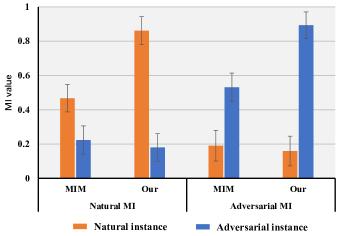
Figure 4: The performances of MI estimation networks trained by Equation 4 (MIM) and Equation 5 (Our). The left half is the estimated natural MI, and the right half is the adversarial MI.

Table 1: Adversarial accuracy (percentage) of defense methods against white-box attacks on CIFAR-10 and Tiny-ImageNet. The target model is ResNet-18.

Dataset	Defense	$L_{\infty}$-norm					$L_{2}$-norm
		None	PGD-40	AA	FWA-40	TI-DIM	None	PGD-40	CW	DDN
CIFAR-10	Standard	83.39	42.38	39.01	15.44	55.63	83.97	61.69	30.96	29.34
	WMIM	80.32	40.76	36.05	12.14	53.10	81.29	58.36	28.41	27.13
	NAMID	83.41	44.79	39.26	15.67	58.23	84.35	62.38	34.48	32.41
2-11[3pt/5pt]	TRADES	80.70	46.29	42.71	20.54	57.06	83.72	63.17	33.81	32.06
	NAMID_T	80.67	47.53	43.39	21.17	59.13	84.19	64.75	35.41	34.27
2-11[3pt/5pt]	MART	78.21	50.23	43.96	25.56	58.62	83.36	65.38	35.57	34.69
	NAMID_M	78.38	51.69	44.42	25.64	61.26	84.07	66.03	36.19	35.76
Tiny-ImageNet	Standard	48.40	17.35	11.27	10.29	27.84	49.57	26.19	12.73	11.25
	WMIM	47.43	16.50	9.87	9.25	25.19	48.16	24.10	11.35	10.16
	NAMID	48.41	18.67	12.29	11.32	29.37	49.65	28.13	14.29	12.57
2-11[3pt/5pt]	TRADES	48.25	19.17	12.36	10.67	29.64	48.83	27.16	13.28	12.34
	NAMID_T	48.21	20.12	12.86	14.91	30.81	49.07	28.83	14.47	13.91
2-11[3pt/5pt]	MART	47.83	20.90	15.57	12.95	30.71	48.56	27.98	14.36	13.79
	NAMID_M	47.80	21.23	15.83	15.09	31.59	48.72	29.14	15.06	14.23

We use the test data from CIFAR-10 to evaluate the performance. For the natural MI, we offset the estimated MI so that the worst-case of the natural MI equals 0, and calculate the average of all samples. Similarly, we offset the estimated MI so that the worst-case of the adversarial MI equals 0. Note that for a fair comparison, we use selected samples to train the estimation networks for both methods. As shown in Figure 4, the results demonstrate that the optimization mechanism could help adequately represent the inherent difference in the natural MI and the adversarial MI between the natural sample and the adversarial sample.

4.3 Robustness evaluation and analysis

To demonstrate the effectiveness of our adversarial defense algorithm, we evaluate the adversarial accuracy using white-box and black-box adversarial attacks, respectively.

White-box attacks. In the white-box setting, all attacks can access the architectures and parameters of target models. We evaluate the robustness by exploiting six types of adversarial attacks for both CIFAR-10 and Tiny-ImageNet: $L_{\infty}$-norm PGD, FWA, AA, TI-DIM attacks and $L_{2}$-norm PGD, DDN, CW attacks. The average natural accuracy (i.e., the results in the third column) and the average adversarial accuracy of defenses are shown in Table 1.

The results show that our method (i.e., NAMID) can achieve better robustness compared with Standard AT. The performance of our method on the natural accuracy is competitive (83.39% vs. 83.41%), and it provides more gains on adversarial accuracy (e.g., 5.69% against PGD-40). Compared with WMIM, the results show that our proposed strategy of disentangling the standard MI into the natural MI and the adversarial MI is effective. The standard deviation is shown in Section E.2.

Note that the default adversarial training loss in our method (i.e., $\mathcal{L}_{adv}$ in Equation 9) is the same as Standard AT. To avoid the bias caused by different adversarial training methods, we apply the adversarial training losses of TRADES and MART to our method respectively (i.e., NAMID_T and NAMID_M). As shown in Table 1, the results show that our method can improve the adversarial accuracy (e.g., the accuracy against PGD is improved by 2.68% and 2.91% compared with TRADES and MART on CIFAR-10).

Black-box attacks. Block-box adversarial instances are crafted by attacking a surrogate model. We use a VggNet-19 (He et al., 2016) as the surrogate model. The surrogate models and the defense models are trained separately. We use Standard AT method to train the surrogate model and use PGD, AA and FWA to generate adversarial test data. The performances of our defense method is reported in Table 2. The results show that our method is a practical strategy for real scenarios, which can protect the target model from black-box attacks by malicious adversaries.

Table 2: Adversarial accuracy (percentage) of defense methods against black-box attacks on CIFAR-10. The target model is ResNet-18 and the surrogate model is adversarially trained VggNet-19. We show the most successful defense with bold.

Defense	None	PGD-40	AA	FWA-40
Standard	83.39	65.88	60.93	56.42
WMIM	80.32	62.79	57.86	53.05
NAMID	83.41	69.57	63.72	59.30

4.4 Ablation study

To clearly elucidate the role of each component of our method in improving adversarial robustness, we conduct ablation studies in three different settings: (i) removing the adversarial MI; (ii) removing the natural MI; and (iii) setting the hyperparameter $\lambda$ (in Equation 8) to 0. We use $L_{\infty}$-norm PGD and FWA attacks to evaluate the performances of these variants. As shown in Figure 5, the results demonstrate that each component of our method contributes positively to improving adversarial accuracy.

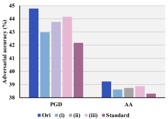
Figure 5: The ablation study.The bars with different colors represent the performance under different settings. Among them, ’Ori’ denotes our method NAMID and ’Standard’ denotes Standard AT.

5 Conclusion

To the best of our knowledge, the dependence between the output of the target model and input adversarial samples have not been well studied. In this paper, we investigate the dependence from the perspective of information theory. Considering that adversarial samples contain natural and adversarial patterns, we propose to disentangle the standard MI into the natural MI and the adversarial MI to explicitly measure the dependence of the output on the different patterns. We design a neural network-based method to train two MI estimation networks to estimate the natural MI and the adversarial MI. Based on the above MI estimation, we develop an adversarial defense algorithm called natural-adversarial mutual information-based defense (NAMID) to enhance the adversarial robustness. The empirical results demonstrate that our defense method can provide effective protection against multiple adversarial attacks. Our work provides a new adversarial defense strategy for the community of adversarial learning. In future, we will design more efficient mechanisms for training MI estimators and further optimize the natural-adversarial MI-based defense to improve the performance against stronger attacks. In addition,

6 Acknowledgements

This work was supported in part by the National Key Research and Development Program of China under Grant 2018AAA0103202, in part by the National Natural Science Foundation of China under Grant 61922066, 61876142, 62036007, 62006202, 61922066, 61876142, 62036007, and 62002090, in part by the Technology Innovation Leading Program of Shaanxi under Grant 2022QFY01-15, in part by Open Research Projects of Zhejiang Lab under Grant 2021KG0AB01, in part by the RGC Early Career Scheme No. 22200720, in part by Guangdong Basic and Applied Basic Research Foundation No. 2022A1515011652, in part by Australian Research Council Projects DE-190101473, IC-190100031, and DP-220102121, in part by the Fundamental Research Funds for the Central Universities, and in part by the Innovation Fund of Xidian University. The authors thank the reviewers and the meta-reviewer for their helpful and constructive comments on this work.

Appendix A Related work on mutual information

Mutual information (MI) is an entropy-based measure that can reflect the dependence degree between variables. The definition of MI is as follows.

Definition 1. Let $(X,Z)$ be a pair of random variables and $\mathcal{X}\times\mathcal{Z}$ be their feature space. The MI of $(X,Z)$ is defined as:

$$I(X;Z)=\int_{Z}\int_{\mathcal{X}}p_{XZ}(x,z)\log\left(\frac{p_{XZ}(x,z)}{p_{X}(x)p_{Z}(z)}\right)dxdz\text{,}$$ (10)

where $p_{XZ}$ is the joint probability density function of $(X,Z)$, and $p_{X}$, $p_{Z}$ are the marginal probability density functions of $X$ and $Z$ respectively.

Intuitively, $I(X;Z)$ could reflect how well one can predict $Z$ from $X$ (and $X$ from $Z$, since it is symmetrical (Zhu et al., 2020)). By definition, $I(X;Z)=0$ if $X$ and $Z$ are independent; A larger MI typically indicates a stronger dependence between the two variables.

Various methods have been proposed for estimating MI (Moon et al., 1995; Darbellay & Vajda, 1999; Kandasamy et al., 2015; Moon et al., 2017). A representative and efficient estimator is the mutual information neural estimator (MINE) (Belghazi et al., 2018):

$$\widehat{I}_{\omega}(X;Z)=\sup_{\omega\in\Omega}\mathbb{E}_{\widehat{\mu}_{XZ}^{(n)}}\left[T_{\omega}\right]-\log\left(\mathbb{E}_{\widehat{\mu}_{X}^{(n)}\otimes\widehat{\mu}_{Z}^{(n)}}\left[\exp\left(T_{\omega}\right)\right]\right)\text{,}$$ (11)

where $T_{\omega}:\mathcal{X}\times\mathcal{Z}\rightarrow\mathbb{R}$ is a function modeled by a neural network with parameters $\omega\in\Omega$. $\widehat{\mu}_{XZ}^{(n)}$ , $\mu_{X}^{(n)}$ and $\mu_{Z}^{(n)}$ are the empirical distributions of random variables $(X,Z)$, $X$ and $Z$ respectively, associated to n $i.i.d.$ samples. MINE is empirically demonstrated its superiority in estimation accuracy and efficiency, and proved that it is strongly consistent with the true MI.

Besides, the work in Hjelm et al. (2018) points that using the complete input to estimate MI is often insufficient for classification task. Instead, estimating MI between the high-level feature and local patches of the input is more suitable. This work propose a local DIM estimator to estimate MI:

$$\widehat{I}_{\psi,\omega}(X;Z)=\widehat{I}_{\omega}(C_{\psi}(X);Z)\text{,}$$ (12)

where $C_{\psi}$ is a encoder modeled by a neural network with parameter $\psi$. It encode the input to a local feature map that reflects useful structure in the data (e.g., spatial locality). In this paper, we refer the local DIM estimator to estimate the natural MI and the adversarial MI.

Appendix B Proof-of-concept experiment

We randomly select 1,000 natural test samples from CIFAR-10 as the experimental data. We exploit three representative adversarial attacks (i.e., PGD (Madry et al., 2018), AA (Croce & Hein, 2020) and FWA (Wu et al., 2020b)) with different iteration numbers to generative adversarial samples respectively. We use a naturally trained ResNet-18 network (He et al., 2016) as the target model $h$. We respectively estimate the standard MI of the natural sample $\widehat{I}(x,h(x))$, the standard MI of the adversarial sample $\widehat{I}(\tilde{x},h(\tilde{x}))$ and the MI between the natural sample and the output for the corresponding adversarial sample $\widehat{I}(x,h(\tilde{x}))$ via the local DIM estimator. Note that the natural MI of the natural sample is equivalent to its standard MI. We offset the estimated MI so that the worst-case of the estimated MI equals 0, and then calculate the average of all samples for $\widehat{I}(x,h(x))$, $\widehat{I}(\tilde{x},h(\tilde{x}))$ and $\widehat{I}(x,h(\tilde{x}))$ respectively.

Appendix C Proof of Theorem 1

In this section, we provide the proof of the theoretical result in Section 3.2.1.

Theorem 1. Let $X,\widetilde{X},N,Z$ denote four random variables respectively, where $\widetilde{X}=X+N$. Let $\widetilde{\mathcal{X}}$ be the feature space of $\widetilde{X}$ and $\mathcal{Z}$ be the feature space of $Z$. Then, for any function $h:\widetilde{\mathcal{X}}\rightarrow\mathcal{Z}$, we have

$$I(\widetilde{X};Z)=I(X;Z)+I(N;Z)-I(X;N;Z)+H(Z|X,N)-H(Z|\widetilde{X})\text{,}$$ (13)

where $I(\cdot;\cdot)$ denotes the mutual information between two variables and $I(\cdot;\cdot;\cdot)$ denotes the mutual information between three variables.

Proof. According to the relationship between information entropy and mutual information, we first provide the following Lemma 1:

$$\left\{\begin{array}[]{l}I(\widetilde{X};Z)=H(Z)-H(Z|\widetilde{X})\\ I(X;Z)=H(Z)-H(Z|X)\\ I(N;Z)=H(Z)-H(Z|N)\end{array}\right.\text{,}$$ (14)

where $H(\cdot)$ denotes the information entropy, and $H(\cdot|\cdot)$ denotes the conditional information entropy.

According to Lemma 1, we have:

$$I(X;Z)+I(N;Z) =H(Z)-H(Z|X)+H(Z)-H(Z|N)$$ (15)

$$=2\,H(Z)-[H(Z|X)+H(Z|N)]\text{.}$$

According to the theorem of conditional mutual information in probability theory, we have:

$$H(Z|X)+H(Z|N) =[H(Z|X,N)+I(Z;N|X)]+[H(Z|X,N)+I(X;Z|N)]$$ (16)

$$=2\,H(Z|X,N)+I(Z;N|X)+I(X;Z|N)$$

$$=[H(Z|X,N)+I(Z;N|X)+I(X;Z|N)+I(X;N;Z)]$$

$$\;\;\;\;\;+H(Z|X,N)-I(X;N;Z)$$

$$=H(Z)+H(Z|X,N)-I(X;N;Z)\text{.}$$

Combining Equation 15 and Equation 16, we have:

$$I(X;Z)+I(N;Z) =2\,H(Z)-[H(Z)+H(Z|X,N)-I(X;N;Z)]$$ (17)

$$=H(Z)-H(Z|X,N)+I(X;N;Z)$$

$$=I(\widetilde{X};Z)+H(Z|\widetilde{X})-H(Z|X,N)+I(X;N;Z)\text{.}$$

Finally, we have:

$$I(\widetilde{X};Z)=I(X;Z)+I(N;Z)-I(X;N;Z)+H(Z|X,N)-H(Z|\widetilde{X})\text{,}$$ (18)

which completes the proof.

Appendix D The assumptions in Eq. (3).

The adversarial noise usually depends on the natural instance, that is, there is also a dependence between the adversarial noise and the natural sample. The MI between the natural sample and the adversarial noise (i.e., $I(X;N)$) may cause some effects on the disentanglement of standard MI in Equation 3. In fact, the effect of this MI is tiny. We illustrate this using two Venn diagrams.

As shown in Figure 6, since the adversarial noise is usually crafted based on the natural instance, $H(X)$ and $H(N)$ have a large overlap ($H$ denotes entropy). Considering that predictions are zero-sum (i.e., either right or wrong), and the effects of natural and adversarial patterns on outputs are mutually exclusive, $H(h(\widetilde{X}))$ either has a large overlap with $H(X)$ and a small overlap with $H(N)$ (Figure 6(a)), or has a large overlap with $H(N)$ and a small overlap with $H(X)$ (Figure 6(b)). In both cases, the overlap common to $H(X)$, $H(N)$, and $H(h(\widetilde{X}))$ (i.e., $I(X;N;h(\widetilde{X}))$) is small. Thus, $I(X;N)$ does not significantly affect Equation 3.

In addition, for the difference between $H(Z|X,N)$ and $H(Z|\widetilde{X})$, if we can recover the natural sample $X$ and the adversarial noise $N$ from $X+N$, then $X+N$ can contain all the information of $X$ and $N$, so the difference $H(Z|X,N)-H(Z|X+N)$ equals 0. Of course, this recovery process is difficult to precisely implement. Considering that we use $\widetilde{X}=X+N$ to generate adversarial sample in our work, we can precisely obtain $X$ and $N$, so we assume that the difference $H(Z|X,N)-H(Z|X+N)$ may tend to be small.

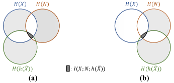
Figure 6: Venn diagrams for mutual information.

Appendix E Experimental results

E.1 Different MI estimation networks

We use the MI estimation network trained by Equation 4 and Equation 5 to train our adversarial defense model, respectively. The results are shown in Figure 7. From the results, it can be seen that our proposed method for training the MI estimation network can better facilitate the defense model to improve the adversarial accuracy.

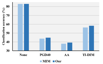
Figure 7: The performances of the defense based on different estimation networks. ’MIM’ denotes the defense model based on the MI estimation network trained by Equation 4. ’Our’ denotes the defense model based on the MI estimation network trained by Equation 5.

E.2 Defense against adversarial attacks

We show the performances of our defense algorithm against white-box $L_{\infty}$-norm attacks and $L_{2}$-norm attacks in Table 3 and Table 4, respectively. The performances of our defense algorithm against black-box $L_{\infty}$-norm attacks and $L_{2}$-norm attacks are shown in Table 5 and Table 6.

Table 3: Adversarial accuracy (percentage) of defense methods against $L_{\infty}$-norm white-box attacks on CIFAR-10 and Tiny-ImageNet. The target model is ResNet-18. The adversarial training data is crafted by using $L_{\infty}$-norm PGD-10.

Dataset	Defense	None	PGD-40	AA	FWA-40	TI-DIM
CIFAR-10	Standard	83.39$\pm$0.95	42.38$\pm$0.56	39.01$\pm$0.51	15.44$\pm$0.32	55.63$\pm$0.67
	WMIM	80.32$\pm$0.60	40.76$\pm$0.45	36.05$\pm$0.57	12.14$\pm$0.46	53.10$\pm$0.53
	NAMID	83.41$\pm$0.56	44.79$\pm$0.50	39.26$\pm$0.56	15.67$\pm$0.47	58.23$\pm$0.63
2-7[3pt/5pt]	TRADES	80.70$\pm$0.63	46.29$\pm$0.59	42.71$\pm$0.49	20.54$\pm$0.47	57.06$\pm$0.51
	NAMID_T	80.67$\pm$0.73	47.53$\pm$0.59	43.39$\pm$0.83	21.17$\pm$0.44	59.13$\pm$0.72
2-7[3pt/5pt]	MART	78.21$\pm$0.65	50.23$\pm$0.70	43.96$\pm$0.67	25.56$\pm$0.61	58.62$\pm$0.65
	NAMID_M	78.38$\pm$0.68	51.69$\pm$0.51	44.42$\pm$0.71	25.64$\pm$0.49	61.26$\pm$0.67
Tiny-ImageNet	Standard	48.40$\pm$0.68	17.35$\pm$0.56	11.27$\pm$0.53	10.29$\pm$0.47	27.84$\pm$0.46
	WMIM	47.43$\pm$0.56	16.50$\pm$0.72	9.87$\pm$0.57	9.25$\pm$0.45	25.19$\pm$0.47
	NAMID	48.41$\pm$0.47	18.67$\pm$0.59	12.29$\pm$0.43	11.32$\pm$0.52	29.37$\pm$0.67
2-7[3pt/5pt]	TRADES	48.25$\pm$0.71	19.17$\pm$0.58	12.63$\pm$0.51	10.67$\pm$0.68	29.64$\pm$0.43
	NAMID_T	48.21$\pm$0.54	20.12$\pm$0.66	12.86$\pm$0.57	14.91$\pm$0.41	30.81$\pm$0.60
2-7[3pt/5pt]	MART	47.83$\pm$0.65	20.90$\pm$0.59	15.57$\pm$0.52	12.95$\pm$0.49	30.71$\pm$0.41
	NAMID_M	47.80$\pm$0.52	21.23$\pm$0.49	15.83$\pm$0.50	15.09$\pm$0.57	31.59$\pm$0.63

Table 4: Adversarial accuracy (percentage) of defense methods against $L_{2}$-norm white-box attacks on CIFAR-10 and Tiny-ImageNet. The target model is ResNet-18. The adversarial training data is crafted by using $L_{2}$-norm PGD-10.

Dataset	Defense	None	PGD-40	CW	DDN
CIFAR-10	Standard	83.97$\pm$0.51	61.69$\pm$0.74	30.96$\pm$0.53	29.34$\pm$0.70
	WMIM	81.29$\pm$0.73	58.36$\pm$0.51	28.41$\pm$0.47	27.13$\pm$0.54
	NAMID	84.35$\pm$0.76	62.38$\pm$0.70	34.48$\pm$0.58	32.41$\pm$0.69
2-6[3pt/5pt]	TRADES	83.72$\pm$0.66	63.17$\pm$0.43	33.81$\pm$0.71	32.06$\pm$0.75
	NAMID_T	84.19$\pm$0.56	64.75$\pm$0.84	35.41$\pm$0.65	34.27$\pm$0.75
2-6[3pt/5pt]	MART	83.36$\pm$0.47	65.38$\pm$0.49	35.57$\pm$0.66	34.69$\pm$0.62
	NAMID_M	84.07$\pm$0.65	66.03$\pm$0.53	36.19$\pm$0.46	35.76$\pm$0.69
Tiny-ImageNet	Standard	49.57$\pm$0.43	26.19$\pm$0.46	12.73$\pm$0.59	11.25$\pm$0.42
	WMIM	48.16$\pm$0.67	24.10$\pm$0.43	11.35$\pm$0.61	10.16$\pm$0.74
	NAMID	49.65$\pm$0.40	28.13$\pm$0.69	14.29$\pm$0.48	12.57$\pm$0.70
2-6[3pt/5pt]	TRADES	48.83$\pm$0.63	27.16$\pm$0.43	13.28$\pm$0.37	12.34$\pm$0.52
	NAMID_T	49.07$\pm$0.40	28.83$\pm$0.62	14.47$\pm$0.56	13.91$\pm$0.70
2-6[3pt/5pt]	MART	48.56$\pm$0.53	27.98$\pm$0.55	14.36$\pm$0.64	13.79$\pm$0.51
	NAMID_M	48.72$\pm$0.75	29.14$\pm$0.43	15.06$\pm$0.52	14.23$\pm$0.39

Table 5: Adversarial accuracy (percentage) of defense methods against $L_{\infty}$-norm black-box attacks on CIFAR-10 and Tiny-ImageNet. The target model is ResNet-18. The surrogate model is VggNet-19. The adversarial training data is crafted by using $L_{\infty}$-norm PGD-10.

Dataset	Defense	None	PGD-40	AA	FWA-40	TI-DIM
CIFAR-10	Standard	83.39$\pm$0.95	65.88$\pm$0.47	60.93$\pm$0.49	56.42$\pm$0.50	70.17$\pm$0.73
	WMIM	80.32$\pm$0.60	62.79$\pm$0.63	57.86$\pm$0.56	53.05$\pm$0.86	67.41$\pm$0.84
	NAMID	83.41$\pm$0.56	69.57$\pm$0.72	63.72$\pm$0.71	59.30$\pm$0.63	72.83$\pm$0.81
Tiny-ImageNet	Standard	48.40$\pm$0.68	36.16$\pm$0.37	32.50$\pm$0.46	30.47$\pm$0.32	39.63$\pm$0.73
	WMIM	47.43$\pm$0.56	33.09$\pm$0.69	30.87$\pm$0.70	28.49$\pm$0.38	35.34$\pm$0.62
	NAMID	48.41$\pm$0.47	38.10$\pm$0.62	34.57$\pm$0.54	31.86$\pm$0.53	39.75$\pm$0.72

Table 6: Adversarial accuracy (percentage) of defense methods against $L_{2}$-norm black-box attacks on CIFAR-10 and Tiny-ImageNet. The target model is ResNet-18. The surrogate model is VggNet-19. The adversarial training data is crafted by using $L_{2}$-norm PGD-10.

Dataset	Defense	None	PGD-40	CW	DDN
CIFAR-10	Standard	83.97$\pm$0.51	75.69$\pm$0.85	68.53$\pm$0.72	65.19$\pm$0.87
	WMIM	81.29$\pm$0.73	72.91$\pm$0.66	64.70$\pm$0.71	62.16$\pm$0.76
	NAMID	84.35$\pm$0.76	78.43$\pm$0.77	70.25$\pm$0.61	68.37$\pm$0.54
Tiny-ImageNet	Standard	49.57$\pm$0.43	40.36$\pm$0.65	34.13$\pm$0.57	32.79$\pm$0.39
	WMIM	48.16$\pm$0.67	39.56$\pm$0.43	31.79$\pm$0.69	30.25$\pm$ 0.35
	NAMID	49.65$\pm$0.40	41.78$\pm$0.48	36.43$\pm$0.46	34.61$\pm$0.49

References

- Belghazi et al. (2018) Belghazi, M. I., Baratin, A., Rajeshwar, S., Ozair, S., Bengio, Y., Courville, A., and Hjelm, D. Mutual information neural estimation. In International Conference on Machine Learning, pp. 531–540. PMLR, 2018.
- Carlini & Wagner (2017) Carlini, N. and Wagner, D. Towards evaluating the robustness of neural networks. In 2017 Ieee Symposium on Security and Privacy (sp), pp. 39–57. IEEE, 2017.
- Croce & Hein (2020) Croce, F. and Hein, M. Reliable evaluation of adversarial robustness with an ensemble of diverse parameter-free attacks. In Proceedings of the 37th International Conference on Machine Learning, 2020.
- Darbellay & Vajda (1999) Darbellay, G. A. and Vajda, I. Estimation of the information by an adaptive partitioning of the observation space. IEEE Transactions on Information Theory, 45(4):1315–1321, 1999.
- Ding et al. (2019) Ding, G. W., Lui, K. Y. C., Jin, X., Wang, L., and Huang, R. On the sensitivity of adversarial robustness to input data distributions. In ICLR (Poster), 2019.
- Dong et al. (2019) Dong, Y., Pang, T., Su, H., and Zhu, J. Evading defenses to transferable adversarial examples by translation-invariant attacks. In Proceedings of the IEEE/CVF Conference on Computer Vision and Pattern Recognition, pp. 4312–4321, 2019.
- Goodfellow et al. (2015) Goodfellow, I. J., Shlens, J., and Szegedy, C. Explaining and harnessing adversarial examples. In International Conference on Learning Representations, 2015.
- Guo et al. (2018) Guo, C., Rana, M., Cissé, M., and van der Maaten, L. Countering adversarial images using input transformations. In 6th International Conference on Learning Representations, ICLR 2018, Vancouver, BC, Canada, April 30 - May 3, 2018, Conference Track Proceedings. OpenReview.net, 2018.
- He et al. (2016) He, K., Zhang, X., Ren, S., and Sun, J. Deep residual learning for image recognition. In Conference on Computer Vision and Pattern Recognition, pp. 770–778, 2016.
- Hjelm et al. (2018) Hjelm, R. D., Fedorov, A., Lavoie-Marchildon, S., Grewal, K., Bachman, P., Trischler, A., and Bengio, Y. Learning deep representations by mutual information estimation and maximization. arXiv preprint arXiv:1808.06670, 2018.
- Ilyas et al. (2019) Ilyas, A., Santurkar, S., Tsipras, D., Engstrom, L., Tran, B., and Madry, A. Adversarial examples are not bugs, they are features. arXiv preprint arXiv:1905.02175, 2019.
- Jin et al. (2019) Jin, G., Shen, S., Zhang, D., Dai, F., and Zhang, Y. APE-GAN: adversarial perturbation elimination with GAN. In International Conference on Acoustics, Speech and Signal Processing, pp. 3842–3846, 2019.
- Kaiming et al. (2017) Kaiming, H., Georgia, G., Piotr, D., and Ross, G. Mask r-cnn. IEEE Transactions on Pattern Analysis & Machine Intelligence, PP:1–1, 2017.
- Kandasamy et al. (2015) Kandasamy, K., Krishnamurthy, A., Poczos, B., Wasserman, L. A., and Robins, J. M. Nonparametric von mises estimators for entropies, divergences and mutual informations. In NIPS, volume 15, pp. 397–405, 2015.
- Krizhevsky et al. (2009) Krizhevsky, A., Hinton, G., et al. Learning multiple layers of features from tiny images. 2009.
- LeCun et al. (1998) LeCun, Y., Bottou, L., Bengio, Y., and Haffner, P. Gradient-based learning applied to document recognition. Proceedings of the IEEE, 86(11):2278–2324, 1998.
- Liao et al. (2018) Liao, F., Liang, M., Dong, Y., Pang, T., Hu, X., and Zhu, J. Defense against adversarial attacks using high-level representation guided denoiser. In Conference on Computer Vision and Pattern Recognition, pp. 1778–1787, 2018.
- Ma et al. (2018) Ma, X., Li, B., Wang, Y., Erfani, S. M., Wijewickrema, S. N. R., Schoenebeck, G., Song, D., Houle, M. E., and Bailey, J. Characterizing adversarial subspaces using local intrinsic dimensionality. In International Conference on Learning Representations, 2018.
- Ma et al. (2021) Ma, X., Niu, Y., Gu, L., Wang, Y., Zhao, Y., Bailey, J., and Lu, F. Understanding adversarial attacks on deep learning based medical image analysis systems. Pattern Recognition, 110:107332, 2021.
- Madry et al. (2018) Madry, A., Makelov, A., Schmidt, L., Tsipras, D., and Vladu, A. Towards deep learning models resistant to adversarial attacks. In 6th International Conference on Learning Representations, 2018.
- Moon et al. (2017) Moon, K. R., Sricharan, K., and Hero, A. O. Ensemble estimation of mutual information. In 2017 IEEE International Symposium on Information Theory (ISIT), pp. 3030–3034. IEEE, 2017.
- Moon et al. (1995) Moon, Y.-I., Rajagopalan, B., and Lall, U. Estimation of mutual information using kernel density estimators. Physical Review E, 52(3):2318, 1995.
- Naseer et al. (2020) Naseer, M., Khan, S., Hayat, M., Khan, F. S., and Porikli, F. A self-supervised approach for adversarial robustness. In Proceedings of the IEEE/CVF Conference on Computer Vision and Pattern Recognition, pp. 262–271, 2020.
- Rony et al. (2019) Rony, J., Hafemann, L. G., Oliveira, L. S., Ayed, I. B., Sabourin, R., and Granger, E. Decoupling direction and norm for efficient gradient-based L2 adversarial attacks and defenses. In Conference on Computer Vision and Pattern Recognition, pp. 4322–4330, 2019.
- Sak et al. (2015) Sak, H., Senior, A., Rao, K., and Beaufays, F. Fast and accurate recurrent neural network acoustic models for speech recognition. arXiv preprint arXiv:1507.06947, 2015.
- Sanchez et al. (2020) Sanchez, E. H., Serrurier, M., and Ortner, M. Learning disentangled representations via mutual information estimation. In European Conference on Computer Vision, pp. 205–221. Springer, 2020.
- Sutskever et al. (2014) Sutskever, I., Vinyals, O., and Le, Q. V. Sequence to sequence learning with neural networks. In Neural Information Processing Systems, pp. 3104–3112, 2014.
- Szegedy et al. (2014) Szegedy, C., Zaremba, W., Sutskever, I., Bruna, J., Erhan, D., Goodfellow, I. J., and Fergus, R. Intriguing properties of neural networks. In International Conference on Learning Representations, 2014.
- Wang et al. (2019) Wang, Y., Zou, D., Yi, J., Bailey, J., Ma, X., and Gu, Q. Improving adversarial robustness requires revisiting misclassified examples. In International Conference on Learning Representations, 2019.
- Wu et al. (2020a) Wu, D., Xia, S.-T., and Wang, Y. Adversarial weight perturbation helps robust generalization. Advances in Neural Information Processing Systems, 33, 2020a.
- Wu et al. (2017) Wu, J., Zhang, Q., and Xu, G. Tiny imagenet challenge. Technical Report, 2017.
- Wu et al. (2020b) Wu, K., Wang, A. H., and Yu, Y. Stronger and faster wasserstein adversarial attacks. In Proceedings of the 37th International Conference on Machine Learning, volume 119, pp. 10377–10387, 2020b.
- Xia et al. (2020) Xia, X., Liu, T., Han, B., Wang, N., Gong, M., Liu, H., Niu, G., Tao, D., and Sugiyama, M. Part-dependent label noise: Towards instance-dependent label noise. Advances in Neural Information Processing Systems, 33, 2020.
- Xia et al. (2021) Xia, X., Liu, T., Han, B., Gong, C., Wang, N., Ge, Z., and Chang, Y. Robust early-learning: Hindering the memorization of noisy labels. In International Conference on Learning Representations, 2021.
- Xiao et al. (2018) Xiao, C., Zhu, J., Li, B., He, W., Liu, M., and Song, D. Spatially transformed adversarial examples. In 6th International Conference on Learning Representations, 2018.
- Xie et al. (2019) Xie, C., Zhang, Z., Zhou, Y., Bai, S., Wang, J., Ren, Z., and Yuille, A. L. Improving transferability of adversarial examples with input diversity. In Proceedings of the IEEE/CVF Conference on Computer Vision and Pattern Recognition, pp. 2730–2739, 2019.
- Xu et al. (2017) Xu, W., Evans, D., and Qi, Y. Feature squeezing: Detecting adversarial examples in deep neural networks. arXiv preprint arXiv:1704.01155, 2017.
- Yang et al. (2021) Yang, K., Zhou, T., Zhang, Y., Tian, X., and Tao, D. Class-disentanglement and applications in adversarial detection and defense. Advances in Neural Information Processing Systems, 34:16051–16063, 2021.
- Zagoruyko & Komodakis (2016) Zagoruyko, S. and Komodakis, N. Wide residual networks. In Wilson, R. C., Hancock, E. R., and Smith, W. A. P. (eds.), Proceedings of the British Machine Vision Conference 2016, 2016.
- Zhang et al. (2019) Zhang, H., Yu, Y., Jiao, J., Xing, E., El Ghaoui, L., and Jordan, M. Theoretically principled trade-off between robustness and accuracy. In International Conference on Machine Learning, pp. 7472–7482. PMLR, 2019.
- Zheng et al. (2021) Zheng, Y., Zhang, R., and Mao, Y. Regularizing neural networks via adversarial model perturbation. In Proceedings of the IEEE/CVF Conference on Computer Vision and Pattern Recognition, pp. 8156–8165, 2021.
- Zhou et al. (2021a) Zhou, D., Liu, T., Han, B., Wang, N., Peng, C., and Gao, X. Towards defending against adversarial examples via attack-invariant features. In Proceedings of the 38th International Conference on Machine Learning, pp. 12835–12845, 2021a.
- Zhou et al. (2021b) Zhou, D., Wang, N., Han, B., and Liu, T. Modeling adversarial noise for adversarial defense. arXiv preprint arXiv:2109.09901, 2021b.
- Zhou et al. (2021c) Zhou, D., Wang, N., Peng, C., Gao, X., Wang, X., Yu, J., and Liu, T. Removing adversarial noise in class activation feature space. In Proceedings of the IEEE/CVF International Conference on Computer Vision, pp. 7878–7887, 2021c.
- Zhu et al. (2020) Zhu, S., Zhang, X., and Evans, D. Learning adversarially robust representations via worst-case mutual information maximization. In International Conference on Machine Learning, pp. 11609–11618. PMLR, 2020.