On basis set optimisation in quantum chemistry

Abstract.

In this article, we propose general criteria to construct optimal atomic centered basis sets in quantum chemistry. We focus in particular on two criteria, one based on the ground-state one-body density matrix of the system and the other based on the ground-state energy. The performance of these two criteria are then numerically tested and compared on a parametrized eigenvalue problem, which corresponds to a one-dimensional toy version of the ground-state dissociation of a diatomic molecule.

1. Introduction

In quantum chemistry, a central problem is the computation of the electronic ground-state (GS) of a given molecular system. For many-electron systems, it is not possible to solve the $N$-body Schrödinger equations and most calculations are thus based on variational (e.g. Hartree–Fock) or non-variational (e.g. coupled cluster) approximations of the latter, or on Kohn–Sham density functional theory (DFT). For all these models, the continuous equations (e.g. a nonlinear elliptic eigenvalue problem in the Hartree–Fock or Kohn–Sham settings) are discretized into a finite-dimensional approximation space. Approximation spaces constructed from atomic orbitals (AO) basis sets [14, 20] have many advantages and are therefore the most common choice in the quantum chemistry community. An AO basis set consists of a collection of functions $\chi=(\chi_{\mu}^{z})_{z\in{\rm CE},\;1\leqslant\mu\leqslant n_{z}}$ where ${\rm CE}$ is a set of atomic numbers (e.g. ${\rm CE}=\{1,\ldots,92\}$ for the natural chemical elements of the periodic table), $n_{z}$ a positive integer depending on the electronic shell-structure of the chemical element with atomic number $z$, and $\chi_{\mu}^{z}\in H^{1}(\mathbb{R}^{3})$ a fast decaying function centered at the origin called an atomic orbital. Consider an atomic configuration $\omega$ consisting of $M$ nuclei with nuclear charges $z_{1},\dots,z_{M}$ (in atomic units) and positions $\mathbf{R}_{1},\dots,\mathbf{R}_{M}$ in the three dimensional physical space. If the AO basis set $\chi$ is chosen by the user, the (spatial component of the) one-electron finite-dimensional space in which the chosen electronic structure model of a molecular system with atomic configuration $\omega$ is discretized is

$${\mathcal{X}}_{\omega}\coloneqq\mbox{span}(\chi_{1}^{z_{1}}(\cdot-\mathbf{R}_{1}),\dots,\chi_{n_{z_{1}}}^{z_{1}}(\cdot-\mathbf{R}_{1}),\dots,\chi_{1}^{z_{M}}(\cdot-\mathbf{R}_{M}),\dots,\chi_{n_{z_{M}}}^{z_{M}}(\cdot-\mathbf{R}_{M})).$$

The accuracy of the approximation therefore crucially depends on the quality of the AO basis set. The main advantage of AO basis sets is that only a small number of AO per atoms (typically a dozen) are necessary to obtain a relatively accurate result on most quantities of interest. This is in sharp contrast with standard discretization methods used in the simulation of partial differential equations such as finite-element methods. To make connection with discretization methods used in mechanical and electrical engineering, AO basis set discretization methods can be considered as spectral methods [9], and share common features with the modal synthesis method [11, Chapter 7], [10]. A drawback of AO basis sets is that conditioning quickly blows up when increasing the size of the basis by including polarization and diffuse basis functions, a problem known as overcompleteness [16]. The numerical errors due to this large condition number can deteriorate the accuracy of the computed solutions and/or significantly increase computational times. AO basis sets can therefore not be systematically improved in a straightforward way.

In the early days, AOs were Slater functions [25], with exponential decay and a cusp at the origin. It was then realized by Boys [7] in 1950 that it was much more efficient from a computational viewpoint to use Gaussian-type orbitals (GTO), that are linear combinations of polynomials times Gaussian functions. Indeed the multi-center overlap, kinetic and Coulomb integrals

$$\int_{\mathbb{R}^{3}}\chi_{i}^{z_{a}}(\mathbf{r}-\mathbf{R}_{a})\,\chi_{j}^{z_{b}}(\mathbf{r}-\mathbf{R}_{b})\,{\rm d}\mathbf{r},\qquad\int_{\mathbb{R}^{3}}\nabla\chi_{i}^{z_{a}}(\mathbf{r}-\mathbf{R}_{a})\cdot\nabla\chi_{j}^{z_{b}}(\mathbf{r}-\mathbf{R}_{b})\,{\rm d}\mathbf{r},$$

$$\int_{\mathbb{R}^{3}}\frac{\chi_{i}^{z_{a}}(\mathbf{r}-\mathbf{R}_{a})\,\chi_{j}^{z_{b}}(\mathbf{r}-\mathbf{R}_{b})}{|\mathbf{r}-\mathbf{R}_{k}|}\,{\rm d}\mathbf{r},\qquad\int_{\mathbb{R}^{3}\times\mathbb{R}^{3}}\frac{\chi_{i}^{z_{a}}(\mathbf{r}-\mathbf{R}_{a})\,\chi_{j}^{z_{b}}(\mathbf{r}-\mathbf{R}_{b})\,\chi_{k}^{z_{c}}(\mathbf{r}^{\prime}-\mathbf{R}_{c})\,\chi_{\ell}^{z_{d}}(\mathbf{r}^{\prime}-\mathbf{R}_{d})}{|\mathbf{r}-\mathbf{r}^{\prime}|}\,{\rm d}\mathbf{r}\,{\rm d}\mathbf{r}^{\prime},$$

arising in discretized electronic structure models can then be computed analytically by means of explicit calculations and recursion formulas.

However, individual Gaussian function poorly describes the cusps of the bound states electronic wave-functions at nuclear positions. Contracted Gaussians [17], that are linear combinations of Gaussians with different variances, were quickly introduced as they overcome this deficiency. Several classes of GTO basis sets have been proposed since the 50’s: STO-$n$g basis sets [13] were built as the contraction of $n$ Gaussians that fit Clementi STO SCF AOs in an $L^{2}$ least-squares sense [26]. It was quickly realized that better GTO basis sets could be obtained by minimizing atomic Hartree–Fock ground state energy. This approach led to the split-valence basis sets (e.g. 6-31G) with core and valence orbitals being approximated differently, developed by Pople et al. [5]. Basis set better suited for correlated electronic structure methods were then introduced, notably Atomic Natural Orbitals (ANO) [2] and Dunning basis sets [12]. ANO basis sets are built by selecting occupied and virtual orbitals from Hartree–Fock and natural orbitals from correlated computations of atomic systems. Dunning bases provide a (finite) hierarchy of bases obtained by consistently increasing the number of basis functions corresponding to different angular momenta. This optimization strategy yields the so-called correlation consistent cc-pVXZ basis sets, which are, with their augmented version, still commonly used nowadays.

Mathematical studies proving convergence rates or proposing systematic enrichment of GTO basis sets are so far quite limited. The approximability of solutions to electronic structure problems by Gaussian functions was studied in [15], and later on in [23, 24]. An a priori error estimate on the approximation of Slater-type functions by Hermite and even-tempered Gaussian functions was derived in [3]. A construction of Gaussian bases combined with wavelets was proposed on a one-dimensional toy model in [22].

Commonly used Pople and Dunning GTO basis sets were optimized from atomic configuration energies and Hartree–Fock (and/or natural) atomic orbitals. In this article, we propose a different approach, which is adaptable to any criterion one might be interested in, and involves molecular configurations. In Section 2, we introduce an abstract mathematical framework for the construction of optimal AO basis sets, based on the choices of

1. a set of admissible atomic configurations $\Omega$;

2. a probability measure $\mathbb{P}$ on $\Omega$;

3. a set of admissible AO basis sets $\mathcal{B}$;

4. a criterion $j(\chi,\omega)$ quantifying the error between the exact values of the quantities of interest when the system has atomic configuration $\omega\in\Omega$ – for the continuous model under consideration – and the ones obtained after discretization in the basis set $\chi\in\mathcal{B}$.

We also provide examples of possible choices of $\Omega$, $\mathbb{P}$, $\mathcal{B}$, and $j$. As a proof of concept (Section 3), we apply this strategy to a simple toy model of a 1D homonuclear diatomic “molecule” with two 1D non-interacting spinless “electrons”, which allows for extremely accurate reference calculations. Finally, we present numerical results in Section 4, where we compare the efficiency of the so-optimized AO bases compared to AO basis constructed from the occupied and unoccupied orbitals of the isolated “atom”.

2. Optimization criteria

2.1. Abstract framework

We start by formulating the problem of basis set optimization in an abstract setting. The procedure can be divided into four steps.

First, we select the set $\Omega$ of all possible atomic configurations we are a priori interested in. For instance, depending on the foreseen applications, one can consider the set of all possible finite atomic configurations containing only hydrogen, nitrogen, carbon, and oxygen atoms, or the set of all possible periodic arrangements of chemical elements with less than 20 atoms per unit cell.

Second, we equip $\Omega$ with a probability measure $\mathbb{P}$ in order to allow for different configurations to have different weights in the optimization procedure. We will see later that our method requires the computation of very accurate reference solutions for all $\omega$’s in the support of $\mathbb{P}$. For practical reasons we therefore need to choose $\mathbb{P}$ of the form

$$\mathbb{P}=\sum_{n=1}^{N_{\rm c}}w_{n}\delta_{\omega_{n}},$$ (1)

where $\{\omega_{1},\dots,\omega_{N_{\rm c}}\}$ is a finite (not too large) subset of $\Omega$, $\delta_{\omega_{n}}$ the Dirac mass at $\omega_{n}$, and $\{w_{1},\dots,w_{N_{\rm c}}\}$ are positive weights such that $\sum_{n=1}^{N_{\rm c}}w_{n}=1$. Assume that we are solely interested in reproducing accurately the dissociation curve of the HF (Hydrogen Fluoride) diatomic molecule. Then the set $\Omega$ should be identified with the interval $(0,+\infty)$, and a configuration $\omega\in\Omega$ with the H$-$F interatomic distance $R\in(0,+\infty)$, and $\mathbb{P}$ should be a probability measure on the interval $(0,+\infty)$. The selection of the $\omega_{n}$’s and $w_{n}$’s can be done in various way. An option is to

1. choose a continuous probability distribution $\mathbb{P}$ on $(0,+\infty)$ on the basis of chemical arguments, putting little weight on usually unimportant very small interatomic distances, more weight on interatomic distances close to the equilibrium distance ($d\simeq 0.92$ Å), sufficient cumulated weight on very large interatomic distance to correctly reproduce the dissociation energy, and more or less weight on intermediate interatomic distances in the range $2-8$ Å, depending on its importance for the targeted application;

2. fix the number $N_{\rm c}$ according to the available computational means;

3. compute the $\omega_{n}$’s and $w_{n}$’s using e.g. quantization algorithms [18] possibly based on optimal transport or clustering algorithms [21].

Third, we select the set $\mathcal{B}$ of admissible AO basis sets. Restricting ourselves to the framework of GTOs, this can be done by choosing, for each chemical element arising in $\Omega$, the number, symmetries, and contraction patterns of the Gaussian polynomials of the AO associated with this particular element. In this case, $\mathcal{B}$ has the geometry of a convex polyedron of $\mathbb{R}^{d}$.

Given an atomic configuration $\omega\in\Omega$ and an AO basis set $\chi\in\mathcal{B}$, we denote by $\chi_{\omega}$ the one-electron finite-dimensional space obtained by using the AO basis set $\chi$ to describe the electronic structure of a molecular system with atomic configuration $\omega$ and an arbitrary number $N$ of electrons.

The fourth and final step consists in choosing a criterion $j(\chi,\omega)$ quantifying the quality of the results obtained when using the basis set $\chi\in\mathcal{B}$ to compute the electronic structure of a molecular system with atomic configuration $\omega$. The choice of the function

$$j:\mathcal{B}\times\Omega\to\mathbb{R}_{+}$$

depends on the quantity of interest (QoI) to the user, and on the respective weights of these quantities in the case of multicriteria analyses. For instance, if one focuses on the ground-state energy of the electrically neutral molecular system, a natural criterion is

$$j_{E}(\chi,\omega)\coloneqq\left|E_{\omega}-E_{\omega}^{\chi}\right|^{2},$$ (2)

where $E_{\omega}$ is the exact ground-state energy of the neutral system with atomic configuration $\omega$ for the chosen continuous model (e.g. Hartree–Fock, MCSCF, Kohn–Sham B3LYP…) and $E_{\omega}^{\chi}$ the ground-state energy obtained with the model discretized in the AO basis set $\chi$. Note that the absolute value of the difference is squared to make $j_{E}$ differentiable. Another possible choice is to use a criterion based on the one-body reduced density matrices (1-RDM), for instance

$$j_{A}(\chi,\omega)\coloneqq-{\rm Tr}\left(\Pi_{\chi_{\omega}}^{A}\gamma_{\omega}\Pi_{\chi_{\omega}}^{A}A\right),$$ (3)

where $A$ is a given self-adjoint, positive, definite operator on the one-particle state space $\mathcal{H}$ with form domain $Q(A)$, $\gamma_{\omega}$ the exact ground-state 1-RDM of the neutral system with atomic configuration $\omega$ for the chosen continuous model, and $\Pi_{\chi_{\omega}}^{A}:Q(A)\to{\mathcal{X}}_{\omega}\subset\mathcal{H}$ the orthogonal projector on ${\mathcal{X}}_{\omega}$ for the inner product $A$ on $Q(A)$. If $A=I_{\mathcal{H}}$, then the $Q(A)=\mathcal{H}$ and $\Pi_{\chi_{\omega}}^{A}$ is the orthogonal projector on ${\mathcal{X}}_{\omega}$ for the inner product of $\mathcal{H}$. If $A=(1-\Delta)$, then $Q(A)$ is the Sobolev space $H^{1}(\mathbb{R}^{3})$, and $\Pi_{\chi_{\omega}}^{A}$ is the orthogonal projector on ${\mathcal{X}}_{\omega}$ for the $H^{1}$-inner product. Diagonalizing $\gamma_{\omega}$ as

$$\gamma_{\omega}=\sum_{j}n_{\omega,j}|\psi_{\omega,j}\rangle\langle\psi_{\omega,j}|,\quad 0\leqslant n_{\omega,j}\leqslant 1,\quad\langle\psi_{\omega,j}|\psi_{\omega,j^{\prime}}\rangle=\delta_{jj^{\prime}},$$

where the $n_{\omega,j}$’s are the natural occupation numbers (NON) and $\psi_{\omega,j}$’s the natural orbitals (NO) for the chosen continuous model of the neutral system with atomic configuration $\omega$, it holds

$$j_{A}(\chi,\omega)=-\sum_{j}n_{\omega,j}\|\Pi_{\chi_{\omega}}^{A}\psi_{\omega,j}\|^{2}_{Q(A)}.$$

Minimizing $j_{A}(\chi,\omega)$ thus amounts to maximizing the NON-weighted sum of the $Q(A)$-norms of $Q(A)$-orthogonal projections of the NON on the discretization space ${\mathcal{X}}_{\omega}$. Other criteria may include errors on molecular properties, or a weighted sum of several elementary criteria, each of them targeting a specific property. The criterion should be chosen according to the intended application.

The aggregated criterion to be optimized then reads as an integral over the configuration space $\Omega$ with respect to the probability measure $\mathbb{P}$

$$J(\chi)\coloneqq\int_{\Omega}j(\chi,\omega){\rm d}\mathbb{P}(\omega),$$ (4)

and the problem of basis set optimization can be formulated as

$$\boxed{{\rm find\;}\chi_{0}\in\underset{\chi\in\mathcal{B}}{\rm argmin\;}J(\chi)}$$

Remark 1 (Reference solutions).

The evaluation of criteria $J_{E}$ and $J_{A}$ hinges on the knowledge of exact GS energy $E_{\omega}$ or 1-RDM $\gamma_{\omega}$ for $\omega$ in the support of $\mathbb{P}$. In practice, these data can be approximated by very accurate off-line reference computations for a small, wisely chosen, sample of configurations $\omega$. This is the reason why the probability measure $\mathbb{P}$ can only be a finite weighted sum of Dirac distributions, as defined in (1).

3. Application to 1D toy model

In this section, we focus on a linear one-dimensional toy model, mimicking a homonuclear diatomic molecule.

3.1. Description of the model

Let us consider a system of two 1D point-like “nuclei” and two 1D spinless non-interacting quantum “electrons”. The one-particle state space is then ${\mathcal{H}}=L^{2}(\mathbb{R})$ and the configuration space $\Omega=(0,+\infty)$. In this section, a configuration of $\Omega$ will be labelled by the positive real number $a>0$ such that the nuclei are located at $-a$ and $a$. The one-particle Hamiltonian at configuration $a$ then is

$$H_{a}=-\frac{1}{2}\frac{{\rm d}^{2}}{{\rm d}x^{2}}+V_{a},$$ (5)

where $V_{a}$ models the nuclei-electron interaction. We choose $V_{a}$ to be a double-well potential with minima at $-a$ and $+a$, defined by

$$\forall\;x\in\mathbb{R},\quad V_{a}(x)=\frac{1}{8a^{2}+4}(x-a)^{2}(x+a)^{2}.$$ (6)

Several considerations led us to define the potential as such. First, $V_{a}$ is designed so that i) each $H_{a}$ admits a non-degenerate ground-state of energy $E_{a}$, and ii) the function $a\mapsto E_{a}$ has the shape of the ground-state dissociation curve of a homonuclear diatomic molecule with atoms at $-a$ and $+a$. Since the two “electrons” do not interact, the ground-state energy $E_{a}$ and density matrices $\gamma_{a}\in\mathcal{G}_{2}$ are given by

$$E_{a}={\rm Tr}\left(H_{a}\gamma_{a}\right)=\underset{\gamma\in\mathcal{G}_{2}}{\rm min}\,{\rm Tr}\left(H_{a}\gamma\right),$$ (7)

where

$$\mathcal{G}_{2}\coloneqq\left\{\gamma\in\mathcal{L}(L^{2}(\mathbb{R})),\ \gamma^{2}=\gamma=\gamma^{*},\ {\rm Tr}(\gamma)=2\right\},$$

$\mathcal{L}(L^{2}(\mathbb{R}))$ denoting the space of bounded linear operators on $L^{2}(\mathbb{R})$. The existence and uniqueness of the solution to problem (7) can be shown by elementary arguments of functional analysis and spectral theory that we do not detail here. Second, $V_{0}(x)=\tfrac{1}{4}x^{4}$ so that (5) corresponds to the quartic oscillator, for which we have reference numerical solutions (e.g. [6]). Third, $V_{a}$ behaves like $x^{2}/2$ around $\pm a$ for large values of $a$ and $V_{a}(0)\sim a^{4}/8\to+\infty$ when $a\to+\infty$. Therefore, in the limit $a\to+\infty$, problem (7) is similar to two decoupled quantum harmonic oscillators centered in $-a$ and $+a$ whose bound states are all explicitly known. For the sake of illustration, we display in Figure 1 the potential $V_{a}$ for two different values of $a$.

aaaaaaa

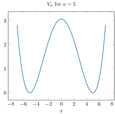
Figure 1. $x\mapsto V_{a}(x)$ for $a=1$ and $a=5$.

In practice, it is convenient to compute $\gamma_{a}$ and $E_{a}$ from the lowest two eigenvalues $\lambda_{a,1}<\lambda_{a,2}$ of $H_{a}$ and an associated pair $(\varphi_{a,1},\varphi_{a,2})$ of orthonormal eigenvectors

$$\begin{cases}\displaystyle H_{a}\varphi_{a,i}=\lambda_{a,i}\varphi_{a,i},\quad i=1,2\\ \displaystyle\langle\varphi_{a,i}|\varphi_{a,j}\rangle=\delta_{ij},\quad i,j=1,2,\end{cases}$$ (8)

$\langle\cdot|\cdot\rangle$ denoting the $L^{2}$ inner product. We indeed have

$$E_{a}=\lambda_{a,1}+\lambda_{a,2}\quad\mbox{and}\quad\gamma_{a}=|\varphi_{a,1}\rangle\langle\varphi_{a,1}|+|\varphi_{a,2}\rangle\langle\varphi_{a,2}|.$$ (9)

The evaluation of criteria $J_{A}$ and $J_{E}$ requires the computation of reference ground-state density matrices or energies, which amounts to find very accurate solutions of (8) for the configurations $a_{k}$ in the support of the chosen atomic probability measure

$$\mathbb{P}=\sum_{n=1}^{N_{\rm c}}w_{n}\delta_{a_{n}},\quad 0<a_{1}<a_{2}<\cdots<a_{N_{\rm c}},\quad w_{n}>0,\quad\sum_{n=1}^{N_{\rm c}}w_{n}=1.$$ (10)

We chose to compute these reference data using a 3-point finite-difference (FD) scheme on a large enough interval $[-x_{\rm max},x_{\rm max}]$ discretized into a uniform grid with $N_{g}$ grid points:

$$x_{j}=-x_{\rm max}+j\delta x,\quad 1\leqslant j\leqslant N_{g},\quad\delta x=\frac{2x_{\rm max}}{N_{g}+1}.$$

We then impose homogeneous Dirichlet boundary conditions at $-x_{\rm max}$ and $x_{\rm max}$. The parameter $x_{\rm max}$ is chosen such that $x_{\rm max}=a_{\rm max}+r_{\rm max}$, where $a_{\rm max}=\max(\mbox{supp}(\mathbb{P}))$ and $r_{\rm max}>0$ is is the radius beyond which atomic densities are zero at machine (double) precision. Note that this numerical scheme is independent of the configuration $a$. The FD discretization of problem (13) gives rise to the eigenvalue problem

$$\begin{cases}\displaystyle H_{a}^{\rm FD}\varphi_{a,i}^{FD}=\lambda_{a,i}^{\rm FD}\varphi_{a,i}^{\rm FD}\quad i=1,2\\ \delta x\bigl{(}\varphi_{a,i}^{\rm FD}\bigr{)}^{T}\varphi_{a,j}^{\rm FD}=\delta_{ij}^{\;},\end{cases}$$ (11)

where $H_{a}^{\rm FD}\in\mathbb{R}^{N_{g}\times N_{g}}_{\rm sym}$ is a real symmetric matrix of size $N_{g}\times N_{g}$, and the reference data are obtained as

$$E_{a}^{\rm FD}=\lambda_{a,1}^{\rm FD}+\lambda_{a,2}^{\rm FD}\quad\mbox{and}\quad P_{a}^{\rm FD}=\varphi_{a,1}^{\rm FD}\bigl{(}\varphi_{a,1}^{\rm FD}\bigr{)}^{T}+\varphi_{a,2}^{\rm FD}\bigl{(}\varphi_{a,2}^{\rm FD}\bigr{)}^{T}\in\mathbb{R}^{N_{g}\times N_{g}}_{\rm sym},$$ (12)

where $P_{a}^{\rm FD}$ can be interpreted as an approximation of the matrix $\gamma_{a}(x_{j},x_{j^{\prime}})$ containing the values of the (integral kernel of the) density matrix $\gamma_{a}$ at the grid points.

3.2. Variational approximation in AO basis sets

For any given configuration $a\in\mathbb{R}_{+}$ and basis $\chi=\{\chi_{\mu}\}_{1\leqslant\mu\leqslant N_{b}}\in\mathcal{B}$, problem (8) is solved using a Galerkin method with the basis $\chi_{a}=\{\chi_{a,\mu}\}_{1\leqslant\mu\leqslant 2N_{b}}$ composed of two copies of the basis $\chi$, the first one translated to $a$, and the second one to $-a$:

$$\chi_{a,1}=\chi_{1}(\cdot-a),\dots,\chi_{a,N_{b}}=\chi_{N_{b}}(\cdot-a),\;\chi_{a,N_{b}+1}=\chi_{1}(\cdot+a),\dots,\chi_{a,2N_{b}}=\chi_{N_{b}}(\cdot+a).$$

Defining the Hamiltonian matrix

$$H_{a}^{\chi}=\left(\left\langle\chi_{a,\mu}\biggl{|}\left(-\frac{1}{2}\frac{{\rm d}^{2}}{{\rm d}x^{2}}+V_{a}\right)\biggr{|}\chi_{a,\nu}\right\rangle\right)_{1\leqslant\mu,\nu\leqslant 2N_{b}}$$

and the overlap matrix

$$S^{\chi}_{a}=\left(\langle\chi_{a,\mu}|\chi_{a,\nu}\rangle\right)_{1\leqslant\mu,\nu\leqslant 2N_{b}},$$

the discretization of problem (8) in the AO basis set $\chi$ then reads as the generalized eigenvalue problem: find $\bigl{(}C_{a,i}^{\chi},\lambda_{a,i}^{\chi}\bigr{)}\in\mathbb{R}^{2N_{b}}\times\mathbb{R}$, $i=1,2$ such that

$$\begin{cases}\displaystyle H_{a}^{\chi}C_{a,i}^{\chi}=\lambda_{a,i}^{\chi}S^{\chi}_{a}C_{a,i}^{\chi}\quad i=1,2\\ \bigl{(}C_{a,i}^{\chi}\bigr{)}^{T}S^{\chi}_{a}C_{a,j}^{\chi}=\delta_{ij}.\end{cases}$$ (13)

The approximation $\varphi_{a,i}^{\chi}$ of $\varphi_{a,i}^{\,}$ in the AO basis set $\chi$ can then be recovered as the linear combination of atomic orbitals (LCAO)

$$\forall x\in\mathbb{R},\quad\varphi_{a,i}^{\chi}(x)=\sum\limits_{\mu=1}^{2N_{b}}[C_{a,i}^{\chi}]_{\mu}^{\,}\chi_{a,\mu}^{\,}(x).$$ (14)

One way to compare the LCAO ground-state 1-RDM to the reference FD solution $P_{a}^{\rm FD}$ is to simply evaluate the former at the grid points $x_{j}$, which gives rise to the matrix $P_{a}^{\chi}\in\mathbb{R}^{N_{g}\times N_{g}}_{\rm sym}$ with entries

$$[P_{a}^{\chi}]_{jj^{\prime}}=\sum_{i=1}^{2}\varphi_{a,i}^{\chi}(x_{j})\varphi_{a,i}^{\chi}(x_{j^{\prime}}).$$

Due to numerical errors, the matrix $P_{a}^{\chi}$ is however not a rank-2 orthogonal projector. We therefore chose to follow a slightly different route (leading to very similar results). The finite difference grid gives a reference discrete setting in which any quantity of interest for any configuration and AO basis set can be expressed. For all $a$’s, the basis $\chi_{a}$ is represented by a matrix $X_{a}\in\mathbb{R}^{N_{g}\times 2N_{b}}$. For any vectors $Y_{1},Y_{2}\in\mathbb{R}^{N_{g}}$, the discrete $A$ inner product simply reads $\delta xY_{1}^{T}AY_{2}^{\,}$ where the notation $A$ stands for both the continuous inner product and its finite-difference discretization matrix. We denote by $\|\cdot\|_{A}$ the associated norm on $\mathbb{R}^{N_{g}}$. Solutions to (13) are then obtained by approximating respectively the Hamiltonian and overlap matrix by

$$H_{a}^{\chi}\simeq H_{a}^{X}\coloneqq\left(\delta xX_{a,\mu}^{T}H_{a}^{\rm FD}X_{a,\nu}^{\,}\right)_{1\leqslant\mu,\nu\leqslant 2N_{b}},\quad S^{\chi}_{a}\simeq S^{X}_{a}\coloneqq\left(\delta xX_{a,\mu}^{T}X_{a,\nu}^{\,}\right)_{1\leqslant\mu,\nu\leqslant 2N_{b}},$$

and finding $(C_{a,i}^{X},\lambda_{a,i}^{X})\in\mathbb{R}^{2N_{b}}\times\mathbb{R}$, $i=1,2$, such that

$$\left\{\begin{array}[]{l}\displaystyle H_{a}^{X}C_{a,i}^{X}=\lambda^{X}_{a,i}S^{X}_{a}C_{a,i}^{X},\quad i=1,2\\ \\ (C_{a,i}^{X})^{T}S^{X}_{a}C_{a,j}^{X}=\delta_{ij}^{\;},\quad i,j=1,2,\end{array}\right.$$ (15)

from which we get the discrete approximations

$${\varphi}_{a,i}^{X}=X_{a}^{\,}C_{a,i}^{X},\quad i=1,2.$$ (16)

Let us gather the coefficients ${C}_{a,i}^{X}$ into the $2N_{b}\times 2$ matrix ${C}_{a}^{X}=\left(\,C_{a,1}^{X}\,|\,C_{a,2}^{X}\,\right)$. The ground-state density matrix in the basis $\chi_{a}$ is approximated by

$${P}_{a}^{X}={\varphi}_{a,1}^{X}({\varphi}_{a,1}^{X})^{T}+{\varphi}_{a,2}^{X}({\varphi}_{a,2}^{X})^{T}=\left(X_{a}^{\,}{C}^{X}_{a}\right)\left(X_{a}^{\,}{C}^{X}_{a}\right)^{T}\in\mathbb{R}^{N_{g}\times N_{g}}_{\rm sym}.$$ (17)

3.3. Overcompleteness of Hermite Basis Sets

Before getting into basis set optimization, we introduce the following standard Hermite Basis Set (HBS), constructed from eigenfunctions of the quantum harmonic oscillator. Those functions are solutions to the eigenvalue problem $\left(-\frac{1}{2}\frac{{\rm d}^{2}}{{\rm d}x^{2}}+\frac{1}{2}x^{2}\right)h_{n}=\varepsilon_{n}h_{n}$ and are explicitly given by

$$h_{n}(x)=c_{n}p_{n}(x)\exp\left({-\frac{x^{2}}{2}}\right),\quad\varepsilon_{n}=n+\frac{1}{2},\quad n\in\mathbb{N},$$ (18)

where $p_{n}$ is the Hermite polynomial of degree $n$ (with the same parity as $n$) and $c_{n}$ a normalization constant such that $(h_{n})_{n\in\mathbb{N}}$ forms an orthonormal basis of $L^{2}(\mathbb{R})$. The $h_{n}$’s are the analogues of the standard atomic orbitals obtained by solving atomic electronic structure problems. Let us first consider the AO basis set made of the first $N_{b}$ Hermite functions

$$\chi^{\rm HBS}=\{\chi_{\mu}^{\rm HBS}\}_{1\leqslant\mu\leqslant N_{b}}=\{h_{n}\}_{0\leqslant n\leqslant N_{b}-1}.$$

The overlap matrix for the configuration $a$ then is of the form

$$S_{a}^{\chi^{\rm HBS}}=\begin{pmatrix}I_{N_{b}}&\Sigma_{a}\\[2.84544pt] \Sigma_{a}^{T}&I_{N_{b}}\end{pmatrix}\quad\text{where}\quad\Sigma_{a}\coloneqq(\langle h_{n}(\cdot-a)|h_{m}(\cdot+a)\rangle)_{0\leqslant n,m\leqslant N_{b}-1}.$$

The matrix $\Sigma_{a}$ corresponds to the overlap of functions that are localized at different atomic positions. It satisfies $\Sigma_{a}\simeq 0$ when $a$ is large and $\Sigma_{a}\simeq I_{N_{b}}$ when $a$ is close to 0, therefore causing conditioning issues on the overlap matrix $S_{a}^{\chi^{\rm HBS}}$, a phenomenon known as overcompleteness: when $a$ is too small, the basis functions centered at $\pm a$ are almost equal, hence almost linearly dependent in the basis set. We illustrate this problem by plotting the condition number of the overlap matrix $S_{a}^{\chi^{\rm HBS}}$ for different values of $a$ in Figure 2, which indeed blows up for small values of $a$.

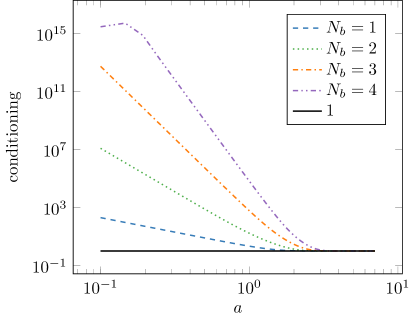
Figure 2. Condition number of the HBS overlap matrix $S_{a}^{\chi^{\rm HBS}}$ for different values of $a$ in log-log scale. The larger the basis set, the faster the condition number blows up for small values of $a$.

3.4. Practical computation of the criterion $J_{A}$ and $J_{E}$

The rest of this section is dedicated to the rewriting and the computation of criteria $J_{A}$ and $J_{E}$ for our 1D model in the discrete setting.

3.4.1. Reference orthonormal basis

In order to avoid potential numerical stability issues, each of the $N_{b}$ atomic orbital $\chi_{\mu}$ is decomposed on a given truncated orthonormal basis of $L^{2}(\mathbb{R})$ of size $\mathcal{N}$ such that $N_{b}\ll\mathcal{N}\ll N_{g}$. We choose here the orthonormal basis introduced in (18). Hence, the matrix $X_{a}\in\mathbb{R}^{N_{g}\times 2N_{b}}$ is written as

$$X_{a}=B_{a}I_{R},$$ (19)

with

$$B_{a}=\begin{pmatrix}h_{0}(x_{\cdot}-a)|\cdots|h_{\mathcal{N}-1}(x_{\cdot}-a)|h_{0}(x_{\cdot}+a)|\cdots|h_{\mathcal{N}-1}(x_{\cdot}+a)\end{pmatrix}\in\mathbb{R}^{N_{g}\times 2\mathcal{N}},$$

and

$$I_{R}=\begin{pmatrix}R&0\\ 0&R\end{pmatrix}\in\mathbb{R}^{(2\mathcal{N})\times(2N_{b})},$$ (20)

where $R\in\mathbb{R}^{\mathcal{N}\times N_{b}}$ gathers the coefficients of the atomic orbitals $\chi_{\mu}$ in the truncated HBS orthonormal basis. Note that we have duplicated $R$ in $I_{R}$ as we consider the same basis at each position $\pm a$, but everything that follows can be easily adapted to the case where we would like to optimize the bases at each position separately (to deal with heteronuclear molecular systems for instance). We moreover impose that $R^{T}R=I_{N_{b}}$, so that the overlap matrix of $X_{a}$, denoted by $S(X_{a})$, has the same form as in Section 3.3, that is

$$S(X_{a})\coloneqq\delta xX_{a}^{T}X_{a}^{\,}=\begin{pmatrix}I_{N_{b}}&\Sigma_{a}\\ \Sigma_{a}^{T}&I_{N_{b}}\end{pmatrix},$$ (21)

where $\Sigma_{a}$ is the overlap between functions localized at $+a$ and functions localized at $-a$. To avoid any issues arising from the conditioning of $S({X_{a}})$, the minimal sampled distance $a_{\rm min}$ should not be taken too small.

In the following, we detail the computation of each of the two criteria using the matrix $R$ as the main variable. We will subsequently optimize the criteria $J_{A}$ and $J_{E}$ with respect to $R$ to obtain optimal AO basis sets. In order to ease the reading of the following computations, every vector of $\mathbb{R}^{N_{g}}$ is rescaled by a factor $\sqrt{\delta x}$ so that for any given $Y_{1},Y_{2}\in\mathbb{R}^{N_{g}}$ the discrete $A$ inner product simply reads $Y_{1}^{T}AY_{2}^{\,}$. The same holds for overlap matrices: with this convention, $S(X_{a})=X_{a}^{T}X_{a}^{\,}$. The output of the optimization is then scaled back to its former state by a factor $1/\sqrt{\delta x}$ to recover the original normalization.

3.4.2. Criterion $J_{A}$

Let $a\in\mathbb{R}_{+}$ be fixed and let $S^{A}(Y)=Y^{T}AY$ denote the overlap matrix for the $A$-inner product of any rectangular matrix $Y\in\mathbb{R}^{N_{g}\times d}$. Since the columns of ${X_{a}}[S^{A}(X_{a})]^{-\frac{1}{2}}$ are orthonormal for the $A$ inner product, that is

$$\left({X_{a}}[S^{A}(X_{a})]^{-\frac{1}{2}}\right)^{T}A\left({X_{a}}[S^{A}(X_{a})]^{-\frac{1}{2}}\right)=I,$$

the projection $\Pi_{X_{a}}^{A}$ takes the simple form

$$\Pi_{X_{a}}^{A}=\left({X_{a}}[S^{A}({X_{a}})]^{-\frac{1}{2}}\right)\left({X_{a}}[S^{A}({X_{a}})]^{-\frac{1}{2}}\right)^{T}A=X_{a}[S^{A}({X_{a}})]^{-1}X_{a}^{T}A.$$ (22)

Hence, using the cyclicity of the trace and definitions (3), (12) and (22), one has

$$j_{A}(\chi,a) \simeq-{\rm Tr}\left(P_{a}^{\rm FD}\,\Pi_{X_{a}}^{A}A\Pi_{X_{a}}^{A}\right)$$

$$=-{\rm Tr}\left(P_{a}^{\rm FD}\times(AB_{a}I_{R}^{\,})[S^{A}(B_{a}I_{R}^{\,})]^{-1}(AB_{a}I_{R}^{\,})^{T}\right)$$

$$=-{\rm Tr}\left(M^{\rm offline}_{A}(a)I_{R}^{\,}[S^{A}(B_{a}I_{R}^{\,})]^{-1}I_{R}^{T}\right),$$

where we have collected in the last expression all matrices independent of $R$ into the matrix

$$M^{\rm offline}_{A}(a)=(AB_{a})^{T}P_{a}^{\rm FD}AB_{a}\in\mathbb{R}^{2\mathcal{N}\times 2\mathcal{N}}.$$ (23)

Then, using the probability measure $\mathbb{P}$ in (10), we get

$$J_{A}(R)=-\int_{\Omega}{\rm Tr}\left(M^{\rm offline}_{A}(a)I_{R}^{\,}[S^{A}(B_{a}^{\,}I_{R}^{\,})]^{-1}I_{R}^{T}\right)\,{\rm d}\mathbb{P}(a)=-\sum_{n=1}^{N_{\rm c}}w_{n}{\rm Tr}\left(M^{\rm offline}_{A}(a_{n})I_{R}^{\,}[S^{A}(B_{a_{n}}^{\,}I_{R}^{\,})]^{-1}I_{R}^{T}\right)$$

and the optimization problem finally writes, with unknown $R\in\mathbb{R}^{\mathcal{N}\times N_{b}}$ and for a given inner product $A$

$$\boxed{\mbox{Find }R_{\rm opt}\in\underset{R\in\mathbb{R}^{\mathcal{N}\times N_{b}},\ R^{T}R=I_{N_{b}}}{\rm argmin}J_{A}(R)}$$ (24)

3.4.3. Criterion $J_{E}$

Let again $a\in\mathbb{R}_{+}$ be fixed. We denote by

$$G(N_{g},2)\coloneqq\{P\in\mathbb{R}^{N_{g}\times N_{g}}\,|\,P^{2}=P=P^{T},{\rm Tr}(P)=2\}$$

the discrete counterpart of the Grassmann manifold $\mathcal{G}_{2}$, and write $E_{a}^{R}$ (resp. $H_{a}^{R}$) instead of $E_{a}^{\chi}$ (resp. $H_{a}^{\chi}$), so that the dependence in the matrix $R$ appears explicitly. Equation (7) reads in the discrete setting

$$\begin{split}E_{a}^{R}=\displaystyle{\min_{P\in\,G(N_{g},2)}{\rm Tr}\left(PH_{a}^{R}\right)}&=\displaystyle{\min_{\begin{subarray}{c}C\in\mathbb{R}^{2N_{b}\times 2}\\ (C)^{T}S(B_{a}I_{R})C=I_{2}\end{subarray}}{\rm Tr}\left(CC^{T}\times(B_{a}I_{R})^{T}H_{a}^{\rm FD}(B_{a}I_{R})\right)}\\ &={\rm Tr}\left(C_{a}^{R}(C_{a}^{R})^{T}\times I_{R}^{T}M^{\rm offline}_{E}(a)I_{R}^{\,}\right)\end{split}$$ (25)

where, as for the previous case, all matrices independent of $R$ have been gathered in the matrix

$$M^{\rm offline}_{E}(a)=B_{a}^{T}H_{a}^{\rm FD}B_{a}^{\,},$$ (26)

and the matrix $C_{a}^{R}$ is solution to the minimization problem

$${\min_{\begin{subarray}{c}C^{R}\in\mathbb{R}^{2N_{b}\times 2}\\ (C^{R})^{T}S(B_{a}I_{R})C^{R}=I_{2}\end{subarray}}{\rm Tr}\left(C^{R}(C^{R})^{T}\times I_{R}^{T}M_{E}^{\rm offline}(a)I_{R}\right)}$$ (27)

and is given in practice by $C_{a}^{R}=\left[S(B_{a}I_{R})\right]^{-\tfrac{1}{2}}(u_{a,1}|u_{a,2})$ where $u_{a,1}$ and $u_{a,2}$ are orthonormal eigenvectors associated to the lowest two eigenvalues of

$$\left[S(B_{a}I_{R})\right]^{-\tfrac{1}{2}}I_{R}^{\,}M^{\rm offline}_{E}(a)I_{R}^{T}\left[S(B_{a}I_{R})\right]^{-\tfrac{1}{2}}.$$

From (10) and (25), one can compute

$$J_{E}(R)=\int_{\Omega}\left|E_{a}^{\rm FD}-E_{a}^{R}\right|^{2}\,{\rm d}\mathbb{P}(a)=\sum_{n=1}^{N_{\rm c}}w_{n}\left|E_{a_{n}}^{\rm FD}-E_{a_{n}}^{R}\right|^{2}$$

and the optimization problem reads

$$\boxed{{\rm Find}\;R_{\rm opt}\in\underset{R\in\mathbb{R}^{\mathcal{N}\times N_{b}},\ R^{T}R=I_{N_{b}}}{\rm argmin}J_{E}(R)}$$ (28)

4. Numerical results

4.1. Numerical setting and first results

Problems (24) and (28) are solved by direct minimization algorithms over the Stiefel manifold [1]

$${\rm St}(\mathcal{N},N_{b})=\{R\in\mathbb{R}^{\mathcal{N}\times N_{b}}\,|\,R^{T}R=I_{N_{b}}\}.$$

The explicit computation of the gradients of $J_{A}$ and $J_{E}$ with respect to $R$ is detailed in the Appendix. We used a L–BFGS algorithm (with tolerance $10^{-7}$ on the norm of the projected gradient), as implemented in the Optim.jl package [19] in the Julia language [4]. As initial guess, we picked the first $N_{b}$ Hermite functions introduced in Section 3.3.

In this subsection, we choose a probability distribution $\mathbb{P}$ supported in the interval $\mathcal{I}=[1.5,5]$ so as to retain the physics of interest that takes place around the equilibrium configuration $a_{0}\simeq 1.925$ and all the way to dissociation. In particular $a_{\rm min}=1.5$ is taken sufficiently large to avoid the conditioning issues on the overlap matrices described in Section 3.3. More precisely, all the results in this subsection are obtained with the probability

$$\mathbb{P}=\frac{1}{10}\sum_{n=1}^{10}\delta_{a_{n}}\quad\mbox{with }a_{n}=1.5+(n-1)\frac{3.5}{9}.$$ (29)

The quantities $M^{\rm offline}_{A}(a_{n})$ and $M^{\rm offline}_{E}(a_{n})$ are computed offline beforehand. We will discuss this choice and consider other probability measures $\mathbb{P}$ in Sections 4.2.2 and 4.2.3.

The finite-difference grid is a uniform grid on the interval $[-20,20]$ discretized into $N_{g}=1999$ points ($\delta x=0.02$). Finally, we decompose the basis functions to be optimized in the HBS $\{h_{n}\}_{0\leqslant n\leqslant\mathcal{N}-1}$ of $L^{2}(\mathbb{R})$ of size $\mathcal{N}=10$. Regarding the choice of the inner product for the first criterion $J_{A}$, we used the standard $L^{2}(\mathbb{R})$ and the $H^{1}(\mathbb{R})$ inner products, and denoted $J_{L^{2}}$ and $J_{H^{1}}$ the corresponding. This translates at the discrete level by choosing $A=I_{N_{g}}$ for $J_{L^{2}}$ and $A=I_{N_{g}}-\Delta$ for $J_{H^{1}}$ where $\Delta$ is the 3-point finite-difference discretization matrix of the 1D Laplace operator. Once obtained, the optimal bases are used to solve the variational problem (15) on a much finer sampling of $\mathcal{I}$ and their accuracy is compared to the HBS. The code performing the simulations and plotting the results is available online. Also, for the sake of clarity in the plots, $\widetilde{E}_{a}$ (resp. $\widetilde{\rho}_{a}$) denotes the GS energy (resp. the density) in the configuration $a$ with a given basis (specified by the context) and $E_{a}$ (resp. $\rho_{a}$) stands for the reference energy (resp. density) on the finite difference grid. Note that we write HBS for the (nonoptimized) Hermite basis set, and $L^{2}$-OBS, $H^{1}$-OBS or $E$-OBS for optimized basis sets with respect to the criterion $J_{L^{2}}$, $J_{H^{1}}$, or $J_{E}$.

Figure 3 displays the dissociation curve and the energy difference on the interval $\mathcal{I}$ for different values of $N_{b}$, the size of the AO basis set. For $N_{b}=1$, i.e. only one basis function at $\pm a$, criterion $J_{E}$ shows better performance than the criterion $J_{A}$, regardless of the choice of norm to perform the projections. It also very closely matches the accuracy of the standard HBS. When $N_{b}$ becomes larger however, the different criteria behave in a similar fashion and we observe that they approach the dissociation curve better than the Hermite basis. Comparing the values of criterion $J_{E}$ for all bases, which directly measures the distance to the dissociation curve, we see in Table 1 that all optimized bases give an increased accuracy of roughly four orders of magnitude over the interval $\mathcal{I}$ for $N_{b}=4$.

In Figure 4, we plot the density for a given value of $a$ and the error on the density for different norms, with varying values of $N_{b}$. The error is plotted with respect to three different distances: the $L^{1}$-norm, which corresponds to the $L^{2}$-norm on eigenvectors, the $H^{1}$-norm of the error on the density, as it is common to compute the forces $\int_{\mathbb{R}}\rho\nabla_{a}V_{a}$ with good estimates on the $H^{-1}$-norm of $\nabla_{a}V_{a}$ (see e.g. [8]), and the distance

$$\|\nabla\sqrt{\rho_{1}}-\nabla\sqrt{\rho_{2}}\|_{L^{2}}$$

(recall that the von-Weizsäcker kinetic energy reads $\frac{1}{2}\int_{\mathbb{R}}|\nabla\sqrt{\rho}|^{2}$). We observe similar behaviors between these different distances. For $N_{b}=1$, both bases obtained with the first criterion behave slightly better than the standard Hermite basis and the basis computed with the second criterion. For $N_{b}=3$, we observe again that all optimal bases yield better accuracy than the Hermite basis. Table 1 gives the confirmation that each basis for a given criterion indeed performs better than the other bases for that particular criterion. As for dissociation curves, we read from the values of $J_{L^{2}}$ and $J_{H^{1}}$ that the optimized bases yield similar results for large $N_{b}$, all of them giving lower values than the HBS. Note that the optimal bases for criterion $J_{L^{2}}$ and $J_{H^{1}}$ give similar results for any number of basis functions $N_{b}$, so that the $L^{2}$ and $H^{1}$ norm optimizations seem equivalent.

In terms of computational time, first note that criterion $J_{H^{1}}$ is always more expensive to compute than $J_{L^{2}}$ as it requires additional matrix-vector products with the matrix $A$, this having noticeable impact on the computational time. Second, criterion $J_{E}$ requires less off-line data as it only needs to be given the reference eigenvalues while criterion $J_{A}$ requires the reference GS eigenvectors (or density matrices). This also influences the computational time. Indeed, regarding timings, criterion $J_{E}$ is about 10 times faster to minimize than criterion $J_{L^{2}}$ norm in our implementation.

Finally, for the sake of completeness, we plot in Figure 5 the different basis functions built with each criterion for different values of $N_{b}$, confirming again the previous observations that the optimal basis functions are quite close to the standard Hermite basis functions.

The main conclusion of these observations is that, for $N_{b}$ large enough, there is no real difference between the proposed criteria. Still, if the bases we built do not seem to be very different from the standard Hermite basis (Figure 5), building optimal bases allows to increase accuracy on the quantities of interest we focused on by one order of magnitude in average.

Value of $J_{L^{2}}$ for the different basis sets		Value of $J_{H^{1}}$ for the different basis sets
Basis $N_{b}=1$ $N_{b}=2$ $N_{b}=3$ $N_{b}=4$ HBS -7.40829 -7.70051 -7.74312 -7.77138 $L^{2}$-OBS -7.43954 -7.76479 -7.77725 -7.77773 $H^{1}$-OBS -7.43928 -7.76466 -7.77724 -7.77772 E-OBS -7.39410 -7.76425 -7.77720 -7.77772		Basis $N_{b}=1$ $N_{b}=2$ $N_{b}=3$ $N_{b}=4$ HBS -10.5613 -11.0566 -11.1451 -11.2402 $L^{2}$-OBS -10.6256 -11.2338 -11.2630 -11.2650 $H^{1}$-OBS -10.6265 -11.2342 -11.2630 -11.2651 E-OBS -10.5334 -11.2313 -11.2626 -11.2650

Value of $J_{E}$ for the different basis sets

Basis $N_{b}=1$ $N_{b}=2$ $N_{b}=3$ $N_{b}=4$ HBS 3.77956$\times 10^{-2}$ 3.98301$\times 10^{-3}$ 1.86537$\times 10^{-3}$ 1.35309$\times 10^{-4}$ $L^{2}$-OBS 6.52016$\times 10^{-2}$ 2.18282$\times 10^{-4}$ 1.01365$\times 10^{-6}$ 3.22260$\times 10^{-8}$ $H^{1}$-OBS 6.83537$\times 10^{-2}$ 2.40548$\times 10^{-4}$ 1.27251$\times 10^{-6}$ 3.91885$\times 10^{-8}$ E-OBS 3.69610$\times 10^{-2}$ 1.92087$\times 10^{-4}$ 6.93394$\times 10^{-7}$ 2.54014$\times 10^{-8}$

L–BFGS iterations

Basis $N_{b}=1$ $N_{b}=2$ $N_{b}=3$ $N_{b}=4$ $L^{2}$-OBS 4 13 48 219 $H^{1}$-OBS 7 17 235 not converged after 500 it E-OBS 6 19 52 134

Table 1. (Top & Middle) Values of the different criteria for the HBS and optimal bases, for increasing values of $N_{b}$. (Bottom) Number of iterations of L–BFGS required for each criterion to achieve convergence up to requested tolerance ($10^{-7}$ on the $\ell^{2}$-norm of the gradient).

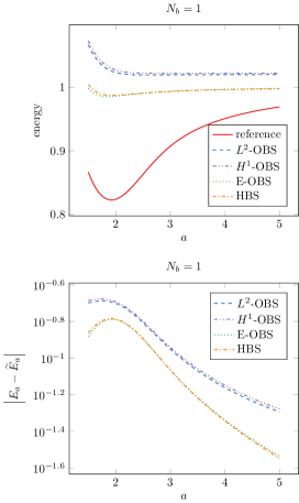
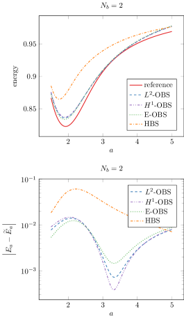
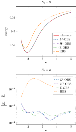
Figure 3. Energies for the optimal bases obtained with the different criteria. (Top) Dissociation curve. (Bottom) Errors on the energy on the range of configuration $\mathcal{I}=[1.5,5]$.

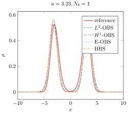
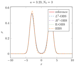
e

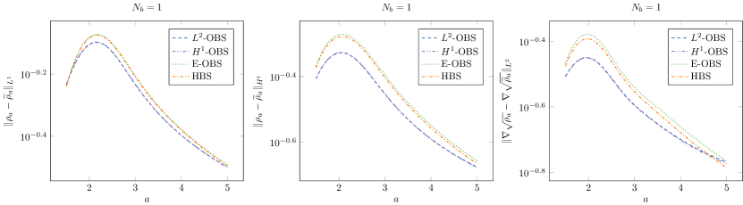
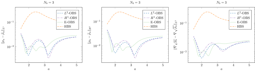
Figure 4. (Top) Densities for the optimal bases obtained with the different criteria. (Middle) Errors on the density for different norms with $N_{b}=1$. (Bottom) Error on the density for different norms with $N_{b}=3$.

$N_{b}=1$

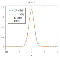
$N_{b}=2$

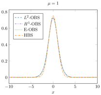
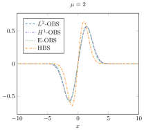
$N_{b}=3$

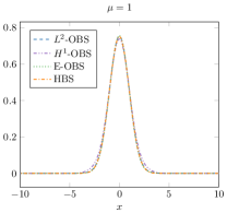
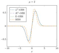
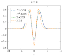
$N_{b}=4$

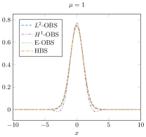
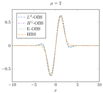
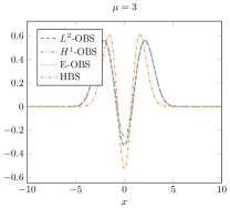
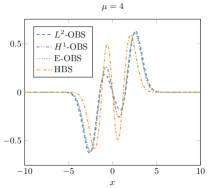
Figure 5. Optimal basis functions for different criteria, each of them being optimized for different values of $N_{b}$.

4.2. Influence of numerical parameters

4.2.1. Random starting points

In Section 4.1, we used the first $N_{b}$ Hermite functions as a starting point for the optimization procedures. We obtain the same solutions if we start from a random matrix $R$ on the Stiefel manifold, in the sense that the optimal values reached for each criterion are the same, as well as the error plots. However, the L–BFGS algorithm requires more iterations to converge. The basis functions obtained from the optimization algorithms are different from those observed in Figure 5, but still span the same space as the variational solutions are equal.

4.2.2. Extrapolating the parameter space $\mathcal{I}$

In Section 4.1, we chose a probability measure $\mathbb{P}$ supported in the interval $[1.5,5]$ in order to avoid conditioning issues. Indeed, taking smaller values of $a$ results in the L–BFGS algorithm having convergence problems when $N_{b}$ increases. This phenomenon was observed already for $N_{b}=3$ or $N_{b}=4$ when including $a=1$ in the support of $\mathbb{P}$. In practice, this problem can be solved by using preconditioning or getting rid of overcompleteness by pre-processing the basis $\chi_{a}$ (e.g. selecting a smaller basis by filtering out the very small singular values of the original overlap matrix), but for brevity we will not elaborate further in this direction.

However, once we have computed optimal bases for a reasonable interval $\mathcal{I}$, it is possible to use these bases to solve the variational problem (13) and extrapolate the energy and the density to smaller values of $a$ that are not in the set $\mathcal{I}$. The results are plotted in Figure 6. We notice that the quantities of interest are better approximated on $\mathcal{I}=[1.5,5]$, but for smaller $a$’s, there is no more gain in accuracy with respect to the standard HBS.

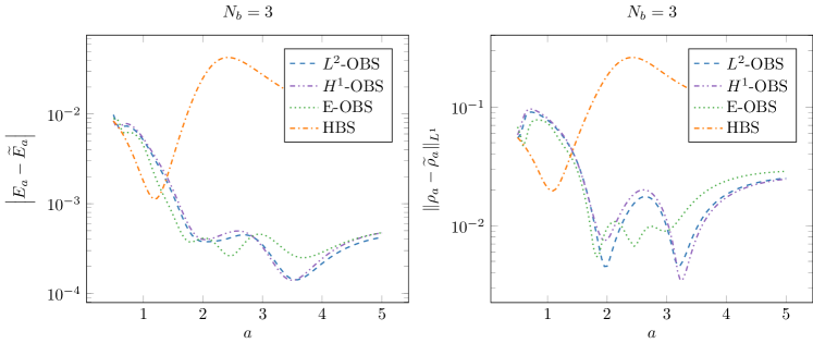
Figure 6. Energy and densities error with extrapolation up to $a=0.5$, with basis functions optimized on $\mathcal{I}=[1.5,5]$

.

4.2.3. Choice of the probability $\mathbb{P}$

The major drawback of our AO basis optimization lies in the necessity to compute very accurate reference solutions for all configurations in the support of $\mathbb{P}$. This is not an issue for our 1D toy model but it can be very time consuming for real systems if the support of $\mathbb{P}$ is too large. It is therefore crucial to reduce as much as possible the support of $\mathbb{P}$.

In this section, we study the influence of the probability measure $\mathbb{P}$ on the quality of the optimized bases. For simplicity, we restrict ourselves to uniform samplings of the interval $\mathcal{I}=[1.5,5]$. Numerical tests show that increasing the sample size above the reference sampling with $N_{\rm c}=10$ points used in Section 4.1 (see Eq. (29)) brings no significant accuracy improvement. Therefore we chose to investigate in the following the performance of the optimal AO basis sets obtained with very sparse sampling. Figure 7 pictures the error of approximation of the dissociation curve and densities for three samplings: first, the two extreme points of the interval $\mathcal{I}=[1.5,5]$; second, two points around the equilibrium distance $a_{0}\simeq 1.925$ ; third, a single point near the equilibrium distance. All curves are plotted for a fixed number of basis functions $N_{b}=3$.

It appears that the latter sampling already provides satisfactory accuracy. The criteria $J_{L^{2}}$ and $J_{H^{1}}$ are equal to $-5\times 10^{-6}$ for optimized basis to be compared with $-1.8\times 10^{-3}$ for standard HBS. Hence they provide a gain of accuracy in energy of three orders of magnitude over the whole dissociation curve.

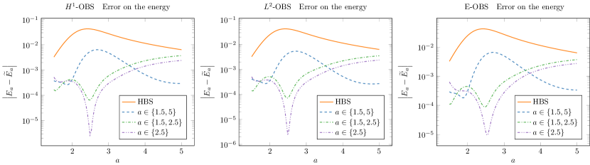
Figure 7. Error plots for probability measures $\mathbb{P}$ corresponding to very sparse samplings of the interval $\mathcal{I}=[1.5,5]$: i) the two endpoints of $\mathcal{I}$ ii) two points near the equilibrium distance and iii) one point near the equilibrium distance. (Top line) Error on energy. (Bottom line) Error on density in $L^{1}$ norm. (Left) OBS for $J_{H^{1}}$. (Middle) OBS for $J_{L^{2}}$. (Right) OBS for $J_{E}$. The “$a$” in legends are the sampled configurations $a$.

4.2.4. Number of Hilbert basis functions

We now take the same setting as in Section 4.1, except that we set $\mathcal{N}=5$ instead of $\mathcal{N}=10$. This provides similar results as those collected in Table 1, see Table 2. However, the values of the criteria $J_{A}$ and $J_{E}$ are higher than for $\mathcal{N}=10$, in particular for $N_{b}=4$, where criterion $J_{A}$ cannot be optimized further than $-10^{-5}$, which makes sense as the space over which the optimization algorithms are performed is smaller. Calculations with $\mathcal{N}=15$ were also performed: for $N_{b}=1,2,3$, the criteria are slightly improved but for $N_{b}=4$, convergence issues were noticed, due to ill conditioning of the overlap matrices for $a=1.5$ as the number $\mathcal{N}$ of functions used to describe the optimal bases is larger.

Value of $J_{L^{2}}$ for the different basis sets		Value of $J_{H^{1}}$ for the different basis sets
Basis $N_{b}=1$ $N_{b}=2$ $N_{b}=3$ $N_{b}=4$ HBS -7.40829 -7.70051 -7.74312 -7.77138 $L^{2}$-OBS -7.43933 -7.76304 -7.77554 -7.77618 $H^{1}$-OBS -7.43923 -7.76258 -7.77525 -7.77612 E-OBS -7.39401 -7.76259 -7.77545 -7.77615		Basis $N_{b}=1$ $N_{b}=2$ $N_{b}=3$ $N_{b}=4$ HBS -10.5613 -11.0566 -11.1451 -11.2402 $L^{2}$-OBS -10.6237 -11.2225 -11.2541 -11.2577 $H^{1}$-OBS -10.6240 -11.2244 -11.2555 -11.2581 E-OBS -10.5328 -11.2234 -11.2547 -11.2580

Value of $J_{E}$ for the different basis sets

Basis $N_{b}=1$ $N_{b}=2$ $N_{b}=3$ $N_{b}=4$ HBS 3.77956$\times 10^{-2}$ 3.98301$\times 10^{-3}$ 1.86537$\times 10^{-3}$ 1.35309$\times 10^{-4}$ $L^{2}$-OBS 6.43832$\times 10^{-2}$ 2.46466$\times 10^{-4}$ 1.58667$\times 10^{-5}$ 1.01128$\times 10^{-5}$ $H^{1}$-OBS 6.13025$\times 10^{-2}$ 2.45930$\times 10^{-4}$ 1.62235$\times 10^{-5}$ 1.00611$\times 10^{-5}$ E-OBS 3.69681$\times 10^{-2}$ 1.30365$\times 10^{-4}$ 1.41935$\times 10^{-5}$ 9.74560$\times 10^{-6}$

Table 2. Value of the different criteria for the different local (optimized and Hermite) bases, with $\mathcal{N}=5$ and increasing values of $N_{b}$.

Appendix

In this appendix, we will use extensively the two symmetries of the trace: for any matrices $M$ and $N$ such that $MN$ and $NM$ are defined,

$${\rm Tr}(MN)={\rm Tr}(NM)\quad\mbox{and}\quad{\rm Tr}(M^{T})={\rm Tr}(M).$$

Computation of the gradient of $J_{A}$

Let $R,H\in\mathbb{R}^{\mathcal{N}\times N_{b}}$ and define $I_{H}=\begin{pmatrix}H&0\\ 0&H\end{pmatrix}$. One has

$$\begin{split}J_{A}(R+H)-J_{A}(R)&=-\int_{\Omega}{\rm Tr}\left(M_{A}^{\rm offline}(a)\left(2I_{R}[S^{A}(B_{a}I_{R}^{\,})]^{-1}I_{H}^{T}+I_{R}^{\,}\,\left[{\rm d}[S^{A}]^{-1}(B_{a}I_{R})\cdot(B_{a}I_{H}^{\,})\right]I_{R}^{T}\right)\right)\,{\rm d}\mathbb{P}(a)\\ &+O(\|H\|^{2})\end{split}$$ (30)

Considering that

$$(M+H)^{-1}-M^{-1}=-M^{-1}HM^{-1}+O(\|H\|^{2})\mbox{ and }S^{A}(BI_{R+H})-S^{A}(B_{a}I_{R})=I_{H}^{T}S^{A}(B)I_{R}^{\,}+I_{R}^{T}S^{A}(B)I_{H}^{\,}+O(\|H\|^{2}),$$

it follows from the chain rule that

$${\rm d}[S^{A}]^{-1}(B_{a}I_{R})\cdot(B_{a}I_{H}) =-[S^{A}(B_{a}I_{R})]^{-1}\left(I_{H}^{T}S^{A}(B_{a})I_{R}^{\,}+I_{R}^{T}S^{A}(B_{a})I_{H}^{\,}\right)[S^{A}(B_{a}I_{R})]^{-1}.$$

From this computation, we obtain that the integrand in expression (30) writes for all $a$

$$2{\rm Tr}\left(M_{A}^{\rm offline}(a)\left[I_{R}[S^{A}(B_{a}I_{R}^{\,})]^{-1}I_{H}^{T}-I_{R}[S^{A}(B_{a}I_{R})]^{-1}I_{H}^{T}S^{A}(B_{a})I_{R}^{\,}[S^{A}(B_{a}I_{R})]^{-1}I_{R}^{T}\right]\right)$$

$$=2{\rm Tr}\left(M_{A}^{\rm offline}(a)I_{R}[S^{A}(B_{a}I_{R}^{\,})]^{-1}I_{H}^{T}-I_{H}^{T}S^{A}(B_{a})I_{R}^{\,}[S^{A}(B_{a}I_{R})]^{-1}I_{R}^{T}M_{A}^{\rm offline}(a)I_{R}[S^{A}(B_{a}I_{R})]^{-1}\right).$$ (31)

The idea is now to write the expression (Computation of the gradient of $J_{A}$) as the inner product of $H$ with a given matrix of $\mathbb{R}^{\mathcal{N}\times N_{b}}$, which we will identify as the integrand of the gradient of $K_{I}$. Changing from $I_{H}$ to $H$ imposes to decompose each matrix by block and to write the trace in (Computation of the gradient of $J_{A}$) as the sum of traces over the diagonal blocks. To this end we introduce the superscripts "$++$", "$+-$", "$-+$" and "$--$" associated with one of the four identically shaped blocks of a generic matrix

$$M=\begin{pmatrix}M^{++}&M^{+-}\\ M^{-+}&M^{--}\end{pmatrix}.$$ (32)

Expression (Computation of the gradient of $J_{A}$) therefore immediately reads

$$2{\rm Tr}\biggl{(}I_{H}^{T}\underbrace{\left[M_{A}^{\rm offline}(a)I_{R}^{\,}[S^{A}(B_{a}I_{R}^{\,})]^{-1}-S^{A}(B_{a})I_{R}^{\,}[S^{A}(B_{a}I_{R})]^{-1}I_{R}^{T}M_{A}^{\rm offline}(a)I_{R}[S^{A}(B_{a}I_{R})]^{-1}\right]}_{\displaystyle M_{A}(a,R)}\biggr{)}$$

$$\hskip 56.9055pt=2{\rm Tr}\left(H^{T}\left(M_{A}(a,R)^{++}+M_{A}(a,R)^{--}\right)\right).$$ (33)

One can verify that $M_{A}(a,R)^{++}+M_{A}(a,R)^{--}$ is in $\mathbb{R}^{\mathcal{N}\times N_{b}}$ and we conclude by identification that

$$\boxed{\nabla J_{A}(R)=-2\int_{\Omega}\left(M_{A}(a,R)^{++}+M_{A}(a,R)^{--}\right){\rm d}\mathbb{P}(a).}$$ (34)

Computation of the gradient of $J_{E}$

Let $R,H\in\mathbb{R}^{\mathcal{N}\times N_{b}}$ and define $I_{H}=\begin{pmatrix}H&0\\ 0&H\end{pmatrix}$. We immediately have that

$$\nabla J_{E}(R)=-2\int_{\Omega}\nabla E_{a}(R)\left(E_{a}^{\,}-E_{a}(R)\right){\rm d}\mathbb{P}(a),$$ (35)

where

$$E_{a}(R)={\rm Tr}\left(C_{a}(R)(C_{a}(R))^{T}\times\mathcal{H}_{a}(R)\right),$$ (36)

with $C_{a}(R)$ defined in Section 3.2 and $\mathcal{H}_{a}(R)\coloneqq I_{R}^{T}M_{E}^{\rm offline}(a)I_{R}^{\,}$. Therefore, if we define $\mathcal{E}_{a}(R,C)={\rm Tr}(CC^{T}\mathcal{H}_{a}(R))$, then $E_{a}(R)=\mathcal{E}_{a}(R,C_{a}(R))$ and we have, by the chain rule,

$$\nabla E_{a}(R)\cdot H=\nabla_{R}\mathcal{E}_{a}(R,C_{a}(R))\cdot H+\nabla_{C}\mathcal{E}_{a}(R,C_{a}(R))\cdot\left({\rm d}C_{a}(R)\cdot H\right).$$

We now detail the computations of the two gradients of $\mathcal{E}_{a}$, namely $\nabla_{R}\mathcal{E}_{a}$ and $\nabla_{C}\mathcal{E}_{a}$.

Computation of the first gradient $\nabla_{R}\mathcal{E}_{a}$

Using notation (32), we introduce

$$M_{a}\coloneqq M_{E}^{\rm offline}(a)\text{ and }\Sigma(H)\coloneqq I_{H}^{T}M_{a}I_{R}=\begin{pmatrix}H^{T}M_{a}^{++}R&H^{T}M_{a}^{+-}R\\ H^{T^{\phantom{T}}}M_{a}^{-+}R&H^{T}M_{a}^{--}R\\ \end{pmatrix}\in\mathbb{R}^{(2N_{b})\times(2N_{b})},$$

so that, with $P=CC^{T}$,

$$\begin{split}{\rm Tr}\left(P[{\rm d}\mathcal{H}_{a}(R)\cdot H]\right)&={\rm Tr}\left(P[\Sigma(H)+\Sigma(H)^{T}]\right)=2{\rm Tr}(P\Sigma(H))\\ &=2{\rm Tr}\left(H^{T}\left(M_{a}^{++}RP^{++}+M_{a}^{-+}RP^{+-}+M_{a}^{+-}RP^{-+}+M_{a}^{--}RP^{--}\right)\right).\end{split}$$

In the end,

$${\nabla_{R}\mathcal{E}_{a}(R,C)=2\left(M_{a}^{++}R(CC^{T})^{++}+M_{a}^{+-}R(CC^{T})^{-+}+M_{a}^{-+}R(CC^{T})^{+-}+M_{a}^{--}R(CC^{T})^{--}\right)\in\mathbb{R}^{\mathcal{N}\times N_{b}}.}$$

Computation of the second gradient $\nabla_{C}\mathcal{E}_{a}$

The Euler–Lagrange equation of the minimization problem (25) yields that there exist a symmetric matrix $\Lambda_{a}(R)\in\mathbb{R}^{2\times 2}$ such that

$$\nabla_{C}\mathcal{E}_{a}(R,C_{a}(R))=2\mathcal{H}_{a}(R)=2S(B_{a}I_{R})C_{a}(R)\Lambda_{a}(R),$$

where $\Lambda_{a}(R)$ is actually a diagonal matrix whose diagonal is composed of the two lowest eigenvalues of $\mathcal{H}_{a}(R)$. Moreover, if we differentiate the constraint $C_{a}(R)^{T}S(B_{a}I_{R})C_{a}(R)={\rm Id}_{2}$, we get

$$C_{a}(R)^{T}S(B_{a}I_{R})({\rm d}C_{a}(R)\cdot H)+\left({\rm d}C_{a}(R)\cdot H\right)^{T}S(B_{a}I_{R})C_{a}(R)=-C_{a}(R)^{T}({\rm d}S(B_{a}I_{R})\cdot H)C_{a}(R),$$

so that

$$\begin{split}\nabla_{C}\mathcal{E}_{a}(R,C_{a}(R))\cdot\left({\rm d}C_{a}(R)\cdot H\right)&=2{\rm Tr}\left((S(B_{a}I_{R})C_{a}(R)\Lambda_{a}(R))^{T}({\rm d}C_{a}(R)\cdot H)\right)\\ &=-{\rm Tr}\left(\left({\rm d}S(B_{a}I_{R})\cdot H\right)C_{a}(R)\Lambda_{a}(R)C_{a}(R)^{T}\right).\end{split}$$

Now, let us recall that

$${\rm d}S(B_{a}I_{R})\cdot H=I_{H}^{T}S(B_{a})I_{R}+I_{R}^{T}S(B_{a})I_{H}.$$

Thus, by denoting $Q_{a}(R)=C_{a}(R)\Lambda_{a}(R)C_{a}(R)^{T}$, we get that

$$\begin{split}\nabla_{C}\mathcal{E}_{a}(R,C_{a}(R))\cdot\left({\rm d}C_{a}(R)\cdot H\right)=&-2{\rm Tr}\left(H^{T}\left(S(B_{a})^{++}RQ_{a}(R)^{++}+S(B_{a})^{+-}RQ_{a}(R)^{-+}\right.\right.\\ &\phantom{\rm Tr}+\left.\left.S(B_{a})^{-+}RQ_{a}(R)^{+-}+S(B_{a})^{--}RQ_{a}(R)^{--}\right)\right)\end{split}$$

which ends the computations of the second gradient.

Final gradient

Compiling the computations of the two previous paragraphs, we obtain

$$\boxed{\begin{split}\nabla_{R}E_{a}(R)&=2\left(M_{a}^{++}RP_{a}(R)^{++}+M_{a}^{+-}RP_{a}(R)^{-+}+M_{a}^{-+}RP_{a}(R)^{+-}+M_{a}^{--}RP_{a}(R)^{--}\right)\\ &\phantom{=}-2\left(S_{a}^{++}RQ_{a}(R)^{++}+S_{a}^{+-}RQ_{a}(R)^{-+}+S_{a}^{-+}RQ_{a}(R)^{+-}+S_{a}^{--}RQ_{a}(R)^{--}\right)\end{split}}$$ (37)

where $P_{a}(R)=C_{a}(R)C_{a}(R)^{T}$, $M_{a}=M_{A}^{\rm offline}(a)$, $S_{a}=S(B_{a})$ and $Q_{a}(R)=C_{a}(R)\Lambda_{a}(R)C_{a}(R)^{T}$, and the gradient of $J_{E}$ is computed with $\eqref{eq:gradient_J_E}$.

References

- [1] P.-A. Absil, R. Mahony, and R. Sepulchre, Optimization algorithms on matrix manifolds, Princeton University Press, 2009.
- [2] J. Almlöf and P. R. Taylor, General contraction of Gaussian basis sets. I. Atomic natural orbitals for first- and second-row atoms, The Journal of Chemical Physics, 86 (1987), pp. 4070–4077.
- [3] M. Bachmayr, H. Chen, and R. Schneider, Error estimates for hermite and even-tempered gaussian approximations in quantum chemistry, Numer. Math., 128 (2014), pp. 137–165.
- [4] J. Bezanson, A. Edelman, S. Karpinski, and V. B. Shah, Julia: A fresh approach to numerical computing, SIAM Review, 59 (2017), pp. 65–98.
- [5] J. S. Binkley, J. A. Pople, and W. J. Hehre, Self-consistent molecular orbital methods. 21. small split-valence basis sets for first-row elements, Journal of the American, (1980).
- [6] S. Blinder, Eigenvalues for a pure quartic oscillator, arXiv preprint arXiv:1903.07471, (2019).
- [7] S. F. Boys and A. C. Egerton, Electronic wave functions - i. a general method of calculation for the stationary states of any molecular system, Proc. R. Soc. Lond. A Math. Phys. Sci., 200 (1950), pp. 542–554.
- [8] E. Cancès, G. Dusson, G. Kemlin, and A. Levitt, Practical error bounds for properties in plane-wave electronic structure calculations, 2021.
- [9] C. Canuto, M. Y. Hussaini, A. Quarteroni, and T. A. Zang, Spectral methods: fundamentals in single domains, Springer Science & Business Media, 2007.
- [10] I. Charpentier, F. De Vuyst, and Y. Maday, A component mode synthesis method of infinite order of accuracy using subdomain overlapping: numerical analysis and experiments, Publication du laboratoire d’Analyse Numerique, 96002 (1996), pp. 55–65.
- [11] I. Charpentier, F. De Vuyst, and Y. Maday, Méthode de synthèse modale avec une décomposition de domaine par recouvrement, Comptes rendus de l’Académie des sciences. Série 1, Mathématique, 322 (1996), pp. 881–888.
- [12] T. H. Dunning, Gaussian basis sets for use in correlated molecular calculations. i. the atoms boron through neon and hydrogen, J. Chem. Phys., 90 (1989), pp. 1007–1023.
- [13] W. J. Hehre, R. F. Stewart, and J. A. Pople, Self-Consistent Molecular-Orbital methods. i. use of gaussian expansions of Slater-Type atomic orbitals, J. Chem. Phys., 51 (1969), pp. 2657–2664.
- [14] T. Helgaker, P. Jorgensen, and J. Olsen, Molecular Electronic-Structure Theory, John Wiley & Sons, Aug. 2014.
- [15] W. Kutzelnigg, Theory of the expansion of wave functions in a gaussian basis, Int. J. Quantum Chem., (1994).
- [16] P.-O. Löwdin, On the nonorthogonality problem, in Advances in Quantum Chemistry, P.-O. Löwdin, ed., vol. 5, Academic Press, Jan. 1970, pp. 185–199.
- [17] R. McWeeny, Gaussian Approximations to Wave Functions, Nature, 166 (1950), pp. 21–22.
- [18] Q. Mérigot, F. Santambrogio, and C. Sarrazin, Non-asymptotic convergence bounds for wasserstein approximation using point clouds, Advances in Neural Information Processing Systems, 34 (2021), pp. 12810–12821.
- [19] P. K. Mogensen and A. N. Riseth, Optim: A mathematical optimization package for Julia, Journal of Open Source Software, 3 (2018), p. 615.
- [20] J. Olsen, An introduction and overview of basis sets for molecular and Solid-State calculations, in Basis Sets in Computational Chemistry, E. Perlt, ed., Springer International Publishing, Cham, 2021, pp. 1–16.
- [21] G. Pagès, Introduction to vector quantization and its applications for numerics, ESAIM: Proceedings and Surveys, 48 (2015), pp. 29–79.
- [22] D. H. Pham, Galerkin method using optimized wavelet-Gaussian mixed bases for electronic structure calculations in quantum chemistry, PhD thesis, Université Grenoble Alpes, June 2017.
- [23] S. Scholz and H. Yserentant, On the approximation of electronic wavefunctions by anisotropic gauss and Gauss–Hermite functions, Numer. Math., 136 (2017), pp. 841–874.
- [24] R. A. Shaw, The completeness properties of gaussian-type orbitals in quantum chemistry, Int. J. Quantum Chem., 120 (2020), p. 93.
- [25] J. C. Slater, Atomic shielding constants, Physical Review, (1930).
- [26] R. F. Stewart, Small gaussian expansions of atomic orbitals, J. Chem. Phys., 50 (1969), pp. 2485–2495.