Integrating factor techniques applied to the Schrödinger-like equations. Comparison with Split-Step methods.

Abstract

The nonlinear Schrödinger and the Schrödinger–Newton equations model many phenomena in various fields. Here, we perform an extensive numerical comparison between splitting methods (often employed to numerically solve these equations) and the integrating factor technique, also called Lawson method. Indeed, the latter is known to perform very well for the nonlinear Schrödinger equation, but has not been thoroughly investigated for the Schrödinger–Newton equation. Comparisons are made in one and two spatial dimensions, exploring different boundary conditions and parameters values. We show that for the short range potential of the nonlinear Schrödinger equation, the integrating factor technique performs better than splitting algorithms, while, for the long range potential of the Schrödinger–Newton equation, it depends on the particular system considered.

1 Introduction

The nonlinear Schrödinger and the Schrödinger–Newton (also called Schrödinger–Poisson) equations describe a large number of phenomena in different physical domains. These equations are nonlinear variants of the Schrödinger one, which, in non-dimensional units, reads

$$\mathrm{i}\,\partial_{t}\,\psi\ +\ {\textstyle{\frac{1}{2}}}\,\nabla^{2}\psi\ -\ V\,\psi\ =\ 0,$$ (1)

where $\psi$ is a function of space and time, $\nabla^{2}$ is the Laplace operator and $V$ is a function of $\psi$, space and time.

For the nonlinear Schrödinger equation (hereafter NLS), the local nonlinear potential is

$$V\ =\ g\,|\psi|^{2},$$ (2)

where $g$ is a coupling constant. For $g>0$ the interaction is repulsive, while it is attractive for $g<0$. The NLS equation describes various physical phenomena, such as Bose–Einstein condensates [1], laser beams in some nonlinear optical media [2], water wave packets [3], etc.

In the case of the Schrödinger–Newton (SN) equation, the potential is given by the Poisson equation

$$\nabla^{2}\,V\ =\ g\,|\psi|^{2},$$ (3)

where $g$ is a coupling constant, the interaction being attractive if $g>0$ and repulsive if $g<0$. It is therefore nonlinear and nonlocal, giving rise to collective phenomena [4], appearing for instance in optics [5, 6, 7], Bose–Einstein condensates [8], astrophysics and cosmology [9, 10, 11] and theories describing the quantum collapse of the wave function [12, 13]. It is also used as a numerical model to perform cosmological simulations in the semi-classical limit [14].

The SN equation takes a slightly different form when applied in cosmology [15]. Here, due to the expansion of the universe, the Poisson equation is modified [16] as

$$\nabla^{2}\,V\ =\ a^{-1}\,g\left(|\psi|^{2}-1\right),$$ (4)

where $a(t)$ is a scaling factor. The modification of the Poisson equation (4) ensures that the potential is finite in an infinite universe.

These NLS and SN equations are special cases of the Gross–Pitaevskii–Poisson (GPP) equation

$$\mathrm{i}\,\partial_{t}\,\psi\ +\ {\textstyle{\frac{1}{2}}}\,\nabla^{2}\,\psi\ -\ V_{1}\,\psi\ -\ V_{2}\,\psi\ =\ 0,\qquad\nabla^{2}V_{1}\ =\ g_{1}\left|\,\psi\,\right|^{2},\qquad V_{2}\ =\ g_{2}\left|\,\psi\,\right|^{2}.$$ (5)

This equation appears in many fields, such as optics [17, 18], Bose-Einstein condensates [19] and cosmology (to simulate scalar field dark matter) [20, 21, 22].

In order to solve the above equations, except for very special cases, numerical methods must be used. Two families of temporal numerical schemes are commonly used to solve the Schrödinger equation with a nonlinear potential: the integrating factor technique (generally attached with a Runge–Kutta scheme) and the Split-Step method. In this paper, we present an extensive comparison between integrating factor methods and splitting algorithms, considering both accuracy and computational speed. Comparisons are made exploring different types of boundary conditions, in one and two spatial dimensions, with parameters ranging in values close to many regimes of physical interest. The main reason for choosing these methods is that, in the literature, Split-Step solvers are commonly used to integrate both the SN and the NLS equations, while the integrating factor has been applied to integrate the NLS with very performing results [23, 24]. A natural question, which is also the main motivation of this work, is how the integrating factor technique performs when considering the long range interactions of the SN system instead of short range ones of the NLS. We show that the integrating factor performs better than splitting algorithms for local interactions (such as the NLS). When a long range interaction (such as the one appearing in the SN equation) is considered, the relative performance between the integrating factor and splitting algorithms depends on the system.

The paper is organized as follows. In section 2, the methods of numerical time integration are described. Section 3 concerns detailed comparisons between Split-Step integrators (order 2, 4 and 6 with fixed time-step and order 4 with adaptive time-step) and standard algorithms with adaptive time-step belonging to the Runge–Kutta family [25, 26, 27] together with the integrating factor technique. Conclusions are drawn in section 4.

2 Numerical algorithms

In this section, we describe the different numerical methods used for the temporal resolution of the equations considered in the paper. First, we outline the integrating factor technique attached with an adaptive embedded scheme of arbitrary order. Then, we describe the Split-Step algorithm, with both fixed and adaptive time-step.

Spatial resolution are performed with pseudo-spectral methods. In particular, we rely on methods based on fast Fourier transform (FFT) due to their efficiency and accuracy [28].

2.1 Integrating Factor

The integrating factor method can be applied to any differential equation of the form

$$\mathrm{i}\,\partial_{t}\,\psi\ =\ F\!\left(\boldsymbol{r},t,\psi\right),\qquad\psi\ =\ \psi\!\left(\boldsymbol{r},t\right),$$ (6)

where the right-hand side can be split into linear and nonlinear parts. This results in

$$\mathrm{i}\,\partial_{t}\,\psi\ +\ \mathcal{L}\,\psi\ =\ \mathcal{N}\!\left(\boldsymbol{r},t,\psi\right),$$ (7)

where $\mathcal{L}$ is an easily computable (generally autonomous) linear operator and $\mathcal{N}\stackrel{{\scriptstyle\text{\tiny{def}}}}{{=}}F+\mathcal{L}\psi$ is the remaining (usually) nonlinear part. At the $n$-th time-step, with $t\in[t_{n},t_{n+1}]$, the change of dependent variable

$$\phi\ \stackrel{{\scriptstyle\text{\tiny{def}}}}{{=}}\ \exp\!\left[\,(t-t_{n})\,\mathcal{L}\,\right]\psi\qquad\implies\qquad\mathrm{i}\,\partial_{t}\,\psi\ =\ \exp\!\left[\,(t_{n}-t)\,\mathcal{L}\,\right]\left(\,\mathrm{i}\,\partial_{t}\,\phi\,-\,\mathcal{L}\,\phi\,\right),$$ (8)

yields the equation

$$\mathrm{i}\,\partial_{t}\,\phi\ =\ \exp\!\left[\,(t-t_{n})\,\mathcal{L}\,\right]\mathcal{N}.$$ (9)

Note that this change of variable is such that $\phi=\psi$ at $t=t_{n}$. If the operator $\mathcal{L}$ is well chosen, the stiffness of (7) is considerably reduced and, for $t\in[t_{n};t_{n+1}]$, the equation (9) can usually be well approximated by algebraic polynomials. Thus, standard time-stepping methods can efficiently solve (9). Here, we focus on adaptive Runge–Kutta methods [27, 29].

As explained in [30], it is possible to further improve and optimize the integrating factor method. The details of this improved version of the integrating factor technique are illustrated in A. We perform our numerical tests using this optimized version of the integrating factor technique, which hereafter is denoted as IFC.

2.1.1 Application to the Schrödinger equation

It is straightforward to apply these methods to the Schrödinger equation (1). Specifically, for the SN and NLS equations, the Laplacian term is a linear operator while the potential $V$ is a nonlinear operator. Switching to Fourier space in position, the equation becomes

$$\mathrm{i}\,\partial_{t}\,\widehat{\/\psi\/\/}\ -\ {\textstyle{\frac{1}{2}}}\,k^{2}\,\widehat{\/\psi\/\/}\ -\ \widehat{\,V\/\psi\,}\ =\ 0,$$ (10)

where hats denote Fourier transforms of the underneath quantity and $k\stackrel{{\scriptstyle\text{\tiny{def}}}}{{=}}|\boldsymbol{k}|$ is the wavenumber. Therefore, the system is now in a form where the application of the integrating factor technique is straightforward. With the change of variable $\phi(\boldsymbol{k},t)=\widehat{\psi}(\boldsymbol{k},t)\,\mathrm{e}^{\mathrm{i}{k^{2}}(t-t_{0})/2}$, one obtains

$$\partial_{t}\,\phi\ =\ -\/\mathrm{i}\,\mathrm{e}^{\mathrm{i}{k^{2}}(t-t_{0})/2}\,\widehat{\,V\/\psi\,}.$$ (11)

In order to perform our numerical tests, we use the Dormand and Prince 5(4) [25] and Tsitouras 5(4) [26] integrators. Both schemes are Runge–Kutta pairs of order 5(4). However, we observe a speed difference between these solvers of maximum 10%, depending on the simulated system. For this reason, we choose for each case the fastest of the two: specifically for NLS and the periodical SN equations we use the Dormand and Prince scheme, while in all the other cases we rely on Tsitouras’ one. The higher-order Fehlberg 7(8) integrator [27] is also used as reference solutions for accuracy comparisons (see section 3.1).

2.2 Split-Step methods

The Split-Step method [31] performs the temporal resolution of the Schrödinger equation separating the linear terms from the nonlinear ones, in a different manner compared with the integrating factor. Writing the equation as

$$\mathrm{i}\,\partial_{t}\,\psi\ =\ H\,\psi,$$ (12)

$H={\textstyle{\frac{1}{2}}}\nabla^{2}+V$ being the Hamiltonian operator, the formal solution is

$$\psi(\boldsymbol{r},t)\ =\ \exp\!\left({-\mathrm{i}\int_{t_{n}}^{t}H\,\mathrm{d}\/t}\right)\/\psi(\boldsymbol{r},t_{n}),\qquad t\in[t_{n};t_{n+1}].$$ (13)

Except for very few cases, the result of the operator $\exp({-\mathrm{i}H(t-t_{n})})$ applied to $\psi(\boldsymbol{r},t_{n})$ is unknown. Nevertheless, for $t\in[t_{n};t_{n+1}]$, it is possible to approximate $\exp({-\mathrm{i}H(t-t_{n})})$ as a product of exponentials, each one involving either the potential or the Laplacian term, with appropriate coefficients. For example, the approximation corresponding to the Split-Step method of order 2 is

$$\mathrm{e}^{-\int_{t_{n}}^{t}\mathrm{i}\/H\,\mathrm{d}\/t}\ =\ \mathrm{e}^{-\mathrm{i}K{(t-t_{n})}/{2}}\,\mathrm{e}^{-\int_{t_{n}}^{t}\mathrm{i}\/V\,\mathrm{d}\/t}\,\mathrm{e}^{-\mathrm{i}K{(t-t_{n})}/{2}}\ +\ O\left((t-t_{n})^{2}\right),$$ (14)

where $K={\textstyle{\frac{1}{2}}}\nabla^{2}$.

At higher orders, the approximation of the operator $\exp({-\mathrm{i}H(t-t_{n})})$ is known as Suzuki-Trotter expansion [32]. It is generally more complicated than (14) and not unique, which can be determined with the Baker–Campbell–Hausdorff formula [33]. For our numerical tests, we consider the Split-Step of orders 2, 4 and 6, whose pseudo-codes are listed in B.

It is possible to design an adaptive time-step scheme with Split-Step methods. Here, we consider an adaptive embedded splitting pair [34] of order 4(3). This algorithm is characterized by a fourth-order splitting solver derived by Blanes and Moan [35] embedded with third order scheme constructed by Thalhammer and Abhau [34, 36]. The pseudo-code for this algorithm, hereafter denoted “SSa”, is described in B.

3 Numerical comparison of the different time-integrators

In this section, we compare the efficiencies of the methods previously described. The comparisons focus on speed and accuracy of each algorithm, simulating systems with different potentials, boundary conditions and physical regimes. First, we outline the different estimators employed to determine the accuracy of each numerical integrator. Then, we list and summarize the results for every equations considered, in one and two spatial dimensions. We start with the NLS equation which is used as benchmark, since an analytical solution is known in the one dimensional case. Then we switch to the SN equation with both open and periodic boundary conditions. Finally, we present the results for the two dimensional Gross–Pitaevskii–Poisson equation, which can be considered as a hybrid version of the SN and NLS systems.

3.1 Estimators of the accuracy of the time-integration algorithms

The accuracy of each time-integration algorithm is estimated looking at three different indicators:

1. The energy conservation. The energy $E$ is a constant of motion for the Schrödinger equation. For the NLS and SN equations, it is defined as

   $$E=\frac{1}{2}\int\mathrm{d}\boldsymbol{r}\,\psi^{*}\,(-\nabla^{2}+V)\,\psi.$$ (15)

   Using the initial energy as reference, the error on the energy conservation is

   $$\Delta E_{i}=\left|\frac{E(t_{i})}{E(t_{0})}-1\right|,$$ (16)

   where $t_{0}$ is the initial time and $t_{i}$ denotes the $i$-th time-step of the numerical integration. This error being (in general) time-dependent, we consider the error

   $$\overline{\Delta E}=\max_{i}\left[\Delta E_{i}\right],$$ (17)

   the latter being the maximal difference with respect to the initial value, during the whole simulation.

2. Another constant of motion for the considered equation, is the mass,

   $$M=\int\mathrm{d}\boldsymbol{r}\,|\psi|^{2}.$$ (18)

   This quantity is automatically conserved with machine precision when using splitting algorithms, while it is not in general the case with the integrating factor. For this reason, when the latter technique is employed, we impose mass conservation at each time-step, multiplying the solution $\psi$ by $M_{0}/\int\mathrm{d}\boldsymbol{r}\,|\psi|^{2}$, where $M_{0}$ is the initial mass.

3. The error on the solution performing time reversion tests. This quantity is obtained running a simulation up to a given time $t_{\mathrm{fin}}$, then reversing the time and evolving back to the initial instant. The error is monitored using the $L_{\infty}$-norm of the difference between the solution at the initial time, at beginning of the simulation and at the end of it. Denoting the backward solution by $\Delta\psi_{\mathrm{rev}}$, one has

   $$\Delta\psi_{\mathrm{rev}}=\max_{i}\left(\,\left|\,\psi(x_{i},t_{0})\,-\,\psi_{\mathrm{backward}}(x_{i},t_{0})\,\right|\,\right).$$ (19)

4. The two estimators above favorize a priori time-splitting algorithms because they are symplectic and reversible, whereas the integrating factor is not. For this reason, we also compare the result of the simulations with a “reference one”, very accurate, using an adaptive Fehlberg integrator of order $7$ embedded within an order $8$ scheme, with a very small tolerance, $\mathrm{tol}=10^{-14}$. Defining this estimator as $\Delta\psi_{\mathrm{ref}}$, one has

   $$\Delta\psi_{\mathrm{ref}}=\max_{i}\left(\,\left|\,\psi(x_{i},t_{f})\,-\,\psi_{\mathrm{F7(8)}}(x_{i},t_{\mathrm{fin}})\,\right|\,\right),$$ (20)

   where $\psi$ is the numerical solution provided by the particular method considered and $\psi_{\mathrm{F7(8)}}$ is the one outputted by the Fehlberg 7(8) integrator.

3.2 1D nonlinear Schrödinger equation

We first consider the case of the one dimensional NLS

$$\mathrm{i}\frac{\partial\psi}{\partial t}\ +\ \frac{1}{2}\,\frac{\partial^{2}\psi}{\partial x^{2}}\ +\,\left|\psi\right|^{2}\,\psi\ =\ 0,$$ (21)

which admits a simple analytical solution

$$\psi(x,t)\ =\ \sqrt{2}\,{\mathrm{sech}}\left(\sqrt{2}\,x\right)\/\exp({\mathrm{i}\,t}).$$ (22)

We present a set of simulations in order to compare the Split-Step integrators with the IFC, looking at the energy conservation error, the error on the solution and the total time needed to run each simulation. In these simulations, the space is discretized with $N=2048$ points, in a domain of length $L=80$ and the analytical solution at $t=0$ is used as initial condition. The results are summarized in table (1). We observe that the IFC solver is the fastest one by at least a factor 2, presenting at the same time the best results to all the indicators: it uses a larger time-step, presents equal or better energy conservation, returns only a slightly worse $\Delta\psi_{\mathrm{rev}}$ and it is one of the best comparing to the reference simulation.

Method	$\Delta t$	$\overline{\Delta E}$	$\Delta\psi_{\mathrm{rev}}$	$\Delta\psi_{\mathrm{ref}}$	$T(s)$
SS2	$10^{-3}$	$7.5\cdot 10^{-13}$	$6.3\cdot 10^{-10}$	$1.1\cdot 10^{-4}$	86.7
SS4	$5\cdot 10^{-3}$	$10^{-15}$	$8.2\cdot 10^{-10}$	$5.8\cdot 10^{-7}$	38.1
SS6	2 $\cdot 10^{-2}$	$10^{-15}$	$2.0\cdot 10^{-10}$	$3.7\cdot 10^{-9}$	29.3
SSa, $\mathrm{tol}=10^{-6}$	$2.1\cdot 10^{-2}$	$1.6\cdot 10^{-12}$	$3.5\cdot 10^{-10}$	$6.5\cdot 10^{-10}$	34.0
IFC, $\mathrm{tol}=10^{-9}$	$2.1\cdot 10^{-2}$	$10^{-15}$	$1.2\cdot 10^{-9}$	$7.8\cdot 10^{-10}$	14.5

Table 1: Comparison for the 1D NLS equation between the IFC method and the Split-Step solvers. $T$ is the total time required to run each simulation, measured in seconds. The $\Delta t$ for adaptive algorithms is the averaged one.

3.3 1D Schrödinger–Newton equation

We now focus on the SN system, starting from the case of a single spatial dimension,

$$\begin{gathered}\mathrm{i}\,\frac{\partial\,\psi}{\partial t}\ +\ \frac{1}{2}\,\frac{\partial^{2}\,\psi}{\partial x^{2}}\ -\ V\,\psi\ =\ 0,\qquad\frac{\partial^{2}\,V}{\partial x^{2}}\ =\ g\left|\psi\right|^{2}.\end{gathered}$$ (23)

The solutions of (23) depend on the initial condition and on the single parameter $g$. The chosen initial condition is $\psi(x,t=0)=\exp({-x^{2}/2})/\sqrt[4]{\pi}$. The potential $V$ is calculated using Hockney’s method [37]. We perform a set of tests with different values of the parameter $g$, corresponding to different physical regimes. The case $g=10$ corresponds to a system in the quantum regime, i.e., with an associated De Broglie wavelength of the order of the size of the system, while $g=500$ corresponds to a system closer to the semi-classical regime, with an associated De Broglie wavelength about 20 times smaller than the size of the system. The typical evolution of this system is characterized by the initial condition which oscillates, exhibiting a complex dynamics. This is particularly visible in the semi-classical regime, in which high frequency oscillations appear in the wavefunction, as shown in Fig. 1. The simulation is run in a domain of length $L=80$, discretized into $N=2048$ points in the $g=10$ case, while for $g=500$ we set $L=20$ and $N=2048$. The characteristic time of dynamics is defined as $t_{\mathrm{dyn}}=\left|g\right|^{-1/2}$.

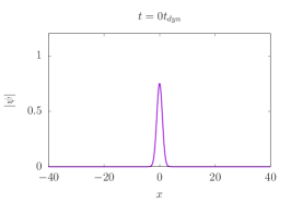
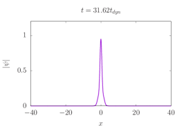
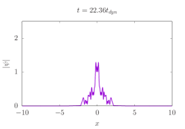
Figure 1: Snapshots of the modulus of the solution of the 1D SN equation $\left|\psi\right|$. The left plot is the initial condition, center plot and right plot correspond to the solution at the end of the simulation for $g=10$ and $g=500$ respectively.

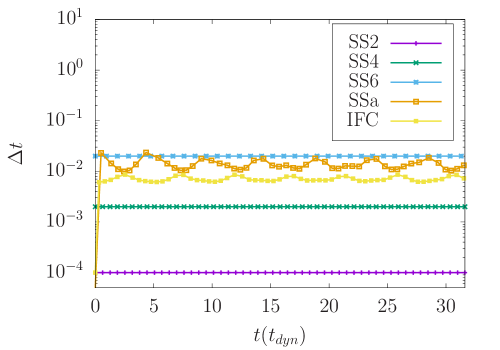
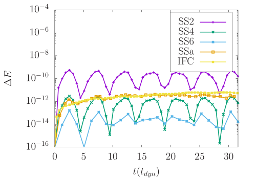
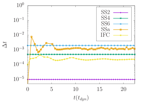
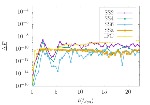
Figure 2: Comparison for the 1D SN equation between the time-step and the error on the energy conservation for the IFC method and the Split-Step solvers for both the cases $g=10$ (upper plots) and $g=500$ (lower plots).

g	Method	$\Delta t/t_{\mathrm{dyn}}$	$\overline{\Delta E}$	$\Delta\psi_{\mathrm{rev}}$	$\Delta\psi_{\mathrm{ref}}$	$T(s)$
10	SS2	$3.1\cdot 10^{-4}$	$5.5\cdot 10^{-10}$	$4.5\cdot 10^{-11}$	$4.5\cdot 10^{-9}$	123.3
	SS4	$6.3\cdot 10^{-3}$	$2.9\cdot 10^{-12}$	$2.5\cdot 10^{-12}$	$5.5\cdot 10^{-11}$	11.1
	SS6	$6.3\cdot 10^{-2}$	$1.5\cdot 10^{-13}$	$4.0\cdot 10^{-12}$	$1.1\cdot 10^{-11}$	3.5
	SSa	$4.3\cdot 10^{-2}$	$4.2\cdot 10^{-12}$	$8.5\cdot 10^{-11}$	$5.9\cdot 10^{-11}$	6.4
	IFC	2.2 $\cdot 10^{-2}$	$1.8\cdot 10^{-12}$	$1.3\cdot 10^{-10}$	$3.3\cdot 10^{-11}$	5.0
500	SS2	$10^{-5}$	$6.0\cdot 10^{-9}$	$1.1\cdot 10^{-10}$	$5.2\cdot 10^{-8}$	120.0
	SS4	$5\cdot 10^{-4}$	$2.5\cdot 10^{-9}$	$4.9\cdot 10^{-12}$	$1.3\cdot 10^{-7}$	5.4
	SS6	$2\cdot 10^{-3}$	$1.8\cdot 10^{-10}$	$2.8\cdot 10^{-11}$	$7.6\cdot 10^{-8}$	3.5
	SSa	$3.2\cdot 10^{-2}$	$1.0\cdot 10^{-10}$	$6.4\cdot 10^{-8}$	$2.9\cdot 10^{-8}$	6.7
	IFC	$5.4\cdot 10^{-3}$	$1.8\cdot 10^{-9}$	$2.3\cdot 10^{-8}$	$1.5\cdot 10^{-8}$	11.9

Table 2: Comparison for the 1D SN equation between the IFC method and the Split-Step solvers. The SSa simulations and IFC have been performed with a tolerance $\mathrm{tol}=10^{-7}$ and $\mathrm{tol}=10^{-10}$ respectively for $g=10$ and $\mathrm{tol}=10^{-6}$ and $\mathrm{tol}=10^{-10}$ respectively for $g=500$. The $\Delta t$ for adaptive algorithms is the averaged one. $T$ is the total time required to run each simulation, measured in seconds.

In table (2), we compare the Split-Step integrators with the IFC, looking at the energy conservation error, the error on the solution and the total time needed to run each simulation. Here, splitting methods proved to be faster than the integrating factor. In addition, the SS4 and SS6 performed better than the adaptive integrators. This is due the fact that, for this particular system, the extra computational cost due to the implementation of the adaptive-step is not fully compensated by the time-gain in terms of computational speed. Indeed, splitting algorithms with fixed time-step require a smaller number of computational operations to be implemented. For this reason, here, choosing a proper fixed time-step still results in a slightly faster numerical integration compared to an adaptive scheme.

3.3.1 Periodical case

We now switch to another version of the SN system, which has important applications in cosmology in order to simulate the formation of large-scale structures in the universe (4). We take $a=1$, which in cosmology corresponds to the case of a static universe [38]; we do not expect modifications of our conclusions for different cosmological models. In one dimension the equations read

$$\mathrm{i}\,\frac{\partial\,\psi}{\partial t}\ +\ \frac{1}{2}\,\frac{\partial^{2}\,\psi}{\partial x^{2}}\ -\ V\,\psi\ =\ 0,$$ (24a)

$$\frac{\partial^{2}\,V}{\partial\/x^{2}}\ =\ g\,(\left|\psi\right|^{2}-1),$$ (24b)

where the wavefunction $\left|\psi\right|^{2}$ is normalized to unity. The potential $V$ is obtained calculating the inverse of the Laplacian in Fourier space and transforming back the result to real space. We take “cold” initial conditions (see [39, 40]), namely,

$$\psi(x,t=0)\ =\ \sqrt{\rho_{0}+\delta\rho(x)}\,\exp({\mathrm{i}\theta(x)}),$$ (25)

where $\theta$ is a function whose gradient is proportional to the initial velocity field (set to zero for simplicity), $\rho_{0}$ is the background constant density and $\delta\rho(x)$ is the density fluctuations, generated as

$$\delta\rho(x)\ =\ \mathcal{F}^{-1}\left[\,R(k)\,\sqrt{P(k)}\,\right],$$ (26)

where $R(k)$ is a Gaussian random field, with zero average and unity variance. The function $P(k)$ is called Power Spectrum, and it is defined as

$$P(k)\ =\ \frac{1}{L^{d}}\,\left|\,\widehat{\delta\rho}(k)\,\right|^{2},$$ (27)

corresponding to the initial density fluctuations one wants to generate. The initial conditions are numerically initialized applying an additional filter $F(k)$ in Fourier space with the aim of setting to zero all the modes corresponding to a space scale comparable (or smaller) than the grid-step

$$F(k)\ =\ \mathrm{sech}\left(\left(k/k_{F}\right)^{10}\right),$$ (28)

with $k_{F}=k_{N}/8$, where $k_{N}$ is the Nyquist wavelength, defined as $k_{N}=\frac{N}{2L}$. Thus, the initial condition is

$$\psi(x,t=0)\ =\ \mathcal{F}^{-1}\left[\,F(k)\,\mathcal{F}\left[\sqrt{\rho_{0}+\delta\rho(x)}\right]\,\right].$$ (29)

In the simulations, space is discretized with $N=1024$ points, in a domain of length $L=1$ and a constant power spectrum is used as initial condition. We show the simulation results in the semi-classical regime. The latter corresponds to large values of the parameter $g$, as one has $g\propto\hbar^{-2}$. Specifically, we take $g=10^{6}$ (we do not observe differences in the performance in the quantum regime, i.e., for smaller values of $g$) and $\rho_{0}=1$.

In Fig. (3), the typical evolution of the system in the cosmological context is shown: the initial condition is spatially homogeneous with small fluctuations. The fluctuations grow due to gravitational interactions, up to be dominated by the finite size of the simulation box. The characteristic time of dynamics is defined as $t_{\mathrm{dyn}}=\left|g\right|^{-1/2}$.

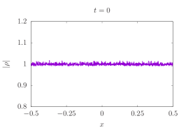
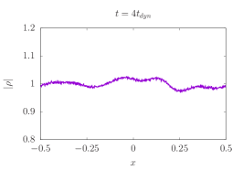
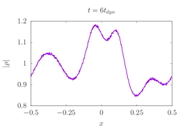
Figure 3: Snapshots of the modulus squared of the solution of the 1D SN equation (periodical case) $\left|\psi\right|^{2}$.

In Fig. 4, the Split-Step integrators are compared with the IFC. We observe for $t\gtrsim 5\/t_{\mathrm{dyn}}$ that the time-step decreases; this is due to the fact that the dynamics switches from a regime where the largest scales are still linear, to a regime where all the scales are nonlinear [15]. It indicates that the integrating factor is particularly efficient in the weakly nonlinear regime, which is the regime of interest in cosmological simulations. The Split-Step integrators (except SS2) are observed to perform in the same manner in the weakly non-linear and strongly non-linear regime. We observe that IFC outperforms the tested Split-Step integrators in the first regime, whereas, in the second one it becomes equally efficient compared to the split-step methods. This is consistent with the observation of Sect. 3.3: since the dynamics corresponds to a highly nonlinear regime, the Split-Step method performs better than the IFC one in this case. Looking to Table (3), it is clear that (for the whole simulation of this system) the IFC is the most efficient integration method.

Figure 4: Comparison for the 1D SN equation (periodical case) between the time-step (left plot) and the error on the energy conservation (right plot) for the IFC method and the Split-Step solvers.

Method	$\Delta t/t_{\mathrm{dyn}}$	$\overline{\Delta E}$	$\Delta\psi_{\mathrm{rev}}$	$\Delta\psi_{\mathrm{ref}}$	$T(s)$
SS2	$10^{-5}$	$1.6\cdot 10^{-8}$	$8.3\cdot 10^{-9}$	$8.5\cdot 10^{-10}$	276.5
SS4	$3\cdot 10^{-3}$	$1.9\cdot 10^{-8}$	$1.3\cdot 10^{-9}$	$1.5\cdot 10^{-11}$	1.8
SS6	$7\cdot 10^{-3}$	$1.1\cdot 10^{-8}$	$1.1\cdot 10^{-8}$	$3.1\cdot 10^{-11}$	2.3
SSa, $\mathrm{tol}=10^{-9}$	$5.8\cdot 10^{-3}$	$2.3\cdot 10^{-9}$	$3.3\cdot 10^{-9}$	$1.2\cdot 10^{-11}$	4.3
IFC, $\mathrm{tol}=10^{-12}$	$6.7\cdot 10^{-3}$	$1.1\cdot 10^{-8}$	$1.8\cdot 10^{-10}$	$6.7\cdot 10^{-11}$	1.3

Table 3: Comparison for the 1D SN equation (periodical case) between the IFC method and the Split-Step solvers. $T$ is the total time required to run each simulation, measured in seconds. The $\Delta t$ for adaptive algorithms is the averaged one.

3.4 2D nonlinear Schrödinger equation

In the 2D NLS case, one has

$$\mathrm{i}\,\partial_{t}\,\psi\ +\ {\textstyle{\frac{1}{2}}}\,\nabla^{2}\,\psi\ -\ g\,\left|\psi\right|^{2}\,\psi\ =\ 0.$$ (30)

The dynamics of (30) presents a finite time singularity: it can be proven [41] that there exists a finite time when the norm of the solution or of one of its derivatives becomes infinity. This happens whenever the initial condition $\psi_{0}$ satisfies $E_{g}={\textstyle{\frac{1}{2}}}\int\mathrm{d}\boldsymbol{r}\,\psi_{0}\left(g\left|\psi_{0}\right|^{2}-\nabla^{2}\right)\psi^{*}_{0}<0$. The initial condition is taken as $\psi(\boldsymbol{r},t=0)=\mathrm{e}^{-r^{2}/2}/\sqrt{\pi}$ and we study the cases $g=-1$ and $g=-6$ with respective initial energies $E_{g=-1}\approx 0.42$ and $E_{g=-6}\approx 0.02$. Thus, the latter is associated with an initial energy closer to the singular regime than the former. The simulation is run in a box of side $L=80$, discretized into $N=1024\times 1024$ points in the $g=-1$ case, while for $g=-6$ we set $L=120$ and $N=4096\times 4096$. The characteristic time of dynamics is defined as $t_{\mathrm{dyn}}=\left|g\right|^{-1/2}$.

Split-Step integrators are compared with the IFC, looking at the energy conservation error, the error on the solution and the total time needed to run each simulation. The results are illustrated in Fig. (5) and table (4).

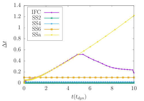
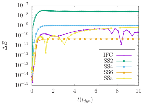
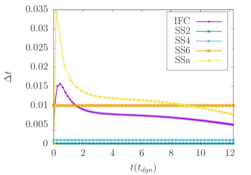
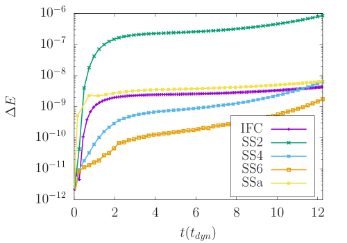
Figure 5: Comparison for the 2D NLS equation between the time-step (left panel) and the error on the energy conservation (right panel) for the IFC method and the Split-Step solvers. The top row corresponds to the $g=-1$ case while the bottom row to $g=-6$. The last time-step is chosen in such a way that the final time is the same in all simulations, in order to ensure that $\Delta\psi_{\mathrm{rev}}$ and $\Delta\psi_{\mathrm{ref}}$ are evaluated properly, which explain the step which appears for the last time point in $\Delta t$.

g	Method	$\Delta t/t_{\mathrm{dyn}}$	$\overline{\Delta E}$	$\Delta\psi_{\mathrm{rev}}$	$\Delta\psi_{\mathrm{ref}}$	$T(s)$
-1	SS2	$10^{-3}$	$3.3\cdot 10^{-8}$	$4.5\cdot 10^{-8}$	$5.0\cdot 10^{-10}$	6939
	SS4	$2\cdot 10^{-2}$	$1.1\cdot 10^{-9}$	$3.5\cdot 10^{-13}$	$7.0\cdot 10^{-11}$	830
	SS6	$10^{-1}$	$4.5\cdot 10^{-11}$	$2.5\cdot 10^{-14}$	$6.2\cdot 10^{-11}$	445
	SSa	$2.3\cdot 10^{-1}$	$7.0\cdot 10^{-10}$	$3.0\cdot 10^{-10}$	$2.5\cdot 10^{-11}$	267
	IFC	$1.7\cdot 10^{-1}$	$4.5\cdot 10^{-10}$	$3.0\cdot 10^{-10}$	$1.6\cdot 10^{-11}$	169
-6	SS2	$2.5\cdot 10^{-4}$	$8.8\cdot 10^{-7}$	$1.4\cdot 10^{-11}$	$7.9\cdot 10^{-7}$	405012
	SS4	$2.5\cdot 10^{-3}$	$6.3\cdot 10^{-9}$	$2.5\cdot 10^{-12}$	$3.7\cdot 10^{-9}$	82891
	SS6	$2.5\cdot 10^{-2}$	$1.7\cdot 10^{-9}$	$1.6\cdot 10^{-12}$	$1.8\cdot 10^{-9}$	24453
	SSa	$2.8\cdot 10^{-2}$	$6.5\cdot 10^{-9}$	$1.4\cdot 10^{-10}$	$5.4\cdot 10^{-9}$	29117
	IFC	$1.8\cdot 10^{-2}$	$2.3\cdot 10^{-9}$	$3.5\cdot 10^{-9}$	$9.4\cdot 10^{-9}$	22843

Table 4: Comparisons for the 2D NLS equation between different methods for the Dormand and Prince integrator. The $\Delta t$ for adaptive algorithms is the averaged one. $T$ is the total time required to run each simulation, measured in seconds. The tolerances of the integrator SS4(3) is $\mathrm{tol}=10^{-6}$ and $\mathrm{tol}=10^{-10}$ for the IFC.

The gain factor between splitting algorithms and the IFC method depends on the value of $g$. However, in both cases, the optimized integrating factor proved to be more efficient.

3.5 2D Schrödinger-Newton equation

In the 2D SN case, one has

$$\begin{gathered}\mathrm{i}\,\partial_{t}\,\psi\ +\ {\textstyle{\frac{1}{2}}}\,\nabla^{2}\psi\ -\ V\,\psi\ =\ 0,\qquad\nabla^{2}V\ =\ g\left|\psi\right|^{2}.\end{gathered}$$ (31)

Similarly to the one dimensional case, we use a Gaussian initial conditions $\psi(\boldsymbol{r},t=0)=\mathrm{e}^{-r^{2}/2}/\sqrt{\pi}$ and two values of the coupling constant, $g=10$ and $g=500$. The former corresponds to a system in the quantum regime and the latter is closer to the semi-classical one. The potential $V$, as in the 1D case, is calculated using the Hockney method [37]. The simulation is run in a box of side $L=40$, discretized into $N=1024^{2}$ points in the $g=10$ case, while for $g=500$ we set $L=20$ and $N=1024\times 1024$, the characteristic time of dynamics is defined as $t_{\mathrm{dyn}}=\left|g\right|^{-1/2}$.

In table (5) and Fig. (6), we compare the Split-Step and the IFC integrators, looking at the energy conservation error, the error on the solution and the total time needed to run each simulation.

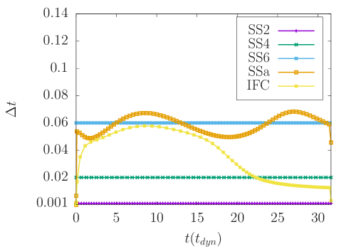
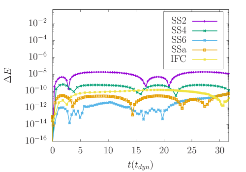
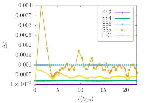
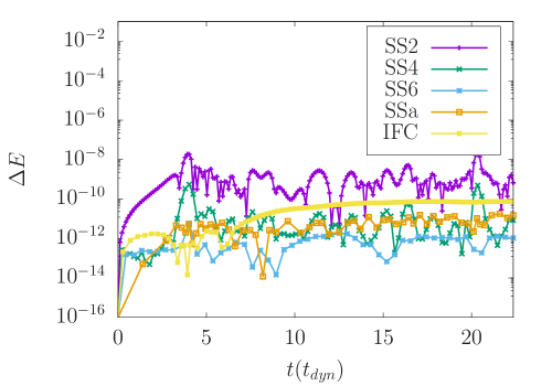
Figure 6: Comparison for the 2D SN equation between the time-step and the error on the energy conservation with the IFC method and the Split-Step solvers for both the cases $g=10$ (upper plots) and $g=500$ (lower plots).

g	Method	$\Delta t/t_{\mathrm{dyn}}$	$\overline{\Delta E}$	$\Delta\psi_{\mathrm{rev}}$	$\Delta\psi_{\mathrm{ref}}$	$T(s)$
10	SS2	$3.2\cdot 10^{-3}$	$1.8\cdot 10^{-8}$	$3.5\cdot 10^{-12}$	$1.0\cdot 10^{-7}$	9070
	SS4	$6.3\cdot 10^{-2}$	$6.0\cdot 10^{-10}$	$1.4\cdot 10^{-11}$	$3.8\cdot 10^{-8}$	959
	SS6	$1.9\cdot 10^{-1}$	$4.6\cdot 10^{-11}$	$1.6\cdot 10^{-7}$	$4.1\cdot 10^{-8}$	932
	SSa	$1.7\cdot 10^{-1}$	$4.7\cdot 10^{-11}$	$1.4\cdot 10^{-7}$	$3.9\cdot 10^{-8}$	1174
	IFC	$8.4\cdot 10^{-2}$	$1.3\cdot 10^{-10}$	$5.8\cdot 10^{-8}$	$2.9\cdot 10^{-8}$	1172
500	SS2	$2.2\cdot 10^{-4}$	$2.0\cdot 10^{-8}$	$3.1\cdot 10^{-10}$	$9.1\cdot 10^{-8}$	84030
	SS4	$4.5\cdot 10^{-3}$	$5.6\cdot 10^{-10}$	$2.8\cdot 10^{-11}$	$7.0\cdot 10^{-9}$	8401
	SS6	$2.2\cdot 10^{-2}$	$6.1\cdot 10^{-12}$	$9.1\cdot 10^{-11}$	$4.1\cdot 10^{-9}$	5143
	SSa	$2.1\cdot 10^{-2}$	$1.9\cdot 10^{-11}$	$2.0\cdot 10^{-11}$	$3.9\cdot 10^{-9}$	6676
	IFC	$9.1\cdot 10^{-3}$	$7.5\cdot 10^{-11}$	$3.0\cdot 10^{-10}$	$1.6\cdot 10^{-9}$	6637

Table 5: Comparison for the 2D SN equation between the IFC method and the Split-Step solvers. The $\Delta t$ for adaptive algorithms is the averaged one. The tolerance for the SSa algorithm is $\mathrm{tol}=10^{-6}$ and $\mathrm{tol}=10^{-7}$ for $g=10$ and $g=500$ respectively, and for the IFC algorithm $\mathrm{tol}=10^{-10}$ and $\mathrm{tol}=10^{-12}$ for $g=10$ and $g=500$ respectively.

For the 2D Schrödinger–Newton equation, adaptive splitting algorithms proved to be as efficient as the IFC. Similarly to the one-dimensional case, also here the SS6 split-step algorithm with constant time-step resulted to be the fastest among the ones we tested. This is due to the same reasons mentioned in section 3.3. Note that, here, the performance gap between the integrating factor and splitting algorithms is smaller than in the one-dimensional case. Indeed, as the dynamics gets more complicated and the number of spatial dimensions increase, algorithms with adaptive time-step shall always be preferred.

3.5.1 Periodical case

For the 2D periodical case, we run simulations in a box of side $L=1$ with $N=1024\times 1024$, using again a constant power spectrum as initial condition with $g=10^{6}$, $\rho_{0}=1$ and a zero initial velocity field. In Fig. (7) some snapshots of the modulus squared of the solution are shown, expressing time in units of $t_{\mathrm{dyn}}=1/\sqrt{g}$.

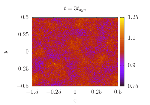
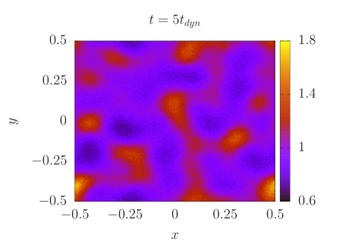
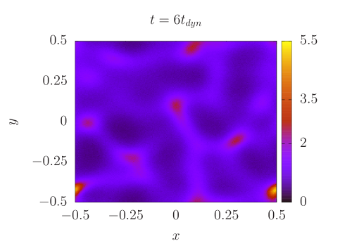
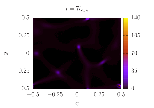
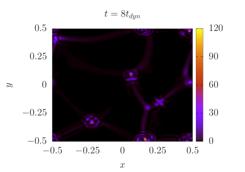
Figure 7: Snapshots of the modulus squared of the solution of the 2D SN equation (periodical case) $\left|\psi\right|^{2}$.

In table (6) and Fig. (8), we compare the Split-Step and IFC integrators, looking at the energy conservation error, the error on the solution and the total time needed to run each simulation. We obtain the same result than in one dimension, with the IFC being the most efficient method.

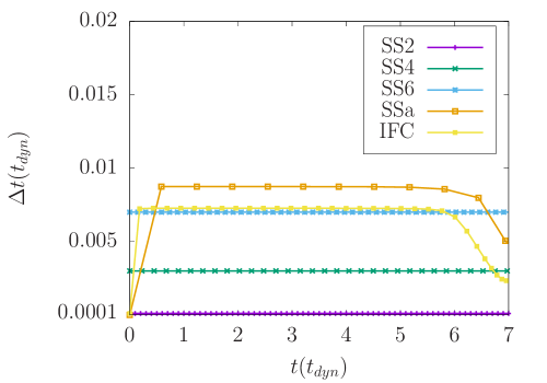
Figure 8: Comparison for the 2D SN equation (periodical case) between the time-step (left plot) and the error on the energy conservation (right plot) for the IFC method and the Split-Step solvers.

Method	$\Delta t/t_{\mathrm{dyn}}$	$\overline{\Delta E}$	$\Delta\psi_{rev}$	$\Delta\psi_{ref}$	$T(s)$
SS2	$10^{-4}$	$1.8\cdot 10^{-8}$	$4.5\cdot 10^{-9}$	$1.0\cdot 10^{-5}$	31711
SS4	$3\cdot 10^{-3}$	$4.2\cdot 10^{-8}$	$3.1\cdot 10^{-6}$	$5.3\cdot 10^{-6}$	2485
SS6	$7\cdot 10^{-3}$	$3.5\cdot 10^{-8}$	$4.5\cdot 10^{-10}$	$5.1\cdot 10^{-6}$	3046
SSa, $\mathrm{tol}=10^{-7}$	$7.5\cdot 10^{-3}$	$2.3\cdot 10^{-7}$	$8.5\cdot 10^{-7}$	$1.2\cdot 10^{-6}$	3362
IFC, $\mathrm{tol}=10^{-12}$	$5\cdot 10^{-3}$	$9.5\cdot 10^{-8}$	$4.6\cdot 10^{-6}$	$8.9\cdot 10^{-7}$	2232

Table 6: Comparison for the 2D SN equation (periodical case) between the IFC method and the Split-Step solvers. $T$ is the total time required to run each simulation, measured in seconds. The $\Delta t$ for adaptive algorithms is the averaged one.

3.6 Gross–Pitaevskii–Poisson equation

We conclude by presenting the results for the 2D Gross–Pitaevskii–Poisson equation, which is a combination of the NLS and SN equations

$$\mathrm{i}\,\partial_{t}\,\psi\ +\ {\textstyle{\frac{1}{2}}}\,\nabla^{2}\,\psi\ -V\,\psi\ =\ 0,\qquad V=V_{1}+V_{2},\qquad\nabla^{2}V_{1}\ =\ g_{1}\left|\,\psi\,\right|^{2},\qquad V_{2}\ =\ g_{2}\left|\,\psi\,\right|^{2}.$$

Based on the results presented so far, in the case of open boundary conditions, one expects the split-step or the integrating factors to outperform one the other, depending on the values of $g_{1}$ and $g_{2}$. We set them to $g_{1}=-3$ and $g_{2}=100$ which are very close to the one typically employed when simulating the collapse of a self-gravitating Bose-Einstein condensate with attractive self-interaction [21]. The numerical parameters are $N=2048\times 2048$, $L=40$ and $t_{f}=5$ while the initial condition is a Gaussian, $\psi(\boldsymbol{r},t=0)=\mathrm{e}^{-{r^{2}}/{2}}/\sqrt{\pi}$. In table 7 comparisons between the most efficient methods tested for the NLS (IFC method) and the SN in the non-periodical case (SS6 or SSa, depending on the parameters) are shown. For the values of $g_{1}$ and $g_{2}$ we use, the IFC method outperforms the split-step solvers. Moreover, we observe that for our particular initial condition, the smaller the ${g_{1}}/{g_{2}}$ ratio is, the better the IFC performs with respect to splitting methods, with a robust difference already appearing for ${g_{1}}/{g_{2}}\lessapprox 0.1$. This confirms that the presence of a short-range interaction term puts the integrating factor method in a clear more performing position, compared to splitting methods.

Method	$\Delta t$	$\overline{\Delta E}$	$\Delta\psi_{\mathrm{rev}}$	$\Delta\psi_{\mathrm{ref}}$	$T(s)$
SS6	$2.5\cdot 10^{-3}$	$1.2\cdot 10^{-9}$	$4.5\cdot 10^{-11}$	$4.5\cdot 10^{-8}$	32753
SSa, $\mathrm{tol}=10^{-7}$	$4\cdot 10^{-3}$	$2.4\cdot 10^{-11}$	$2.2\cdot 10^{-8}$	$1.4\cdot 10^{-8}$	63315
IFC, $\mathrm{tol}=10^{-11}$	$2\cdot 10^{-3}$	$7.7\cdot 10^{-10}$	$6.2\cdot 10^{-8}$	$2.3\cdot 10^{-8}$	28273

Table 7: Comparison for the 2D Gross–Pitaevskii–Poisson equation between the IFC and the Split-Step methods. $T$ is the total time required to run each simulation, measured in seconds.

4 Conclusion

We studied the numerical resolution of the nonlinear Schrödinger (NLS) and the Newton–Schrödinger (SN) equations using the optimized integrating factor (IFC) technique. This method was compared with splitting algorithms. Specifically, for the integrating factor, we tested fifth-order time-adaptive algorithms, while, for the Split-Step family, we focused on second-, fourth- and sixth-order schemes with fixed time-step, and a fourth-order algorithm with adaptive time-step. We performed extensive tests with systems in one and two spatial dimensions, with open or periodic boundary conditions.

The comparisons between the results obtained in the tested cases, show that the IFC method can be more efficient than splitting algorithms, especially in the NLS equation and periodical SN equation cases. For the SN equation in the non-periodical case on the other hand, splitting algorithms proved to be more efficient, even though the optimized integrating factor provided competitive results in terms of both speed and accuracy. Moreover, the results obtained for the Gross–Pitaevskii–Poisson equation pointed out how the presence of a short-range interaction term puts the integrating factor method in a clear more performing position.

Finally, the achieved results indicate how, among the splitting algorithms at fixed step, working with higher order solvers is always more efficient. In particular the Split-Step order 6 proved to be around 10 times faster compared with the lower order ones, while conserving the energy with the same error.

Appendix A Optimized Integrating Factor

The optimized version of the integrating factor is based on the property that, for the Schrödinger equation, if the value of the potential $V$ is modified by an additive constant $\mathcal{C}$, only the phase of the solution $\psi$ is changed. Indeed, if $\psi$ is a solution of (1) at a given time $t$, then $\Psi\stackrel{{\scriptstyle\text{\tiny{def}}}}{{=}}\psi\,\mathrm{e}^{-\/\mathrm{i}\,\mathcal{C}\,t}$ is a solution of

$$\mathrm{i}\,\partial_{t}\,\Psi\ +\ {\textstyle{\frac{1}{2}}}\,\nabla^{2}\Psi\ -\ \left(V+\mathcal{C}\right)\,\Psi\ =\ 0,$$ (33)

as it can be easily verified. Thus, adding a constant $\mathcal{C}_{n}$ to $V$, the solution is modified as

$$\psi(t_{n})\ \to\ \psi(t_{n})\,\mathrm{e}^{-\/\mathrm{i}\/\varphi},\qquad\varphi\ \stackrel{{\scriptstyle\text{\tiny{def}}}}{{=}}\ \sum_{n=0}^{N_{h}}\mathcal{C}_{n}\,h_{n},$$ (34)

where $h_{n}\stackrel{{\scriptstyle\text{\tiny{def}}}}{{=}}t_{n+1}-t_{n}$ is the $n$-th time-step and $N_{h}$ is the total number of time-steps.

The freedom provided by the gauge condition of the potential is exploited to compute an optimal value of $\mathcal{C}_{n}$, which allows to choose a larger time-step compared to the $\mathcal{C}_{n}=0$ case and therefore speeding up the numerical integration. The resulting optimal value, $\tilde{\mathcal{C}}_{n}$, which is obtained at each time step $n$ as the value of $\mathcal{C}_{n}$ minimising the $L_{2}$-norm of $\mathcal{N}$ [30], is

$$\tilde{\mathcal{C}}_{n}\,\stackrel{{\scriptstyle\text{\tiny{def}}}}{{=}}\,-\left(\,\sum_{\ell=-\left[M/2\right]}^{\left[M/2\right]-1}V_{\ell}\,\left|\psi_{\ell}\right|^{2}\,\right)\,\left/\,\left(\,\sum_{\ell=-\left[M/2\right]}^{\left[M/2\right]-1}\left|\psi_{\ell}\right|^{2}\,\right)\right.$$ (35)

where $\psi_{\ell}\stackrel{{\scriptstyle\text{\tiny{def}}}}{{=}}\psi(\boldsymbol{r}_{\ell})$ and $V_{\ell}\stackrel{{\scriptstyle\text{\tiny{def}}}}{{=}}V(\boldsymbol{r}_{\ell})$ at time $t_{n}$.

Appendix B Split-Step pseudo-codes

We list below, in ALG. (B), the pseudo-codes for the Split-Step algorithms with fixed time-step. We consider the general case of order $N$, with $N\in\left\{2,4,6\right\}$.

   1 : SSN, $N\in\left\{2,4,6\right\}$

 

1:$t\leftarrow t_{0}$

2:$\psi\leftarrow\psi(\boldsymbol{r},t_{0})$

3:while $t<t_{f}$ do

4:     $\psi\leftarrow\mathrm{FFT}^{-1}[\mathrm{exp}\left(-\mathrm{i}\hat{K}a_{1}h\right)\mathrm{FFT}[\psi]]$

5:     $\psi\leftarrow\mathrm{exp}\left(-\mathrm{i}Vb_{1}h\right)\psi$

6:     ⋮

7:     $\psi\leftarrow\mathrm{FFT}^{-1}[\mathrm{exp}\left(-\mathrm{i}\hat{K}a_{\frac{N}{2}}h\right)\mathrm{FFT}[\psi]]$

8:     $\psi\leftarrow\mathrm{exp}\left(-\mathrm{i}Vb_{\frac{N}{2}}h\right)\psi$

9:     $\psi\leftarrow\mathrm{FFT}^{-1}[\mathrm{exp}\left(-\mathrm{i}\hat{K}a_{\frac{N}{2}-1}h\right)\mathrm{FFT}[\psi]]$

10:     $\psi\leftarrow\mathrm{exp}\left(-\mathrm{i}Vb_{\frac{N}{2}-1}h\right)\psi$

11:     ⋮

12:     $\psi\leftarrow\mathrm{FFT}^{-1}[\mathrm{exp}\left(-\mathrm{i}\hat{K}a_{1}h\right)\mathrm{FFT}[\psi]]$

13:     $\psi\leftarrow\mathrm{exp}\left(-\mathrm{i}Vb_{1}h\right)\psi$

14:     $t\leftarrow t+h$

 

In the latter, $h$ is the time step, $\mathrm{FFT}$ and $\mathrm{FFT}^{-1}$ denote the Fast Fourier Transform and its inverse respectively, $\hat{K}$ is the kinetic energy operator in Fourier space, $V$ is the potential, and the values of $a_{i}$ and $b_{i}$, $i\in\left\{1,2,3,4,5,6\right\}$, are listed in table 8.

SS2	SS4	SS6
$a_{1}=\frac{1}{2}$	$a_{1}=\frac{\omega}{2}$	$a_{1}=0.0502627644003922$
$b_{1}=1$	$b_{1}=1$	$b_{1}=0.148816447901042$
	$a_{2}=\frac{1-\omega}{2}$	$a_{2}=0.413514300428344$
	$b_{2}=1-2\omega$	$b_{2}=-0.132385865767784$
		$a_{3}=0.0450798897943977$
		$b_{3}=0.067307604692185$
		$a_{4}=-0.188054853819569$
		$b_{4}=0.432666402578175$
		$a_{5}=0.541960678450780$
		$b_{5}=0.5-(b_{1}+b_{2}+b_{3}+b_{4})$
		$a_{6}=1-2(a_{1}+a_{2}+a_{3}+a_{4}+a_{5})$
		$b_{6}=1-2(a_{1}+a_{2}+a_{3}+a_{4}+a_{5})$

Table 8: Values of the parameters for the Split-Step algorithms. The quantity $\omega$ is given by $\omega=\frac{2+2^{\frac{1}{3}}+2^{-\frac{1}{3}}}{3}$.

In the case of SSa, the adaptive splitting algorithm, i.e. the SS4(3), both the solutions at the $4^{th}$ and at the $3^{rd}$ order must be evaluated. The pseudo-code is described in ALG. (B), while the coefficients are listed in 9. In our numerical tests we set $\alpha=0.9$, $\beta=3$.

   2 : SSa

 

1:$t\leftarrow t_{0}$

2:$\psi\leftarrow\psi(\boldsymbol{r},t_{0})$

3:while $t<t_{f}$ do

4:     $\psi\leftarrow\widetilde{\psi}$

5:     $\psi\leftarrow\mathrm{FFT}^{-1}[\mathrm{e}^{-\mathrm{i}\hat{K}a_{1}h}\mathrm{FFT}[\psi]]$

6:     $\psi\leftarrow\mathrm{e}^{-\mathrm{i}Vb_{1}h}\psi$

7:     ⋮

8:     $\psi\leftarrow\mathrm{FFT}^{-1}[\mathrm{e}^{-\mathrm{i}\hat{K}a_{7}h}\mathrm{FFT}[\psi]]$

9:     $\psi\leftarrow\mathrm{e}^{-\mathrm{i}Vb_{7}h}\psi$

10:     $\widetilde{\psi}\leftarrow\mathrm{FFT}^{-1}[\mathrm{e}^{-\mathrm{i}\hat{K}\overline{a}_{1}h}\mathrm{FFT}[\widetilde{\psi}]]$

11:     $\widetilde{\psi}\leftarrow\mathrm{e}^{-\mathrm{i}V\overline{b}_{1}h}\widetilde{\psi}$

12:     ⋮

13:     $\widetilde{\psi}\leftarrow\mathrm{FFT}^{-1}[\mathrm{e}^{-\mathrm{i}\hat{K}\overline{a}_{7}h}\mathrm{FFT}[\widetilde{\psi}]]$

14:     $\widetilde{\psi}\leftarrow\mathrm{e}^{-\mathrm{i}V\overline{b}_{7}h}\widetilde{\psi}$

15:     $err\leftarrow\sqrt{\frac{\sum_{i=1}^{N}\left|\psi(\boldsymbol{x}_{i},t_{n})-\widetilde{\psi}(\boldsymbol{x}_{i},t_{n})\right|^{2}}{\sum_{j=1}^{N}\left|\psi(\boldsymbol{x}_{j},t_{n})\right|^{2}}}$

16:     if $err\leq\mathrm{tol}$ then

17:         $t\leftarrow t+h$

18:     else

19:         $\psi\leftarrow\widetilde{\psi}$      

20:     $h\leftarrow h\min\left\{\alpha\left(\frac{\mathrm{tol}}{\Delta_{n}}\right)^{\frac{1}{4}},\beta\right\}$

 

SSa
Order 4		Order 3
$a_{1}$	0	$\tilde{a}_{1}$	0
$b_{1}$	0.0829844064174052	$\tilde{b}_{1}$	0.0829844064174052
$a_{2}$	0.245298957184271	$\tilde{a}_{2}$	0.245298957184271
$b_{2}$	0.3963098014983680	$\tilde{b}_{2}$	0.3963098014983680
$a_{3}$	0.604872665711080	$\tilde{a}_{3}$	0.604872665711080
$b_{3}$	-0.0390563049223486	$\tilde{b}_{3}$	-0.0390563049223486
$a_{4}$	0.5 - $(a_{2}+a_{3})$	$\tilde{a}_{4}$	0.5 - $(a_{2}+a_{3})$
$b_{4}$	1. - $2(b_{1}+b_{2}+b_{3})$	$\tilde{b}_{4}$	1. - $2(b_{1}+b_{2}+b_{3})$
$a_{5}$	0.5 - $(a_{2}+a_{3})$	$\tilde{a}_{5}$	0.3752162693236828
$b_{5}$	-0.0390563049223486	$\tilde{b}_{5}$	0.4463374354420499
$a_{6}$	0.604872665711080	$\tilde{a}_{6}$	1.4878666594737946
$b_{6}$	0.3963098014983680	$\tilde{b}_{6}$	-0.0060995324486253
$a_{7}$	0.245298957184271	$\tilde{a}_{7}$	-1.3630829287974774
$b_{7}$	0.0829844064174052	$\tilde{b}_{7}$	0

Table 9: Values of the parameters for the SSa.

References

- [1] F. Dalfovo, S. Giorgini, L. P. Pitaevskii, S. Stringari, Theory of Bose–Einstein condensation in trapped gases, Reviews of Modern Physics 71 (3) (1999) 463.
- [2] A. Hasegawa, Optical solitons in fibers, in: Optical Solitons in Fibers, Springer, 1989, pp. 1–74.
- [3] C. Kharif, E. Pelinovsky, A. Slunyaev, Rogue waves in the ocean, Springer Science & Business Media, 2008.
- [4] J. Binney, S. Tremaine, Galactic Dynamics: Second Edition, 2008.
- [5] F. Dabby, J. Whinnery, Thermal self-focusing of laser beams in lead glasses, Applied Physics Letters 13 (8) (1968) 284–286.
- [6] C. Rotschild, O. Cohen, O. Manela, M. Segev, T. Carmon, Solitons in nonlinear media with an infinite range of nonlocality: first observation of coherent elliptic solitons and of vortex-ring solitons, Physical review letters 95 (21) (2005) 213904.
- [7] C. Rotschild, B. Alfassi, O. Cohen, M. Segev, Long-range interactions between optical solitons, Nature Physics 2 (11) (2006) 769–774.
- [8] F. S. Guzman, L. A. Urena-Lopez, Gravitational cooling of self-gravitating Bose condensates, The Astrophysical Journal 645 (2) (2006) 814.
- [9] W. Hu, R. Barkana, A. Gruzinov, Fuzzy cold dark matter: the wave properties of ultralight particles, Physical Review Letters 85 (6) (2000) 1158.
- [10] A. Paredes, H. Michinel, Interference of dark matter solitons and galactic offsets, Physics of the Dark Universe 12 (2016) 50–55.
- [11] D. J. Marsh, J. C. Niemeyer, Strong constraints on fuzzy dark matter from ultrafaint dwarf galaxy Eridanus ii, Physical review letters 123 (5) (2019) 051103.
- [12] L. Diosi, Gravitation and quantumm-echanical localization of macroobjects, arXiv preprint arXiv:1412.0201 (2014).
- [13] R. Penrose, On gravity’s role in quantum state reduction, General relativity and gravitation 28 (5) (1996) 581–600.
- [14] L. M. Widrow, N. Kaiser, Using the Schrödinger equation to simulate collisionless matter, The Astrophysical Journal 416 (1993) L71.
- [15] P. J. E. Peebles, The large-scale structure of the universe, 1980.
- [16] N. Banik, A. J. Christopherson, P. Sikivie, E. M. Todarello, Linear Newtonian perturbation theory from the Schrödinger–Poisson equations, Phys.Rev. D 91 (12) (2015) 123540. doi:10.1103/PhysRevD.91.123540.
- [17] C. Conti, M. Peccianti, G. Assanto, Route to nonlocality and observation of accessible solitons, Physical review letters 91 (7) (2003) 073901.
- [18] Y. Izdebskaya, W. Krolikowski, N. F. Smyth, G. Assanto, Vortex stabilization by means of spatial solitons in nonlocal media, Journal of Optics 18 (5) (2016) 054006.
- [19] D. O’dell, S. Giovanazzi, G. Kurizki, V. Akulin, Bose–Einstein condensates with interatomic attraction: Electromagnetically induced “gravity”, Physical Review Letters 84 (25) (2000) 5687.
- [20] A. Suárez, P.-H. Chavanis, Cosmological evolution of a complex scalar field with repulsive or attractive self-interaction, Physical Review D 95 (6) (2017) 063515.
- [21] P.-H. Chavanis, Collapse of a self-gravitating Bose–Einstein condensate with attractive self-interaction, Physical Review D 94 (8) (2016) 083007.
- [22] A. Bernal, F. S. Guzman, Scalar field dark matter: Head-on interaction between two structures, Physical Review D 74 (10) (2006) 103002.
- [23] P. Bader, S. Blanes, F. Casas, M. Thalhammer, Efficient time integration methods for Gross–Pitaevskii equations with rotation term, arXiv preprint arXiv:1910.12097 (2019).
- [24] C. Besse, G. Dujardin, I. Lacroix-Violet, High order exponential integrators for nonlinear Schrödinger equations with application to rotating Bose–Einstein condensates, SIAM J. Numer. Anal. 55 (3) (2017) 1387–1411.
- [25] J. R. Dormand, P. J. Prince, A family of embedded Runge–Kutta formulae, J. Comp. Appl. Math. 6 (1) (1980) 19–26.
- [26] C. Tsitouras, Runge–Kutta pairs of order satisfying only the first column simplifying assumption, Computers & Mathematics with Applications 62 (2) (2011) 770–775.
- [27] R. Alexander, Solving ordinary differential equations i: Nonstiff problems (e. hairer, sp norsett, and g. wanner), Siam Review 32 (3) (1990) 485.
- [28] C. Canuto, M. Y. Hussaini, A. Quarteroni, T. A. Zang, Spectral Methods. Fundamentals in Single Domains, 2nd Edition, Scientific Computation, Springer, 2008.
- [29] J. C. Butcher, Numerical methods for ordinary differential equations, John Wiley & Sons, 2016.
- [30] M. Lovisetto, D. Clamond, B. Marcos, Optimized integrating factor technique for schrödinger-like equations, Applied Numerical Mathematics 178 (2022) 329–336.
- [31] S. Blanes, F. Casas, A. Murua, Splitting and composition methods in the numerical integration of differential equations, arXiv preprint arXiv:0812.0377 (2008).
- [32] M. Suzuki, General theory of fractal path integrals with applications to many-body theories and statistical physics, Journal of Mathematical Physics 32 (2) (1991) 400–407.
- [33] H. Holden, K. H. Karlsen, K.-A. Lie, Splitting methods for partial differential equations with rough solutions: Analysis and MATLAB programs, Vol. 11, European Mathematical Society, 2010.
- [34] M. Thalhammer, J. Abhau, A numerical study of adaptive space and time discretisations for Gross–Pitaevskii equations, Journal of computational physics 231 (20) (2012) 6665–6681.
- [35] S. Blanes, P. C. Moan, Practical symplectic partitioned Runge–Kutta and Runge–Kutta–Nyström methods, Journal of Computational and Applied Mathematics 142 (2) (2002) 313–330.
- [36] M. Thalhammer, High-order exponential operator splitting methods for time-dependent Schrödinger equations, SIAM Journal on Numerical Analysis 46 (4) (2008) 2022–2038.
- [37] R. W. Hockney, J. W. Eastwood, Computer simulation using particles, crc Press, 2021.
- [38] S. Weinberg, Cosmology, OUP Oxford, 2008.
-
[39]
G. Davies, L. M. Widrow, Test-bed
simulations of collisionless, self-gravitating systems using the
Schrödinger method, The Astrophysical Journal 485 (2) (1997) 484–495.
doi:10.1086/304440.
URL https://doi.org/10.1086/304440 -
[40]
P. Mocz, L. Lancaster, A. Fialkov, F. Becerra, P.-H. Chavanis,
Schrödinger–Poisson
Vlasov–Poisson correspondence, Phys. Rev. D 97 (2018) 083519.
doi:10.1103/PhysRevD.97.083519.
URL https://link.aps.org/doi/10.1103/PhysRevD.97.083519 - [41] C. Sulem, P.-L. Sulem, The nonlinear Schrödinger equation: self-focusing and wave collapse, Vol. 139, Springer Science & Business Media, 2007.