Electric double layers with modulated surface charge density: Exact 2D results

Abstract

Electric double layers (EDL) with counterions only, say electrons with the elementary charge $-e$, in thermal equilibrium at the inverse temperature $\beta$ are considered. In particular, we study the effect of the surface charge modulation on the particle number density profile and the pressure. The mobile particles are constrained to the surface of a 2D cylinder and immersed in vacuum (no dielectric image charges). An EDL corresponds to the end-circle of the cylinder which carries a (fixed) position-dependent line charge density. The geometries of one single EDL and two EDLs at distance $d$ are considered; the particle density profile is studied for both geometries, the effective interaction of two EDLs is given by the particle pressure on either of the line walls. For any coupling constant $\Gamma\equiv\beta e^{2}=2\times{\rm integer}$, there exists a mapping of the 2D one-component Coulomb system onto the 1D interacting anticommuting-field theory defined on a chain of sites. Using specific transformation symmetries of anticommuting variables, the contact value theorem is generalized to the EDL with modulated line charge density. For the free-fermion coupling $\Gamma=2$ it is shown that, under certain conditions, the matrix of interaction strengths between anticommuting variables diagonalizes itself which permits one to obtain exact formulas for the particle density profile as well as the pressure. The obtained results confirm the previous indications of weak-coupling and Monte Carlo observations that the surface charge inhomogeneity implies an enhancement of the counterion density at the contact with the charged line and a diminution of the pressure between two parallel lines in comparison with the uniformly charged ones (with the same mean charge densities).

Keywords: Electric double layer, modulated surface charge density, contact value theorem, exactly solvable 2D Coulomb models

1 Introduction

Equilibrium statistical mechanics of classical particle systems interacting pairwisely via the Coulomb potential is of particular interest in soft matter and condensed matter physics. In Gauss units, the three-dimensional (3D) Coulomb potential in vacuum (dielectric constant $\varepsilon=1$) has the form $\phi({\bf r})=1/r$ where $r$ is the modulus of ${\bf r}$. The definition of the Coulomb potential can be extended to any Euclidean space of dimension $\nu=1,2,\ldots$ as the solution of the Poisson equation

$$\Delta\phi({\bf r})=-s_{\nu}\delta({\bf r}),$$ (1.1)

where $s_{\nu}=2\pi^{\nu/2}/\Gamma(\nu/2)$ is the surface area of the $\nu$-dimensional unit sphere. The Fourier component of $\phi({\bf r})$ exhibits the singular behaviour of type $1/k^{2}$ which preserves many generic properties of 3D Coulomb systems like screening and the corresponding sum rules [1]. In an infinite two-dimensional (2D) space, the solution of (1.1), subject to the boundary condition $\nabla\phi({\bf r})\to 0$ as $r\to\infty$, reads as $-\ln(r/L)$ where $L$ is a free length scale. The system of 2D pointlike charges can be represented in the real 3D space as parallel infinite charged lines perpendicular to the given surface, the model which mimics 3D polyelectrolytes. In one dimension (1D), the Coulomb potential is given by $-r$.

In this paper, we study one-component Coulomb models of mobile pointlike particles of the same (say elementary) charge $-e$. In contrast to the standard jellium systems, the neutralizing background charge density is spread over boundary surfaces of the domain the charged particles are confined to. This kind of models occurs in biological experiments with colloids immersed in polar solvents like the water. The colloid surface acquires a surface charge density by releasing micro-ions into the polar solvent [2, 3]. The fixed surface charge density is opposite to the charge of mobile particles which are therefore referred to as “counterions”. In theoretical studies, the curved surface of large colloids is usually substituted by a flat surface and the modulated charge density on the colloid’s surface by the uniform one.

In the one-wall geometry, the charged surface and the surrounding counterions in thermal equilibrium form a neutral entity known as the electric double layer (EDL) [4, 5, 6, 7]. The particle number density at the flat surface is related to the wall’s uniform surface charge density via a simple contact-value theorem [8, 9, 10, 11]. As concerns the geometry of two parallel uniformly charged walls with counterions in between, their effective interaction mediated by counterions is of particular interest [12]. To obtain the effective interaction of the walls, one calculates the pressure from counterion densities at the contact with either of the walls. A counter-intuitive attraction of like-charged colloids was observed at small enough temperatures, experimentally [13, 14, 15, 16, 17] as well as by computer simulations [4, 18, 19]; for more recent progress in the field, see reviews [20, 21].

The weak-coupling (WC) limit of models with uniformly charged surfaces and counterions only is described by the mean-field Poisson-Boltzmann (PB) theory [2] and its systematic improvement via a loop expansion [5, 22, 23]. The strong-coupling (SC) limit is more controversial. Based on a virial fugacity expansion, the leading SC term of the particle number density corresponds to a single-particle theory in the electric potential induced by charged wall(s) [24, 25, 26] which was confirmed by Monte Carlo (MC) simulations [24, 25, 27, 28]. Next correction orders of the virial SC approach fail to reproduce correctly MC data. Another type of SC theories is based on the creation of classical Wigner crystals on the wall surfaces at zero temperature [29, 30, 31]. A harmonic expansion of the interaction energy in particle deviations from their ground-state Wigner positions [32, 33] reproduces the leading single-particle theory and implies a first correction term to the counterion density which is also in excellent agreement with MC data, from strong up to intermediate Coulombic couplings. The accuracy of the analytic results was improved by adapting the idea of a correlation hole [34, 35] into the Wigner-structure description in [36, 37].

The subject of interest in this paper is the effect of the space modulation of the fixed surface charge density on plates on the density profile of counterions and the effective interaction between two plates. The discreteness of the surface charge is omnipresent in real systems and often plays a dominant role in bio-interfacial phenomena [38, 39]. Numerous experimental studies are reviewed in [40]. Early theoretical approaches were based on liquid-state theory [41, 42]. Analytic perturbation techniques were combined with MC simulations to describe the effect of surface charge inhomogeneities in the WC [43, 44] and SC [45] regimes. The obtained results indicate an enhancement of the counterion density close the charge-modulated surface in comparison with the uniformly charged one (with the same mean charge density). As concerns the geometry of two parallel inhomogeneously charged surfaces, according to the PB theory the increase of the counterion density close to surfaces means a decrease of counterions at the midplane and, consequently, a diminution of the pressure [46, 47]. Exact PB solutions of one planar or cylindrical EDL with the surface charge modulation along one direction only were found recently by exploring in an inverse way the general solution of the 2D Liouville equation [48].

As concerns the thermal equilibrium of 2D plasmas, the relevant parameter is the coupling constant $\Gamma=\beta e^{2}/\varepsilon$ with $\beta=1/(k_{\rm B}T)$ being the inverse temperature and $\varepsilon$ (set to unity, for simplicity) the dielectric constant of the medium the particles are immersed in. 2D Coulomb systems are of special interest because besides the PB limit $\Gamma\to 0$ their thermodynamics and many-body densities are exactly solvable also at the finite (free-fermion) coupling $\Gamma=2$, in the bulk [49, 50] and in the semi-infinite as well as fully finite geometries [51, 52]. Another advantage of the 2D one-component systems is an explicit representation of their partition function and particle densities for the sequence of the coupling constants $\Gamma=2\gamma$ where $\gamma$ is a positive integer (in the fluid regime), expressing the integer powers of Vandermonde determinant by using either Jack polynomials [53, 54] or anticommuting-field theory defined on a one-dimensional (1D) chain of sites [55, 56, 57, 58]. In the case of uniform surface charge densities with counterions only at $\Gamma=2$, the density profile of counterions for the one-wall geometry was derived in [59, 60] and the effective interaction between two parallel asymmetrically charged plates at distance $d$ in [61].

The aim of this work is to extend, within the anticommuting-field representation, exact results for 2D one-component plasmas with uniformly charged plates to plates with periodically modulated surface charge densities. Using a cylinder geometry of the confining domain and applying certain linear transformations of anticommuting variables leading to specific sum rules, the contact value theorem for uniformly charged lines is generalized to the lines with periodically modulated surface charge densities at arbitrary coupling constant $\Gamma$. Under certain conditions, the periodic modulation of the surface charge density does not destroy the exact solvability of the 2D counterions systems at $\Gamma=2$. Our exact results confirm previous WC and MC observations about the effect of surface charge inhomogeneities on the enhancement of the density of counterions at the wall contact and the diminution of the pressure between two plates.

The paper is organized as follows. In section 2, we present the general formalism of the canonical ensemble for the system of identical charges confined to the surface of a cylinder, for both cases of a single EDL (section 2.1) and two parallel EDLs (section 2.2) with the modulated line charge densities. Section 3 concerns general results obtained from the mapping of the 2D one-component Coulomb system onto the anticommuting-field theory on a 1D chain of sites. The mapping for the coupling $\Gamma=2\gamma$ ($\gamma$ a positive integer) is reviewed in section 3.1, section 3.2 deals with the exactly solvable free-fermion case $\Gamma=2$ and section 3.3 is devoted to the derivation of sum rules for correlators of anticommuting variables. Exact results for the geometry of one EDL are reported in section 4. The previously derived sum rules are used to generalize the contact value theorem for uniformly charged lines to inhomogeneously charged lines in section 4.1. Special conditions under which the model is exactly solvable at the free-fermion coupling $\Gamma=2$ are shown in section 4.2. Exact results for the geometry of two parallel EDLs are reported in section 5. A counterpart of the contact value theorem is derived in section 5.1, a general formula for the pressure in terms of the counterion density profile valid for any coupling constant $\Gamma$ is given in section 5.2. As concerns the free-fermion coupling constant $\Gamma=2$, the counterion density profile is derived in section 5.3 and the pressure in section 5.4. A short recapitulation is outlined in the concluding section 6.

2 Cylinder geometry

Let $N$ mobile pointlike particles with the elementary charge $-e$ be confined to the surface of a cylinder of circumference $W$. The surface of the cylinder is equivalent to a 2D rectangle domain $\Lambda$ of points ${\bf r}=(x,y)$ with coordinates $y\in[0,W]$ and the periodic boundary conditions at $y=0,W$. The dielectric constant of the medium the particles are immersed in is equal to that of vacuum, $\varepsilon=1$, and there are no dielectric image charges.

The Coulomb potential $\phi$ at a spatial position ${\bf r}\in\Lambda$, induced by a unit charge at the origin ${\bf 0}$, is defined as the solution of the 2D Poisson equation (1.1) under the periodicity requirement along the $y$-axis with period $W$. Writing the potential as a discrete Fourier series in $y$, it reads as [62]

$$\phi({\bf r})=\frac{1}{W}\sum_{k_{y}}\int_{-\infty}^{\infty}{\rm d}k_{x}\frac{1}{k_{x}^{2}+k_{y}^{2}}{\rm e}^{{\rm i}(k_{x}x+k_{y}y)},\qquad k_{y}\in\frac{2\pi n}{W}$$ (2.1)

with $n=0,\pm 1,\ldots$ being any integer. In the mixed continuous-discrete $(k_{x},k_{y})$ Fourier space, the Coulomb potential has the typical $1/k^{2}$ $(k^{2}=k_{x}^{2}+k_{y}^{2})$ singularity as $k\to 0$. Integrating over the continuous variable $k_{x}$ and summing over the discrete variable $k_{y}$, one obtains

$$\phi(x,y) = -\ln\left|2\sinh\left(\frac{\pi z}{W}\right)\right|$$ (2.2)

$$= -\frac{1}{2}\ln\left[2\cosh\left(\frac{2\pi x}{W}\right)-2\cos\left(\frac{2\pi y}{W}\right)\right]$$

with the complex number notation $z=x+{\rm i}y$ and $\bar{z}=x-{\rm i}y$. For small distances $r\ll W$, this potential takes the expected 2D logarithmic form $-\ln(2\pi r/W)$. At large distances along the cylinder axis $x\gg W$, this potential is the 1D Coulomb one $-\pi|x|/W$.

In what follows, the following integral for the periodic Coulomb potential (2.2)

$$\int_{0}^{W}{\rm d}y\,\phi({\bf r})=-\frac{W}{4\pi}\int_{0}^{2\pi}{\rm d}y\,\ln\left[2\cosh\left(\frac{2\pi x}{W}\right)-2\cos y\right]$$ (2.3)

will be important. Writing

$$2\cosh\left(\frac{2\pi x}{W}\right)=a+\frac{1}{a},\qquad a=\exp\left(\frac{2\pi x}{W}\right)\geq 1$$ (2.4)

and using that

$$\int_{0}^{2\pi}{\rm d}y\,\ln\left(1+a^{2}-2a\cos y\right)=4\pi\ln a,\qquad a\geq 1,$$ (2.5)

one obtains that the integral

$$\int_{0}^{W}{\rm d}y\,\phi({\bf r})=-\pi x$$ (2.6)

does not depend on the length $W$. The important feature of this formula is the absence of an infinite constant which occurs in the analogous integral over the pure 2D Coulomb potential $-\frac{1}{2}\int_{-\infty}^{\infty}{\rm d}y\,\ln(x^{2}+y^{2})$.

2.1 Single EDL

In the one-wall geometry of figure 1, there is an inhomogeneous line charge density $\sigma(y)e$ ($y\in[0,W]$) fixed at $x=0$; $\sigma(y)$ has the dimension of inverse length. Being motivated by experiments with colloids, the sign of the line charge density is supposed to be the same everywhere,

$$\sigma(y)\geq 0,\qquad y\in[0,W].$$ (2.7)

The particles of the elementary charge $-e$ move in the semi-infinite space $\Lambda=\{(x,y);x>0,y\in[0,W]\}$.

The condition of the overall system electroneutrality reads as

$$N=\int_{0}^{W}{\rm d}y\,\sigma(y).$$ (2.8)

Under the effect of the inhomogeneous line charge density, the one-body energy of the particle at position $(x,y)$ is given by

$$v(x,y)=-e^{2}\int_{0}^{W}{\rm d}y^{\prime}\,\sigma(y^{\prime})\phi(x,y-y^{\prime}).$$ (2.9)

Introducing the mean value of the line charge density

$$\sigma\equiv\frac{1}{W}\int_{0}^{W}{\rm d}y\,\sigma(y)=\frac{N}{W}$$ (2.10)

and its deviation from the mean value

$$\delta\sigma(y)\equiv\sigma(y)-\sigma,\qquad\int_{0}^{W}{\rm d}y\,\delta\sigma(y)=0,$$ (2.11)

using the integration formula (2.6) one can write the one-body energy (2.9) as follows

$$v(x,y)=\pi e^{2}\sigma x-e^{2}\int_{0}^{W}{\rm d}y^{\prime}\,\delta\sigma(y^{\prime})\phi(x,y-y^{\prime}).$$ (2.12)

Figure 1: The cylinder geometry with the periodic boundary conditions (period $W$) along the $y$-axis. The line (circle) at $x=0$ is charged by the line density $\sigma(y)e$. Pointlike counterions of charge $-e$, represented by black circles, move freely in the semi-infinite domain $\Lambda=\{(x,y);x>0,y\in[0,W]\}$.

The Coulomb energy of $N$ particles at spatial positions $\{{\bf r}_{1},\ldots,{\bf r}_{N}\}$ inside the domain $\Lambda$ plus the line charge density at $x=0$ consists of three parts, $E_{N}=E_{ll}+E_{lp}+E_{pp}$, where

$$E_{ll} = \frac{e^{2}}{2}\int_{0}^{W}{\rm d}y\int_{0}^{W}{\rm d}y^{\prime}\sigma(y)\phi(0,y-y^{\prime})\sigma(y^{\prime})$$ (2.13)

$$= \frac{e^{2}}{2}\int_{0}^{W}{\rm d}y\int_{0}^{W}{\rm d}y^{\prime}\delta\sigma(y)\phi(0,y-y^{\prime})\delta\sigma(y^{\prime})$$

is the self-energy of the line charge density at $x=0$,

$$E_{lp}=\sum_{j=1}^{N}v(x_{j},y_{j})$$ (2.14)

describes the interaction of the line charge density with the particles and

$$E_{pp}=e^{2}\sum_{(j<k)=1}^{N}\phi({\bf r}_{j}-{\bf r}_{k})=-e^{2}\sum_{(j<k)=1}^{N}\left|2\sinh\left(\frac{\pi(z_{j}-z_{k})}{W}\right)\right|$$ (2.15)

is the sum over all pair interactions among the particles.

The Boltzmann factor of the total energy at the inverse temperature $\beta$ is given by

$${\rm e}^{-\beta E_{N}(\{{\bf r}\})} = {\rm e}^{-\frac{\Gamma}{2}\int_{0}^{W}{\rm d}y\int_{0}^{W}{\rm d}y^{\prime}\delta\sigma(y)\phi(0,y-y^{\prime})\delta\sigma(y^{\prime})}\prod_{j=1}^{N}{\rm e}^{-\beta v(x_{j},y_{j})}$$ (2.16)

$$\times\prod_{(j<k)=1}^{N}\left|2\sinh\frac{\pi(z_{j}-z_{k})}{W}\right|^{\Gamma},$$

where $\Gamma\equiv\beta e^{2}$ is the coupling constant. Within the framework of the canonical ensemble, the partition function is defined as

$$Z_{N}=\frac{1}{N!}\int_{\Lambda}\frac{{\rm d}{\bf r}_{1}}{\lambda^{2}}\cdots\int_{\Lambda}\frac{{\rm d}{\bf r}_{N}}{\lambda^{2}}{\rm e}^{-\beta E_{N}(\{{\bf r}\})},$$ (2.17)

where $\lambda$ is the thermal de Broglie wavelength. Applying the formula

$$\left|2\sinh\frac{\pi(z-z^{\prime})}{W}\right|={\rm e}^{\frac{\pi}{W}(x+x^{\prime})}\left|{\rm e}^{-\frac{2\pi}{W}z}-{\rm e}^{-\frac{2\pi}{W}z^{\prime}}\right|$$ (2.18)

for each two-body Boltzmann factor, the partition function (2.17) is expressible as

$$Z_{N}=\left(\frac{W^{2}}{4\pi\lambda^{2}}\right)^{N}{\rm e}^{-\frac{\Gamma}{2}\int_{0}^{W}{\rm d}y\int_{0}^{W}{\rm d}y^{\prime}\,\delta\sigma(y)\phi(0,y-y^{\prime})\delta\sigma(y^{\prime})}Q_{N},$$ (2.19)

where

$$Q_{N}=\frac{1}{N!}\int_{\Lambda}\prod_{j=1}^{N}\left[{\rm d}^{2}z_{j}\,w({\bf r}_{j})\right]\prod_{(j<k)=1}^{N}\left|{\rm e}^{-\frac{2\pi}{W}z_{j}}-{\rm e}^{-\frac{2\pi}{W}z_{k}}\right|^{\Gamma}$$ (2.20)

with the renormalized one-body weight function

$$w({\bf r})=\frac{4\pi}{W^{2}}\exp\left[-\beta v(x,y)+\frac{\pi\Gamma}{W}(N-1)x\right].$$ (2.21)

With regard to the equality (2.12), one has

$$w({\bf r})=\frac{4\pi}{W^{2}}\exp\left[-\frac{\pi\Gamma}{W}x+\Gamma\int_{0}^{W}{\rm d}y^{\prime}\,\delta\sigma(y^{\prime})\phi(x,y-y^{\prime})\right].$$ (2.22)

The free energy $F_{N}$ is defined by $-\beta F_{N}=\ln Z_{N}$. With respect to (2.19), it is expressible as

$$-\beta F_{N}(\gamma) = N\ln\left(\frac{W^{2}}{4\pi\lambda^{2}}\right)-\frac{\Gamma}{2}\int_{0}^{W}{\rm d}y\int_{0}^{W}{\rm d}y^{\prime}\,\delta\sigma(y)\phi(0,y-y^{\prime})\delta\sigma(y^{\prime})$$ (2.23)

$$+\ln Q_{N}(\gamma).$$

Introducing the microscopic particle number density $\hat{n}({\bf r})=\sum_{j=1}^{N}\delta({\bf r}-{\bf r}_{j})$, the mean particle number density at point ${\bf r}\in\Lambda$ is given by

$$n({\bf r})=\left\langle\hat{n}({\bf r})\right\rangle,\qquad$$ (2.24)

where $\langle\cdots\rangle$ denotes the statistical average over the canonical ensemble. Since in the partition function (2.19) only the multiple integral $Q_{N}$ involves particle coordinates, the particle density can be obtained as the functional derivative

$$n({\bf r})=w({\bf r})\frac{1}{Q_{N}}\frac{\delta Q_{N}}{\delta w({\bf r})}.$$ (2.25)

Since there is a finite number of particles per unit length of the line wall, the particle number density must vanish at large distances from the wall,

$$\lim_{x\to\infty}n(x,y)=0.$$ (2.26)

2.2 Two parallel EDLs

In the case of two parallel walls at distance $d$ (see figure 2), there are “left” and “right” line charge densities $\sigma_{L}(y)e$ and $\sigma_{R}(y)e$ fixed on the line segments at the end-points $x=0$ and $x=d$, respectively, such that

$$\sigma_{L}(y)\geq 0,\quad\sigma_{R}(y)\geq 0,\qquad y\in[0,W].$$ (2.27)

The mobile charges are constrained to the space between the walls $\Lambda=\{(x,y);0<x<d,y\in[0,W]\}$. The electroneutrality condition reads as

$$N=\int_{0}^{W}{\rm d}y\,\left[\sigma_{L}(y)+\sigma_{R}(y)\right].$$ (2.28)

The mean values of the left and right line charge densities

$$\sigma_{L}\equiv\frac{1}{W}\int_{0}^{W}{\rm d}y\,\sigma_{L}(y),\qquad\sigma_{R}\equiv\frac{1}{W}\int_{0}^{W}{\rm d}y\,\sigma_{R}(y)$$ (2.29)

are constrained by

$$\sigma_{L}+\sigma_{R}=\frac{N}{W}.$$ (2.30)

The deviations of the left and right line charge densities from their mean values are defined by

$$\delta\sigma_{L}(y)\equiv\sigma_{L}(y)-\sigma_{L},\qquad\int_{0}^{W}{\rm d}y\,\delta\sigma_{L}(y)=0$$ (2.31)

and

$$\delta\sigma_{R}(y)\equiv\sigma_{R}(y)-\sigma_{R},\qquad\int_{0}^{W}{\rm d}y\,\delta\sigma_{R}(y)=0,$$ (2.32)

respectively. The one-body energy of the particle at position $(x,y)$ reads as

$$v(x,y) = -e^{2}\int_{0}^{W}{\rm d}y^{\prime}\,\sigma_{L}(y^{\prime})\phi(x,y-y^{\prime})$$ (2.33)

$$-e^{2}\int_{0}^{W}{\rm d}y^{\prime}\,\sigma_{R}(y^{\prime})\phi(d-x,y-y^{\prime}).$$

Using (2.6), it can be written as

$$v(x,y) = \pi e^{2}\sigma_{R}d+\pi e^{2}\left(\sigma_{L}-\sigma_{R}\right)x-e^{2}\int_{0}^{W}{\rm d}y^{\prime}\,\delta\sigma_{L}(y^{\prime})\phi(x,y-y^{\prime})$$ (2.34)

$$-e^{2}\int_{0}^{W}{\rm d}y^{\prime}\,\delta\sigma_{R}(y^{\prime})\phi(d-x,y-y^{\prime}).$$

Figure 2: The cylinder geometry with the periodic boundary conditions (period $W$) along the $y$-axis. Two parallel lines (circles) with the fixed charge densities $\sigma_{L}(y)e$ and $\sigma_{R}(y)e$ are localized at the left and right end points $x=0$ and $x=d$, respectively. Pointlike counterions of charge $-e$ (black circles) move freely between the two charged lines.

The total Coulomb energy of $N$ particles at spatial positions $\{{\bf r}_{1},\ldots,{\bf r}_{N}\}$ inside the domain $\Lambda$ plus the left and right line charge densities at $x=0$ and $x=d$, respectively, consists of three parts: $E_{N}=E_{ll}+E_{lp}+E_{pp}$. The self-energies and the interaction energy of the line charge densities at $x=0$ and $x=d$ are given by

$$E_{ll} = \frac{e^{2}}{2}\int_{0}^{W}{\rm d}y\int_{0}^{W}{\rm d}y^{\prime}\sigma_{L}(y)\phi(0,y-y^{\prime})\sigma_{L}(y^{\prime})$$ (2.35)

$$+\frac{e^{2}}{2}\int_{0}^{W}{\rm d}y\int_{0}^{W}{\rm d}y^{\prime}\sigma_{R}(y)\phi(0,y-y^{\prime})\sigma_{R}(y^{\prime})$$

$$+e^{2}\int_{0}^{W}{\rm d}y\int_{0}^{W}{\rm d}y^{\prime}\sigma_{L}(y)\phi(d,y-y^{\prime})\sigma_{R}(y^{\prime})$$

$$= \frac{e^{2}}{2}\int_{0}^{W}{\rm d}y\int_{0}^{W}{\rm d}y^{\prime}\delta\sigma_{L}(y)\phi(0,y-y^{\prime})\delta\sigma_{L}(y^{\prime})$$

$$+\frac{e^{2}}{2}\int_{0}^{W}{\rm d}y\int_{0}^{W}{\rm d}y^{\prime}\delta\sigma_{R}(y)\phi(0,y-y^{\prime})\delta\sigma_{R}(y^{\prime})$$

$$+e^{2}\int_{0}^{W}{\rm d}y\int_{0}^{W}{\rm d}y^{\prime}\delta\sigma_{L}(y)\phi(d,y-y^{\prime})\delta\sigma_{R}(y^{\prime})$$

$$-\pi e^{2}\sigma_{L}\sigma_{R}Wd.$$

The interaction energy of the line charge densities with the particles $E_{lp}$ is given by formula (2.14) with the one-body potential $v(x,y)$ substituted from (2.34). The formula (2.15) for the particle-particle interaction $E_{pp}$ remains unchanged.

Repeating the procedure in the paragraph between equations (2.16) and (2.23) accomplished for the one-wall case, the (dimensionless) free energy takes the form

$$-\beta F_{N} = N\ln\left(\frac{W^{2}}{4\pi\lambda^{2}}\right)-\frac{\Gamma}{2}\int_{0}^{W}{\rm d}y\int_{0}^{W}{\rm d}y^{\prime}\,\delta\sigma_{L}(y)\phi(0,y-y^{\prime})\delta\sigma_{L}(y^{\prime})$$ (2.36)

$$-\frac{\Gamma}{2}\int_{0}^{W}{\rm d}y\int_{0}^{W}{\rm d}y^{\prime}\,\delta\sigma_{R}(y)\phi(0,y-y^{\prime})\delta\sigma_{R}(y^{\prime})$$

$$-\Gamma\int_{0}^{W}{\rm d}y\int_{0}^{W}{\rm d}y^{\prime}\,\delta\sigma_{L}(y)\phi(d,y-y^{\prime})\delta\sigma_{R}(y^{\prime})$$

$$-\pi\Gamma\sigma_{R}^{2}Wd+\ln Q_{N},$$

where $Q_{N}$ is defined by (2.20) with the renormalized one-body weight function (2.21) of the form

$$w(x,y) = \frac{4\pi}{W^{2}}\exp\Bigg{\{}-\frac{\pi\Gamma}{W}x+2\pi\Gamma\sigma_{R}x+\Gamma\int_{0}^{W}{\rm d}y^{\prime}\,\delta\sigma_{L}(y^{\prime})\phi(x,y-y^{\prime})$$ (2.37)

$$+\Gamma\int_{0}^{W}{\rm d}y^{\prime}\,\delta\sigma_{R}(y^{\prime})\phi(d-x,y-y^{\prime})\Bigg{\}}.$$

The pressure $P_{N}$, i.e. the force between the left and right charged line fragments (per unit length of one of the lines), is given by

$$\beta P_{N} = \frac{\partial}{\partial d}\left(\frac{-\beta F_{N}}{W}\right)$$ (2.38)

$$= -\frac{\Gamma}{W}\int_{0}^{W}{\rm d}y\int_{0}^{W}{\rm d}y^{\prime}\,\delta\sigma_{L}(y)\frac{\partial\phi(d,y-y^{\prime})}{\partial d}\delta\sigma_{R}(y^{\prime})$$

$$-\pi\Gamma\sigma_{R}^{2}+\frac{1}{WQ_{N}}\frac{\partial Q_{N}}{\partial d}.$$

The calculation of the one-body density by using the generating functional $Q_{N}$ proceeds as in the one-wall case, see equation (2.25).

3 Formalism of anticommuting variables

3.1 Mapping onto the 1D lattice anticommuting-field theory

For $\Gamma=2\gamma$ ($\gamma=1,2,3,\ldots$ a positive integer), the generating functional $Q_{N}$ (2.20) can be expressed as an integral over Grassmann (anticommuting) variables [55, 56]; for the cylinder geometry the mapping is established in [57, 63].

Let us consider a discrete chain of $N$ sites $j=0,1,\ldots,N-1$. At each site $j$, there is $\gamma$ variables of type $\{\xi_{j}^{(\alpha)}\}$ and $\gamma$ variables of type $\{\psi_{j}^{(\alpha)}\}$ $(\alpha=1,\ldots,\gamma)$, the variables anticommute with each other. The multi-dimensional integral of the form (2.20) is expressible as the integral over anticommuting variables as follows

$$Q_{N}=\int{\cal D}\psi{\cal D}\xi\,{\rm e}^{S(\Xi,\Psi)},\qquad S(\Xi,\Psi)=\sum_{j,k=0}^{\gamma(N-1)}\Xi_{j}w_{jk}\Psi_{k}.$$ (3.1)

Here, ${\cal D}\psi{\cal D}\xi\equiv\prod_{j=0}^{N-1}{\rm d}\psi_{j}^{(\gamma)}\cdots{\rm d}\psi_{j}^{(1)}{\rm d}\xi_{j}^{(\gamma)}\cdots{\rm d}\xi_{j}^{(1)}$ and the action $S(\Xi,\Psi)$ involves pair interactions of composite operators

$$\Xi_{j}=\sum_{j_{1},\ldots,j_{\gamma}=0\atop(j_{1}+\cdots+j_{\gamma}=j)}^{N-1}\xi_{j_{1}}^{(1)}\cdots\xi_{j_{\gamma}}^{(\gamma)},\qquad\Psi_{j}=\sum_{j_{1},\ldots,j_{\gamma}=0\atop(j_{1}+\cdots+j_{\gamma}=j)}^{N-1}\psi_{j_{1}}^{(1)}\cdots\psi_{j_{\gamma}}^{(\gamma)},$$ (3.2)

i.e. the products of $\gamma$ anticommuting variables of one type with the prescribed sum of site indices. The interaction strengths $w_{jk}$ $[j,k=0,1,\ldots,\gamma(N-1)]$ are given by

$$w_{jk}=\int_{\Lambda}{\rm d}^{2}z\,w(z,\bar{z})\exp\left(-\frac{2\pi}{W}jz\right)\exp\left(-\frac{2\pi}{W}k\bar{z}\right).$$ (3.3)

The particle number density at the point ${\bf r}=(z,\bar{z})$ is given by

$$n({\bf r})=w({\bf r})\sum_{j,k=0}^{\gamma(N-1)}\langle\Xi_{j}\Psi_{k}\rangle\exp\left(-\frac{2\pi}{W}jz\right)\exp\left(-\frac{2\pi}{W}k\bar{z}\right),$$ (3.4)

where

$$\langle\cdots\rangle\equiv\frac{1}{Q_{N}}\int{\cal D}\psi{\cal D}\xi\,{\rm e}^{S(\Xi,\Psi)}\cdots.$$ (3.5)

denotes the average over the anticommuting variables.

3.2 Exactly solvable coupling $\Gamma=2$

The formalism simplifies itself for the coupling $\Gamma=2$ ($\gamma=1$) when the composite operators $\{\Xi_{j},\Psi_{j}\}_{j=0}^{N-1}$ become the standard anticommuting variables $\{\xi_{j},\psi_{j}\}_{j=0}^{N-1}$. Due to the bilinear form of the action $S=\sum_{j,k=0}^{N-1}\xi_{j}w_{jk}\psi_{k}$, it holds that

$$Q_{N} = {\rm Det}(w_{jk})|_{j,k=0}^{N-1},$$ (3.6)

$$\langle\xi_{j}\psi_{k}\rangle = w^{-1}_{kj}.$$ (3.7)

The $N\times N$ matrix $w_{jk}$ can be inverted only in specific cases. The most trivial case is the diagonal form of the matrix $w_{jk}=w_{j}\delta_{jk}$ $(j,k=0,1,\ldots,N-1)$ when

$$Q_{N}=\prod_{j=0}^{N-1}w_{j},\qquad w^{-1}_{kj}=w^{-1}_{jk}=\frac{1}{w_{j}}\delta_{jk}.$$ (3.8)

Thus, the particle number density is given by

$$n(x,y)=w(x,y)\sum_{j=0}^{N-1}\frac{1}{w_{j}}\exp\left(-\frac{4\pi}{W}jx\right).$$ (3.9)

3.3 Sum rules

There exist linear transformations of anticommuting variables $\{\xi\}$ or $\{\psi\}$ which maintain the composite form of the operators $\{\Xi\}$ or $\{\Psi\}$ [64]. Every transformation implies exact constraints (sum rules) for the correlators $\langle\Xi_{j}\Psi_{k}\rangle$ and, consequently, integral equations for one-body densities. Here, we make use of two simplest transformations.

$\bullet$ Let at each site one of the field components, say $\{\xi^{(1)}\}$, be rescaled by a constant $\mu$:

$$\xi_{j}^{(1)}\to\mu\xi_{j}^{(1)},\qquad j=0,1,\ldots,N-1.$$ (3.10)

The Jacobian of this transformation equals to $\mu^{N}$. The composite operators $\{\Xi\}$ get the same factor $\mu$ and the action in (3.1) is transformed as follows $S(\Xi,\Psi)\to\mu S(\Xi,\Psi)$. Consequently,

$$Q_{N}=\mu^{-N}\int{\cal D}\psi{\cal D}\xi\exp\left(\mu\sum_{j,k=0}^{\gamma(N-1)}\Xi_{j}w_{jk}\Psi_{k}\right).$$ (3.11)

Since $Q_{N}$ is independent of $\mu$, its derivative with respect to $\mu$ is zero for any value of $\mu$. Choosing $\mu=1$, the equality $\partial\ln Q_{N}/\partial\mu|_{\mu=1}=0$ is equivalent to

$$\sum_{j,k=0}^{\gamma(N-1)}w_{jk}\langle\Xi_{j}\Psi_{k}\rangle=N.$$ (3.12)

Using the definition of the interaction strength $w_{jk}$ (3.3) and the representation (3.4) of $n(z,\bar{z})$, this relation is equivalent to the trivial information

$$\int_{\Lambda}{\rm d}^{2}z\,n(z,\bar{z})=N$$ (3.13)

that there are just $N$ particles in the cylinder domain $\Lambda$.

$\bullet$ Let us rescale at each site all anticommuting field $\xi$-components as follows

$$\xi_{j}^{(\alpha)}\to\lambda^{j}\xi_{j}^{(\alpha)},\qquad\alpha=1,\ldots,\gamma,\qquad j=0,1,\ldots,N-1,$$ (3.14)

or all anticommuting field $\psi$-components,

$$\psi_{j}^{(\alpha)}\to\lambda^{j}\psi_{j}^{(\alpha)},\qquad\alpha=1,\ldots,\gamma,\qquad j=0,1,\ldots,N-1.$$ (3.15)

The Jacobian of both transformations equals to $\lambda^{\gamma N(N-1)/2}$. Under the transformation (3.14), the composite operators $\Xi_{j}$ acquire the factor $\lambda^{j}$ and the action in (3.1) transforms itself to $S(\Xi,\Psi)\to\sum_{j,k=0}^{\gamma(N-1)}\lambda^{j}\Xi_{j}w_{jk}\Psi_{k}$. Thus,

$$Q_{N}=\lambda^{-\gamma N(N-1)/2}\int{\cal D}\psi{\cal D}\xi\exp\left(\sum_{j,k=0}^{\gamma(N-1)}\lambda^{j}\Xi_{j}w_{jk}\Psi_{k}\right).$$ (3.16)

Analogously, under the transformation (3.15), the composite operators $\Psi_{j}$ acquire the factor $\lambda^{j}$ and the action in (3.1) transforms itself to $S(\Xi,\Psi)\to\sum_{j,k=0}^{\gamma(N-1)}\lambda^{k}\Xi_{j}w_{jk}\Psi_{k}$, i.e.,

$$Q_{N}=\lambda^{-\gamma N(N-1)/2}\int{\cal D}\psi{\cal D}\xi\exp\left(\sum_{j,k=0}^{\gamma(N-1)}\lambda^{k}\Xi_{j}w_{jk}\Psi_{k}\right).$$ (3.17)

The requirement $\partial\ln Q_{N}/\partial\lambda|_{\lambda=1}=0$ is equivalent to the sum rules

$$\sum_{j,k=0}^{\gamma(N-1)}jw_{jk}\langle\Xi_{j}\Psi_{k}\rangle = \frac{1}{2}\gamma N(N-1),$$ (3.18)

$$\sum_{j,k=0}^{\gamma(N-1)}kw_{jk}\langle\Xi_{j}\Psi_{k}\rangle = \frac{1}{2}\gamma N(N-1).$$ (3.19)

These equalities can be rewritten into a more suitable form

$$\sum_{j,k=0}^{\gamma(N-1)}(j+k)w_{jk}\langle\Xi_{j}\Psi_{k}\rangle = \gamma N(N-1),$$ (3.20)

$$\sum_{j,k=0}^{\gamma(N-1)}(j-k)w_{jk}\langle\Xi_{j}\Psi_{k}\rangle = 0.$$ (3.21)

4 Analytic results for one EDL

4.1 Derivation of the contact value theorem

With regard to the definition of the interaction strengths (3.3), the first sum rule (3.20) can be expressed as

$$\int_{\Lambda}{\rm d}^{2}z\,w(z,\bar{z})\sum_{j,k=0}^{\gamma(N-1)}(j+k)\langle\Xi_{j}\Psi_{k}\rangle\exp\left[-\frac{2\pi}{W}(j+k)x-\frac{2\pi}{W}(j-k){\rm i}y\right]$$

$$=\gamma N(N-1).$$ (4.1)

Using the expression for the particle density (3.4), this equation is expressed as

$$-\frac{W}{2\pi}\int_{\Lambda}{\rm d}^{2}z\,w(z,\bar{z})\frac{\partial}{\partial x}\left[\frac{n(z,\bar{z})}{w(z,\bar{z})}\right]=\frac{\Gamma}{2}N(N-1).$$ (4.2)

Thus,

$$-\int_{\Lambda}{\rm d}^{2}r\,\frac{\partial}{\partial x}n(x,y)+\int_{\Lambda}{\rm d}^{2}r\,n(x,y)\frac{\partial}{\partial x}\left[\ln w(x,y)\right] = \frac{\pi\Gamma}{W}N(N-1).$$

For the geometry of one wall with the one-body weight function $w(x,y)$ (2.22), it holds that

$$\frac{\partial}{\partial x}\ln w(x,y)=-\frac{\pi\Gamma}{W}+\Gamma\int_{0}^{W}{\rm d}y^{\prime}\,\delta\sigma(y^{\prime})\frac{\partial\phi(x,y-y^{\prime})}{\partial x}.$$ (4.4)

Taking into account the boundary condition (2.26) and the equality (2.10), one finally gets the contact value theorem

$$\int_{0}^{W}{\rm d}y\,\left[n(0,y)-\pi\Gamma\sigma^{2}\right]+\Gamma\int_{0}^{W}{\rm d}y\int_{0}^{\infty}{\rm d}x\,n(x,y)$$

$$\times\int_{0}^{W}{\rm d}y^{\prime}\,\delta\sigma(y^{\prime})\frac{\partial\phi(x,y-y^{\prime})}{\partial x}=0.$$ (4.5)

Although the outlined derivation was performed only for the discrete series of the coupling constants $\Gamma/2=$integer, it is reasonable to anticipate its validity also for continuous values of $\Gamma$.

In the case of a homogeneously charged line with $\delta\sigma(y)=0$, this relation reduces itself to the standard 2D contact value theorem relating the contact density $n(0,y)=n(0)$ to the uniform line charge density $\sigma$ as follows

$$n(0)=\Gamma\pi\sigma^{2}.$$ (4.6)

Note that in the presence of the line charge modulation the contact density $n(0,y)$, integrated over the domain boundary, depends on the density profile $n(x,y)$ inside the whole region $\Lambda$.

The second sum rule (3.21) is equivalent to the condition

$$\int_{\Lambda}{\rm d}^{2}z\,w(z,\bar{z})\frac{\partial}{\partial y}\left[\frac{n(z,\bar{z})}{w(z,\bar{z})}\right]=0.$$ (4.7)

Taking into account the continuity and periodicity of the density along the $y$-axis, $n(x,W)=n(x,0)$, this condition is equivalent to the one

$$\int_{0}^{W}{\rm d}y\int_{0}^{\infty}{\rm d}x\,n(x,y)\int_{0}^{W}{\rm d}y^{\prime}\,\delta\sigma(y^{\prime})\frac{\partial\phi(x,y-y^{\prime})}{\partial y}=0.$$ (4.8)

4.2 The exactly solvable coupling $\Gamma=2$

For the free-fermion coupling $\Gamma=2$, the renormalized one-body weight function (2.22) takes the form

$$w(x,y)=\frac{4\pi}{W^{2}}\exp\left[-\frac{2\pi}{W}x+2\int_{0}^{W}{\rm d}y^{\prime}\,\delta\sigma(y^{\prime})\phi(x,y-y^{\prime})\right].$$ (4.9)

We assume that the deviation of the line charge density from its mean value is a continuous and periodic function of the $y$-coordinate,

$$\delta\sigma(y)=\delta\sigma(y+\lambda),\qquad\lambda=\frac{W}{M}\quad(M=1,2,\ldots).$$ (4.10)

Note that the condition for $M$ being a positive integer ensures the continuity of $\delta\sigma(y)$ across the cylinder boundary along the $y$-axis, $\delta\sigma(y)=\delta\sigma(y+W)$. The periodicity of $\delta\sigma(y)$ automatically means the periodicity of the one-body weight function (4.9),

$$w(x,y)=w(x,y+\lambda).$$ (4.11)

Within the anticommuting-field representation, the interaction strengths (3.3) are given by

$$w_{jk} = \int_{0}^{\infty}{\rm d}x\,{\rm e}^{-\frac{2\pi}{W}(j+k)x}U(j-k,x),$$

$$U(\alpha,x) = \int_{0}^{W}{\rm d}y\,w(x,y){\rm e}^{-{\rm i}\frac{2\pi}{W}\alpha y}.$$ (4.12)

In the diagonal case $j=k$, the integral

$$U(0,x)=M\int_{0}^{\lambda}{\rm d}y\,w(x,y)>0$$ (4.13)

and so the diagonal elements

$$w_{jj}\equiv w_{j}=\int_{0}^{\infty}{\rm d}x\,{\rm e}^{-\frac{4\pi}{W}jx}U(0,x)$$ (4.14)

are positive numbers. For the off-diagonal $j\neq k$ elements, the integral $U(\alpha,x)$ with $\alpha=\pm 1,\pm 2,\ldots,\pm(N-1)$ can be expressed as

$$U(\alpha,x)=\int_{0}^{\lambda}{\rm d}y\,w(x,y){\rm e}^{-{\rm i}\frac{2\pi}{W}\alpha y}\left(1+q+q^{2}+\cdots+q^{M-1}\right),$$ (4.15)

where $q=\exp\left(-{\rm i}\frac{2\pi}{W}\alpha\lambda\right)=\exp\left(-{\rm i}\frac{2\pi}{M}\alpha\right)$. To ensure that $q\neq 1$, let us assume that $M\geq N$ or, with regard to the equalities $M=W/\lambda$ and $N=\sigma W$,

$$\lambda\sigma\leq 1.$$ (4.16)

Note that the equality $\lambda\sigma=1$ corresponds to the most interesting case when there is just one counterion per the surface-charge period (i.e. there is one electron released by one “blurred” nucleus at the wall). The summation of the finite geometric series in (4.15) then results in

$$\frac{q^{M}-1}{q-1}=\frac{{\rm e}^{-{\rm i}2\pi\alpha}-1}{q-1}=0.$$ (4.17)

This means that the matrix of interaction strengths is diagonal, $w_{jk}=w_{j}\delta_{jk}$, with the positive diagonal elements

$$w_{j}=\frac{W}{\lambda}\int_{0}^{\infty}{\rm d}x\,\exp\left(-\frac{4\pi}{W}jx\right)\int_{0}^{\lambda}{\rm d}y\,w(x,y),$$ (4.18)

$j=0,1,\ldots,N-1$. The particle number density is given by the relation (3.9). In the case of the opposite inequality $M<N$, the $N\times N$ matrix of interaction strengths $w_{jk}$ is no longer diagonal and as such cannot be inverted analytically; the model is thus not explicitly solvable.

The previous analysis was general, valid for any function $\delta\sigma(y)$ satisfying the periodicity condition (4.10). For simplicity, let us now restrict ourselves on the periodic cosine dependence

$$\delta\sigma(y)=A\cos\left(\frac{2\pi}{\lambda}y\right).$$ (4.19)

This form of the surface charge modulation describes adequately real solid electrodes consisting of a periodic array of positively charged heavy nuclei, bound together with core electrons and vibrating thermally around their local equilibrium positions, and delocalized (in the case of conductors) light valence electrons. To ensure the physical requirement (2.7), the real amplitude $A$ with dimension of inverse length must obey the inequality

$$|A|\leq\sigma.$$ (4.20)

The integral term in the exponential of the definition of $w(x,y)$ (4.9)

$$V(x,y)=2\int_{0}^{W}{\rm d}y^{\prime}\,\delta\sigma(y^{\prime})\phi(x,y-y^{\prime})$$ (4.21)

can be expressed as

$$V(x,y) = -A\int_{0}^{W}{\rm d}y^{\prime}\,\cos\left(\frac{2\pi}{\lambda}y^{\prime}\right)\ln\left\{1+a^{2}-2a\cos\left[\frac{2\pi}{W}(y-y^{\prime})\right]\right\},$$

where the parameter $a=\exp\left(2\pi x/W\right)\geq 1$ has already been introduced in (2.4). Using the substitution $t=2\pi(y^{\prime}-y)/W$ in the integral (LABEL:int1) implies

$$V(x,y)=-A\frac{W}{2\pi}\int_{0}^{2\pi}{\rm d}t\,\cos\left(\frac{2\pi}{\lambda}y+Mt\right)\ln\left(1+a^{2}-2a\cos t\right).$$ (4.23)

Writing $\cos\left(\frac{2\pi}{\lambda}y+Mt\right)=\cos\left(\frac{2\pi}{\lambda}y\right)\cos(Mt)-\sin\left(\frac{2\pi}{\lambda}y\right)\sin(Mt)$ and using the equalities

$$\int_{0}^{2\pi}{\rm d}t\,\sin(Mt)\ln\left(1+a^{2}-2a\cos t\right) = 0,$$ (4.24)

$$\int_{0}^{2\pi}{\rm d}t\,\cos(Mt)\ln\left(1+a^{2}-2a\cos t\right) = -\frac{2\pi}{M}a^{-M}$$ (4.25)

valid for $M=1,2,\ldots$ and $a>1$, one obtains that

$$V(x,y)=\lambda A\exp\left(-\frac{2\pi}{\lambda}x\right)\cos\left(\frac{2\pi}{\lambda}y\right).$$ (4.26)

Finally, since

$$w(x,y)=\frac{4\pi}{W^{2}}\exp\left[-\frac{2\pi}{W}x+\lambda A{\rm e}^{-\frac{2\pi}{\lambda}x}\cos\left(\frac{2\pi}{\lambda}y\right)\right],$$ (4.27)

the diagonal elements (4.18) take the form

$$w_{j}=\frac{4\pi}{W}\int_{0}^{\infty}{\rm d}x\,{\rm e}^{-\frac{4\pi}{W}(j+\frac{1}{2})x}I_{0}\left(\lambda A{\rm e}^{-\frac{2\pi}{\lambda}x}\right),$$ (4.28)

where

$$I_{0}(t)=\frac{1}{\pi}\int_{0}^{\pi}{\rm d}\varphi\,{\rm e}^{t\cos\varphi}$$ (4.29)

is the Bessel function of the first kind with imaginary argument [65].

According to the formula (3.9), the particle number density is yielded by

$$n(x,y)=\frac{4\pi}{W^{2}}\exp\left[\lambda A{\rm e}^{-\frac{2\pi}{\lambda}x}\cos\left(\frac{2\pi}{\lambda}y\right)\right]\sum_{j=0}^{N-1}\frac{1}{w_{j}}\exp^{-\frac{4\pi}{W}\left(j+\frac{1}{2}\right)x}.$$ (4.30)

The sum over $j$ simplifies itself in the thermodynamic limit $N,W\to\infty$, with the fixed ratio $N/W=\sigma$; in this limit, the wall corresponds to an infinite line and charges interact via the pure 2D logarithmic Coulomb potential. Introducing the continuous variable $t=\frac{1}{N}\left(j+\frac{1}{2}\right)$ and transforming the sum $\frac{1}{N}\sum_{j=0}^{N-1}$ to the integral $\int_{0}^{1}{\rm d}t$, one arrives at

$$n(x,y) = \frac{N}{W}\exp\left[\lambda A{\rm e}^{-\frac{2\pi}{\lambda}x}\cos\left(\frac{2\pi}{\lambda}y\right)\right]$$ (4.31)

$$\times\int_{0}^{1}{\rm d}t\,\frac{{\rm e}^{-4\pi\sigma tx}}{\int_{0}^{\infty}{\rm d}x^{\prime}\,{\rm e}^{-4\pi\sigma tx^{\prime}}I_{0}\left(\lambda A{\rm e}^{-\frac{2\pi}{\lambda}x^{\prime}}\right)}.$$

Finally, with the aid of the substitution $s=4\pi\sigma t$, one gets

$$n(x,y) = \frac{1}{4\pi}\exp\left[\lambda A{\rm e}^{-\frac{2\pi}{\lambda}x}\cos\left(\frac{2\pi}{\lambda}y\right)\right]$$ (4.32)

$$\times\int_{0}^{4\pi\sigma}{\rm d}s\,\frac{{\rm e}^{-sx}}{\int_{0}^{\infty}{\rm d}x^{\prime}\,{\rm e}^{-sx^{\prime}}I_{0}\left(\lambda A{\rm e}^{-\frac{2\pi}{\lambda}x^{\prime}}\right)}.$$

This particle number density is periodic along the $y$-axis, with the same period $\lambda$ as the line charge density. It must obey, within the interval of one period, the electroneutrality condition

$$\frac{1}{\lambda}\int_{0}^{\infty}{\rm d}x\int_{0}^{\lambda}{\rm d}y\,n(x,y)=\sigma.$$ (4.33)

It is easy to check that our result (4.32) indeed satisfies this constraint.

Based on the proven equivalence of equations (4.21) and (4.26), it holds that

$$\frac{\partial}{\partial x}\int_{0}^{W}{\rm d}y^{\prime}\,\delta\sigma(y^{\prime})\phi(x,y-y^{\prime})=-\pi A\exp\left(-\frac{2\pi}{\lambda}x\right)\cos\left(\frac{2\pi}{\lambda}y\right).$$ (4.34)

Considering this equation in the contact value theorem (4.5) taken at $\Gamma=2$ and reducing the integration interval over $y\in[0,W]$ to a series of equivalent integrals over one period $\lambda$, one obtains a simplified form of the contact value theorem

$$\int_{0}^{\lambda}{\rm d}y\,\left[n(0,y)-2\pi\sigma^{2}\right]=2\pi A\int_{0}^{\lambda}{\rm d}y\int_{0}^{\infty}{\rm d}x\,n(x,y){\rm e}^{-\frac{2\pi}{\lambda}x}\cos\left(\frac{2\pi}{\lambda}y\right).$$

(4.35)

Inserting here the result for the counterion density (4.32) and using that

$$-2\pi A{\rm e}^{-\frac{2\pi}{\lambda}x}\cos\left(\frac{2\pi}{\lambda}y\right)\exp\left[\lambda A{\rm e}^{-\frac{2\pi}{\lambda}x}\cos\left(\frac{2\pi}{\lambda}y\right)\right]$$

$$=\frac{\partial}{\partial x}\exp\left[\lambda A{\rm e}^{-\frac{2\pi}{\lambda}x}\cos\left(\frac{2\pi}{\lambda}y\right)\right],$$ (4.36)

the subsequent integration by parts together with the definition of the Bessel function (4.29) confirm the validity of the contact value theorem (4.35).

In the case of the uniform line charge density $(A=0)$, taking into account that $I_{0}(0)=1$, the formula (4.32) implies the particle number density which depends only on the $x$-coordinate:

$$n(x) = \frac{1}{4\pi}\int_{0}^{4\pi\sigma}{\rm d}s\,s{\rm e}^{-xs}$$ (4.37)

$$= \frac{1}{4\pi x^{2}}\left[1-\left(1+4\pi\sigma x\right){\rm e}^{-4\pi\sigma x}\right],\qquad A=0,$$

see also [59, 60, 61]. The counterion density at the contact with the charged line $n(0)=2\pi\sigma^{2}$ is in agreement with the contact value theorem (4.6) taken at the coupling constant $\Gamma=2$.

The result (4.32) tells us that the particle number density at the charged line ($x=0$) reads as

$$n(0,y) = \frac{1}{4\pi}\exp\left[\lambda A\cos\left(\frac{2\pi}{\lambda}y\right)\right]\int_{0}^{4\pi\sigma}{\rm d}s\,\frac{1}{\int_{0}^{\infty}{\rm d}x^{\prime}\,{\rm e}^{-sx^{\prime}}I_{0}\left(\lambda A{\rm e}^{-\frac{2\pi}{\lambda}x^{\prime}}\right)}.$$

The mean value of the contact counterion density along the $y$-axis is given by

$$\bar{n}(0)=\frac{1}{\lambda}\int_{0}^{\lambda}{\rm d}y\,n(0,y)=\frac{1}{4\pi}\int_{0}^{4\pi\sigma}{\rm d}s\,\frac{I_{0}(\lambda A)}{\int_{0}^{\infty}{\rm d}x^{\prime}\,{\rm e}^{-sx^{\prime}}I_{0}\left(\lambda A{\rm e}^{-\frac{2\pi}{\lambda}x^{\prime}}\right)}.$$ (4.39)

Provided that $\lambda\neq 0$, using the substitutions $x^{\prime}=\lambda x^{\prime\prime}$ and $s=r/\lambda$ this relation can be rewritten in a dimensionless form

$$\lambda^{2}\bar{n}(0)=\frac{1}{4\pi}\int_{0}^{4\pi\lambda\sigma}{\rm d}r\,\frac{I_{0}(\lambda A)}{\int_{0}^{\infty}{\rm d}x^{\prime\prime}\,{\rm e}^{-rx^{\prime\prime}}I_{0}\left(\lambda A{\rm e}^{-2\pi x^{\prime\prime}}\right)}.$$ (4.40)

Here, the dimensionless quantity $\lambda^{2}\bar{n}(0)$ is the function of the dimensionless variables $\lambda\sigma$ and $\lambda A$; the condition (4.16) restricts $\lambda\sigma\leq 1$ and the condition (4.20) restricts $|\lambda A|\leq\lambda\sigma$. Since the Bessel function $I_{0}(t)$ grows with increasing the argument $t$, it holds that $I_{0}(\lambda A)\geq I_{0}\left(\lambda A{\rm e}^{-2\pi x^{\prime\prime}}\right)$ for $0\leq x^{\prime\prime}\leq\infty$. Consequently,

$$\bar{n}(0)\geq 2\pi\sigma^{2}$$ (4.41)

where the equality takes place for the homogeneous line charge density $(A=0)$ only. We conclude that the variation of the line charge density around its mean value $\sigma e$ induces an enhancement of the counterion density at the wall in comparison with the line charged uniformly by $\sigma e$, irrespective of the amplitude $A$ and the period $\lambda$ of the cosine modulation. This result, obtained in 2D at the finite coupling constant $\Gamma=2$, is in agreement with the mean-field predictions and MC simulations [43, 44, 45].

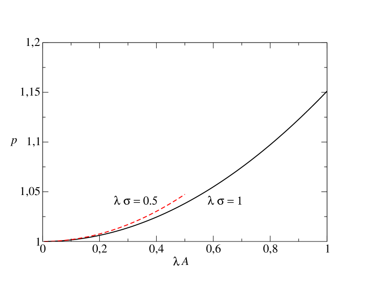
Figure 3: The plots of the ratio (4.42) ($p\geq 1$) versus the dimensionless amplitude $\lambda A$ of the cosine modification of the uniform line charge density $\sigma$. The solid curve corresponds to $\lambda\sigma=1$ $(\lambda A\in[0,1])$ and the dashed curve to $\lambda\sigma=0.5$ $(\lambda A\in[0,0.5])$.

The numerical plots of the ratio

$$p(\lambda\sigma,\lambda A)=\frac{\bar{n}(0)}{2\pi\sigma^{2}}=\frac{1}{8(\pi\lambda\sigma)^{2}}\int_{0}^{4\pi\lambda\sigma}{\rm d}r\,\frac{I_{0}(\lambda A)}{\int_{0}^{\infty}{\rm d}x^{\prime\prime}\,{\rm e}^{-rx^{\prime\prime}}I_{0}\left(\lambda A{\rm e}^{-2\pi x^{\prime\prime}}\right)}$$ (4.42)

versus the dimensionless amplitude $\lambda A$ of the cosine modification (4.19) of the uniform line charge density $\sigma$ are pictured in figure 3 for two values of the dimensionless $\lambda\sigma$. The solid curve corresponds to $\lambda\sigma=1$ $(\lambda A\in[0,1])$ and the dashed curve to $\lambda\sigma=0.5$ $(\lambda A\in[0,0.5])$. It is seen that the ratio $p$ is always greater than 1 as it should be. For a fixed value of $\lambda A$, the ratio $p$ increases with decreasing $\lambda\sigma$.

5 Effective interaction between two parallel EDLs

5.1 Analogue of the contact value theorem

For the geometry of two parallel walls at distance $d$, one can proceed as in the single wall case up to equation (LABEL:crucialeq). Inserting there the equality

$$\frac{\partial}{\partial x}\ln w(x,y) = -\frac{\pi\Gamma}{W}+2\pi\Gamma\sigma_{R}+\Gamma\int_{0}^{W}{\rm d}y^{\prime}\,\delta\sigma_{L}(y^{\prime})\frac{\partial\phi(x,y-y^{\prime})}{\partial x}$$ (5.1)

$$+\int_{0}^{W}{\rm d}y^{\prime}\,\delta\sigma_{R}(y^{\prime})\frac{\partial\phi(d-x,y-y^{\prime})}{\partial x}$$

holding for the one-body weight function $w(x,y)$ (2.37), one gets

$$\frac{W}{2\pi}\int_{0}^{W}{\rm d}y\,\left[n(0,y)-n(d,y)\right]+W\Gamma\sigma_{R}N+\frac{W\Gamma}{2\pi}\int_{0}^{W}{\rm d}y\int_{0}^{\infty}{\rm d}x\,n(x,y)$$

$$\times\int_{0}^{W}{\rm d}y^{\prime}\,\left[\delta\sigma_{L}(y^{\prime})\frac{\partial\phi(x,y-y^{\prime})}{\partial x}+\delta\sigma_{R}(y^{\prime})\frac{\partial\phi(d-x,y-y^{\prime})}{\partial x}\right]=\frac{\Gamma}{2}N^{2}.$$

Using the electroneutrality condition (2.30), this relation can be expressed as

$$\int_{0}^{W}{\rm d}y\,\left[n(0,y)-\pi\Gamma\sigma_{L}^{2}\right]$$

$$+\Gamma\int_{0}^{W}{\rm d}y\int_{0}^{d}{\rm d}x\,n(x,y)\int_{0}^{W}{\rm d}y^{\prime}\,\delta\sigma_{L}(y^{\prime})\frac{\partial\phi(x,y-y^{\prime})}{\partial x}$$

$$=\int_{0}^{W}{\rm d}y\,\left[n(d,y)-\pi\Gamma\sigma_{R}^{2}\right]$$

$$-\Gamma\int_{0}^{W}{\rm d}y\int_{0}^{d}{\rm d}x\,n(x,y)\int_{0}^{W}{\rm d}y^{\prime}\,\delta\sigma_{R}(y^{\prime})\frac{\partial\phi(d-x,y-y^{\prime})}{\partial x}.$$ (5.3)

This equation defines specific combinations of integrals over the particle and line charge densities which are invariant with respect the left or right EDLs. Note that in the limit $d\to\infty$, when the two EDLs decouple from one another, both sides of equation (5.3) vanish due to the contact value theorem (4.5).

5.2 The effective interaction

The pressure between the two lines is given by the general formula (2.38). Considering the anticommuting-field representation of $Q_{N}$ (3.1), the derivative of $Q_{N}$ (3.1) with respect to the distance $d$ can be expressed as follows

$$\frac{1}{Q_{N}}\frac{\partial Q_{N}}{\partial d}=\sum_{j,k=0}^{\gamma(N-1)}\langle\Xi_{j}\Psi_{k}\rangle\frac{\partial w_{jk}}{\partial d}.$$ (5.4)

For the interaction strengths (3.3), defined in our case as

$$w_{jk}=\int_{0}^{d}{\rm d}x\int_{0}^{W}{\rm d}y\,w(x,y){\rm e}^{-\frac{2\pi}{W}jz}{\rm e}^{-\frac{2\pi}{W}k\bar{z}},$$ (5.5)

considering the explicit form of the one-body weight function (2.37) it holds that

$$\frac{\partial w_{jk}}{\partial d} = \int_{0}^{W}{\rm d}y\,w(d,y){\rm e}^{-\frac{2\pi}{W}(j+k)d}{\rm e}^{-\frac{2\pi}{W}(j-k){\rm i}y}$$ (5.6)

$$+\int_{0}^{d}{\rm d}x\int_{0}^{W}{\rm d}y\,w(x,y){\rm e}^{-\frac{2\pi}{W}jz}{\rm e}^{-\frac{2\pi}{W}k\bar{z}}$$

$$\times\Gamma\int_{0}^{W}{\rm d}y^{\prime}\delta\sigma_{R}(y^{\prime})\frac{\partial\phi(d-x,y-y^{\prime})}{\partial d}.$$

Thus, the pressure is given by

$$\beta P_{N}W = \int_{0}^{W}{\rm d}y\,\left[n(d,y)-\pi\Gamma\sigma_{R}^{2}\right]$$ (5.7)

$$-\Gamma\int_{0}^{d}{\rm d}x\int_{0}^{W}{\rm d}y\,n(x,y)\int_{0}^{W}{\rm d}y^{\prime}\delta\sigma_{R}(y^{\prime})\frac{\partial\phi(d-x,y-y^{\prime})}{\partial x}$$

$$-\Gamma\int_{0}^{W}{\rm d}y\int_{0}^{W}{\rm d}y^{\prime}\,\delta\sigma_{L}(y)\frac{\partial\phi(d,y-y^{\prime})}{\partial d}\delta\sigma_{R}(y^{\prime}).$$

Taking into account the left-right equivalence relation (5.3), this formula is equivalent to the one

$$\beta P_{N}W = \int_{0}^{W}{\rm d}y\,\left[n(0,y)-\pi\Gamma\sigma_{L}^{2}\right]$$ (5.8)

$$+\Gamma\int_{0}^{d}{\rm d}x\int_{0}^{W}{\rm d}y\,n(x,y)\int_{0}^{W}{\rm d}y^{\prime}\delta\sigma_{L}(y^{\prime})\frac{\partial\phi(x,y-y^{\prime})}{\partial x}$$

$$-\Gamma\int_{0}^{W}{\rm d}y\int_{0}^{W}{\rm d}y^{\prime}\,\delta\sigma_{L}(y)\frac{\partial\phi(d,y-y^{\prime})}{\partial d}\delta\sigma_{R}(y^{\prime}).$$

5.3 The exactly solvable $\Gamma=2$ model: the particle number density

Let the left and right (closed) lines be charged by the similarly modulated line charge densities, up to the amplitude, say

$$\delta\sigma_{L}(y)=A_{L}\cos\left(\frac{2\pi}{\lambda}y\right),\qquad\delta\sigma_{R}(y)=A_{R}\cos\left(\frac{2\pi}{\lambda}y\right),$$ (5.9)

where $\lambda=W/M$ $(M=1,2,\ldots)$. To ensure that the line charge densities $\sigma_{L}(y)\geq 0$ and $\sigma_{R}(y)\geq 0$ for $y\in[0,W]$, the amplitudes are constrained by

$$|A_{L}|\leq\sigma_{L},\qquad|A_{R}|\leq\sigma_{R}.$$ (5.10)

We consider the free fermion coupling $\Gamma=2$. Using that for $\delta\sigma(y)$ of the form (4.19) the integral (4.21) results in (4.26), one has

$$2\int_{0}^{W}{\rm d}y^{\prime}\,\delta\sigma_{L}(y^{\prime})\phi(x,y-y^{\prime})=A_{L}\lambda\exp\left(-\frac{2\pi}{\lambda}x\right)\cos\left(\frac{2\pi}{\lambda}y\right)$$ (5.11)

and

$$2\int_{0}^{W}{\rm d}y^{\prime}\,\delta\sigma_{R}(y^{\prime})\phi(d-x,y-y^{\prime}) = A_{R}\lambda\exp\left[-\frac{2\pi}{\lambda}(d-x)\right]\cos\left(\frac{2\pi}{\lambda}y\right).$$

The renormalized one-body weight function (2.37) then takes the form

$$w(x,y) = \frac{4\pi}{W^{2}}\exp\Bigg{\{}-\frac{2\pi}{W}x+4\pi\sigma_{R}x$$ (5.13)

$$+\lambda\left[A_{L}{\rm e}^{-\frac{2\pi}{\lambda}x}+A_{R}{\rm e}^{-\frac{2\pi}{\lambda}(d-x)}\right]\cos\left(\frac{2\pi}{\lambda}y\right)\Bigg{\}}.$$

Since the function $w(x,y)$ is periodic along the $y$-axis with the period $\lambda$, one can use the same arguments as in the semi-infinite geometry to prove that under the condition

$$\lambda(\sigma_{L}+\sigma_{R})\leq 1$$ (5.14)

the matrix of interaction strengths (3.3) is diagonal, $w_{jk}=w_{j}\delta_{jk}$ with the positive diagonal elements

$$w_{j}=\frac{4\pi}{W}\int_{0}^{d}{\rm d}x\,{\rm e}^{-\frac{4\pi}{W}(j+\frac{1}{2}-\sigma_{R}W)x}I_{0}\left(\lambda\left[A_{L}{\rm e}^{-\frac{2\pi}{\lambda}x}+A_{R}{\rm e}^{-\frac{2\pi}{\lambda}(d-x)}\right]\right).$$ (5.15)

The particle number density (3.9) reads as

$$n(x,y) = \frac{4\pi}{W^{2}}\exp\left(\lambda\left[A_{L}{\rm e}^{-\frac{2\pi}{\lambda}x}+A_{R}{\rm e}^{-\frac{2\pi}{\lambda}(d-x)}\right]\cos\left(\frac{2\pi}{\lambda}y\right)\right)$$ (5.16)

$$\times\sum_{j=0}^{N-1}\frac{1}{w_{j}}\exp^{-\frac{4\pi}{W}\left(j+\frac{1}{2}-\sigma_{R}W\right)x}.$$

In the thermodynamic limit $N,W\to\infty$ with the fixed ratio $N/W=\sigma_{L}+\sigma_{R}$, introducing the continuous variable $t=\frac{1}{N}\left(j+\frac{1}{2}-\sigma_{R}W\right)$, transforming the sum $\frac{1}{N}\sum_{j=0}^{N-1}$ to the integral over $t$ and using the substitution $s=4\pi(\sigma_{L}+\sigma_{R})t$, one gets

$$n(x,y) = \frac{1}{4\pi}\exp\left(\lambda\left[A_{L}{\rm e}^{-\frac{2\pi}{\lambda}x}+A_{R}{\rm e}^{-\frac{2\pi}{\lambda}(d-x)}\right]\cos\left(\frac{2\pi}{\lambda}y\right)\right)$$ (5.17)

$$\times\int_{-4\pi\sigma_{R}}^{4\pi\sigma_{L}}\frac{{\rm d}s\,{\rm e}^{-sx}}{\int_{0}^{d}{\rm d}x^{\prime}\,{\rm e}^{-sx^{\prime}}I_{0}\left(\lambda\left[A_{L}{\rm e}^{-\frac{2\pi}{\lambda}x^{\prime}}+A_{R}{\rm e}^{-\frac{2\pi}{\lambda}(d-x^{\prime})}\right]\right)}.$$

Introducing the auxiliary function

$$n_{0}(x,y;\sigma,\{A,A^{\prime}\}) = \frac{1}{4\pi}\exp\left(\lambda\left[A{\rm e}^{-\frac{2\pi}{\lambda}x}+A^{\prime}{\rm e}^{-\frac{2\pi}{\lambda}(d-x)}\right]\cos\left(\frac{2\pi}{\lambda}y\right)\right)$$

$$\times\int_{0}^{4\pi\sigma}\frac{{\rm d}s\,{\rm e}^{-sx}}{\int_{0}^{d}{\rm d}x^{\prime}\,{\rm e}^{-sx^{\prime}}I_{0}\left(\lambda\left[A{\rm e}^{-\frac{2\pi}{\lambda}x^{\prime}}+A^{\prime}{\rm e}^{-\frac{2\pi}{\lambda}(d-x^{\prime})}\right]\right)}$$

this formula can be rewritten as follows

$$n(x,y)=n_{0}(x,y;\sigma_{L},\{A_{L},A_{R}\})+n_{0}(d-x,y;\sigma_{R},\{A_{R},A_{L}\}).$$ (5.19)

As before in the one-wall geometry, the particle number density is periodic along the $y$-axis, with the same period $\lambda$ as the line charge densities (5.9). Over one period, it obeys the electroneutrality condition

$$\frac{1}{\lambda}\int_{0}^{d}{\rm d}x\int_{0}^{\lambda}{\rm d}y\,n(x,y)=\sigma_{L}+\sigma_{R}.$$ (5.20)

For the uniform line charge densities ($A_{L}=A_{R}=0$), one has $n_{0}(x,y;\sigma,\{0,0\})\equiv n_{0}(x;\sigma)$ with

$$n_{0}(x;\sigma)=\frac{1}{4\pi}\int_{0}^{4\pi\sigma}{\rm d}s\,s\frac{{\rm e}^{-sx}}{1-{\rm e}^{-sd}}.$$ (5.21)

According to (5.19), the particle number density is given by

$$n(x)=n_{0}(x;\sigma_{L})+n_{0}(d-x;\sigma_{R}),$$ (5.22)

in agreement with the previous result obtained in [61].

5.4 The exactly solvable $\Gamma=2$ model: the pressure

The pressure at $\Gamma=2$ will be calculated by using the formula (2.38),

$$\beta P_{N} = -\frac{2}{W}\int_{0}^{W}{\rm d}y\int_{0}^{W}{\rm d}y^{\prime}\,\delta\sigma_{L}(y)\frac{\partial\phi(d,y-y^{\prime})}{\partial d}\delta\sigma_{R}(y^{\prime})$$ (5.23)

$$-2\pi\sigma_{R}^{2}+\frac{\partial}{\partial d}\frac{1}{W}\ln Q_{N}.$$

For the line charge deviations from the uniform densities (5.9), it is simple to show that

$$-\frac{2}{W}\int_{0}^{W}{\rm d}y\int_{0}^{W}{\rm d}y^{\prime}\,\delta\sigma_{L}(y)\frac{\partial\phi(d,y-y^{\prime})}{\partial d}\delta\sigma_{R}(y^{\prime})=\pi A_{L}A_{R}{\rm e}^{-\frac{2\pi}{\lambda}d}.$$ (5.24)

For the diagonal matrix of interaction strengths with the nonzero elements (5.15) it holds that $Q_{N}=\prod_{j=0}^{N-1}w_{j}$, i.e.,

$$\frac{1}{W}\ln Q_{N} = \frac{N}{W}\frac{1}{N}\sum_{j=0}^{N-1}\ln\Bigg{\{}\frac{4\pi}{W}\int_{0}^{d}{\rm d}x\,{\rm e}^{-\frac{4\pi}{W}(j+\frac{1}{2}-\sigma_{R}W)x}$$ (5.25)

$$\times I_{0}\left(\lambda\left[A_{L}{\rm e}^{-\frac{2\pi}{\lambda}x}+A_{R}{\rm e}^{-\frac{2\pi}{\lambda}(d-x)}\right]\right)\Bigg{\}}.$$

Going to the thermodynamic limit $N,W\to\infty$ with the fixed ratio $N/W=\sigma_{L}+\sigma_{R}$ by converting the discrete sum to the continuous integral and forgetting the irrelevant term $\propto\ln(4\pi/W)$ which does not depend on the distance $d$, one gets

$$\lim_{N,W\to\infty}\frac{1}{W}\ln Q_{N} = \frac{1}{4\pi}\int_{-4\pi\sigma_{R}}^{4\pi\sigma_{L}}{\rm d}s\,\ln\Bigg{\{}\int_{0}^{d}{\rm d}x\,{\rm e}^{-sx}$$ (5.26)

$$\times I_{0}\left(\lambda\left[A_{L}{\rm e}^{-\frac{2\pi}{\lambda}x}+A_{R}{\rm e}^{-\frac{2\pi}{\lambda}(d-x)}\right]\right)\Bigg{\}}.$$

Introducing the auxiliary function

$$f(d,\sigma;\{A,A^{\prime}\}) = \frac{1}{4\pi}\int_{0}^{4\pi\sigma}{\rm d}s\,\ln\Bigg{\{}\int_{0}^{d}{\rm d}x\,{\rm e}^{-sx}$$ (5.27)

$$\times I_{0}\left(\lambda\left[A{\rm e}^{-\frac{2\pi}{\lambda}x}+A^{\prime}{\rm e}^{-\frac{2\pi}{\lambda}(d-x)}\right]\right)\Bigg{\}},$$

the expression (5.26) can be written in a symmetric form

$$\lim_{N,W\to\infty}\frac{1}{W}\ln Q_{N}=2\pi\sigma_{R}^{2}d+f(d,\sigma_{L};\{A_{L},A_{R}\})+f(d,\sigma_{R};\{A_{R},A_{L}\}).$$ (5.28)

Consequently,

$$\beta P = \pi A_{L}A_{R}{\rm e}^{-2\pi d/\lambda}+\frac{\partial}{\partial d}f(d,\sigma_{L};\{A_{L},A_{R}\})$$ (5.29)

$$+\frac{\partial}{\partial d}f(d,\sigma_{R};\{A_{R},A_{L}\}).$$

Provided that $\lambda\neq 0$, using the substitutions $x=\lambda x^{\prime}$ and $s=r/\lambda$ in the definition (5.27) of $f(d,\sigma;\{A,A^{\prime}\})$ and introducing the dimensionless pressure

$$\widetilde{P}\equiv\lambda^{2}\beta P,$$ (5.30)

this relation can be rewritten in a dimensionless form

$$\widetilde{P} = \pi(\lambda A_{L})(\lambda A_{R}){\rm e}^{-2\pi d/\lambda}+\frac{\partial}{\partial(d/\lambda)}g\left(d/\lambda,\lambda\sigma_{L};\{\lambda A_{L},\lambda A_{R}\}\right)$$ (5.31)

$$+\frac{\partial}{\partial(d/\lambda)}g\left(d/\lambda,\lambda\sigma_{R};\{\lambda A_{R},\lambda A_{L}\}\right),$$

where

$$g\left(d/\lambda,\lambda\sigma;\{\lambda A,\lambda A^{\prime}\}\right) = \frac{1}{4\pi}\int_{0}^{4\pi\lambda\sigma}{\rm d}r\,\ln\Bigg{\{}\int_{0}^{d/\lambda}{\rm d}x^{\prime}\,{\rm e}^{-rx^{\prime}}$$ (5.32)

$$\times I_{0}\left(\lambda A{\rm e}^{-2\pi x^{\prime}}+\lambda A^{\prime}{\rm e}^{-2\pi d/\lambda+2\pi x^{\prime}}\right)\Bigg{\}}.$$

In the case of the uniform line charge densities $(A_{L}=A_{R}=0)$, using that $I_{0}(0)=1$ this formula results in the pressure

$$\beta P_{0}(d;\{\sigma_{L},\sigma_{R}\})=\beta{\cal P}(d,\sigma_{L})+\beta{\cal P}(d,\sigma_{R}),$$ (5.33)

where

$$\beta{\cal P}(d,\sigma)=\frac{1}{2\pi d^{2}}\int_{0}^{2\pi\sigma d}{\rm d}t\,\frac{t}{\sinh t}{\rm e}^{-t}=\frac{1}{2\pi}\int_{0}^{2\pi\sigma}{\rm d}s\,\frac{s}{\sinh(ds)}{\rm e}^{-ds}$$ (5.34)

is the (positive) pressure between two parallel lines at distance $d$, the one with the uniform line charge density $\sigma$ and the other with zero line charge density; this result coincides with that in [61]. Since

$$\frac{\partial}{\partial d}\beta{\cal P}(d,\sigma)=-\frac{1}{2\pi}\int_{0}^{2\pi\sigma}{\rm d}s\,\left[\frac{s}{\sinh(ds)}\right]^{2}<0,$$ (5.35)

the positive pressure $P_{0}$ decays monotonously from $\infty$ at $d\to 0$ to 0 at $d\to\infty$, i.e., two likely charged lines with $\sigma_{L},\sigma_{R}>0$ always repel one another.

For the lines with inhomogeneous line charge densities, we restrict ourselves to the symmetric mean line charge densities

$$\sigma_{L}=\sigma_{R}\equiv\sigma.$$ (5.36)

The condition (5.14) is equivalent to the one $\lambda\sigma\leq\frac{1}{2}$; to simplify the analysis the value of $\lambda\sigma$ is set to its maximum:

$$\lambda\sigma=\frac{1}{2}.$$ (5.37)

As concerns the amplitudes of the cosine modulations of the line charge densities (4.19), two choices are considered.

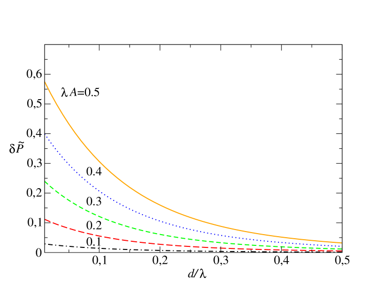
Figure 4: The plots of the (positive) difference between the rescaled pressures for uniformly and periodically (period $\lambda$) charged lines (5.42) with the same mean line charge density given by $\lambda\sigma=\frac{1}{2}$ versus the dimensionless distance between the lines $d/\lambda$. The equivalent left and right charge densities are in phase with respect to one another. The curves correspond from up to down to five values of the (dimensionless) modulation amplitude $\lambda A=0.5,0.4,0.3,0.2,0.1$.

The choice of the equivalent (positive) amplitudes

$$A_{L}=A_{R}\equiv A,\qquad\lambda A\leq\lambda\sigma=\frac{1}{2},$$ (5.38)

describes the identical left and right line charge densities which are in phase with respect to one another. The rescaled pressure (5.31) is now given by

$$\widetilde{P}\left(d/\lambda,\lambda A\right)=\pi(\lambda A)^{2}{\rm e}^{-2\pi d/\lambda}+2\frac{\partial}{\partial(d/\lambda)}g\left(d/\lambda,\lambda A\right),$$ (5.39)

where

$$g\left(d/\lambda,\lambda A\right) = \frac{1}{4\pi}\int_{0}^{2\pi}{\rm d}r\,\ln\Bigg{\{}\int_{0}^{d/\lambda}{\rm d}x^{\prime}\,{\rm e}^{-rx^{\prime}}$$ (5.40)

$$\times I_{0}\left[\lambda A\left({\rm e}^{-2\pi x^{\prime}}+{\rm e}^{-2\pi d/\lambda+2\pi x^{\prime}}\right)\right]\Bigg{\}}.$$

The numerical treatment of this result implies that, as in the case of uniformly charged lines, the pressure $\widetilde{P}$ is always positive and decays monotonously from $\infty$ at $d/\lambda\to 0$ to 0 at $d/\lambda\to\infty$. It turns out that at arbitrary distance $d/\lambda$ the pressure $\widetilde{P}$ is always smaller than the rescaled pressure of the uniformly charged lines $\sigma_{L}=\sigma_{R}=\sigma$ with $\lambda\sigma=\frac{1}{2}$,

$$\lambda^{2}\beta P_{0}(d/\lambda)=\frac{1}{\pi}\left(\frac{\lambda}{d}\right)^{2}\int_{0}^{\pi d/\lambda}{\rm d}t\,\frac{t}{\sinh t}{\rm e}^{-t}.$$ (5.41)

The (positive) difference between the rescaled pressures

$$\delta\widetilde{P}\left(d/\lambda,\lambda A\right)\equiv\lambda^{2}\beta P_{0}(d/\lambda)-\widetilde{P}\left(d/\lambda,\lambda A\right)$$ (5.42)

is pictured in figure 4 for five values of the modulation parameter (from up to down) $\lambda A=0.5,0.4,0.3,0.2,0.1$. It is seen that the pressure difference increases with increasing the dimensionless cosine amplitude of the modulated line charge density $\lambda A$ and with decreasing the dimensionless distance between the lines $d/\lambda$.

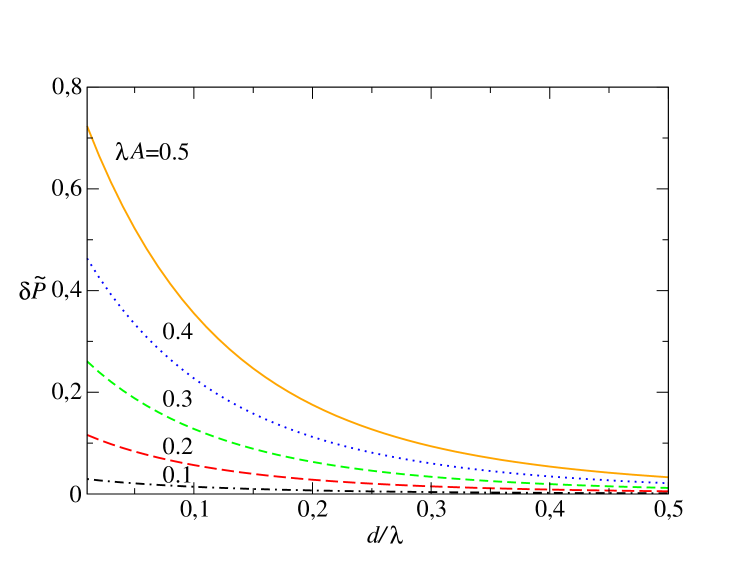
Figure 5: The same as in figure 4, but the equivalent left and right charge densities are shifted by a half-period $\lambda/2$ with respect to one another.

The choice of the amplitudes with opposite signs

$$A_{L}=-A_{R}\equiv A,\qquad\lambda A\leq\frac{1}{2},$$ (5.43)

describes the identical left and right line charge densities which are shifted in phase with respect to one another by a half-period $\lambda/2$. The rescaled pressure (5.31) is given by

$$\widetilde{P}\left(d/\lambda,\lambda A\right)=-\pi(\lambda A)^{2}{\rm e}^{-2\pi d/\lambda}+2\frac{\partial}{\partial(d/\lambda)}g\left(d/\lambda,\lambda A\right),$$ (5.44)

where

$$g\left(d/\lambda,\lambda A\right) = \frac{1}{4\pi}\int_{0}^{2\pi}{\rm d}r\,\ln\Bigg{\{}\int_{0}^{d/\lambda}{\rm d}x^{\prime}\,{\rm e}^{-rx^{\prime}}$$ (5.45)

$$\times I_{0}\left[\lambda A\left({\rm e}^{-2\pi x^{\prime}}-{\rm e}^{-2\pi d/\lambda+2\pi x^{\prime}}\right)\right]\Bigg{\}}.$$

As before, the pressure $\widetilde{P}$ is positive and decays monotonously from $\infty$ at $d/\lambda\to 0$ to 0 at $d/\lambda\to\infty$. It is always smaller than the rescaled pressure of the uniformly charged lines (5.41) taken at $\lambda\sigma=\frac{1}{2}$. The positive difference between the pressures (5.42) is pictured in figure 5 for five values of the parameter $\lambda A=0.5,0.4,0.3,0.2,0.1$. In comparison with the results in figure 4, the half-period shift in the line charge densities induces, for fixed values of the parameters $\lambda A$ and $d/\lambda$, larger differences between the pressures.

We conclude that, at any distance between two lines, the modulation of the line charge densities always leads to the diminution of the pressure in comparison with the symmetric lines charged uniformly by the same mean line charge densities.

6 Conclusion

In this paper, the system of mobile charges is put on the surface of the 2D cylinder (section 2). The particles are confined to either the semi-infinite space bounded by one circle or the finite space between two circles at distance $d$, in both cases the circles are charged inhomogeneously by a fixed line charge density. The question is how the non-uniformity of the line charge densities influences the particle density and the effective interaction between two circles.

2D one-component Coulomb fluids in thermal equilibrium have the advantage of being exactly solvable not only in the high-temperature PB limit of the coupling constant $\Gamma\to 0$ but also, in principle, at the finite free-fermion coupling $\Gamma=2$. Moreover, for the series of coupling constants $\Gamma=2\gamma$ with $\gamma$ being a positive integer, the partition function and the many-body particle densities of the 2D Coulomb system are expressible explicitly in terms of the 1D anticommuting field theory defined on a chain of sites (section 3). Specific transformations of anticommuting variables, which keep the composite form of the operators (3.2), lead to specific sum rules, i.e., exact constraints for correlators of the composite operators.

As concerns the semi-infinite geometry of one EDL (section 4), the derived sum rule for correlators of the composite operators implies the contact value theorem (4.5) valid for any $\Gamma$. Its form, which involves the particle density profile inside the whole semi-infinite region accessible to particle, is much more complicated that the one of the homogeneously charged line (4.6), which involves only the particle density at the line contact. At the free fermion coupling constant $\Gamma=2$, choosing the cosine modulation of the line charge density with period $\lambda$ (4.19), the matrix of interaction strengths between the anticommuting variables becomes diagonal under the condition (4.16) for the mean line charge density $\sigma$. This leads to the explicit form of the particle density profile (4.32). The numerical results for the ratio of the mean (averaged over the $y$-axis) values of the contact densities of counterions for the modulated and uniform line charge densities, always larger than 1 as is seen in figure 3, confirm the anticipated enhancement of the counterion density at the line due to the line charge modulation.

The effective interaction (the pressure) between two EDLs at distance $d$ is discussed in section 5. For the cosine modulation of left and right line charge densities (5.9), under the condition (5.14) for the left and right mean values of the line charge densities, the pressure at the free fermion coupling $\Gamma=2$ is given by equations (5.27) and (5.29). Restricting ourselves to the symmetric left and right mean line charge densities (5.36) with $\lambda\sigma=\frac{1}{2}$, two choices for the amplitudes of the cosine modulations are considered: $A_{L}=A_{R}\equiv A$ (the modulations are in phase, for numerical results see figure 4) and $A_{L}=-A_{R}\equiv A$ (the modulations are shifted by half-period $\lambda/2$, for numerical results see figure 5). In both cases, similarly as in the uniform case, the positive pressure is a decreasing function of the dimensionless distance between lines $d/\lambda$. In other words, the considered modulations of the line charge densities are not strong enough to induce an effective attraction between the circles in an interval of the distance $d/\lambda$. This feature does not contradict a recent study [61] dealing with finite-$N$ counterion systems on the surface of the cylinder with symmetric uniformly charged circles at couplings $\Gamma=2,3,4$ which indicates that the attraction arises somewhere between $\Gamma=2$ and $\Gamma=4$. As is seen in figures 4 and 5, the modulation of the line charge densities always decreases the pressure, which is in agreement with the expectation from the mean-field PB theory and MC simulations.

References

References

- [1] Martin Ph A 1988 Sum rules in charged fluids Rev. Mod. Phys. 60 1075–1127
- [2] Andelman D 2006 Introduction to electrostatics in soft and biological matter In: Poon, W.C.K., Andelman, D. (eds.) Soft Condensed Matter Physics in Molecular and Cell Biology vol. 6. (Taylor & Francis, New York)
- [3] Levin Y 2002 Electrostatic correlations: from Plasma to Biology Rep. Prog. Phys. 65 1577–1632
- [4] Gulbrand L, Jönsson B, Wennerström H and Linse P 1984 Electrical double layer forces. A Monte Carlo study J. Chem. Phys. 80 2221-2228
- [5] Attard P, Mitchell D J and Ninham B W 1988 Beyond Poisson-Boltzmann: Images and correlations in the electric double layer. I. Counterions only J. Chem. Phys. 88 4987–4996
- [6] Attard Ph 1996 Electrolytes and the electric double layer Adv. Chem. Phys. XCII 1–159
- [7] Messina R 2009 Electrostatics in soft matter J. Phys.: Condens. Matter 21 113102
- [8] Henderson D and Blum L 1978 Some exact results and the application of the mean spherical approximation to charged hard spheres near a charged hard wall J. Chem. Phys. 69 5441–5449
- [9] Henderson D, Blum L and Lebowitz J L 1979 An exact formula for the contact value of the density profile of a system of charged hard spheres near a charged wall J. Electroanal. Chem. 102 315–319
- [10] Blum L, Henderson D, Lebowitz J L, Gruber Ch and Martin Ph A 1981 A sum rule for an inhomogeneous electrolyte J. Chem. Phys. 75 5974–5975
- [11] Carnie S L and Chan D Y C 1981 The Stillinger-Lovett condition for non-uniform electrolytes Chem. Phys. Lett. 77 437–440
- [12] Hansen J P and Löwen H 2000 Effective interactions between electric double layers Annu. Rev. Phys. Chem. 51 209–242
- [13] Khan A, Jönsson B and Wennerström H 1985 Phase equilibria in the mixed sodium and calcium di-2-ethylhexylsulfosuccinate aqueous system. An illustration of repulsive and attractive double-layer forces J. Phys. Chem. 89 5180–5184
- [14] Kjellander R, Marčelja S and Quirk J P 1988 Attractive double-layer interactions between calcium clay particles J. Colloid Interface Sci. 126 194–211
- [15] Bloomfield V A 1991 Condensation of DNA by multivalent cations: Considerations on mechanism Biopolymers 31 1471–1481
- [16] Kékicheff P, Marčelja S, Senden T J and Shubin V E 1993 Charge reversal seen in electrical double layer interaction of surfaces immersed in 2:1 calcium electrolyte J. Chem. Phys. 99 6098–6113
- [17] Dubois M, Zemb T, Fuller N, Rand R P and Pargesian V A 1998 Equation of state of a charged bilayer system: Measure of the entropy of the lamellar–lamellar transition in DDABr J. Chem. Phys. 108 7855–7869
- [18] Kjellander R and Marčelja S 1984 Correlation and image charge effects in electric double-layers Chem. Phys. Lett. 112 49–53
- [19] Grønbech-Jensen N, Mashl R J, Bruinsma R F and Gelbart W M 1997 Counterion-Induced attraction between rigid polyelectrolytes Phys. Rev. Lett. 78 2477–2480
- [20] Boroudjerdi H, Kim Y-W, Naji A, Netz R R, Schlagberger X and Serr A 2005 Statics and dynamics of strongly charged soft matter Phys. Rep. 416 129–199
- [21] Naji A, Kanduč M, Forsman J and Podgornik R 2013 Perspective: Coulomb fluids – Weak coupling, strong coupling, in between and beyond J. Chem. Phys. 139 150901
- [22] Netz R R, Orland H 2000 Beyond Poisson-Boltzmann: Fluctuation effects and correlation functions Eur. Phys. J. E 1 203–214
- [23] Podgornik R 1990 An analytic treatment of the first-order correction to the Poisson-Boltzmann interaction free energy in the case of counter-ion only Coulomb fluid J. Phys. A: Math. Gen. 23 275–284
- [24] Moreira A G and Netz R R 2000 Strong-coupling theory for counter-ion distributions Europhys. Lett. 52 705–711
- [25] Moreira A G and Netz R R 2001 Binding of similarly charged plates with counterions only Phys. Rev. Lett. 87 078301
- [26] Netz R R 2001 Electrostatics of counter-ions at and between planar charged walls: from Poisson-Boltzmann to the strong-coupling theory Eur. Phys. J. E 5 557–574
- [27] Moreira A G and Netz R R 2002 Simulations of counterions at charged plates Eur. Phys. J. E 8 33–58
- [28] Kanduč M and Podgornik R 2007 Electrostatic image effects for counterions between charged planar walls Eur. Phys. J. E 23 265–274
- [29] Shklovskii B I 1999 Screening of a macroion by multivalent ions: Correlation-induced inversion of charge Phys. Rev. E 60 5802–5811
- [30] Levin Y, Arenzon J J and Stilck J F 1999 The nature of attraction between like-charged rods Phys. Rev. Lett. 83 2680–2680
- [31] Grosberg A Y, Nguyen T T and Shklovskii B I 2002 Colloquium: The physics of charge inversion in chemical and biological systems Rev. Mod. Phys. 74 329–345
- [32] Šamaj L and Trizac E 2011 Counterions at highly charged interfaces: From one plate to like-charge attraction Phys. Rev. Lett. 106 078301
- [33] Šamaj L and Trizac E 2011 Wigner-crystal formulation of strong-coupling theory for counterions near planar charged interfaces Phys. Rev. E 24 041401
- [34] Nordholm S 1984 Simple analysis of the thermodynamic properties of the one-component plasma Chem. Phys. Lett. 105 302–307
- [35] Forsman J 2004 A simple correlation-corrected Poisson-Boltzmann theory J. Phys. Chem. B 108 9236–9245
- [36] Šamaj L, dos Santos A P, Levin Y and Trizac E 2016 Mean-field beyond mean-field: the single particle view for moderately to strongly coupled charged fluids Soft Matter 12 8768–8773
- [37] Palaia I, Trulsson M, Šamaj L and Trizac E 2018 A correlation-hole approach to the electric double layer with counter-ions only Mol. Phys. 116 3134–3146
- [38] Israelachvili J N 1992 Intermolecular and Surface Forces 3rd edn. (Academic Press, San Diego)
- [39] Leckband D E, Helm C A and Israelachvili J 1993 The role of calcium in the adhesion and fusion of mixed lipid bilayers Biochem. 32 1127–1140
- [40] Walz J Y 1998 The effect of surface heterogeneities on colloidal forces Adv. Colloid Interface Sci. 74 119–168
- [41] Chan D Y C, Mitchell J and Ninham B W 1980 A self‐consistent study of ion adsorption and discrete charge effects in the electrical double layer J. Chem. Phys. 72 5159–5162
- [42] Kjellander R and Marčelja S 1988 Inhomogeneous Coulomb fluids with image interactions between planar surfaces. III. Distribution functions J. Chem. Phys. 88 7138–7146
- [43] Lukatsky D B, Safran S A, Lau A W C and Pincus P A 2002 Enhanced counterion localization induced by surface charge modulation Europhys. Lett. 58 785–791
- [44] Henle M L, Santangelo C D, Patel D M and Pincus P A 2004 Distribution of counterions near discretely charged planes and rods Europhys. Lett. 66 284–290
- [45] Fleck C C and Netz R. R. 2005 Counterions at disordered charged planar surfaces Europhys. Lett. 70 341–347
- [46] Lukatsky D B and Safran S A 2002 Universal reduction of pressure between charged surfaces by long-wavelength surface charge modulation Europhys. Lett. 60 629–635
- [47] Khan M O, Petris S and Chan D Y C 2005 The influence of discrete surface charges on the force between charged surfaces J. Chem. Phys. 122 104705
- [48] Šamaj L and Trizac E 2019 Electric double layers with surface charge modulations: Exact Poisson-Boltzmann solutions Phys. Rev. E 100 042611
- [49] Jancovici B 1981 Exact results for the two-dimensional one-component plasma Phys. Rev. Lett. 46 386–388
- [50] Alastuey A and Jancovici B 1981 On the classical two-dimensional one-component Coulomb plasma J. Physique 42 1–12
- [51] Jancovici B 1992 Inhomogeneous two-dimensional plasmas In: Inhomogeneous Fluids pp. 201-237 Henderson D (ed.) (Dekker, New York)
- [52] Forrester P J 1998 Exact results for two-dimensional Coulomb systems Phys. Rep. 301 235–270
- [53] Téllez G and Forrester P J 1999 Exact finite-size study of the 2d-OCP at and J. Stat. Phys. 97 489–521
- [54] Téllez G and Forrester P J 2012 Expanded Vandermonde powers and sum rules for the two-dimensional one-component plasma J. Stat. Phys. 147 825–855
- [55] Šamaj L and Percus J K 1995 A functional relation among the pair correlations of the two-dimensional one-component plasma J. Stat. Phys. 80 811–824
- [56] Šamaj L 2004 Is the two-dimensional one-component plasma exactly solvable? J. Stat. Phys. 117 131–158
- [57] Šamaj L, Wagner J and Kalinay P 2004 Translation symmetry breaking in the one-component plasma on the cylinder J. Stat. Phys. 117 159–178
- [58] Šamaj L 2015 Counter-ions near a charged wall: Exact results for disc and planar geometries J. Stat. Phys. 161 227–249
- [59] Jancovici B 1984 Surface properties of a classical two-dimensional one-component plasma: Exact results J. Stat. Phys. 34 803–815
- [60] Šamaj L 2013 Counter-ions at single charged wall: Sum rules Eur. Phys. J. E 36 100
- [61] Šamaj L 2020 Attraction of like-charged walls with counterions only: Exact results for the 2D cylinder geometry J. Stat. Phys. 181 1699–1729
- [62] Choquard Ph 1981 The two-dimensional one component plasma on a periodic strip Helv. Phys. Acta 54 332–332
- [63] Šamaj L and Trizac E 2014 Counter-ions between or at asymmetrically charged walls: 2D free-fermion point J. Stat. Phys. 156 932–947
- [64] Šamaj L 2000 Microscopic calculation of the dielectric susceptibility tensor for Coulomb fluids J. Stat. Phys. 100 949–967
- [65] Gradshteyn I S and Ryzhik I M 2000 Table of Integrals, Series, and Products 6th edn. (Academic Press, London)