Sudden change of the photon output field marks phase transitions in the quantum Rabi model

Abstract

Abstract: The experimental observation of quantum phase transitions predicted by the quantum Rabi model in quantum critical systems is usually challenging due to the lack of signature experimental observables associated with them. Here, we describe a method to identify the dynamical critical phenomenon in the quantum Rabi model consisting of a three-level atom and a cavity at the quantum phase transition. Such a critical phenomenon manifests itself as a sudden change of steady-state output photons in the system driven by two classical fields, when both the atom and the cavity are initially unexcited. The process occurs as the high-frequency pump field is converted into the low-frequency Stokes field and multiple cavity photons in the normal phase, while this conversion cannot occur in the superradiant phase. The sudden change of steady-state output photons is an experimentally accessible measure to probe quantum phase transitions, as it does not require preparing the equilibrium state.

Introduction

In quantum systems close to critical points, small variations of physical parameters can lead to drastic changes in the equilibrium-state properties Agarwal (2012); Scully and Zubairy (1997); Scully and Svidzinsky (2009); Sachdev (2011). An interesting class of quantum critical systems is provided by light-matter interaction models Cong et al. (2016); Kirton et al. (2018); Kockum et al. (2019); Forn-Díaz et al. (2019), such as the quantum Rabi Ashhab (2013); Hwang et al. (2015) and Dicke models Hepp and Lieb (1973); Wang and Hioe (1973); Emary and Brandes (2003); Lambert et al. (2004); Scully (2015); Shammah et al. (2017, 2018); Makihara et al. (2021) describing the interaction of single or many two-level atoms (atomic levels $|g\rangle$ and $|e\rangle$) with a single-model cavity. The quantum Dicke model exhibits a superradiant quantum phase transition (QPT) in the thermodynamic limit of infinite atoms Hepp and Lieb (1973); Wang and Hioe (1973); Emary and Brandes (2003); Lambert et al. (2004); Scully (2015); Shammah et al. (2017, 2018). Such a thermodynamic limit leads to some difficulties in experimentally exploring the superradiant QPTs Baumann et al. (2010, 2011); Bastidas et al. (2012); Mlynek et al. (2014); Fuchs et al. (2016); Zhang et al. (2017); Léonard et al. (2017); Zhu et al. (2020). Instead, by replacing the thermodynamic limit with a scaling of the system parameters, the quantum Rabi model described by the Hamiltonian (hereafter $\hbar=1$)

$$H_{R}=\omega a^{{\dagger}}a(|e\rangle\langle e|+|g\rangle\langle g|)+{\Omega}|e\rangle\langle e|-g(a+a^{{\dagger}})(|g\rangle\langle e|+|e\rangle\langle g|),$$ (1)

can also exhibit a superradiant QPT Ashhab (2013); Hwang et al. (2015), where $\omega$ ($\Omega$) is the cavity-mode (atomic-transition) frequency, $a$ ($a^{{\dagger}}$) is the cavity-mode annihilation (creation) operator, and $g$ is the light-matter coupling strength. We assume that the level frequency of the atomic state $|g\rangle$ is zero. This superradiant QPT has been experimentally observed Cai et al. (2021); Chen et al. (2021a) and is attracting increasing attention Puebla et al. (2016); Shen et al. (2017); Liu et al. (2017); Hwang et al. (2018); Jiang et al. (2021); Zheng et al. (2023). However, one of the most important critical phenomena in this system, i.e., a discontinuity of the derivative for the number of bare photons at the critical point, is hard to observe.

Unlike classical phase transitions, superradiant QPTs can occur when changing the system parameters at zero temperature Cong et al. (2016); Kirton et al. (2018); Shammah et al. (2017). Specifically, when $g$ approaches the critical point, it was predicted Hwang et al. (2015) that the mean photon number in the ground eigenstate of $H_{R}$ suddenly increases to infinity. This corresponds to a QPT from a normal phase (NP), where the ground state of the cavity field is not occupied, to a superradiant phase (SP), where the ground state is macroscopically occupied. However, experimentally exploring this critical phenomenon is challenging because: (i) the time required to prepare this equilibrium state diverges Hwang et al. (2015); and (ii) these photons are virtual, so cannot be directly measured Forn-Díaz et al. (2019); Kockum et al. (2019). Especially, the difficulty (i) may make transition-edge sensing protocols Garbe et al. (2020); Tsang (2013); Wang et al. (2014) not effective in detecting this kind of phase transitions.

Here we show how to overcome these problems by introducing additional low-energy levels in the quantum Rabi model and driving transitions among these levels. We show that the stimulated emission effect of the whole system can directly reflect the change of the photon-number distributions of the quantum Rabi Hamiltonian. The process can be interpreted as a multi-photon down-conversion induced by stimulated Raman transitions [i.e., a pump photon is converted into a Stokes photon and multiple cavity photons, as shown in Fig. 1(a)] Stassi et al. (2013); Huang and Law (2014); Kockum et al. (2017); Chen et al. (2021b). This parametric down-conversion process changes abruptly when the superradiant QPT occurs in the quantum Rabi Hamiltonian. Such a change can be observed by measuring the real photons continuously released from the cavity. Note that this parametric down-conversion process was initially studied by Huang et al. in 2014 for photon emission via vacuum-dressed intermediate states Huang and Law (2014). We find that such a photon emission can be useful in observing quantum critical phenomena. We predict that the steady-state output photon rate can reach $\Phi_{\rm{out}}^{\rm{ss}}\sim 4\times 10^{-3}\omega$ in the NP, then suddenly vanishes when tuning the Rabi Hamiltonian into the SP. This demonstrates a sudden change of the ground eigenstate of the quantum Rabi Hamiltonian, and indicates the occurrence of the superradiant QPT.

Results

I Superadiant quantum phase transitions

Note that the theory of the superradiant phase transition in the quantum Rabi model was developed first in 2013 Ashhab (2013) and then in 2015 Hwang et al. (2015). For clarity, we first review the theory of the superradiant phase transition in the quantum Rabi model. In the limit of $\Omega/\omega\rightarrow\infty$, following Refs. Ashhab (2013); Hwang et al. (2015), we can solve the Hamiltonian $H_{R}$ in Eq. (1) using a Schrieffer-Wolff transformation Scully and Zubairy (1997); Agarwal (2012):

$$U_{\rm{SW}}=\exp{\left[\left(\frac{g}{\Omega}\right)\left(a+a^{{\dagger}}\right)\left(|e\rangle\langle g|-|g\rangle\langle e|\right)\right]}.$$ (2)

For the transformed Hamiltonian, the transitions between the ground- and excited-qubit-state subspaces $\left\{|n\rangle|g\rangle\right\}$ and $\left\{|n\rangle|e\rangle\right\}$ are negligible. Thus, we perform a projection $\langle g|U_{\rm SW}^{{\dagger}}H_{R}U_{\rm SW}|g\rangle$, resulting in

$$H_{\rm{np}}=\omega a^{{\dagger}}a-\frac{\omega g_{c}^{2}}{4}\left(a+a^{{\dagger}}\right)^{2}+O(g_{c}^{2}\omega/\Omega),$$ (3)

where

$$g_{c}=2g/\sqrt{\omega\Omega},$$

is the normalized coupling strength and $O(g_{c}^{2}\omega/\Omega)$ denotes negligible higher-order terms. The excitation energy of $H_{\rm np}$ is

$$\varepsilon_{\rm{np}}=\omega\sqrt{1-g_{c}^{2}},$$

which is real only for $g_{c}\leq 1$ and vanishes at $g_{c}=1$, i.e., in the NP Hwang et al. (2015). The ground eigenstate of $H_{\rm{np}}$ is $|E_{0}\rangle=S(r_{\rm{np}})|0\rangle$, with

$$S(r_{\rm{np}})=\exp\left[\frac{r_{\rm{np}}}{2}\left(a^{{\dagger}2}-a^{2}\right)\right],\ \ \ \ \ \ {\rm and}\ \ \ \ \ \ \ r_{\rm{np}}=-\frac{1}{4}\ln\left(1-g_{c}^{2}\right).$$ (4)

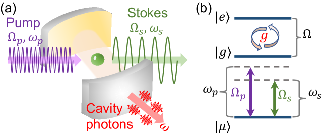
Figure 1: Sketch and atomic level structure of the protocol. (a) Sketch of the parametric down-conversion process in an atom-cavity system. A pump pulse of frequency $\omega_{p}$ is converted into a Stokes pulse of frequency $\omega_{s}$ and multiple cavity photons of frequency $\omega$. (b) Level structure of the atom. The upper two atomic levels $|g\rangle$ and $|e\rangle$ are ultrastrongly coupled to the cavity mode with strength $g$. The lower two levels $|g\rangle$ and $|\mu\rangle$ are off-resonantly driven by a composite pulse of two frequencies ($\omega_{p}$ and $\omega_{s}$) and two amplitudes ($\Omega_{p}$ and $\Omega_{s}$).

For $g_{c}>1$ and

$$\alpha=\frac{1}{2}\sqrt{\frac{\Omega}{\omega}\left(g_{c}^{2}-g_{c}^{-2}\right)}\ \geq 0,$$ (5)

after displacing the cavity field with displacement operators

$$D(\pm\alpha)=\exp\left[\pm\alpha\left(a^{{\dagger}}-a\right)\right],$$ (6)

we can employ the same procedure in deriving $H_{\rm{np}}$ to obtain the Hamiltonian in the SP:

$$H_{\rm{sp}}\approx\omega a^{{\dagger}}a-\frac{\omega}{4g_{c}^{4}}\left(a+a^{{\dagger}}\right)^{2}+{\frac{\Omega}{2}\left(1-g_{c}^{2}\right)+\omega\alpha^{2}}.$$ (7)

The excitation energy of $H_{\rm{sp}}$ is $\varepsilon_{\rm{sp}}=\omega\sqrt{1-g_{c}^{-4}}$ and the ground eigenstate of $H_{\rm{sp}}$ is $S(r_{\rm{sp}})|0\rangle$, with

$$r_{\rm{sp}}=-\frac{1}{4}\ln\left(1-g_{c}^{-4}\right).$$ (8)

Thus, in the lab frame, $H_{R}$ has two degenerate ground eigenstates

$$|E_{0}\rangle=D(\pm\alpha)S(r_{\rm{sp}})|0\rangle|\!\downarrow\rangle_{\pm},$$ (9)

where $|\!\downarrow\rangle_{\pm}$ are the ground eigenstates of

$$H_{\pm}=\Omega|e\rangle\langle e|\mp 2g\alpha(|e\rangle\langle g|+|g\rangle\langle e|).$$ (10)

This is because two different displacement parameters $\pm\alpha$ result in an indentical spectrum Ashhab (2013).

II Demonstrating the critical phenomenon

The sudden change of $\bar{n}_{0}=\langle E_{0}|a^{{\dagger}}a|E_{0}\rangle$ at the critical point $g_{c}=1$ is the most important benchmark of the superradiant QPT. Specifically, when $\Omega/\omega\rightarrow\infty$, the derivative $d\bar{n}_{0}/dg_{c}$ is discontinuous at the critical point $g_{c}=1$ [see Fig. 2(a)], indicating the occurrence of the superradiant QPT. However, observing this critical phenomenon is still challenging in experiments mainly because: (i) it is difficult to prepare the ground state $|E_{0}\rangle$ at the critical point; (ii) one cannot adiabatically tune control parameters across the critical point Cai et al. (2021); Chen et al. (2021a) since the energy gap mostly closes at the critical point; and (iii) the photons in the ground eigenstate $|E_{0}\rangle$ are virtual and cannot be directly measured Forn-Díaz et al. (2019); Kockum et al. (2019).

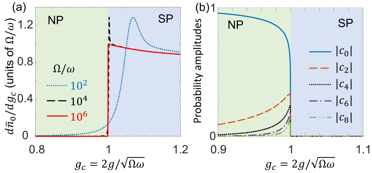
Figure 2: Sudden change of photon number distribution. (a) Derivative $d\bar{n}_{0}/dg_{c}$ of the virtual cavity excitation number $\bar{n}_{0}=\langle E_{0}|a^{{\dagger}}a|E_{0}\rangle$ calculated for different frequency rate $\Omega/\omega$. (b) Probability amplitudes $|c_{2k}|$ of the states $|2k\rangle|g\rangle$ in the eigenstate $|E_{0}\rangle$ of $H_{R}$ in Eq. (1) when $\Omega=10^{6}\omega$ approximatively satisfying the condition $\Omega/\omega\rightarrow\infty$. The green- and blue-shaded areas denote the normal phase (NP) and the superradiant phase (SP), respectively.

Instead, in this manuscript, we propose to measure the sudden change of the photon number distributions of $|E_{0}\rangle$, i.e., the probability amplitudes $c_{k}(g_{c})=\langle g|\langle k|E_{0}\rangle$. This is equivalent to measuring the change of $\langle E_{0}|a^{{\dagger}}a|E_{0}\rangle$ because it can be calculated using the photon number distributions. In the $\Omega/\omega\rightarrow\infty$ limit, it is expected that $\alpha\rightarrow\infty$ and $r_{\rm{sp}}\neq 0$ when $g_{c}>1$. Thus, when $g_{c}$ is tuned across the critical point, there is a sudden change in the amplitude $c_{2k}$:

$$|c_{2k}(g_{c})|\xrightarrow{\ g_{c}=1^{-}}\left|\frac{\left[-\tanh(r_{\rm np})\right]^{k}\sqrt{(2k)!}}{2^{k}k!\sqrt{\cosh(r_{\rm np})}}\right|>0,$$ (11)

$$|c_{2k}(g_{c})|\xrightarrow{\ g_{c}=1^{+}}\left|\frac{(\tanh r_{\rm sp})^{k}\exp\left[-\frac{\alpha^{2}}{2}(1+\tanh r_{\rm sp})\right]}{2^{k}\sqrt{(2k)!\cosh r_{\rm sp}}}\mathcal{H}_{{}_{n}}(x)\right|\longrightarrow 0,$$ (12)

where $\mathcal{H}_{n}(x)$ are the Hermite polynomials with

$$x=\frac{\alpha\exp{(r_{\rm sp})}}{\sqrt{\sinh 2r_{\rm sp}}}.$$ (13)

Such a change is obvious when $k$ is small, because $|c_{2k}(g_{c}\rightarrow 1^{-})|$ is significant as shown in Fig. 2(b). Especially, for $k<5$, the components of the few-photon states in the eigenstate $|E_{0}\rangle$ of $H_{R}$ suddenly vanish when $g_{c}$ is tuned across the critical point [see Fig. 2(b)]. This coincides with the sudden changes of the photon number $\bar{n}_{0}$ and its derivative $d\bar{n}_{0}/dg_{c}$ [see the red-solid curve in Fig. 2(a)].

To demonstrate the sudden change of $c_{2k}$, following the idea in Ref. Huang and Law (2014), we introduce a third low-energy level $|\mu\rangle$ with level frequency $\omega_{\mu}<0$ for the atom [see Fig. 1(b)]. We assume that $|\omega_{\mu}|\gg\omega$, so that the state $|\mu\rangle$ is far off-resonance to the cavity bare frequency. The atom-cavity interaction becomes

$$H_{0}=H_{R}+\omega_{\mu}|\mu\rangle\langle\mu|+\omega a^{{\dagger}}a|\mu\rangle\langle\mu|,$$ (14)

whose eigenstates $|\xi_{j}\rangle$ can be separated into: (i) the noninteracting sectors $|\mu_{n}\rangle=|n\rangle|\mu\rangle$ with eigenvalues $n\omega+\omega_{\mu}$; and (ii) the eigenstates $|E_{m}\rangle$ of $H_{R}$ with eigenvalues $E_{m}$ ($j,n,m=0,1,2,\ldots$). The ground state of the whole system becomes $|\mu_{0}\rangle$, which is the initial state for the system dynamics hereafter.

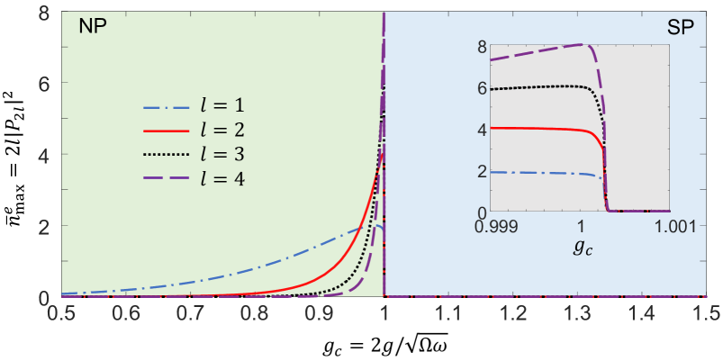
Figure 3: Critical phenomenon. Theoretical prediction of the maximum photon number of the system after a finite-time evolution, according to Eqs. (17) and (18). For $\Xi\rightarrow 0$, we impose $t=10^{6}/\omega$ when $\pi/\Xi\rightarrow\infty$, to avoid an infinite evolution time in the coherent dynamics. Parameters are: $\Omega=10^{6}\omega$, $\omega_{\mu}=E_{0}-\left[2(n_{d}-l)+0.25\right]\omega$, $\Omega_{p}=0.005(E_{2}-E_{0})$, and $\Omega_{s}=2\Omega_{p}$. For simplicity, we choose $n_{d}=2+l$ in the simulation.

Then, as shown in Fig. 1, we employ a composite pulse to drive the atomic transition $|\mu\rangle\leftrightarrow|g\rangle$:

$$H_{D}=\left[\Omega_{p}\cos(\omega_{p}t)+\Omega_{s}\cos(\omega_{s}t)\right]\left(|\mu\rangle\langle g|+|g\rangle\langle\mu|\right),$$ (15)

where $\Omega_{p,(s)}$ and $\omega_{p,(s)}$ are the driving amplitude and frequency, respectively. Focusing on the changes of few-photon components ($k<5$), we choose $\omega_{p}=E_{0}-\omega_{\mu}$ and $\omega_{s}=E_{0}-\omega_{\mu}-2l\omega$, for $l=1,2,\ldots$, resulting in the resonant transitions $|\mu_{0}\rangle\leftrightarrow|E_{0}\rangle\leftrightarrow|\mu_{2l}\rangle$ in the subspace $\{|\xi_{j}\rangle\}$. Specifically, for weak drivings $\Omega_{p,(s)}\ll|E_{2}-E_{0}|$, the system dynamics is understood as the Raman transitions described by the effective Hamiltonian

$$H_{\rm{eff}}=\frac{1}{2}\left[c_{0}\Omega_{p}|\mu_{0}\rangle+c_{2l}\Omega_{s}|\mu_{2l}\rangle\right]\langle E_{0}|+{\rm{h.c.}},$$ (16)

which is obtained by performing $e^{iH_{0}t}H_{D}e^{-iH_{0}t}$ and neglecting fast-oscillating terms under the rotating-wave approximation (see Supplementary Note 1 for more details). Hereafter, we omit the explicit $g_{c}$ dependence of all the probability amplitudes $c_{k}$ for simplicity. The dynamics governed by $H_{\rm{eff}}$ can be interpreted as a multi-photon down-conversion process [see Fig. 1(a)], with an efficiency controllable by the coefficients $c_{0}$ and $c_{2l}$. When the initial state is $|\mu_{0}\rangle$, the probability amplitude of the state $|\mu_{2l}\rangle$ at time $t$ reads

$$P_{2l}=\frac{c_{0}\Omega_{p}c_{2l}\Omega_{s}}{4\Xi^{2}}\left[\cos{\left(\Xi t\right)-1}\right],\ \ \ \ {\rm with}\ \ \ \ \Xi^{2}=\frac{1}{4}\left[\left(c_{0}\Omega_{p}\right)^{2}+\left(c_{2l}\Omega_{s}\right)^{2}\right].$$ (17)

Choosing $t=\pi/\Xi$, the probability amplitude$P_{2l}$ and the mean photon number of the system both reach their maximum values. Then, as long as $\Omega_{p}\neq 0$ and $\Omega_{s}\neq 0$, $P_{2l}$ is measurable because $c_{0}$ and $c_{2l}$ are significant. Accordingly, the theoretical prediction of the maximum photon number of the system after a finite-time evolution is

$$\bar{n}_{\rm max}^{e}=2l|P_{2l}(t)|^{2}=2l\left|\frac{2c_{0}\Omega_{p}c_{2l}\Omega_{s}}{\left(c_{0}\Omega_{p}\right)^{2}+\left(c_{2l}\Omega_{s}\right)^{2}}\right|^{2}.\ \ \ \ \ \ \ \ \ \ \ ({\rm where}\ t=\pi/\Xi)$$ (18)

However, when $g_{c}$ is tuned across the critical point, the needed evolution time to achieve the maximum photon number tends infinite due to $\Xi\rightarrow 0$. To avoid such an infinite-time evolution, we impose $t\leq 10^{6}/\omega$ in this protocol when $\Xi\rightarrow 0$. In this limit, we obtain $P_{2l}\rightarrow 0$ because $\cos(\Xi t)\rightarrow 1$ according to Eq. (17). Therefore, as shown in Fig. 3, we theoretically predict a sudden change of the mean photon number when $g_{c}\rightarrow 1$, indicating the occurrence of the superradiant QPT.

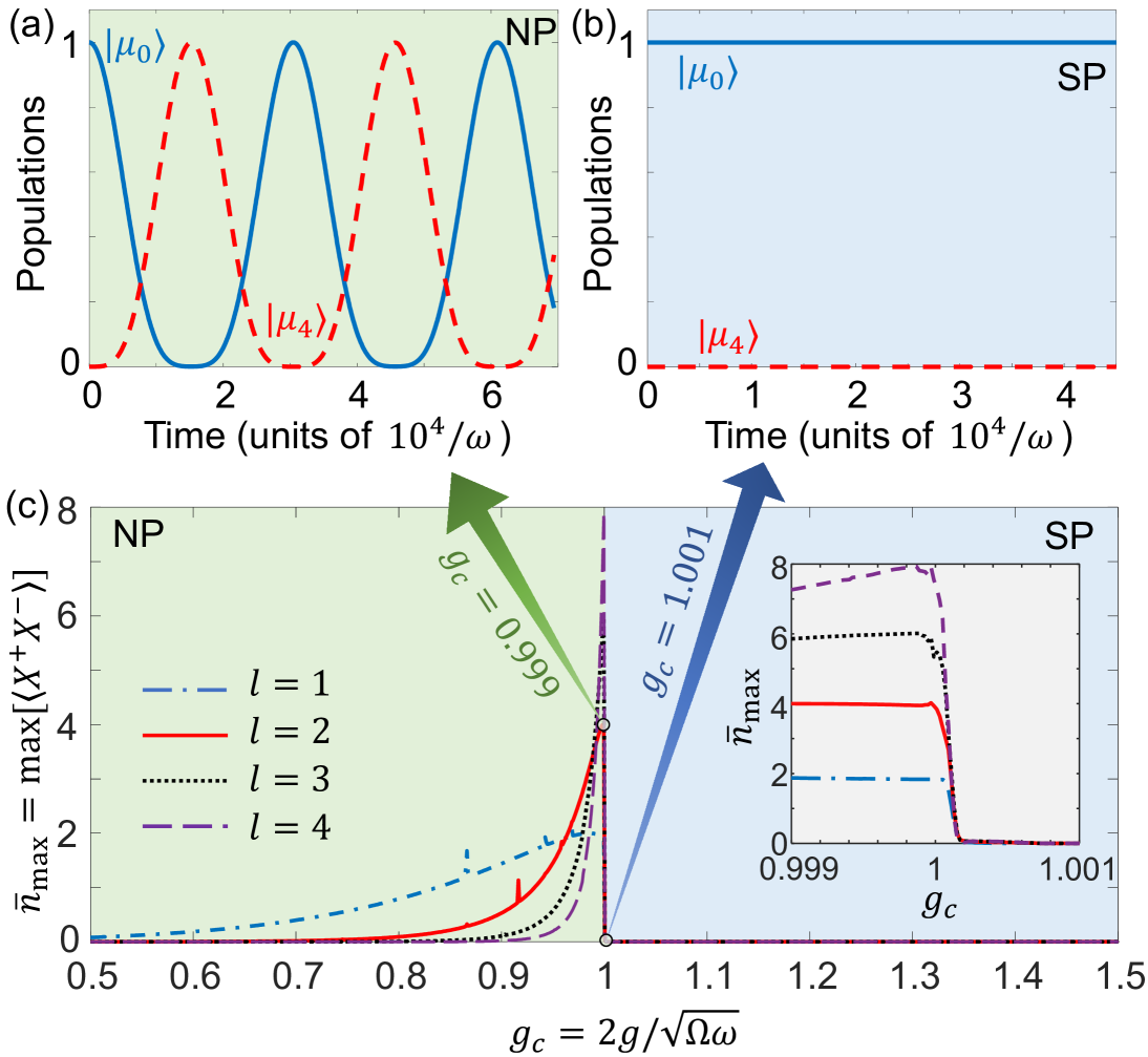
Figure 4: Dynamics of the model. Populations of the ground state $|\mu_{0}\rangle$ and the four-photon state $|\mu_{4}\rangle$ in (a) the normal phase (NP, green-shaded area) for $g_{c}=0.999$, and (b) the superradiant phase (SP, blue-shaded area) for $g_{c}=1.001$, calculated for the total Hamiltonian $H_{\rm{tot}}=H_{0}+H_{D}$. (c) Maximum value ($\bar{n}_{\rm{max}}$ at the time $t=\pi/\Xi$) over time of the mean photon number in the evolution governed by $H_{\rm{tot}}$ for $l=1,2,3,4$. Parameters are the same as those in Fig. 3. Here, $n_{d}\geq l$ is used to tune the driving frequencies $\omega_{p}$ and $\omega_{s}$; and for simplicity, we choose $n_{d}=2+l$ in the simulation. The eigenvalues $E_{0}$ and $E_{2}$ can be numerically calculated. The level frequency $\omega_{\mu}$ is chosen so that the state $|E_{0}\rangle$ is the highest level in the dynamical evolution and the state $|\mu\rangle$ is off-resonant to the cavity bare frequency. Thus, the system only has real cavity photons contributed by the state $|\mu_{2l}\rangle$.

This demonstration can be interpreted as a partial quantum process tomography, which starts at preparing the initial state $|\mu_{0}\rangle$ and fixing $g_{c}$ to a specific value, e.g., $g_{c}=0.999$. Then, turning on the drivings, one can detect the system dynamics [see the example in Fig. 4(a)]. After the detection, the drives are turned off and the system is prepared to the state $|\mu_{0}\rangle$. The next step is tuning $g_{c}$ to another value (e.g., $g_{c}=1.001$) through adjusting the frequencies $\Omega$ and $\omega$. Thus, after the energy spectrum of the system stabilizes, one can turn on the drivings again and detect the system dynamics [see the example in Fig. 4(b)]. By repeating these processes, we can know the system dynamics for an arbitrary $g_{c}$ and demonstrate the critical phenomenon as shown in Fig. 4(c), which shows the maximum value $\bar{n}_{\rm{max}}$ of the mean photon number of the system in the evolution. Note that the mean photon number is no longer $\bar{n}=\langle a^{{\dagger}}a\rangle$, but $\bar{n}=\langle X^{-}X^{+}\rangle$, where $X^{+}$ ($X^{-}$) is the positive (negative) frequency component of the quadrature operator $X=a+a^{{\dagger}}$ Ciuti and Carusotto (2006); Ridolfo et al. (2012); Kockum et al. (2019); Forn-Díaz et al. (2019). Otherwise, because of $\langle E_{0}|a^{{\dagger}}a|E_{0}\rangle\neq 0$, an observation of the stream of photons in the eigenstate $|E_{0}\rangle$ of the Rabi model would give rise to a perpetuum mobile behavior Ciuti and Carusotto (2006); Stassi et al. (2013). Because these photons can be emitted and detected in a dissipative dynamics, a measurement of the population dynamics is not necessary.

Using the corresponding input-output theory Ridolfo et al. (2012); Huang and Law (2014), we apply

$$X^{+}=\sum_{j,j^{\prime}}\langle\xi_{j^{\prime}}|\left(a+a^{{\dagger}}\right)|\xi_{j}\rangle|\xi_{j^{\prime}}\rangle\langle\xi_{j}|,$$ (19)

and $X^{-}=\left(X^{+}\right)^{{\dagger}}$ with $j^{\prime}<j$. Here, Eq. (19) describes that a photon emission from the cavity is associated with the transition from a high-energy eigenstate $|\xi_{j}\rangle$ to a low-energy eigenstate $|\xi_{j^{\prime}}\rangle$ of $H_{0}$. Note that in the subspace $\{|\mu_{n}\rangle\}$, we can obtain $\sum_{n}|\mu_{n}\rangle\langle\mu_{n}|X^{+}\sum_{m}|\mu_{m}\rangle\langle\mu_{m}|=|\mu\rangle\langle\mu|\otimes a$. That is, the photons in the states $|\mu_{2l}\rangle$ are real cavity photons, thus,

$$X^{-}X^{+}|\mu_{2l}\rangle\equiv|\mu\rangle\langle\mu|\otimes a^{{\dagger}}a|\mu_{2l}\rangle=a^{{\dagger}}a|2l\rangle|\mu\rangle.$$ (20)

Therefore, the system has maximum real photons at the time $t=\pi/\Xi$, when the state $|\mu_{2l}\rangle$ is maximally populated according to Eq. (17). Figure 4(c) shows that $\bar{n}_{\rm{max}}$ reaches a maximum when $g_{c}\rightarrow 1^{-}$, indicating a rapid increase of the mean photon number near the critical point. Then, when $g_{c}$ is tuned across the critical point, the photons suddenly vanish. The inset of Fig. 4 shows such changes more clearly, where we can see that $\bar{n}_{\rm{max}}$ changes sharply when slightly increasing $g_{c}$ from $g_{c}=1$ to $g_{c}=(1+10^{-4})$, demonstrating a sudden change of the photon-number distributions in $|E_{0}\rangle$ (see also Supplementary Note 1). Obviously, the actual dynamics of the system shown in Fig. 4(c) coincides very well with the effective one shown in Fig. 3. As an example for $l=2$, when $g_{c}=0.99999$, the theoretical prediction of the maximum photon number is $\bar{n}_{\rm max}^{e}\simeq 3.89$, and the actual number is $\bar{n}_{\rm max}\simeq 3.93$. When we change $g_{c}$ to $g_{c}=1.0003$, the theoretical prediction becomes $\bar{n}_{\rm max}^{e}\simeq 0.0018$ and the actual number is $\bar{n}_{\rm max}\simeq 0.04$. Both close to zero, indicating a sudden change of the mean photon number at the critical point. The sudden change in $\bar{n}_{\rm{max}}$ can be easily detected experimentally by measuring the rate of photons transmitted out of the cavity. Note that numerical results for actual dynamical evolution in this manuscript are obtained using the total Hamiltonian $H_{\rm{tot}}=H_{0}+H_{D}$ without approximations.

III Output photon rate

A proper generalized input-output relation in the ultrastrong-coupling regime determines the output cavity photon rate Stassi et al. (2013); Huang and Law (2014) by

$$\Phi_{\rm{out}}=\kappa{\rm{Tr}}\left[X^{-}X^{+}\rho\right].$$ (21)

Here, $\kappa$ is the cavity decay rate and $\rho$ is the density matrix obeying the following master equation at zero temperature Kockum et al. (2019); Forn-Díaz et al. (2019),

$$\dot{\rho}=i\left[\rho,H_{\rm{tot}}\right]+\sum_{\nu=1}^{3}\sum_{j,j^{\prime}<j}\Gamma_{jj^{\prime}}^{(\nu)}\left\{\mathcal{D}\left[|\xi_{j^{\prime}}\rangle\langle\xi_{j}|\right]\rho\right\},$$ (22)

where $H_{\rm{tot}}=H_{0}+H_{D}$ is the total Hamiltonian and

$$\mathcal{D}[o]\rho=o\rho o^{{\dagger}}-\frac{1}{2}\left(o^{{\dagger}}o\rho+\rho o^{{\dagger}}o\right),$$ (23)

is the Lindblad superoperator. The relaxation coefficients $\Gamma_{jj^{\prime}}^{(\nu)}$ can be written in compact forms as

$$\Gamma_{jj^{\prime}}^{(1)}= \gamma_{1}|\langle\xi_{j^{\prime}}|(|\mu\rangle\langle g|+|g\rangle\langle\mu|)|\xi_{j}\rangle|^{2},$$ (24)

$$\Gamma_{jj^{\prime}}^{(2)}= \gamma_{2}|\langle\xi_{j^{\prime}}|(|g\rangle\langle e|+|e\rangle\langle g|)|\xi_{j}\rangle|^{2},$$ (25)

$$\Gamma_{jj^{\prime}}^{(3)}= \kappa|\langle\xi_{j^{\prime}}|(a+a^{{\dagger}})|\xi_{j}\rangle|^{2},$$ (26)

where $\gamma_{1,(2)}$ is the spontaneous emission rate of the transition $|g\rangle\rightarrow|\mu\rangle$ ($|e\rangle\rightarrow|g\rangle$).

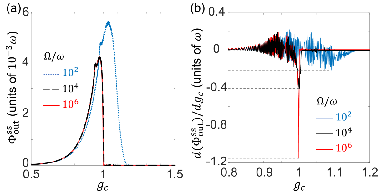
Figure 5: Photon output field. (a) Steady-state output photon rates $\Phi_{\rm{out}}^{\rm{ss}}=\Phi_{\rm{out}}|_{t\rightarrow\infty}$ defined in Eq. (21), and (b) the corresponding derivative $d\left(\Phi_{\rm{out}}^{\rm{ss}}\right)/dg_{c}$ versus $g_{c}$ for $l=2$. Dissipation rates are $\kappa=\gamma_{1}=\gamma_{2}=0.01\omega$. We choose relatively strong driving fields, i.e., $\Omega_{p}=0.05(E_{2}-E_{0})$ and $\Omega_{s}=2\Omega_{p}$, to achieve relatively large output photon rates. Strong driving fields may cause small errors (via counter-rotating effects) in obtaining the effective Hamiltonian $H_{\rm{eff}}$, leading to oscillations in $\Phi_{\rm{out}}^{\rm{ss}}$. These small errors do not affect the observation of the critical phenomenon, i.e., an extremum of $d\left(\Phi_{\rm{out}}^{\rm{ss}}\right)/dg_{c}$ at $g_{c}\rightarrow 1^{+}$. The blue, black, and red curves are plotted using frequency ratios $\Omega/\omega=10^{2}$, $\Omega/\omega=10^{4}$, and $\Omega/\omega=10^{6}$, respectively. Other parameters are the same as those in Fig. 4.

The steady-state output field can remain unchanged for a long time. This can reduce the difficulties in experiments to measure the emitted photons. Taking $l=2$ as an example, in Fig. 5(a), we show the steady-state output photon rates $\Phi_{\rm{out}}^{\rm{ss}}=\Phi_{\rm{out}}|_{t\rightarrow\infty}$, which is independent of the initial state. Focusing on $\Omega/\omega=10^{4}$ [the black-solid curve in Fig. 5(a)], the peak value of steady-state output photon rate can reach $\Phi_{\rm{out}}^{\rm{ss}}\gtrsim 4\times 10^{-3}\omega$ in the NP near the critical point when the dissipation rates are $\kappa=\gamma_{1}=\gamma_{2}=0.01\omega$. We can choose $\omega\sim 2\pi\times 5~{}$MHz and $\Omega\sim 2\pi\times 50$ GHz Yoshihara et al. (2016); Chen et al. (2017), the cavity can transmit $\sim 1.25\times 10^{5}$ photons per second, which is detectable in cavity- and circuit-QED systems. The coupling strength is $g\sim 2\pi\times 250$ MHz, and the driving amplitudes are $\Omega_{p}\gtrsim 2\pi\times 0.5$ kHz and $\Omega_{s}\gtrsim 2\pi\times 1$ kHz, which are feasible in current experiments Gu et al. (2017); Forn-Díaz et al. (2019); Kockum et al. (2019); Krantz et al. (2019); Kjaergaard et al. (2020); Kwon et al. (2021). When the parameter $g_{c}$ crosses the critical point, suddenly there is no photon released from the cavity. This indicates the drastic change of the photon number distributions and the occurrence of the QPT. The curves in Fig. 5(a) coincide well with those in Fig. 2(a), proving that the steady-state output field is a good signature of the superradiant QPT.

IV Finite-frequency effect

As mentioned above, for finite frequencies of $\Omega$ and $\omega$, the higher-order terms $O(\omega g_{c}^{2}/\Omega)$ cannot be ideally neglected but modify the eigenvalues and eigenstates of $H_{R}$ near the critical point. The influence of this finite-frequency effect is shown in Fig. 5. The first-order derivatives of $\Phi_{\rm{out}}^{\rm{ss}}$ versus $g_{c}$ are shown in Fig. 5(b). For $\Omega/\omega=10^{4}$ [black-solid curve in Fig. 5(b)] and $\Omega/\omega=10^{6}$ [red-solid curve in Fig. 5(b)], we can see deep thin dips near the critical point of $g_{c}=1$, indicating the sudden changes of output photon rates. For $\Omega/\omega=10^{2}$, the phenomenon becomes less pronounced [see the blue-solid curve in Fig. 5(b)].

Discussion

Our protocol does not need to control a parameter to adiabatically approach the critical point. Also, we do not need to prepare the equilibrium state, which is challenging in experiments because the time required diverges Hwang et al. (2015); Garbe et al. (2020). The critical phenomenon can be translated to a sudden change of the output photon rate, which can be easily detected in experiments. Thus, our protocol could be efficient to observe the critical phenomenon of the sudden change of photon number distributions in a superradiant QPT. Moreover, unlike dissipative phase transitions Baumann et al. (2010); Zhang et al. (2017); Klinder et al. (2015); Léonard et al. (2017); Minganti et al. (2021a, b), the drivings and dissipation in this manuscript are only used for quantum measurements and do not affect the QPT.

Our protocol could be implemented with superconducting circuits, which have realized the ultra- and deep-strong couplings between a single atom and a single-mode cavity Niemczyk et al. (2010); Forn-Díaz et al. (2010); Yoshihara et al. (2016, 2017); Chen et al. (2017); Bosman et al. (2017); Yoshihara et al. (2018). One can couple, e.g., a flux qubit Gu et al. (2017); Forn-Díaz et al. (2019); Kockum et al. (2019); Krantz et al. (2019); Kjaergaard et al. (2020); Kwon et al. (2021), with a lumped-element resonator via Josephson junctions to reach a coupling strength of $g/2\pi\sim 1$ GHz Yoshihara et al. (2016); Chen et al. (2017). To reduce the cavity frequency to $\omega=2\pi\times 5$ MHz, one can use an array of dc superconducting quantum interference devices Liao et al. (2010) instead of the lumped-element resonator (see Supplementary Note 2). The level structure of the atom can be realized by adjusting the external magnetic flux through the qubit loop Stassi et al. (2013); Huang and Law (2014); Stefano et al. (2017). Moreover, simulated quantum Rabi models Forn-Díaz et al. (2019); Kockum et al. (2019); Ballester et al. (2012); Lv et al. (2018); Qin et al. (2018); Leroux et al. (2018); Sánchez Muñoz et al. (2020); Chen et al. (2021c), which work in the rotating frames of the Jaynes-Cummings models, can be another possible implementation of our protocol (see also Supplementary Note 3).

Conclusion

We have investigated a method to observe quantum critical phenomena: a sudden change of photon number distributions in a quantum phase transition exhibited by the quantum Rabi model. We can interpret the system dynamics as a multi-photon down-conversion process and study the outputs near the critical point. When the normalized coupling strength $g_{c}$ is tuned across the critical point, the output of the system changes abruptly. This reflects a sudden change of the eigenstate $|E_{0}\rangle$ of the quantum Rabi model. Specifically, for the Rabi Hamiltonian in the NP, a pump pulse can be converted into a Stokes pulse and multiple cavity photons, while in the SP, it cannot. One can observe such a change by measuring the photons emitted out of the cavity continuously in the steady state. Moreover, for finite frequencies, we demonstrate that a small frequency ratio $\Omega/\omega$ may lead to the disappearance of the critical phenomenon. We expect that our method can provide a useful tool to study various critical phenomena exhibited by quantum phase transitions without preparing their equilibrium states.

Author contributions

Y.-H.C. conceived and developed the idea. Y.Q., A.M., N.L., and R.S. analyzed the data and performed the numerical simulations, with help from S.-B.Z. and W.Q.. Y.-H.C., Y.X., and F.N cowrote the paper with feedback from all authors.

Data availability

The data used for obtaining the presented numerical results as well as for generating the plots is available on request. Please refer to yehong.chen@fzu.edu.cn

Competing interests

The authors declare that they have no competing interests.

Reference

References

- Agarwal (2012) G. S. Agarwal, Quantum Optics (Cambridge University Press, Cambridge, England, 2012).
- Scully and Zubairy (1997) M. O. Scully and M. S. Zubairy, Quantum Optics (Cambridge University Press, Cambridge, England, 1997).
- Scully and Svidzinsky (2009) M. O. Scully and A. A. Svidzinsky, “The super of superradiance,” Science 325, 1510–1511 (2009).
- Sachdev (2011) S. Sachdev, Quantum Phase Transitions (Cambridge University Press, Cambridge, England, 2011).
- Cong et al. (2016) K. Cong, Q. Zhang, Y. Wang, G. T. Noe, A. Belyanin, and J. Kono, “Dicke superradiance in solids [invited],” J. Opt. Soc. Am. B 33, C80 (2016).
- Kirton et al. (2018) P. Kirton, M. M. Roses, J. Keeling, and E. G. D. Torre, “Introduction to the Dicke model: From equilibrium to nonequilibrium, and ,” Adv. Quant. Tech. 2, 1800043 (2018).
- Kockum et al. (2019) A. F. Kockum, A. Miranowicz, S. De Liberato, S. Savasta, and F. Nori, “Ultrastrong coupling between light and matter,” Nat. Rev. Phys. 1, 19–40 (2019).
- Forn-Díaz et al. (2019) P. Forn-Díaz, L. Lamata, E. Rico, J. Kono, and E. Solano, “Ultrastrong coupling regimes of light-matter interaction,” Rev. Mod. Phys. 91, 025005 (2019).
- Ashhab (2013) S. Ashhab, “Superradiance transition in a system with a single qubit and a single oscillator,” Phys. Rev. A 87, 013826 (2013).
- Hwang et al. (2015) M.-J. Hwang, R. Puebla, and M. B. Plenio, “Quantum phase transition and universal dynamics in the Rabi model,” Phys. Rev. Lett. 115, 180404 (2015).
- Hepp and Lieb (1973) K. Hepp and E. H. Lieb, “On the superradiant phase transition for molecules in a quantized radiation field: the Dicke maser model,” Ann. Phys. 76, 360–404 (1973).
- Wang and Hioe (1973) Y. K. Wang and F. T. Hioe, “Phase transition in the Dicke model of superradiance,” Phys. Rev. A 7, 831–836 (1973).
- Emary and Brandes (2003) C. Emary and T. Brandes, “Quantum chaos triggered by precursors of a quantum phase transition: The Dicke model,” Phys. Rev. Lett. 90, 044101 (2003).
- Lambert et al. (2004) N. Lambert, C. Emary, and T. Brandes, “Entanglement and the phase transition in single-mode superradiance,” Phys. Rev. Lett. 92, 073602 (2004).
- Scully (2015) M. O. Scully, “Single photon subradiance: Quantum control of spontaneous emission and ultrafast readout,” Phys. Rev. Lett. 115, 243602 (2015).
- Shammah et al. (2017) N. Shammah et al., “Superradiance with local phase-breaking effects,” Phys. Rev. A 96, 023863 (2017).
- Shammah et al. (2018) N. Shammah et al., “Open quantum systems with local and collective incoherent processes: Efficient numerical simulations using permutational invariance,” Phys. Rev. A 98, 063815 (2018).
- Makihara et al. (2021) T. Makihara et al., “Ultrastrong magnon–magnon coupling dominated by antiresonant interactions,” Nat. Commun. 12 (2021).
- Baumann et al. (2010) K. Baumann, C. Guerlin, F. Brennecke, and T. Esslinger, “Dicke quantum phase transition with a superfluid gas in an optical cavity,” Nature (London) 464, 1301–1306 (2010).
- Baumann et al. (2011) K. Baumann, R. Mottl, F. Brennecke, and T. Esslinger, “Exploring symmetry breaking at the Dicke quantum phase transition,” Phys. Rev. Lett. 107, 140402 (2011).
- Bastidas et al. (2012) V. M. Bastidas, C. Emary, B. Regler, and T. Brandes, “Nonequilibrium quantum phase transitions in the Dicke model,” Phys. Rev. Lett. 108, 043003 (2012).
- Mlynek et al. (2014) J. A. Mlynek, A. A. Abdumalikov, C. Eichler, and A. Wallraff, “Observation of Dicke superradiance for two artificial atoms in a cavity with high decay rate,” Nat. Commun. 5 (2014).
- Fuchs et al. (2016) S. Fuchs, J. Ankerhold, M. Blencowe, and B. Kubala, “Non-equilibrium dynamics of the Dicke model for mesoscopic aggregates: signatures of superradiance,” J. Phys. B 49, 035501 (2016).
- Zhang et al. (2017) Z. Zhang, C. H. Lee, R. Kumar, K. J. Arnold, S. J. Masson, A. S. Parkins, and M. D. Barrett, “Nonequilibrium phase transition in a spin-1 Dicke model,” Optica 4, 424 (2017).
- Léonard et al. (2017) J. Léonard, A. Morales, P. Zupancic, T. Esslinger, and T. Donner, “Supersolid formation in a quantum gas breaking a continuous translational symmetry,” Nature (London) 543, 87–90 (2017).
- Zhu et al. (2020) C. J. Zhu, L. L. Ping, Y. P. Yang, and G. S. Agarwal, “Squeezed light induced symmetry breaking superradiant phase transition,” Phys. Rev. Lett. 124, 073602 (2020).
- Cai et al. (2021) M.-L. Cai, Z.-D. Liu, W.-D. Zhao, Y.-K. Wu, Q.-X. Mei, Y. Jiang, L. He, X. Zhang, Z.-C. Zhou, and L.-M. Duan, “Observation of a quantum phase transition in the quantum Rabi model with a single trapped ion,” Nat. Commun. 12, 1126 (2021).
- Chen et al. (2021a) X. Chen, Z. Wu, M. Jiang, X.-Y. Lü, X. Peng, and J. Du, “Experimental quantum simulation of superradiant phase transition beyond no-go theorem via antisqueezing,” Nat. Commun. 12, 6281 (2021a).
- Puebla et al. (2016) R. Puebla, M.-J. Hwang, and M. B. Plenio, “Excited-state quantum phase transition in the Rabi model,” Phys. Rev. A 94, 023835 (2016).
- Shen et al. (2017) L.-T. Shen, Z.-B. Yang, H.-Z. Wu, and S.-B. Zheng, “Quantum phase transition and quench dynamics in the anisotropic Rabi model,” Phys. Rev. A 95, 013819 (2017).
- Liu et al. (2017) M. Liu, S. Chesi, Z.-J. Ying, X. Chen, H.-G. Luo, and H.-Q. Lin, “Universal scaling and critical exponents of the anisotropic quantum Rabi model,” Phys. Rev. Lett. 119, 220601 (2017).
- Hwang et al. (2018) M.-J. Hwang, P. Rabl, and M. B. Plenio, “Dissipative phase transition in the open quantum Rabi model,” Phys. Rev. A 97, 013825 (2018).
- Jiang et al. (2021) X. Jiang, B. Lu, C. Han, R. Fang, M. Zhao, Z. Ma, T. Guo, and C. Lee, “Universal dynamics of the superradiant phase transition in the anisotropic quantum Rabi model,” Phys. Rev. A 104, 043307 (2021).
- Zheng et al. (2023) Ri-Hua Zheng, Wen Ning, Ye-Hong Chen, Jia-Hao Lü, Li-Tuo Shen, Kai Xu, Yu-Ran Zhang, Da Xu, Hekang Li, Yan Xia, Fan Wu, Zhen-Biao Yang, Adam Miranowicz, Neill Lambert, Dongning Zheng, Heng Fan, Franco Nori, and Shi-Biao Zheng, “Observation of a superradiant phase transition with emergent cat states,” Phys. Rev. Lett. 131, 113601 (2023).
- Garbe et al. (2020) L. Garbe, M. Bina, A. Keller, M. G. A. Paris, and S. Felicetti, “Critical quantum metrology with a finite-component quantum phase transition,” Phys. Rev. Lett. 124, 120504 (2020).
- Tsang (2013) M. Tsang, “Quantum transition-edge detectors,” Phys. Rev. A 88, 021801(R) (2013).
- Wang et al. (2014) T.-L. Wang et al., “Quantum Fisher information as a signature of the superradiant quantum phase transition,” New J. Phys. 16, 063039 (2014).
- Stassi et al. (2013) R. Stassi, A. Ridolfo, O. Di Stefano, M. J. Hartmann, and S. Savasta, “Spontaneous conversion from virtual to real photons in the ultrastrong-coupling regime,” Phys. Rev. Lett. 110, 243601 (2013).
- Huang and Law (2014) J.-F. Huang and C. K. Law, “Photon emission via vacuum-dressed intermediate states under ultrastrong coupling,” Phys. Rev. A 89, 033827 (2014).
- Kockum et al. (2017) A. F. Kockum et al., “Deterministic quantum nonlinear optics with single atoms and virtual photons,” Phys. Rev. A 95, 063849 (2017).
- Chen et al. (2021b) Y.-H. Chen et al., “Fast binomial-code holonomic quantum computation with ultrastrong light-matter coupling,” Phys. Rev. Res. 3, 033275 (2021b).
- Ciuti and Carusotto (2006) C. Ciuti and I. Carusotto, “Input-output theory of cavities in the ultrastrong coupling regime: The case of time-independent cavity parameters,” Phys. Rev. A 74, 033811 (2006).
- Ridolfo et al. (2012) A. Ridolfo, M. Leib, S. Savasta, and M. J. Hartmann, “Photon blockade in the ultrastrong coupling regime,” Phys. Rev. Lett. 109, 193602 (2012).
- Yoshihara et al. (2016) F. Yoshihara, T. Fuse, S. Ashhab, K. Kakuyanagi, S. Saito, and K. Semba, “Superconducting qubit–oscillator circuit beyond the ultrastrong-coupling regime,” Nat. Phys. 13, 44–47 (2016).
- Chen et al. (2017) Z. Chen et al., “Single-photon-driven high-order sideband transitions in an ultrastrongly coupled circuit-quantum-electrodynamics system,” Phys. Rev. A 96, 012325 (2017).
- Gu et al. (2017) X. Gu et al., “Microwave photonics with superconducting quantum circuits,” Phys. Rep. 718-719, 1–102 (2017).
- Krantz et al. (2019) P. Krantz, M. Kjaergaard, F. Yan, T. P. Orlando, S. Gustavsson, and W. D. Oliver, “A quantum engineer's guide to superconducting qubits,” Appl. Phys. Rev. 6, 021318 (2019).
- Kjaergaard et al. (2020) M. Kjaergaard, M. E. Schwartz, J. Braumüller, P. Krantz, J. I.-J. Wang, S. Gustavsson, and W. D. Oliver, “Superconducting qubits: Current state of play,” Ann. Rev. Cond. Mat. Phys. 11, 369–395 (2020).
- Kwon et al. (2021) S. Kwon, A. Tomonaga, G. L. Bhai, S. J. Devitt, and J.-S. Tsai, “Gate-based superconducting quantum computing,” J. Appl. Phys. 129, 041102 (2021).
- Klinder et al. (2015) J. Klinder, H. Keßler, M. Wolke, L. Mathey, and A. Hemmerich, “Dynamical phase transition in the open Dicke model,” Proc. Nat. Acad. Sci. 112, 3290–3295 (2015).
- Minganti et al. (2021a) F. Minganti et al., “Continuous dissipative phase transitions with or without symmetry breaking,” New J. Phys. 23, 122001 (2021a).
- Minganti et al. (2021b) F. Minganti et al., “Liouvillian spectral collapse in the Scully-Lamb laser model,” Phys. Rev. Res. 3, 043197 (2021b).
- Niemczyk et al. (2010) T. Niemczyk, F. Deppe, H. Huebl, E. P. Menzel, F. Hocke, M. J. Schwarz, J. J. Garcia-Ripoll, D. Zueco, T. Hümmer, E. Solano, A. Marx, and R. Gross, “Circuit quantum electrodynamics in the ultrastrong-coupling regime,” Nat. Phys. 6, 772–776 (2010).
- Forn-Díaz et al. (2010) P. Forn-Díaz, J. Lisenfeld, D. Marcos, J. J. García-Ripoll, E. Solano, C. J. P. M. Harmans, and J. E. Mooij, “Observation of the Bloch-Siegert shift in a qubit-oscillator system in the ultrastrong coupling regime,” Phys. Rev. Lett. 105, 237001 (2010).
- Yoshihara et al. (2017) F. Yoshihara, T. Fuse, S. Ashhab, K. Kakuyanagi, S. Saito, and K. Semba, “Characteristic spectra of circuit quantum electrodynamics systems from the ultrastrong- to the deep-strong-coupling regime,” Phys. Rev. A 95, 053824 (2017).
- Bosman et al. (2017) S. J. Bosman, M. F. Gely, V. Singh, A. Bruno, D. Bothner, and G. A. Steele, “Multi-mode ultra-strong coupling in circuit quantum electrodynamics,” npj Quant. Info. 3 (2017).
- Yoshihara et al. (2018) F. Yoshihara, T. Fuse, Z. Ao, S. Ashhab, K. Kakuyanagi, S. Saito, T. Aoki, K. Koshino, and K. Semba, “Inversion of qubit energy levels in qubit-oscillator circuits in the deep-strong-coupling regime,” Phys. Rev. Lett. 120, 183601 (2018).
- Liao et al. (2010) J.-Q. Liao et al., “Controlling the transport of single photons by tuning the frequency of either one or two cavities in an array of coupled cavities,” Phys. Rev. A 81, 042304 (2010).
- Stefano et al. (2017) O. Di Stefano et al., “Feynman-diagrams approach to the quantum Rabi model for ultrastrong cavity QED: stimulated emission and reabsorption of virtual particles dressing a physical excitation,” New J. Phys. 19, 053010 (2017).
- Ballester et al. (2012) D. Ballester, G. Romero, J. J. García-Ripoll, F. Deppe, and E. Solano, “Quantum simulation of the ultrastrong-coupling dynamics in circuit quantum electrodynamics,” Phys. Rev. X 2, 021007 (2012).
- Lv et al. (2018) D. Lv, S. An, Z. Liu, J.-N. Zhang, J. S. Pedernales, L. Lamata, E. Solano, and K. Kim, “Quantum simulation of the quantum Rabi model in a trapped ion,” Phys. Rev. X 8, 021027 (2018).
- Qin et al. (2018) W. Qin et al., “Exponentially enhanced light-matter interaction, cooperativities, and steady-state entanglement using parametric amplification,” Phys. Rev. Lett. 120, 093601 (2018).
- Leroux et al. (2018) C. Leroux, L. C. G. Govia, and A. A. Clerk, “Enhancing cavity quantum electrodynamics via antisqueezing: Synthetic ultrastrong coupling,” Phys. Rev. Lett. 120, 093602 (2018).
- Sánchez Muñoz et al. (2020) C. Sánchez Muñoz et al., “Simulating ultrastrong-coupling processes breaking parity conservation in Jaynes-Cummings systems,” Phys. Rev. A 102, 033716 (2020).
- Chen et al. (2021c) Y.-H. Chen et al., “Shortcuts to adiabaticity for the quantum Rabi model: Efficient generation of giant entangled cat states via parametric amplification,” Phys. Rev. Lett. 126, 023602 (2021c).