Information Processing Equalities
and the Information–Risk Bridge

Abstract

We introduce two new classes of measures of information for statistical experiments which generalise and subsume $\varphi$-divergences, integral probability metrics, $\mathfrak{N}$-distances (MMD), and $(f,\varGamma)$ divergences between two or more distributions. This enables us to derive a simple geometrical relationship between measures of information and the Bayes risk of a statistical decision problem, thus extending the variational $\varphi$-divergence representation to multiple distributions in an entirely symmetric manner. The new families of divergence are closed under the action of Markov operators which yields an information processing equality which is a refinement and generalisation of the classical data processing inequality. This equality gives insight into the significance of the choice of the hypothesis class in classical risk minimization.

Keywords: information processing, $f$-divergence, MMD, Bayes risk, loss functions, Markov kernels, regularisation via noise.

1 Introduction

A key word in statistics is information…But what is information? No other concept in statistics is more elusive in its meaning and less amenable to a generally agreed definition. — Debabrata [11, p. 1].

Machine learning is information processing. But what “information” is meant? Choosing exactly how to measure information has become topical of late in machine learning, with methods such as GANs predicated on the notion of being unable to compute a likelihood function, but being able to measure an information distance between a target and synthesised distribution [15]. Commonly used measures include the the Shannon information/entropy of a single distribution and the Kullback-Leibler divergence or Variational divergence between two different distributions. [27]’s $\varphi$-entropies and $\varphi$-divergences [26, 27] subsume these and many other divergences, and satisfy the famous information processing inequality [142] which states that the amount of information can only decrease (or stay constant) as a result of “information processing.”

The present paper presents a new and general definition of information that subsumes many in the literature. The key novelty of the paper is the redefinition of classical measures of information as expected values of the support function of particular convex sets. The advantage of this redefinition is that it provides a surprising insight into the classical information processing inequality, which can consequently be seen to be an equality albeit one with different measures of information on either side of the equality. The reformulation also enables an elegant proof of the 1:1 relationship between information and (Bayes) risk, showing in an unambiguous way that there can not be a sensible definition of information that does not take account of the use to which the information will be put.

The rest of the paper is organised as follows. In the remainder of the present section, we introduce the $\varphi$-divergence, summarise earlier work on extending it to several distributions, and sketch a philosophy of information which our main theoretical results formally justify and support. In §2 we present the necessary technical tools we use; §3 presents the general “unconstrained” information measures (with no restriction on the model class); §LABEL:sec:bridge presents the bridge between information measures and the (unconstrained) Bayes risk; §LABEL:sec:Fscr-Nfrak-info presents the constrained measures of information (where there is a restriction on the model class), as well as the generalisation of the “bridge” to this case; §LABEL:sec:conclusion concludes. There are four appendices: Appendix A relates our definition of $D$-information to the classical variational representation of a (binary) $\varphi$-divergence. Appendix B shows how our measure of information is naturally viewed as an expected gauge function. Appendix C examines the different entropies induced by the $\mathfrak{F}$-information, showing how they too implicitly have a model class hidden inside their definition. Finally, Appendix D summarises earlier attempts to generalise $\varphi$-divergences to take account of a model class.

1.1 The $\varphi$-divergence

Suppose $\mu,\nu$ are two probability distributions, with $\mu$ absolutely continuous with respect to $\nu$ and let

$${\color[rgb]{0.9,0,0}\mathrel{\raisebox{-1.0pt}{$\overset{\textnormal{\tiny\text{def}}}{=}$}}\left\{\varphi\,\mid\,\mathbb{R}_{>0}\to\mathbb{R},\quad\text{$\varphi$ convex},\quad\varphi(1)=0\right\}}.$$ (1)

For $\varphi\in\varPhi$, the $\varphi$-divergence between $\mu$ and $\nu$ is defined as

$${\color[rgb]{0.9,0,0}{\operatorname{I}_{\varphi}(\mu,\nu)}\mathrel{\raisebox{-1.0pt}{$\overset{\textnormal{\tiny\text{def}}}{=}$}}\int\varphi\mathopen{}\mathclose{{}\left\lparen{\frac{\mathinner{\mathrm{d}}\mathclose{}\mskip 0.0mu\mu}{\mathinner{\mathrm{d}}\mathclose{}{}\nu}}\right\rparen}\mathinner{\mathrm{d}}\mathclose{}\nu}.$$ (2)

Popular examples of $\varphi$-divergences include the Kullback-Liebler divergence ($\varphi(t)=t\log t$) and the Variational divergence ($\varphi(t)=|t-1|$) among others; see [99].

There are two existing classes of extensions to binary $\varphi$-divergences — devising measures of information for more than two distributions, and restricting the implicit optimization in the variational form (see Appendix A) as a form of regularisation. We summarise work along the first of these lines in the next subsection, and the second in section D after we have introduced the necessary concepts to make sense of these attempts.

1.2 Beyond Binary — “$\varphi$-divergences” for more than two distributions

Earlier attempts to extend $\varphi$-divergences beyond the case of two distributions include the $\varphi$-affinity between $n>2$ distinct distributions; this is also known as the Matusita affinity [71, 72], the $f$-dissimilarity [48, 49], the generalised $\varphi$-divergence [42] or (on which we build in the present paper) $D$-divergences [46]. One could conceive of these as “$n$-way distances” [133] but most of the intuition about distances does not carry across, and so we will not adopt such an interpretation, and in the body of the paper refer to the objects simply as “measures of information.”

Generalisations of particular divergences to several distributions include the information radius [111] $R(P_{1},\ldots,P_{k})=\frac{1}{k}\sum_{i=1}^{k}\mathrm{KL}\left(P_{i},(P_{1}+P_{2}+\cdots+P_{k})/k\right)$ where $\mathrm{KL}(P,Q)$ is the Kullback-Leibler divergence and the average divergence [108] $K(P_{1},\ldots,P_{k})=\frac{1}{k(k-1)}\sum_{i=1}^{k}\sum_{j=1}^{k}\mathrm{KL}(P_{i},P_{j})$. Some other approaches to generalising $\varphi$-divergences to more than two distributions are summarised by [10].

The general multi-distribution divergence has been used in hypothesis testing [76, 143]. [48] bounded the minimal probability of error in terms of the $f$-affinity; see also [43, 123]. These results are analogous to surrogate regret bounds [99, section 7.1] because there is in fact an exact relationship between $\operatorname{I}_{\varphi}$ and the Bayes risk of an associated multiclass classification problem; see §LABEL:sec:bridge. Multidistribution $\varphi$-divergences have also been used to extend rate-distortion theory (primarily as a technical means to get better bounds) [139] and to unify information theory with the second law of thermodynamics [77]. The estimation of these divergences has been studied by [79]. The connection to Bayes risk suggests alternate estimation schemes.

Going in the opposite direction, it is worth noting that the entropy of a single distribution can be viewed as the $\varphi$-divergence between the given distribution and a reference (or “uniform”) distribution [119]; see also Appendix C.

1.3 Information is as Information Does

In developing a philosophy of information, [1, page 20 ] adopted the slogan “No information without transformation!” They asked “what does information do for each process?” We reverse this to: “what does each process do to information?”

We avoid an essentialist claim of “one true notion” of information, but do not feel it necessary to follow the example of [28] of eschewing the word “information” for the neologism “informativity.” We believe that the elements of our field need to prove their mettle by their relationships. Barry [73, section 3 ] observed that “mathematical objects [are] determined by the network of relationships they enjoy with all the other objects of their species” and proposed to “subjugate the role of the mathematical object to the role of its network of relationships — or, a further extreme — simply replace the mathematical object by this network”.

One could argue that such systematic study of the elements and their fundamental transformations is essential to achieve the called for transition of machine learning from alchemy to a mature science [95]. We make a small step in this direction, focusing upon the transformation that measures of information of an experiment undergo when the experiment is observed via a noisy observation channel. This is a return to roots, since the very notion of Shannon information information was motivated by communication over noisy channels [109, 110], and that of the Kullback-Leibler divergence motivated by notions of sufficiency [59]. That a sufficient statistic can be viewed as the output of a noisy observation channel is made precise in the general definition of sufficiency and approximate sufficiency due to [63].

Our perspective is motivated by the largely forgotten conclusion of [31], that even if one is only seeking some vague sense of “information” in data, ultimately one will use this “information” through some act (else why bother?), and such acts incur a utility (or loss), which can be quantified. Thus any useful notion of information needs to take account of utility. Our general notion of information of an experiment is consistent with DeGroot’s utilitarian premise; we suggest that it is the most general such concept consistent with the precepts of decision theory and statistical learning theory.

This philosophy is made precise by our results showing the equivalence of the measures of information (which subsume most of those in the literature) and the Bayes risk of a statistical decision problem. Significantly, this means that the choice of a measure of information is equivalent to the choice of a loss function (plus, potentially, the choice of a convex model class) — thus any notion of information subsumed by our general measures really encodes the use to which one envisages the information being put, as De Groot admonished 60 years ago.

2 Technical Background and Notation

For positive integer $n$, we write $[n]\mathrel{\raisebox{-1.0pt}{$\overset{\textnormal{\tiny\text{def}}}{=}$}}\{1,2,\ldots,n\}$. Let ${\color[rgb]{0.9,0,0}{\mathrm{e}_{i}}}$ denote the $i$-th canonical unit vector, and ${\color[rgb]{0.9,0,0}{1_{n}}\mathrel{\raisebox{-1.0pt}{$\overset{\textnormal{\tiny\text{def}}}{=}$}}(1,\ldots,1)\in\mathbb{R}^{n}}$. We use standard concepts of convex analysis. Let ${\color[rgb]{0.9,0,0}{\mathbb{\bar{R}}}\mathrel{\raisebox{-1.0pt}{$\overset{\textnormal{\tiny\text{def}}}{=}$}}[-\infty,\infty]}$ and ${\color[rgb]{0.9,0,0}{\mathbb{\bar{R}}_{+}}\mathrel{\raisebox{-1.0pt}{$\overset{\textnormal{\tiny\text{def}}}{=}$}}[0,\infty]}$. Let $f\colon X\to\mathbb{\bar{R}}$. Its domain ${\color[rgb]{0.9,0,0}{\operatorname{dom}f}}\mathrel{\raisebox{-1.0pt}{$\overset{\textnormal{\tiny\text{def}}}{=}$}}\{x\in X\colon f(x)\neq\infty\}$ and its Legendre-Fenchel conjugate,

$${\color[rgb]{0.9,0,0}{f^{*}(x^{*})}\mathrel{\raisebox{-1.0pt}{$\overset{\textnormal{\tiny\text{def}}}{=}$}}\sup_{x\in X}\mathopen{}\mathclose{{}\left\lparen{\mathopen{}\mathclose{{}\left\langle{x^{*},x}\right\rangle}-f(x)}\right\rparen}}.$$

If $f$ is proper, closed, and convex, it is equal to its biconjugate: $f=(f^{*})^{*}$. The epigraph and hypograph of $f$ are the sets

$${\color[rgb]{0.9,0,0}{\operatorname{epi}f}\mathrel{\raisebox{-1.0pt}{$\overset{\textnormal{\tiny\text{def}}}{=}$}}\mathopen{}\mathclose{{}\left\{{(x,t)\in\operatorname{dom}(f)\times\mathbb{R}\,\mid\,t\geq f(x)}\right\}}}\mbox{\ \&\ }{\color[rgb]{0.9,0,0}{\operatorname{hyp}f}\mathrel{\raisebox{-1.0pt}{$\overset{\textnormal{\tiny\text{def}}}{=}$}}\mathopen{}\mathclose{{}\left\{{(x,t)\in\operatorname{dom}(f)\times\mathbb{R}\,\mid\,t\leq f(x)}\right\}}}.$$

The function $f$ is closed and convex if and only if the set $\operatorname{epi}(f)$ (or equivalently $\operatorname{hyp}(-f)$) is also. The subdifferential of $f$ at $x\in X$ is the set

$${\color[rgb]{0.9,0,0}\mathrel{\raisebox{-1.0pt}{$\overset{\textnormal{\tiny\text{def}}}{=}$}}\mathopen{}\mathclose{{}\left\{{x^{*}\in X^{*}\,\mid\,{\forall{y\in\operatorname{dom}f}}:\mskip 5.0mu plus 5.0muf(y)-f(x)\geq\mathopen{}\mathclose{{}\left\langle{x^{*},y-x}\right\rangle}}\right\}}}.$$

The domain of the differential is the set ${\color[rgb]{0.9,0,0}{\operatorname{dom}\partial f}\mathrel{\raisebox{-1.0pt}{$\overset{\textnormal{\tiny\text{def}}}{=}$}}\mathopen{}\mathclose{{}\left\{{x\in X\,\mid\,\partial f(x)\neq\emptyset}\right\}}}$. A selection is a mapping $\nabla f\colon\operatorname{dom}\partial f\to X^{*}$ that satisfies $\nabla f(x)\in\partial f(x)$ for all $x\in\operatorname{dom}\partial f$, and it is commonly abbreviated to $\nabla f\in\partial f$. If $\partial f$ is a singleton, then $\partial f$ corresponds to the classical differential which we write ${\color[rgb]{0.9,0,0}{\operatorname{D}f}}$.

For $f\colon X\rightarrow\bar{\mathbb{R}}$ and $\alpha\in\mathbb{R}$, the $\alpha$ below level set of $f$ is

$${\color[rgb]{0.9,0,0}{\operatorname{lev}_{\leq\alpha}(f)}\mathrel{\raisebox{-1.0pt}{$\overset{\textnormal{\tiny\text{def}}}{=}$}}\mathopen{}\mathclose{{}\left\{{x\in X\,\mid\,f(x)\leq\alpha}\right\}}}.$$

If $f\colon\mathbb{R}\rightarrow\mathbb{R}$ then its perspective is the function $\breve{f}\colon\mathbb{R}\times\mathbb{R}\rightarrow\mathbb{R}$ given by ${\color[rgb]{0.9,0,0}{\breve{f}(x,y)=yf(x/y)}}$. The perspective $\breve{f}$ is positively homogeneous and is convex whenever $f$ is. Observe that $\breve{f}(x,1)=f(x)$. The halfspace with normal $1_{n}$ (and zero offset) is ${\color[rgb]{0.9,0,0}{\mathrm{H}^{\leq}_{1_{n}}}\mathrel{\raisebox{-1.0pt}{$\overset{\textnormal{\tiny\text{def}}}{=}$}}\operatorname{lev}_{\leq 0}\mathopen{}\mathclose{{}\left\langle{\>\cdot\>,1_{n}}\right\rangle}}$

We use $\mathbin{\cdot}$ for the Hadamard product: that is, if $X\ni f,g$ is a function space then $f\mathbin{\cdot}g$ is the regular function product ${\color[rgb]{0.9,0,0}{(f\mathbin{\cdot}g)(\>\cdot\>)}\mathrel{\raisebox{-1.0pt}{$\overset{\textnormal{\tiny\text{def}}}{=}$}}f(\>\cdot\>)g(\>\cdot\>)}$; if $X$ has dimension $n<\infty$ then element-wise vector product is written ${\color[rgb]{0.9,0,0}{(f\mathbin{\cdot}g)}\mathrel{\raisebox{-1.0pt}{$\overset{\textnormal{\tiny\text{def}}}{=}$}}(f_{1}g_{1},\dots,f_{n}g_{n})}$,

For $S,T\subseteq X$ and $x\in X$, ${\color[rgb]{0.9,0,0}\mathrel{\raisebox{-1.0pt}{$\overset{\textnormal{\tiny\text{def}}}{=}$}}\mathopen{}\mathclose{{}\left\{{s+x\,\mid\,s\in S}\right\}}}$, and ${\color[rgb]{0.9,0,0}\mathrel{\raisebox{-1.0pt}{$\overset{\textnormal{\tiny\text{def}}}{=}$}}\mathopen{}\mathclose{{}\left\{{S+t\,\mid\,t\in T}\right\}}}$ (the Minkowski sum). For $S\subseteq X$ we associate two functions: the $S$ support function,

$${\color[rgb]{0.9,0,0}{\upsigma_{S}(x^{*})}\mathrel{\raisebox{-1.0pt}{$\overset{\textnormal{\tiny\text{def}}}{=}$}}\sup_{x\in S}\mathopen{}\mathclose{{}\left\langle{x^{*},x}\right\rangle}}$$ (3)

and the $S$ indicator function

$${\color[rgb]{0.9,0,0}{\upiota_{S}(x)}\mathrel{\raisebox{-1.0pt}{$\overset{\textnormal{\tiny\text{def}}}{=}$}}\infty\cdot\mathopen{}\mathclose{{}\left\llbracket{x\in S}\right\rrbracket}},$$

where ${\color[rgb]{0.9,0,0}{\mathopen{}\mathclose{{}\left\llbracket{p}\right\rrbracket}}}=1$ if $p$ is true and 0 otherwise, and we adopt the convention that $\infty\mathopen{}\mathclose{{}\left\llbracket{\mathrm{true}}\right\rrbracket}=0$. If $S$ is closed and convex then the support function is the Fenchel conjugate of the indicator function and vice versa. The recession cone of  $S$ is the set

$${\color[rgb]{0.9,0,0}{\operatorname{rec}S}\mathrel{\raisebox{-1.0pt}{$\overset{\textnormal{\tiny\text{def}}}{=}$}}\mathopen{}\mathclose{{}\left\{{d\in X\,\mid\,S+d=S}\right\}}}.$$

If $S$ is convex then $\operatorname{rec}S$ is convex. If $X$ is finite dimensional and $S$ is bounded then $\operatorname{rec}S=\mathopen{}\mathclose{{}\left\{{0}\right\}}$. The polar cone of $S$ is the set

$${\color[rgb]{0.9,0,0}{S^{*}}\mathrel{\raisebox{-1.0pt}{$\overset{\textnormal{\tiny\text{def}}}{=}$}}\mathopen{}\mathclose{{}\left\{{x^{*}\in X^{*}\,\mid\,{\forall{s\in S}}:\mskip 5.0mu plus 5.0mu\!\!\mathopen{}\mathclose{{}\left\langle{x^{*},s}\right\rangle}\leq 0}\right\}}}.$$ (4)

The dual cone (negative polar cone) of $S$ is the set

$${\color[rgb]{0.9,0,0}{S^{+}}\mathrel{\raisebox{-1.0pt}{$\overset{\textnormal{\tiny\text{def}}}{=}$}}\mathopen{}\mathclose{{}\left\{{x^{*}\in X^{*}\,\mid\,{\forall{s\in S}}:\mskip 5.0mu plus 5.0mu\!\!\mathopen{}\mathclose{{}\left\langle{x^{*},s}\right\rangle}\geq 0}\right\}}}.$$ (5)

The convex hull of $S$ is the set

$${\color[rgb]{0.9,0,0}{\operatorname{co}S}\mathrel{\raisebox{-1.0pt}{$\overset{\textnormal{\tiny\text{def}}}{=}$}}\bigcap\mathopen{}\mathclose{{}\left\{{T\subseteq X\,\mid\,S\subseteq T,\ \mbox{$T$ is convex}}\right\}}},$$

the closed convex hull of $S$ is the set which we abbreviate as ${\color[rgb]{0.9,0,0}{\operatorname{cl}\operatorname{co}S}\mathrel{\raisebox{-1.0pt}{$\overset{\textnormal{\tiny\text{def}}}{=}$}}\operatorname{cl}(\operatorname{co}S)}$.

For two measurable spaces $(X,\varSigma_{X})$ and $(Y,\varSigma_{Y})$ the notation ${\color[rgb]{0.9,0,0}{f\colon(X,\varSigma_{X})\to(Y,\varSigma_{Y})}}$ means that $f$ is a measurable function with respect to the respective $\sigma$-algebras, which it is often convenient to abbreviate to $f:X\to(Y,\varSigma_{Y})$. The Borel $\sigma$-algebra on a set $X$ with some topology is ${\color[rgb]{0.9,0,0}{\mathfrak{B}(X)}}$, and we write ${\color[rgb]{0.9,0,0}{(X,\mathfrak{B})}\mathrel{\raisebox{-1.0pt}{$\overset{\textnormal{\tiny\text{def}}}{=}$}}(X,\mathfrak{B}(X))}$. The set of proper, closed, convex and measurable sets $S\in\varSigma_{X}$ is ${\color[rgb]{0.9,0,0}{\operatorname{\mathcaleu{K}}(X)}}$. The subcollection of these that recess in directions at most $T\subseteq X$ is

$${\color[rgb]{0.9,0,0}{\operatorname{\mathcaleu{D}}(S,T)}\mathrel{\raisebox{-1.0pt}{$\overset{\textnormal{\tiny\text{def}}}{=}$}}\mathopen{}\mathclose{{}\left\{{D\in\operatorname{\mathcaleu{K}}(S)\,\mid\,\operatorname{rec}D\subseteq T}\right\}}}.$$

Let ${\color[rgb]{0.9,0,0}{\operatorname{\mathfrak{P}}(X)}}$ be the set of probability measures on a measurable space $(X,\varSigma_{X})$. If $X$ has dimension $n<\infty$ this is isomorphic to the set of vectors $\mathopen{}\mathclose{{}\left\{{p\in\mathbb{R}^{n}\,\mid\,p_{i}\geq 0,\sum_{i}p_{i}=1}\right\}}$ and its relative interior $\operatorname{r\mkern 1.0mu{int}}\operatorname{\mathfrak{P}}(X)$ is the subset of vectors for which $p_{i}>0$ for each $i\in[n]$. If $f\colon X\rightarrow\mathbb{R}$ and $\mu\in\varDelta(X)$, we write ${\color[rgb]{0.9,0,0}{\mu f=\mu(f)\coloneqq\int f\mathrm{d}\mu}}$. Conventionally a Markov kernel is a function $M\colon Y\times\varSigma_{X}\to\mathbb{R}$ which is $\varSigma_{Y}$-measurable in its first argument and a probability measure over $X$ in its second. We use the notation of [23] to more compactly write ${\color[rgb]{0.9,0,0}{M\colon Y\mathrel{\rightsquigarrow}X}}$. When $Y$ has dimension $n<\infty$ we call a Markov kernel $E\colon Y\mathrel{\rightsquigarrow}X$ an experiment. It is convenient to stack the distributions $E(1),\ldots,E(n)$ induced by $E$ into a vector of measures (one for each $y\in Y$), the notation for which we overload: ${\color[rgb]{0.9,0,0}\mathrel{\raisebox{-1.0pt}{$\overset{\textnormal{\tiny\text{def}}}{=}$}}(E_{1},\dots,E_{n})}$. Note that while $E$ is an experiment (Markov kernel), $E_{i}$ ($i\in[n]$) are measures. If $\mu$ is a measure that dominates each $E_{i}$, then the vector of Radon-Nikodym derivatives with respect to $\mu$ is

$${\color[rgb]{0.9,0,0}{\mathinner{\mathrm{d}}\mathclose{}\mskip 0.0muE/\mathinner{\mathrm{d}}\mathclose{}{}\mu}\mathrel{\raisebox{-1.0pt}{$\overset{\textnormal{\tiny\text{def}}}{=}$}}\left(\mathinner{\mathrm{d}}\mathclose{}\mskip 0.0muE_{1}/\mathinner{\mathrm{d}}\mathclose{}{}\mu,\dots,\mathinner{\mathrm{d}}\mathclose{}\mskip 0.0muE_{n}/\mathinner{\mathrm{d}}\mathclose{}{}\mu\right)}$$

and as a function maps $X\to\mathbb{R}^{n}_{\geq 0}$. An experiment ${\color[rgb]{0.9,0,0}{E^{\mathrm{tni}}}}\colon Y\mathrel{\rightsquigarrow}X$ with ${({\mathrm{d}E^{\mathrm{tni}}}/{\mathrm{d}\rho})(x)}={c(x)1_{n}}$, for some $c(x)>0$ is a totally noninformative experiment. Conversely, an experiment ${\color[rgb]{0.9,0,0}{E^{\mathrm{ti}}}}\colon Y\mathrel{\rightsquigarrow}X$ is a totally informative experiment if for all $A\in\varSigma_{X}$, for all $i\neq j$, $E_{i}^{\mathrm{ti}}(A)>0\implies E_{j}^{\mathrm{ti}}(A)=0$ [120]. When $X=Y=[n]$, $E\colon Y\mathrel{\rightsquigarrow}X$ can be represented by an $n\times n$ stochastic matrix.

For the following definitions, fix measurable spaces $(\varOmega_{1},\varSigma_{1})$ and $(\varOmega_{2},\varSigma_{2})$. The measurable functions $\varOmega_{1}\mathrel{\rightsquigarrow}\varOmega_{2}$ are ${\color[rgb]{0.9,0,0}{\operatorname{\operatorname{\mathcal{L}}_{0}}(\varOmega_{1},\varOmega_{2})}}$ and ${\color[rgb]{0.9,0,0}{\operatorname{\operatorname{\mathcal{L}}_{0}}(\varOmega)\mathrel{\raisebox{-1.0pt}{$\overset{\textnormal{\tiny\text{def}}}{=}$}}\operatorname{\operatorname{\mathcal{L}}_{0}}(\varOmega,\mathbb{R})}}$ refers to the real measurable functions. The signed measures on $\varOmega$ are ${\color[rgb]{0.9,0,0}{\operatorname{\mathfrak{M}}(\varOmega)}}$, the subset of these which are probability measures is ${\color[rgb]{0.9,0,0}{\operatorname{\mathfrak{P}}(\varOmega)}}$. To a probability measure $\mu\in\operatorname{\mathfrak{P}}(\varOmega)$ we associate the expectation functional

$$\begin{aligned} \mu:\operatorname{\operatorname{\mathcal{L}}_{0}}(\varOmega_{1})\to\mathbb{R},\quad{\color[rgb]{0.9,0,0}\mathrel{\raisebox{-1.0pt}{$\overset{\textnormal{\tiny\text{def}}}{=}$}}\int\mu(\mathinner{\mathrm{d}}\mathclose{}x)f(x)}.\end{aligned}$$ (6)

There are two operators associated to and conventionally overloaded with $E$:

$$\begin{aligned} E&:\operatorname{\operatorname{\mathcal{L}}_{0}}(\varOmega_{2})\to\operatorname{\operatorname{\mathcal{L}}_{0}}(\varOmega_{1})\\ {\color[rgb]{0.9,0,0}{Ef(x_{1})}}&\mathrel{\raisebox{-1.0pt}{$\overset{\textnormal{\tiny\text{def}}}{=}$}}{\color[rgb]{0.9,0,0}{\int_{\varOmega_{2}}E(x_{1},\mathinner{\mathrm{d}}\mathclose{}x_{2})f(x_{2})}},\end{aligned}\quad\begin{aligned} E&:\operatorname{\mathfrak{P}}(\varOmega_{1})\to\operatorname{\mathfrak{P}}(\varOmega_{2})\\ {\color[rgb]{0.9,0,0}{\mu E(\mathinner{\mathrm{d}}\mathclose{}x_{2})}}&\mathrel{\raisebox{-1.0pt}{$\overset{\textnormal{\tiny\text{def}}}{=}$}}{\color[rgb]{0.9,0,0}{\int_{\varOmega_{1}}\mu(\mathinner{\mathrm{d}}\mathclose{}x_{1})E(x_{1},\mathinner{\mathrm{d}}\mathclose{}x_{2})}}.\end{aligned}$$ (7)

The definitions above make it convenient to chain experiments:

$${\color[rgb]{0.9,0,0}{E_{1}E_{2}(\omega_{1},\mathinner{\mathrm{d}}\mathclose{}\omega_{3})}}\mathrel{\raisebox{-1.0pt}{$\overset{\textnormal{\tiny\text{def}}}{=}$}}{\color[rgb]{0.9,0,0}{\int_{\varOmega_{2}}E(\omega_{1},\mathinner{\mathrm{d}}\mathclose{}\omega_{2})E(\omega_{2},\mathinner{\mathrm{d}}\mathclose{}\omega_{3})}},$$ (8)

where $E_{1}:\varOmega_{1}\mathrel{\rightsquigarrow}\varOmega_{2}$ and $E_{2}:\varOmega_{2}\mathrel{\rightsquigarrow}\varOmega_{3}$; thus $E_{1}E_{2}:\varOmega_{1}\mathrel{\rightsquigarrow}\varOmega_{3}$.

It is common in the information theory literature to write $\mathsf{X}\to\mathsf{Y}\to\mathsf{Z}$ to denote random variables $\mathsf{X}$, $\mathsf{Y}$ and $\mathsf{Z}$ which form a Markov chain; that is, $\mathsf{Z}$ is independent of $\mathsf{X}$ when conditioned on $\mathsf{Y}$. For our purposes however, it is more convenient to eschew the introduction of random variables, and to consider the kernels simply as mappings between spaces as defined above. Thus rather than writing a Markov chain in terms of the random variables $\mathsf{X}$, $\mathsf{Y}$ and $\mathsf{Z}$, $\mathsf{X}\stackrel{{\scriptstyle E_{1}}}{{\to}}\mathsf{Y}\stackrel{{\scriptstyle E_{2}}}{{\to}}\mathsf{Z},$ we will write the “chain” as a string of experiments operating on spaces $X$, $Y$ and $Z$ as $X\stackrel{{\scriptstyle E_{1}}}{{\mathrel{\rightsquigarrow}}}Y\stackrel{{\scriptstyle E_{2}}}{{\mathrel{\rightsquigarrow}}}Z.$

3 Unconstrained Information Measures — $D$-information

In this section we introduce the “unconstrained” information measure $\operatorname{I}_{D}(E)$. The name is in contrast to the “constrained” family we introduce in §LABEL:sec:Fscr-Nfrak-info. The unconstrained information measures subsume the classical $\varphi$-divergences and their $n$-ary generalisations (see §3.2).

3.1 $D$-information

For a set $D\subseteq\mathbb{R}^{n}$ and an experiment $E:[n]\mathrel{\rightsquigarrow}\varOmega$, the $D$-information of $E$ is

$${\color[rgb]{0.9,0,0}{\operatorname{I}_{D}(E)}\mathrel{\raisebox{-1.0pt}{$\overset{\textnormal{\tiny\text{def}}}{=}$}}\int\sup_{d\in D}\,\mathopen{}\mathclose{{}\left\lparen{\sum_{i\in[n]}d_{i}\cdot\frac{\mathinner{\mathrm{d}}\mathclose{}\mskip 0.0muE_{i}}{\mathinner{\mathrm{d}}\mathclose{}{}\rho}}\right\rparen}\mathinner{\mathrm{d}}\mathclose{}\rho},$$ (9)

where $\rho\in\operatorname{\mathfrak{P}}(\varOmega)$ is a reference measure that dominates each of the $(E_{i})$, and $d=(d_{1},\ldots,d_{n})$. The definition above was first proposed by [46] and is analogous to the approach used by [134, 136] where loss functions are defined in terms of a convex set, and which forms the basis of the bridge in §LABEL:sec:bridge.

Remark 1.

The choice of $\rho$ is unimportant since (9) is invariant to reparameterisation:

$$\int\sup_{d\in D}\,\mathopen{}\mathclose{{}\left\lparen{\sum_{i\in[n]}d_{i}\cdot\frac{\mathinner{\mathrm{d}}\mathclose{}\mskip 0.0muE_{i}}{\mathinner{\mathrm{d}}\mathclose{}{}\rho_{1}}}\right\rparen}\mathinner{\mathrm{d}}\mathclose{}\rho_{1} =\int\sup_{d\in D}\,\mathopen{}\mathclose{{}\left\lparen{\sum_{i\in[n]}d_{i}\cdot\frac{\mathinner{\mathrm{d}}\mathclose{}\mskip 0.0muE_{i}}{\mathinner{\mathrm{d}}\mathclose{}{}\rho_{1}}}\right\rparen}\frac{\mathinner{\mathrm{d}}\mathclose{}\mskip 0.0mu\rho_{1}}{\mathinner{\mathrm{d}}\mathclose{}{}\rho_{2}}\mathinner{\mathrm{d}}\mathclose{}\rho$$

$$=\int\sup_{d\in D}\,\mathopen{}\mathclose{{}\left\lparen{\sum_{i\in[n]}d_{i}\cdot\frac{\mathinner{\mathrm{d}}\mathclose{}\mskip 0.0muE_{i}}{\mathinner{\mathrm{d}}\mathclose{}{}\rho_{1}}\frac{\mathinner{\mathrm{d}}\mathclose{}\mskip 0.0mu\rho_{1}}{\mathinner{\mathrm{d}}\mathclose{}{}\rho_{2}}}\right\rparen}\mathinner{\mathrm{d}}\mathclose{}\rho_{2}$$ (10)

$$=\int\sup_{d\in D}\,\mathopen{}\mathclose{{}\left\lparen{\sum_{i\in[n]}d_{i}\cdot\frac{\mathinner{\mathrm{d}}\mathclose{}\mskip 0.0muE_{i}}{\mathinner{\mathrm{d}}\mathclose{}{}\rho_{2}}}\right\rparen}\mathinner{\mathrm{d}}\mathclose{}\rho_{2},$$ (11)

for all dominating $\rho_{1},\rho_{2}$.

Remark 2.

The form of (9) indicates we can equivalently write

$${\color[rgb]{0.9,0,0}{\operatorname{I}_{D}(E)}\mathrel{\raisebox{-1.0pt}{$\overset{\textnormal{\tiny\text{def}}}{=}$}}\int\upsigma_{D}\left(\frac{\mathinner{\mathrm{d}}\mathclose{}\mskip 0.0muE}{\mathinner{\mathrm{d}}\mathclose{}{}\rho}\right)\mathinner{\mathrm{d}}\mathclose{}\rho},$$ (12)

where $\mathinner{\mathrm{d}}\mathclose{}\mskip 0.0muE/\mathinner{\mathrm{d}}\mathclose{}{}\rho\mathrel{\raisebox{-1.0pt}{$\overset{\textnormal{\tiny\text{def}}}{=}$}}\mathopen{}\mathclose{{}\left\lparen{\mathinner{\mathrm{d}}\mathclose{}\mskip 0.0muE_{1}/\mathinner{\mathrm{d}}\mathclose{}{}\rho,\dots,\mathinner{\mathrm{d}}\mathclose{}\mskip 0.0muE_{n}/\mathinner{\mathrm{d}}\mathclose{}{}\rho}\right\rparen}$ is the vector of Radon-Nikodym derivatives, and $\upsigma_{D}$ is the support function of $D$ (3). This suggests, using standard polar duality results, that the $D$-information can be viewed as an expected gauge function, a perspective developed in Appendix B.

Observe that (9) places no requirements on the continuity of the distributions $(E_{y})_{y\in[n]}$ with respect to one another. Thus the $D$-information is more than just a multi-distribution $\varphi$-divergence; when defined as the $D$-information, Proposition 4 below guarantees that $\operatorname{I}_{\operatorname{hyp}(-\varphi^{*})}$ agrees with $\operatorname{I}_{\varphi}$ on all measures $E_{1},E_{2}$ with $E_{1}\ll E_{2}$ and is a natural extension to compare measures that don’t have this absolute continuity condition. Existing generalisations of $\varphi$-divergences to $n>2$ [72, 48, 49, 40, 56, 33] are subsumed by $D$-information.

3.2 From $\varphi$-divergence to $D$-information

Before proceeding with a more thorough study of (9) we justify its introduction as a generalisation of the $\varphi$-divergences. It is convenient to slightly refine our definition of $\varPhi$ as follows:

$${\color[rgb]{0.9,0,0}{\bar{\varPhi}}\mathrel{\raisebox{-1.0pt}{$\overset{\textnormal{\tiny\text{def}}}{=}$}}\left\{\varphi\,\mid\,\mathbb{R}_{>0}\to\mathbb{R},\quad\text{$\varphi$ convex},\quad\varphi(1)=0,\quad\text{$\varphi$ lsc and}\quad\mathbb{R}_{\geq 0}\subseteq\operatorname{cl}(\operatorname{dom}\varphi)\right\}}.$$

This is a very mild refinement of $\varPhi$ and all $\varphi$ used in the literature on $\varphi$-divergences are in fact contained in $\bar{\varPhi}$. Observe that demanding $\varphi$ be a proper function to $\mathbb{R}$ defined on all of $\mathbb{R}_{>0}$ implies that $\mathbb{R}_{\geq 0}\subseteq\operatorname{cl}(\operatorname{dom}\varphi)$. Assuming lower semi-continuity is a mere convenience since one can enforce it by taking closures, and, as we shall see, the information functionals will not change in this case since they are expressible in terms of support functions of the epigraph of functions related to $\varphi$, which remain invariant under taking closures of the sets concerned. In any case, $\operatorname{cl}f$ and $f$ coincide on $\operatorname{r\mkern 1.0mu{int}}\operatorname{dom}f$ [50, Proposition B.1.2.6]. If we simply require that $f(x)<\infty$ for all $x\in(0,\infty)$ then lower semicontinuity and the claim re domain follow as logical consequences.

Suppose $\mu,\nu\in\operatorname{\mathfrak{P}}(\varOmega)$, with a common dominating measure $\rho$. Choose some $\varphi\in\bar{\varPhi}$. Then the $\varphi$-divergence (2) has the following representation using the perspective function $\breve{\varphi}$,

$$\operatorname{I}_{\varphi}(\mu,\nu) =\int\varphi\mathopen{}\mathclose{{}\left\lparen{\frac{\mathinner{\mathrm{d}}\mathclose{}\mskip 0.0mu\mu}{\mathinner{\mathrm{d}}\mathclose{}{}\nu}}\right\rparen}\mathinner{\mathrm{d}}\mathclose{}\nu$$ (13)

$$=\int\breve{\varphi}\mathopen{}\mathclose{{}\left\lparen{\frac{\mathinner{\mathrm{d}}\mathclose{}\mskip 0.0mu\mu}{\mathinner{\mathrm{d}}\mathclose{}{}\nu},1}\right\rparen}\frac{\mathinner{\mathrm{d}}\mathclose{}\mskip 0.0mu\nu}{\mathinner{\mathrm{d}}\mathclose{}{}\rho}\mathinner{\mathrm{d}}\mathclose{}$$

$$=\int\breve{\varphi}\mathopen{}\mathclose{{}\left\lparen{\frac{\mathinner{\mathrm{d}}\mathclose{}\mskip 0.0mu\mu}{\mathinner{\mathrm{d}}\mathclose{}{}\nu}\frac{\mathinner{\mathrm{d}}\mathclose{}\mskip 0.0mu\nu}{\mathinner{\mathrm{d}}\mathclose{}{}\rho},\frac{\mathinner{\mathrm{d}}\mathclose{}\mskip 0.0mu\nu}{\mathinner{\mathrm{d}}\mathclose{}{}\rho}}\right\rparen}\mathinner{\mathrm{d}}\mathclose{}\rho$$ (14)

$$=\int\breve{\varphi}\mathopen{}\mathclose{{}\left\lparen{\frac{\mathinner{\mathrm{d}}\mathclose{}\mskip 0.0mu\mu}{\mathinner{\mathrm{d}}\mathclose{}{}\rho},\frac{\mathinner{\mathrm{d}}\mathclose{}\mskip 0.0mu\nu}{\mathinner{\mathrm{d}}\mathclose{}{}\rho}}\right\rparen}\mathinner{\mathrm{d}}\mathclose{}\rho.$$ (15)

Equation (15) is symmetric in $\mu$ and $\nu$, in contrast to (13), with any intrinsic asymmetry relegated to the choice of sublinear function $\breve{\varphi}$. By the same argument used in Remark 1, the choice of $\rho$ does not matter. Observe that upon substituting the definition of the perspective into (15) we obtain the formula

$$\operatorname{I}_{\varphi}(\mu,\nu)=\int\frac{\mathinner{\mathrm{d}}\mathclose{}\mskip 0.0mu\nu}{\mathinner{\mathrm{d}}\mathclose{}{}\rho}\cdot\varphi\mathopen{}\mathclose{{}\left\lparen{\frac{\mathinner{\mathrm{d}}\mathclose{}\mu/\mathinner{\mathrm{d}}\mathclose{}\rho}{\mathinner{\mathrm{d}}\mathclose{}\nu/\mathinner{\mathrm{d}}\mathclose{}\rho}}\right\rparen}\mathinner{\mathrm{d}}\mathclose{}\rho,$$

as recently observed in [2, Remark 19], and which of course remains invariant to the the choice of $\rho$.

Remark 3.

It is a common result in nonsmooth analysis (due to Hörmander [91, Corollary 1.81, p. 56]) that the mapping taking a set to its support function, $D\mapsto\upsigma_{D}$, is an injection from the family of closed convex subsets to the set of positively homogeneous functions that are null at zero. Thus it is natural, as well as meaningful for our subsequent analysis, to parameterise (15) by a convex set as in (9) or (12). That is, given $\varphi$, we will work with the convex set $D\in\operatorname{\mathcaleu{K}}(\mathbb{R}^{2})$ such that $\breve{\varphi}=\upsigma_{D}$; an explicit formula for such a $D$ in terms of $\varphi$ is provided in Proposition 4 below.

Since we will be considering $n$-ary extensions of $\operatorname{I}_{\varphi}$, it is convenient to number the measure arguments and stack them into a vector $E\mathrel{\raisebox{-1.0pt}{$\overset{\textnormal{\tiny\text{def}}}{=}$}}(E_{1},E_{2})$, in which case the pair $(E_{1},E_{2})$ may interpreted, equivalently, as a binary experiment $[2]\mathrel{\rightsquigarrow}\varOmega$.

Proposition 4.

Suppose $E:[2]\mathrel{\rightsquigarrow}\varOmega$ satisfies $E_{1}\ll E_{2}$ and $\varphi\in\bar{\varPhi}$. Let

$${\color[rgb]{0.9,0,0}{D_{\varphi}}\mathrel{\raisebox{-1.0pt}{$\overset{\textnormal{\tiny\text{def}}}{=}$}}\operatorname{hyp}(-\varphi^{*})\subseteq\mathbb{R}^{2}}.$$ (16)

Then

$$\operatorname{I}_{\varphi}(E_{1},E_{2})=\operatorname{I}_{D_{\varphi}}((E_{1},E_{2})).$$ (17)

Proof.

The assumptions on $\varphi$ ensure that it is closed. We have

$$\operatorname{I}_{\varphi}(E_{1},E_{2}) =\int\varphi\mathopen{}\mathclose{{}\left\lparen{\frac{\mathinner{\mathrm{d}}\mathclose{}\mskip 0.0muE_{1}}{\mathinner{\mathrm{d}}\mathclose{}{}E_{2}}}\right\rparen}\mathinner{\mathrm{d}}\mathclose{}E_{2}$$ (18)

$$=\int\operatorname{cl}\breve{\varphi}\mathopen{}\mathclose{{}\left\lparen{\frac{\mathinner{\mathrm{d}}\mathclose{}\mskip 0.0muE_{1}}{\mathinner{\mathrm{d}}\mathclose{}{}\rho},\frac{\mathinner{\mathrm{d}}\mathclose{}\mskip 0.0muE_{2}}{\mathinner{\mathrm{d}}\mathclose{}{}\rho}}\right\rparen}\mathinner{\mathrm{d}}\mathclose{}\rho$$ (19)

$$=\int\upsigma_{\operatorname{hyp}(-\varphi^{*})}\mathopen{}\mathclose{{}\left\lparen{\frac{\mathinner{\mathrm{d}}\mathclose{}\mskip 0.0muE_{1}}{\mathinner{\mathrm{d}}\mathclose{}{}\rho},\frac{\mathinner{\mathrm{d}}\mathclose{}\mskip 0.0muE_{2}}{\mathinner{\mathrm{d}}\mathclose{}{}\rho}}\right\rparen}\mathinner{\mathrm{d}}\mathclose{}\rho$$ (20)

$$=\operatorname{I}_{\operatorname{hyp}(-\varphi^{*})}(E),$$ (21)

where (19) holds because a closed convex function $\varphi$ and the closure of its perspective satisfies $\varphi=\operatorname{cl}\breve{\varphi}(\>\cdot\>,1)$, (20) follows from the the relationship $\operatorname{cl}\breve{\varphi}(x,t)=\upsigma_{\operatorname{epi}\varphi^{*}}(x,-t)$ [50, Proposition 1.2.1, p. 214], and it is easy to verify that $\upsigma_{\operatorname{epi}\varphi^{*}}(x,-t)=\upsigma_{\operatorname{hyp}(-\varphi^{*})}(x,t)$. ∎

Proposition 5.

Suppose $\varphi\in\bar{\varPhi}$ then $\operatorname{hyp}(-\varphi^{*})\in\operatorname{\mathcaleu{D}}\mathopen{}\mathclose{{}\left\lparen{\mathbb{R}^{n},\mathbb{R}_{\leq 0}^{n}}\right\rparen}$ and $\sigma_{D}(1_{2})=0$.

Proof.

The Fenchel conjugate is always closed and convex, thus $\operatorname{hyp}(-f^{*})$ is closed and convex. Let $A$ be the linear operator that flips the sign of the last element a vector $x\in\mathbb{R}^{n}$; ${\color[rgb]{0.9,0,0}\mathrel{\raisebox{-1.0pt}{$\overset{\textnormal{\tiny\text{def}}}{=}$}}(x_{1},\dots,x_{n-1},-x_{n})}.$ Then [6, Proposition 2.1.11, p. 31] implies that

$$\operatorname{hyp}(-\varphi^{*})=A\operatorname{epi}(\varphi^{*})\mbox{\ \ and\ \ }\operatorname{rec}(\operatorname{hyp}(-\varphi^{*}))=A\operatorname{rec}(\operatorname{epi}\varphi^{*}).$$

[6, Theorem 2.5.4, p. 55 ] show $\operatorname{rec}(\operatorname{epi}f^{*})=\operatorname{epi}(\upsigma_{\operatorname{dom}f})$. Since $\upsigma_{\operatorname{dom}\varphi}$ is 1-homogeneous and closed, its epigraph is a closed cone, thus it is equal to its recession cone [6, Proposition 2.1.1, p. 26], that is, $\operatorname{rec}(\operatorname{epi}\upsigma_{\operatorname{dom}\varphi})=\operatorname{epi}(\upsigma_{\operatorname{dom}\varphi})$. By assumption $\operatorname{cl}(\operatorname{dom}\varphi)\supseteq\mathbb{R}_{\geq 0}$, thus $\upsigma_{\operatorname{dom}\varphi}=\upsigma_{\operatorname{cl}(\operatorname{dom}\varphi)}=\upiota_{-(\operatorname{cl}(\operatorname{dom}\varphi))^{+}}$, where, recall, the ⁺ denotes the dual cone (5). Since $\varphi\colon\mathbb{R}_{\geq 0}\rightarrow\mathbb{R}$ is presumed to be defined (finite) on the whole of $\mathbb{R}_{\geq 0}$, $\operatorname{cl}(\operatorname{dom}\varphi)\supseteq\mathbb{R}_{\geq 0}$ and thus we have $\operatorname{cl}(\operatorname{dom}\varphi)^{*}\subseteq\mathbb{R}_{\geq 0}$; thus $\operatorname{epi}(\upiota_{\mathbb{R}^{n}_{\leq 0}})\subseteq\mathbb{R}_{\leq 0}\times\mathbb{R}_{\geq 0}$. This gives us

$$\operatorname{rec}\mathopen{}\mathclose{{}\left\lparen{\operatorname{hyp}(-\varphi^{*})}\right\rparen}=A\operatorname{rec}(\operatorname{epi}(\upsigma_{\operatorname{dom}\varphi}))=A\operatorname{epi}(\upsigma_{\operatorname{dom}\varphi})=A(\mathbb{R}_{\leq 0}\times\mathbb{R}_{\geq 0})=\mathbb{R}_{\leq 0}^{2},$$ (22)

which shows $\operatorname{hyp}(-\varphi^{*})\in\operatorname{\mathcaleu{D}}\mathopen{}\mathclose{{}\left\lparen{\mathbb{R}^{n},\mathbb{R}_{\leq 0}^{n}}\right\rparen}$. Finally we have that $\sigma_{D}(1_{2})=\breve{\varphi}(1,1)=\varphi(1)=0$ by assumption on $\varphi$. ∎

We also have the following converse result:

Proposition 6.

Let $D\in\operatorname{\mathcaleu{D}}(\mathbb{R}^{2},\mathbb{R}_{\leq}^{2})$ with $\sigma_{D}(1_{n})=0$. Let ${\color[rgb]{0.9,0,0}{\varphi_{D}(x)}\mathrel{\raisebox{-1.0pt}{$\overset{\textnormal{\tiny\text{def}}}{=}$}}\sigma_{D}((x,1))}$. Then $\varphi_{D}\in\bar{\varPhi}$.

Proof.

Support functions are convex and thus it is immediate that $\varphi_{D}$ is too. We have $\varphi_{D}(1)=\sigma_{D}((1,1))=0$ by assumption. Since $\operatorname{rec}D=\mathbb{R}_{\leq 0}^{2}$ we have $\operatorname{dom}\sigma_{D}=\mathbb{R}_{\geq 0}^{2}$ and thus $\operatorname{dom}\varphi_{D}=[0,\infty)$. ∎

Since Proposition 4 shows every $\varphi$-divergence corresponds to a $D$-information, it is natural then to ask which $D$-informations correspond to $\varphi$-divergences. Similarly to Proposition 4 we may obtain, from any $D\subseteq\mathbb{R}^{2}$ a convex, lower semicontinuous function $\varphi_{D}\colon\mathbb{R}\to\mathbb{\bar{R}}$ by the mapping $D\mapsto\upsigma_{D}(\>\cdot\>,1)$. Ensuring that this function is finite on $\mathbb{R}_{\geq 0}$ and normalised appropriately to be consistent with (1) is more subtle.

Proposition 7.

Suppose $D\subseteq\mathbb{R}^{n}$ is nonempty and closed convex. Then we have $\upsigma_{D}\geq 0$ if and only if $0\in D$. Assume $0\in D$, and let $Z\mathrel{\raisebox{-1.0pt}{$\overset{\textnormal{\tiny\text{def}}}{=}$}}\mathopen{}\mathclose{{}\left\{{c1_{n}\in\mathbb{R}^{n}}\mathrel{}\middle|\mathrel{}{c>0}\right\}}$. Then $\upsigma_{D}$ is minimised with minimum value $0$ along the $Z$ ray if and only if $D\subseteq\mathrm{H}^{\leq}_{1_{n}}$.

Proof.

The common result [50, theorem C.3.3.1] that $A\subseteq B$ if and only if $\upsigma_{A}\leq\upsigma_{B}$ with $A=\mathopen{}\mathclose{{}\left\{{0}\right\}}$ easily shows the first claim. For the remainder of the proof assume $0\in D$. Whence

$$D\subseteq\mathrm{H}^{\leq}_{1_{n}}\iff{\forall{d\in D}}:\mskip 5.0mu plus 5.0mu\mathopen{}\mathclose{{}\left\langle{d,1_{n}}\right\rangle}\leq 0\iff\sup_{d\in D}\mathopen{}\mathclose{{}\left\langle{d,1_{n}}\right\rangle}\leq 0\iff\upsigma_{D}(1_{n})\leq 0.$$ (23)

Since $\upsigma_{D}\geq 0$ (owing to the assumption $0\in D$), we must have $\inf\upsigma_{D}=\upsigma_{D}(1_{n})=0$. Positive homogeneity of $\upsigma_{D}$ implies this holds along the ray $Z$ too. ∎

Corollary 8.

Suppose $D\subseteq\mathbb{R}^{n}$ is nonempty and closed convex. Then $\upsigma_{D}$ is minimised along the $Z$ ray if and only if $D-\text{\rotatebox[origin={t}]{12.0}{\scalebox{0.98}[1.0]{$\partial$}}}\upsigma_{D}(1_{n})\subseteq\mathrm{H}^{\leq}_{1_{n}}$.

Observe that (9) places no requirements on the continuity of the distributions $(E_{y})_{y\in Y}$ with respect to one another. Thus the $D$-information is more than just a multi-distribution $\varphi$-divergence; when defined as the $D$-information, Theorem 4 guarantees that $\operatorname{I}_{\operatorname{hyp}(-\varphi^{*})}((E_{1},E_{2}))$ agrees with $\operatorname{I}_{\varphi}(E_{1},E_{2})$ on all measures $E_{1},E_{2}$ with $E_{1}\ll E_{2}$, and it is a natural extension to compare measures that don’t have this absolute continuity condition. Most existing generalisations of $\varphi$-divergences to $n>2$ [72, 48, 49, 40, 56] are subsumed by $D$-information; the one exception [16] is discussed in Appendix D.

Thus the $D$-informations that correspond to a normalised $\varphi$-divergence (with $\varphi$ strictly convex) are those strictly convex $D\in\operatorname{\mathcaleu{D}}({\mathbb{R}^{n},\mathbb{R}_{\leq 0}^{n}})$ which lie in the half space with outer normal vector $1_{n}$ and pass through the origin at their boundary. This normalisation corresponds to the well known fact that $\varphi$-divergences are insensitive to affine offsets:

Proposition 9.

Suppose $\varphi\in\bar{\varPhi}$ and $c\in\mathbb{R}$. Let ${\color[rgb]{0.9,0,0}{\varphi_{c}(x)}\mathrel{\raisebox{-1.0pt}{$\overset{\textnormal{\tiny\text{def}}}{=}$}}\varphi(x)+c(x-1)}$. Then

$$\operatorname{I}_{\varphi_{c}} =\operatorname{I}_{\varphi}$$ (24)

$$\varphi_{c}^{*}(x) =\varphi^{*}(x-c)+c$$ (25)

$$\breve{\varphi}_{c}(s,t) =\breve{\varphi}(s,t)+c(s-t)$$ (26)

$$\sigma_{D_{\varphi_{c}}}(s,t) =\sigma_{D_{\varphi}}(s,t)+c(s-t)$$ (27)

$$D_{c} =D+\{(c,-c)^{\prime}\}.$$ (28)

Observe that transforming $D$ to $D_{c}$ corresponds to “sliding” $D$ along the supporting hyperplane $\left\{x\in\mathbb{R}^{2}\,\mid\,\langle x,1_{2}\rangle=0\right\}$, i.e.  the boundary of $\mathrm{H}_{1_{2}}^{\leq}$.

Proof.

Substituting $\varphi_{c}$ into (2) gives (24). Equation (25) follows from [50, Proposition E.1.3.1 (i) and (vi)]. Equation (26) follows by substitution into the definition of the perspective. Equation (27) follows from (26) by the fact that the perspective of $\varphi$ is the support function of $D_{\varphi}$, and (28) follows from the additivity of support functions under Minkowski sums [105] and the support function of a singleton being a linear function [50]. ∎

Lemma 10.

Suppose $D\subseteq\mathbb{R}^{n}$ and let $E:[n]\mathrel{\rightsquigarrow}\varOmega$ be an experiment. Suppose $p\in\mathbb{R}^{n}$ is such that $\langle p,1_{n}\rangle=0$. Let ${\color[rgb]{0.9,0,0}{D_{p}}\mathrel{\raisebox{-1.0pt}{$\overset{\textnormal{\tiny\text{def}}}{=}$}}D+\{p\}}$. Then $\operatorname{I}_{D_{p}}(E)=\operatorname{I}_{D}(E)$.

Proof.

From (12) we have — Bruno Latour

Motivated by the epigram at the beginning of the paper, we have used Grothendieck’s “relative method”, whereby one understands an object, not by studying the object itself, but by studying its morphisms. We have seen that by construing information processing as a transformation on the type of information, rather than as a manipulation of the amount of some fixed type of information, one obtains new insights into the nature of information.

In doing so, we formulated a substantial generalisation of information, which subsumes existing measures, including $\varphi$-divergences and MMD. The $D$ and $\mathscr{F}$ informations also induce corresponding notions of entropy (see Appendix C). Their naturalness is manifest by the general bridge to Bayes risks and constrained Bayes risks. By working with the variational form in which we define them, we can readily determine the effect of noisy observations. We have shown that for both label noise and attribute noise, the effect of the noisy observations can be captured by a change of the measure of information used. This leads to information processing equalities instead of the traditional inequalities (which themselves are one of the basic results in information theory, underpinning the notion of statistical sufficiency). The new measures of information provide insight into the variational representation of $\varphi$-divergences, as well as a new interpretation of the choice of kernel in SVMs and MMD.

The bridge results offer a way to avoid duplicate analytical work: for example, one does not need to separately analyse the estimation properties of statistical divergences [114]; one can simply convert to the equivalent statistical decision problem for which many results already exist. In light of the bridge result, one should hardly be surprised that the constrained variational representation of $\varphi$-divergence has generalization performance controlled by the Rademacher complexity of the discriminator set [140].

The information processing equality for $\mathscr{F}$-information generalises an insight developed by [18] that the addition of noise (in training) is equivalent to a form of regularization. It goes beyond Bishop’s result in that it applies to any “noise” (not necessarily additive) and explains the effect of “adding” noise precisely in terms of the effect on the hypothesis class.

The information processing results in the paper differ from the classical ones in that they change the measure of information used. This is metaphorically changing the “ruler” used to measure information on either side of the noisy channel. The bridge between information and expected loss shows that there is no reason to expect there is a single canonical measure of information (as soon as one accepts there is no single canonical loss function).

Taken as a whole, the results show that at least for questions relating to prediction and learning, it makes no sense to talk of “the” information in one’s data. While it is widely accepted that different problems demand different loss functions, it is also often assumed that Shannon information is the only measure of “information” available. For example [97] make much of the fact that although the worst Bayes risk (over all losses) of an experiment may be made worse after passing through a channel, particular measures of information may not be degraded at all. Given the bridge between risks and measures of information, this can be seen as simply a mistake about quantification; the Blackwell-Sherman-Stein (BSS) theorem (recall Remark LABEL:rem:bss) to which they appeal, is stated in terms of either all loss functions or all measures of information. Similarly, in much recent work in ML, the choice of a particular measure of information is taken to be essentially one of convenience, and not related to the underlying problem to be solved (in the way that one’s choice of loss function ideally is). The results of the paper show that choosing one’s measure of information is literally equivalent to choosing one’s loss function in a statistical decision problem, and thus is significant, consequential, and not a mere matter of convenience or convention.

Acknowledgements

RW’s contribution was funded in part by the Deutsche Forschungsgemeinschaft under Germany’s Excellence Strategy –- EXC number 2064/1 –- Project number 390727645. This work was presented (as “Data Processing Equalities”) at the Tokyo workshop on Deep Learning: Theory, Algorithms, and Applications (March 2018) [117], and at the Information Theory in Machine Learning workshop, NeurIPS December 2019 [53]. A special case of the argument in Example LABEL:ex:attribute-noise was developed by RW in April 2007 [sic] after a discussion with Arthur Gretton. An earlier version of the proof of Proposition LABEL:prop:limID was developed by Etienne de Montbrun. Thanks to Zak Mhammedi and Aneesh Barthakur for comments and corrections and to Kamalaruban Parmeswaran and Brendan van Rooyen for discussions and questions.

A The $\varphi$-divergence and its Variational Representation

In this appendix we present some facts concerning the classical $\varphi$-divergences and its variational representation and their relationship to our $D$- and $\mathcal{F}$-informations.

A.1 Some examples of $D_{\varphi}$

When $n=2$, we can compute some examples for classical $\varphi$ divergences; see Table 1. Figure 2 illustrates $D_{\varphi}$ and $C_{\varphi}=(D_{\varphi})^{\circ}$ for three different $\varphi$ (for such figures, it is helpful to use $(-\operatorname{hyp}\varphi^{*})^{\circ}=\operatorname{lev}_{\leq 1}\breve{\varphi}$).

Divergence name	$\varphi(x)$, $x\geq 0$	$\varphi^{*}(x)$, $x\in\mathbb{R}$
Variational	$\varphi_{\mathrm{Var}}(x)=|x-1|$	$-\mathopen{}\mathclose{{}\left\llbracket{x<-1}\right\rrbracket}+\mathopen{}\mathclose{{}\left\llbracket{-1\leq x\leq 1}\right\rrbracket}x+\mathopen{}\mathclose{{}\left\llbracket{x>1}\right\rrbracket}\infty$
Kullback-Leibler	$\varphi_{\mathrm{KL}}(x)=x\log(x)-x+1$	$e^{x}-1$
Squared Hellinger	$\varphi_{\mathrm{Hell}}(x)=\mathopen{}\mathclose{{}\left\lparen{\sqrt{x}-1}\right\rparen}^{2}$	$\mathopen{}\mathclose{{}\left\llbracket{x\leq 1}\right\rrbracket}\frac{x}{1-x}+\mathopen{}\mathclose{{}\left\llbracket{x>1}\right\rrbracket}\infty$
Chi-squared	$\varphi_{\chi^{2}}(x)=(x-1)^{2}$	$\frac{1}{4}x^{2}+x$
Jensen-Shannon	$\varphi_{\mathrm{JS}}(x)=x\log x-(x+1)\log\frac{x+1}{2}$	$-\mathopen{}\mathclose{{}\left\llbracket{x\leq\log 2}\right\rrbracket}\log(2-e^{x})+\mathopen{}\mathclose{{}\left\llbracket{x>\log 2}\right\rrbracket}\infty$
Triangular	$\varphi_{\mathrm{Tri}}(x)=\frac{(x-1)^{3}}{x+1}$	$-\mathopen{}\mathclose{{}\left\llbracket{x\leq-3}\right\rrbracket}+\mathopen{}\mathclose{{}\left\llbracket{1<x}\right\rrbracket}\infty$
		$+\mathopen{}\mathclose{{}\left\llbracket{-3\leq x\leq 1}\right\rrbracket}(\sqrt{1-x}-1)(\sqrt{1-x}-3)$

Table 1: Common $\varphi$-divergences and their associated $\varphi^{*}$; drawn from [118] which has further examples. In all cases, $\varphi^{*}(0)=0$, and thus $\operatorname{hyp}(-\varphi^{*})\in\mathfrak{D}^{2}$. We adopt the convention that $\mathopen{}\mathclose{{}\left\llbracket{\mbox{false}}\right\rrbracket}\cdot\infty=0$.

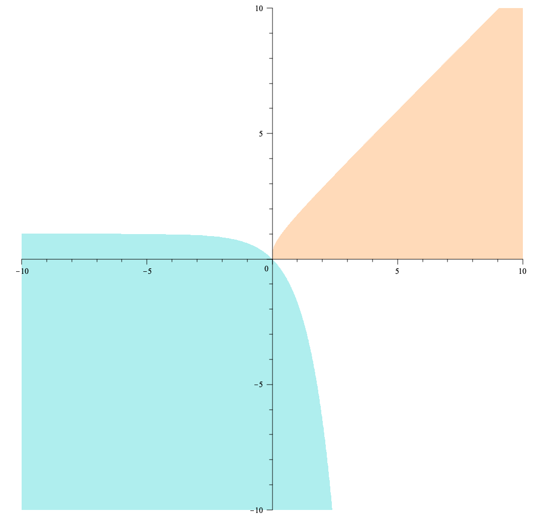
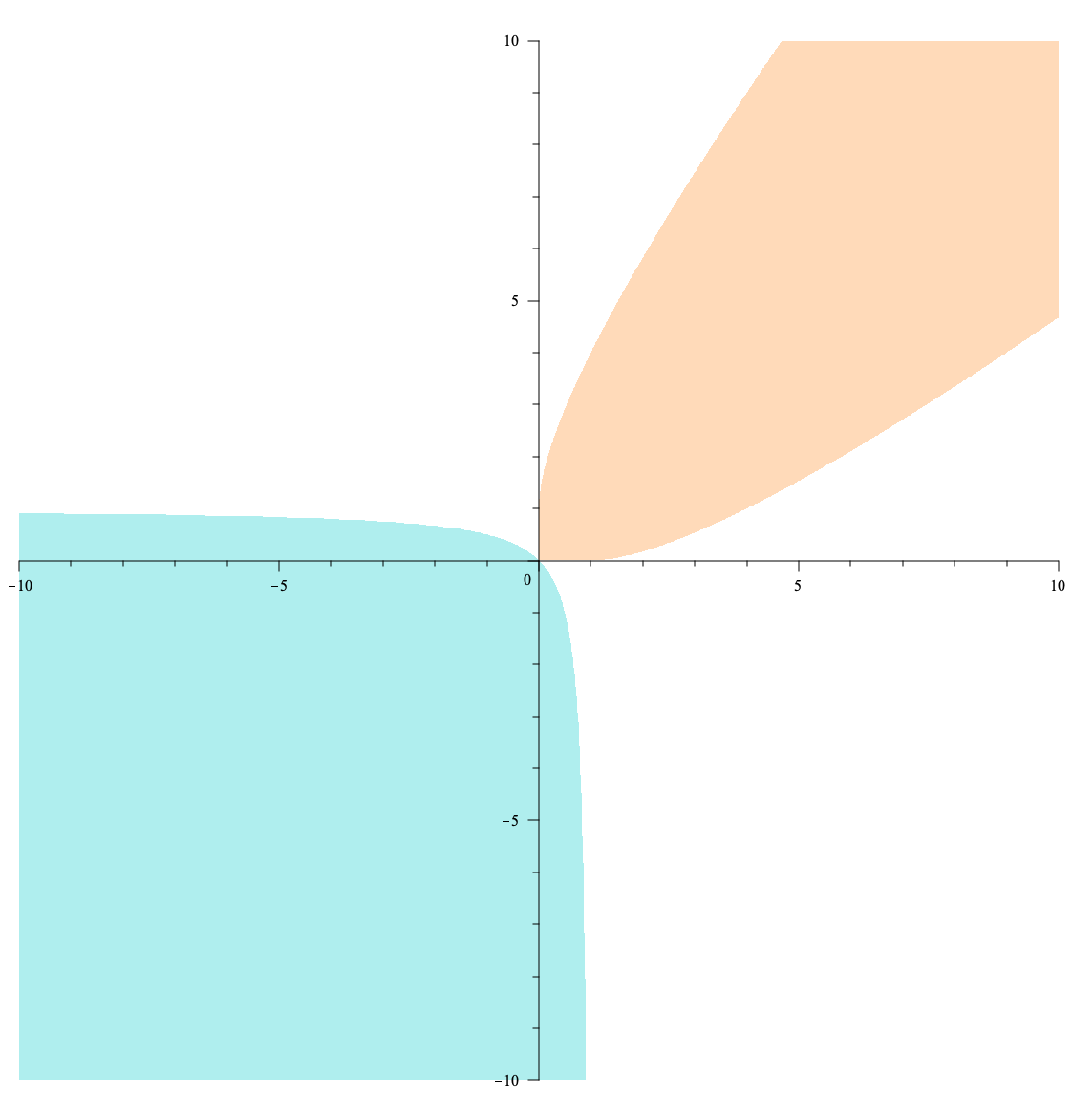
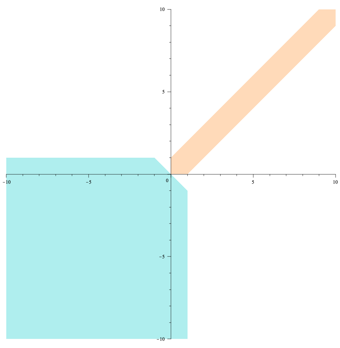
Figure 2: $D_{\varphi}$ (Turquoise) and $C_{\varphi}=(D_{\varphi})^{\circ}$ (Peach) for $\varphi_{\mathrm{KL}}$, $\varphi_{\mathrm{Hell}}$ and $\varphi_{\mathrm{Var}}$ (left to right). Since in all cases $D_{\varphi}$ and $C_{\varphi}$ are unbounded sets, we have plotted their restriction to $[-10,10]^{2}$. The purpose of including the polars $(D_{\varphi})^{\circ}$ is motivated in Appendix B .

A.2 The variational representation of $\varphi$-divergences

When $n=2$ ($Y=[2]$) we can relate $\operatorname{I}_{\mathscr{F}}$ to the Csiszár divergence $\operatorname{I}_{\varphi}$. For $\varphi\in\varPhi$ let

$${\color[rgb]{0.9,0,0}{\mathscr{F}_{\varphi}}\mathrel{\raisebox{-1.0pt}{$\overset{\textnormal{\tiny\text{def}}}{=}$}}\operatorname{\operatorname{\mathcal{L}}_{0}}(X,\operatorname{hyp}(-\varphi^{*}))}.$$ (168)

Proposition 4 and Theorem LABEL:thm:fscr_brisk_bridge immediately imply

$${\color[rgb]{0,0.88,0}\operatorname{I}_{\varphi}(E)=\operatorname{I}_{\mathscr{F}_{\varphi}}(E).}$$ (169)

It is now instructive to relate $\operatorname{I}_{\mathscr{F}_{\varphi}}(E)$ to the variational representation of $\operatorname{I}_{\varphi}$ [55], which is central to the concept of $f$-GANS [86].

Proposition 46.

Suppose $\varphi\in\varPhi$, $Y=[2]$, and $E:Y\mathrel{\rightsquigarrow}X$. Then

$${\color[rgb]{0,0.88,0}\operatorname{I}_{\mathscr{F}_{\varphi}}(E)=\sup_{g\in\operatorname{\operatorname{\mathcal{L}}_{0}}(X,\mathbb{R})}\left(\operatorname{E}_{E_{1}}g-\operatorname{E}_{E_{2}}\varphi^{*}\circ g\right).}$$ (170)

Proof.

Using (LABEL:eq:I-F-via-rho) we have

$$\operatorname{I}_{\mathscr{F}_{\varphi}}(E) =\sup_{f=(f_{1},f_{2})\in\mathscr{F}_{\varphi}}\operatorname{E}_{\rho}\left\langle\left(\frac{\mathinner{\mathrm{d}}\mathclose{}E_{1}}{\mathinner{\mathrm{d}}\mathclose{}\rho},\frac{\mathinner{\mathrm{d}}\mathclose{}E_{2}}{\mathinner{\mathrm{d}}\mathclose{}\rho}\right),(f_{1},f_{2})\right\rangle$$

$$=\sup_{\{(f_{1},f_{2})\,\mid\,f_{2}\leq-\varphi^{*}\circ f_{1}\}}\operatorname{E}_{\rho}\left\langle\left(\frac{\mathinner{\mathrm{d}}\mathclose{}E_{1}}{\mathinner{\mathrm{d}}\mathclose{}\rho},\frac{\mathinner{\mathrm{d}}\mathclose{}E_{2}}{\mathinner{\mathrm{d}}\mathclose{}\rho}\right),(f_{1},f_{2})\right\rangle$$

$$=\sup_{f_{1}\in\operatorname{\operatorname{\mathcal{L}}_{0}}(X,\mathbb{R})}\operatorname{E}_{\rho}\left\langle\left(\frac{\mathinner{\mathrm{d}}\mathclose{}E_{1}}{\mathinner{\mathrm{d}}\mathclose{}\rho},\frac{\mathinner{\mathrm{d}}\mathclose{}E_{2}}{\mathinner{\mathrm{d}}\mathclose{}\rho}\right),(f_{1},-\varphi^{*}\circ f_{1})\right\rangle,$$

since $$\frac{\mathinner{\mathrm{d}}\mathclose{}E_{2}}{\mathinner{\mathrm{d}}\mathclose{}\rho}>0 f_{2}(x)=-\varphi^{*}(f_{1}(x)) x\in X \mathscr{F}_{\varphi} \operatorname{hyp}(-\varphi^{*})$$ and we can restrict the optimization to be such that for all , and we exploited the fact that is the set of all measurable functions mapping into ,

$$=\sup_{f_{1}\in\operatorname{\operatorname{\mathcal{L}}_{0}}(X,\mathbb{R})}\operatorname{E}_{\rho}\left(\frac{\mathinner{\mathrm{d}}\mathclose{}E_{1}}{\mathinner{\mathrm{d}}\mathclose{}\rho}f_{1}-\frac{\mathinner{\mathrm{d}}\mathclose{}E_{2}}{\mathinner{\mathrm{d}}\mathclose{}\rho}\varphi^{*}\circ f_{1}\right)$$

$$=\sup_{f_{1}\in\operatorname{\operatorname{\mathcal{L}}_{0}}(X,\mathbb{R})}\int_{X}\left(f_{1}\frac{\mathinner{\mathrm{d}}\mathclose{}E_{1}}{\mathinner{\mathrm{d}}\mathclose{}\rho}-\varphi^{*}\circ f_{1}\frac{\mathinner{\mathrm{d}}\mathclose{}E_{2}}{\mathinner{\mathrm{d}}\mathclose{}\rho}\right)\mathinner{\mathrm{d}}\mathclose{}\rho$$

$$=\sup_{f_{1}\in\operatorname{\operatorname{\mathcal{L}}_{0}}(X,\mathbb{R})}\left(\int_{X}f_{1}\frac{\mathinner{\mathrm{d}}\mathclose{}E_{1}}{\mathinner{\mathrm{d}}\mathclose{}\rho}\mathinner{\mathrm{d}}\mathclose{}\rho-\int_{X}\varphi^{*}(f_{1})\frac{\mathinner{\mathrm{d}}\mathclose{}E_{2}}{\mathinner{\mathrm{d}}\mathclose{}\rho}\mathinner{\mathrm{d}}\mathclose{}\rho\right)$$

$$=\sup_{f_{1}\in\operatorname{\operatorname{\mathcal{L}}_{0}}(X,\mathbb{R})}\left(\int_{X}f_{1}\mathinner{\mathrm{d}}\mathclose{}E_{1}-\int_{X}\varphi^{*}(f_{1})\mathinner{\mathrm{d}}\mathclose{}E_{2}\right)$$

$$=\sup_{f_{1}\in\operatorname{\operatorname{\mathcal{L}}_{0}}(X,\mathbb{R})}\mathopen{}\mathclose{{}\left\lparen{\operatorname{E}_{E_{1}}f_{1}-\operatorname{E}_{E_{2}}\varphi^{*}\circ f_{1}}\right\rparen}.\qed$$

It is apparent from the proof of the above that the asymmetry in the usual variational representation (170), whereby $\varphi^{*}$ appears in only one of the terms, arises from the choice of $E_{2}$ as the dominating measure and the parametrisation of $D\in\mathfrak{D}^{2}$ by $\varphi\in\varPhi$. Such a choice is problematic if $E_{2}$ does not dominate $E_{1}$, leading to less elegant general definitions being necessary for $\operatorname{I}_{\varphi}$ [66, 65]. The one advantage of (170) over (9) when $Y=[2]$ is that the optimisation is over $\mathbb{R}$-valued functions rather than $\mathbb{R}^{2}$-valued functions. However, as seen in Section 3, the symmetric representation (9) has significant advantages in understanding the effect of the product of experiments (in the form of observation channels).

When $\varphi={\color[rgb]{0.9,0,0}{\varphi_{\mathrm{var}}}\mathrel{\raisebox{-1.0pt}{$\overset{\textnormal{\tiny\text{def}}}{=}$}}t\mapsto|t-1|}$, $\operatorname{I}_{\varphi_{\mathrm{var}}}$ is known as the variational divergence which is examined in detail in §A.3. Finally, the form of (170) suggests the variant

$$\operatorname{I}_{\mathscr{H}}(E)=\sup_{h\in\mathscr{H}}\mathopen{}\mathclose{{}\left\lparen{\operatorname{E}_{E_{1}}h-\operatorname{E}_{E_{2}}\varphi^{*}\circ h}\right\rparen},$$

where $\mathscr{H}\subsetneq\operatorname{\operatorname{\mathcal{L}}_{0}}(X,\mathbb{R})$. The functional $\operatorname{I}_{\mathscr{H}}$ is what is estimated in practice by virtue of choice of a suitable class over which to empirically optimise (170), often replacing ${E_{i}}$ by their empirical approximations ${\hat{E}_{i}^{m}}$, where for $A\in\varSigma_{X}$, ${\color[rgb]{0.9,0,0}{\hat{E}_{i}^{m}(A)}\mathrel{\raisebox{-1.0pt}{$\overset{\textnormal{\tiny\text{def}}}{=}$}}\frac{1}{m}\sum_{j\in[m]}\mathopen{}\mathclose{{}\left\llbracket{A\ni x_{j}}\right\rrbracket}}$.

An alternate way of expressing the general form of $\operatorname{I}_{\mathscr{F}}(E)$ that is similar to the classical variational representation of a binary $\varphi$-divergence is given below. Let $\mathscr{H}\subseteq\operatorname{\operatorname{\mathcal{L}}_{0}}(X,\operatorname{\mathfrak{P}}([n]))$. For $D\in\mathfrak{D}^{n}$, assume there is a measurable selection $\nabla\upsigma_{D}\in\partial\upsigma_{D}$ (confer Proposition LABEL:prop:dinf_witness). We can thus write

$$\operatorname{I}_{\nabla\upsigma_{D}\circ\mathscr{H}}(E)=\sup_{h\in\mathscr{H}}\operatorname{E}_{\rho}\ \left\langle\frac{\mathinner{\mathrm{d}}\mathclose{}E}{\mathinner{\mathrm{d}}\mathclose{}\rho},\nabla\upsigma_{D}\circ h\right\rangle.$$ (171)

Observe that $\nabla\upsigma_{D}\circ\mathscr{H}=\{\nabla\upsigma_{D}\circ h\,\mid\,h\in\mathscr{H}\}\subseteq\operatorname{\operatorname{\mathcal{L}}_{0}}(X,D)$. This is a way to use classes of functions mapping to $\mathbb{R}^{n}$ in an elegant manner to define a restricted version of $\operatorname{I}_{D}$. Observe that (171) is symmetric in the appearance of $\nabla\upsigma_{D}$, in a manner that (170) is not, but one needs to work with vector valued functions $h:X\to\mathbb{R}^{n}$. Given a function class ${\mathcal{R}}\subseteq\operatorname{\operatorname{\mathcal{L}}_{0}}(X,\mathbb{R})$, one could induce ${\color[rgb]{0.9,0,0}{\mathscr{H}_{\mathcal{R}}}\mathrel{\raisebox{-1.0pt}{$\overset{\textnormal{\tiny\text{def}}}{=}$}}\{X\ni x\mapsto(r_{1}(x),\ldots,r_{n}(x))\,\mid\,r_{i}\in{\mathcal{R}}\ \forall i\in[n]\}}$, allowing us to define ${\color[rgb]{0.9,0,0}{\operatorname{I}_{{\mathcal{R}},D}(E)}\mathrel{\raisebox{-1.0pt}{$\overset{\textnormal{\tiny\text{def}}}{=}$}}\operatorname{I}_{\nabla\upsigma_{D}\circ\mathscr{H}_{\mathcal{R}}}(E)}$.

A.3 The Variational Divergence

The binary Variational divergence has $\varphi_{\mathrm{Var}}(u)=|u-1|$ for $u\in\mathbb{R}_{\geq 0}$.

Lemma 47.

The Legendre-Fenchel conjugate of $\varphi_{\mathrm{Var}}$ is given by

$$\varphi_{\mathrm{Var}}^{*}(s)=\begin{cases}s&s\in[-1,+1]\\ +\infty&s\not\in[-1,+1].\end{cases}$$

Proof.

We have

$$\varphi_{\mathrm{Var}}^{*}(s) =\sup_{u\geq 0}u\cdot s-\varphi_{\mathrm{Var}}(u)$$

$$=\sup_{u\geq 0}u\cdot s-\begin{cases}u-1&u\geq 1\\ 1-u&u\leq 1\end{cases}$$

$$=\sup_{u\geq 0}\begin{cases}u(s-1)+1&u\geq 1\\ u(s+1)-1&u\leq 1.\end{cases}$$

Suppose $$s>1 u\geq 1 \varphi_{\mathrm{Var}}^{*}(s)=\sup_{u\geq 0}uc+1 c>0 +\infty s<-1 u\leq 1 \varphi_{\mathrm{Var}}^{*}(s)=+\infty s\in[-1,1]$$. Then the supremum is attained for and for which equals . Similarly if , the supremum is attained for and again . Suppose ; we have

$$\varphi_{\mathrm{Var}}^{*}(s) =\max\left\{\sup_{u\geq 1}u(s-1)+1,\ \sup_{u\in[0,1]}u(s+1)-1\right\}$$

$$=\max\{1(s-1)+1,\ 1(s+1)-1\}$$

$$=s\ \ \ \ \ \ \ \ \ \ \ s\in[-1,1],$$

which completes the proof. ∎

Now consider the evaluation of

$$\operatorname{I}_{{\mathscr{F}}_{\varphi_{\mathrm{Var}}}}(E) =\sup_{g:X\to\mathbb{R}}\operatorname{E}_{E_{1}}g-\operatorname{E}_{E_{2}}\varphi_{\mathrm{Var}}^{*}\circ g.$$

If, for any $$x\in X g(x)\not\in[-1,+1] -\infty g [-1,+1] E_{2}$$, , then the second term will be infinite which will push the whole value to . Thus the sup can never be attained if takes on values outside of (except on a -negligible set). Hence we need only consider

$$\operatorname{I}_{{\mathscr{F}}_{\varphi_{\mathrm{Var}}}}(E) =\sup_{g:X\to[-1,1]}\operatorname{E}_{E_{1}}g-\operatorname{E}_{E_{2}}g$$

Since the objective is linear, and the constraint set convex, the supremum is attained at the boundary and hence

$$\operatorname{I}_{{\mathscr{F}}_{\varphi_{\mathrm{Var}}}}(E) =\sup_{g:X\to\{-1,1\}}\operatorname{E}_{E_{1}}g-\operatorname{E}_{E_{2}}\varphi_{\mathrm{Var}}^{*}\circ g$$

$$=2\sup_{g:X\to\{0,1\}}\operatorname{E}_{E_{1}}g-\operatorname{E}_{E_{2}}\varphi_{\mathrm{Var}}^{*}\circ g$$ (172)

$$=2\sup_{A\in\varSigma_{X}}E_{1}(A)-E_{2}(A)$$ (173)

$$=2\sup_{A\in\varSigma_{X}}|E_{1}(A)-E_{2}(A)|,$$ (174)

where the last step is shown in [116]. Observe that (172) can also be written as

$$2\sup_{g:X\to[0,1]}\operatorname{E}_{E_{1}}g-\operatorname{E}_{E_{2}}\varphi_{\mathrm{Var}}^{*}\circ g$$ (175)

We now determine ${\color[rgb]{0.9,0,0}{{D_{\mathrm{var}}}}\mathrel{\raisebox{-1.0pt}{$\overset{\textnormal{\tiny\text{def}}}{=}$}}\operatorname{hyp}(-\varphi_{\mathrm{Var}}^{*})}$.

Lemma 48.

Let ${\color[rgb]{0.9,0,0}{H_{n,r}^{-}}\mathrel{\raisebox{-1.0pt}{$\overset{\textnormal{\tiny\text{def}}}{=}$}}\{x\in\mathbb{R}^{n}\,\mid\,\mathopen{}\mathclose{{}\left\langle{n,x}\right\rangle}-r\leq 0\}}$ denote the negative halfspace with normal vector $n$ and offset $r$. The set ${D_{\mathrm{var}}}$ can be written

$${D_{\mathrm{var}}}=H_{1_{2},0}^{-}\cap H_{\mathrm{e}_{1},1}^{-}\cap H_{\mathrm{e}_{2},1}^{-}.$$ (176)

Proof.

We have

$$\operatorname{hyp}(-\varphi_{\mathrm{Var}}^{*}) =\mathopen{}\mathclose{{}\left\{{(x,y)\in\mathbb{R}^{2}}\mathrel{}\middle|\mathrel{}{y\leq-\varphi_{\mathrm{Var}}^{*}(x)}\right\}}$$

$$=\left\{(x,y)\in\mathbb{R}^{2}\,\mid\,y\leq\begin{cases}-x&x\in[-1,+1]\\ -\infty&x\not\in[-1,+1]\end{cases}\right\}$$

$$=\mathopen{}\mathclose{{}\left\{{(x,y)\in\mathbb{R}^{2}}\mathrel{}\middle|\mathrel{}{x\in[-1,+1],y\leq-x}\right\}}.$$

Now Lemma LABEL:lem:dinf_conv_closure implies $\operatorname{I}_{D}(E)=\operatorname{I}_{\operatorname{co}D}(E)$, and hence we can take the convex hull of the above to obtain

$${D_{\mathrm{var}}} =\mathopen{}\mathclose{{}\left\{{(x,y)\in\mathbb{R}^{2}}\mathrel{}\middle|\mathrel{}{y\leq 1}\right\}}\cap\{(x,y)\in\mathbb{R}^{2}\,\mid\,y\leq-x\}\cap\mathopen{}\mathclose{{}\left\{{(x,y)\in\mathbb{R}^{2}}\mathrel{}\middle|\mathrel{}{x\leq 1}\right\}}$$

$$=\{(x,y)\in\mathbb{R}^{2}\,\mid\,y\leq 1\mbox{\ and\ }x\leq 1\mbox{\ and\ }y\leq-x\}.$$

We can thus more compactly write ${D_{\mathrm{var}}}$ as in (176). ∎

Lemma 48 suggests the following generalisation which we now take as a definition

$${\color[rgb]{0.9,0,0}{{D_{\mathrm{var}}^{(n)}}}}\mathrel{\raisebox{-1.0pt}{$\overset{\textnormal{\tiny\text{def}}}{=}$}}H_{1_{n},0}^{-}\cap\bigcap_{i\in[n]}H_{\mathrm{e}_{i},1}^{-}.$$ (177)

Observe that ${D_{\mathrm{var}}^{(n)}}$ is the maximal (by set inclusion) element of $\operatorname{\mathcaleu{D}}(\mathbb{R}^{n},\mathbb{R}_{\leq 0}^{n})$ satisfying the normalisation condition $\bigvee_{i\in[n]}\upsigma_{D}(\mathrm{e}_{i})=1$. We now compute $\upsigma_{{D_{\mathrm{var}}^{(n)}}}$.

Lemma 49.

The support function of ${D_{\mathrm{var}}^{(n)}}$ is given by

$$\upsigma_{{D_{\mathrm{var}}^{(n)}}}(x)=\sum_{i\in[n]}x_{i}-n\bigwedge_{j\in[n]}x_{j}.$$

Proof.

Note that ${D_{\mathrm{var}}^{(n)}}$ is a intersection of half spaces and thus its support function is the same as the support function of its extreme points, which is the union of the $n$ vertices created. Denote the vertices $v_{j}$ for $j\in[n]$. We have

$$v_{j} =H_{1_{n},0}^{-}\cap\bigcap_{i\in[n]\setminus\{j\}}H_{\mathrm{e}_{i},1}^{-}$$

$$=\{x\in\mathbb{R}^{n}\,\mid\,\mathopen{}\mathclose{{}\left\langle{x,\,\mathrm{e}_{i}}\right\rangle}-1=0\ \forall i\neq j\mbox{\ and\ }\mathopen{}\mathclose{{}\left\langle{x,\,1_{n}}\right\rangle}=0\}$$

$$=\left\{x\in\mathbb{R}^{n}\,\mid\,x_{i}=i\ \forall i\neq j\mbox{\ and\ }\textstyle\sum_{k\in[n]}x_{k}=0\right\}$$

$$=\{x\in\mathbb{R}^{n}\,\mid\,x_{i}=1\ \forall i\neq j\mbox{\ and\ }x_{j}=-(n-1)\}$$

$$=1_{n}-n\mathrm{e}_{j}.$$ (178)

Thus for $x\in\mathbb{R}_{\geq 0}^{n}$, using [50, Theorem C.3.3.2 (ii)] we have $\upsigma_{\operatorname{\overline{\operatorname{co}}}(\cup_{j\in[n]}\{v_{j}\}}=\sup_{j\in[n]}\upsigma_{\{v_{j}\})}$ and hence

$$\upsigma_{D_{\mathrm{var}}^{(n)}}(x) =\sup_{j\in[n]}\langle 1_{n}-n\mathrm{e}_{j},\,x\rangle$$

$$=\mathopen{}\mathclose{{}\left\langle{1_{n},\,x}\right\rangle}+n\sup_{j\in[n]}-x_{j}$$

$$=\sum_{i\in[n]}x_{i}-n\bigwedge_{j\in[n]}x_{j}.\qed$$

We can now determine an explicit expression for $\operatorname{I}_{D_{\mathrm{var}}^{(n)}}(E)$. Let $(\bar{X}_{1},\ldots,\bar{X}_{n})$ be a measurable partition of $X$ (i.e. $\bar{X}_{i}$ are measurable for $i\in[n]$) defined via

$${\color[rgb]{0.9,0,0}{\bar{X}_{i}}\mathrel{\raisebox{-1.0pt}{$\overset{\textnormal{\tiny\text{def}}}{=}$}}\left\{x\in X\,\mid\,\textstyle\min\left(\operatornamewithlimits{Argmin}_{j\in[n]}\frac{\mathinner{\mathrm{d}}\mathclose{}\,E_{j}}{\mathinner{\mathrm{d}}\mathclose{}\,\rho}(x)=i\right)\right\}}.$$ (179)

(The additional $\min$ is to break ties.) It is immediate that this is indeed a partition of $X$, i.e. $\bigcup_{k\in[n]}\bar{X}_{k}=X$ and $\bar{X}_{i}\cap\bar{X}_{j}=\varnothing$ for $i\neq j$. Consequently

$$\operatorname{I}_{D_{\mathrm{var}}^{(n)}}(E) =\int_{X}\sum_{i\in[n]}\frac{\mathinner{\mathrm{d}}\mathclose{}E_{i}}{\mathinner{\mathrm{d}}\mathclose{}\rho}(x)\rho(\mathinner{\mathrm{d}}\mathclose{}x)-n\int_{X}\bigwedge_{j\in[n]}\frac{\mathinner{\mathrm{d}}\mathclose{}E_{j}}{\mathinner{\mathrm{d}}\mathclose{}\rho}(x)\rho(\mathinner{\mathrm{d}}\mathclose{}x)$$

$$=\sum_{i\in[n]}\int_{X}\mathinner{\mathrm{d}}\mathclose{}E_{i}-n\int_{X}\bigwedge_{j\in[n]}\frac{\mathinner{\mathrm{d}}\mathclose{}E_{j}}{\mathinner{\mathrm{d}}\mathclose{}\rho}(x)\rho(\mathinner{\mathrm{d}}\mathclose{}x)$$ (180)

$$=n\left[1-\sum_{k\in[n]}\int_{\bar{X}_{k}}\frac{\mathinner{\mathrm{d}}\mathclose{}E_{k}}{\mathinner{\mathrm{d}}\mathclose{}\rho}(x)\rho(\mathinner{\mathrm{d}}\mathclose{}x)\right]$$

$$=n\left[1-\sum_{k\in[n]}E_{k}(\bar{X}_{k})\right],$$

using the properties of the partition $$(\bar{X}_{1},\ldots,\bar{X}_{n})$$.

Observe that choosing any other partition of $X$ would result in a larger value of the second integral in (180) and thus a smaller value for the overall expression. Thus if ${\mathcal{P}}_{n}(X)$ denotes the set of all measurable $n$-partitions of $X$, we can write

$$\operatorname{I}_{D_{\mathrm{var}}^{(n)}}(E)=\sup_{(X_{1},\ldots,X_{m})\in{\mathcal{P}}_{n}(X)}n\left[1-\sum_{k\in[n]}E_{k}(X_{k})\right].$$ (182)

When $Y=[2]$, we obtain

$$\operatorname{I}_{D_{\mathrm{var}}^{(2)}}(E) =\sup_{(X_{1},X_{2})\in{\mathcal{P}}_{2}(X)}2[1-(E_{1}(X_{1})+E_{2}(X_{2}))]$$

$$=2\sup_{\begin{subarray}{c}X_{1}\subseteq X\\ X_{1}\ \mathrm{measurable}\end{subarray}}[1-(E_{1}(X_{1})+E_{2}(X\setminus X_{1}))]$$

$$=2\sup_{\begin{subarray}{c}X_{1}\subseteq X\\ X_{1}\ \mathrm{measurable}\end{subarray}}[1-(E_{1}(X_{1})+1-E_{2}(X_{1}))]$$

$$=2\sup_{\begin{subarray}{c}X_{1}\subseteq X\\ X_{1}\ \mathrm{measurable}\end{subarray}}[E_{1}(X_{1})-E_{2}(X_{1})],$$

which can be recognised as being equivalent to (173).

Finally we observe a special case of (LABEL:eq:IDSE) for $D={D_{\mathrm{var}}^{(n)}}$ when $S$ takes the particular symmetric form $S_{\alpha}$ where the $j$th column of $S_{\alpha}^{*}$ is $s_{j}^{*}=\alpha\mathrm{e}_{j}+\frac{1-\alpha}{n}1_{n}$. When $\alpha=1$ this is the identity matrix, and for $\alpha\in[0,1]$ it corresponds to the observation channel providing the correct label with probability $\alpha$ and with probability $1-\alpha$ a label chosen at random from $[n]$ is chosen (which could in fact be correct). The set $S_{\alpha}^{*}{D_{\mathrm{var}}^{(n)}}$ can be readily determined by exploiting the fact we need only determine its support function $\upsigma_{S_{\alpha}^{*}{D_{\mathrm{var}}^{(n)}}}(x)$ for $x\in\mathbb{R}_{\geq 0}^{n}$. Thus we can exploit (178) and we need only compute (for $j\in[n]$)

$$S_{\alpha}^{*}v_{j} =1_{n}-n\left(\alpha\mathrm{e}_{j}+\frac{1-\alpha}{n}1_{n}\right)$$

$$=\alpha(1_{n}-n\mathrm{e}_{j})$$

$$=\alpha v_{j}.$$

Thus $\upsigma_{S_{\alpha}^{*}{D_{\mathrm{var}}^{(n)}}}=\alpha\upsigma_{D}$ and so for any $\alpha\in[0,1]$ and any $n$, we have the homogeneous relationship

$${\color[rgb]{0,0.88,0}\operatorname{I}_{D_{\mathrm{var}}^{(n)}}(S_{\alpha}E)=\alpha\operatorname{I}_{D_{\mathrm{var}}^{(n)}}(E),}$$

which we note has the same measure of information on either side of the equality (analogous to the typical strong data processing inequalities one finds in the literature).

B $D$-Information as an Expected Gauge Function

Classical binary information “divergences” are sometimes supposed to be “like” a distance (a metric). In this appendix we show that there is an element of truth in this supposition. Metrics (as a formal notion of “distance”) are often (not always) induced by norms, and norms are particular examples of convex gauge functions (Minkowski functionals). In this appendix we show that it follows almost immediately from our definition of $D$-information that it is indeed an expected gauge function, albeit one where the associated “unit ball” of the gauge is neither symmetric nor compact. The restriction of $D\in\mathfrak{D}$ allows an insightful representation of $\operatorname{I}_{D}$ making use of the classical polar duality of closed convex sets containing the origin.

The conic hull of a set $C\subset\mathbb{R}^{n}$ is ${\color[rgb]{0.9,0,0}{\operatorname{pos}C}\mathrel{\raisebox{-1.0pt}{$\overset{\textnormal{\tiny\text{def}}}{=}$}}(0,\infty)\cdot C}$. Given $C\in\operatorname{\mathcaleu{K}}(\mathbb{R}^{n})$, the polar of $C$ is defined by

$${\color[rgb]{0.9,0,0}{C^{\circ}}\mathrel{\raisebox{-1.0pt}{$\overset{\textnormal{\tiny\text{def}}}{=}$}}\{x^{*}\,\mid\,\forall x\in C,\ \langle x,x^{*}\rangle\leq 1\}}.$$

We will make use of the following from [100, Theorem 14.6]:

Proposition 50.

Suppose $C,C^{\circ}\in\operatorname{\mathcaleu{K}}(\mathbb{R}^{n})$ are a polar pair both containing the origin. Then $(\operatorname{rec}C)^{\circ}=\operatorname{cl}\operatorname{pos}C^{\circ}$.

Given $C\in\operatorname{\mathcaleu{K}}(\mathbb{R}^{n})$, the gauge of $C$ is defined by

$${\color[rgb]{0.9,0,0}{\gamma_{C}(x)}\mathrel{\raisebox{-1.0pt}{$\overset{\textnormal{\tiny\text{def}}}{=}$}}\inf\{\mu\geq 0\,\mid\,x\in\mu C\}}.$$

Obviously given the gauge $\gamma_{C}$ one can recover $C$ via $C=\operatorname{lev}_{\leq 1}\gamma_{C}=\{x\,\mid\,\gamma_{C}(x)\leq 1\}.$ (If $C$ is symmetric about the origin, then $\gamma_{C}$ is a norm.) Let

$${\color[rgb]{0.9,0,0}{\mathfrak{C}_{0}^{n}}\mathrel{\raisebox{-1.0pt}{$\overset{\textnormal{\tiny\text{def}}}{=}$}}\left\{C\in\operatorname{\mathcaleu{K}}(\mathbb{R}^{n})\,\mid\,\operatorname{pos}C\subseteq\mathbb{R}_{\geq 0}^{n},\ 0\in\operatorname{bd}C,\ \operatorname{pos}1_{n}\subseteq C\right\}}.$$

Lemma 51.

If $D\in\mathfrak{D}_{0}^{n}$ then $D^{\circ}\in\mathfrak{C}_{0}^{n}$.

Proof.

If $D$ is convex then so is $D^{\circ}$. By Proposition 50, since $0\in D$, $\operatorname{rec}D$ is the largest cone contained in $D$ and $(\operatorname{rec}D)^{\circ}=\operatorname{cl}\operatorname{pos}C$ is the smallest cone containing $C$. Thus when $\operatorname{rec}D=\{x\in\mathbb{R}^{n}\,\mid\,\langle x,1_{n}\rangle\leq 1\}$, $\operatorname{cl}\operatorname{pos}C=\{\alpha 1_{n}\,\mid\,\alpha\geq 0\}$. Regardless of the choice of $D$, we always have $0\in\operatorname{bd}D^{\circ}$. The final condition in the definition of $\mathfrak{C}_{0}^{n}$ follows since $D\subseteq C\Rightarrow D^{\circ}\supseteq C^{\circ}$, and $(\operatorname{lev}_{\leq 0}\langle,\cdot,1_{n}\rangle)^{\circ}=\operatorname{pos}1_{n}$. ∎

Gauges and support functions are dual to each other in the polar sense [50, Corollary C.3.2.5]:

Lemma 52.

Suppose $C\in\operatorname{\mathcaleu{K}}(\mathbb{R}^{n})$, then $\sigma_{C}=\gamma_{C^{\circ}}$.

Proposition 53.

For any $D\in\mathfrak{D}^{n}$, $D^{\circ}\in\mathfrak{C}^{n}$ and for any $E\colon[n]\mathrel{\rightsquigarrow}X$, and any reference measure $\rho$,

$${\color[rgb]{0,0.88,0}\operatorname{I}_{D}(E)=\int_{X}\gamma_{D^{\circ}}\left(\textstyle\frac{\mathinner{\mathrm{d}}\mathclose{}E}{\mathinner{\mathrm{d}}\mathclose{}\rho}\right)\mathinner{\mathrm{d}}\mathclose{}\rho.}$$ (183)

Proof.

The first claim is just lemma 51. The second claim follows by applying Lemma 52 pointwise. ∎

Expressing $\operatorname{I}_{D}$ as an average of a gauge function as in (183) justifies the oft made claim that divergence are “like” distances in some sense; the fact that $D^{\circ}$ is not symmetric is why it is merely “like”. One can see that $\operatorname{I}_{D}$ is “gauging” the average degree to which the vector $\frac{\mathinner{\mathrm{d}}\mathclose{}E}{\mathinner{\mathrm{d}}\mathclose{}\rho}(x)$ is “close” to one of the canonical basis vectors $e_{i}$, $i\in[n]$ since for $D^{\circ}\in\mathfrak{C}_{0}^{n}$, $\gamma_{D^{\circ}}(e_{i})>0$ in that case. Conversely, since $\operatorname{cl}\operatorname{pos}D^{\circ}=\{\alpha 1_{n}\,\mid\,\alpha\geq 0\}$, we always have $\gamma_{D^{\circ}}(1_{n})=\sigma_{D}(1_{n})=0$, corresponding to situations where $\frac{\mathinner{\mathrm{d}}\mathclose{}E}{\mathinner{\mathrm{d}}\mathclose{}\rho}(x)=1_{n}$, and consequently it being impossible to distinguish between the outcomes of the experiment at that $x$ — in other words a complete absence of “information.” Some example of polars of $D$ illustrated in Figure 3.

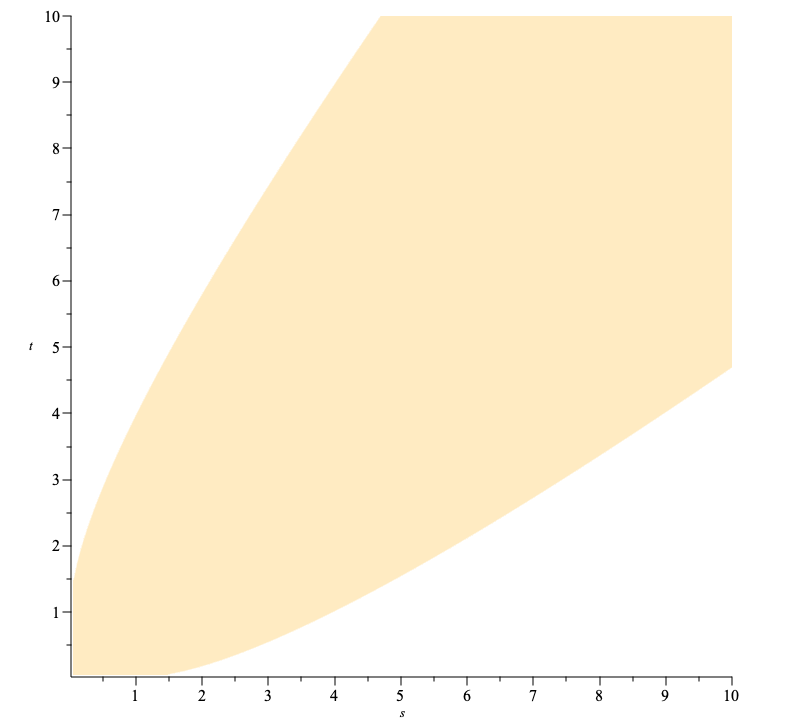
Figure 3: The corresponding polars for $R_{r}D_{\mathrm{Hell}}$ for $r=1,0.8,0.6$ (restricted to $[0,10]^{2}$) corresponding to the set-up as in Figure LABEL:fig:C-D-r. Observe that for any $E\colon[2]\mathrel{\rightsquigarrow}X$, as $r\downarrow 0.5$, the composition $R_{r}E$ approaches the totally non-informative experiment $E^{\mathrm{tni}}$, and $\operatorname{I}_{R_{r}^{*}D}$ approaches what we might (oxymoronically) call the totally noninformative information measure $\operatorname{I}^{\mathrm{tni}}=\operatorname{I}_{D_{\mathrm{tni}}}$, where $D_{\mathrm{tni}}=\{x\in\mathbb{R}^{n}\,\mid\,\langle x,1_{n}\rangle\leq 0\}$ and $C_{\mathrm{tni}}=D_{\mathrm{tni}}^{\circ}=\{\alpha 1_{n}\,\mid\,\alpha\geq 0\}$. The name is justified since $\operatorname{I}^{\mathrm{tni}}(E)=0$ for all experiments $E$.

C Unconstrained and Constrained Entropies

Historically, the notion of the entropy of a single distribution (or random variable) preceded measures of information between two or more distributions (or random variables). There is a large literature on different notions of entropy, starting with [109], with $\varphi$-entropies (analogous to $\varphi$-divergences) specifically considered in [28, 29, 13]. In this appendix we recall how the entropy of a distribution $\mu\in\operatorname{\mathfrak{P}}(X)$ can be defined on the basis of comparison against a “uniform” measure $\upsilon\in\operatorname{\mathfrak{P}}(X)$ cf. [119, 82]. Traditionally this comparison measure is taken for granted as being Lebesgue measure, but we shall see it is an arbitrary choice and the choice matters.

Given $\mu\in\operatorname{\mathfrak{P}}(X)$, define the experiment $E_{\mu}^{\upsilon}:[2]\mathrel{\rightsquigarrow}X$ via

$${\color[rgb]{0.9,0,0}{E_{\mu}^{\upsilon}(1,\cdot)}\mathrel{\raisebox{-1.0pt}{$\overset{\textnormal{\tiny\text{def}}}{=}$}}\mu(\cdot)}\mbox{\ \ \ and\ \ \ }{\color[rgb]{0.9,0,0}{E_{\mu}^{\upsilon}(2,\cdot)}\mathrel{\raisebox{-1.0pt}{$\overset{\textnormal{\tiny\text{def}}}{=}$}}\upsilon(\cdot)}.$$ (184)

The measure $\mu$ is that which we are interested in (we wish to compute its “entropy”); the measure $\upsilon$ is a choice we make regarding what to compare it against. Often $\upsilon=\lambda$, Lebesgue measure. The unconstrained entropy can be defined as follows. For $D\in\operatorname{\mathcaleu{D}}(\mathbb{R}^{2},\mathbb{R}_{\leq 0}^{2})$, the $D$-entropy of $\mu$ relative to $\upsilon$ is

$${\color[rgb]{0.9,0,0}{\operatorname{H}_{D}^{\upsilon}(\mu)}\mathrel{\raisebox{-1.0pt}{$\overset{\textnormal{\tiny\text{def}}}{=}$}}\operatorname{I}_{D}(E_{\mu}^{\upsilon})}.$$ (185)

Define $D_{\varphi}$ via (16) and write ${\color[rgb]{0.9,0,0}{\operatorname{H}^{\upsilon}_{\varphi}(\mu)}\mathrel{\raisebox{-1.0pt}{$\overset{\textnormal{\tiny\text{def}}}{=}$}}\operatorname{H}_{D_{\varphi}}^{\upsilon}(\mu)}$, the usual definition of $\varphi$-entropy when $\upsilon$ is chosen to be “uniform” over the support of $\mu$. Choose $\rho$ as usual to be absolutely continuous with respect to $\mu$ and $\upsilon$. Then using Proposition LABEL:prop:dinf_support_representation we have $\operatorname{H}_{\varphi}^{\upsilon}(\mu)=\int_{X}\upsigma_{D_{\varphi}}\left(\mathinner{\mathchoice{\frac{\mathinner{\mathrm{d}}\mathclose{}\mu}{\mathinner{\mathrm{d}}\mathclose{}\rho}}{\raisebox{2.15277pt}{$\scriptstyle\mathinner{\mathrm{d}}\mathclose{}\mu$}\mkern-3.0mu/\mkern-3.0mu\raisebox{-2.15277pt}{$\scriptstyle\mathinner{\mathrm{d}}\mathclose{}\rho$}}{\raisebox{1.29167pt}{$\scriptscriptstyle\mathinner{\mathrm{d}}\mathclose{}\mu$}\scriptstyle{\mkern-3.0mu/\mkern-3.0mu}\raisebox{-0.90417pt}{$\scriptscriptstyle\mathinner{\mathrm{d}}\mathclose{}\rho$}}{\raisebox{1.29167pt}{$\scriptscriptstyle\mathinner{\mathrm{d}}\mathclose{}\mu$}\scriptstyle{\mkern-3.0mu/\mkern-3.0mu}\raisebox{-0.90417pt}{$\scriptscriptstyle\mathinner{\mathrm{d}}\mathclose{}\rho$}}},\mathinner{\mathchoice{\frac{\mathinner{\mathrm{d}}\mathclose{}\upsilon}{\mathinner{\mathrm{d}}\mathclose{}\rho}}{\raisebox{2.15277pt}{$\scriptstyle\mathinner{\mathrm{d}}\mathclose{}\upsilon$}\mkern-3.0mu/\mkern-3.0mu\raisebox{-2.15277pt}{$\scriptstyle\mathinner{\mathrm{d}}\mathclose{}\rho$}}{\raisebox{1.29167pt}{$\scriptscriptstyle\mathinner{\mathrm{d}}\mathclose{}\upsilon$}\scriptstyle{\mkern-3.0mu/\mkern-3.0mu}\raisebox{-0.90417pt}{$\scriptscriptstyle\mathinner{\mathrm{d}}\mathclose{}\rho$}}{\raisebox{1.29167pt}{$\scriptscriptstyle\mathinner{\mathrm{d}}\mathclose{}\upsilon$}\scriptstyle{\mkern-3.0mu/\mkern-3.0mu}\raisebox{-0.90417pt}{$\scriptscriptstyle\mathinner{\mathrm{d}}\mathclose{}\rho$}}}\right)\mathinner{\mathrm{d}}\mathclose{}\rho=\int_{X}\breve{\varphi}\left(\mathinner{\mathchoice{\frac{\mathinner{\mathrm{d}}\mathclose{}\mu}{\mathinner{\mathrm{d}}\mathclose{}\rho}}{\raisebox{2.15277pt}{$\scriptstyle\mathinner{\mathrm{d}}\mathclose{}\mu$}\mkern-3.0mu/\mkern-3.0mu\raisebox{-2.15277pt}{$\scriptstyle\mathinner{\mathrm{d}}\mathclose{}\rho$}}{\raisebox{1.29167pt}{$\scriptscriptstyle\mathinner{\mathrm{d}}\mathclose{}\mu$}\scriptstyle{\mkern-3.0mu/\mkern-3.0mu}\raisebox{-0.90417pt}{$\scriptscriptstyle\mathinner{\mathrm{d}}\mathclose{}\rho$}}{\raisebox{1.29167pt}{$\scriptscriptstyle\mathinner{\mathrm{d}}\mathclose{}\mu$}\scriptstyle{\mkern-3.0mu/\mkern-3.0mu}\raisebox{-0.90417pt}{$\scriptscriptstyle\mathinner{\mathrm{d}}\mathclose{}\rho$}}},\mathinner{\mathchoice{\frac{\mathinner{\mathrm{d}}\mathclose{}\upsilon}{\mathinner{\mathrm{d}}\mathclose{}\rho}}{\raisebox{2.15277pt}{$\scriptstyle\mathinner{\mathrm{d}}\mathclose{}\upsilon$}\mkern-3.0mu/\mkern-3.0mu\raisebox{-2.15277pt}{$\scriptstyle\mathinner{\mathrm{d}}\mathclose{}\rho$}}{\raisebox{1.29167pt}{$\scriptscriptstyle\mathinner{\mathrm{d}}\mathclose{}\upsilon$}\scriptstyle{\mkern-3.0mu/\mkern-3.0mu}\raisebox{-0.90417pt}{$\scriptscriptstyle\mathinner{\mathrm{d}}\mathclose{}\rho$}}{\raisebox{1.29167pt}{$\scriptscriptstyle\mathinner{\mathrm{d}}\mathclose{}\upsilon$}\scriptstyle{\mkern-3.0mu/\mkern-3.0mu}\raisebox{-0.90417pt}{$\scriptscriptstyle\mathinner{\mathrm{d}}\mathclose{}\rho$}}}\right)\mathinner{\mathrm{d}}\mathclose{}\rho=\int_{X}\mathinner{\mathchoice{\frac{\mathinner{\mathrm{d}}\mathclose{}\mu}{\mathinner{\mathrm{d}}\mathclose{}\rho}}{\raisebox{2.15277pt}{$\scriptstyle\mathinner{\mathrm{d}}\mathclose{}\mu$}\mkern-3.0mu/\mkern-3.0mu\raisebox{-2.15277pt}{$\scriptstyle\mathinner{\mathrm{d}}\mathclose{}\rho$}}{\raisebox{1.29167pt}{$\scriptscriptstyle\mathinner{\mathrm{d}}\mathclose{}\mu$}\scriptstyle{\mkern-3.0mu/\mkern-3.0mu}\raisebox{-0.90417pt}{$\scriptscriptstyle\mathinner{\mathrm{d}}\mathclose{}\rho$}}{\raisebox{1.29167pt}{$\scriptscriptstyle\mathinner{\mathrm{d}}\mathclose{}\mu$}\scriptstyle{\mkern-3.0mu/\mkern-3.0mu}\raisebox{-0.90417pt}{$\scriptscriptstyle\mathinner{\mathrm{d}}\mathclose{}\rho$}}}\varphi\mathopen{}\mathclose{{}\left\lparen{\mathinner{\mathchoice{\frac{\mathinner{\mathrm{d}}\mathclose{}\mu}{\mathinner{\mathrm{d}}\mathclose{}\rho}}{\raisebox{2.15277pt}{$\scriptstyle\mathinner{\mathrm{d}}\mathclose{}\mu$}\mkern-3.0mu/\mkern-3.0mu\raisebox{-2.15277pt}{$\scriptstyle\mathinner{\mathrm{d}}\mathclose{}\rho$}}{\raisebox{1.29167pt}{$\scriptscriptstyle\mathinner{\mathrm{d}}\mathclose{}\mu$}\scriptstyle{\mkern-3.0mu/\mkern-3.0mu}\raisebox{-0.90417pt}{$\scriptscriptstyle\mathinner{\mathrm{d}}\mathclose{}\rho$}}{\raisebox{1.29167pt}{$\scriptscriptstyle\mathinner{\mathrm{d}}\mathclose{}\mu$}\scriptstyle{\mkern-3.0mu/\mkern-3.0mu}\raisebox{-0.90417pt}{$\scriptscriptstyle\mathinner{\mathrm{d}}\mathclose{}\rho$}}}\mathinner{\mathchoice{\frac{\mathinner{\mathrm{d}}\mathclose{}\rho}{\mathinner{\mathrm{d}}\mathclose{}\upsilon}}{\raisebox{2.15277pt}{$\scriptstyle\mathinner{\mathrm{d}}\mathclose{}\rho$}\mkern-3.0mu/\mkern-3.0mu\raisebox{-2.15277pt}{$\scriptstyle\mathinner{\mathrm{d}}\mathclose{}\upsilon$}}{\raisebox{1.29167pt}{$\scriptscriptstyle\mathinner{\mathrm{d}}\mathclose{}\rho$}\scriptstyle{\mkern-3.0mu/\mkern-3.0mu}\raisebox{-0.90417pt}{$\scriptscriptstyle\mathinner{\mathrm{d}}\mathclose{}\upsilon$}}{\raisebox{1.29167pt}{$\scriptscriptstyle\mathinner{\mathrm{d}}\mathclose{}\rho$}\scriptstyle{\mkern-3.0mu/\mkern-3.0mu}\raisebox{-0.90417pt}{$\scriptscriptstyle\mathinner{\mathrm{d}}\mathclose{}\upsilon$}}}}\right\rparen}\mathinner{\mathrm{d}}\mathclose{}\rho=\int_{X}\varphi\mathopen{}\mathclose{{}\left\lparen{\mathinner{\mathchoice{\frac{\mathinner{\mathrm{d}}\mathclose{}\mu}{\mathinner{\mathrm{d}}\mathclose{}\upsilon}}{\raisebox{2.15277pt}{$\scriptstyle\mathinner{\mathrm{d}}\mathclose{}\mu$}\mkern-3.0mu/\mkern-3.0mu\raisebox{-2.15277pt}{$\scriptstyle\mathinner{\mathrm{d}}\mathclose{}\upsilon$}}{\raisebox{1.29167pt}{$\scriptscriptstyle\mathinner{\mathrm{d}}\mathclose{}\mu$}\scriptstyle{\mkern-3.0mu/\mkern-3.0mu}\raisebox{-0.90417pt}{$\scriptscriptstyle\mathinner{\mathrm{d}}\mathclose{}\upsilon$}}{\raisebox{1.29167pt}{$\scriptscriptstyle\mathinner{\mathrm{d}}\mathclose{}\mu$}\scriptstyle{\mkern-3.0mu/\mkern-3.0mu}\raisebox{-0.90417pt}{$\scriptscriptstyle\mathinner{\mathrm{d}}\mathclose{}\upsilon$}}}}\right\rparen}\mathinner{\mathrm{d}}\mathclose{}\mu=\operatorname{E}_{\mu}\varphi\mathopen{}\mathclose{{}\left\lparen{\mathinner{\mathchoice{\frac{\mathinner{\mathrm{d}}\mathclose{}\mu}{\mathinner{\mathrm{d}}\mathclose{}\upsilon}}{\raisebox{2.15277pt}{$\scriptstyle\mathinner{\mathrm{d}}\mathclose{}\mu$}\mkern-3.0mu/\mkern-3.0mu\raisebox{-2.15277pt}{$\scriptstyle\mathinner{\mathrm{d}}\mathclose{}\upsilon$}}{\raisebox{1.29167pt}{$\scriptscriptstyle\mathinner{\mathrm{d}}\mathclose{}\mu$}\scriptstyle{\mkern-3.0mu/\mkern-3.0mu}\raisebox{-0.90417pt}{$\scriptscriptstyle\mathinner{\mathrm{d}}\mathclose{}\upsilon$}}{\raisebox{1.29167pt}{$\scriptscriptstyle\mathinner{\mathrm{d}}\mathclose{}\mu$}\scriptstyle{\mkern-3.0mu/\mkern-3.0mu}\raisebox{-0.90417pt}{$\scriptscriptstyle\mathinner{\mathrm{d}}\mathclose{}\upsilon$}}}}\right\rparen}$. As usual, the choice of reference measure $\rho$ does not matter. But the choice of comparison measure $\upsilon$ does matter since $\operatorname{H}_{\varphi}^{\upsilon}(\mu)=\operatorname{I}_{\varphi}(E_{\mu}^{\upsilon})$ which clearly depends upon the choice of $\upsilon$.

This perspective offers an insight into why the entropy is difficult to estimate: one is implicitly attempting to determine the Bayes risk for a statistical decision problem where the two class conditional distributions are the given $\mu$ and the reference (uniform) measure $\upsilon$ using a loss $\ell$ induced by $\varphi$ as in Remark LABEL:rem:bridge-n-2. This insight also offers an effective approach to estimating the entropy as we now explain.

The constrained entropy of $\mu$ relative to $\upsilon$ is defined similarly,

$${\color[rgb]{0.9,0,0}{\operatorname{H}_{\mathscr{F}}^{\upsilon}(\mu)}\mathrel{\raisebox{-1.0pt}{$\overset{\textnormal{\tiny\text{def}}}{=}$}}\operatorname{I}_{\mathscr{F}}(E_{\mu}^{\upsilon})},$$ (186)

and simply amounts to regularising the $\varphi$-entropy (where $\mathscr{F}(X)\subseteq D_{\varphi}$). This immediately suggests ways to estimate the entropy of a random variable defined on $X$ (especially when $X$ is high dimensional): use the bridge between $\mathscr{F}$-information and the $\mathscr{H}$-constrained Bayes risk and simply exploit the wide range of extant methods for solving binary class-probability estimation problems. That is given a random sample $\{x_{1},\ldots,x_{m}\}$ drawn iid from $\mu$, estimate the entropy from the empirical measure ${\color[rgb]{0.9,0,0}{\mu^{m}(A)}\mathrel{\raisebox{-1.0pt}{$\overset{\textnormal{\tiny\text{def}}}{=}$}}\frac{1}{m}\sum_{i\in[m]}\mathopen{}\mathclose{{}\left\llbracket{x_{i}\in A}\right\rrbracket}}$ via $\operatorname{H}_{\mathscr{F}}^{\upsilon}(\mu^{m})=\operatorname{I}_{\mathscr{F}}(\mu^{m},\upsilon)$. The estimate is regularised by the choice of $\mathscr{F}$. Observe that one can immediately define a generalised mutual information using $\operatorname{I}_{\mathcal{F}}$ when $n=2$: given two random variables $\mathsf{Z}$ and $\mathsf{Y}$ defined on $X$ with joint distribution $\mu_{\mathsf{ZY}}$ and marginal distributions $\mu_{\mathsf{Z}}$ and $\mu_{\mathsf{Y}}$, define the experiment $E^{\mathrm{MI}}\colon[2]\mathrel{\rightsquigarrow}X$ via ${\color[rgb]{0.9,0,0}{E^{\mathrm{MI}}(1,\cdot)}\mathrel{\raisebox{-1.0pt}{$\overset{\textnormal{\tiny\text{def}}}{=}$}}\mu_{\mathsf{ZY}}(\cdot)}$ and ${\color[rgb]{0.9,0,0}{E^{\mathrm{MI}}(2,\cdot)}\mathrel{\raisebox{-1.0pt}{$\overset{\textnormal{\tiny\text{def}}}{=}$}}(\mu_{\mathsf{Z}}\times\mu_{\mathsf{Y}})(\cdot)}$, and then define the $\mathcal{F}$-Mutual Information between $\mathsf{Z}$ and $\mathsf{Y}$ as

$${\color[rgb]{0.9,0,0}{\operatorname{MI}_{\mathcal{F}}(\mathsf{Z};\mathsf{Y})}\mathrel{\raisebox{-1.0pt}{$\overset{\textnormal{\tiny\text{def}}}{=}$}}\operatorname{I}_{\mathcal{F}}(E^{\mathrm{MI}})}.$$ (187)

While this seems more complex then the usual notion of mutual information, we observe that this is what is typically computed in practice since one cannot ever find the Bayes optimal hypothesis implicit in the definition of the usual mutual information, but rather only optimises over a restricted model class.

Given that entropy can be reduced to binary divergences relative to an arbitrarily chosen uniform measure, and further given the multitude of binary divergences that make decision-theoretic sense, axiomatic arguments for a single preferred entropy are less compelling, nothwithstanding their mathematical elegance [7].

One can apply Proposition LABEL:prop:I-F-ET to $\mathscr{F}$-entropies where a given distribution $\mu$ is pushed through a Markov kernel $T$ to give $\mu T$. Since $\operatorname{H}_{\mathscr{F}}^{\upsilon}(\mu)=\operatorname{I}_{\mathscr{F}}(E_{\mu}^{\upsilon})$, we have $\operatorname{I}_{\mathscr{F}}(E_{\mu}^{\upsilon}T)=\operatorname{I}_{T^{*}\mathscr{F}}(E_{\mu}^{\upsilon})$ and hence

$${\color[rgb]{0,0.88,0}\operatorname{H}_{\mathscr{F}}^{\upsilon}(\mu T)=\operatorname{H}_{T^{*}\mathscr{F}}^{\upsilon}(\mu).}$$

D Precursors of $\mathcal{F}$-Information

There are several precursors to our notion of $\mathcal{F}$-information, including $\mathfrak{N}$-information (rediscovered as MMD), Integral Probability Metrics, Moreau-Yosida $\varphi$-divergences and $(f,\varGamma)$-Divergences, and in this Appendix we briefly summarise them.

The idea that one can view a model class as being the result of a rich class being “pushed through” a restrictive channel (what the information processing equality does in effect) was central to the calculations of covering numbers by [137].

As can be seen from (173) in Appendix A, the classical binary variational divergence of $E\colon\mathopen{}\mathclose{{}\left\{{1,2}\right\}}\mathrel{\rightsquigarrow}X$ can be written as $\operatorname{I}_{\mathrm{var}}(E)=\sup_{f\colon X\rightarrow([0,1],\mathfrak{B})}E_{1}f-E_{2}f.$ When the supremum is restricted to be over $\mathscr{F}$, a proper subset of $\{f\colon X\rightarrow([0,1],\mathfrak{B})\}$, these are known as integral probability metrics (IPMs) [81] or probability metrics with $\zeta$-structure [144], and extend the Variational divergence by restricting the class of functions which are optimised over in its variational representation; see A.2. Special cases of this include the Wasserstein distance [131].

When $\mathscr{F}$ is the unit ball of a reproducing kernel Hilbert space, these are known as $\mathfrak{N}$-distances and were developed by [58, 8, 141, 57]; [94, see]. The $\mathfrak{N}$-distances were rediscovered in the machine learning community as “Maximum Mean Discrepancy” (MMD) by [112, 115, 128]. [80] presented a recent review (ignoring some prior work however).

The classical IPMs are a way of constraining the function class one optimises over in the variational representation of variational divergence. One can similarly restrict the class of functions in the variational representation of an arbitrary $\varphi$-divergence as was suggested by [99, page 796 ], who proposed considering ${\color[rgb]{0.9,0,0}{\operatorname{I}_{\varphi,\mathcal{F}}(P,Q)}\mathrel{\raisebox{-1.0pt}{$\overset{\textnormal{\tiny\text{def}}}{=}$}}\sup_{\rho\in\mathcal{F}}(\operatorname{E}_{P}\rho-\operatorname{E}_{Q}\varphi^{*}(\rho))},$ explored the particular case for $\varphi(t)=|t-1|$ and $\mathcal{F}$ being the unit ball in a reproducing kernel Hilbert space [99, Appendix H], and posed the question of its relationship to a constrained Bayes risk also using the function class $\mathcal{F}$ [99, page 799] (which is answered by the present paper). [138] proposed a generalization of Shannon Mutual information by restricting the class of functions optimised over in a variational representation, motivated slightly differently to the $\mathcal{F}$-information of the present paper — they motivated their definition on computational grounds, and observed as a consequence the estimation performance improves. (Note the brief discussion of $\mathcal{F}$-mutual information in Appendix C.) [118] regularised the optimisation for binary $\varphi$ divergences with a Wasserstein regulariser. More generally, [16] considered a larger range of $\mathcal{F}$ for arbitrary $\varphi$. However, they necessarily only considered the binary $\varphi$-divergence, and because they used the classical variational representation in terms of the Legendre-Fenchel conjugate of $\varphi$, their formulas become quite complex compared to the development in the present paper. A recent comparison of IPMs and $\varphi$-divergence [2] appears to mix up two things: a comparison of loss functions, combined with a question of the approximation power of a model class.

The $\mathcal{F}$-information is also related to ideas developed in distributionally robust optimisation, where existing divergences $d(P,Q)$ are “smoothed.” Three examples are the “Gaussian smoothed sliced Wasserstein distance” of [96] and the “smoothed divergence” defined either as $d^{\epsilon}(P,Q)=\max_{\rho\in B_{\epsilon}(P)}d(\rho,Q)$ by [124], or (closest in spirit to the present paper, especially the information processing equality) $d^{\epsilon}(P,Q)=d(P*K_{\epsilon},Q*K_{\epsilon})$, where the $*$ denotes convolution and $K_{\epsilon}$ is a scaled kernel (of ‘width’ $\epsilon$) as defined by [69, page 25 ] [44] (motivated by effects of additive noise) and [85].

The Wasserstein distance is related to “smoothed entropies” [124, equation 8], the idea of which is to use $d^{\epsilon}(P,Q)=\max_{P^{\prime}\in B_{\epsilon}(P)}d(P^{\prime},Q)$, where in their case, $d$ is the Renyi divergence (related to, but different from $\varphi$-divergences), and the $\epsilon$-ball $B_{\epsilon}(P)$ is relative to the trace distance.

There are links between IPMs and distributional robustness motivated by understanding $f$-GANs [86]. [52] showed that “restricted $f$-GAN objectives are lower bounds to Wasserstein autoencoder.” Subsequently [51, Theorem 1 ] showed how the distributionally robust objective can be expressed via regularisation: $\sup_{Q\in B_{\epsilon,F}}\int h\mathinner{\mathrm{d}}\mathclose{}Q=\int h\mathinner{\mathrm{d}}\mathclose{}P+\varLambda_{F,\epsilon}(h)$; see also [113].

Finally we mention the perspective of [17] who refined the variational representation of $\varphi$-divergences in a complementary way: instead of restricting the function class over which the objective is optimised, they tweak the form of the objective function in a manner that the argmax remains the same, but the objective differs otherwise.

References

- [1] Pieter Adriaans and Johan Benthem “Information is what information does” In Handbook of the Philosophy of Science Volume 8: Philosophy of Information Elsevier, 2008, pp. 5–28
- [2] Rohit Agrawal and Thibaut Horel “Optimal Bounds between -Divergences and Integral Probability Metrics” In Journal of Machine Learning Research 22.128, 2021, pp. 1–59
- [3] Charalambos D. Aliprantis and Kim Border “Infinite Dimensional Analysis: A Hitchhiker’s Guide” Springer Science & Business Media, 2006
- [4] Mário S. Alvim, Kostas Chatzikokolakis, Catuscia Palamidessi and Geoffrey Smith “Measuring information leakage using generalized gain functions” In 25th Computer Security Foundations Symposium, 2012, pp. 265–279 IEEE
- [5] Guozhong An “The Effects of Adding Noise During Backpropagation Training on a Generalization Performance” In Neural Computation 8, 1996, pp. 643–674
- [6] Alfred Auslender and Marc Teboulle “Asymptotic cones and functions in optimization and variational inequalities” Springer, 2003
- [7] John C. Baez, Tobias Fritz and Tom Leinster “A Characterization of Entropy in Terms of Information Loss” In Entropy 13, 2011, pp. 1945–1957
- [8] Aleksej Bakšajev “Statistical Tests Based on N-Distances”, 2010
- [9] Peter L. Bartlett and Shahar Mendelson “Rademacher and Gaussian Complexities: Risk Bounds and Structural Results” In Journal of Machine Learning Research 3, 2002, pp. 463–482
- [10] Michèlle Basseville “Divergence measures for statistical data processing”, 2010 URL: http://hal.inria.fr/inria-00542337/fr/
- [11] Debabrata Basu “Statistical Information and Likelihood” In Sankhyā 37.1, 1975, pp. 1–71
- [12] Heinz H. Bauschke and Patrick L. Combettes “Convex analysis and monotone operator theory in Hilbert spaces” Springer Science & Business Media, 2011
- [13] Moshe Ben-Bassat “-entropies, Probability of Error, and Feature Selection” In Information and Control 39, 1978, pp. 227–242
- [14] Arieh Ben-Naim “A farewell to entropy: Statistical thermodynamics based on information” World Scientific, 2008
- [15] Mikołaj Bińkowski, Danica J. Sutherland, Michael Arbel and Arthur Gretton “Demystifying MMD GANs” In International Conference on Learning Representations, 2018
- [16] Jeremiah Birrell, Paul Dupuis, Markos A. Katsoulakis, Yannis Pantazis and Luc Rey-Bellet “-Divergences: Interpolating between -Divergences and Integral Probability Metrics” In Journal of Machine Learning Research 23, 2022, pp. 1–70
- [17] Jeremiah Birrell, Markos A. Katsoulakis and Yannis Pantazis “Optimizing variational representations of divergences and accelerating their statistical estimation” In IEEE Transactions on Information Theory 68.7 IEEE, 2022, pp. 4553–4572
- [18] Chris M. Bishop “Training with Noise is Equivalent to Tikhonov Regularization” In Neural Computation 7, 1995, pp. 108–116
- [19] Andreas Buja, Werner Stuetzle and Yi Shen “Loss Functions for Binary Class Probability Estimation and Classification: Structure and Applications”, 2005
- [20] Francesco Buscemi and Gilad Gour “Quantum relative Lorenz curves” In Physical Review A 95.1 APS, 2017, pp. 012110
- [21] Djalil Chafai “Entropies, convexity, and functional inequalities: On -entropies and -Sobolev inequalities” In Journal of Mathematics of Kyoto University 44.2 Duke University Press, 2004, pp. 325–363
- [22] Konstantinos Chatzikokolakis, Catuscia Palamidessi and Prakash Panangaden “On the Bayes risk in information-hiding protocols” In Journal of Computer Security 16.5 IOS Press, 2008, pp. 531–571
- [23] Erhan Çinlar “Probability and Stochastics” Springer, 2011
- [24] Thomas M. Cover and Joy A. Thomas “Elements of information theory” John Wiley & Sons, 2012
- [25] Zac Cranko “An analytic approach to the structure and composition of General Learning Problems”, 2021 URL: https://openresearch-repository.anu.edu.au/bitstream/1885/219338/1/Cranko%5C%20Thesis%5C%202021.pdf
- [26] Imre Csiszár “Eine informationstheoretische Ungleichung und ihre Anwendung auf den Beweis der Ergodizität von Markoffschen Ketten” In A Magyar Tudományos Akadémia Matematikai és Fizikai Tudományok Osztályának Közleményei 8, 1963, pp. 85–108
- [27] Imre Csiszár “Information-Type Measures of Difference of Probability Distributions and Indirect Observations” In Studia Scientiarum Mathematicarum Hungarica 2, 1967, pp. 299–318
- [28] Imre Csiszár “A Class of Measures of Informativity of Observation Channels” In Periodica Mathematica Hungarica 2, 1972, pp. 191–213
- [29] Zoltán Daróczy “Generalized Information Functions” In Information and Control 16.1, 1970, pp. 36–51
- [30] A. Dawid “The Geometry of Proper Scoring Rules” In Annals of the Institute of Statistical Mathematics 59.1, 2007, pp. 77–93
- [31] Morris H. DeGroot “Uncertainty, Information, and Sequential Experiments” In The Annals of Mathematical Statistics 33.2 JSTOR, 1962, pp. 404–419
- [32] Luc Devroye, László Györfi and Gábor Lugosi “A probabilistic theory of pattern recognition” Springer Science & Business Media, 2013
- [33] John Duchi, Khashayar Khosravi and Feng Ruan “Multiclass classification, information, divergence and surrogate risk” In The Annals of Statistics 46.6B Institute of Mathematical Statistics, 2018, pp. 3246–3275 DOI: 10.1214/17-AOS1657
- [34] John Duchi, Khashayar Khosravi and Feng Ruan “Multiclass classification, information, divergence and surrogate risk” In Annals of Statistics 46.6B Institute of Mathematical Statistics, 2018, pp. 3246–3275
- [35] Frédéric Dupuis, Lea Kraemer, Philippe Faist, Joseph M. Renes and Renato Renner “Generalized entropies” In XVIIth International Congress on Mathematical Physics, 2014, pp. 134–153 World Scientific
- [36] Peter Elias “Entropy and the Measure of Information” In The Study of Information: Interdisciplinary Messages John Wiley & Sons, 1983, pp. 497–502
- [37] Tolga Ergen and Mert Pilanci “Convex Geometry and Duality of Over-parameterized Neural Networks” In Journal of Machine Learning Research 22.212, 2021, pp. 1–63
- [38] Robert M. Fano “Transmission of Information: A Statistical Theory of Communication” MIT Press, 1961
- [39] Stefan Floerchinger and Tobias Haas “Thermodynamics from relative entropy” In Physical Review E 102.5 APS, 2020, pp. 052117
- [40] Dario Garcia-Garcia and Robert C. Williamson “Divergences and Risks for Multiclass Experiments” In Conference on Learning Theory (JMLR: W&CP) 23, 2012, pp. 28.1–28.20
- [41] Richard J. Gardner, Daniel Hug and Wolfgang Weil “Operations between sets in geometry” In Journal of the European Mathematical Society 15, 2013, pp. 2297–2352
- [42] Josep Ginebra “On the Measure of the Information in a Statistical Experiment” In Bayesian Analysis 2.1, 2007, pp. 167–212
- [43] Ned Glick “Separation and probability of correct classification among two or more distributions” In Annals of the Institute of Statistical Mathematics 25.1 Springer, 1973, pp. 373–382
- [44] Ziv Goldfeld, Kristjan Greenewald, Jonathan Niles-Weed and Yury Polyanskiy “Convergence of smoothed empirical measures with applications to entropy estimation” In IEEE Transactions on Information Theory 66.7 IEEE, 2020, pp. 4368–4391
- [45] Yves Grandvalet, Stéphane Canu and Stéphane Boucheron “Noise Injection: Theoretical Prospects” In Neural Computation 9, 1997, pp. 1093–1108
- [46] Alexander Alexandrovich Gushchin “On an Extension of the Notion of -Divergence” In Theory of Probability and its Applications 52.3, 2008, pp. 439–455
- [47] Cornelius Gutenbrunner “On applications of the representation of -divergences as averaged minimal Bayesian risk” In Transactions of the 11th Prague Conference on Information Theory, Statistical Decision Functions and Random Processes Dordrecht; Boston: Kluwer Academic Publishers, 1990, pp. 449–456
- [48] László Györfi and Tibor Nemetz “-dissimilarity: A general class of separation measures of several probability measures” In Topics in Information Theory 16, 1975, pp. 309–321
- [49] László Györfi and Tibor Nemetz “-dissimilarity: A generalization of the affinity of several distributions” In Annals of the Institute of Statistical Mathematics 30.1 Springer, 1978, pp. 105–113
- [50] Jean-Baptiste Hiriart-Urruty and Claude Lemaréchal “Fundamentals of Convex Analysis” Berlin: Springer, 2001
- [51] Hisham Husain “Distributional robustness with IPMs and links to regularization and GANs” In Advances in Neural Information Processing Systems 33, 2020, pp. 11816–11827
- [52] Hisham Husain, Richard Nock and Robert C. Williamson “A primal-dual link between GANs and autoencoders” In Advances in Neural Information Processing Systems 32, 2019
- [53] ITML “NeurIPS Workshop on Information Theory and Machine Learning”, 2019 URL: https://sites.google.com/view/itml19/home
- [54] Yuri Kalnishkan, Volodya Vovk and Michael V. Vyugin “Loss functions, complexities, and the Legendre transformation” In Theoretical Computer Science 313, 2004, pp. 195–207
- [55] Amor Keziou “Dual Representations of -divergences and Applications” In Comptes Rendus Académie des sciences, Paris, Series 1 336, 2003, pp. 857–862
- [56] Amor Keziou “Multivariate Divergences with Application in Multisample Density Ratio Models” In International Conference on Networked Geometric Science of Information, 2015, pp. 444–453 Springer
- [57] Lev B. Klebanov “A class of multivariate free of distribution statistical tests” in Russian In St Petersburg Mathematical Society Preprint 2003-03, 2003, pp. 1–7
- [58] Lev B. Klebanov “-Distances and their Applications” Prague: Charles University, 2005
- [59] Solomon Kullback and Richard Leibler “On information and sufficiency” In The Annals of Mathematical Statistics 22.1, 1951, pp. 79–86
- [60] Václav Kůs “Blended -divergences with examples” In Kybernetika 39.1, 2003, pp. 43–54
- [61] Václav Kůs, Dominigo Morales and Igor Vajda “Extensions of the parametics families of divergences used in statistical inference” In Kybernetika 44.1, 2008, pp. 95–112
- [62] Bruno Latour “Reassembling the Social: An Introduction to Actor-Network-Theory” Oxford University Press, 2007
- [63] Lucien LeCam “Sufficiency and approximate sufficiency” In The Annals of Mathematical Statistics 35.4 JSTOR, 1964, pp. 1419–1455
- [64] Friederich Liese and Klaus-J. Miescke “Statistical Decision Theory: Estimation, Testing and Selection” Springer, 2007
- [65] Friederich Liese and Igor Vajda “On Divergences and Informations in Statistics and Information Theory” In IEEE Transactions on Information Theory 52.10, 2006, pp. 4394–4412
- [66] Friederich Liese and Igor Vajda “-Divergences: Sufficiency, Deficiency and Testing of Hypotheses” In Advances in Inequalities from Probability Theory and Statistics New York: Nova Science Publishers, 2008, pp. 113–158
- [67] Dennis V. Lindley “On a Measure of the Information Provided by an Experiment” In The Annals of Mathematical Statistics 27.4, 1956, pp. 986–1005
- [68] Geert Lovink ““There is no information, only transformation” An interview with Bruno Latour” (Interview conducted at Hybrid Workspace, Documenta X, Kassel, August 16, 1997; see https://www.nettime.org/Lists-Archives/nettime-l-9709/msg00006.html) In Uncanny Networks: Dialogues with the Virtual Intelligentisia MIT Press, 2004, pp. 154–160
- [69] Tudor Manole and Aaditya Ramdas “Martingale Methods for Sequential Estimation of Convex Functionals and Divergences” In IEEE Transactions on Information Theory 69.7, 2023, pp. 4641–4658
- [70] Juan Enrique Martinez-Legaz, Alexander M. Rubinov and Ivan Singer “Downward sets and their separation and approximation properties” In Journal of Global Optimization 23.2 Springer, 2002, pp. 111–137
- [71] Kameo Matusita “On the notion of affinity of several distributions and some of its applications” In Annals of the Institute of Statistical Mathematics 19, 1967, pp. 181–192
- [72] Kameo Matusita “Some properties of affinity and applications” In Annals of the Institute of Statistical Mathematics 23.1, 1971, pp. 137–155
- [73] Barry Mazur “When is one thing equal to some other thing?” In Proof and other Dilemmas: Mathematics and Philosophy The Mathematical Association of America, 2008, pp. 221–241
- [74] John McCarthy “Measures of the Value of Information” In Proceedings of the National Academy of Sciences 42, 1956, pp. 654–655
- [75] Shahar Mendelson and Robert C. Williamson “Agnostic Learning Nonconvex Function Classes” In Proceedings of the 15th Annual Conference on Computational Learning Theory Springer, 2002, pp. 1–13
- [76] M. Menéndez, Julio A. Pardo, Leandro Pardo and Konstantinos Zografos “A preliminary test in classification and probabilities of misclassification” In Statistics 39.3, 2005, pp. 183–205
- [77] Neri Merhav “Data Processing Theorems and the Second Law of Thermodynamics” In IEEE Transactions on Information Theory 57.8, 2011, pp. 4926–4939
- [78] Robert K. Merton “Singletons and Multiples in Scientific Discovery: A Chapter in the Sociology of Science” In Proceedings of the American Philosophical Society 105.5, 1961, pp. 4700–486
- [79] Dominigo Morales, Leandro Pardo and Konstantinos Zografos “Informational distances and related statistics in mixed continuous and categorical variables” In Journal of Statistical Planning and Inference 75, 1998, pp. 47–63
- [80] Krikamol Muandet, Kenji Fukumizu, Bharath Sriperumbudur and Bernhard Schölkopf “Kernel Mean Embedding of Distributions: A Review and Beyond” In Foundations and Trends in Machine Learning 10.1–2, 2017, pp. 1–141
- [81] Alfred Müller “Integral Probability Metrics and Their Generating Classes of Functions” In Advances in Applied Probability 29.2, 1997, pp. 429–443
- [82] Jan Naudts “Generalised exponential families and associated entropy functions” In Entropy 10.3, 2008, pp. 131–149
- [83] XuanLong Nguyen, Martin J. Wainwright and Michael I. Jordan “On distance measures, surrogate loss functions, and distributed detection”, 2005
- [84] XuanLong Nguyen, Martin J. Wainwright and Michael I. Jordan “On surrogate loss functions and -divergences” In Annals of Statistics 37, 2009, pp. 876–904
- [85] Sloan Nietert, Ziv Goldfeld and Kengo Kato “Smooth -Wasserstein Distance: Structure, Empirical Approximation, and Statistical Applications” In International Conference on Machine Learning, 2021, pp. 8172–8183 PMLR
- [86] Sebastian Nowozin, Botond Cseke and Ryota Tomioka “-GAN: Training generative neural samplers using variational divergence minimization” In Advances in Neural Information Processing Systems, 2016, pp. 271–279
- [87] Ferdinand Österreicher and Igor Vajda “Statistical information and discrimination” In IEEE Transactions on Information Theory 39.3, 1993, pp. 1036–1039
- [88] Armando Cabrera Pacheco and Robert C. Williamson “The Geometry of Mixability” To appear In Transactions on Machine Learning Research, 2023
- [89] Leandro Pardo “Statistical inference based on divergence measures” CRC press, 2018
- [90] Giorgio Patrini, Alessandro Rozza, Aditya Krishna Menon, Richard Nock and Lizhen Qu “Making deep neural networks robust to label noise: A loss correction approach” In Proceedings of the IEEE conference on computer vision and pattern recognition, 2017, pp. 1944–1952
- [91] Jean-Paul Penot “Calculus Without Derivatives” Springer, 2012
- [92] Albert Pérez “Information-theoretic risk estimates in statistical decision” In Kybernetika 3.1 Institute of Information TheoryAutomation AS CR, 1967, pp. 1–21
- [93] Yury Polyanskiy and Yihong Wu “Lecture Notes on Information Theory”, 2019
- [94] Svetlozar Rachev, Lev Klebanov, Stoyan V. Stoyanov and Frank J. Fabozzi “The Methods of Distances in the Theory of Probability and Statistics” Springer, 2013
- [95] Ali Rahimi “Test-of-time award presentation” Neural Information Processing Systems 2017, 2017 URL: https://www.youtube.com/watch?v=ORHFOnaEzPc
- [96] Alain Rakotomamonjy, Mokhtar Z. Alaya, Maxime Berar and Gilles Gasso “Statistical and Topological Properties of Gaussian Smoothed Sliced Probability Divergences” In arXiv preprint arXiv:2110.10524, 2021
- [97] Johannes Rauh, Pradeep Kr. Banerjee, Eckehard Olbrich, Jürgen Jost, Nils Bertschinger and David Wolpert “Coarse-graining and the Blackwell order” In Entropy 19.10 Multidisciplinary Digital Publishing Institute, 2017, pp. 527
- [98] Mark D. Reid and Robert C. Williamson “Composite Binary Losses” In Journal of Machine Learning Research 11, 2010, pp. 2387–2422
- [99] Mark D. Reid and Robert C. Williamson “Information, Divergence and Risk for Binary Experiments” In Journal of Machine Learning Research 12, 2011, pp. 731–817
- [100] R. Rockafellar “Convex Analysis” Princeton University Press, 1970
- [101] R. Rockafellar and Roger J-B. Wets “Variational Analysis” Berlin: Springer-Verlag, 2004
- [102] Avraham Ruderman, Mark D. Reid, Dario Garcia-Garcia and James Petterson “Tighter Variational Representations of -Divergences via Restriction to Probability Measures” In Proceedings of the 29th International Conference on Machine Learning, 2012
- [103] Warren Sack “The Software Arts” MIT Press, 2019
- [104] Edna Schechtman and Gideon Schechtman “The relationship between Gini terminology and the ROC curve” In Metron 77.3 Springer, 2019, pp. 171–178
- [105] Rolf Schneider “Convex Bodies: The Brunn-Minkowski Theory” Cambridge University Press, 1993
- [106] Bernhard Schölkopf and Alexander J. Smola “Learning with Kernels: Support Vector Machines, Regularization, Optimization, and Beyond” MIT Press, 2001
- [107] Michel Serres “Hermès III. La traduction” Minuit, 1974
- [108] Andrea Sgarro “Informational divergence and the dissimilarity of probability distributions” In Calcolo 18.3 Springer, 1981, pp. 293–302
- [109] Claude E. Shannon “A Mathematical Theory of Communication” In Bell System Technical Journal 27, 1948, pp. 379–423\bibrangessep623–656
- [110] Claude E. Shannon “Communication in the presence of noise” In Proceedings of the IRE 37.1, 1949, pp. 10–21
- [111] Robin Sibson “Information radius” In Probability Theory and Related Fields 14.2 Springer, 1969, pp. 149–160
- [112] Alexander J. Smola, Arthur Gretton, Le Song and Bernhard Schölkopf “A Hilbert space embedding for distributions” In Proceedings of the 18th International Conference on Algorithmic Learning Theory, 2007, pp. 13–31
- [113] Jiaming Song and Stefano Ermon “Bridging the gap between -GANs and Wasserstein GANs” In International Conference on Machine Learning, 2020, pp. 9078–9087 PMLR
- [114] Sreejith Sreekumar and Ziv Goldfeld “Neural Estimation of Statistical Divergences” In Journal of Machine Learning Research 23.126, 2022, pp. 1–75
- [115] Bharath K. Sriperumbudur, Arthur Gretton, Kenji Fukumizu, Bernhard Schölkopf and Gert G. Lanckriet “Hilbert space embeddings and metrics on probability measures” In Journal of Machine Learning Research 11, 2010, pp. 1517–1561
- [116] Helmut Strasser “Mathematical Theory of Statistics: Statistical Experiments and Asymptotic Decision Theory” Walter de Gruyter, 1985
- [117] Sugiyama Lab “Deep Learning: Theory, Algorithms and Applications”, 2018 URL: http://www.ms.k.u-tokyo.ac.jp/TDLW2018/
- [118] Dávid Terjék “Moreau-Yosida -divergences” In International Conference on Machine Learning, 2021, pp. 10214–10224
- [119] Erik N. Torgersen “Measures of Information Based on Comparison with Total Information and with Total Ignorance” In The Annals of Statistics 9.3, 1981, pp. 638–657
- [120] Erik N. Torgersen “Comparison of Statistical Experiments” Cambridge University Press, 1991
- [121] Godfried T. Toussaint “On the divergence between two distributions and the probability of misclassification of several decision rules” In Proceedings of the Second International Joint Conference on Pattern Recognition, 1974, pp. 27–34
- [122] Godfried T. Toussaint “An Upper Bound on the Probability of Misclassification in Terms of the Affinity” In Proceedings of the IEEE 65.2, 1977, pp. 275–276
- [123] Godfried T. Toussaint “Probability of Error, Expected Divergence and the Affinity of Several Distributions” In IEEE Transactions on Systems, Man and Cybernetics 8.6, 1978, pp. 482–485
- [124] Remco Van Der Meer, Nelly Huei Ying Ng and Stephanie Wehner “Smoothed generalized free energies for thermodynamics” In Physical Review A 96.6 APS, 2017, pp. 062135
- [125] Tim van Erven, Peter D. Grünwald, Nishant A. Mehta, Mark D. Reid and Robert C. Williamson “Fast rates in statistical and online learning” In Journal of Machine Learning Research 16, 2015, pp. 1793–1861
- [126] Brendan van Rooyen, Aditya Menon and Robert C. Williamson “Learning with symmetric label noise: The importance of being unhinged” In Advances in Neural Information Processing Systems, 2015, pp. 10–18
- [127] Brendan van Rooyen and Robert C. Williamson “A Theory of Learning with Corrupted Labels” In Journal of Machine Learning Research 18, 2018, pp. 1–50
- [128] Bharath Kumar Sriperumbudur Vangeepuram “Reproducing Kernel Space Embeddings and Metrics on Probability Measures”, 2010
- [129] Vladimir N. Vapnik “Statistical Learning Theory” New York: John WileySons, 1998
- [130] Elodie Vernet, Robert C. Williamson and Mark D. Reid “Composite Multiclass Losses” In Journal of Machine Learning Research 17.223, 2016, pp. 1–52
- [131] Cédric Villani “Optimal Transport: Old and New” Springer, 2009
- [132] Volodya Vovk “A game of prediction with expert advice” In Proceedings of the Eighth Annual Conference on Computational Learning Theory, 1995, pp. 51–60 ACM
- [133] Matthijs J. Warrens “-Way Metrics” In Journal of Classification 27, 2010, pp. 173–190
- [134] Robert C. Williamson “The Geometry of Losses” In Proceedings of The 27th Conference on Learning Theory, 2014, pp. 1078–1108
- [135] Robert C. Williamson “Information Processing Equalities II: Inequalities and Measures of Dependence” In preparation, 2023
- [136] Robert C. Williamson and Zac Cranko “The Geometry and Calculus of Lossses”, arXiv:2209.00238, 2022
- [137] Robert C. Williamson, Alexander J. Smola and Bernhard Scholköpf “Generalization performance of regularization networks and support vector machines via entropy numbers of compact operators” In IEEE Transactions on Information Theory 47.6 IEEE, 2001, pp. 2516–2532
- [138] Yilun Xu, Shengjia Zhao, Jiaming Song, Russell Stewart and Stefano Ermon “A Theory of Usable Information under Computational Constraints” In Proceedings of International Conference on Learning Representations, 2020
- [139] Moshe Zakai and Jacob Ziv “A Generalization of the Rate-Distortion Theory and Applications” In Information Theory: New Trends and Open Problems Springer, 1975, pp. 87–123
- [140] Pengchuan Zhang, Qiang Liu, Dengyong Zhou, Tao Xu and Xiaodong He “On the Discrimination-Generalization Tradeoff in GANs” In arXiv arXiv:1711.02771v2, 2017
- [141] Abram A. Zinger, Ashot V. Kakosyan and Lev B. Klebanov “A Characterisation of Distributions by Mean Values of Statistics and Certain Probabilistic Metrics” Translated from Problemy Ustoichivosti Stokhasticheskikh Modelei (Stability Problems of Stochastic Models), Trudy Seminara, 47–55, VNII Sistemnykh Isledovanii, Moscow, 1989 In Journal of Mathematical Sciences 59.4, 1992, pp. 914–920
- [142] Jacob Ziv and Moshe Zakai “On Functionals Satisfying a Data-Processing Theorem” In IEEE Transactions on Information Theory 19.3, 1973, pp. 275–283
- [143] Konstantinos Zografos “-Dissimilarity of several distributions in testing statistical hypotheses” In Annals of the Institute of Statistical Mathematics 50.2 Springer, 1998, pp. 295–310
- [144] Vladimir Mikhailovich Zolotarev “Probability Metrics” In Theory of Probability and its Applications 28.2, 1983, pp. 278–302