Quantum-critical transport of marginal Fermi-liquids

Abstract

We present exact results for the electrical and thermal conductivity and Seebeck coefficient at low temperatures and frequencies in the quantum-critical region for fermions on a lattice scattering with the collective fluctuations of the quantum xy model. This is done by the asymptotically exact solution of the vertex equation in the Kubo formula for these transport properties. The model is applicable to the fluctuations of the loop-current order in cuprates as well as to a class of quasi-two dimensional heavy-fermion and other metallic antiferromagnets, and proposed recently also for the possible loop-current order in Moiré twisted bi-layer graphene and bi-layer WSe₂. All these metals have a linear in temperature electrical resistivity in the quantum-critical region of their phase diagrams, often termed ”Planckian” resistivity. The solution of the integral equation for the vertex in the Kubo equation for transport shows that all vertex renormalizations except due to Aslamazov-Larkin processes are absent. The latter appear as an Umklapp scattering matrix, which is shown to give only a temperature independent multiplicative factor for electrical resistivity which is non-zero in the pure limit only if the Fermi-surface is large enough, but do not affect thermal conductivity. We also show that the mass renormalization which gives a logarithmic enhancement of the marginal Fermi-liquid specific heat does not appear in the electrical resistivity as well as in the thermal conductivity. On the other hand the mass renormalization $\propto\ln\omega_{c}/T$ appears in the Seebeck coefficient. The results for transport properties are derived for any Fermi-surface on any lattice. As an example, the linear in $T$ electrical resistivity is explicitly calculated for large enough circular Fermi-surfaces on a square lattice. We also discuss in detail the conservation laws that play a crucial role in all transport properties.

I Introduction

The discovery of normal state properties in cuprates which violate the quasi-particle concept of Landau Fermi-liquids have been intensely discussed in the last three decades [1]. The most prominently discussed [2] of these properties is the resistivity which has a linear in temperature dependence from the lowest temperature investigated by suppressing superconductivity often up to temperatures of $O(10^{3})$ K. Optical conductivity, Raman scattering, nuclear relaxation rates, tunneling conductance, etc. were similarly discovered to have anomalous frequency and temperature dependence. Soon thereafter, similar properties were discovered in heavy fermion compounds, for reviews see [3, 4], and in the normal state of high temperature Fe-based compounds, for reviews see [5, 6], and more recently in twisted bi-layer graphene (TBG) [7, 8] and twisted bi-layer WSe₂ [9] (TBWSe).

All the anomalous properties in all these metals in their critical regime follow from the marginal Fermi-liquid (MFL) hypothesis [10] that there must exist fluctuations whose absorptive part is a scale invariant function ${\cal F}(\omega/T)$, equivalently a function of $1/\tau$ where $\tau$ is the imaginary time rather than $1/\tau^{2}$ as in a Fermi-liquid, and only weakly dependent on momentum. Several predictions of this hypothesis have been experimentally verified. Especially important for this paper is the prediction, verified with Angle resolved photoemission (ARPES) [11, 12, 13, 14] and angular dependence of magneto-resistance [15] that the imaginary part of the single-particle self-energy is proportional to $max(\omega,T)$ and only weakly dependent on momentum both along and normal to the Fermi-surface. It was surmised that the transport scattering rate for electrical and thermal conductivity have the same frequency and temperature dependence as the single-particle scattering rate. In this paper this issue and the ratio between the two scattering rates is investigated precisely. We also derive the Seebeck coefficient and show that it has the $T\ln\frac{\omega_{c}}{T}$ form as is verified in experiments [16, 17, 18, 19]. This logarithmic enhancement is inherited from the mass enhancement which appears in the specific heat near the quantum-critical point. $\omega_{c}$ is the upper cut-off in the fluctuation spectra which may therefore be obtained from the measured thermopower. It is important to note that, contrary to what one may naively think, neither the thermal conductivity nor the electrical conductivity have a mass-enhancement. This is already verified in experiments because they show a pure linear in $T$ resistivity besides a constant due to impurity scattering. The prediction for thermal conductivity is a strong test of the theory and can be verified.

MFL posits a singularity at $T=0$, i.e. a quantum-critical point [20]. It was suggested that there must be a phase transition ending at a quantum-critical point as a function of doping [21] in cuprates. Its physical nature as a loop-current order, odd in time-reversal and inversion was predicted [22, 23] using a microscopic model taking into account the charge transfer nature of the cuprates [24]. The model for the quantum-critical fluctuations of the order parameter is the quantum xy-model coupled to fermions (QXY-F model) [25]. The applicability of the QXY-F model to antiferromagnetic quantum-critical points in heavy fermions and Fe-based compounds has been shown [26, 27], as also for the TBG and TBWSe [28]. The fluctuations of this model have been derived analytically [29] as well as through quantum-Monte-carlo calculations [30, 31] and are functions of $\omega/T$ as in the MFL hypothesis but the momentum dependence have interesting differences. (A summary of the properties of this model is given in an Appendix.) Direct evidence of the fluctuations of the model over the entire momentum region is found by neutron scattering in heavy-fermions and in an Fe based antiferromagnets [32, 33, 34].

A variety of experiments are now consistent [35, 36, 37, 38, 39, 40, 41, 42, 43, 44, 45] with the predicted broken symmetry in cuprates, while the broken symmetry relevant to the quantum-fluctuations in the heavy-fermions and other metallic antiferromagnets is of-course obvious. Further experiments are required to ascertain the predicted broken symmetry [46, 47] in TBG and TBWSe. The recent verification of the prediction of a specific heat $\propto T\ln T$ close to the fermion density where the loop-current order is extrapolated to turn on as $T\to 0$, gives direct evidence for a quantum-critical point in cuprates [48, 49]. The same singularity in the specific heat has earlier been observed at the anti-ferromagnetic criticality in heavy-fermion compounds [3] and in Fe-based compounds [6], which show a linear in $T$ resistivity. An additional recent feature in all these compounds [50, 51] as well as in TBG [52] and TBWSe [9] is that the resistivity is linear also in an applied magnetic field $|H|$ with magnitude such that the magneto-resistance at $\mu_{B}|H|=k_{B}T$ is similar to the zero field resistance at $T$. The theory for this phenomena and quantitative comparison with experiments has also been recently given [53] based on the theory of the QXY-F model.

Calculations of transport properties at finite temperatures is a hard problem. Even in the problem of transport with electron-phonon interactions, in which although everything essential was understood long ago by Peierls (for a historical review see [54]), an exact solution at low temperatures including Umklapp scattering has not been possible, although a detailed formalism was developed by Holstein [55]. For the Hubbard model in two dimensions, precise results including Umklapp scattering have been found only to second order in the interaction parameter [56, 57].

We are able to present an exact low temperature theory for electrical and thermal conductivity as well as the Seebeck coefficient in the problem of transport with scattering of fermions by the fluctuations calculated for the QXY-F model. That this is possible is due only to the simplicity and unusual nature of the correlation function for this model [25, 58, 29]. The simplicity comes from the fact that the spectra of fluctuations is a product of a function of frequency and of momentum. Moreover, the spatial correlation length normalized to the lattice constant is exponentially smaller than the temporal correlation length normalized to the short-time cut-off. These results are available from a precise quantum-Monte-carlo calculation on a lattice including the renormalization of the critical fluctuations through coupling to fermions [30, 31] as well as a renormalization group (RG) calculation [29].

As argued by Peierls [54], the electrical conductivity in a pure metal without Umklapp scattering is infinite at all temperatures. This is true both for a continuum model for a metal or a lattice model in which the current is proportional not to the momentum but to the group velocity of particles near the Fermi-surface. For simple kinematic reasons Umklapp scattering is usually ineffective for fluctuations close to ${\bf q}=0$ because of scarcity of low energy excitations of the order of $k_{B}T$ at such ${\bf q}$. It leads to extra powers of temperature in transport relaxation rates compared to single-particle relaxation rates (for example $T^{5}$ in resistivity and $T^{3}$ in single-particle relaxation rates in electron-phonon scattering). In the cuprates and most likely in the other quantum-critical problems with linear in $T$ resistivity, the momentum relaxation rate which determines the resistivity has the same temperature dependence as the single-particle relaxation rates. It is then necessary for adequate phase space in scattering that there also be low energy excitations at large as well as small ${\bf q}$. This is one of the rather unique conditions met in the fluctuations spectra derived for the QXY-F model summarized in Appendix A by Eq. (91). We show that Umklapp scattering in this case gives only a geometry dependent but temperature independent numerical factor. Interestingly, we find that Umklapp scattering is not required for relaxing energy current which determines the thermal conductivity. We give reasons based on symmetry why this is so.

We should mention that we use the phrase ”Planckian” only to mean that the transport scattering rate is proportional to $k_{B}T/\hbar$, with no implication that the constant of proportionality is $1$, for which we find no basis either in experiments or in theory.

Recently [59] Else and Senthil (ES) have shown that the observed proportionality of the electrical resistivity $\rho(T)$ to the temperature $T$, or more generally of the conductivity $\sigma(\omega,T)$ scaling as $T^{-1}{\cal G}(\omega/T)$ as in the MFL hypothesis, implies for two-dimensional models in the pure limit for which momentum is the only conserved quantity at $T=0$, that the scattering is from critical fluctuations of a vector order parameter which transforms as current, i.e. it is odd in time-reversal and in inversion. These are the symmetries of the loop-current order which can be described by the QXY-F model. As explained by ES such a conservation strictly holds only for circular Fermi-surfaces, while for a more general Fermi-surface there are an infinite number of conservation laws at $T=0$. In this paper, we also discuss conservation laws in the pure limit for a general Fermi-surface and for $T\neq 0$. An infinite number of conservation laws exist even at $T\neq 0$ in the pure limit if there are regions on the Fermi-surface in which Umklapp scattering is kinematically not allowed. In that case, the resistivity even at finite temperatures is zero. We show that for a circular Fermi-surface on a square lattice $\frac{k_{F}a_{L}}{\pi}$ ($k_{F}$ and $a_{L}$ are the Fermi wavenumber and the lattice constant, respectively) must be larger than about 0.552 for there to be finite resistivity.

The order of presentation in this paper is as follows: We begin with the well-known Kubo formula for transport properties in Sec. II. The previously obtained results for the propagator of the fluctuations for the QXY-F model are briefly summarized in Appendix A. We use these to specify the self-energies of the fermions and the vertices in the Kubo equations. In sub-sections II-A and II-B, the Kubo equations are re-cast in terms of an equation for the velocity distribution functions $\Phi$ which makes it easy to introduce the memory matrix $M$ for calculations of transport. We separate the three distinct physical contributions to the imaginary part of $M$ in Sec. II-C, due to self-energy of fermions, and two distinct types of vertices to the collective modes. This part is quite general. We then use the properties of the QXY-F model in Sec. II-D to show that the first two yield identity and the last is simply the vertex renormalization for the electrical conductivity. Conservation laws for small enough Fermi-surfaces and their consequence are discussed. Some important cancellations using Ward identities show that the logarithmically renormalized mass of MFL never appears in the electrical conductivity or thermal conductivity. At low temperatures the transport properties can be evaluated exactly for any shape of Fermi-surface and lattice. As an example, the coefficient of the linear in $T$ resistivity and $T$ independent thermal conductivity are given in Sec. II-E for circular Fermi-surface of various sizes in a square lattice in terms of the coupling constant to the collective fluctuations. Finally in Sec. II-F, we show that unlike the electrical conductivity and thermal conductivity, the Seebeck coefficient has the logarithmic in temperature mass enhancement. The results obtained in this paper are summarized in Sec. III. Some details of the calculations and summary of old results, including of the quantum-criticality of the QXY-F model are given in three appendices.

II Conductivity

The Kubo formula [60] expresses the conductivity $\sigma(\omega,T)$ in terms of the retarded current-current correlation function $\chi^{R}_{{\bf J,J}}(\omega,T)$ for zero momentum transfer,

$${\bf\sigma}(\omega,T)=e^{2}~{}\frac{\chi^{R}_{{\bf J,J}}(\omega,T)-\chi^{R}_{{\bf J,J}}(0,T)}{i\omega}.$$ (1)

$\chi^{R}_{{\bf J,J}}(\omega,T)$ is the analytic continuation of

$$\chi_{{\bf J,J}}(i\omega_{m})=-\frac{2}{\beta V}\sum_{n}v_{{\bf p}x}G({\bf p},i\epsilon_{n}+i\omega_{m})G({\bf p},i\epsilon_{n})\Lambda({\bf p},i\epsilon_{n};i\omega_{n}),$$ (2)

as shown in Fig. 1. ($e$, $\beta$, and $V$ are the elementary charge, the inverse temperature, and the volume of the system, respectively.) $G$ is the renormalized single-particle Green’s function, $v_{{\bf p}x}$ is the $x$ component of the bare velocity, and $\Lambda$ is the renormalized vertex coupling to external electric field.

The formula for conductivity can be written in the following transparent and familiar form (re-derived below),

$$\sigma(\omega,T)=\frac{2e^{2}}{V}\sum_{\bf p}\left(-\frac{\partial f(\epsilon_{\bf p}^{*})}{\partial\epsilon_{\bf p}^{*}}\right)v^{*}_{{\bf p}x}\Phi({\bf p},\omega).$$ (3)

Here $f(\varepsilon)=1/(e^{\beta\varepsilon}+1)$, $v^{*}_{{\bf p}x}=\partial\epsilon_{\bf p}^{*}/\partial p_{x}$ is the velocity renormalized due to interactions, and $\Phi({\bf p},\omega)$ is the velocity distribution function renormalized exactly for the effect of interactions. The latter is the appropriate Boltzmann distribution function.

A similar Kubo formula gives the results for the thermal conductivity $\kappa$. We will present results of evaluation of $\kappa$ as well as $\sigma$.

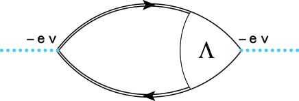
Figure 1: Diagrammatic representation of the Kubo equation for the electrical conductivity. The external field coupling to fermion charge times their velocity is shown as a dotted line. The lines are exact single-particle Green’s functions $G$. $\Lambda$ is the renormalized current vertex.

The interesting and hard part for a calculation of the conductivity is the calculation of the external field (EF) - electron vertex $\Lambda$. We structure our calculation applying the Baym–Kadanoff conserving scheme [55, 61, 62] to the QXY-F model and an extension to collective fluctuations of the Memory matrix formalism used in [56, 57]. The inter-relationship of the Memory matrix method to the more familiar many body techniques in quantum field theory [63, 64], used for example to derive the Landau-Boltzmann transport equations, is given below.

II.1 Self-energies and Vertices

Let $D({\bf q},i\nu_{l})$ be the propagator of the collective modes with which the fermions scatter with a coupling function to them $g({\bf p-p}^{\prime})$. The imaginary parts of the retarded self-energies $\Pi_{R}({\bf q},\nu)$ for the collective modes and $\Sigma_{R}({\bf p},\varepsilon)$ for the fermions are represented diagrammatically by Fig. 2 and are given by,

$${\rm Im}\Pi_{R}(q) = -\pi\sinh\frac{\nu}{2T}\int_{p}\,|g({\bf q})|^{2}A(p)A(p\!-\!q){\rm sech}\frac{\varepsilon}{2T}{\rm sech}\frac{\varepsilon\!-\!\nu}{2T},$$ (4)

$${\rm Im}\Sigma_{R}(p) = \frac{1}{2}\cosh\frac{\varepsilon}{2T}\int_{p^{\prime}}\,|g({\bf p}\!-\!{\bf p}^{\prime})|^{2}{\rm Im}D_{R}(p\!-\!p^{\prime})A(p^{\prime}){\rm cosech}\frac{\varepsilon\!-\!\varepsilon^{\prime}}{2T}{\rm sech}\frac{\varepsilon^{\prime}}{2T},$$ (5)

where $A(p)$ is the single-particle spectral function,

$$A(p)=-\frac{1}{\pi}{\rm Im}G_{R}(p).$$ (6)

Here we have introduced the $(d+1)$-momentum notation $q=({\bf q},\nu)$, $p=({\bf p},\varepsilon)$, and $p^{\prime}=({\bf p},\varepsilon^{\prime})$ along with abbreviations such as $\int_{p}=V^{-1}\sum_{\bf p}\int_{-\infty}^{\infty}d\varepsilon$ for brevity.

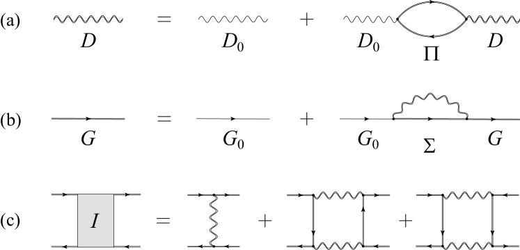
Figure 2: Diagrammatic representation of (a) the renormalized collective mode propagator. In our case, the exact collective mode propagator is already available from quantum Monte-carlo and renormalization group calculations. (b) the renormalized fermion propagator and (c) the irreducible vertex.

The Monte-carlo calculations of the critical fluctuations of the quantum xy model on a lattice with coupling to fermions provides the collective fluctuation propagator $D$ including its self-energy through coupling to fermions and Umklapp scattering due to the square lattice. Therefore, we shall not need $D_{0}$ in Fig. 2(a) explicitly but the fact that $D$ is a functional of the fermion propagator is important to note for calculating the vertex, as shown below. The availability of the renormalized propagator of the fluctuations for the wiggly lines in Fig. 2 so that they need not be re-calculated in the evaluation of the fermion-vertices below is crucial for the developments below.

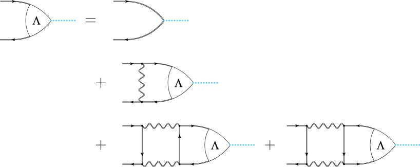
Figure 3: Diagrammatic representation for the integral equation for the external Field vertices in calculation of conductivity. This is a sum of three parts shown successively in the three lines. First is the vertex coupling to the renormalized fermion propagators, second and third are the vertex coupling to the collective modes. The second line gives what may be called ”Maki-Thompson” diagrams and the third corresponds to the ”Aslamazov-Larkin” diagrams

The irreducible vertex $I$, represented in Fig. 2(c) (using which one can calculate the vertex $\Lambda$ as well as the fermion self-energy) is given by the functional derivative $I=\delta\Sigma/\delta G$ [61, 62]. Because the exact Green’s function $D$ is a functional of $G$, the irreducible vertex $I$ includes contributions not only from what might be called the Maki-Tompson (MT) type diagram (the second line in the diagrams shown in Fig. 3) but also from the two Aslamazov-Larkin (AL) type diagrams (the third line in the digram), thorough the functional derivative of $D$ with respect to $G$. We will find that the MT type diagrams do not contribute for the present problem but the AL diagrams are essential for providing the Umklapp factor. Also the first line of Fig. 3 gives no correction from the self-energy of the propagator and is therefore just the bare velocity. This as well as the absence of the MT diagram was noted earlier [65] but the contribution of the AL diagrams was not noted.

We will need the analytic continuation of the EF electron vertex part given by an integral equation represented in Fig. 3. This is accomplished following the classic paper by Èliashberg [66]. By taking $i\omega_{m}\to\omega+i0^{+}$ with $\omega=0$ after the analytic continuation of $\Lambda({\bf p},i\epsilon_{n};i\omega_{m})$ to the region 2 shown by Fig. 4(a) on the complex energy plane of $i\epsilon_{n}=z$, we obtain

$$\Lambda_{2}(p) = {\tilde{v}}_{x}(p)+\frac{1}{2\pi}\cosh\frac{\varepsilon}{2T}\int_{p^{\prime}}\,{\cal I}(p,p^{\prime})\,{\rm sech}\frac{\varepsilon^{\prime}}{2T}G_{R}(p^{\prime})G_{A}(p^{\prime})\Lambda_{2}(p^{\prime}).$$ (7)

$\Lambda_{2}$ alone will enter in subsequent calculations. Its definition follows Èliashberg; The first term on the right comes from the diagrams including $G_{R}G_{R}$ and $G_{A}G_{A}$ and they satisfies the Ward identity or the continuity equation,

$${\tilde{v}}_{x}(p)=v_{{\bf p}x}+\frac{\partial\,{\rm Re}\Sigma_{R}(p)}{\partial p_{x}}.$$ (8)

The second term comes from the particle-hole sections with $G_{R}G_{A}$ and ${\cal I}(p,p^{\prime})$ is given by

$${\cal I}(p,p^{\prime}) = -\frac{1}{2i}\left[I_{22}^{\,{\rm II}}(p,p^{\prime})-I_{22}^{\,{\rm III}}(p,p^{\prime})\right]{\rm cosech}\frac{\varepsilon-\varepsilon^{\prime}}{2T}$$ (9)

$$+\frac{1}{2i}\left[I_{22}^{\,{\rm III}}(p,p^{\prime})-I_{22}^{\,{\rm IV}}(p,p^{\prime})\right]{\rm cosech}\frac{\varepsilon+\varepsilon^{\prime}}{2T},$$

where $I_{22}^{\,{\rm II}}$, $I_{22}^{\,{\rm III}}$, and $I_{22}^{\,{\rm IV}}$ are the analytic continuations of the irreducible vertex $I({\bf p},i\epsilon_{n},{\bf p}^{\prime},i\epsilon_{n^{\prime}};i\omega_{m})$ to the regions shown by Fig. 4(b) with $i\epsilon_{n}=z$ and $i\epsilon_{n^{\prime}}=z^{\prime}$. Note that the conservation of charge leads to a Ward–Takahashi identity that relates the imaginary part of the fermion self-energy to the irreducible vertex as

$$2{\rm Im}\Sigma_{R}(p)\,{\rm sech}\frac{\varepsilon}{2T} = -\int_{p^{\prime}}\,{\cal I}(p,p^{\prime})A(p^{\prime}){\rm sech}\frac{\varepsilon^{\prime}}{2T}.$$ (10)

By use of ${\tilde{v}}_{x}(p)$ and $\Lambda_{2}(p)$, the Kubo formula, Eq. (1), can be written for $\omega=0$ as

$$\sigma(T)=\frac{e^{2}}{\pi}\int_{p}\,\left(-\frac{\partial f(\varepsilon)}{\partial\varepsilon}\right){\tilde{v}}_{x}(p)G_{R}(p)G_{A}(p)\Lambda_{2}(p),$$ (11)

where $-\partial f(\varepsilon)/\partial\varepsilon=(1/4T)\,{\rm sech}^{2}(\varepsilon/2T)$.

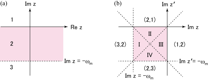
Figure 4: Regions on the complex energy plane for the analytic continuations of (a) $\Lambda({\bf p},z;i\omega_{m})$ with $i\epsilon_{n}=z$ and (b) $I({\bf p},i\epsilon_{n},{\bf p}^{\prime},i\epsilon_{n^{\prime}};i\omega_{m})$ with $i\epsilon_{n}=z$ and $i\epsilon_{n^{\prime}}=z^{\prime}$.

We introduce the electron velocity distribution function $\Phi(p)$, which occurs in Boltzmann equation for transport. We now conveniently re-write the Kubo formula, Eq. (1) in terms of $\Phi(p)$ instead of $\Lambda_{2}(p)$ as promised earlier in Eq. (3),

$$\Phi(p)=-\frac{\Lambda_{2}(p)}{2{\rm Im}\Sigma_{R}(p)}.$$ (12)

Noting that

$$G_{R}(p)G_{A}(p)=\frac{{\rm Im}G_{R}(p)}{{\rm Im}\Sigma_{R}(p)},$$ (13)

we can rewrite Eqs. (7) and (11) so that the electrical conductivity, including its $\omega$ dependence is given by

$$\sigma(\omega,T)=2e^{2}\int_{p}\,\frac{1}{4T}\,{\rm sech}^{2}\frac{\varepsilon}{2T}{\tilde{v}}_{x}(p)A(p)\Phi(p,\omega).$$ (14)

The velocity distribution function $\Phi(p,\omega)$ satisfies

$${\tilde{v}}_{x}(p)\,{\rm sech}\frac{\varepsilon}{2T} = \left[-i\omega a^{-1}(p)+2{\tilde{\Gamma}}(p)\right]\Phi(p)\,{\rm sech}\frac{\varepsilon}{2T}$$ (15)

$$-\int_{p^{\prime}}\,\left[-i\omega\Gamma^{k}(p,p^{\prime})\frac{1}{4T}\,{\rm sech}\frac{\varepsilon}{2T}\,{\rm sech}\frac{\varepsilon^{\prime}}{2T}+{\cal I}(p,p^{\prime})\right]$$

$$\times A(p^{\prime})\Phi(p^{\prime},\omega)\,{\rm sech}\frac{\varepsilon^{\prime}}{2T},$$

where $a(p)^{-1}=1-\partial{\rm Re}\Sigma_{R}(p)/\partial\varepsilon$, ${\tilde{\Gamma}}(p)=-{\rm Im}\Sigma_{R}(p)$, and $\Gamma^{k}(p,p^{\prime})$ is the full four-point vertex in the $k\to 0$ before $\omega\to 0$ limit. Here ${\cal I}(p,p^{\prime})$ is the contributions from the three processes shown in Fig. 2(c) for which Eq. (9) leads to

$${\cal I}(p,p^{\prime}) = -|g({\bf p}\!-\!{\bf p}^{\prime})|^{2}{\rm Im}D_{R}(p\!-\!p^{\prime}){\rm cosech}\frac{\varepsilon\!-\!\varepsilon^{\prime}}{2T}$$ (16)

$$+\pi\int_{p_{1}}\,|g({\bf p}\!-\!{\bf p}_{1})|^{4}D_{R}(p\!-\!p_{1})D_{A}(p\!-\!p_{1})$$

$$\times\left(A(p_{1})A(p_{1}\!-\!p\!+\!p^{\prime}){\rm sech}\frac{\varepsilon_{1}}{2T}{\rm sech}\frac{\varepsilon_{1}\!-\!\varepsilon\!+\!\varepsilon^{\prime}}{2T}\right.$$

$$-\left.A(p_{1})A(p\!+\!p^{\prime}\!-\!p_{1}){\rm sech}\frac{\varepsilon_{1}}{2T}{\rm sech}\frac{\varepsilon\!+\!\varepsilon^{\prime}\!-\!\varepsilon_{1}}{2T}\right).$$

The first and second terms on the right come from the MT and AL type diagrams, respectively. Noting that

$$D_{R}(q)D_{A}(q)=\frac{{\rm Im}D_{R}(q)}{{\rm Im}\Pi_{R}(q)},$$ (17)

we can rewrite Eq. (16) as

$${\cal I}(p,p^{\prime}) = \pi W(p\!-\!p^{\prime})\int_{p_{1}}\,A(p_{1})A(p_{1}\!-\!p\!+\!p^{\prime})\,{\rm sech}\frac{\varepsilon_{1}}{2T}\,{\rm sech}\frac{\varepsilon_{1}\!-\!\varepsilon\!+\!\varepsilon^{\prime}}{2T}$$ (18)

$$+\pi\int_{p_{1}}\,W(p\!-\!p_{1})\left(A(p_{1})A(p_{1}\!-\!p\!+\!p^{\prime})\,{\rm sech}\frac{\varepsilon_{1}}{2T}\,{\rm sech}\frac{\varepsilon_{1}\!-\!\varepsilon\!+\!\varepsilon^{\prime}}{2T}\right.$$

$$-\left.A(p_{1})A(p\!+\!p^{\prime}\!-\!p_{1})\,{\rm sech}\frac{\varepsilon_{1}}{2T}\,{\rm sech}\frac{\varepsilon\!+\!\varepsilon^{\prime}\!-\!\varepsilon_{1}}{2T}\right),$$

where

$$W(q)=\frac{|g({\bf q})|^{4}{\rm Im}D_{R}(q)}{{\rm Im}\Pi_{R}(q)}.$$ (19)

Then Eq. (15) with $\omega=0$ can be written as

$${\tilde{v}}_{x}(p)\,{\rm sech}\frac{\varepsilon}{2T} = \pi\int_{p^{\prime}}\!\int_{p_{1}}\,W(p-p^{\prime})A(p_{1})A(p-p^{\prime}+p_{1})A(p^{\prime})$$ (20)

$$\times\big{[}\Phi(p)-\Phi(p^{\prime})+\Phi(p_{1})-\Phi(p-p^{\prime}+p_{1})\big{]}$$

$$\times\,{\rm sech}\frac{\varepsilon_{1}}{2T}\,{\rm sech}\frac{\varepsilon-\varepsilon^{\prime}+\varepsilon_{1}}{2T}\,{\rm sech}\frac{\varepsilon^{\prime}}{2T}.$$

Assuming Landau’s quasiparticles, we can show that Eqs. (3) and (14) are equivalent, and Eq. (20) corresponds to the Boltzmann equation for the problem of transport for fermions coupled to collective fluctuations in the limit of vanishing external frequency and wave vector. This is accomplished in Appendix B, but here we proceed without such an assumption.

II.2 Memory matrix formalism

Introducing the dimensionless energy variables scaled by temperature and omitting the momentum variables for brevity, we use an abbreviated notation in which $A(t)=A({\bf p},Tt)$, ${\tilde{\Gamma}}(t)={\tilde{\Gamma}}({\bf p},Tt)$, and ${\cal I}(t,t^{\prime})={\cal I}({\bf p},Tt,{\bf p}^{\prime},Tt^{\prime})$. We can then write Eq. (14) and (15) as

$$\sigma(\omega,T) = 2\int_{-\infty}^{\infty}dtX_{1}(t)A(t)\Phi_{1}(t),$$ (21)

$$X_{1}(t) = -i\omega\Phi_{1}(t)-i\int_{-\infty}^{\infty}dt^{\prime}M(t,t^{\prime})A(t^{\prime})\Phi_{1}(t^{\prime}),$$ (22)

where $X_{1}(t)=-e{\tilde{v}}_{x}({\bf p},Tt)(1/2)\,{\rm sech}(t/2)$, $\Phi_{1}(t)=\Phi({\bf p},Tt)(1/2)\,{\rm sech}(t/2)$, and $M(t,t^{\prime})=M^{\prime}(t,t^{\prime})+iM^{\prime\prime}(t,t^{\prime})$ is the memory matrix with

$$M^{\prime}(t,t^{\prime}) = \omega\left(a^{-1}-1\right)A^{-1}(t)\delta(t-t^{\prime})-\omega\Gamma^{k}\frac{1}{4}\,{\rm sech}\frac{t}{2}\,{\rm sech}\frac{t^{\prime}}{2},$$ (23)

$$M^{\prime\prime}(t,t^{\prime}) = 2{\tilde{\Gamma}}(t)A^{-1}(t)\delta(t-t^{\prime})-T{\cal I}(t,t^{\prime}).$$ (24)

In Eqs. (21) and (22), the sum with respect to the momentum is implicit. From Eq. (22), $\Phi_{1}(t)=i\int dt^{\prime}[\omega\delta(t-t^{\prime})+M(t,t^{\prime})A(t^{\prime})]^{-1}X_{1}(t^{\prime})$, so that the electrical conductivity can be written using the memory matrix,

$$\sigma(\omega,T) = 2i\int_{-\infty}^{\infty}dtdt^{\prime}X_{1}(t)[\omega A^{-1}(t)\delta(t-t^{\prime})+M(t,t^{\prime})]^{-1}X_{1}(t^{\prime}).$$ (25)

At low temperatures, the single-particle spectral functions $A(t)=A({\bf p},Tt)$ in Eqs. (23)–(25) can be replaced by $A_{0}=A({\bf p},0)$. All the functions with this replacement are then distinguished by the subscript $0$. For a metal with a Fermi-surface satisfying Luttinger’s theorem, $A({\bf p},0)=\delta({\tilde{\epsilon}}_{\bf p})$, where ${\tilde{\epsilon}}_{\bf p}={\epsilon}_{\bf p}+{\rm Re}\Sigma_{R}({\bf p},0)$ with ${\epsilon}_{\bf p}$ giving the non-interacting energy dispersion relative to the chemical potential. Thus, at the lowest order in temperature, the momentum summation is restricted on the Fermi-surface. Now we define the inner product in this restricted momentum space as $\langle u|v\rangle=(2\pi)^{-d}\int d{\bf p}\,u_{\bf p}v_{\bf p}\delta({\tilde{\epsilon}}_{\bf p})/N(0)$ with $N(0)=(2\pi)^{-d}\int d{\bf p}\,\delta({\tilde{\epsilon}}_{\bf p})$, and ${\hat{M}}|u\rangle=(2\pi)^{-d}\int d{{\bf p}^{\prime}}M_{{\bf p}{\bf p}^{\prime}}u_{{\bf p}^{\prime}}\delta({\tilde{\epsilon}}_{{\bf p}^{\prime}})/N(0)$. (We take the limit of infinite volume so that $V^{-1}\sum_{\bf p}\to(2\pi)^{-d}\int d{\bf p}$.) Then the leading term of Eq. (25) with respect to temperature is given by

$$\sigma(\omega,T) = 2ie^{2}N(0)\int_{-\infty}^{\infty}dtdt^{\prime}\langle{\tilde{v}}_{x}|[\omega\hat{1}\delta(t-t^{\prime})+{\hat{M}}_{0}(t,t^{\prime})]^{-1}|{\tilde{v}}_{x}\rangle\frac{1}{4}\,{\rm sech}\frac{t}{2}\,{\rm sech}\frac{t^{\prime}}{2},$$ (26)

where $|{\tilde{v}}_{x}\rangle$ represents the vector for ${\tilde{v}}_{{\bf p}x}=\partial{\tilde{\epsilon}}_{\bf p}/\partial p_{x}$ in this inner product space.

As pointed out in [56], the imaginary part of the memory matrix has zero eigenvalues when the system described by a Hamiltonian $H$ has conserved quantities. This is because a conservation law $[Q,H]=0$ with $Q=\sum_{{\bf p},\sigma}\theta_{\bf p}c^{\dagger}_{{\bf p},\sigma}c_{{\bf p},\sigma}$ leads to the Generalized Ward-Takahashi identity,

$$2{\rm Im}\Sigma_{R}(p)\theta_{\bf p}\,{\rm sech}\frac{\varepsilon}{2T} = -\int_{p^{\prime}}\,{\cal I}(p,p^{\prime})A(p^{\prime})\theta_{{\bf p}^{\prime}}{\rm sech}\frac{\varepsilon^{\prime}}{2T}.$$ (27)

In a lattice, the total momentum is not strictly a conserved quantity if Umklapp scattering is allowed. At low temperatures, however, all the momentum involved in scattering must be on the Fermi-surface, so Umklapp scattering is ineffective in a system with a small Fermi-surface so that momentum is conserved. In that case, $\theta_{\bf p}=p_{x}$ and we have

$$\int_{-\infty}^{\infty}dt^{\prime}\hat{M}^{\prime\prime}_{0}(t,t^{\prime})|\theta\rangle\,{\rm sech}\frac{t^{\prime}}{2}=0.$$ (28)

Since $p_{x}$ has an overlap with ${\tilde{v}}_{{\bf p}x}$ on the Fermi-surface, the resistivity vanishes and Eq. (26) takes the form of $\sigma(\omega,T)=D^{T}/(-i\pi\omega)$ at low but nonzero temperatures. Note that $D^{T}$ differs from the usual Drude weight $D^{\omega}$ that is defined at zero temperature [56]. From Eq. (23), $D^{T}=4\pi e^{2}\langle{\tilde{v}}_{x}|\theta\rangle^{2}/\chi_{\theta\theta}$ with $\theta_{\bf p}=p_{x}$, where $\langle{\tilde{v}}_{x}|\theta\rangle=n/2$ with the electron number density $n$ and $\chi_{\theta\theta}$ is the static limit of the momentum autocorrelation function, as pointed out in [59].

As will be shown in the next sub-section, when the critical fluctuations scale as a function of $\omega/T$, in other words, when the imaginary part of the propagator of the collective modes is as ${\rm Im}D_{R}({\bf q},\omega)={\cal F}_{\bf q}(\omega/T)$, the imaginary part of the memory matrix is proportional to temperature, i.e., $\hat{M}^{\prime\prime}_{0}(t,t^{\prime})\propto T$. If there is a conserved quantity so that $\hat{M}_{0}^{\prime\prime}(t,t^{\prime})$ has a zero eigenvalue as described by Eq. (28), $\sigma(\omega,T)\propto-i/\omega$ with a vanishing linear in $T$ resistivity. This is true for small Fermi-surfaces where Umklapp is ineffective. However, as will be demonstrated in Sec. II-E, for large Fermi-surfaces where Umklapp scattering occurs, there is no such conserved quantity and a nonzero linear in $T$ resistivity results. Since the real part $\hat{M}^{\prime}_{0}(t,t^{\prime})$ of the memory matrix is proportional to $\omega$, Eq. (26) shows that the electrical conductivity then scales as a function of $\omega/T$ and may be written as $\sigma(\omega,T)=T^{-1}{\cal G}(\omega/T)$ with ${\cal G}(0)$ finite. Therefore, when the Fermi-surface is large and the critical fluctuations obey a $\omega/T$ scaling, the quantum-critical conductivity also obeys a $\omega/T$ scaling.

II.3 Low-temperature electrical and thermal conductivities

The dc-electrical conductivity $\sigma$ and the thermal conductivity $\kappa$ can be written using the transport coefficients $L_{ij}$ as

$$\sigma = L_{11},$$ (29)

$$\kappa = \frac{1}{T}\left(L_{22}-\frac{L_{12}L_{21}}{L_{11}}\right).$$ (30)

Here $L_{11}$ is given by Eq. (21) for $\omega=0$, which is derived from the Kubo formula, while $L_{12}$ ($=$ $L_{21}$) and $L_{22}$ are usually derived by analogy from the Boltzmann transport theory [67], but for strongly correlated electron systems with short-range Coulomb interactions they are justified on the basis of the Kubo-Luttinger formalism [68, 69, 70]. Introducing $X_{2}(t)=T{\tilde{v}}_{x}({\bf p},Tt)(t/2)\,{\rm sech}(t/2)$ in addition to $X_{1}(t)$, these transport coefficients can be written together as

$$L_{ij} = 2\int_{-\infty}^{\infty}dtX_{i}(t)A(t)\Phi_{j}(t),$$ (31)

where $\Phi_{i}(t)$ ($i=1,2$) is the solution of the integral equation,

$$X_{i}(t) = \int_{-\infty}^{\infty}dt^{\prime}M^{\prime\prime}(t,t^{\prime})A(t^{\prime})\Phi_{i}(t^{\prime})$$ (32)

$$= 2{\tilde{\Gamma}}(t)\Phi_{i}(t)-T\int_{-\infty}^{\infty}dt^{\prime}{\cal I}(t,t^{\prime})A(t^{\prime})\Phi_{i}(t^{\prime}).$$

This equation for $i=1$ corresponds to Eq. (22) with $\omega=0$.

Now we assume that the low-temperature expansion of the spectral function $A(t)$ can be written as $A(t)=A_{0}+A_{1}(t)+\cdots$ with $A_{0}=\delta({\tilde{\epsilon}}_{\bf p})$. Then, applying this expansion to the spectral functions in Eqs. (5) and (16), the self-energy and vertex parts can be expanded as ${\tilde{\Gamma}}(t)={\tilde{\Gamma}}_{0}(t)+{\tilde{\Gamma}}_{1}(t)+\cdots$ and ${\cal I}(t,t^{\prime})={\cal I}_{0}(t,t^{\prime})+{\cal I}_{1}(t,t^{\prime})+\cdots$, respectively. Let us write $Y_{i}(t)$ for the leading term in the low-temperature expansion of $\Phi_{i}(t)$, which satisfies

$$X_{i}(t) = \int_{-\infty}^{\infty}dt^{\prime}M_{0}^{\prime\prime}(t,t^{\prime})A_{0}Y_{i}(t^{\prime})$$ (33)

$$= 2{\tilde{\Gamma}}_{0}(t)Y_{i}(t)-T\int_{-\infty}^{\infty}dt^{\prime}{\cal I}_{0}(t,t^{\prime})A_{0}Y_{i}(t^{\prime}).$$

Then the leading term of the diagonal transport coefficient is simply given by

$$L_{ii}=2\int_{-\infty}^{\infty}dtX_{i}(t)A_{0}Y_{i}(t).$$ (34)

However, $X_{1}(t)$ and $Y_{2}(t)$ are even and odd functions of $t$, respectively, so $\int_{-\infty}^{\infty}dtX_{1}(t)A_{0}Y_{2}(t)$ $=$ $0$. Hence the off-diagonal transport coefficient requires higher-order expansions, and its leading term takes a rather complicated form,

$$L_{12} = 4\int_{-\infty}^{\infty}dtY_{1}(t){\tilde{\Gamma}}_{0}(t)A_{1}(t)Y_{2}(t)$$ (35)

$$-4\int_{-\infty}^{\infty}dtY_{1}(t){\tilde{\Gamma}}_{1}(t)A_{0}Y_{2}(t)$$

$$+2T\int_{-\infty}^{\infty}dtdt^{\prime}Y_{1}(t)A_{0}{\cal I}_{1}(t,t^{\prime})A_{0}Y_{2}(t^{\prime}).$$

Since $L_{12}$ ($=$ $L_{21}$) arises from the higher-order terms in the low-temperature expansion, $L_{12}L_{21}\ll L_{11}L_{22}$, and thus the thermal conductivity is given by $\kappa=L_{22}/T$ at low temperatures. Then, from Eqs. (33) and (34), $\kappa$ as well as $\sigma$ can be obtained using the imaginary part $M_{0}^{\prime\prime}(t,t^{\prime})$ of the memory matrix whose momenta are limited on the Fermi-surface due to the presence of $A_{0}=\delta({\tilde{\epsilon}}_{\bf p})$.

For specific calculations of $\sigma$ and $\kappa$, it is useful to introduce the Fermi-surface harmonics $\psi_{L}({\bf p})$ which are orthonormalized as $\langle\psi_{L}|\psi_{L^{\prime}}\rangle=(2\pi)^{-d}\int d{\bf p}\psi_{L}({\bf p})\psi_{L^{\prime}}({\bf p})\delta({\tilde{\epsilon}}_{\bf p})/N(0)=\delta_{L,L^{\prime}}$ and complete $\sum_{L}|\psi_{L}\rangle\langle\psi_{L}|=\hat{1}$. Since the bare vertex is an odd function of momentum, only the harmonics satisfying $\psi_{L}(-{\bf p})=-\psi_{L}({\bf p})$ can form a basis and $\psi_{L}({\bf p})$ with $L=1$ is chosen to be proportional to ${\tilde{v}}_{{\bf p}x}$, i.e., $\psi_{1}({\bf p})={\tilde{v}}_{{\bf p}x}/\langle{\tilde{v}}_{x}^{2}\rangle^{1/2}$ where $\langle{\tilde{v}}_{x}^{2}\rangle=\langle{\tilde{v}}_{x}|{\tilde{v}}_{x}\rangle$ is the average of ${\tilde{v}}_{x}^{2}$ on the Fermi-surface. Using this basis of the Fermi-surface harmonics and denoting the elements of the memory matrix as $[\hat{M}(t,t^{\prime})]_{LL^{\prime}}\equiv\langle\psi_{L}|\hat{M}(t,t^{\prime})|\psi_{L^{\prime}}\rangle$, Eq. (26) with $\omega=0$ can be written as

$$\sigma = 2e^{2}N(0)\langle{\tilde{v}}_{x}^{2}\rangle\int_{-\infty}^{\infty}dtdt^{\prime}\frac{[\hat{M}_{0}^{\prime\prime}(t,t^{\prime})^{-1}]_{11}}{4\cosh(t/2)\cosh(t^{\prime}/2)}.$$ (36)

From the consideration in the previous paragraph, the thermal conductivity at low temperatures can also be written in a similar form,

$$\kappa =2TN(0)\langle{\tilde{v}}_{x}^{2}\rangle\int_{-\infty}^{\infty}dtdt^{\prime}\frac{[\hat{M}_{0}^{\prime\prime}(t,t^{\prime})^{-1}]_{11}tt^{\prime}}{4\cosh(t/2)\cosh(t^{\prime}/2)}.$$ (37)

From Eq. (24) with Eqs. (5), (16), and (18), the imaginary part of the memory matrix can be obtained as

$$\hat{M}^{\prime\prime}_{0}(t,t^{\prime})=\hat{M}^{\prime\prime}_{\rm SE}(t,t^{\prime})+\hat{M}^{\prime\prime}_{\rm MT}(t,t^{\prime})+\hat{M}^{\prime\prime}_{\rm AL}(t,t^{\prime}),$$ (38)

where the first, second, and third terms are the contributions from the self-energy, MT-vertex, and AL-vertex corrections, respectively, (from which the subscripts $0$’s are omitted for brevity) and their matrix elements are given by

$$[\hat{M}_{\rm SE}^{\prime\prime}(t,t^{\prime})]_{LL^{\prime}}= -\frac{T}{N(0)}\int\frac{d{\bf p}\,d{\bf p}^{\prime}}{(2\pi)^{2d}}\psi_{L}({\bf p})\psi_{L^{\prime}}({\bf p})\delta({\tilde{\epsilon}}_{\bf p})\delta({\tilde{\epsilon}}_{{\bf p}^{\prime}})$$

$$\times\int_{-\infty}^{\infty}dx|g({\bf p}\!-\!{\bf p}^{\prime})|^{2}{\rm Im}D_{R}({\bf p}-{\bf p}^{\prime},Tx)$$

$$\times\delta(t-t^{\prime})\cosh\frac{t}{2}\,{\rm sech}\frac{t-x}{2}\,{\rm cosech}\frac{x}{2},$$ (39)

$$[\hat{M}_{\rm MT}^{\prime\prime}(t,t^{\prime})]_{LL^{\prime}}= \frac{T}{N(0)}\int\frac{d{\bf p}\,d{\bf p}^{\prime}}{(2\pi)^{2d}}\psi_{L}({\bf p})\delta({\tilde{\epsilon}}_{\bf p})\delta({\tilde{\epsilon}}_{{\bf p}^{\prime}})\psi_{L^{\prime}}({\bf p}^{\prime})$$

$$\times|g({\bf p}\!-\!{\bf p}^{\prime})|^{2}{\rm Im}D_{R}({\bf p}-{\bf p}^{\prime},Tt-Tt^{\prime})$$

$$\times\,{\rm cosech}\frac{t-t^{\prime}}{2},$$ (40)

$$[\hat{M}_{\rm AL}^{\prime\prime}(t,t^{\prime})]_{LL^{\prime}}= \frac{T}{2N(0)}\int\frac{d{\bf p}\,d{\bf p}^{\prime}}{(2\pi)^{2d}}\psi_{L}({\bf p})\delta({\tilde{\epsilon}}_{\bf p})\delta({\tilde{\epsilon}}_{{\bf p}^{\prime}})$$

$$\times\int\frac{d{\bf k}d{\bf k}^{\prime}}{(2\pi)^{d}}\Delta^{d}({\bf p}-{\bf p}^{\prime}+{\bf k}-{\bf k}^{\prime})\delta({\tilde{\epsilon}}_{\bf k})\delta({\tilde{\epsilon}}_{{\bf k}^{\prime}})\psi_{L^{\prime}}({\bf k}^{\prime})$$

$$\times\left[\int\frac{d{\bf k}_{1}d{\bf k}_{1}^{\prime}}{(2\pi)^{d}}\Delta^{d}({\bf p}-{\bf p}^{\prime}+{\bf k}_{1}-{\bf k}_{1}^{\prime})\delta({\tilde{\epsilon}}_{{\bf k}_{1}})\delta({\tilde{\epsilon}}_{{\bf k}_{1}^{\prime}})\right]^{-1}$$

$$\times\int_{-\infty}^{\infty}dx|g({\bf p}\!-\!{\bf p}^{\prime})|^{2}{\rm Im}D_{R}({\bf p}-{\bf p}^{\prime},Tx)$$

$$\times\frac{1}{x}\,{\rm sech}\frac{t-x}{2}\left({\rm sech}\frac{t^{\prime}+x}{2}+\,{\rm sech}\frac{t^{\prime}-x}{2}\right).$$ (41)

Here $\Delta^{d}({\bf p}-{\bf p}^{\prime}-{\bf q})\equiv\sum_{\bf G}\delta^{d}({\bf p}-{\bf p}^{\prime}-{\bf q}-{\bf G})$ is a $d$-dimensional delta function extended to the lattice with ${\bf G}$ being the reciprocal lattice vectors including a zero vector, and then normal and Umklapp scatterings are described by ${\bf G}={\bf 0}$ and ${\bf G}\neq{\bf 0}$, respectively. Note that the AL contribution is generally particle-hole asymmetric, which is essential for the Seebeck coefficient discussed in Sec. II-F, but its leading term given by Eq. (41) in the low-temperature expansion has particle-hole symmetry expressed as $\hat{M}^{\prime\prime}_{\rm AL}(t,t^{\prime})=\hat{M}^{\prime\prime}_{\rm AL}(t,-t^{\prime})=\hat{M}^{\prime\prime}_{\rm AL}(-t,t^{\prime})$, while the bare vertex for $\kappa$ is an odd function of the energy variable. Thus the AL vertex corrections do not contribute to the leading term in $\kappa$, but they do for $\sigma$.

From these equations, we immediately find that when the imaginary part of the propagator of the collective modes is written as ${\rm Im}D_{R}({\bf q},\omega)={\cal F}_{\bf q}(\omega/T)$, the imaginary part of the memory matrix is proportional to temperature, i.e., $\hat{M}^{\prime\prime}_{0}(t,t^{\prime})\propto T$. Note that the eigenfunction with the zero eigenvalue described by Eq. (28) is an even function of the energy variable $t^{\prime}$, which has an effect only on $\sigma$. On the other hand, the eigenvalues of $\hat{M}^{\prime\prime}_{0}(t,t^{\prime})$ for eigenfunctions that are odd functions of the energy variable are nonzero positive in general. This is related to the symmetry that the AL vertex corrections are absent for $\kappa$. As a result, $\kappa$ is finite even without Umklapp scattering and is a temperature-independent constant from Eq. (37) when $\hat{M}^{\prime\prime}_{0}(t,t^{\prime})\propto T$.

II.4 Marginal Fermi-liquid or Planckian dissipation for criticality of the quantum xy-model coupled to fermions

We use the critical fluctuations and their coupling to fermions summarized in Appendix A, assuming that they are valid for fluctuations of any vector field obeying $U(1)$ symmetry in the quantum-critical region and coupled to fermions as in the model solved in [25, 30, 31, 29]. The self-energy of the fermions is then effectively momentum independent for all calculations so that with the coupling function specified in Appendix A,

$$|g({\bf q})|^{2}{\rm Im}D_{R}({\bf q},\nu)=-\bar{g}^{2}\tanh\left(\frac{\nu}{2T}\right).$$ (42)

From Eq. (5), the full energy and temperature dependences of the imaginary part of the self-energy is given by

$${\rm Im}\Sigma_{R}({\bf p},\varepsilon) =-\bar{g}^{2}N(\varepsilon)\,\varepsilon\coth\frac{\varepsilon}{2T},$$ (43)

where $N(\varepsilon)=(2\pi)^{-d}\int d{\bf p}A({\bf p},\varepsilon)$ is the density of states of fermions per spin. We apply the memory matrix formalism described in the previous section to the case of Eq. (42).

First of all, the momentum independence of Eq. (42) leads to the fact that $\hat{M}^{\prime\prime}_{\rm SE}(t,x)$ is proportional to the unit matrix $\hat{1}$ whose matrix element is $\delta_{L,L^{\prime}}$ and that $\hat{M}^{\prime\prime}_{\rm MT}(t,x)$ vanishes. Then $\hat{M}^{\prime\prime}_{0}(t,x)=\hat{M}^{\prime\prime}_{\rm SE}(t,x)+\hat{M}^{\prime\prime}_{\rm AL}(t,x)$, and Eq. (39) with Eq. (42) leads to

$$\hat{M}^{\prime\prime}_{\rm SE}(t,x) =2\bar{g}^{2}N(0)Tf(t)\delta(t-x)\hat{1},$$ (44)

where

$$f(t) =t\coth(t/2).$$ (45)

The AL vertex corrections can be obtained by substituting Eq. (42) into Eq. (41), as follows:

$$\hat{M}^{\prime\prime}_{\rm AL}(t,x) =-\bar{g}^{2}N(0)T[F(t,x)+F(t,-x)]\hat{B},$$ (46)

where

$$F(t,x) = \frac{1}{4}\int_{-\infty}^{\infty}\frac{dy}{f(y)}\,{\rm sech}\frac{t-y}{2}\,{\rm sech}\frac{y-x}{2},$$ (47)

and the matrix elements of $\hat{B}$ are given by

$$B_{LL^{\prime}} = \frac{2}{N(0)^{2}}\int\frac{d{\bf p}d{\bf p}^{\prime}}{(2\pi)^{2d}}\psi_{L}({\bf p})\delta({\tilde{\epsilon}}_{\bf p})\delta({\tilde{\epsilon}}_{{\bf p}^{\prime}})$$ (48)

$$\times\int\frac{d{\bf k}d{\bf k}^{\prime}}{(2\pi)^{d}}\Delta^{d}({\bf p}-{\bf p}^{\prime}+{\bf k}-{\bf k}^{\prime})\delta({\tilde{\epsilon}}_{\bf k})\delta({\tilde{\epsilon}}_{{\bf k}^{\prime}})\psi_{L^{\prime}}({\bf k}^{\prime})$$

$$\times\left[\int\frac{d{\bf k}_{1}d{\bf k}_{1}^{\prime}}{(2\pi)^{d}}\Delta^{d}({\bf p}-{\bf p}^{\prime}+{\bf k}_{1}-{\bf k}_{1}^{\prime})\delta({\tilde{\epsilon}}_{{\bf k}_{1}})\delta({\tilde{\epsilon}}_{{\bf k}_{1}^{\prime}})\right]^{-1}.$$

Then the effect of the vertex corrections is described by the matrix $\hat{B}$. Gauge invariance relates the vertex corrections to the self-energy as Eq. (10). This relation corresponds to the identity

$$\int_{-\infty}^{\infty}\frac{F(t,x)}{\cosh(x/2)}dx=\frac{f(t)}{\cosh(t/2)}.$$ (49)

Now, following the exact solution of the Boltzmann equation by Jensen, Smith, and Wilkins [71], we consider the eigenvalue equation

$$f(t)\varphi_{n,\pm}(t)=\lambda_{n,\pm}\int_{-\infty}^{\infty}dxF(t,x)\varphi_{n,\pm}(x),$$ (50)

where $\varphi_{n,+}(t)$ and $\varphi_{n,-}(t)$ are even and odd functions of $t$, respectively, $\varphi_{n,\pm}(t)=\pm\varphi_{n,\pm}(\pm t)$, and they are normalized according to

$$\int_{-\infty}^{\infty}dtf(t)\varphi_{n,s}(t)\varphi_{n^{\prime},s^{\prime}}(t)=\delta_{n,n^{\prime}}\delta_{s,s^{\prime}}.$$ (51)

These eigenfunctions and eigenvalues are given by

$$\varphi_{n,+}(t) = \frac{1}{\pi}{\cal P}_{2n-2}(t/\pi)\,{\rm sech}\frac{t}{2},\quad\lambda_{n,+}=(2n-1)^{2},$$ (52)

$$\varphi_{n,-}(t) = \frac{1}{\pi}{\cal P}_{2n-1}(t/\pi)\,{\rm sech}\frac{t}{2},\quad\lambda_{n,-}=(2n)^{2},$$ (53)

where ${\cal P}_{n}(x)$ are orthogonal polynomials in the interval $(-\infty,\infty)$ with a weight function $2x\,{\rm cosech}(\pi x)$, for example, ${\cal P}_{0}(x)=1$, ${\cal P}_{1}(x)=\sqrt{2}x$, and ${\cal P}_{2}(x)=1-2x^{2}$. Note that from Eq. (47) they also satisfy the following auxiliary eigenequation:

$$f(t)\varphi_{n,\pm}(t)=\frac{\sqrt{\lambda_{n,\pm}}}{2}\int_{-\infty}^{\infty}dx\,{\rm sech}\frac{t-x}{2}\varphi_{n,\pm}(x).$$ (54)

All the eigenvalues are grater than or equal to $1$ and the eigenequation for $\varphi_{1,+}(t)=(1/\pi)\,{\rm sech}(t/2)$ with the smallest eigenvalue $\lambda_{1,+}=1$ corresponds to the gauge invariance, Eq. (49).

Using the eigenvalue $\lambda_{n,\pm}\geq 1$ and the eigenfunctions $\varphi_{n,\pm}(t)$, we can write Eqs. (44) and (46) as

$$\hat{M}^{\prime\prime}_{\rm SE}(t,x) =2\bar{g}^{2}N(0)Tf(t)f(x)\sum_{n=1}^{\infty}\sum_{s=\pm}\varphi_{n,s}(t)\varphi_{n,s}(x)\,\hat{1},$$ (55)

$$\hat{M}^{\prime\prime}_{\rm AL}(t,x) =-2\bar{g}^{2}N(0)Tf(t)f(x)\sum_{n=1}^{\infty}\frac{\varphi_{n,+}(t)\varphi_{n,+}(x)}{\lambda_{n,+}}\,\hat{B}.$$ (56)

Therefore we obtain the imaginary part of the memory matrix, $\hat{M}_{0}^{\prime\prime}(t,x)=\hat{M}^{\prime\prime}_{\rm SE}(t,x)+\hat{M}^{\prime\prime}_{\rm AT}(t,x)$, for the MFL

$$\hat{M}_{0}^{\prime\prime}(t,x) = 2\bar{g}^{2}N(0)Tf(t)f(x)\sum_{n=1}^{\infty}\left(\frac{\varphi_{n,+}(t)\varphi_{n,+}(x)}{\lambda_{n,+}}\,(\lambda_{n,+}\hat{1}-\hat{B})+\varphi_{n,-}(t)\varphi_{n,-}(x)\,\hat{1}\right).$$

The inverse matrix can be easily obtained as

$$\hat{M}_{0}^{\prime\prime}(t,x)^{-1} = \frac{1}{2\bar{g}^{2}N(0)T}\sum_{n=1}^{\infty}\left(\varphi_{n,+}(t)\varphi_{n,+}(x)\lambda_{n,+}\,(\lambda_{n,+}\hat{1}-\hat{B})^{-1}+\varphi_{n,-}(t)\varphi_{n,-}(x)\,\hat{1}\right).$$

Since $\hat{M}^{\prime\prime}(t,x)^{-1}\propto 1/T$, we see that the critical fluctuations of the QXY-F model give rise to the Planckian dissipation where the transport relaxation time is proportional to $\hbar/k_{\rm B}T$ (we have re-inserted the Planck constant $\hbar$ and the Boltzmann constant $k_{\rm B}$).

Substituting Eq. (LABEL:inverse_memory) into Eqs. (36) and (37), we obtain.

$$\sigma = \frac{e^{2}\langle{\tilde{v}}_{x}^{2}\rangle}{\bar{g}^{2}T}\sum_{n=1}^{\infty}\left(\int_{-\infty}^{\infty}\frac{\varphi_{n,+}(t)}{2\cosh(t/2)}dt\right)^{2}\left[\frac{\lambda_{n,+}}{\lambda_{n,+}\hat{1}-\hat{B}}\right]_{11},$$ (59)

$$\kappa = \frac{\langle{\tilde{v}}_{x}^{2}\rangle}{\bar{g}^{2}}\sum_{n=1}^{\infty}\left(\int_{-\infty}^{\infty}\frac{t\varphi_{n,-}(t)}{2\cosh(t/2)}dt\right)^{2}.$$ (60)

Note that the effect of the vertex corrections $\hat{B}$ vanishes for the thermal conductivity $\kappa$ due to the symmetry reasons mentioned in the previous sub-section, while the electrical conductivity has the vertex corrections to the self-energy contribution,

$$\sigma_{\rm SE}=\frac{e^{2}\langle{\tilde{v}}_{x}^{2}\rangle}{\bar{g}^{2}T}\sum_{n=1}^{\infty}\left(\int_{-\infty}^{\infty}\frac{\varphi_{n,+}(t)}{2\cosh(t/2)}dt\right)^{2}.$$ (61)

Using the completeness

$$f(t)\sum_{n=1}^{\infty}\sum_{s=\pm}\varphi_{n,s}(t)\varphi_{n,s}(x)=\delta(t-x),$$ (62)

$\sigma_{\rm SE}$ and the thermal conductivity can be calculated as

$$\sigma_{\rm SE} = \frac{e^{2}\langle{\tilde{v}}_{x}^{2}\rangle}{\bar{g}^{2}T}\int_{-\infty}^{\infty}\frac{\tanh(t/2)}{4t\cosh^{2}(t/2)f(t)}dt=\frac{7\zeta(3)}{2\pi^{2}}\frac{e^{2}\langle{\tilde{v}}_{x}^{2}\rangle}{\bar{g}^{2}T},$$ (63)

$$\kappa = \frac{\langle{\tilde{v}}_{x}^{2}\rangle}{\bar{g}^{2}}\int_{-\infty}^{\infty}\frac{t\tanh(t/2)}{4\cosh^{2}(t/2)}dt=\frac{\langle{\tilde{v}}_{x}^{2}\rangle}{\bar{g}^{2}}.$$ (64)

Due to the Planckian dissipation, the thermal conductivity is a constant independent of temperature. The Lorentz number $L$ can then be described by

$$L\equiv\frac{\kappa}{\sigma T}=\frac{\kappa}{\sigma_{\rm SE}T}\frac{\rho}{\rho_{\rm SE}}=\frac{6}{7\zeta(3)}\frac{\rho}{\rho_{\rm SE}}L_{0},$$ (65)

where $\rho=1/\sigma$, $\rho_{\rm SE}=1/\sigma_{\rm SE}$, and $L_{0}=(\pi^{2}/3)(k_{\rm B}/e)^{2}$ is the Lorentz number of normal metals. Since $\frac{6}{7\zeta(3)}=0.713$, the value of $L/L_{0}$ is about 70% of the value of $\rho/\rho_{\rm SE}$.

By using Eq. (61), we can write Eq. (59) as

$$\frac{\sigma}{\sigma_{\rm SE}}=1+\frac{2\pi^{2}}{7\zeta(3)}\sum_{n=1}^{\infty}\left(\int_{-\infty}^{\infty}\frac{\varphi_{n,+}(t)}{2\cosh(t/2)}dt\right)^{2}\left[\frac{\lambda_{n,+}}{(\lambda_{n,+}\!-1)\hat{1}+\hat{C}}-\hat{1}\right]_{11},$$ (66)

where

$$\hat{C}\equiv\hat{1}-\hat{B}.$$ (67)

If we keep only the $n=1$ term in the sum over $n$ in Eq. (66), we obtain the inequality

$$\frac{\sigma}{\sigma_{\rm SE}}>1-\frac{8}{7\zeta(3)}+\frac{8}{7\zeta(3)}[\hat{C}^{-1}]_{11}.$$ (68)

By replacing all eigenvalues $\lambda_{n,+}$ with the minimum eigenvalue $\lambda_{1,+}=1$, on the other hand, we obtain the inequality

$$\frac{\sigma}{\sigma_{\rm SE}}<[\hat{C}^{-1}]_{11}.$$ (69)

Therefore the lower and upper bounds of $\rho/\rho_{\rm SE}$ are given by

$$\left(\frac{\rho}{\rho_{\rm SE}}\right)_{\textrm{L.B.}} = \frac{1}{[\hat{C}^{-1}]_{11}},$$ (70)

$$\left(\frac{\rho}{\rho_{\rm SE}}\right)_{\textrm{U.B.}} = \frac{7\zeta(3)/8}{[\hat{C}^{-1}]_{11}+7\zeta(3)/8-1}.$$ (71)

Since $7\zeta(3)/8=1.0518$, however, these bounds are almost equal, so that we can take the lower bound for evaluating the electrical resistivity. The results for its explicit evaluation for the case of a circular Fermi-surface in a square lattice are given in the next sub-section.

As described in Sec. II-B, if there is a conserved quantity that is odd in time-reversal and in inversion, the imaginary part of the memory matrix has a zero eigenvalue as Eq. (28). By substituting Eq. (LABEL:memory_LCO) for Eq. (28) while noting that $\varphi_{1,+}(t)\propto{\rm sech}(t/2)$, this corresponds to the matrix ${\hat{C}}$ having a zero eigenvalue,

$${\hat{C}}|\theta\rangle=0.$$ (72)

Thus, ${\hat{C}}$ is a matrix describing conservation laws. For the lower bound of $\rho/\rho_{\rm SE}$, we can easily see the relationship between the conservation laws and particle-hole symmetry, since the replacement of all $\lambda_{n,+}$ by 1 in Eq. (LABEL:memory_LCO) leads to

$$\hat{M}_{0}^{\prime\prime}(t,x) \approx 2\bar{g}^{2}N(0)Tf(t)\left\{\left[\delta(t-x)+\delta(t+x)\right]{\hat{C}}+\left[\delta(t-x)-\delta(t+x)\right]{\hat{1}}\right\}.$$ (73)

On the other hand, the upper bound, Eq. (71), shows that $\rho/\rho_{\rm SE}$ vanishes in correspondence with the zero eigenvalues of ${\hat{C}}$.

For a small Fermi-surface where Umklapp scattering is ineffective, the vertex corrections $\hat{B}$ can therefore never be ignored for $\sigma$ because $[\hat{C}^{-1}]_{11}$ diverges due to the momentum conservation. Then the coefficient of the $T$ linear term in the resistivity vanishes. So Umklapp scattering is essential for the linear in $T$ resistivity. However, for the case of the critical fluctuations of the QXY-F model, it provides no temperature dependent factors. This is crucial to be in accord with experiments on single-particle self-energy and the specific heat.

To understand physically that Umklapp scattering is unnecessary for finite thermal conductivity, consider the single-particle decay of thermally excited fermions in the following process: A particle with a momentum ${\bf p}_{1}$ greater than the Fermi momentum $k_{F}$ interacts with a particle inside the Fermi sphere with a momentum ${\bf p}_{2},(|p_{2}|<k_{F})$ and decays into two particles with momenta ${\bf p}_{3}$ and ${\bf p}_{4}$ which are both outside the Fermi sphere. Since momentum is conserved in this process (${\bf p}_{1}+{\bf p}_{2}-{\bf p}_{3}-{\bf p}_{4}=0$), the charge current of the whole system does not decay due to the feedback effect of momentum coming back from other particles. Energy is also conserved in this process: If ${\epsilon}$ is the energy measured from the chemical potential, ${\epsilon}_{1}+{\epsilon}_{2}-{\epsilon}_{3}-{\epsilon}_{4}=0$. However, since ${\epsilon}_{1},{\epsilon}_{3}$, and ${\epsilon}_{4}$ are positive while ${\epsilon}_{2}$ is negative, the product of ${\epsilon}$ and momentum is not conserved. For this reason, the energy current decays even without Umklapp scattering for the fermions, and the thermal conductivity is finite due to normal scattering.

These results can be put in context of the arguments due to Peierls, quoted for example in [67]. Peierls has argued that Umklapp scattering is essential for finite thermal conductivity from phonons in the pure limit, but not for finite electronic thermal conductivity when that is defined, as is customary and done here, making sure that the electronic conductivity induced by thermal gradient is absent. We have substantiated this argument. One should note however that the fermion self-energy $\Sigma$ on a lattice includes the effect of Umklapp scattering so that while one can say that the vertex renormalization is absent for the electronic thermal conductivity, it does not necessarily imply that the Umklapp scattering is absent.

It should be noted that there is no $\log(T)$ correction due to mass renormalization for the electrical conductivity. There is also no $\log(T)$ enhancement of the thermal conductivity which appears in the critical specific heat due to the MFL single-particle quasi-particle renormalization.

Recently, the breakdown of the Wiedemann-Franz law in strongly correlated electron systems and Weyl semimetals has been studied based on the Boltzmann equation [72, 73]. We note that the disappearance of the quasi-particle renormalization in the thermal conductivity is generally true for other problems such as the heavy-Fermi-liquiids, in which the self-energy is nearly momentum independent.

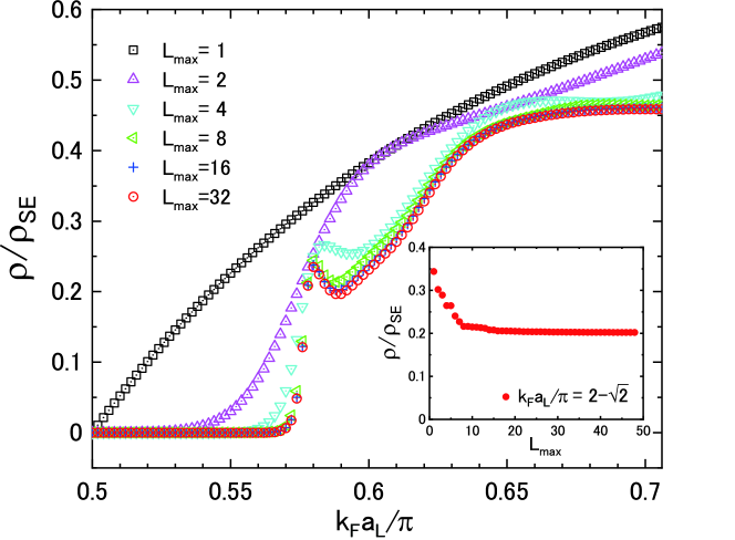
Figure 5: Reduction factor of the electrical resistivity due to the vertex corrections, i.e. the Umklapp factor, for a circular Fermi-surface of radius $k_{F}$ in a square lattice of unit-cell ${a_{L}}$, calculated as a function of $k_{F}{a_{L}}/\pi$ ($1/2<k_{F}{a_{L}}/\pi<1/\sqrt{2})$ for different number of $L_{max}$. The inset shows the $L_{max}$ dependence of the Umklapp factor for $k_{F}{a_{L}}/\pi=2-\sqrt{2}$.

II.5 Results for Umklapp factor on a square lattice with a circular Fermi-surface

The reduction factor $\rho/\rho_{\rm SE}$ of the electrical resistivity due to the vertex corrections is called the Umklapp factor, where $\rho$ is the actual resistivity and $\rho_{\rm SE}$ is the resistivity calculated with self-energy alone, i.e. by putting $\hat{B}=\hat{0}$. As shown in the previous sub-section, the Umklapp factor is given by the inverse of the 11 components of the inverse matrix of $\hat{C}$. For a circular Fermi-surface described by ${\tilde{\epsilon}}_{{\bf p}}\!=\!(p^{2}-k_{F}^{2})/2{\tilde{m}}=0$, from Eqs. (63) and (64), $\rho_{\rm SE}=\frac{2\pi^{2}}{7\zeta(3)}\frac{(\bar{g}{\tilde{m}})^{2}}{\pi ne^{2}}T$ and the $T$ independent thermal conductivity is given by $\kappa=\pi n/(\bar{g}{\tilde{m}})^{2}$ with the electron number density $n$ and the electron unrenormalized mass ${\tilde{m}}$. The evaluation of $\hat{C}=\hat{1}-\hat{B}$ is, however, quite non-trivial even for a circular Fermi-surface and given in Appendix C. The infinite-dimensional matrix $\hat{C}$ can be approximated by a square matrix of $L_{max}\times L_{max}$ and the limit of $L_{max}\to\infty$ gives the correct value. We present the results for numerical evaluation for the Umklapp factor $\rho/\rho_{\rm SE}$ in Fig. 5 for various $L_{max}$ ($=1,2,4,8,16,32$) and for a circular Fermi-surface of radius $k_{F}$ in a square lattice of unit-cell ${a_{L}}$.

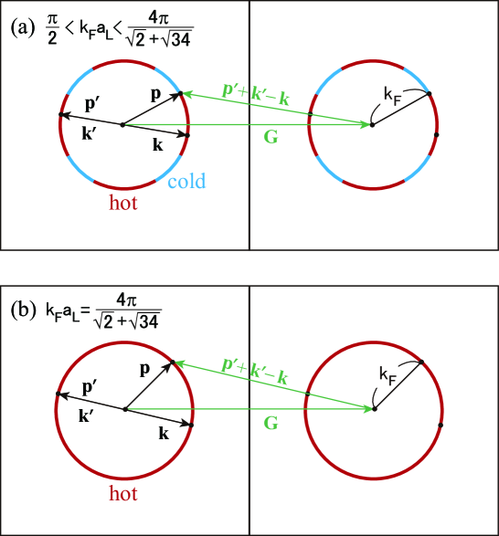
Figure 6: Kinematics of Umklapp scattering for ${\bf p}-{\bf p}^{\prime}+{\bf k}-{\bf k}^{\prime}={\bf G}$ with ${\bf p}^{\prime}={\bf k}^{\prime}=-{\bf k}$ and ${\bf G}=(2\pi/{a_{L}},0)$. Two Brillouin zones are considered and it is demonstrated that for $k_{F}{a_{L}}/\pi<0.5$, their is no Umklapp scattering. (a) There is a ”hot” part of the Fermi-surface near the corners where Umklapp is allowed but the major part of the Fermi-surface is ”cold” for $0.5<k_{F}{a_{L}}/\pi<4/(\sqrt{2}+\sqrt{34})\approx 0.552$. (b) For larger $k_{F}{a_{L}}$, the entire Fermi-surface is hot and only then is there finite resistivity.

We first turn to the kinematics for various ratios $k_{F}{a_{L}}/\pi$, which underlies the calculations. This is explained in Fig. 6. For $k_{F}{a_{L}}/\pi<0.5$, where the diameter of the Fermi-surface is less than half of the reciprocal lattice vector, the resistivity is zero because there is no Umklapp scattering. When $0.5<k_{F}{a_{L}}/\pi<4/(\sqrt{2}+\sqrt{34})\approx 0.552$, the momentum involved in Umklapp scattering is restricted to the four ”hot” portions of the Fermi-surface shown in red, and only normal scattering occurs in the ”cold” portions shown in blue in Fig. 6(a). The entire Fermi-surface becomes ”hot” for $k_{F}{a_{L}}/\pi\approx 0.552$ as shown in Fig. 6(b). We find in Fig. 5 that the resistivity is zero if there is any part of the Fermi-surface which is ”cold”. This is an interesting effect arising from the fact that $\sigma$ is proportional to $[C^{-1}]_{11}$ in Eq. (66), and $\hat{C}$ has obviously zero eigenvalues. As mentioned in Appendix C, we can write $\hat{C}=\hat{C}_{N}+\hat{C}_{U}$ in general, where $\hat{C}_{N}$ and $\hat{C}_{U}$ are the contributions from normal and Umklapp scatterings, respectively. ${\hat{C}}_{U}$ is not a zero matrix in the presence of the ”hot” part, but it has an infinite number of zero eigenvalues in the presence of the ”cold” part. This is because the ”cold” regions always short-circuit the ”hot” regions, or more precisely because we can choose $\theta_{\bf p}$ as a conserved quantity in Eq. (27), which has a value only at points in the ”cold” regions and is always zero in the ”hot” regions. In the present two dimensions, $\hat{C}_{N}$ is a zero matrix, i.e., $\hat{C}={\hat{C}}_{U}$, so this choice of $\theta_{\bf p}$ does not produce any extra contribution from normal scattering. As a result, there are an infinite number of conserved quantities for a two-dimensional Fermi-surface with the ”cold” part. This anomaly disappears when impurity scattering is taken into account, because then no region is ”cold” to begin with.

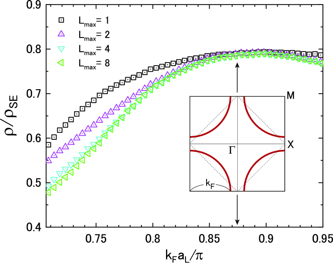
Figure 7: Umklapp factor of the resistivity for a circular Fermi-surface on a square lattice with $k_{F}{a_{L}}/\pi>1/\sqrt{2}$, where higher Umklapp vectors such as $(2\pi/{a_{L}},2\pi/{a_{L}})$ become players. The inset shows a circular Fermi-surface of radius $k_{F}\approx 0.874\pi/{a_{L}}$ centered at the M point, which corresponds to about 20% hole doping. Around this value of $k_{F}$, the convergence with respect to $L_{max}$ is fast and the Umklapp factor is nearly constant at about $0.78$.

In Fig. 5, we find that the convergence with respect to $L_{max}$ is slow. This is especially so around $k_{F}{a_{L}}/\pi=2-\sqrt{2}\approx 0.586$, where $\rho/\rho_{\rm SE}$ has a local minimum. But we have investigated this region more exhaustively with increased $L_{max}$ to assure that the value of the Umklapp factor there is about 0.2 but saturating at about 0.5 at large $k_{F}{a_{L}}$. If the Fermi-surface is large enough, so that higher Umklapp vectors $(2\pi/{a_{L}},2\pi/{a_{L}})$ become players and the true resistivity $\rho$ then becomes closer to $\rho_{\rm SE}$. For the about 20% hole doped cuprates near quantum-critical doping, the Fermi-surface is large. We have also calculated $\rho/\rho_{\rm SE}$ for $k_{F}{a_{L}}/\pi>1/\sqrt{2}$, where there is Umklapp scattering also for the next reciprocal vectors. As seen in Fig. 7, the convergence with respect to $L_{max}$ is fast and the Umklapp factor is nearly constant at about $0.78$ around $k_{F}{a_{L}}/\pi=2\sqrt{3/5\pi}\approx 0.874$, which corresponds to the radius of an oblate Fermi-surface centered at the M point of the 20% hole doped cuprates when approximated by a circle. We would therefore expect $0.5<\rho/\rho_{\rm SE}<1$. This is in line with the estimates given in [2] for the relative magnitude of the imaginary part of the self-energy in the diagonal direction, the coefficient of the $T\ln T$ specific heat and the resistivity scattering rate estimated from experiments.

In this context, the result in [57] is worth recalling; for $d>2$ where ${\hat{C}}_{N}$ is not a zero matrix, normal scattering also contributes to the electrical resistivity once Umklapp scattering is present. For transport theory in dimension $d\to\infty$ or for infinite number of neighbors, as in dynamical mean-field calculations, the Umklapp factor is identity, implying that the normal scattering contributes to the electrical resistivity as well as the Umklapp scattering. This should be equally true for the SYK-type models [74] in which $N$-sites are coupled to each other with $N\to\infty$.

II.6 Seebeck coefficient

The thermoelectric power $S$, also called the Seebeck coefficient, can be given using the transport coefficients $L_{ij}$,

$$S = \frac{L_{12}}{TL_{11}}.$$ (74)

In Sec. II-C, we have given an general expression of the off-diagonal transport coefficient $L_{12}=L_{21}$ at low temperatures [See Eq. (35)]. Here we consider $L_{12}$ and thus $S$ for the QXY-F model, where $L_{11}=\sigma$ is given by Eq. (59).

For the critical fluctuations and their coupling to fermions given by Eq. (42), $Y_{1}(t)$ in Sec. II-C can be obtained as

$$Y_{1}(t) = \frac{(-e)}{2\bar{g}^{2}N(0)T}\frac{{\tilde{v}}_{{\bf p}x}}{f(t)}\frac{1}{2}\,{\rm sech}\frac{t}{2}$$ (75)

$$-\frac{(-e)\langle{\tilde{v}}_{x}^{2}\rangle^{1/2}}{2\bar{g}^{2}N(0)T}\sum_{n=1}^{\infty}\varphi_{n,+}(t)\alpha_{n,1}$$

$$\times\frac{2}{N(0)}\int\frac{d{\bf q}}{(2\pi)^{d}}\delta({\tilde{\epsilon}}_{{\bf p}-{\bf q}})$$

$$\times\sum_{L}\bar{\psi}_{L}({\bf q})\left[\frac{1}{\lambda_{n,+}\hat{1}-\hat{B}}\right]_{L1},$$

where we have defined

$$\alpha_{n,1} \equiv \int_{-\infty}^{\infty}\varphi_{n,+}(x)\frac{1}{2}\,{\rm sech}\frac{x}{2}dx,$$ (76)

$$\bar{\psi}_{L}({\bf q}) \equiv \frac{\displaystyle{\sum_{\bf G}\int d{\bf k}\,\psi_{L}({\bf k})\delta({\tilde{\epsilon}}_{\bf k})\delta({\tilde{\epsilon}}_{{\bf k}+{\bf q}-{\bf G}})}}{\displaystyle{\sum_{{\bf G}^{\prime}}\int d{\bf k}^{\prime}\,\delta({\tilde{\epsilon}}_{{\bf k}^{\prime}})\delta({\tilde{\epsilon}}_{{\bf k}^{\prime}+{\bf q}-{\bf G}^{\prime}})}}.$$ (77)

Note that $Y_{1}(t)$ is a function of not only the dimensionless energy variable $t$ but also the momentum ${\bf p}$, which is not restricted on the Fermi-surface. For an ${\bf p}$ on the Fermi-surface, $Y_{1}(t)$ can be expanded in the Fermi-surface harmonics as $Y_{1}(t)=\sum_{L}\langle\psi_{L}|Y_{1}(t)\rangle\psi_{L}({\bf p})$ with

$$\langle\psi_{L}|Y_{1}(t)\rangle = \frac{(-e)\langle{\tilde{v}}_{x}^{2}\rangle^{1/2}}{2\bar{g}^{2}N(0)T}\sum_{n=1}^{\infty}\varphi_{n,+}(t)\alpha_{n,1}\left[\frac{\lambda_{n,+}}{\lambda_{n,+}\hat{1}-\hat{B}}\right]_{L1}.$$ (78)

Since the dc-electrical conductivity is given by $L_{11}=2\int_{-\infty}^{\infty}dt\sum_{L}\langle X_{1}(t)|\psi_{L}\rangle\langle\psi_{L}|Y_{1}(t)\rangle$ with $\langle X_{1}(t)|\psi_{L}\rangle=(-e)\langle{\tilde{v}}_{x}^{2}\rangle^{1/2}\alpha_{n,1}$, Eq. (78) immediately leads to Eq. (59). As seen in Sec. II-E, for a large Fermi-surface, the matrix ${\hat{B}}$ becomes small due to the frequent occurrence of Umklapp scattering. Note that substituting ${\hat{B}}={\hat{0}}$ into Eq. (78) and using $\sum_{n=1}^{\infty}\varphi_{n,+}(t)\alpha_{n,1}=(1/2)\,{\rm sech}(x/2)/f(t)$ reproduce the first term in Eq. (75) for any ${\bf p}$ on the Fermi-surface. Similarly, for such a large Fermi-surface, the second term (the vertex correction) is much smaller than the first term (the self-energy correction) in Eq. (75) for the ${\bf p}$ away from the Fermi-surface. However, for a small Fermi-surface without Umklapp scattering, the second term is important and leads to a divergent electrical conductivity. On the other hand, the vertex corrections to the thermal current vanish regardless of the size of the Fermi-surface, and then $Y_{2}(t)$ is simply given by the self-energy correction,

$$Y_{2}(t) = \frac{1}{2\bar{g}^{2}N(0)}\frac{{\tilde{v}}_{{\bf p}x}}{f(t)}\frac{t}{2}\,{\rm sech}\frac{t}{2},$$ (79)

which always leads to the finite thermal conductivity.

The off-diagonal transport coefficient can be obtained by substituting Eqs. (75) and  (79) into Eq. (35). Since the spectral function for the MFL can be approximated by $A({\bf p},\varepsilon)={\tilde{A}}_{\bf p}(a^{-1}\varepsilon)$ with

$${\tilde{A}}_{\bf p}(x)=\frac{1}{\pi}\frac{{\tilde{\Gamma}}}{(x-\tilde{\epsilon}_{\bf p})^{2}+{\tilde{\Gamma}}^{2}},$$ (80)

where $a^{-1}\propto|\ln T|$ and ${\tilde{\Gamma}}\propto T$ are independent of momentum, $A_{0}={\tilde{A}}_{\bf p}(0)\to\delta(\tilde{\epsilon}_{\bf p})$ for $T\to 0$ and the next order term can be written formally as $A_{1}(t)=a^{-1}Tt\,{\tilde{A}}_{\bf p}^{\,\prime}(0)$. Then we can derive ${\cal I}_{1}(t,t^{\prime})$ by applying this formal expansion to the spectral functions in Eq. (16). As a result, the inverse of the single-particle renormalization factor $a$ can be taken out, and the off-diagonal transport coefficient is given by

$$L_{12} = a^{-1}{\tilde{L}}_{12}.$$ (81)

Here ${\tilde{L}}_{12}$ does not include $a$, and some manipulations lead to

$${\tilde{L}}_{12} = -\frac{eT}{\bar{g}^{2}}\frac{1}{N(0)}\int\frac{d{\bf p}}{(2\pi)^{d}}{\tilde{v}}_{{\bf p}x}^{2}\,\delta^{\prime}(-\tilde{\epsilon}_{\bf p})+\frac{eT}{\bar{g}^{2}}\frac{N^{\prime}(0)}{N(0)}\frac{\langle{\tilde{v}}_{x}^{2}\rangle}{2}\sum_{n=1}^{\infty}\alpha_{n,2}\alpha_{n,1}\left[\frac{\lambda_{n,+}}{\lambda_{n,+}\hat{1}-\hat{B}}\right]_{11}$$ (82)

$$+\frac{2eT}{{\bar{g}^{2}}}\frac{2\langle{\tilde{v}}_{x}^{2}\rangle^{1/2}}{N(0)^{2}}\sum_{L}\int\frac{d{\bf q}d{\bf p}}{(2\pi)^{2d}}{\tilde{v}}_{{\bf p}x}\,\delta(\tilde{\epsilon}_{\bf p})\tilde{A}_{{\bf p}-{\bf q}}^{\,\prime}(0)\bar{\psi}_{L}({\bf q})\left[\frac{1}{\hat{1}-\hat{B}}\right]_{L1}$$

$$+\frac{eT}{\bar{g}^{2}}\frac{2\langle{\tilde{v}}_{x}^{2}\rangle^{1/2}}{N(0)^{2}}\int\frac{d{\bf q}d{\bf p}}{(2\pi)^{2d}}{\tilde{v}}_{{\bf p}x}\left[\,\tilde{A}_{{\bf p}}^{\,\prime}(0)\delta({\tilde{\epsilon}}_{{\bf p}-{\bf q}})-\delta(\tilde{\epsilon}_{\bf p})\tilde{A}_{{\bf p}-{\bf q}}^{\,\prime}(0)\right]$$

$$\times\sum_{n=1}^{\infty}\alpha_{n,2}\alpha_{n,1}\sum_{L}\bar{\psi}_{L}({\bf q})\left[\frac{1}{\lambda_{n,+}\hat{1}-\hat{B}}\right]_{L1},$$

where

$$\alpha_{n,2}\equiv\int_{-\infty}^{\infty}\varphi_{n,+}(t)\frac{t^{2}}{2}\,{\rm sech}\frac{t}{2}dt.$$ (83)

Now we extend the matrix ${\hat{B}}$ which represents the vertex corrections to the electric current as

$$\left[{\hat{B}}(x,y)\right]_{LL^{\prime}}=-\frac{2}{N(0)^{2}}\int\frac{d{\bf q}d{\bf p}}{(2\pi)^{2d}}\psi_{L}({\bf p})\tilde{A}_{{\bf p}}(x)\tilde{A}_{{\bf p}-{\bf q}}(y)\bar{\psi}_{L^{\prime}}({\bf q}).$$ (84)

Then ${\hat{B}}={\hat{B}}(0,0)$ for $T\to 0$. Introducing the partial derivatives of ${\hat{B}}(x,y)$ at $x=0$ and $y=0$ as ${\hat{B}}_{x}\equiv\partial{\hat{B}}(x,0)/\partial x|_{x=0}$ and ${\hat{B}}_{y}\equiv\partial{\hat{B}}(0,y)/\partial y|_{y=0}$, we can write Eq. (82) as a rather compact form,

$${\tilde{L}}_{12} = -\frac{e\langle{\tilde{v}}_{x}^{2}\rangle T}{\bar{g}^{2}}\left(\frac{\langle{\tilde{m}}_{xx}^{-1}\rangle}{\langle{\tilde{v}}_{x}^{2}\rangle}-\frac{1}{2}\frac{N^{\prime}(0)}{N(0)}\right)-\frac{2e\langle{\tilde{v}}_{x}^{2}\rangle T}{{\bar{g}^{2}}}\left[{\hat{B}}_{y}(\hat{1}-\hat{B})^{-1}\right]_{11}$$ (85)

$$+\frac{e\langle{\tilde{v}}_{x}^{2}\rangle T}{\bar{g}^{2}}\sum_{n=1}^{\infty}\alpha_{n,2}\alpha_{n,1}\left[\left(\frac{1}{2}\frac{N^{\prime}(0)}{N(0)}\hat{B}-{\hat{B}}_{x}+{\hat{B}}_{y}\right)(\lambda_{n,+}\hat{1}-\hat{B})^{-1}\right]_{11},$$

where the average of the inverse mass tenser over the Fermi-surface is given by

$$\langle{\tilde{m}}_{xx}^{-1}\rangle=\frac{1}{N(0)}\int\frac{d{\bf p}}{(2\pi)^{d}}\frac{\partial{\tilde{v}}_{{\bf p}x}}{\partial p_{x}}\,\delta(\tilde{\epsilon}_{\bf p}).$$ (86)

Since the renormalization factor $a$ does not appear in ${\tilde{L}_{12}}$ and in $L_{11}$, the Seebeck coefficient $S=a^{-1}\tilde{L}_{12}/L_{11}T$ is proportional to $a^{-1}$. In the case of the large Fermi-surface as in the cuprates near quantum critical doping, Umklapp scattering is expected to make the vertex corrections ineffective for $L_{12}$ as well as for the electrical conductivity $L_{11}$. Then the first term can be dominant in Eq. (85), leading to

$$\frac{S}{T} \simeq -\frac{2\pi^{2}}{7\zeta(3)}\frac{a^{-1}}{e}\left(\frac{\langle{\tilde{m}}_{xx}^{-1}\rangle}{\langle{\tilde{v}}_{x}^{2}\rangle}-\frac{1}{2}\frac{N^{\prime}(0)}{N(0)}\right).$$ (87)

As found in experiments in the heavy fermion systems [75] and in cuprates [16, 17, 18] as well as the Fe-based compounds [19], the magnitude of the Seebeck coefficient $S$ is proportional to $\propto a^{-1}T\propto T|\ln\frac{\omega_{c}}{T}|$, i.e. to the electronic specific heat. $\omega_{c}$ is the upper cut-off in the fluctuation spectra and may be obtained by fit to measured $S$, which is often easier to measure than the specific heat. The sign of $S$ requires more detailed information about the electron dispersion, such as the inverse mass tensor and the energy dependence of the density of states. We remind again of the absence of the logarithmic mass enhancement in resistivity and in thermal conductivity. Note also that unlike the case of thermal conductivity, there are no symmetry reasons that the vertex renormalization is absent in the Seebeck coefficient. Our result of the presence of the logarithmic mass enhancement in the Seebeck coefficient is for an ideal system without impurities, although a similar enhancement factor also appears due to impurity scattering [76].

III Conclusions

It has been apparent for quite some time now that the remarkably simple and universal properties near quantum-criticality of a large number of quasi-2-dimensional systems may only be explained through the $\omega/T$ scaling of critical fluctuations proposed in 1989. Such a spectra was derived for the QXY-F model. Although some properties like the single-particle spectra and the specific heat are very easy to calculate, the calculation of the transport properties is more subtle and to be completely convincing requires a technical and detailed calculation. The physical principles and conservation laws underlying these transport properties and the calculations have been performed and explained in this paper.

We have solved the integral equation for the vertex coupling to external fields in the Kubo expression for electrical and thermal conductivities and the Seebeck coefficient, using scattering of fermions from the known propagator for the quantum fluctuations of the QXY-F model. We have derived exact results at low temperatures for transport properties and shown explicitly that the linear in temperature electrical resistivity results from Umklapp scattering, whereas the thermal conductivity of electrons is a temperature-independent constant that is finite due to normal scattering, reflecting different effects of the Planckian dissipation on charge and energy currents. This has been possible only because of the simplicity and the unusual nature of the scale-invariant spectra of fluctuations. The simplicity is due to the fact that the fluctuations are due to two orthogonal topological objects, one fluctuating only in space and the other only in time, and the fact that fermions couple only to gradients in space or time of the phase variable in the xy model. This model has direct applicability to a variety of physical problems of experimental interest which give experimental results with linear in $T$ and linear in $H$ resistivity, temperature-independent thermal conductivity and $T\ln(\omega_{c}/T)$ specific heat, with coefficients which are simply related to each other. This is also the only example of a physically applicable model we know for which the Kubo equation for transport has been solved. The general theory presented should be of considerable technical interest although in the specific problem solved it provides corrections only by a factor of about $3/4$ for Fermi-surfaces of interest in electrical resistivity and none for thermal conductivity to the simpler calculations done earlier. Among the several new results derived here are the presence of the logarithmic in temperature mass enhancement in the leading term in the Seebeck coefficient and its absence in the thermal conductivity. There is a vast list of experiments which are explained unambiguously through this work but the absence of the mass enhancement of the specific heat in the thermal conductivity is yet to be tested. Although all calculations in this paper are for an ideal system without impurities, it is an interesting and important question what impurities do to quantum criticality [77, 78]. For more detailed comparisons with experiments, it would be necessary to generalize the theory to include impurity scattering.

We hope that this work, through its exact results and their quantitative agreement with experiments, provides an unambiguous understanding of the universality of the ”strange metal” anomalies near quantum-critical points discovered in experiments in a variety of different materials with quite different order parameters. These include the cuprates with loop-current order without breaking translation symmetry, planar antiferromagnets and incommensurate Ising antiferromagnets, TBG if it indeed has loop-current order breaking translation symmetry, as well as TBWSe. We have emphasized that the reason for the universality near quantum-criticality is that they are all described by the QXY-F model. It follows also that the superconductivity in them is promoted by scattering of fermions from the same fluctuations which give the normal state strange metal anomalies.

Acknowledgements:  HM is grateful to M. Ogata and H. Matsuura for fruitful discussions. CMV wishes to acknowledge several discussions and email exchanges with Dominic Else and Senthil Todadri which were useful in understanding their work. The work of HM was partly supported by Grants-in-Aid for Scientific Research from the Japan Society for the Promotion of Science (Grant Nos. JP21K03426, JP18K03482, and JP18H01162) and JST-Mirai Program, Japan (Grant No. JPMJMI19A1). CMV wishes to thank James Analytis, Robert Birgeneau and Joel Moore for arranging for him to be a ”re-called Professor” at the Physics department of University of California, Berkeley, where part of this work was done and to Aspen Center for Physics where part of this work was done last summer. Aspen Center for Physics is partially supported by the National Science Foundation of USA through grant PHY-1607611.

IV Appendices

IV.1 Summary of the critical fluctuations of quantum xy model coupled to fermions

The quantum xy model in 2+1 dimensions is defined in terms of the action $S_{qxy}$ of a rotor of fixed length and angle $\theta({\bf x},\tau)$ at a point ${\bf x}$ and imaginary time $\tau$, which is periodic in the inverse temperature $(0,\beta)$, is given by the following action:

$$S_{qxy} = -K_{0}\sum_{\langle{\bf x,x}^{\prime}\rangle}\int_{0}^{\beta}d\tau\cos(\theta_{{\bf x},\tau}-\theta_{{\bf x}^{\prime},\tau})$$ (88)

$$+ \frac{1}{2E_{c}}\sum_{{\bf x}}\int_{0}^{\beta}d\tau\left(\frac{d\theta_{{\bf x}}}{d\tau}\right)^{2}.$$

The variable $\theta$ refers to different quantities in different physical situation. It refers to the direction of the anapole vector in the loop-current order in cuprates [23], to the in-plane anti-ferromagnetic order-vector in some heavy-fermion, transformed on a bi-partite lattice into a model coupled ferromagnetically in the plane [26, 27], or to the phase of an incommensurate antiferro-magnetic Ising order in another heavy-fermion [26, 27]. If the lattice anisotropy is more than 4-fold, it is irrelevant in the quantum model and is ignored. Recently, it has been suggested [28] that the loop-current order proposed in Moiré TBG [46, 47], (which is remarkably similar to an order presented for graphene due to nearest neighbor interactions [79]), and proposed in TBWSe also fall in the quantum-xy class.

The model of Eq. (88) has only Lorentz-invariant fluctuations at long wave-lengths, which are inadequate to address questions in problems with fermions. It must be coupled to fermions to give interesting results. $\theta({\bf x},\tau)$ is not gauge invariant and cannot couple to any physical variable. $\nabla\theta({\bf x},\tau)$ is proportional to a collective mode current, and if $\theta$ refers to the direction of a vector which is time-reversal and inversion-odd, it can couple to the fermion current. The conjugate variable in the quantum-rotor problem, i.e. the angular momentum $\frac{d\theta({\bf x},\tau)}{d\tau}$ which is proportional to the orbital magnetic moment or in a Hamiltonian formulation ${\bf L}_{z}({\bf x},\tau)$ similarly couples to the local fermion angular momentum, which is proportional to the fermion orbital moment. After integrating over the fermions (which can be done formally in terms of the fermion current-current correlation function), both of these give contributions of the same functional form to the Lagrangian. This form is of the Caldeira-Leggett type although the physics used to derive it is different. It is

$$S_{c-f}=\frac{\alpha}{4\pi^{2}}\sum_{\langle{\bf x,x}^{\prime}\rangle}\int d\tau d\tau^{\prime}\frac{\pi^{2}}{\beta^{2}}\frac{\left[(\theta_{{\bf x},\tau}-\theta_{{\bf x}^{\prime},\tau})-(\theta_{{\bf x},\tau^{\prime}}-\theta_{{\bf x}^{\prime},\tau^{\prime}})\right]^{2}}{\sin^{2}\left(\frac{\pi|\tau-\tau^{\prime}|}{\beta}\right)}$$ (89)

Note that the square bracket in the integrand is the sum of the discrete version of both $\nabla\theta({\bf r},\tau)$ and $\frac{d\theta({\bf r},\tau)}{d\tau}$. Eq. (89) looks complicated but it looks much simpler when expressed as a function of real frequency $\omega$ and momentum $q$: $\frac{\alpha}{4\pi^{2}}|\omega|q^{2}|\theta({\bf q},\omega)|^{2}.$ $\alpha$ is the conductivity of the fermions in the limit $q\to 0,\omega\to 0,T\to 0$ made dimensionless in terms of $e^{2}/h$. One could also couple to $\cos(\theta({\bf x},\tau))$. This has also been investigated [31] and is found to be irrelevant.

The QXY-F model which has been investigated by quantum-Monte-carlo exhaustively is given by

$$S_{qxy-F}\equiv S_{qxy}+S_{c-f}.$$ (90)

As a function of $K_{0},E_{c}$ and $\alpha$ has three different lines of transitions. We will be interested in the problem under discussion where the quantum-critical point fluctuations are at the transition in which $\cos(\theta({\bf x},\tau))$ orders both in space and time. The most important quantity to calculate, which is directly relevant to the calculation of the properties of fermions is the correlation function of the fluctuations

$$D({\bf r},\tau)\equiv<e^{-i\theta({\bf r},\tau)}e^{i\theta(0,0)}>\propto<L_{z}({\bf r},\tau)L_{z}(0,0)>$$ (91)

The proportionality of the fluctuations of the angular momentum variable to those of $e^{i\theta}$ has been shown [80]. The result for the fluctuations are very accurately given by [30, 31, 81]

$$D({\bf r},\tau)=D_{0}\frac{\tau_{c}^{2}}{\tau}~{}e^{-(\tau/\xi_{\tau})^{1/2}}~{}\ln(r/a_{L})e^{-r/\xi_{r}}.$$ (92)

$D_{0}$ provides the magnitude of the fluctuations which is given by the square magnitude of the orbital current moments per unit-cell. $\tau_{c}^{-1}$ is the ultraviolet energy cut-off and $a_{L}$ is the lattice constant. Further the spatial correlation $\xi_{r}$ is negligible for all practical purposes compared to the temporal correlation length:

$$\xi_{r}/a_{L}=\ln(\xi_{\tau}/\tau_{c}).$$ (93)

The most remarkable feature of (92) is that they are of product form in time and space. This arises because of the nature of the two kinds of orthogonal topological excitations responsible for the correlation functions noted in [25, 58] one of which propagates only in space and the other only in time.

An example of the accuracy of the extensive calculations [30, 31] from which the above conclusions are drawn is given by Fig. 8.

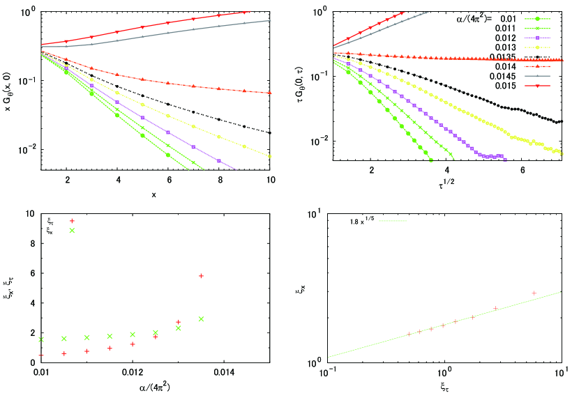
Figure 8: This figure gives an example of the correlation function $D({\bf x},\tau)$ (called $G$ in the original paper), calculated in [31]. All results are for fixed $K_{0}$ and $E_{c}$ and varying $\alpha/4\pi^{2}$. Top left at small $\tau$ $D$ is shown as a function of $x$, while top-right shows it at small $x$ as a function of $\tau$. With such fixed values, there is a critical point for $\alpha/4\pi^{2}=0.014\pm.0002$. These curves can be collapsed and shown to be of a scaling form near the critical form from which the correlation length in time $\xi_{\tau}$ and in space $\xi_{x}$ can be deduced as shown at bottom left. In bottom right, the relation between $\xi_{\tau}$ and $\xi_{x}$ is shown to be $\xi_{x}\sim\xi_{\tau}^{1/z}$. The minimum value of $z$ with which these results can be fit is $6$ but $z\to\infty$, i.e. $\xi_{x}\sim\log\xi_{\tau}$ fits very well.

Analytic RG calculations on the model:

After making the Villain transformation, the model given by Eq. (90) for $S_{qxy-F}$ is harmonic in $\theta$. Integrating over such spin-wave like fluctuations, as is done for the classical xy model, leaves a model for topological excitations only [25, 58, 29]. A particular choice of the degrees of freedom exactly transforms the resulting Lagrangian into a remarkably simple form and provides crucial insight to the Monte-carlo results. The choice consists in defining two varieties of topological charges through the effective integer velocity field ${\bf m}({\bf r},\tau)$ on sites of the space-time lattice. ${\bf m}({\bf r},\tau)$ has both a transverse and a longitudinal part

$${\bf m}({\bf r},\tau) = {\bf m}_{t}({\bf r},\tau)+{\bf m}_{\ell}({\bf r},\tau),$$ (94)

$$\nabla\cdot{\bf m}_{t} = 0,~{}\nabla\times{\bf m}_{\ell}=0.$$ (95)

Quantized topological charges for vortices $\rho_{v}$ and for warps $\rho_{w}$ are defined by

$$\nabla\times{\bf m}_{t}({\bf r},\tau) = \rho_{v}({\bf r},\tau),$$ (96)

$$\frac{d}{d\tau}\big{(}\nabla\cdot{\bf m}_{\ell}\big{)} = \rho_{w}({\bf r},\tau).$$ (97)

$\rho_{v}$ and $\rho_{w}$ are orthogonal fields. In terms of them $S_{qxy-F}$ to be re-written as

$$S_{qxy-F} = S_{v}+S_{w}+S_{w}^{\prime},$$ (98)

$$S_{v} = \frac{J}{2\pi}\sum_{i\neq j}\rho_{v}({r}_{i},\tau_{i})\ln\frac{|{r}_{i}-{r}_{j}|}{a_{c}}\rho_{v}({r}_{j},\tau_{i})+\ln y_{v}\sum_{i}|\rho_{v}({r}_{i},\tau_{i})|^{2}$$ (99)

$$S_{w} = \alpha\sum_{i\neq j}\rho_{w}({r}_{i},\tau_{i})\ln\frac{|\tau_{i}-\tau_{j}|}{\tau_{c}}\rho_{w}({r}_{i},\tau_{j})+\ln y_{w}\sum_{i}|\rho_{w}({r}_{i},\tau_{i})|^{2}.$$ (100)

$$S_{w}^{\prime} = g\sum_{i\neq j}\rho_{w}({r}_{i},\tau_{i})\frac{1}{\sqrt{|{r}_{i}-{r}_{j}|^{2}+v^{2}(\tau_{i}-\tau_{j})^{2}}}\rho_{w}({r}_{j},\tau_{j})$$ (101)

$S_{v}$ is the action of vortices which interact logarithmically in space but is local in time. $S_{w}$ is the action of warps which interact logarithmically in time but is local in space. $y_{v}$ and the $y_{w}$ are the fugacities of the vortices and warps respectively. The last term $S_{w}^{\prime}$ effectively couples the vortices and warps through $g$ and controls which of the two dominates the correlations to determine the correlation functions. This is done through the flow of $v^{2}$ under renormalization, which is equivalent to the flow of the dynamical critical exponent $z$. In most of the range of parameters, warps dominate the order and force the order of vortices. Only results in this range have been quoted here. Direct evidence for warps and vortices is observed in the quantum-monte-carlo calculations and their correlations can be related to the fluctuations given by the order-parameter fluctuations defined by Eq. (91)

The transformed problem in terms of two kinds of topological excitations is as well soluble as the Kosterlitz solution [82, 83] of the classical xy model in first order RG. The first order RG solution reproduces essentially all but not all features of the Monte-Carlo solution.

A remarkable result from Monte-carlo is that at the critical point with varying dimensionless ratios $K_{0}E_{c},\alpha$, not only are the correlation functions of the same form but the amplitude $D_{0}$ is also independent of them. This is not reproduced by the one loop RG, nor is the fact that the correlation decays as $e^{-(\tau/\xi_{\tau})^{1/2}}$ and not as $e^{-(\tau/\xi_{\tau})}$.

The correlation function calculated by RG can be continued to real frequency and momentum only numerically for finite correlation lengths. The results can be well fitted to the form given by the analytical calculations:

$$D({\bf q},\omega)=D_{0}\Big{(}\ln\big{|}\frac{\omega_{c}}{max(\omega,\pi T)}\big{|}-i\tanh\frac{\omega}{\sqrt{(2T)^{2}+\xi_{\tau}^{-2}}}\Big{)}\frac{\xi_{r}^{-2}}{q^{2}+\xi_{r}^{-2}}.$$ (102)

The relation in Eq. (93) makes the problem effectively spatially local. Moreover the coupling to the fermions of the fluctuations comes from the coupling of their current to the fermion current and of their angular momentum to the fermion angular momentum [84, 85]. These couplings are the same that are used in generating Eq. (89) for $S_{cf}$. Both of these lead to a vertex coupling to fermions

$$g({\bf q})=g_{0}q^{2}.$$ (103)

where ${\bf q}$ is the momentum transfer. Eqs. (102) and (103) have been used to calculate the fermion self-energy. The wiggly lines in all the figures in the text refers to (102).

IV.2 Landau-Boltzmann transport equations

For Landau Fermi-liquids or MFL, the single-particle spectral function is approximated by

$$A({\bf p},\varepsilon)\approx a_{\bf p}\delta(\varepsilon-\epsilon_{\bf p}^{*}),$$ (104)

where $\epsilon_{\bf p}^{*}=a_{\bf p}{\tilde{\epsilon}}_{\bf p}$ is the energy of the quasi-particle. Even though in MFL the quasi-particle weight $a_{\bf p}$ is non-zero only due to a logarithmic factor, a Fermi-surface is well defined so that for low temperatures we can use Eq. (104) without introducing errors, where all the effects of $a_{\bf p}$ are canceled out in the theory such that $A({\bf p},0)=a_{\bf p}\delta(\epsilon_{\bf p}^{*})=\delta({\tilde{\epsilon}}_{\bf p})$. (It is important to note that this cancellation occurs also for the MFL, where $a_{\bf p}(\epsilon_{\bf p}^{*})\to 0$, as $|1/\ln(\epsilon_{\bf p}^{*})|$.) Hence, the low-temperature conductivity can be obtained without using the Fermi-liquid assumption, Eq. (104), and the results given by Eqs. (36) and (37) do not include any quasi-particle weight. However, Landau theory gives a familiar physical picture of quasiparticles carrying electric and thermal currents, so here we derive the Landau-Boltzmann transport equations for a model of fermions on a lattice scattering with collective fluctuations.

Substituting Eq. (104) into Eq. (20), we get

$$v_{{\bf p}x}^{*}\,{\rm sech}\frac{\epsilon_{\bf p}^{*}}{2T} = \frac{1}{2}\int\frac{d{\bf p}^{\prime}d{\bf k}d{\bf k}^{\prime}}{(2\pi)^{2d}}S({\bf p},{\bf k};{\bf p}^{\prime},{\bf k}^{\prime})\,{\rm sech}\frac{\epsilon_{{\bf p}^{\prime}}^{*}}{2T}\,{\rm sech}\frac{\epsilon_{\bf k}^{*}}{2T}\,{\rm sech}\frac{\epsilon_{{\bf k}^{\prime}}^{*}}{2T}$$ (105)

$$\times\big{[}\Phi({\bf p})-\Phi({\bf p}^{\prime})+\Phi({\bf k})-\Phi({\bf k}^{\prime})\big{]},$$

where $v_{{\bf p}x}^{*}=a_{\bf p}{\tilde{v}}_{x}({\bf p},\epsilon_{\bf p}^{*})$ and $\Phi({\bf p})=\Phi({\bf p},\epsilon_{\bf p}^{*})$, and

$$S({\bf p},{\bf k};{\bf p}^{\prime},{\bf k}^{\prime}) = 2\pi W({\bf p}-{\bf p}^{\prime},\epsilon_{\bf p}^{*}-\epsilon_{{\bf p}^{\prime}}^{*})a_{\bf p}a_{{\bf p}^{\prime}}a_{\bf k}a_{{\bf k}^{\prime}}$$ (106)

$$\times\Delta^{d}({\bf p}-{\bf p}^{\prime}+{\bf k}-{\bf k}^{\prime})\delta(\epsilon_{\bf p}^{*}-\epsilon_{{\bf p}^{\prime}}^{*}+\epsilon_{\bf k}^{*}-\epsilon_{{\bf k}^{\prime}}^{*}).$$

Noting that

$$f(\varepsilon)\bar{f}(\varepsilon^{\prime})f(\varepsilon_{1})\bar{f}(\varepsilon-\varepsilon^{\prime}+\varepsilon_{1})=\frac{1}{16}{\rm sech}\frac{\varepsilon}{2T}\,{\rm sech}\frac{\varepsilon^{\prime}}{2T}\,{\rm sech}\frac{\varepsilon_{1}}{2T}\,{\rm sech}\frac{\varepsilon-\varepsilon^{\prime}+\varepsilon_{1}}{2T},$$ (107)

where $\bar{f}(\varepsilon)=1-f(\varepsilon)$, we can write Eq. (105) in the familiar form of the Landau-Boltzmann transport equation for the velocity distribution function $\Phi({\bf p})$ as

$$v_{{\bf p}x}^{*}\left(-\frac{\partial f(\epsilon_{\bf p}^{*})}{\partial\epsilon_{\bf p}^{*}}\right) = \frac{2}{T}\int\frac{d{\bf p}^{\prime}d{\bf k}d{\bf k}^{\prime}}{(2\pi)^{2d}}S({\bf p},{\bf k};{\bf p}^{\prime},{\bf k}^{\prime})f(\epsilon_{\bf p}^{*})\bar{f}(\epsilon_{{\bf p}^{\prime}}^{*})f(\epsilon_{\bf k}^{*})\bar{f}(\epsilon_{{\bf k}^{\prime}}^{*})$$ (108)

$$\times\big{[}\Phi({\bf p})-\Phi({\bf p}^{\prime})+\Phi({\bf k})-\Phi({\bf k}^{\prime})\big{]}.$$

[From Eq. (32), that for the thermal-current distribution function is given by replacing $v_{{\bf p}x}^{*}$ with $v_{{\bf p}x}^{*}\epsilon_{\bf p}^{*}$.] It should be noted, however, that for fermions scattering with collective fluctuations, $W$ in $S$ is given by Eq. (19).

By substituting Eq. (104) for Eq. (14), Eq. (3) is re-derived as

$$\sigma(\omega,T)=2e^{2}\int\frac{d{\bf p}}{(2\pi)^{d}}\left(-\frac{\partial f(\epsilon_{\bf p}^{*})}{\partial\epsilon_{\bf p}^{*}}\right)v_{{\bf p}x}^{*}\Phi({\bf p},\omega).$$ (109)

From Eqs. (15) and (108), $\Phi({\bf p},\omega)$ then satisfies

$$v_{{\bf p}x}^{*}\left(-\frac{\partial f(\epsilon_{\bf p}^{*})}{\partial\epsilon_{\bf p}^{*}}\right) = -i\omega\left(-\frac{\partial f(\epsilon_{\bf p}^{*})}{\partial\epsilon_{\bf p}^{*}}\right)\left[\Phi({\bf p},\omega)-\int\frac{d{\bf p}^{\prime}}{(2\pi)^{d}}g({\bf p},{\bf p}^{\prime})\left(-\frac{\partial f(\epsilon_{{\bf p}^{\prime}}^{*})}{\partial\epsilon_{{\bf p}^{\prime}}^{*}}\right)\Phi({\bf p}^{\prime},\omega)\right]$$ (110)

$$+\frac{2}{T}\int\frac{d{\bf p}^{\prime}d{\bf k}d{\bf k}^{\prime}}{(2\pi)^{2d}}S({\bf p},{\bf k};{\bf p}^{\prime},{\bf k}^{\prime})f(\epsilon_{\bf p}^{*})\bar{f}(\epsilon_{{\bf p}^{\prime}}^{*})f(\epsilon_{\bf k}^{*})\bar{f}(\epsilon_{{\bf k}^{\prime}}^{*})$$

$$\times\big{[}\Phi({\bf p},\omega)-\Phi({\bf p}^{\prime},\omega)+\Phi({\bf k},\omega)-\Phi({\bf k}^{\prime},\omega)\big{]},$$

where $g({\bf p},{\bf p}^{\prime})=a_{\bf p}\Gamma^{k}({\bf p},\epsilon_{\bf p}^{*},{\bf p}^{\prime},\epsilon_{{\bf p}^{\prime}}^{*})a_{{\bf p}^{\prime}}$.

IV.3 Umklapp vertex for a circular Fermi-surface

From Eq. (48) with use of $\psi_{L}(-{\bf p})=-\psi_{L}({\bf p})$, the matrix elements of $\hat{C}=\hat{1}-\hat{B}$ are obtained as

$$C_{LL^{\prime}} = \frac{1}{N(0)^{2}}\int\frac{d{\bf p}d{\bf p}^{\prime}}{(2\pi)^{2d}}\psi_{L}({\bf p})\delta({\tilde{\epsilon}}_{\bf p})\delta({\tilde{\epsilon}}_{{\bf p}^{\prime}})$$ (111)

$$\times\int\frac{d{\bf k}d{\bf k}^{\prime}}{(2\pi)^{d}}\Delta^{d}({\bf p}-{\bf p}^{\prime}+{\bf k}-{\bf k}^{\prime})\delta({\tilde{\epsilon}}_{\bf k})\delta({\tilde{\epsilon}}_{{\bf k}^{\prime}})$$

$$\times\left[\psi_{L^{\prime}}({\bf p})-\psi_{L^{\prime}}({\bf p}^{\prime})+\psi_{L^{\prime}}({\bf k})-\psi_{L^{\prime}}({\bf k}^{\prime})\right]$$

$$\times\left[\int\frac{d{\bf k}_{1}d{\bf k}_{1}^{\prime}}{(2\pi)^{d}}\Delta^{d}({\bf p}-{\bf p}^{\prime}+{\bf k}_{1}-{\bf k}_{1}^{\prime})\delta({\tilde{\epsilon}}_{{\bf k}_{1}})\delta({\tilde{\epsilon}}_{{\bf k}_{1}^{\prime}})\right]^{-1}.$$

Since $\Delta^{d}({\bf p}-{\bf p}^{\prime}+{\bf k}-{\bf k}^{\prime})=\sum_{\bf G}\delta^{d}({\bf p}-{\bf p}^{\prime}+{\bf k}-{\bf k}^{\prime}-{\bf G})$, the matrix can be separated as $\hat{C}=\hat{C}_{N}+\hat{C}_{U}$, where $\hat{C}_{N}$ and $\hat{C}_{U}$ are the contributions from normal (${\bf G}={\bf 0}$) and Umklapp (${\bf G}\neq{\bf 0}$) scatterings, respectively. $\hat{C}_{N}$ has a zero eigenvalue corresponding to conservation of crystal momentum; in three dimensions it is generally a nonzero matrix. However, two dimensions are special. Consider, for example, the circular Fermi-surface shown in Fig. 9(a). For the given ${\bf p}$ and ${\bf p}^{\prime}$, there are only two possible processes for which ${\bf p}$, ${\bf p}^{\prime}$, ${\bf k}$, and ${\bf k}^{\prime}$ are on the Fermi-surface and ${\bf p}+{\bf k}={\bf p}^{\prime}+{\bf k}^{\prime}$; one process is described by ${\bf k}=-{\bf p}$ and ${\bf k}^{\prime}=-{\bf p}^{\prime}$, the other by ${\bf k}={\bf p}^{\prime}$ and ${\bf k}^{\prime}={\bf p}$. Since $\psi_{L^{\prime}}({\bf p})-\psi_{L^{\prime}}({\bf p}^{\prime})+\psi_{L^{\prime}}({\bf k})-\psi_{L^{\prime}}({\bf k}^{\prime})=0$ in Eq. (111) for the both processes, $\hat{C}_{N}$ is a zero matrix. As discussed in [57], this result holds broadly for noncircular Fermi-surfaces on a two-dimensional lattice, where ${\hat{C}}={\hat{C}}_{U}$.

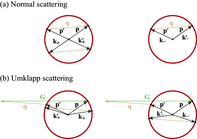
Figure 9: Normal and Umklapp scattering processes for a two-dimensional circular Fermi-surface. For the given ${\bf p}$, ${\bf p}^{\prime}$, and ${\bf G}$, there are only two processes that satisfy ${\bf p}-{\bf p}^{\prime}+{\bf k}-{\bf k}^{\prime}={\bf G}$, indicated by $\pm$. These processes are related by ${\bf k}_{\pm}^{\prime}=-{\bf k}_{\mp}$. (a) For normal scattering (${\bf G}={\bf 0}$), ${\bf k}_{+}=-{\bf p}$, ${\bf k}_{+}^{\prime}=-{\bf p}^{\prime}$, ${\bf k}_{-}={\bf p}^{\prime}$ and ${\bf k}_{-}^{\prime}={\bf p}$, so that $\psi_{L^{\prime}}({\bf p})-\psi_{L^{\prime}}({\bf p}^{\prime})+\psi_{L^{\prime}}({\bf k}_{\pm})-\psi_{L^{\prime}}({\bf k}_{\pm}^{\prime})$ in Eq. (111) is identically zero. (b) For Umklapp scattering (${\bf G}\neq{\bf 0}$), $\psi_{L^{\prime}}({\bf k}_{+})-\psi_{L^{\prime}}({\bf k}_{+}^{\prime})=\psi_{L^{\prime}}({\bf k}_{-})-\psi_{L^{\prime}}({\bf k}_{-}^{\prime})$ but $\psi_{L^{\prime}}({\bf p})-\psi_{L^{\prime}}({\bf p}^{\prime})+\psi_{L^{\prime}}({\bf k}_{\pm})-\psi_{L^{\prime}}({\bf k}_{\pm}^{\prime})$ becomes nonzero.

Let us consider in more detail $\hat{C}$ for a two-dimensional circular Fermi-surface with a Fermi wavenumber $k_{F}$. As shown in Fig. 9, for the given ${\bf p}$, ${\bf p}^{\prime}$, and ${\bf G}$ (we include normal processes by ${\bf G}={\bf 0}$), the two possible sets of solutions satisfying ${\bf p}-{\bf p}^{\prime}+{\bf k}-{\bf k}^{\prime}={\bf G}$ for ${\bf p}$, ${\bf p}^{\prime}$, ${\bf k}$, and ${\bf k}^{\prime}$ on the Fermi-surface is given by $({\bf k},{\bf k}^{\prime})=({\bf k}_{\pm},{\bf k}_{\pm}^{\prime})$. These solutions are explicitly given by

$$k_{\pm,x}^{\prime} = -k_{\mp,x}=\frac{q_{x}}{2}\pm\frac{q_{y}}{2}\sqrt{\frac{4k_{F}^{2}}{q^{2}}-1},$$ (112)

$$k_{\pm,y}^{\prime} = -k_{\mp,y}=\frac{q_{y}}{2}\mp\frac{q_{x}}{2}\sqrt{\frac{4k_{F}^{2}}{q^{2}}-1},$$ (113)

where ${\bf q}={\bf p}-{\bf p}^{\prime}-{\bf G}$. Let $\theta$ and $\theta^{\prime}$ be the angles of ${\bf p}$ and ${\bf p}^{\prime}$, respectively. Then, depending on the reciprocal vector ${\bf G}=(G_{x},G_{y})$, the angles $\alpha_{\pm}$ of ${\bf k}_{\pm}^{\prime}$, which are functions of $\theta$ and $\theta^{\prime}$, is obtained through

$$\cos\alpha_{\pm}(\theta,\theta^{\prime};{\bf G}) = \frac{1}{2}\left(\cos\theta-\cos\theta^{\prime}-\frac{G_{x}}{k_{F}}\right)$$ (114)

$$\pm\frac{1}{2}\left(\sin\theta-\sin\theta^{\prime}-\frac{G_{y}}{k_{F}}\right)\frac{\sqrt{1-X^{2}(\theta,\theta^{\prime};{\bf G})}}{X(\theta,\theta^{\prime};{\bf G})},$$

$$\sin\alpha_{\pm}(\theta,\theta^{\prime};{\bf G}) = \frac{1}{2}\left(\sin\theta-\sin\theta^{\prime}-\frac{G_{y}}{k_{F}}\right)$$ (115)

$$\mp\frac{1}{2}\left(\cos\theta-\cos\theta^{\prime}-\frac{G_{x}}{k_{F}}\right)\frac{\sqrt{1-X^{2}(\theta,\theta^{\prime};{\bf G})}}{X(\theta,\theta^{\prime};{\bf G})},$$

where

$$X(\theta,\theta^{\prime};{\bf G})=\frac{1}{2}\sqrt{\left(\cos\theta-\cos\theta^{\prime}-\frac{G_{x}}{k_{F}}\right)^{2}+\left(\sin\theta-\sin\theta^{\prime}-\frac{G_{y}}{k_{F}}\right)^{2}}.$$ (116)

The average over the Fermi-surface is given by

$$\frac{1}{N(0)}\int\frac{d{\bf p}}{(2\pi)^{2}}\delta({\tilde{\epsilon}}_{{\bf p}})=\int_{-\pi}^{\pi}\frac{d\theta}{2\pi},$$ (117)

where ${\tilde{\epsilon}}_{{\bf p}}=(p^{2}-k_{F}^{2})/2{\tilde{m}}$ and $N(0)={\tilde{m}}/2\pi$, but the effect of the mass ${\tilde{m}}$ is canceled in $\hat{C}$. The Fermi-surface harmonics $\psi_{L}({\bf p})$ are given by

$$\psi_{L}({\bf p})=\sqrt{2}\cos(2L-1)\theta,$$ (118)

where the $L=1$ Fermi-surface harmonics is proportional to the $x$ component of the velocity or the momentum, $\psi_{1}({\bf p})=\sqrt{2}\cos\theta=\sqrt{2}p_{x}/k_{F}$. Therefore we obtain the matrix elements of $\hat{C}$ for the two-dimensional circular Fermi-surface as

$$C_{LL^{\prime}} = 2\sum_{{\bf G}\neq{\bf 0}}\int_{-\pi}^{\pi}\frac{d\theta d\theta^{\prime}}{(2\pi)^{2}}w(\theta,\theta^{\prime};{\bf G})\cos\{(2L-1)\theta\}$$ (119)

$$\times\left[\cos\{(2L^{\prime}-1)\theta\}-\cos\{(2L^{\prime}-1)\theta^{\prime}\}\right.$$

$$\left.-\cos\{(2L^{\prime}-1)\alpha_{+}(\theta,\theta^{\prime};{\bf G})\}-\cos\{(2L^{\prime}-1)\alpha_{-}(\theta,\theta^{\prime};{\bf G})\}\right].$$

Here $w(\theta,\theta^{\prime};{\bf G})$ is a weight function satisfying $\sum_{{\bf G}}w(\theta,\theta^{\prime};{\bf G})=1$,

$$w(\theta,\theta^{\prime};{\bf G}) =\frac{\Theta\left(1-X^{2}(\theta,\theta^{\prime};{\bf G})\right)}{X(\theta,\theta^{\prime};{\bf G})\sqrt{1-X^{2}(\theta,\theta^{\prime};{\bf G})}}$$

$$\quad\times\left(\sum_{{\bf G}^{\prime}}\frac{\Theta\left(1-X^{2}(\theta,\theta^{\prime};{\bf G}^{\prime})\right)}{X(\theta,\theta^{\prime};{\bf G}^{\prime})\sqrt{1-X^{2}(\theta,\theta^{\prime};{\bf G}^{\prime})}}\right)^{-1},$$ (120)

where $\Theta(x)$ is the Heaviside step function. Note that ${\bf G}={\bf 0}$ is excluded from the summation for the reciprocal lattice vector ${\bf G}$ in Eq. (119), corresponding to the two-dimensional speciality ${\hat{C}}={\hat{C}}_{U}$ mentioned above. However, the sum over ${\bf G}^{\prime}$ in Eq. (120) includes ${\bf G}^{\prime}={\bf 0}$.

If $k_{F}{a_{L}}<\pi/2$, $w(\theta,\theta^{\prime};{\bf G})$ vanishes for ${\bf G}\neq{\bf 0}$ [note that for example, $G_{x}/k_{F}>4$ for ${\bf G}=(2\pi/{a_{L}},0)$ and the step function in Eq. (120) is zero]. Then, by Eq. (119), $\hat{C}$ gets equal to a zero matrix, $\hat{C}=\hat{0}$. Hence, the coefficient of the $T$ linear term in the electrical resistivity vanishes in the absence of Umklapp scattering.

The numerical evaluation of $C_{LL^{\prime}}$ for various choices of $L_{max}$ has been carried out only for a circular Fermi-surface of various radii on a square. The results for the Umklapp factor $\rho/\rho_{\rm SE}$ are presented in Sec. II-E.

References

• Ginzburg [1994] D. Ginzburg, ed., Physical Properties of High Temperature Superconductors (World Scientific, Singapore, Vol I (1989), Vol II (1990), Vol III (1992), Vol. IV (1994)).
• Varma [2020] C. M. Varma, Colloquium: Linear in temperature resistivity and associated mysteries including high temperature superconductivity, Rev. Mod. Phys. 92, 031001 (2020).
• Löhneysen et al. [2007] H. v. Löhneysen, A. Rosch, M. Vojta, and P. Wölfle, Fermi-liquid instabilities at magnetic quantum phase transitions, Rev. Mod. Phys. 79, 1015 (2007).
• Gegenwart et al. [2007] P. Gegenwart, T. Westerkamp, C. Krellner, Y. Tokiwa, S. Paschen, C. Geibel, F. Steglich, E. Abrahams, and Q. Si, Multiple energy scales at a quantum critical point, Science 315, 969 (2007).
• Shibauchi et al. [2014] T. Shibauchi, A. Carrington, and Y. Matsuda, A quantum critical point lying beneath the superconducting dome in iron pnictides, Annu. Rev. Condens. Matter Phys. 5, 113 (2014).
• Ishida et al. [2009] K. Ishida, Y. Nakai, and H. Hosono, To what extent iron-pnictide new superconductors have been clarified: a progress report, Journal of the Physical Society of Japan 78, 062001 (2009).
• Cao et al. [2020] Y. Cao, D. Chowdhury, D. Rodan-Legrain, O. Rubies-Bigorda, K. Watanabe, T. Taniguchi, T. Senthil, and P. Jarillo-Herrero, Strange metal in magic-angle graphene with near planckian dissipation, Phys. Rev. Lett. 124, 076801 (2020).
• Lu et al. [2019] X. Lu, P. Stepanov, W. Yang, M. Xie, M. A. Aamir, I. Das, C. Urgell, K. Watanabe, T. Taniguchi, G. Zhang, A. Bachtold, A. H. MacDonald, and D. K. Efetov, Superconductors, orbital magnets and correlated states in magic-angle bilayer graphene, Nature 574, 653 (2019).
• Ghiotto et al. [2021] A. Ghiotto, E.-M. Shih, G. S. Pereira, D. A. Rhodes, B. Kim, J. Zang, A. J. Millis, K. Watanabe, T. Taniguchi, J. C. Hone, L. Wang, C. R. Dean, and A. N. Pasupathy, Quantum criticality in twisted transition metal dichalcogenides, Nature 597, 345 (2021).
• Varma et al. [1989] C. M. Varma, P. B. Littlewood, S. Schmitt-Rink, E. Abrahams, and A. E. Ruckenstein, Phenomenology of the normal state of Cu-O high-temperature superconductors, Phys. Rev. Lett. 63, 1996 (1989).
• Valla et al. [2000] T. Valla, A. V. Fedorov, P. D. Johnson, Q. Li, G. D. Gu, and N. Koshizuka, Temperature dependent scattering rates at the fermi surface of optimally doped Bi2Sr2CaCu2O8+δPhys. Rev. Lett. 85, 828 (2000).
• Kaminski et al. [2005] A. Kaminski, H. M. Fretwell, M. R. Norman, M. Randeria, S. Rosenkranz, U. Chatterjee, J. C. Campuzano, J. Mesot, T. Sato, T. Takahashi, T. Terashima, M. Takano, K. Kadowaki, Z. Z. Li, and H. Raffy, Momentum anisotropy of the scattering rate in cuprate superconductors, Phys. Rev. B 71, 014517 (2005).
• Bok et al. [2016] J. M. Bok, J. J. Bae, H.-Y. Choi, C. M. Varma, W. Zhang, J. He, Y. Zhang, L. Yu, and X. Zhou, Quantitative determination of pairing interactions for high-temperature superconductivity in cuprates, Science advances 2, e1501329 (2016).
• Abrahams and Varma [2000] E. Abrahams and C. Varma, What angle-resolved photoemission experiments tell about the microscopic theory for high-temperature superconductors, Proceedings of the National Academy of Sciences 97, 5714 (2000).
• Grissonnanche et al. [2021] G. Grissonnanche, Y. Fang, A. Legros, S. Verret, F. Laliberté, C. Collignon, J. Zhou, D. Graf, P. A. Goddard, L. Taillefer, and B. J. Ramshaw, Linear-in temperature resistivity from an isotropic planckian scattering rate, Nature 595, 667 (2021).
• Daou et al. [2009] R. Daou, O. Cyr-Choinière, F. Laliberté, D. LeBoeuf, N. Doiron-Leyraud, J.-Q. Yan, J.-S. Zhou, J. B. Goodenough, and L. Taillefer, Thermopower across the stripe critical point of La1.6-xNd0.4SrxCuO4: Evidence for a quantum critical point in a hole-doped high-${T}_{c}$ superconductor, Phys. Rev. B 79, 180505 (2009).
• Lizaire et al. [2021] M. Lizaire, A. Legros, A. Gourgout, S. Benhabib, S. Badoux, F. Laliberté, M.-E. Boulanger, A. Ataei, G. Grissonnanche, D. LeBoeuf, S. Licciardello, S. Wiedmann, S. Ono, H. Raffy, S. Kawasaki, G.-Q. Zheng, N. Doiron-Leyraud, C. Proust, and L. Taillefer, Transport signatures of the pseudogap critical point in the cuprate superconductor Bi2+ySr2-x-yLaxCuO6+δPhys. Rev. B 104, 014515 (2021).
• Gourgout et al. [2022] A. Gourgout, G. Grissonnanche, F. Laliberté, A. Ataei, L. Chen, S. Verret, J.-S. Zhou, J. Mravlje, A. Georges, N. Doiron-Leyraud, and L. Taillefer, Seebeck coefficient in a cuprate superconductor: Particle-hole asymmetry in the strange metal phase and fermi surface transformation in the pseudogap phase, Phys. Rev. X 12, 011037 (2022).
• Gooch et al. [2009] M. Gooch, B. Lv, B. Lorenz, A. M. Guloy, and C.-W. Chu, Evidence of quantum criticality in the phase diagram of KxSr1-xFe2As2 from measurements of transport and thermoelectricity, Phys. Rev. B 79, 104504 (2009).
• Varma et al. [2002] C. Varma, Z. Nussinov, and W. Van Saarloos, Singular or non-fermi liquids, Physics Reports 361, 267 (2002).
• Varma [1994] C. Varma, “Theoretical framework for the normal state of copper oxide metal” in Strongly Correlated Electronic Systems, the Los Alamos Symposium 1991 (Addison-Wesley, Reading MA, 1994) pp. 573–603.
• Varma [1997] C. M. Varma, Non-fermi-liquid states and pairing instability of a general model of copper oxide metals, Phys. Rev. B 55, 14554 (1997).
• Simon and Varma [2002] M. E. Simon and C. M. Varma, Detection and implications of a time-reversal breaking state in underdoped cuprates, Phys. Rev. Lett. 89, 247003 (2002).
• Varma et al. [1987] C. Varma, S. Schmitt-Rink, and E. Abrahams, Charge transfer excitations and superconductivity in “ionic” metals, Solid state communications 62, 681 (1987).
• Aji and Varma [2007] V. Aji and C. M. Varma, Theory of the quantum critical fluctuations in cuprate superconductors, Phys. Rev. Lett. 99, 067003 (2007).
• Varma [2015] C. M. Varma, Quantum criticality in quasi-two-dimensional itinerant antiferromagnets, Phys. Rev. Lett. 115, 186405 (2015).
• Varma [2012] C. Varma, Considerations on the mechanisms and transition temperatures of superconductivity induced by electronic fluctuations, Reports on Progress in Physics 75, 052501 (2012).
• [28] L. Fu and C. M. Varma, unpublised .
• Hou and Varma [2016] C. Hou and C. M. Varma, Phase diagram and correlation functions of the two-dimensional dissipative quantum xy model, Phys. Rev. B 94, 201101 (2016).
• Zhu et al. [2015] L. Zhu, Y. Chen, and C. M. Varma, Local quantum criticality in the two-dimensional dissipative quantum xy model, Phys. Rev. B 91, 205129 (2015).
• Zhu et al. [2016] L. Zhu, C. Hou, and C. M. Varma, Quantum criticality in the two-dimensional dissipative quantum xy model, Phys. Rev. B 94, 235156 (2016).
• Varma et al. [2015] C. M. Varma, L. Zhu, and A. Schröder, Quantum critical response function in quasi-two-dimensional itinerant antiferromagnets, Phys. Rev. B 92, 155150 (2015).
• Schröder et al. [1998] A. Schröder, G. Aeppli, E. Bucher, R. Ramazashvili, and P. Coleman, Scaling of magnetic fluctuations near a quantum phase transition, Phys. Rev. Lett. 80, 5623 (1998).
• Schröder et al. [2000] A. Schröder, G. Aeppli, R. Coldea, M. Adams, O. Stockert, H. Löhneysen, E. Bucher, R. Ramazashvili, and P. Coleman, Onset of antiferromagnetism in heavy-fermion metals, Nature 407, 351 (2000).
• Fauqué et al. [2006] B. Fauqué, Y. Sidis, V. Hinkov, S. Pailhès, C. T. Lin, X. Chaud, and P. Bourges, Magnetic order in the pseudogap phase of high-${T}_{C}$ superconductors, Phys. Rev. Lett. 96, 197001 (2006).
• Li et al. [2011] Y. Li, V. Balédent, N. Barišić, Y. C. Cho, Y. Sidis, G. Yu, X. Zhao, P. Bourges, and M. Greven, Magnetic order in the pseudogap phase of HgBa2CuO4+δ studied by spin-polarized neutron diffraction, Phys. Rev. B 84, 224508 (2011).
• Kaminski et al. [2002] A. Kaminski, S. Rosenkranz, H. Fretwell, J. Campuzano, Z. Li, H. Raffy, W. Cullen, H. You, C. Olson, C. Varma, and H. Höchst, Spontaneous breaking of time-reversal symmetry in the pseudogap state of a high-${T}_{C}$ superconductor, Nature 416, 610 (2002).
• Zhao et al. [2017] L. Zhao, C. Belvin, R. Liang, D. Bonn, W. Hardy, N. Armitage, and D. Hsieh, A global inversion-symmetry-broken phase inside the pseudogap region of YBa2Cu3Oy, Nature Physics 13, 250 (2017).
• Lubashevsky et al. [2014] Y. Lubashevsky, L. Pan, T. Kirzhner, G. Koren, and N. P. Armitage, Optical birefringence and dichroism of cuprate superconductors in the thz regime, Phys. Rev. Lett. 112, 147001 (2014).
• Varma [2014] C. Varma, Gyrotropic birefringence in the underdoped cuprates, EPL (Europhysics Letters) 106, 27001 (2014).
• Zhang et al. [2018] J. Zhang, Z. Ding, C. Tan, K. Huang, O. O. Bernal, P.-C. Ho, G. D. Morris, A. D. Hillier, P. K. Biswas, S. P. Cottrell, H. Xiang, X. Yao, D. E. MacLaughlin, and L. Shu, Discovery of slow magnetic fluctuations and critical slowing down in the pseudogap phase of YBa2Cu3Oy, Science advances 4, eaao5235 (2018).
• Xia et al. [2008] J. Xia, E. Schemm, G. Deutscher, S. A. Kivelson, D. A. Bonn, W. N. Hardy, R. Liang, W. Siemons, G. Koster, M. M. Fejer, and A. Kapitulnik, Polar kerr-effect measurements of the high-temperature YBa2Cu3O6+x superconductor: Evidence for broken symmetry near the pseudogap temperature, Phys. Rev. Lett. 100, 127002 (2008).
• Aji et al. [2013] V. Aji, Y. He, and C. M. Varma, Magnetochiral kerr effect with application to the cuprates, Phys. Rev. B 87, 174518 (2013).
• Lim et al. [2022] S. Lim, C. M. Varma, H. Eisaki, and A. Kapitulnik, Observation of broken inversion and chiral symmetries in the pseudogap phase in single- and double-layer bismuth-based cuprates, Phys. Rev. B 105, 155103 (2022).
• Bourges et al. [2021] P. Bourges, D. Bounoua, and Y. Sidis, Loop currents in quantum matter, Comptes Rendus. Physique 22, 1 (2021).
• Bultinck et al. [2020] N. Bultinck, E. Khalaf, S. Liu, S. Chatterjee, A. Vishwanath, and M. P. Zaletel, Ground state and hidden symmetry of magic-angle graphene at even integer filling, Phys. Rev. X 10, 031034 (2020).
• Hofmann et al. [2021] J. Hofmann, E. Khalaf, A. Vishwanath, E. Berg, and J. Lee, Fermionic monte carlo study of a realistic model of twisted bilayer graphene, arXiv preprint arXiv:2105.12112  (2021).
• Michon et al. [2019] B. Michon, C. Girod, S. Badoux, J. Kačmarčík, Q. Ma, M. Dragomir, H. Dabkowska, B. Gaulin, J.-S. Zhou, S. Pyon, T. Takayama, H. Takagi, S. Verret, N. Doiron-Leyraud, C. Marcenat, L. Taillefer, and T. Klein, Thermodynamic signatures of quantum criticality in cuprate superconductors, Nature 567, 218 (2019).
• Girod et al. [2021] C. Girod, D. LeBoeuf, A. Demuer, G. Seyfarth, S. Imajo, K. Kindo, Y. Kohama, M. Lizaire, A. Legros, A. Gourgout, H. Takagi, T. Kurosawa, M. Oda, N. Momono, J. Chang, S. Ono, G.-q. Zheng, C. Marcenat, L. Taillefer, and T. Klein, Normal state specific heat in the cuprate superconductors La2-xSrxCuO4 and Bi2+ySr2-x-yLaxCuO6+δ near the critical point of the pseudogap phase, Phys. Rev. B 103, 214506 (2021).
• Hayes et al. [2016] I. M. Hayes, R. D. McDonald, N. P. Breznay, T. Helm, P. J. Moll, M. Wartenbe, A. Shekhter, and J. G. Analytis, Scaling between magnetic field and temperature in the high-temperature superconductor BaFe2(As1-xPx)2, Nature Physics 12, 916 (2016).
• Giraldo-Gallo et al. [2018] P. Giraldo-Gallo, J. Galvis, Z. Stegen, K. A. Modic, F. Balakirev, J. Betts, X. Lian, C. Moir, S. Riggs, J. Wu, A. Bollinger, X. He, I. Božović, B. Ramshaw, R. McDonald, G. Boebinger, and A. Shekhter, Scale-invariant magnetoresistance in a cuprate superconductor, Science 361, 479 (2018).
• Jaoui et al. [2021] A. Jaoui, I. Das, G. Di Battista, J. Díez-Mérida, X. Lu, K. Watanabe, T. Taniguchi, H. Ishizuka, L. Levitov, and D. K. Efetov, Quantum-critical continuum in magic-angle twisted bilayer graphene, arXiv preprint arXiv:2108.07753  (2021).
• Varma [2022] C. M. Varma, Quantum-critical resistivity of strange metals in a magnetic field, Phys. Rev. Lett. 128, 206601 (2022).
• Peierls [1980] R. E. Peierls, Recollections of early solid state physics, Proceedings of the Royal Society of London. A. Mathematical and Physical Sciences 371, 28 (1980).
• Holstein [1964] T. Holstein, Theory of transport phenomena in an electron-phonon gas, Annals of Physics 29, 410 (1964).
• Maebashi and Fukuyama [1997] H. Maebashi and H. Fukuyama, Electrical conductivity of interacting fermions. I. general formulation, Journal of the Physical Society of Japan 66, 3577 (1997).
• Maebashi and Fukuyama [1998] H. Maebashi and H. Fukuyama, Electrical conductivity of interacting fermions. II. effects of normal scattering processes in the presence of umklapp scattering processes, Journal of the Physical Society of Japan 67, 242 (1998).
• Aji and Varma [2010] V. Aji and C. M. Varma, Topological excitations near the local critical point in the dissipative two-dimensional $xy$ model, Phys. Rev. B 82, 174501 (2010).
• Else and Senthil [2021] D. V. Else and T. Senthil, Strange metals as ersatz fermi liquids, Phys. Rev. Lett. 127, 086601 (2021).
• Kubo [1957] R. Kubo, Statistical-mechanical theory of irreversible processes. i. general theory and simple applications to magnetic and conduction problems, Journal of the Physical Society of Japan 12, 570 (1957).
• Baym and Kadanoff [1961] G. Baym and L. P. Kadanoff, Conservation laws and correlation functions, Phys. Rev. 124, 287 (1961).
• Baym [1962] G. Baym, Self-consistent approximations in many-body systems, Phys. Rev. 127, 1391 (1962).
• Abrikosov et al. [1963] A. Abrikosov, L. Gorkov, and I. Dzyaloshinski, Methods of quantum field theory in statistical mechanics (Prentice Hall, NJ, 1963).
• Noziéres [1960] P. Noziéres, Theory of interacting Fermi systems (Benjamin, New York, 1960).
• Shekhter and Varma [2009] A. Shekhter and C. M. Varma, Long-wavelength correlations and transport in a marginal fermi liquid, Phys. Rev. B 79, 045117 (2009).
• Èliashberg [1962] G. Èliashberg, Transport equation for a degenerate system of fermi particles, Sov. Phys. JETP 14, 886 (1962).
• Ziman [2001] J. M. Ziman, Electrons and phonons: the theory of transport phenomena in solids (Oxford university press, 2001).
• Luttinger [1964] J. Luttinger, Theory of thermal transport coefficients, Physical Review 135, A1505 (1964).
• Kontani [2003] H. Kontani, General formula for the thermoelectric transport phenomena based on fermi liquid theory: Thermoelectric power, nernst coefficient, and thermal conductivity, Phys. Rev. B 67, 014408 (2003).
• Ogata and Fukuyama [2019] M. Ogata and H. Fukuyama, Range of validity of sommerfeld–bethe relation associated with seebeck coefficient and phonon drag contribution, Journal of the Physical Society of Japan 88, 074703 (2019).
• Jensen et al. [1969] H. H. Jensen, H. Smith, and J. W. Wilkins, Upper and lower bounds on transport coefficients arising from a linearized boltzmann equation, Phys. Rev. 185, 323 (1969).
• Li and Maslov [2018] S. Li and D. L. Maslov, Lorentz ratio of a compensated metal, Phys. Rev. B 98, 245134 (2018).
• Zarenia et al. [2020] M. Zarenia, A. Principi, and G. Vignale, Thermal transport in compensated semimetals: Effect of electron-electron scattering on lorenz ratio, Phys. Rev. B 102, 214304 (2020).
• Chowdhury et al. [2021] D. Chowdhury, A. Georges, O. Parcollet, and S. Sachdev, Sachdev-ye-kitaev models and beyond: A window into non-fermi liquids, arXiv preprint arXiv:2109.05037  (2021).
• Behnia et al. [2004] K. Behnia, D. Jaccard, and J. Flouquet, On the thermoelectricity of correlated electrons in the zero-temperature limit, Journal of Physics: Condensed Matter 16, 5187 (2004).
• Miyake and Kohno [2005] K. Miyake and H. Kohno, Theory of quasi-universal ratio of seebeck coefficient to specific heat in zero-temperature limit in correlated metals, Journal of the Physical Society of Japan 74, 254 (2005).
• Maebashi et al. [2005] H. Maebashi, K. Miyake, and C. M. Varma, Undressing the kondo effect near the antiferromagnetic quantum critical point, Phys. Rev. Lett. 95, 207207 (2005).
• Maebashi et al. [2002] H. Maebashi, K. Miyake, and C. M. Varma, Singular effects of impurities near the ferromagnetic quantum-critical point, Phys. Rev. Lett. 88, 226403 (2002).
• Zhu et al. [2013] L. Zhu, V. Aji, and C. M. Varma, Ordered loop current states in bilayer graphene, Phys. Rev. B 87, 035427 (2013).
• Aji and Varma [2009] V. Aji and C. M. Varma, Quantum criticality in dissipative quantum two-dimensional $xy$ and ashkin-teller models: Application to the cuprates, Phys. Rev. B 79, 184501 (2009).
• Stiansen et al. [2012] E. B. Stiansen, I. B. Sperstad, and A. Sudbø, Three distinct types of quantum phase transitions in a (2+1)-dimensional array of dissipative josephson junctions, Phys. Rev. B 85, 224531 (2012).
• Kosterlitz and Thouless [1973] J. M. Kosterlitz and D. J. Thouless, Ordering, metastability and phase transitions in two-dimensional systems, Journal of Physics C: Solid State Physics 6, 1181 (1973).
• José et al. [1977] J. V. José, L. P. Kadanoff, S. Kirkpatrick, and D. R. Nelson, Renormalization, vortices, and symmetry-breaking perturbations in the two-dimensional planar model, Phys. Rev. B 16, 1217 (1977).
• Aji et al. [2010] V. Aji, A. Shekhter, and C. M. Varma, Theory of the coupling of quantum-critical fluctuations to fermions and $d$-wave superconductivity in cuprates, Phys. Rev. B 81, 064515 (2010).
• Varma [2016] C. M. Varma, Quantum-critical fluctuations in 2d metals: strange metals and superconductivity in antiferromagnets and in cuprates, Reports on Progress in Physics 79, 082501 (2016).