On the convergence of residual distribution schemes for the compressible Euler equations via dissipative weak solutions

Abstract

In this work, we prove the convergence of residual distribution schemes to dissipative weak solutions of the Euler equations. We need to guarantee that the residual distribution schemes are fulfilling the underlying structure preserving properties such as positivity of density and internal energy. Consequently, the residual distribution schemes lead to a consistent and stable approximation of the Euler equations. Our result can be seen as a generalization of the Lax-Richtmyer equivalence theorem to nonlinear problems that consistency plus stability is equivalent to convergence.

1 Introduction

Hyperbolic conservation laws play a fundamental role within mathematical models for various physical processes, including fluid mechanics, electromagnetism and wave phenomena and the Euler equations in gas dynamics are one of the most -or even the most- investigated system in such context. However, due to the recent results [16, 12, 21] of non-uniqueness of weak entropy solutions of the Euler equations, more and more attention has been given to an alternative solution concept. Measure-valued solutions (MVS) already introduced by DiPerna [18] has been taken up again and further extended to dissipative weak solutions (DW). In a series of papers [11, 20, 9, 26, 19], existence and weak-strong uniqueness results of the Euler equations (barotropic, complete) has been demonstrated whereas in [22] the convergence of some numerical schemes inside this framework has been firstly studied and demonstrated. To this goal stability and consistency of a numerical scheme is needed. Due to the weak-strong uniqueness principle, it can be proven that the numerical solutions converge strongly to the strong solution on its lifespan. In [39, 23] these results were extended to several finite volume (FV) methods and quite recently, in [38], a convergence analysis via DW solutions of a particular discontinuous Galerkin scheme has been performed. In the current work, we will extend those investigations and prove the convergence of residual distribution (RD) methods to the Euler equations via DW solutions. RD, also known under the name fluctuation splitting, is a uniforming framework for several high-order finite-element (FE) methods including continuous and discontinuous Galerkin, flux reconstruction, etc.. Today, RD is interpreted in a FE framework [1], but historically, it has been seen in a finite volume context. The first basic idea of RD has been already described by Roe in his seminal work [47] where the author initially suggested to see the integral of the divergence of the flux of a hyperbolic conservation as a measurement of the error, i.e. a fluctuation that could be possibly evolved in such way that its decomposition in signals allows to evolve the approximation towards the sought solution. In forthcoming works [48, 49] the RD idea has been further extended whereas the first really pure RD scheme was properly proposed in [43]. As mentioned before, nowadays RD is interpreted in a FE setting. First, mainly for steady-state problems [17], the approach was extended to unsteady problems in several contexts, cf. [1, 46]. We follow this modern FE interpretation described in [1] and demonstrate convergence of consistent structure-preserving RD schemes via dissipative weak solutions.
The rest of the paper is organized as follows: In Section 2 we introduce the definition of dissipative weak solutions for the Euler system of gas dynamics. Next, in Section 3 we describe the RD schemes, repeat some basic properties and explain how we can ensure that our RD schemes fulfill discretely the underlying physical laws and are structure preserving. In Section 4 we further demonstrate that our RD schemes yields a consistent approximation of the Euler equations. Using this property, we can finally ensure the convergence results presented in Section 5. We verify our theoretical results by numerical experiments. Conclusions in Section 7 finishes the main part of this paper. Finally, in Appendix 8, we demonstrate that the LxF-RD scheme is positivity preserving using either an explicit or implicit time-integration method.

2 Dissipative Weak Solutions for the Complete Euler System

We focus on two-dimensional Euler equations of gas dynamics for simplicity. An extension to three dimensional problems can be done in an analogous way. The Euler equations build a hyperbolic conservation law for conserved variables density $\rho$, momentum $\mathbf{m}=\rho\mathbf{u}$ and total energy $E=\frac{1}{2}\rho|\mathbf{u}|^{2}+\rho e$. Here $e$ is the internal energy and $\mathbf{u}:=(u_{1},u_{2})^{T}$ the velocity field. Written in a compact form we have

$$\partial_{t}\mathbf{U}+\operatorname{div}\mathbf{f}=0$$ (1)

in the space-time domain $(t,\mathbf{x})\in(0,T)\times\Omega$. Here, $\mathbf{U}=(\rho,\mathbf{m},E)^{T}$ denotes the conserved vector and $\mathbf{f}_{m}=(\rho u_{m},u_{m}\mathbf{m}+p\mathbf{e}_{m},u_{m}(E+p))^{T},m=1,2$ are the flux functions where $\mathbf{e}_{m}$ represents the m-th row of the unit matrix. The equation of state for an ideal gas $p=(\gamma-1)\rho e$ with $\gamma>1$ and pressure $p$ is used. We consider (1) in the bounded space domain $\Omega\in\mathbb{R}^{2}$ and equip them with periodic or no-flux boundary conditions. The mathematical entropy for (1) is defined by

$$\eta=-\frac{\rho s}{\gamma-1}$$ (2)

with thermodynamic entropy $s:=\log\frac{p}{\rho^{\gamma}}$. The corresponding entropy flux $\mathbf{g}:=(g_{1},g_{2})$ is defined by $g_{m}=\eta\cdot u_{m}$, $m=1,2$, with the velocity vector $\mathbf{u}$. Due to the strict convexity of the entropy (2) (if $\rho>0$ and $p>0$), we can work instead of $\mathbf{U}$ with the entropy variable

$$\mathbf{V}=\eta^{\prime}(\mathbf{U})=\left(\frac{\gamma}{\gamma-1}-\frac{s}{\gamma-1}-\frac{\rho|\mathbf{\mathbf{u}}|^{2}}{2p},\frac{\rho u_{1}}{p},\frac{\rho u_{2}}{p},-\frac{\rho}{p}\right)^{T}.$$ (3)

Finally, we denote by $\Psi=\rho\mathbf{u}$ the entropy potential. Additionally to (1), we require the following entropy inequality

$$\frac{\partial}{\partial t}\eta+\operatorname{div}\bf{g}\leq 0.$$ (4)

In this work, we focus on the convergence properties of the general residual distribution methods to dissipative weak (DW) solution for the Euler equations. RD includes many high order FE-based schemes like continuous discontinuous Galerkin (CG/DG), flux reconstruction (FR) and streamline upwind Petrov-Galerkin (SUPG) in a common framework [44].

We consider the Euler equations with either periodic boundary or no-flux boundary conditions. For the definition, we need also the following notations from [23]. The symbol $\mathcal{M}^{+}(\overline{\Omega})$ denotes the set of all positive Radon measures that can be identified at the space of all linear forms on $C_{c}(\overline{\Omega})$, especially if $\overline{\Omega}$ is compact, i.e. $[C_{c}(\overline{\Omega})]^{*}=\mathcal{M}(\overline{\Omega})$. Finally, the symbol $\mathcal{M}^{+}(\overline{\Omega};\mathbb{R}^{d\times d}_{sym})$ denotes the set of positive semi-definite matrix valued measures, i.e.

$$\mathcal{M}^{+}(\overline{\Omega},\mathbb{R}^{d\times d}_{sym})=\left\{\nu\in\mathcal{M}^{+}(\overline{\Omega},\mathbb{R}^{d\times d}_{sym})\big{|}\int_{\overline{\Omega}}\phi(\xi\otimes\xi):{\mathrm{d}{\nu}}\geq 0\text{ for any }\xi\in\mathbb{R}^{d},\phi\in C_{c}(\overline{\Omega}),\phi\geq 0\right\}.$$

With these notations, we can finally give the following definition of a dissipative weak solution following [23]:

Definition 2.1 (Dissipative weak solution for the Euler equations).

Let $\Omega\subset\mathbb{R}^{2}$ be a bounded domain. Let the initial condition $[\rho_{0},\mathbf{m}_{0},\eta_{0}]$ with $\rho_{0}>0$ and $\int_{\Omega}\frac{1}{2}\frac{|\mathbf{m}_{0}|^{2}}{\rho_{0}}+e(\rho_{0},\eta_{0}){\mathrm{d}{\mathbf{x}}}<\infty$, we call $[\rho,\mathbf{m},\eta]$ a dissipative weak solution of the complete Euler system with periodic conditions or no-flux boundary conditions if the following holds:

• $\rho\in C_{weak}([0,T];L^{\gamma}(\Omega))$, $\mathbf{m}\in C_{weak}([0,T];L^{\frac{2\gamma}{\gamma+1}}(\Omega;\mathbb{R}^{2}))$, $\eta\in L^{\infty}(0,T;L^{\gamma}(\Omega))\cap BV_{weak}([0,T];L^{\gamma}(\Omega)).$

• There exists a measure $\mathfrak{E}\in L^{\infty}(0,T;\mathcal{M}^{+}(\overline{\Omega}))$ (energy defect), such that the energy inequality

  $$\int_{\Omega}\left[\frac{1}{2}\frac{|\mathbf{m}|^{2}}{\rho}+\rho e(\rho,\eta)\right](\tau,\cdot){\mathrm{d}{\mathbf{x}}}+\int_{\Omega}{\mathrm{d}{\mathfrak{E}}}(\tau)\leq\int_{\Omega}\left[\frac{1}{2}\frac{|\mathbf{m}_{0}|^{2}}{\rho_{0}}+\rho_{0}e(\rho_{0},\eta_{0})\right]{\mathrm{d}{\mathbf{x}}}$$

  is fulfilled for a.a. $0\leq\tau\leq T$.

• The weak formulation of the equation of continuity

  $$\left[\int_{\Omega}\rho\varphi{\mathrm{d}{\mathbf{x}}}\right]_{t=0}^{t=\tau}=\int_{0}^{\tau}\int_{\Omega}\left[\rho\partial_{t}\varphi+\mathbf{m}\cdot\nabla_{\mathbf{x}}\varphi\right]{\mathrm{d}{\mathbf{x}}}{\mathrm{d}{t}}$$

  is satisfied for any $0\leq\tau\leq T$ and any $\varphi\in C^{\infty}([0,T]\times\overline{\Omega})$.

• The integral identity derived from the momentum equation

  $$\left[\int_{\Omega}\mathbf{m}\cdot\mathbf{\varphi}{\mathrm{d}{\mathbf{x}}}\right]_{t=0}^{t=\tau}= \int_{0}^{\tau}\int_{\Omega}\left[\mathbf{m}\cdot\partial_{t}\mathbf{\varphi}+1_{\rho>0}\frac{\mathbf{m}\otimes\mathbf{m}}{\rho}:\nabla_{\mathbf{x}}\mathbf{\varphi}+1_{\rho>0}p(\rho,\eta)\operatorname{div}_{\mathbf{x}}\mathbf{\varphi}\right]{\mathrm{d}{\mathbf{x}}}{\mathrm{d}{t}}+\int_{0}^{\tau}\int_{\Omega}\nabla_{\mathbf{x}}\mathbf{\varphi}:{\mathrm{d}{\mathfrak{R}}}$$

  holds for any $0\leq\tau\leq T$ and any test function $\mathbf{\varphi}\in C^{\infty}([0,T]\times\overline{\Omega};\mathbb{R}^{d})$ and in case of no-flux boundary conditions additionally $\varphi\cdot{\mathbf{n}}|_{\partial\Omega}=0$ there. $\mathfrak{R}\in L^{\infty}\left(0,T;\mathcal{M}\left(\overline{\Omega},\mathbb{R}^{d\times d}_{sym}\right)\right)$ is the so-called Reynolds defect.

• The weak formulation of the entropy inequality

  $$\left[\int_{\Omega}\eta\varphi{\mathrm{d}{\mathbf{x}}}\right]_{t=\tau_{1}-}^{t=\tau_{2}+}\leq \int_{\tau_{1}}^{\tau_{2}}\int_{\Omega}\left[\eta\partial_{t}\varphi+\left\langle\nu;1_{\tilde{\rho}>0}\left(\tilde{\eta}\frac{\tilde{\mathbf{m}}}{\tilde{\rho}}\right)\right\rangle\cdot\nabla_{\mathbf{x}}\varphi\right]{\mathrm{d}{\mathbf{x}}}{\mathrm{d}{t}}$$

  $$\eta(0^{-},\cdot)= \eta_{0}$$

  holds for any $0\leq\tau_{1}\leq\tau_{2}<T$, any $\varphi\in C_{c}^{\infty}((0,T)\times\Omega),\varphi\geq 0$, where $\{\nu_{t,\mathbf{x}}\}_{(t,\mathbf{x})\in(0,T)\times\Omega}$ is a parametrized (Young) measure

  $$\nu\in L^{\infty}((0,T)\times\Omega;\mathcal{P}(\mathcal{F})),\mathcal{F}=\left\{\tilde{\rho}\in\mathbb{R},\tilde{\mathbf{m}}\in\mathbb{R}^{d},\tilde{\eta}\in\mathbb{R}\right\};$$ (5)

  $$\left\langle\nu,\tilde{\rho}\right\rangle=\rho,\left\langle\nu,\tilde{\mathbf{m}}\right\rangle=\mathbf{m},\left\langle\nu,\tilde{\eta}\right\rangle=\eta,$$

  $$\nu_{t,\mathbf{x}}\left\{\tilde{\rho}\geq 0,(1-\gamma)\tilde{\eta}\geq\underline{s}\tilde{\rho}\right\}=1\text{ for a. a. }(t,\mathbf{x})\in(0,T)\times\Omega;$$

• There exists constants $0\leq c_{1}\leq c_{2}$ such that the defect compatibility condition on $c_{1}\mathfrak{E}\leq\operatorname{tr}[\mathfrak{R}]\leq c_{2}\mathfrak{E}$ holds.

The advantage of dissipative weak solutions is that the solution concept is compatible with the classical solution concept. As it is shown in [23] if $[\rho,\mathbf{m},\eta]$ belongs to

$$\rho\in C^{1}([0,T]\times\overline{\Omega}),\;\inf_{(0,T)\times\Omega}\rho>0,\;\mathbf{u}\in C^{1}([0,T]\times\overline{\Omega};\mathbb{R}^{d}),\;\eta\in C^{1}([0,T]\times\overline{\Omega})$$ (6)

then $[\rho,\mathbf{m},\eta]$ is a classical solution of the complete Euler system. Therefore, if a classical solution exists the DW solutions coincide with the classical one.

3 Residual Distribution Schemes

In the following part, we describe shortly the numerical method under consideration the general residual distribution scheme and introduce the used notation. We repeat their basic properties and demonstrate how entropy dissipative RD schemes can be constructed following [2, 5]. Finally, we also introduce the multi-dimensional optimal order detection (MOOD) algorithm from [15], applied in [52, 28, 41, 8] in different frameworks and how it is used in our RD context following [7]. We use this approach to ensure the positivity of pressure and density inside the calculation as well as a discrete maximum principle. This is essential since the physical constraints have to be fulfilled. Now, we focus on the general residual distribution approach. In the following, we give some short remarks on the behaviour of RD schemes concerning the properties needed for our convergence analysis.

Geometrical Notations

Before we start, we fix the main notation used in the manuscript. The computation domain $\Omega$ is covered by a grid $\mathcal{T}_{h}$ (triangles, quads, general polygons). We denote by $\mathcal{E}_{h}$ the set of internal edges /faces of $\mathcal{T}_{h}$ and $\mathcal{F}_{h}$ the set of boundary faces. $K$ denotes the generic mesh element, while we use $e$ for a face/edge $e\in\mathcal{E}_{h}\subset\mathcal{F}_{h}$. We assume that the mesh is shape regular, $h_{K}$ represents the diameter of the element $K$, $|K|$ its area and $h=\max_{K}h_{K}$ Similarly, we have $h_{e}$ for faces/edges. We use a classical FE approximation and follow Ciarlet’s definition [13]. We have a set of degrees of freedom (DOFs) $\sum_{K}$ of linear forms acting on the set $\mathbb{P}^{p}$ of polynomials of degree $p$ such that the linear mapping

$$q\in\mathbb{P}^{p}\to(\sigma_{1}(q),\cdots,\sigma_{|\sum_{K}|}(q))$$

is one-to-one. The space $\mathbb{P}^{p}$ is the set of polynomials of degree less or equal to $p$. It is spanned by the basis function $\{\phi_{\sigma}\}_{\sigma\in\sum_{K}}$ defined by $\forall\sigma,\sigma^{\prime},\sigma(\phi_{\sigma^{\prime}})=\delta_{\sigma}^{\sigma^{\prime}}$. Here, we denote by $\sigma$ a generic DOF and $\delta$ is the classical Kronecker symbol. Elements of such representation are either Lagrange polynomials or Bézier/Bernstein polynomials where the DOFs are associated to points in $K$. It is important that for any $K$ the following properties holds: $\forall\mathbf{x}\in K,\quad\sum_{\sigma\in K}\phi_{\sigma}=1.$ We define by

$$\mathcal{V}^{h}=\bigoplus_{K}\left\{\mathbf{v}\in L^{2}(K),\mathbf{v}_{K}\in\mathbb{P}^{p}\right\}$$ (7)

and since we are working with continuous or discontinuous FE schemes, we are searching our solutions for the Euler equation (1)

1. either in $V^{h}=\mathcal{V}^{h}$,

2. or $V^{h}=\mathcal{V}^{h}\cap C^{0}(\Omega)$.

In S1, we allow discontinuities across internal edges of $\mathcal{T}_{h}$. We are in the classical DG or FR setting [44]. Here, we need no conformity requirement on the mesh which is needed in continuous case S2. Finally, for $e\in\mathcal{E}_{h}$ represent any internal edge, i.e. $e\subset K\cap K^{+}$ for two neighboring elements $K$ and $K^{+}$, and we define the mean value $\overline{\mathbf{v}}=\frac{1}{2}(\mathbf{v}|_{K}+\mathbf{v}|_{K^{+}})$ and jump $\raisebox{-2.5pt}{\leavevmode\resizebox{0.0pt}{7.5pt}{\raisebox{2.5pt}{$[\mkern-3.0mu[$}}}\mathbf{v}\raisebox{-2.5pt}{\leavevmode\resizebox{0.0pt}{7.5pt}{\raisebox{2.5pt}{$]\mkern-3.0mu]$}}}=\mathbf{v}|_{K^{+}}-\mathbf{v}_{K}$. Finally, we make the following assumption on the considered grid:

Assumption 3.1.

The mesh $\mathcal{T}_{h}$ is conformal and shape regular. By shape regular, we mean that all elements are roughly the same size, more precisely that there exist constants $C_{1}$ and $C_{2}$ such that for any element $K$:

$$\;\;C_{1}\leq\sup_{K\in\mathcal{K}_{h}}\dfrac{h^{2}}{|K|}\leq C_{2}.$$

Assuming that the mesh is conformal, is mostly for simplicity in the case S1, while it is mandatory in the case S2. We say that two elements are neighbours if they have a common edge.

The symbol $\oint$ will be used for a surface or boundary integral computed with a quadrature formula.

Residual Distribution Schemes

RD is a uniform framework for several high-order FE based methods [44]. For simplification, we explain first RD for a steady state problem

$$\operatorname{div}{\mathbf{f}}(\mathbf{U})=0.$$ (8)

Due the FE element ansatz an approximation of a solution of (8) is expressed by a linear combination of basis functions of $V^{h}$:

$$\mathbf{U}(\mathbf{x})\approx\mathbf{U}^{h}=\sum_{\sigma\in\Omega_{h}}\mathbf{U}_{\sigma}\phi_{\sigma}(x),\;x\in\Omega,\;\phi_{\sigma}\in V^{h}.$$ (9)

In terms of the Euler equations, the representation is done for each component. Finally, we have to calculate the coefficients at any DOF, the approach works in three steps:

1. Define $\Phi^{K}(\mathbf{U}):=\int_{\partial K}\mathbf{f}^{\mathrm{num}}(\mathbf{U}^{h,K},\mathbf{U}^{h,K^{+}},{\mathbf{n}})\text{d}\gamma$, where $\mathbf{f}^{\mathrm{num}}$ is any consistant numerical flux.

2. Define the local/element residual $\Phi_{\sigma}^{K}$ as the contribution of a DOF $\sigma$ to the total residual of the element $K$. It is

   $$\sum\limits_{\sigma\in K}{{\Phi}^{K}_{\sigma}}(\mathbf{U}^{h})=\Phi^{K}(\mathbf{U}^{h})$$ (10)

3. Finally, all local residuals belonging to one DOF $\sigma$ are collected and summed up. This gives the equation for that DOF $\mathbf{U}_{\sigma}$, i.e.,

   $$\sum_{K|\sigma\in K}\Phi_{\sigma}^{K}=0,\quad\forall\sigma\in K.$$ (11)

The advantage of RD is its generality. No further constraints are formulated besides the fact that the element residual have to fulfill the following conservation relation:

$$\sum\limits_{\sigma\in K}{{\Phi}^{K}_{\sigma}}(\mathbf{U}^{h})=\int_{\partial K}\mathbf{f}^{\mathrm{num}}(\mathbf{U}^{h,K},\mathbf{U}^{h,K^{+}},{\mathbf{n}})\text{d}\gamma,$$ (12)

where $\mathbf{f}^{\mathrm{num}}$ is any consistant numerical flux. In the case of S2, this reduces to the flux and above relation simplify to

$$\sum\limits_{\sigma\in K}{{\Phi}^{K}_{\sigma}}(\mathbf{U}^{h})=\int_{\partial K}{\mathbf{f}}(\mathbf{U}^{h})\cdot{\mathbf{n}}\;\text{d}\mathbf{x}.$$ (13)

In both cases, the integrals are evaluated by quadrature. We assume throughout the paper that the quadrature points are defined on the edges/faces of the elements $K$. This implies that for any edge/face $e$ that is shared by $K$ and $K^{\prime}$ $\oint_{e}\mathbf{f}^{\mathrm{num}}(\mathbf{U}^{h,K},\mathbf{U}^{h,K^{+}},{\mathbf{n}})\text{d}\gamma$ seen from $K$ is $-\oint_{e}\mathbf{f}^{\mathrm{num}}(\mathbf{U}^{h,K},\mathbf{U}^{h,K^{+}},{\mathbf{n}})\text{d}\gamma$ seen from $K^{\prime}$ because we have the same quadrature points and the outward normals are opposite. This will ensure local conservation.

The final discretization of (8) reads: for any $\sigma$,

$$\sum_{K\in\Omega|\sigma\in K}{{\Phi}^{K}_{\sigma}}(\mathbf{U}^{h})+\textbf{Boundary terms}=0.$$ (14)

We omit the discussion about boundary terms for simplicity as it is mainly a technical, but fundamental, detail, cf. [44]. The choice of $\Phi_{\sigma}^{K}$ together with the underlying approximation space $V^{h}$ fully determines the scheme and the framework we are working in. As mentioned before, RD is a unifying framework. We give now a couple of examples that are included in our further analysis.

Example 3.2.

• A pure continuous Galerkin discretization can be written in residual form as

  $$\Phi_{\sigma}^{K}(\mathbf{U}^{h})=\int_{K}\phi_{\sigma}\nabla\cdot{\mathbf{f}}(\mathbf{U}^{h}){\mathrm{d}{\mathbf{x}}}=\int_{\partial K}\phi_{\sigma}{\mathbf{f}}(\mathbf{U}^{h})\cdot{\mathbf{n}}{\mathrm{d}{\gamma}}-\int_{K}\nabla\phi_{\sigma}\cdot{\mathbf{f}}(\mathbf{U}^{h}){\mathrm{d}{\mathbf{x}}}.$$ (15)

• For a Galerkin discretization with jump stabilization, the residual are defined by:

  $$\Phi_{\sigma}^{K}(\mathbf{U}^{h})=\int_{\partial K}\phi_{\sigma}{\mathbf{f}}(\mathbf{U}^{h})\cdot{\mathbf{n}}{\mathrm{d}{\gamma}}-\int_{K}\nabla\phi_{\sigma}\cdot{\mathbf{f}}(\mathbf{U}^{h}){\mathrm{d}{\mathbf{x}}}+\sum_{e\in\mathcal{E}}\lambda_{e}h^{2}_{e}\int_{e}\raisebox{-2.5pt}{\leavevmode\resizebox{0.0pt}{10.53328pt}{\raisebox{2.5pt}{$[\mkern-3.0mu[$}}}\nabla\mathbf{U}^{h}\raisebox{-2.5pt}{\leavevmode\resizebox{0.0pt}{10.53328pt}{\raisebox{2.5pt}{$]\mkern-3.0mu]$}}}\cdot\raisebox{-2.5pt}{\leavevmode\resizebox{0.0pt}{8.3333pt}{\raisebox{2.5pt}{$[\mkern-3.0mu[$}}}\nabla\phi_{\sigma}\raisebox{-2.5pt}{\leavevmode\resizebox{0.0pt}{8.3333pt}{\raisebox{2.5pt}{$]\mkern-3.0mu]$}}}{\mathrm{d}{\gamma}},$$ (16)

  where $\lambda$ is a stabilization coefficient [10, 40].

In both expressions (15) - (16) above, the mesh has to be conformal.

• The DG discretization can be written in residual form as

  $$\Phi_{\sigma}^{K}(\mathbf{U}^{h})=\int_{\partial K}\phi_{\sigma}\mathbf{f}^{\mathrm{num}}(\mathbf{U}^{h,K},\mathbf{U}^{h,K^{+}}){\mathrm{d}{\gamma}}-\int_{K}\nabla\phi_{\sigma}\cdot{\mathbf{f}}(\mathbf{U}^{h}){\mathrm{d}{\mathbf{x}}},$$ (17)

• while the FR residuals are defined by:

  $$\Phi_{\sigma}^{K}(\mathbf{U}^{h})=\int_{\partial K}\phi_{\sigma}\mathbf{f}^{\mathrm{num}}(\mathbf{U}^{h,K},\mathbf{U}^{h,K^{+}}){\mathrm{d}{\gamma}}-\int_{K}\nabla\phi_{\sigma}\cdot{\mathbf{f}}(\mathbf{U}^{h}){\mathrm{d}{\mathbf{x}}}-\underbrace{\int_{K}\nabla\phi_{\sigma}\cdot\mathbf{\alpha}\nabla\Psi{\mathrm{d}{\mathbf{x}}}}_{:=\mathcal{C}_{\sigma}}$$ (18)

  with the following constraints $\nabla\Psi\equiv 1$ and $\sum_{\sigma\in K}\mathcal{C}_{\sigma}=0$, cf. [31, 51, 50, 44, 14].

• Instead of working with these classical schemes we can use RD itself to formulate a new method. Here, the so-called nonlinear Lax-Friedrich RD scheme should be named. It is given by

  $$\Phi_{\sigma}^{K}=\beta_{\sigma}^{K}\Phi^{K},$$

  where the coefficient $\beta$ are designed in such a way that the scheme is both monotonicity preserving and formally $p+1$th order accurate if a polynomial approximation of order $p$ is applied. As described in [3] this can be done following the two steps:

  1. First evaluate the Rusanov/local Lax-Friedrich (LxF) residuals

     $$\Phi_{\sigma}^{K,LxF}=\frac{\Phi^{K}}{N_{K}}+\alpha_{K}(\mathbf{U}_{\sigma}-\overline{\mathbf{U}}^{K}),$$ (19)

     where $\alpha_{K}$ is the larger than the maximum on $K$ of $\left\lVert\nabla{\mathbf{f}^{h}}\right\rVert_{L^{\infty}}$, $N_{K}$ is the number of DOFs on $K$ and $\overline{\mathbf{U}}^{K}$ is the arithmetic average of $\mathbf{U}_{\sigma}$ for $\sigma\in K$.

  2. Define $\mathbf{x}_{\sigma}$ as the ratio of $\Phi_{\sigma}^{LF,K}$ by $\Phi^{K}$, and $\beta_{\sigma}=\frac{\max(\mathbf{x}_{\sigma},0)}{\sum_{\sigma^{\prime}\in K}\max(\mathbf{x}_{\sigma},0)}.$

All of the above residuals will be considered in the following text. Finally for the generic residual $\Phi_{\sigma}^{K}(\mathbf{U}^{h})$, we define its stencil $\mathcal{S}_{\sigma}$, the set of degrees of freedom, that are needed to evaluate it, in other words,

$$\Phi_{\sigma}^{K}(\mathbf{U}^{h})=\Phi_{\sigma}^{K}\big{(}\mathbf{U}_{\sigma^{\prime}},\sigma^{\prime}\in\mathcal{S}_{\sigma}\big{)}.$$

Then, we make the additional assumption on the residual:

Assumption 3.3.

Let $\mathcal{T}_{h}$ be a triangulation satisfying Assumption 3.1. For any $C\in\mathbb{R}^{+}$, there exists $C^{\prime}(C,\mathcal{T}_{h})\in\mathbb{R}^{+}$ which depends only on $C$ and $\mathcal{T}_{h}$ such that for any $\mathbf{U}\in V^{h},\text{ with }\left\lVert\mathbf{U}\right\rVert_{L^{\infty}(\mathbb{R}^{2})}\leq C$ we have

$$\forall K,\forall\sigma,\quad\left\lVert\Phi_{\sigma}^{K}(\mathbf{U})\right\rVert\leq C^{\prime}(C,\mathcal{T}_{h})\;h^{d-1}\;\sum_{\sigma^{\prime}\in\mathcal{S}_{\sigma}}\left\lVert\mathbf{U}_{\sigma^{\prime}}-\mathbf{U}_{\sigma}\right\rVert,$$ (20)

where $\left\lVert\cdot\right\rVert$ denotes the Euclidian norm.

Note that $d$ is set to two in our case. Here we introduce the general setting. We will also demonstrate the consistency estimation in Section 4 for general dimension $d$ for completeness. Finally, we use $C$ as a generic constant in the following part.

Entropy Correction Term.

It will be essential that our RD schemes fulfill the entropy inequality for the Euler equations. To this end, we follow the approach presented by Abgrall [2] and add an entropy correction term to our steady-state residual. Therefore, we apply that $\eta:\mathbb{R}^{I}\to\mathbb{R}$ is a strict convex entropy with the corresponding entropy flux $\mathbf{g}:\mathbb{R}^{d+2}\to\mathbb{R}^{d}$. The entropy variable is $\partial_{\mathbf{U}}\eta(\mathbf{U})=\mathbf{V}\in\mathbb{R}^{d+2}$ such that $\langle\eta^{\prime}(\mathbf{U}),{\mathbf{f}}^{\prime}(\mathbf{U})\rangle=\mathbf{g}^{\prime}(\mathbf{U})$, cf. [29]. With $\mathbf{V}^{h}\in V^{h}$, we denote the approximated entropy variable. The entropy equality in the conservative case using the RD framework reads

$$\sum_{\sigma\in K}<\mathbf{V}_{\sigma};{{\tilde{\Phi}}^{K}_{\sigma}}>=\int_{\partial K}\mathbf{g}\left(\mathbf{V}^{h}\right)\cdot{\mathbf{n}}{\mathrm{d}{\gamma}},$$ (21)

where ${{\tilde{\Phi}}^{K}_{\sigma}}$ is a modification of the previously presented residuals. Since (21) is not fulfilled for general ${{\Phi}^{K}_{\sigma}}$, the entropy correction terms $r_{\sigma}^{K}$ is added to the residuals ${{\Phi}^{K}_{\sigma}}$ to guarantee (21). In addition, we have to select these correction terms such that they do not violate the conservation relation. We introduce the following definition of the entropy-corrected residuals

$${{\tilde{\Phi}}^{K}_{\sigma}}={{\Phi}^{K}_{\sigma}}+r_{\sigma}^{K}$$ (22)

with the goal of fulfilling the discrete entropy condition (21). In [2], the following correction terms are presented

$$r_{\sigma}^{K}:=\alpha_{K}(\mathbf{V}_{\sigma}-\overline{\mathbf{V}}),\quad\text{with }\overline{\mathbf{V}}=\frac{1}{N_{K}}\sum_{\sigma\in K}\mathbf{V}_{\sigma},$$ (23)

$$\alpha_{K}=\frac{E}{\sum\limits_{\sigma\in K}\left(\mathbf{V}_{\sigma}-\overline{\mathbf{V}}\right)^{2}},\quad E:=\int_{\partial K}\mathbf{g}\left(\mathbf{V}^{h}\right)\cdot{\mathbf{n}}{\mathrm{d}{\gamma}}-\sum_{\sigma\in K}<\mathbf{V}_{\sigma};{{\Phi}^{K}_{\sigma}}>,$$ (24)

where $N_{K}$ denotes the number of DOFs belonging to $K$. By adding (23) to the residual ${{\Phi}^{K}_{\sigma}}$, the resulting scheme using ${{\tilde{\Phi}}^{K}_{\sigma}}$ is locally conservative in $\mathbf{U}$ and entropy conservative. However, entropy conservation is most of the time not enough for the Euler equations of gas dynamics since the presence of discontinuities (i.a. shocks), the scheme should not just fulfill the equality (21) but rather an inequality

$$\sum_{\sigma\in K}<\mathbf{V}_{\sigma};{{\hat{\Phi}}^{K}_{\sigma}}>\geq\int_{\partial K}\mathbf{g}\left(\mathbf{V}^{h}\right)\cdot{\mathbf{n}}{\mathrm{d}{\gamma}}.$$ (25)

To obtain a semi-discrete entropy dissipative scheme in the continuous FE case, we apply the previous construction and write the new residual as

$${{\hat{\Phi}}^{K}_{\sigma}}={{\Phi}^{K}_{\sigma}}+r_{\sigma}^{K}+\Psi_{\sigma}^{K},$$ (26)

where $r_{\sigma}^{k}$ are defined by (23) and jump diffusion $\Psi_{\sigma}^{K}$, defined similarly to (16), by

$$\Psi_{\sigma}^{K}:=\lambda h_{K}^{2}\int_{\partial K}\raisebox{-2.5pt}{\leavevmode\resizebox{0.0pt}{8.3333pt}{\raisebox{2.5pt}{$[\mkern-3.0mu[$}}}\nabla\phi_{\sigma}\raisebox{-2.5pt}{\leavevmode\resizebox{0.0pt}{8.3333pt}{\raisebox{2.5pt}{$]\mkern-3.0mu]$}}}\cdot\raisebox{-2.5pt}{\leavevmode\resizebox{0.0pt}{10.53328pt}{\raisebox{2.5pt}{$[\mkern-3.0mu[$}}}\nabla\mathbf{V}^{h}\raisebox{-2.5pt}{\leavevmode\resizebox{0.0pt}{10.53328pt}{\raisebox{2.5pt}{$]\mkern-3.0mu]$}}}{\mathrm{d}{\gamma}},$$ (27)

which ensures that

$$\sum_{\sigma\in K}\left\langle\mathbf{V}_{\sigma},\Psi_{\sigma}^{K}\right\rangle=\lambda h_{K}^{2}\int_{\partial K}\raisebox{-2.5pt}{\leavevmode\resizebox{0.0pt}{10.53328pt}{\raisebox{2.5pt}{$[\mkern-3.0mu[$}}}\nabla\mathbf{V}^{h}\raisebox{-2.5pt}{\leavevmode\resizebox{0.0pt}{10.53328pt}{\raisebox{2.5pt}{$]\mkern-3.0mu]$}}}^{2}{\mathrm{d}{\gamma}}\geq 0$$ (28)

for any $\lambda>0$ and so the strict inequality in (25). In the discontinuous case we use instead of the gradients directly the jumps of the quantities (a local Lax-Friedrich dissipation term). For entropy dissipative RD schemes (26) a weak BV estimation for the Euler equations is proven later and used in the consistency estimation, see Section 4.

Extension to Unsteady Flows.

RD can be seen as an arbitrarily high-order FE discretization developed for steady-state problems, the generalization to time-dependent problems should not be done via a classical method of lines approach since that would require the inversion of the mass matrix (not desirable in continuous FE) and decrease the order. First, some correction terms [46] in the RK setting where proposed, later the deferred correction (DeC) method [1] have been used to overcome those issues. The RD scheme for time-dependent problems reads than in semidiscrete form

$$|C_{\sigma}|\partial_{t}\mathbf{U}_{\sigma}(t)=-\sum_{K|\sigma\in K}{{\Phi}^{K}_{\sigma}}(\mathbf{U}_{\sigma}(t)),$$ (29)

where ${{\Phi}^{K}_{\sigma}}$ is our element residual and $C_{\sigma}$ denotes the dual control volume associated with the DOF $\sigma$.

Basic Properties of RD schemes and the MOOD Extension.

Due to the entropy correction terms from Subsection 3 we can ensure locally the entropy inequality for all of our mentioned RD schemes from Example 3.2 to be fulfilled. However, we need further properties for the convergence and consistency analysis, e.g. the positivity of pressure and density inside the numerical calculations. To this end we use as well the a posteriori multidimensional optimal order detection (MOOD) method proposed in [15]. It was further extended and applied in the RD context in [7]. The main idea of MOOD is the following, one starts with any high-order method and calculate the solution at every degree of freedom in the next time step. Here, the solutions are checked by several criteria, e.g. the positivity of density and pressure for the Euler equations. If the solution passes all criteria the solution is accepted if one (or several criteria) are not fulfilled the solution at this DOF will be rejected. The element is marked and one calculates the solution inside the element again using a scheme with more favourable properties (classically more dissipation) and the same procedure begins. In the end, we have a so-called parachute scheme with the best properties (most dissipation) which yield the desired result. A sketch of the procedure is exemplary given in Figure 1. The LxF scheme (19) is working in our case always as the parachute scheme, therefore it would be enough to repeat the basic properties of this scheme only. However, we also consider other RD methods. We repeat the basic properties of all considered RD schemes and name the specific properties for some of them. These properties are also related to the detection criterias. Here, we follow the approach from [7] and repeat the algorithm. For details, we refer to [7].

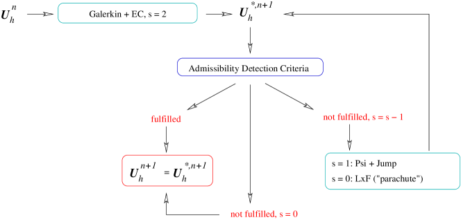
Figure 1: MOOD procedure with Galerkin and entropy correction, Psi+ jump stabilization and LxF-RD schemes

Before we start we require the following assumption on the numerical approximation $\rho^{h}(t),\mathbf{m}^{h}(t):=\rho^{h}(t)\mathbf{u}^{h}(t),E^{h}(t)\in V^{h}$ of $\rho(t),\mathbf{m}(t),E(t)$ obtained by our RD scheme (29).

Assumption 3.4.

We assume that there exist two positive constants $\underline{\rho}$ and $\overline{E}$ such that

$$\rho^{h}(t)\geq\underline{\rho}>0\qquad E^{h}(t)\leq\overline{E}\text{ uniformly for }h\to 0.$$ (30)

The physical meaning of this assumption is that no vacuum appears. The second assumption (30) implies then that the speed $|\mathbf{u}^{h}|$ is bounded since $|\mathbf{u}^{h}|^{2}\leq\frac{2E^{h}}{\rho^{h}}\leq\frac{2\overline{E}}{\underline{\rho}}<C.$ As it is described in [39, 22], Assumption 3.4 implies that the density is also bounded from above and the energy is bounded from below. Consequently, the pressure and temperature are bounded from above and below as well.

Conservation

The main feature of RD is the fact that it is interpreted in fluctuation splitting form which is related to the conservative form used in classical finite volume/finite difference schemes. All of the RD schemes are locally conservative as long as condition (12) holds. Since it is working locally, the conservation is also ensured even if the spatial discretization scheme differs between two neighboring elements which are essential important if the MOOD procedure is applied.

Actually, Assumption 3.3 is important to prove the Lax-Wendroff theorem [6]. We need this assumption as well inside our consistency analysis. One should see this assumption as asserting continuity of the residual components (or signals) $\Phi_{\sigma}^{K}$ with respect to the nodal values of $\mathbf{U}$; in particular, when $\mathbf{U}$ is constant, $\Phi_{\sigma}^{K}=0$. Note that the proof of the Lax-Wendroff theorem when $\Phi_{\sigma}^{K}$ satisfies Assumption 3.3 is still valid if the number of arguments in $\Phi_{\sigma}^{K}$ is bounded independently of $h$ and the element $K$. In practice, this is always true if the triangulation is uniform, since the arguments of $\Phi_{\sigma}^{K}$ are contained in some neighborhood of $\sigma$ comprising a finite number of points. Finally, we like to point out that using the entropy correction term does not affect those results due to its conservation property, i.e. $\sum\limits_{\sigma\in K}r_{\sigma}^{K}=0$.

High-order accuracy for smooth solutions

There exist plenty of papers in the literature focusing on the high-order accuracy properties of RD schemes for steady and unsteady flows, cf. [30, 1, 3] in case a smooth solution is approximated. Here, we want to point out that due to the analysis of [2, 44] the application of entropy correction terms does not affect this property if sufficiently accurate quadratures formulas are used. Roughly speaking, for a sufficiently smooth solution, we obtain an $h^{p+1}$ order accurate approximation both in space in time using RD together with the DeC approach [1].

Positivity Preservation

Not all of the residuals named in Example 3.2 can ensure to keep the density and pressure (internal energy) positive for the Euler equations (1). However, at least in our parachute scheme, the LxF residual (19) should provide this property. In Appendix 8, we demonstrate that this is true under a certain CFL condition for both the time explicit and implicit RD schemes.

Detection Procedure

The detection procedure is essential and besides the positivity of density, other points are checked. We base our detections on physical/modelling and numerical considerations. The algorithm procedure is the following from [7]:

• Physical Admissibility Detection: The density and pressure at every degree of freedom have to remain positive.

• Computational Admissibility Detection: The numerical solution can not be undefined (Not-A-Number or Infinity).

• Plateau Detection: If we are on a plateau, we make sure that we do not break that area.

• Numerical Admissibility Detection: The solution is tested against oscillatory behaviour. Here, we test for a relaxed discrete maximum principle. If the criteria are activated, we test for smoothness meaning that we have natural oscillations inside the calculations.

Using the MOOD procedure, we can start with any RD scheme and fall back, in the worst case scenario, to the parachute scheme. Here, the parachute scheme is the local Lax-Friedrich (or Rusanov distributions). Its properties (positivity, entropy dissipation) are recalled in the Appendix 8. Due to the finite number of cells and loops, the procedure converges. In the following part, we use the MOOD procedure to ensure the positivity of density and pressure at every degree of freedom.

4 Consistency Analysis

We investigate the consistency of our semi-discrete RD scheme (29). We will show that for the numerical solution $\mathbf{U}^{h}=(\rho^{h},\mathbf{m}^{h},E^{h})$ calculated by semi-discrete RD

$$\left[\int_{\Omega}\mathbf{U}^{h}\cdot\varphi{\mathrm{d}{\mathbf{x}}}\right]_{t=0}^{t=\tau}=\int_{0}^{\tau}\int_{\Omega}\partial_{t}\varphi\cdot\mathbf{U}^{h}+{\mathbf{f}}(\mathbf{U}^{h}):\nabla_{\mathbf{x}}\varphi{\mathrm{d}{\mathbf{x}}}{\mathrm{d}{t}}+\int_{0}^{\tau}\mathbf{e}^{h}(t,\varphi){\mathrm{d}{t}}$$ (31)

holds for all $\varphi\in C^{p+1}([0,T]\otimes\overline{\Omega},\mathbb{R}^{2+d})$ where the error $\mathbf{e}^{h}\to 0$ if $h\to 0$. Next, we specify $\mathbf{e}^{h}$ and demonstrate how we can ensure (31). Note that the consistency of the total energy, cf. Definition 2.1 (energy inequality), follows from the global conservation property of the scheme. Therefore, we restrict ourself in the following investigation on the density $\rho$ and momentum $\mathbf{m}$. However, to demonstrate the consistency estimation, we need a weak BV estimate where we focus on the entropy behavior. Therefore, we will describe as well the error of the entropy inequality. We derive finally the consistency formulation for $\mathcal{U}^{h}=(\rho^{h},\mathbf{m}^{h},\eta^{h})$. First, we realize that for all $\varphi\in C^{p+1}([0,T]\times\overline{\Omega},\mathbb{R}^{2+d})$

$$\left[\int_{\Omega}\mathbf{U}^{h}\varphi{\mathrm{d}{\mathbf{x}}}\right]_{t=0}^{t=\tau}=\int_{0}^{\tau}\int_{\Omega}\frac{{\mathrm{d}{}}}{{\mathrm{d}{t}}}\left(\mathbf{U}^{h}\varphi\right){\mathrm{d}{\mathbf{x}}}{\mathrm{d}{t}}=\int_{0}^{\tau}\int_{\Omega}\mathbf{U}^{h}\partial_{t}\varphi+\varphi\partial_{t}\mathbf{U}^{h}{\mathrm{d}{\mathbf{x}}}{\mathrm{d}{t}}$$ (32)

and for the last term, we have to apply the RD scheme in the semi-discrete setting (29) for $\partial_{t}\mathbf{U}^{h}$ and derive the error which we have to estimate.

4.1 Consistency Errors

The consistency analysis is independent of the choice of the residual. The only thing that matter, is that for the whole series of schemes used in the MOOD procedure, each scheme has the same total residual on each element: this guaranties local conservation. The choice of the residual will play a role in the entropy dissipation structure, cf. Section 4.2.

For any $\varphi\in C^{p+1}([0,T]\times\overline{\Omega},\mathbb{R}^{2+d})$, $\Pi_{h}\varphi$ will be

$$\Pi_{h}\varphi=\sum\limits_{\sigma}\varphi_{\sigma}\phi_{\sigma}$$

its approximation in $V^{h}$, and $t\in[t_{n},t_{n+1}[$

$$\tilde{\varphi}=\sum\limits_{\sigma}\varphi_{\sigma}^{n}1_{C_{\sigma}}.$$

We can rewrite as

$$\left[\int_{\Omega}\mathbf{U}^{h}\varphi{\mathrm{d}{\mathbf{x}}}\right]_{t=0}^{t=\tau}=\left[\int_{\Omega}\mathbf{U}^{h}\big{(}\varphi-\tilde{\varphi}\big{)}{\mathrm{d}{\mathbf{x}}}\right]_{t=0}^{t=\tau}+\left[\int_{\Omega}\mathbf{U}^{h}\tilde{\varphi}{\mathrm{d}{\mathbf{x}}}\right]_{t=0}^{t=\tau},$$

and, since $|C_{\sigma}|=\int_{\Omega}\phi_{\sigma}$, under $h=O(\Delta t)$, we get

$$\left|\left[\int_{\Omega}\mathbf{U}^{h}\big{(}\varphi-\tilde{\varphi}\big{)}{\mathrm{d}{\mathbf{x}}}\right]_{t=0}^{t=\tau}\right|\leq Ch\max_{t\in[0,\tau]}\|\mathbf{U}^{h}\|_{L^{1}}.$$

Then, we write

$$\left[\int_{\Omega}\mathbf{U}^{h}\tilde{\varphi}{\mathrm{d}{\mathbf{x}}}\right]_{t=0}^{t=\tau}=\int_{\Omega}\tilde{\varphi}_{t}\cdot\mathbf{U}^{h}+\tilde{\varphi}\partial_{t}\mathbf{U}^{h}{\mathrm{d}{\mathbf{x}}}.$$

We have

$$\begin{split}\int_{\Omega}\tilde{\varphi}\partial_{t}\mathbf{U}^{h}{\mathrm{d}{\mathbf{x}}}&=\sum\limits_{\sigma}|C_{\sigma}|\tilde{\varphi}_{\sigma}\partial_{t}\big{(}\mathbf{U}^{h}_{\sigma}\big{)}=-\sum_{K}\sum\limits_{\sigma\in K}\tilde{\varphi}_{\sigma}\Phi_{\sigma}^{K}(\mathbf{U}^{h})\\ &=-\sum_{K}\sum\limits_{\sigma\in K}\tilde{\varphi}_{\sigma}\bigg{(}-\int_{K}\nabla\phi_{\sigma}{\mathbf{f}}(\mathbf{U}^{h}){\mathrm{d}{\mathbf{x}}}+\int_{\partial K}\phi_{\sigma}\mathbf{f}^{\mathrm{num}}(\mathbf{U}^{h,K},\mathbf{U}^{h,K^{+}}){\mathrm{d}{\gamma}}\\ &\qquad+\sum_{K}\sum_{\sigma\in K}\tilde{\varphi}_{\sigma}\big{(}\Phi_{\sigma}^{K}(\mathbf{U}^{h})-\Phi_{\sigma}^{K,Gal}(\mathbf{U}^{h})\big{)},\end{split}$$

where we have set

$$\Phi_{\sigma}^{K,Gal}(\mathbf{U}^{h})=-\int_{K}\nabla\phi_{\sigma}{\mathbf{f}}(\mathbf{U}^{h}){\mathrm{d}{\mathbf{x}}}+\int_{\partial K}\phi_{\sigma}\mathbf{f}^{\mathrm{num}}(\mathbf{U}^{h,K},\mathbf{U}^{h,K^{+}}){\mathrm{d}{\gamma}}.$$

Since $\sum_{\sigma\in K}\Phi_{\sigma}^{K}(\mathbf{U}^{h})=\sum_{\sigma\in K}\Phi_{\sigma}^{K,Gal}(\mathbf{U}^{h})$, and using the conditions at the boundary (periodic or no-flux boundary), we can rewrite this as

$$\begin{split}\int_{\Omega}\tilde{\varphi}\partial_{t}\mathbf{U}^{h}{\mathrm{d}{\mathbf{x}}}&=-\int_{\Omega}\nabla\Pi_{h}\varphi\cdot{\mathbf{f}}(\mathbf{U}^{h}){\mathrm{d}{\mathbf{x}}}+\sum_{K}\sum_{\sigma,\sigma^{\prime}\in K}\big{(}\varphi_{\sigma}-\varphi_{\sigma^{\prime}}\big{)}\big{(}\Phi_{\sigma}^{K}(\mathbf{U}^{h})-\Phi_{\sigma}^{K,Gal}(\mathbf{U}^{h})\big{)}.\end{split}$$

Collecting all the pieces together, we get (31) with

$$\mathbf{e}^{h}(t,\varphi)=\underbrace{\sum_{K}\sum_{\sigma,\sigma^{\prime}\in K}\big{(}\varphi_{\sigma}-\varphi_{\sigma^{\prime}}\big{)}\big{(}\Phi_{\sigma}(\mathbf{U}^{h})-\Phi_{\sigma}^{K,Gal}(\mathbf{U}^{h})\big{)}}_{(I)}+\underbrace{\bigg{[}\int_{\Omega}\mathbf{U}^{h}\big{(}\varphi-\tilde{\varphi}\big{)}{\mathrm{d}{\mathbf{x}}}\bigg{]}_{t=0}^{t=\tau}}_{(II)}+\underbrace{\int_{\Omega}\big{(}\Pi_{h}\varphi-\varphi\big{)}:{\mathbf{f}}(\mathbf{U}^{h}){\mathrm{d}{\mathbf{x}}}}_{(III)}.$$ (33)

We have already seen that for a bounded sequence $\mathbf{U}^{h}$ the terms $(II)$ and $(III)$ will converge to $0$, so the only thing to study is the behavior of the term $(I)$. Term $(I)$ will be discussed in the following part where we demonstrate that this term tends to zero. Therefore, we need a weak BV estimation derived from the entropy inequality.

4.2 Weak BV estimates for entropy dissipative RD schemes

For the consistency estimation of the entropy inequality and to estimate term $(I)$, we need additionally to demonstrate the weak BV estimation for our RD scheme (29). Before, we note that Assumption 3.4 is related to the mathematical entropy function (2) as demonstrated in [39, Lemma 3.1 and B2], it is equivalent to the strict convexity of the mathematical entropy function (2), i.e.

$$\exists\underline{\eta}_{0}>0:\frac{{\mathrm{d}{}}^{2}\eta(\mathbf{U}^{h})}{{\mathrm{d}{\mathbf{U}}}^{2}}\geq\underline{\eta}_{0}\mathcal{I}$$ (34)

where $\mathcal{I}$ is a unity matrix.

Now, we start with our semi-discrete entropy RD scheme (26). We recall its construction. Starting for a family of residuals $\Phi_{\sigma}^{K}(\mathbf{U}^{h})$ that satisfies the conservation relations

$$\sum\limits_{\sigma\in K}\Phi_{\sigma}^{K}(\mathcal{U}^{h})=\int_{\partial K}\mathbf{f}^{\mathrm{num}}(\mathbf{U}^{h,K},\mathbf{U}^{h,K^{+}},{\mathbf{n}}){\mathrm{d}{\gamma}}.$$

By introducing a correction of the form $\alpha_{K}\big{(}\mathbf{V}_{\sigma}-\overline{\mathbf{V}}_{K}\big{)}$, we can choose $\alpha_{K}$ such that $\Psi_{\sigma}^{K}(\mathbf{U}^{h})=\Phi_{\sigma}^{K}(\mathbf{U}^{h})+\alpha_{K}\big{(}\mathbf{V}_{\sigma}-\overline{\mathbf{V}}_{K}\big{)}$ satisfies in each element

$$\sum\limits_{\sigma\in K}\Psi_{\sigma}^{K}(\mathbf{U}^{h})=\int_{\partial K}\mathbf{f}^{\mathrm{num}}(\mathbf{U}^{h,K},\mathbf{U}^{h,K^{+}},{\mathbf{n}}){\mathrm{d}{\gamma}},$$

and

$$\sum\limits_{\sigma\in K}\langle\mathbf{V}_{\sigma},\Psi_{\sigma}^{K}(\mathbf{U}^{h})\rangle=\int_{\partial K}\mathbf{g}^{\mathrm{num}}(\mathbf{U}^{h,K},\mathbf{U}^{h,K^{+}},{\mathbf{n}}){\mathrm{d}{\gamma}},$$

where the numerical flux $\mathbf{g}^{\mathrm{num}}$ is consistent with the entropy flux $\mathbf{g}$. Then we modify again the residuals and define

$$\Theta_{\sigma}^{K}(\mathbf{U})=\Psi_{\sigma}^{K}+\lambda h_{K}^{\zeta}\int_{\partial K}\raisebox{-2.5pt}{\leavevmode\resizebox{0.0pt}{8.3333pt}{\raisebox{2.5pt}{$[\mkern-3.0mu[$}}}\nabla\phi_{\sigma}\raisebox{-2.5pt}{\leavevmode\resizebox{0.0pt}{8.3333pt}{\raisebox{2.5pt}{$]\mkern-3.0mu]$}}}\cdot\raisebox{-2.5pt}{\leavevmode\resizebox{0.0pt}{10.53328pt}{\raisebox{2.5pt}{$[\mkern-3.0mu[$}}}\nabla\mathbf{V}^{h}\raisebox{-2.5pt}{\leavevmode\resizebox{0.0pt}{10.53328pt}{\raisebox{2.5pt}{$]\mkern-3.0mu]$}}}{\mathrm{d}{\gamma}}$$ (35)

with $\zeta\geq 2$. Here, $\lambda>0$ depends on the maximum of the eigenvalues of the Jacobian matrices. This residual still satisfies the conservation requirement and we have

$$\sum\limits_{\sigma\in K}\langle\mathbf{V}_{\sigma},\Theta_{\sigma}^{K}(\mathbf{U}^{h})\rangle=\int_{\partial K}\mathbf{g}^{\mathrm{num}}(\mathbf{U}^{h,K},\mathbf{U}^{h,K^{+}},{\mathbf{n}}){\mathrm{d}{\gamma}}+\lambda h_{K}^{\zeta}\int_{\partial K}\left\lVert\raisebox{-2.5pt}{\leavevmode\resizebox{0.0pt}{10.53328pt}{\raisebox{2.5pt}{$[\mkern-3.0mu[$}}}\nabla\mathbf{V}^{h}\raisebox{-2.5pt}{\leavevmode\resizebox{0.0pt}{10.53328pt}{\raisebox{2.5pt}{$]\mkern-3.0mu]$}}}\right\rVert^{2}{\mathrm{d}{\gamma}},$$

where $\left\lVert\cdot\right\rVert$ denotes the Euclidian norm in the following. In the case of the parachute scheme, the entropy production is built in into the residual, and we have a similar formula with $\zeta=2$, this is why $\zeta=2$ is the factor of choice.

Using this, and proceeding as before, for any positive test function $\varphi\in C^{p+1}([0,T]\times\overline{\Omega},\mathbb{R})$, we get

$$\left[\int_{\Omega}\eta^{h}\varphi{\mathrm{d}{\mathbf{x}}}\right]_{t=0}^{t=\tau}=\int_{0}^{\tau}\int_{\Omega}\partial_{t}\varphi\cdot\eta^{h}+\mathbf{g}(\mathbf{U}^{h}):\nabla_{\mathbf{x}}\varphi{\mathrm{d}{\mathbf{x}}}{\mathrm{d}{t}}+\int_{0}^{\tau}\mathbf{e_{\eta}}^{h}(t,\varphi){\mathrm{d}{t}}.$$ (36)

Setting $\Xi^{K}_{\sigma}(\mathbf{U}^{h})=\langle\mathbf{V}_{\sigma},\Theta^{K}_{\sigma}(\mathbf{U}^{h})\rangle$ and $\Xi_{\sigma}^{K,Gal}=\langle\mathbf{V}_{\sigma},\Theta^{K,Gal}_{\sigma}(\mathbf{U}^{h})\rangle$ to simplify the notations, we have

$$\begin{split}\mathbf{e_{\eta}}^{h}(t,\varphi)&=\underbrace{\sum_{K}\sum_{\sigma,\sigma^{\prime}\in K}\big{(}\varphi_{\sigma}-\varphi_{\sigma^{\prime}}\big{)}\big{(}\Xi_{\sigma}(\mathbf{U}^{h})-\Xi_{\sigma}^{K,Gal}(\mathbf{U}^{h})\big{)}}_{(I)}+\underbrace{\bigg{[}\int_{\Omega}\mathbf{V}^{h}\big{(}\varphi-\tilde{\varphi}\big{)}{\mathrm{d}{\mathbf{x}}}\bigg{]}_{t=0}^{t=\tau}}_{(II)}+\underbrace{\int_{\Omega}\big{(}\Pi_{h}\varphi-\varphi\big{)}:\mathbf{g}(\mathbf{U}^{h}){\mathrm{d}{\mathbf{x}}}}_{(III)}\\ &+\underbrace{\sum\limits_{K}\lambda h_{K}^{\zeta}\int_{\partial K}\left\lVert\raisebox{-2.5pt}{\leavevmode\resizebox{0.0pt}{10.53328pt}{\raisebox{2.5pt}{$[\mkern-3.0mu[$}}}\nabla\mathbf{V}^{h}\raisebox{-2.5pt}{\leavevmode\resizebox{0.0pt}{10.53328pt}{\raisebox{2.5pt}{$]\mkern-3.0mu]$}}}\right\rVert^{2}{\mathrm{d}{\gamma}}}_{(IV)}.\end{split}$$ (37)

In particular, taking $\varphi=1$, we obtain

$$\left[\int_{\Omega}\eta^{h}{\mathrm{d}{\mathbf{x}}}\right]_{t=0}^{t=\tau}+\sum\limits_{e\in\mathcal{E}}\lambda h_{K}^{\zeta}\int_{e}\left\lVert\raisebox{-2.5pt}{\leavevmode\resizebox{0.0pt}{10.53328pt}{\raisebox{2.5pt}{$[\mkern-3.0mu[$}}}\nabla\mathbf{V}^{h}\raisebox{-2.5pt}{\leavevmode\resizebox{0.0pt}{10.53328pt}{\raisebox{2.5pt}{$]\mkern-3.0mu]$}}}\right\rVert^{2}{\mathrm{d}{\gamma}}=0$$ (38)

Let us define

$$\left\lVert\|\mathbf{U}^{h}\|\right\rVert^{2}:=\sum\limits_{e\in\mathcal{E}}h_{K}^{\zeta}d\int_{e}\left\lVert\raisebox{-2.5pt}{\leavevmode\resizebox{0.0pt}{10.53328pt}{\raisebox{2.5pt}{$[\mkern-3.0mu[$}}}\nabla\mathbf{V}^{h}\raisebox{-2.5pt}{\leavevmode\resizebox{0.0pt}{10.53328pt}{\raisebox{2.5pt}{$]\mkern-3.0mu]$}}}\right\rVert^{2}{\mathrm{d}{\gamma}}.$$

This is a norm: If $\left\lVert\|\mathbf{U}^{h}\|\right\rVert=0$, this means that across any edge, $\raisebox{-2.5pt}{\leavevmode\resizebox{0.0pt}{10.53328pt}{\raisebox{2.5pt}{$[\mkern-3.0mu[$}}}\nabla\mathbf{V}^{h}\raisebox{-2.5pt}{\leavevmode\resizebox{0.0pt}{10.53328pt}{\raisebox{2.5pt}{$]\mkern-3.0mu]$}}}=0$, i.e. $\mathbf{V}^{h}$ is a given polynomial over $\mathbb{R}^{d}$, and because it is compactly supported, $\mathbf{U}^{h}=0$. We will have under the assumptions of boundedness from above and below (for the density) that

$$\|\|\mathbf{U}^{h}\|\|\leq C(\mathbf{U}^{h}(0))\leq C^{\prime}\int_{\Omega}|\mathbf{V}(\mathbf{x},0)|{\mathrm{d}{\mathbf{x}}}.$$

We have, for any $C$ and $C^{\prime}$,

$$\int_{e}\left\lVert\raisebox{-2.5pt}{\leavevmode\resizebox{0.0pt}{10.53328pt}{\raisebox{2.5pt}{$[\mkern-3.0mu[$}}}\mathbf{V}^{h}\raisebox{-2.5pt}{\leavevmode\resizebox{0.0pt}{10.53328pt}{\raisebox{2.5pt}{$]\mkern-3.0mu]$}}}\right\rVert^{2}{\mathrm{d}{\gamma}}=\int_{e}\|\nabla(\mathbf{V}^{h}-C)_{|K}-\nabla(\mathbf{V}^{h}-C^{\prime})_{|K^{\prime}}\|^{2}.$$

Since the number of degrees of freedom in $K$ and $K^{\prime}$ is bounded, and because the mesh is regular, there exists $\alpha$ and $\beta$ independent of $K$ and $K^{\prime}$ such that

$$\alpha h_{K}^{d+\zeta-3}\sum\limits_{\sigma,\sigma^{\prime}\in K\mathbf{U}\cup K^{\prime}}\left\lVert\mathbf{V}_{\sigma}-\mathbf{V}_{\sigma^{\prime}}\right\rVert^{2}\leq h_{K}^{\zeta}\int_{e}\left\lVert\raisebox{-2.5pt}{\leavevmode\resizebox{0.0pt}{10.53328pt}{\raisebox{2.5pt}{$[\mkern-3.0mu[$}}}\nabla\mathbf{V}^{h}\raisebox{-2.5pt}{\leavevmode\resizebox{0.0pt}{10.53328pt}{\raisebox{2.5pt}{$]\mkern-3.0mu]$}}}\right\rVert^{2}{\mathrm{d}{\gamma}}\leq\beta h_{K}^{d+\zeta-3}\sum\limits_{\sigma,\sigma^{\prime}\in K\cup K^{\prime}}\|\mathbf{V}_{\sigma}-\mathbf{V}_{\sigma^{\prime}}\|^{2}.$$ (39)

Note that $d+\zeta-3\geq d-1$. In the end, the norm $\left\lVert\|~{}.~{}\|\right\rVert$ and

$$\sum_{K}\sum_{\sigma\in K}h_{K}^{\frac{d+\zeta-3}{2}}\sum_{\sigma_{1},\sigma_{2}\in\mathcal{S}_{\sigma}}\|\mathbf{U}_{\sigma_{1}}-\mathbf{U}_{\sigma_{2}}\|$$

are equivalent, because for $\sigma\in K$, $\mathcal{S}_{\sigma}$ is contained in the set of DOFs in $K$, and those of the neighbouring elements to $K$. We recall that $\lambda$ depends on the maximum of $\mathbf{U}^{h}$ over the mesh which is bounded. We point out that (38) together with (39) yields the BV estimate, namely

$$\sum_{K}\sum_{\sigma\in K}h_{K}^{\frac{d+\zeta-3}{2}}\sum_{\sigma_{1},\sigma_{2}\in\mathcal{S}_{\sigma}}\|\mathbf{U}_{\sigma_{1}}-\mathbf{U}_{\sigma_{2}}\|\leq C.$$

Combining (39) with the Assumption 3.3 on the residuals, the relation (33) and in particular its term $(I)$, since $|\varphi_{\sigma}-\varphi_{\sigma^{\prime}}|\leq C\|\nabla\varphi\|_{\infty}h$, we see that

$$\|\mathbf{e}_{\eta}^{h}(t,\varphi)\|\leq Ch^{d-1+1-\frac{d+\zeta-3}{2}}=Ch^{d-\frac{d+\zeta-3}{2}}\rightarrow 0$$

when $h\rightarrow 0$, as soon as $\zeta\geq 2$. Here $(I)$ corresponds to the first term in (33) as well as in (37). The constant $C$ only depends on the $L^{\infty}$ bound on the numerical solution, cf. Assumption 3.4, where the constant $C$ from Assumption 3.3 depends only on the geometrical regularity of the mesh.

In total, we have shown the following results:

Theorem 4.1 (Consistency Formulation).

Let $\mathbf{U}^{h}$ be a solution of the RD scheme with the MOOD approach on the interval $[0,T]$ with the initial data $\mathbf{U}^{h}_{0}$. Under our assumptions 3.1, 3.3, and 3.4 we have the following results for all $\tau\in(0,T]$:

• for all $\varphi\in C^{p+1}([0,T]\times\overline{\Omega})$:

  $$\left[\int_{\Omega}\rho^{h}\varphi{\mathrm{d}{\mathbf{x}}}\right]_{t=0}^{t=\tau}=\int_{0}^{\tau}\int_{\Omega}\rho_{h}\partial_{t}\varphi+\mathbf{m}^{h}\cdot\nabla_{\mathbf{x}}\varphi{\mathrm{d}{\mathbf{x}}}{\mathrm{d}{t}}+\int_{0}^{\tau}e_{\rho^{h}}(t,\varphi){\mathrm{d}{t}};$$ (40)

• for all $\varphi\in C^{p+1}([0,T]\times\overline{\Omega};\mathbb{R}^{d})$:

  $$\left[\int_{\Omega}\mathbf{m}^{h}\mathbf{\varphi}{\mathrm{d}{\mathbf{x}}}\right]_{t=0}^{t=\tau}=\int_{0}^{\tau}\int_{\Omega}\mathbf{m}^{h}\partial_{t}\mathbf{\varphi}+\frac{\mathbf{m}^{h}\otimes\mathbf{m}^{h}}{\rho^{h}}:\nabla_{\mathbf{x}}\mathbf{\varphi}+p^{h}\operatorname{div}_{\mathbf{x}}\mathbf{\varphi}{\mathrm{d}{\mathbf{x}}}{\mathrm{d}{t}}+\int_{0}^{\tau}e_{\mathbf{m}^{h}}(t,\mathbf{\varphi}){\mathrm{d}{t}};$$ (41)

• for all $\varphi\in C^{p+1}([0,T]\times\overline{\Omega}),\;\varphi\geq 0$:

  $$\left[\int_{\Omega}\eta^{h}\varphi{\mathrm{d}{\mathbf{x}}}\right]_{t=0}^{t=\tau}\leq\int_{0}^{\tau}\int_{\Omega}\eta^{h}\partial_{t}\varphi+(\eta^{h}\mathbf{u}^{h})\cdot\nabla_{\mathbf{x}}\mathbf{\varphi}{\mathrm{d}{\mathbf{x}}}{\mathrm{d}{t}}+\int_{0}^{\tau}e_{\eta^{h}}(t,\varphi){\mathrm{d}{t}};$$ (42)

• $\int_{\Omega}E^{h}(\tau){\mathrm{d}{\mathbf{x}}}=\int_{\Omega}E^{h}_{0}{\mathrm{d}{\mathbf{x}}}$

• The errors $e_{j^{h}}$, $(j=\rho,\mathbf{m},\eta)$ tend to zero under mesh refinement

  $$\left\lVert e_{j^{h}}\right\rVert_{L^{1}(0,T)}\to 0\text{ if }h\to 0.$$ (43)

Remark 4.2 (MOOD and LxF-Residual).

Due to our assumptions, we have proven that all of our considered schemes are consistent. However, it is known that some of those schemes will have stability issues and violate the positivity of pressure and density inside our numerical simulations. To overcome this issue, we use the MOOD approach locally. As our parachute scheme, we apply the LxF residual which has the highest amount of dissipation and acts around the shock analogously to the local Lax-Friedrich schemes where convergence for dissipative weak solutions has been proven in [22] also for the fully-discrete case.

5 Convergence to dissipative weak solutions

We have demonstrated that the RD methods yield a consistent approximation for the Euler equations (1) Theorem 4.1. Due to the MOOD approach we can also ensure that the underlying physical laws, e.g. positivity of density and pressure, are fulfilled. At all, we demonstrated that our final implemented scheme is high-order, structure preserving and consistent. These are exactly the properties which are needed to prove a convergence result in the spirit of [22, 39, 38]. We start with the weak convergence theorem similar to [38].

Theorem 5.1 (Weak convergence).

Let $\mathcal{U}^{h}=\{\rho^{h},\mathbf{m}^{h},\eta^{h}\}_{h\to 0}$ be a family of numerical solutions generated by the RD schemes (29) with the MOOD. Let Assumptions 3.1, 3.4, and 3.3 hold. Then there exists a subsequence $\mathcal{U}^{h}$ (denoted again by $\mathcal{U}^{h}$) such that

$$\rho^{h} \to\rho\text{ weakly-(*) in }L^{\infty}((0,T)\times\Omega)$$ (44)

$$\eta^{h} \to\eta\text{ weakly-(*) in }L^{\infty}((0,T)\times\Omega)$$

$$\mathbf{m}^{h} \to\mathbf{m}\text{ weakly-(*) in }L^{\infty}((0,T)\times\Omega;\mathbb{R}^{2}))$$

as $h\to 0$ and $(\rho,\mathbf{m},\eta)$ is a DW solution of the complete Euler system (1).

Proof.

The proof follows analogous steps as presented in [23, 38]. It uses the fact that the RD schemes with the MOOD approach lead to consistent and stable approximation of the Euler equations. ∎

In numerical simulations weak convergence is not really suitable for visualization of a DW solution. It is more convenient to work with the Cesaro averages, known as $\mathcal{K}$-convergence in such context. As demonstrated in [23, Theorem 10.5], we obtain strong convergence of the Cesaro averages to a DW solution as well as strong convergence of the approximate deviation of the associated Young measures. Here, we mean with strong convergence of Cesaro averages $\mathcal{U}^{h_{n}}=(\rho^{h_{n}},\mathbf{m}^{h_{n}},\eta^{h_{n}})$ that

$$\frac{1}{N}\sum_{n=1}^{N}\mathcal{U}^{h_{n}}\to\mathcal{U}\text{ as }N\to\infty\text{ in }L^{q}((0,T)\times\Omega,\mathbb{R}^{4})\text{ for any }1\leq q<\infty.$$

In addition, if we have more informations on the regularity of the solutions, we get the strong convergence of the sequence of approximated solutions by adapting the proof [23, Theorem 10.6] to our RD setting.

Theorem 5.2 (Strong Convergence of the RD scheme).

Let $\mathcal{U}^{h}=\{\rho^{h},\mathbf{m}^{h},\eta^{h}\}_{h\to 0}$ be numerical solutions of RD scheme (29) with the MOOD approach. Let the initial data be $\rho^{h}_{0},\mathbf{m}_{0}^{h}$ and $\eta_{0}^{h},\rho_{0}\geq\underline{\rho}>0,(1-\gamma)\eta_{0}\geq\underline{\rho s}$. Further, let Assumptions 3.1, 3.4, and 3.3 hold. Then, the following holds:

• weak solution:
  If $\mathcal{U}=[\rho,\mathbf{m},\eta]$ obtained as a weak^∗limit of $\{\rho^{h},\mathbf{m}^{h},\eta^{h}\}_{h\to 0}$, is a weak entropy solution and emanating from the initial data $\mathcal{U}_{0}$, then $\nu_{t,\mathbf{x}}=\delta_{\mathcal{U}(t,\mathbf{x})}$ for a.a. $(t,\mathbf{x})\in(0,T)\times\Omega$, and

  $$(\rho^{h},\mathbf{m}^{h},\eta^{h}) \to(\rho,\mathbf{m},\eta)\text{ in }L^{q}((0,T)\times\Omega;\mathbb{R}^{4}),$$

  $$E(\mathcal{U}^{h})=\frac{1}{2}\frac{|\mathbf{m}^{h}|^{2}}{\rho^{h}}+\rho^{h}e(\rho^{h},\eta^{h}) \to\frac{1}{2}\frac{|\mathbf{m}|^{2}}{\rho}+\rho e(\rho,\eta)\text{ in }L^{q}((0,T)\times\Omega)$$

  for any $1\leq q<\infty$

• strong solution:
  Suppose that the Euler system admits a strong solution $\mathcal{U}$ in the class $\rho,\eta\in W^{1,\infty}((0,T)\times\Omega),\mathbf{m}\in W^{1,\infty}((0,T)\times\Omega;\mathbb{R}^{2})$, $\rho\geq\underline{\rho}>0$ in $[0,T]\times\Omega$ emanating from the initial data $\mathcal{U}_{0}$. Then, for any $1\leq q<\infty$ and $h\to 0$

  $$(\rho^{h},\mathbf{m}^{h},\eta^{h}) \to(\rho,\mathbf{m},\eta)\text{ in }L^{q}((0,T)\times\Omega;\mathbb{R}^{4}),$$

  $$E(\mathcal{U}^{h}) \to E(\mathcal{U})\text{ in }L^{q}((0,T)\times\Omega).$$

• classical solutions:
  Let $\Omega\in\mathbb{R}^{d}$ be a bounded Lipschitz domain and $\rho\in C^{1}([0,T]\times\overline{\Omega})$, $\rho\geq\overline{\rho}>0,\;\mathbf{m}\in C^{1}([0,T]\times\overline{\Omega};\mathbb{R}^{2}),\;\eta\in C^{1}([0,T]\times\overline{\Omega})$. Then $\mathcal{U}=(\rho,\mathbf{m},\eta)$ is a classical solution to the Euler system and

  $$(\rho^{h},\mathbf{m}^{h},\eta^{h}) \to(\rho,\mathbf{m},\eta)\text{ in }L^{q}((0,T)\times\Omega,\mathbb{R}^{4})$$

  as $h\to 0$, for any $q\geq 1$.

Proof.

Analog to [23, Theorem 10.6]. ∎

6 Numerical Experiments

In the following section, we verify Theorem 5.2 by a numerical experiment. We consider a moving vortex. Initially, an isentropic perturbation $(\delta S=0)$ is applied to the system, such that

$$\delta u =-\overline{y}\frac{\beta}{2\pi}e^{(1-r^{2})/2},$$

$$\delta v =\overline{x}\frac{\beta}{2\pi}e^{(1-r^{2})/2},$$

$$\delta T =-\frac{(\gamma-1)\beta^{2}}{8\gamma\pi^{2}}e^{(1-r^{2})/2}.$$

The initial conditions are thus set to

$$\rho =T^{1/(\gamma-1)}=(T_{\infty}+\delta T)^{1/(\gamma-1)}=\left[1-\frac{(\gamma-1)\beta^{2}}{8\gamma\pi^{2}}e^{(1-r^{2})/2}\right]^{1/(\gamma-1)},$$

$$\rho u =\rho(u_{\infty}+\delta u)=\rho\left[1-\overline{y}\frac{\beta}{2\pi}e^{(1-r^{2})/2}\right],$$

$$\rho v =\rho(v_{\infty}+\delta v)=\rho\left[1+\overline{x}\frac{\beta}{2\pi}e^{(1-r^{2})/2}\right],$$

$$\rho E =\frac{\rho^{\gamma}}{\gamma-1}+\frac{1}{2}\rho(u^{2}+v^{2}),$$

where $\beta=5,r=\overline{x}^{2}+\overline{y}^{2}$ and $(\overline{x},\overline{y})=((x-x_{0}),(y-y_{0}))$. The computational domain is a square with length $10$ and center $(0,0)$. Periodic boundary conditions are considered where we identify the left and right boundaries and the lower and upper boundaries with each other.

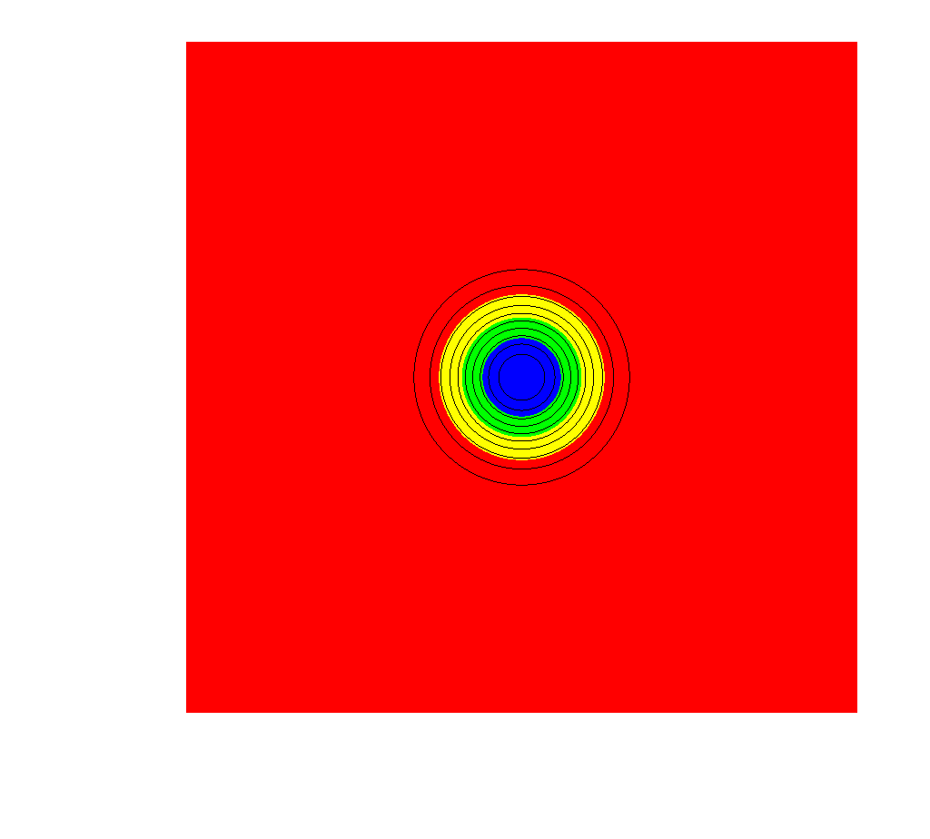
(a) Initial Condition

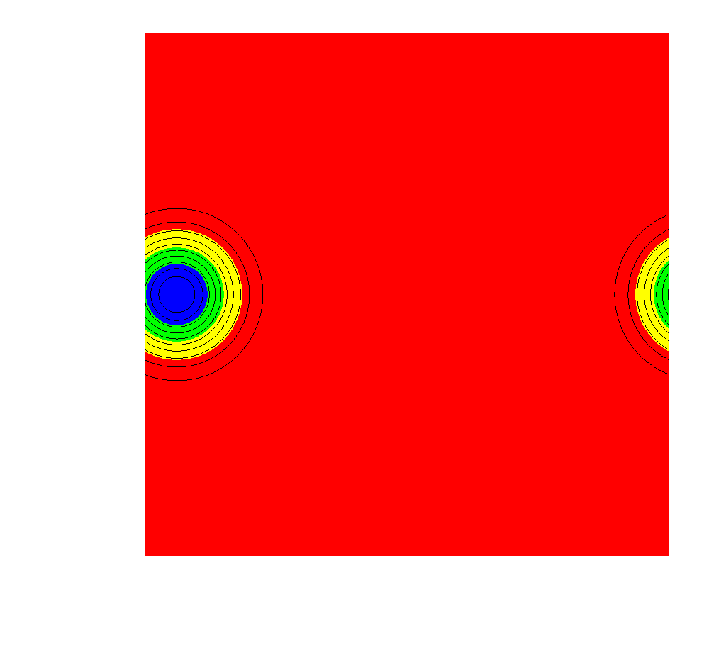
(b) Numerical Solution after 10000 steps

(c) Numerical Solution at T=10

Figure 2: Moving vortex at different time levels

The center of the vortex is set in $(0,0)$. The selected parameters of the unperturbed flow are set to $u_{\infty}=1$, $v_{\infty}=0$ for the velocities, $p_{\infty}=1$ for the density. In this first simulation, we apply the pure Galerkin residual with entropy correction and $B1$ polynomials on an unstructured trianglular mesh. The vortex is moving to the right and at $T=10$ we reach again our starting point as can be seen in Figure 2. The vortex is moving only to the right (it reduces to a simple advection), therefore, we have a classical smooth solution in this test case. From Theorem 5.2, a grid convergence investigation ensures that the errors decrease to the analytical solution. We verify this result in Figure (3), where we plot the error behaviors in respect to the number of elements and clearly a grid convergence can be recognized. For a more specific investigation of the order of various different RD schemes and more experiments, we refer again to [44, 40].

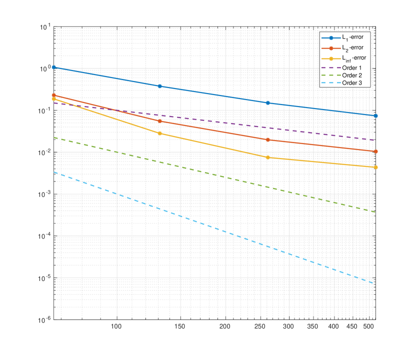
(a) Density $\rho$-error behavior

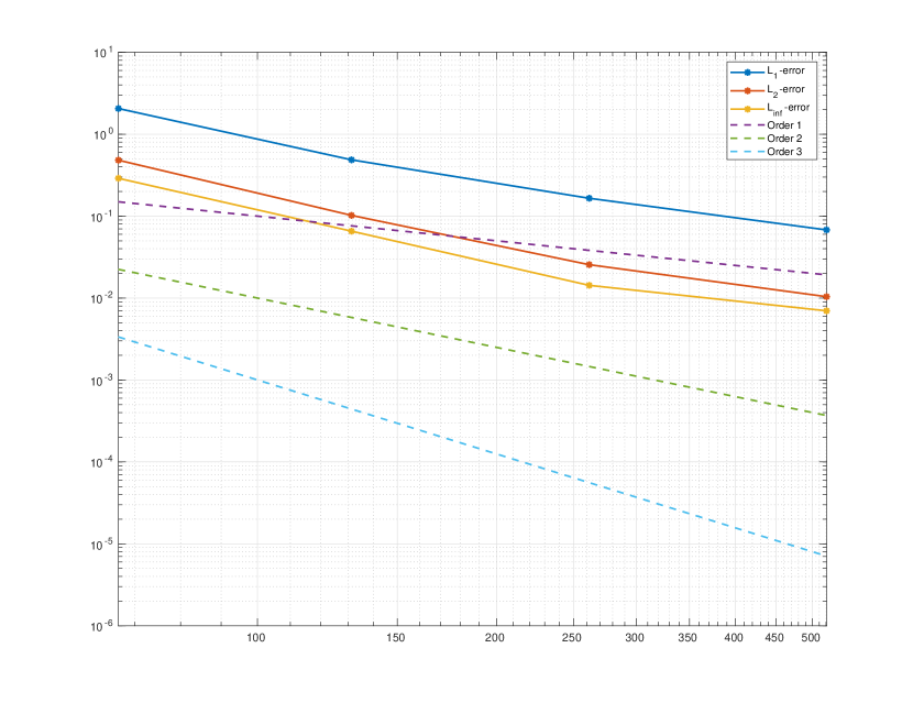
(b) Velocity $u$-error behavior

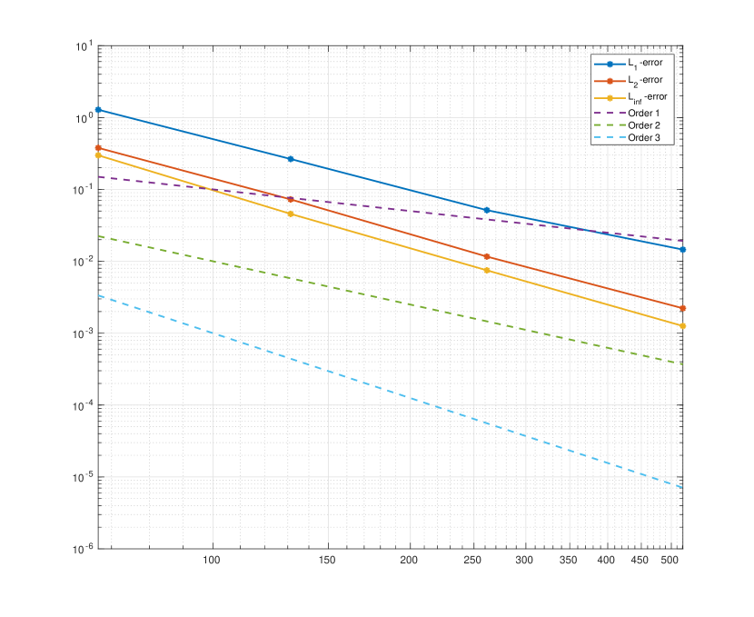
(c) Pressure $p$-error behavior

Figure 3: Error behaviour at $T=10$

7 Conclusion and Outlook

We have demonstrated a convergence analysis of the Euler equations via dissipative weak solutions for the general framework of residual distribution schemes including several high-order FE methods. Essential in our investigate was that the RD schemes ensure the underlying physical laws like positivity of internal energy and density and yields a consistent approximation of the Euler equations. We prove the consistency for every entropy dissipative RD schemes and so for all high-order finite element schemes which can be interpreted in this framework. The proof used a weak BV estimate which is derived by the entropy dissipative property of the considered RD scheme. Due to the results of [2, 5], we can guaranteed entropy dissipation of our considered RD scheme by the application of entropy correction terms as described in the mentioned literature. To guarantee the positivity of pressure and density, we have applied the MOOD approach and used as the parachute scheme the Lax-Friedrich residual which we have demonstrate that it is positivity preserving for both an explicit and and implicit time integration method. Our convergence analysis was restricted to the semi-discrete setting in the future, we plan to extend our investigations to the fully discrete framework [4, 25]. A unifying analysis for several high-order FE methods will also be considered. Similar convergence results can be expected for other structure-preserving schemes, see [33, 34, 27]. The concept of dissipative weak solutions is not restricted to the Euler equations, but it has been also used for the compressible Navier-Stokes equations [23, 42, 35], viscous magentohydrodynamics (MHD) [37] and viscous multi-component flows [36, 32]. However, no analytical and numerical results exists -up to our knowledge- focussing on non-viscous MHD or non-viscous multi-component/phase flows. Extensions of DW to those models will be considered in the future. In particular, the interpretation in multi-component seems very promising. Here, already in the description of the equations some of the quantities can be expressed in terms of measures and so the concept of dissipative measure-valued/weak solutions seems even more beneficial.

8 Appendix

Positivity property of the LxF residuals.

Explicit case

In the following part, we repeat the proof about the positivity of the local Lax-Friedrich (LxF) (or Rusanov) residual following [7]. For the time-integration, we apply a simple Euler step first. Independent of the interpretation of the degrees of freedom, we obtain:

$$\mathbf{U}_{\sigma}^{n+1}=\mathbf{U}_{\sigma}^{n}-\dfrac{\Delta t}{|C_{\sigma}|}\sum_{K|\sigma\in K}\Phi_{\sigma,\mathbf{x}}^{K,LxF}(\mathbf{U}^{n}).$$ (45)

For later, we can re-interpret $\mathbf{U}_{\sigma}^{n+1}$ using $|K_{\sigma}|=\dfrac{|K|}{N_{K}}$:

$$\mathbf{U}_{\sigma}^{n+1}=\sum_{K,\sigma\in K}\dfrac{|K_{\sigma}|}{|C_{\sigma}|}\mathbf{U}_{\sigma}^{K,\star}\text{ with }\mathbf{U}_{\sigma}^{K,\star}=\mathbf{U}_{\sigma}^{n}-\dfrac{\Delta t}{|K_{\sigma}|}\Phi_{\sigma,\mathbf{x}}^{K,LxF}(\mathbf{U}^{n}).$$ (46)

The LxF described in (19) can be interpreted in the following two ways:

1. The first version similar to the variational form $\Phi_{\sigma,\mathbf{x}}^{K,LxF}(\mathbf{U}^{h})=\int_{K}\phi_{\sigma}\text{ div }{\mathbf{f}}^{h}(\mathbf{U}^{h})\;d\mathbf{x}+\alpha_{K}\big{(}\mathbf{U}_{\sigma}-\overline{\mathbf{U}}\big{)}$, with ${\mathbf{f}}^{h}(\mathbf{U}^{h})=\sum_{\sigma\in K}{\mathbf{f}}_{\sigma}\phi_{\sigma}$,

2. where the second version is in respect to the nature of the degrees of freedom:

   $$\Phi_{\sigma,\mathbf{x}}^{K,LxF}=\dfrac{1}{N_{K}}\int_{K}\text{ div }{\mathbf{f}}(\mathbf{U}^{h})\;d\mathbf{x}+\alpha_{K}\big{(}\mathbf{U}_{\sigma}-\overline{\mathbf{U}}\big{)}$$ (47)

Here, we denote again by $\overline{\mathbf{U}}$ the arithmetic mean.
Indeed, in the second interpretation it is important if we use Lagrange or Bernstein polynomials. The purpose of the following investigation is to estimate $\alpha_{K}$ in a way that we can ensure that the density and pressure remains positive after each time step. We will first consider the case of the Lagrange interpolation and extend it to Bernstein approximation afterwards.

Set of thermodynamical states

Instead of working with the pressure, it is equivalent to focus on the positivity of the internal energies $e=E-\frac{1}{2}\frac{|\mathbf{m}|^{2}}{\rho}$. In the following part, our goal is to have positive density and internal energies. We can define the set of admissible states including density, momentum and total energy. This set is convex under standard assumptions on the thermodynamics variables which holds for the here considered equations of state for standard perfect gas. For Lagrange polynomials using nodal values it is straightforward to show that the density and the internal energy are positive.
Since the DOFs do not correspond to general point values in case of Bernstein polynomials, we will focus on this analysis. Note that

$$\begin{split}\mathcal{K}_{th}^{\prime}=\{(\rho_{\sigma},m_{\sigma},E_{\sigma})_{\sigma\in K}\text{ s. t. }&\rho=\sum_{\sigma\in K}\rho_{\sigma}B_{\sigma}\geq 0\text{ on }K\text{ and }E-\frac{1}{2}\frac{|\mathbf{m}|^{2}}{\rho}\geq 0,\\ &\text{ with }E=\sum_{\sigma}E_{\sigma}B_{\sigma}\text{ and }\mathbf{m}=\sum_{\sigma}\mathbf{m}_{\sigma}B_{\sigma}\},\end{split}$$ (48)

where we have denoted the momentum by $\mathbf{m}=\rho\mathbf{u}$, is convex and can be seen component wise. Instead of testing the inequalities for all $\mathbf{x}\in K$, it is enough to apply only a finite set of points, e.g. Lagrange points. With a slight abuse of notations, we denote the resulting set again by $\mathcal{K}_{th}^{\prime}$ and demonstrate that it is also convex.

Proof.

If the functions $\rho=\sum\limits_{\sigma}\rho_{\sigma}B_{\sigma}$ and $\rho^{\prime}=\sum\limits_{\sigma^{\prime}}\rho_{\sigma^{\prime}}B_{\sigma}$ defined similarly are positive, and hence for any $\lambda\in[0,1]$, the densities defined from $\mathbf{U}=\lambda\mathbf{U}+(1-\lambda)\mathbf{U}^{\prime}$ are positive on the simplex $K$. The internal energy is a rational function of the conserved quantities. We consider the mapping $\phi_{e}:(\rho,\mathbf{m},E)\mapsto E-\dfrac{1}{2}\dfrac{|\mathbf{m}|^{2}}{\rho}.$ and demonstrate that the internal energy $E-\dfrac{1}{2}\dfrac{|\mathbf{m}|^{2}}{\rho}$ is a concave function of the conservative variables $(\rho,\mathbf{m},E)$. For $\rho>0$, $-\frac{|\mathbf{m}|^{2}}{\rho}$ is obviously a concave function and the internal energy is a sum of concave functions itself.
Hence, if $\mathbf{U}$ and $\mathbf{U}^{\prime}$ belong to $\mathcal{K}_{th}^{\prime}$, and $\lambda\in[0,1]$, the density function associated to $\lambda\mathbf{U}+(1-\lambda)\mathbf{U}^{\prime}$ will be positive, and the internal energy is $\phi_{e}(\lambda\mathbf{U}+(1-\lambda)\mathbf{U}^{\prime})$. Since $\phi_{e}$ is concave,

$$\phi_{e}(\lambda\mathbf{U}+(1-\lambda)\mathbf{U}^{\prime})\geq\lambda\phi_{e}(\mathbf{U})+(1-\lambda)\phi_{e}(\mathbf{U}^{\prime})\geq 0,$$

and we can follow that $\lambda\mathbf{U}+(1-\lambda)\mathbf{U}^{\prime}\in\mathcal{K}_{th}^{\prime}$ holds and we obtain the desired result. ∎

Instead of working with $\mathcal{K}_{th}^{\prime}$ (which is hard to handle), we apply an even stronger condition. We consider the set

$$\overline{\mathcal{K}}^{\prime}_{th}=\bigg{\{}\text{For all DOFS }\sigma,(\rho_{\sigma},\mathbf{m}_{\sigma},E_{\sigma}),\rho_{\sigma}\geq 0,E_{\sigma}-\frac{1}{2}\dfrac{|\mathbf{m}_{\sigma}|^{2}}{\rho_{\sigma}}\geq 0\bigg{\}}.$$

Note that

$$\overline{\mathcal{K}}^{\prime}_{th}\subset\mathcal{K}^{\prime}_{th}.$$

Proof.

Thanks to the positivity of the Bernstein polynomials, and the Cauchy-Schwarz inequality, we have

$$\bigg{(}\sum\limits_{\sigma\in K}m_{\sigma,i}B_{\sigma}\bigg{)}^{2}\leq\bigg{(}\sum\limits_{\sigma\in K}\rho_{\sigma}B_{\sigma}\bigg{)}\bigg{(}\sum\limits_{\sigma\in K}\dfrac{m_{\sigma,i}^{2}}{\rho_{\sigma}}B_{\sigma}\bigg{)},$$

with $i=1,2$. Finally, we obtain and then

$$\sum\limits_{\sigma\in K}E_{\sigma}B_{\sigma}-\frac{1}{2}\dfrac{\bigg{(}\sum\limits_{\sigma\in K}m_{\sigma,1}B_{\sigma}\bigg{)}^{2}+\bigg{(}\sum\limits_{\sigma\in K}m_{\sigma,2}B_{\sigma}\bigg{)}^{2}}{\sum\limits_{\sigma\in K}\rho_{\sigma}B_{\sigma}}\geq\sum\limits_{\sigma\in K}\bigg{(}E_{\sigma}-\frac{1}{2}\dfrac{|\mathbf{m}_{\sigma}|^{2}}{\rho_{\sigma}}\bigg{)}B_{\sigma}\geq 0$$

under the condition that $(\rho_{\sigma},\mathbf{m}_{\sigma},E_{\sigma})\in\overline{\mathcal{K}}^{\prime}_{th}.$ ∎

In the following, we specify now how we ensure from our LxF residuals that our approximated solution lies also in the next time step in $\overline{\mathcal{K}}^{\prime}_{th}$

Case of Lagrange interpolation

First, we consider the Lagrange interpolation for simplicity. $\mathbf{U}_{\sigma}=\mathbf{U}(\sigma)$ is the evaluation of the solution at the Lagrange DOFs. Please have in mind that they are defined in a simplex by their barycentric coordinates which are, for the degree $p$ and for triangles, $(\frac{i_{1}}{p+1},\frac{i_{2}}{p+1},\frac{i_{3}}{p+1})$ with $i_{1}+i_{2}+i_{3}=p+1$. We obtain them for quads and hex elements by simply considering tensorisation of the 1D Lagrange points and the 3D case can be handle analogously.

The one-dimensional case

We start our investigation for the one-dimensional setting for simplicity since the extension to two-dimension will be done along the edges in a similar matter. We rephrase the proof of Perthame and Shu [45] for the classical LLF method and have

$$\mathbf{U}_{i}^{n+1}=\mathbf{U}_{i}^{n}-\frac{\Delta t}{\Delta x}\left[\widehat{{\mathbf{f}}}(\mathbf{U}_{i+1},\mathbf{U}_{i})-\widehat{{\mathbf{f}}}(\mathbf{U}_{i},\mathbf{U}_{i-1})\right]$$ (49)

with the LLF fluxes $\widehat{{\mathbf{f}}}$. Further, we denote now by $K$ the interval $[x_{i},x_{i+1}]$ and introduce the splitting of

$$\mathbf{U}_{t}+{\mathbf{f}}(\mathbf{U})_{x}=0$$

via

$$\mathbf{U}_{t}+\big{(}{\mathbf{f}}(\mathbf{U})+\nu\mathbf{U}\big{)}_{x}=0,~{}\text{and}~{}\mathbf{U}_{t}+\big{(}{\mathbf{f}}(\mathbf{U})-\nu\mathbf{U}\big{)}_{x}=0.$$ (50)

If $\nu=\max\limits_{x\in K}||u(x)||+c(x)$ (with velocity $u$ and sound speed $c$), the local Lax-Friedrich method can be recast as a combination of the Godunov scheme and the downwind scheme, i.e. the left and right equations in (50). Hence, we can reinterpret the value $\mathbf{U}_{i}^{n+1}$ as the average of

$$\widetilde{\mathbf{U}}=\mathbf{U}_{i}^{n}-\frac{\Delta t}{\Delta x}\left[\left({{\mathbf{f}}}(\mathbf{U}_{i}^{n})+\nu\mathbf{U}_{i}^{n}\right)-\left({\mathbf{f}}(\mathbf{U}_{i-1}^{n})+\nu\mathbf{U}_{i-1}^{n}\right)\right]$$

and

$$\widetilde{\widetilde{\mathbf{U}}}=\mathbf{U}_{i}^{n}-\frac{\Delta t}{\Delta x}\left[\left({{\mathbf{f}}}(\mathbf{U}_{i+1}^{n})-\nu\mathbf{U}_{i+1}^{n}\right)-\left({\mathbf{f}}(\mathbf{U}_{i}^{n})-\nu\mathbf{U}_{i}^{n}\right)\right].$$

In case that the states $\mathbf{U}_{i}^{n}$, $\mathbf{U}_{i+1}^{n}$ and $\mathbf{U}_{i-1}^{n}$ belong to the convex set $\mathcal{K}_{th}$ defined through

$$\mathcal{K}_{th}=\left\{(\rho,\rho u,E),\rho\geq 0,E-\frac{1}{2}\rho u^{2}\geq 0\right\},$$

$\mathbf{U}_{i}^{n+1}$ will belong as well to $\mathcal{K}_{th}$. We can finally conclude that for both the Lagrangian interpolation and the Bernstein reconstruction, the Rusanov scheme (49) for the one-dimensional case preserves the convex sets $\mathcal{K}_{th}$ for the Lagrange interpolation and $\mathcal{K}_{th}^{\prime}$ for the Bernstein reconstruction.

The multi-dimensional case

In the following, we extend now the investigation from before along the edges and estimate $\alpha_{K}$ to guarantee that we remain in our convex set. The residuals can be written using the first version of the LxF residuals:

$$\begin{split}\Phi_{\sigma,\mathbf{x}}^{K,LxF}&=\int_{K}\phi_{\sigma}\;\text{ div }{\mathbf{f}}\;d\mathbf{x}+\alpha\big{(}\mathbf{U}_{\sigma}-\bar{\mathbf{U}}\big{)}\\ &=\sum_{\sigma^{\prime}\in K}\left[\left(\int_{K}\phi_{\sigma}\nabla\phi_{\sigma^{\prime}}d\mathbf{x}\right)\cdot{\mathbf{f}}_{\sigma^{\prime}}+\frac{\alpha}{N_{K}}\left(\mathbf{U}_{\sigma}-\mathbf{U}_{\sigma^{\prime}}\right)\right]\\ &=\sum_{\sigma^{\prime}\in K}\left[2\left(\int_{K}\phi_{\sigma}\nabla\phi_{\sigma^{\prime}}d\mathbf{x}\right)\cdot\dfrac{{\mathbf{f}}_{\sigma}+{\mathbf{f}}_{\sigma^{\prime}}}{2}+\frac{\alpha_{K}}{N_{K}}\left(\mathbf{U}_{\sigma}-\mathbf{U}_{\sigma^{\prime}}\right)\right]\end{split}$$ (51)

due to $\sum\limits_{\sigma^{\prime}\in K}\int_{K}\phi_{\sigma}\nabla\phi_{\sigma^{\prime}}d\mathbf{x}=\int_{K}\phi_{\sigma}\nabla(1)\;d\mathbf{x}=0$. In addition, we can rewrite (46) as:

$$\begin{split}\mathbf{U}_{\sigma}^{\star}&=\mathbf{U}_{\sigma}^{n}-\dfrac{\Delta t}{|K_{\sigma}|}\sum_{\sigma^{\prime}\in K}\left[\left(2\int_{K}\phi_{\sigma}\nabla\phi_{\sigma^{\prime}}d\mathbf{x}\right)\cdot\dfrac{{\mathbf{f}}_{\sigma}+{\mathbf{f}}_{\sigma^{\prime}}}{2}+\frac{\alpha}{N_{K}}\left(\mathbf{U}_{\sigma}-\mathbf{U}_{\sigma^{\prime}}\right)\right]\\ &=\dfrac{1}{N_{K}}\sum\limits_{\sigma^{\prime}\in K}\left[\mathbf{U}_{\sigma}^{n}-\dfrac{\Delta t}{|K_{\sigma}|}\;\omega_{\sigma\sigma^{\prime}}\cdot\dfrac{{\mathbf{f}}_{\sigma}+{\mathbf{f}}_{\sigma^{\prime}}}{2}+\alpha_{K}\left(\mathbf{U}_{\sigma}-\mathbf{U}_{\sigma^{\prime}}\right)\right]\end{split}$$

where the vector $\omega_{\sigma\sigma^{\prime}}=2N_{K}\int_{K}\phi_{\sigma}\nabla\phi_{\sigma^{\prime}}\;d\mathbf{x}.$ can be interpreted as a scaled normal since $\int_{K}\phi_{\sigma}=\frac{|K|}{N_{K}}$ holds. We can derive now the estimate for $\alpha_{K}$. It has to hold that $\alpha_{K}\geq\max_{\mathbf{x}\in K}\rho(\mathbf{A(U(\mathbf{x}))}\cdot\omega_{\sigma\sigma^{\prime}})$, where for any vector ${\mathbf{n}}=(n_{x},n_{y})$, $\mathbf{A(U)}\cdot{\mathbf{n}}=\dfrac{\partial f_{1}}{\partial\mathbf{U}}(\mathbf{U})n_{x}+\dfrac{\partial f_{2}}{\partial\mathbf{U}}(\mathbf{U})n_{y}$, and $f_{1}$ (resp $f_{2}$) is the $x$- (resp. $y$-) component of the flux ${\mathbf{f}}$.

Remark 8.1 (Version 2).

The consideration from above can be directly extended to the second version of the interpretation of the LxF residuals (47) by simple realizing

$$\int_{K}\mathrm{div}\;{\mathbf{f}}\;d\mathbf{x}=\sum_{\sigma\in K}\left(\int_{K}\nabla\phi_{\sigma}\;d\mathbf{x}\right)\cdot{\mathbf{f}}_{\sigma}$$

holds. An analogous estimate for $\alpha_{K}$ can be derived.

Bernstein Polynomials

Next, we extend the estimation from before in case that Bernstein polynomials are used. The basic idea now is to transfrom everything back to the Lagrange case and use the result from above. When applying Bernstein polynomials and their DOFs, we have at the at the Lagrange degrees of freedom (denoted by $\sigma_{L}$ in the following)

$$U(\sigma_{L})=\sum_{\sigma}U_{\sigma}B_{\sigma}(\sigma_{L}),\text{ with }B_{\sigma}(\sigma_{L})\geq 0,\text{ and }\sum_{\sigma}B_{\sigma}(\sigma_{L})=1.$$

Hence we can define a linear mapping $M=\bigg{(}B_{\sigma}(\sigma_{L})\bigg{)}$ from the Bernstein DOFs to the Lagrange DOFs. If we now consider our scheme

$$\mathbf{U}_{\sigma}^{K,\star}=\mathbf{U}_{\sigma}^{n}-\dfrac{\Delta t}{|K_{\sigma}|}\Phi_{\sigma,\mathbf{x}}^{K,LxF}(\mathbf{U}^{n})$$

for the Bernstein DOFs, we can re-write it at the Lagrange points via

$$\begin{pmatrix}\mathbf{U}(\sigma_{L})^{K,\star}\end{pmatrix}=\begin{pmatrix}\mathbf{U}^{n}(\sigma_{L})\end{pmatrix}-\dfrac{\Delta t}{|K_{\sigma}|}M\begin{pmatrix}\Phi_{\sigma,\mathbf{x}}^{K,LxF}(\mathbf{U}^{n})\end{pmatrix}.$$

Since we approximate the flux as ${\mathbf{f}}=\sum\limits_{\sigma\in K}{\mathbf{f}}_{\sigma}B_{\sigma}$, we realize that $M\begin{pmatrix}\Phi_{\sigma,\mathbf{x}}^{K,LxF}(\mathbf{U}^{n})\end{pmatrix}$ is nothing more than the LxF residuals computed with the Lagrange interpolation ${\mathbf{f}}=\sum\limits_{\sigma_{L}\in K}{\mathbf{f}}(\sigma_{L})\phi_{\sigma_{L}}$ where $\phi_{\sigma_{L}}$ denotes the Lagrange polynomial for $\sigma_{L}$. The estimation for $\alpha_{K}$ can be derived now following our previous analysis. At all, we can ensure the positivity of the density and the internal energy at the Lagrange points.

Implicit case

Here, we give now an extension of above consideration if we apply an implicit time-integration method (implicit Euler) instead. This is also done for the first time and will be essential in future work. The RD version reads like

$$\mathbf{U}_{\sigma}^{n+1}=\mathbf{U}_{\sigma}^{n}-\dfrac{\Delta t}{|C_{\sigma}|}\sum_{K|\sigma\in K}\Phi_{\sigma,\mathbf{x}}^{K,LxF}(\mathbf{U}^{n+1}).$$ (52)

If we approximate the flux ${\mathbf{f}}$ by: ${\mathbf{f}}\approx\sum\limits_{\sigma\in K}{\mathbf{f}}_{\sigma}\phi_{\sigma}$ as a polynomial of degree $p$. We can write the residual as $\Phi_{\sigma,\mathbf{x}}^{K,LxF}=\sum\limits_{\sigma^{\prime}\in K}c_{\sigma\sigma^{\prime}}\>{\mathbf{f}}_{\sigma}$ with

$$c_{\sigma\sigma^{\prime}}=\left\{\begin{array}[]{ll}\int_{K}\phi_{\sigma}\text{div }\phi_{\sigma}\;d\mathbf{x}+\alpha_{K}\frac{N_{K}-1}{N_{K}},&\text{ if }\sigma=\sigma^{\prime},\\ {}\\ \int_{K}\phi_{\sigma^{\prime}}\text{div }\phi_{\sigma}\;d\mathbf{x}-\alpha_{K}\frac{1}{N_{K}},&\text{ else.}\end{array}\right.$$

Note that $\sum\limits_{\sigma^{\prime}\in K}c_{\sigma\sigma^{\prime}}=0.$ We see that if

$$\alpha_{K}\geq\max\limits_{\sigma,\sigma^{\prime}\in K}\bigg{|}\int_{K}\phi_{\sigma}\text{div }\phi_{\sigma^{\prime}}\;d\mathbf{x}\bigg{|},$$ (53)

then $c_{\sigma\sigma^{\prime}}\geq 0$. We use this knowledge to demonstrate the positivity of the density for the Euler equations as an example. The RD scheme is:

$$|C_{\sigma}|\big{(}\mathbf{U}^{n+1}_{\sigma}-\mathbf{U}^{n}_{\sigma}\big{)}+\Delta t\sum_{K,\sigma\in K}\Phi_{\sigma}^{K}(\mathbf{U}^{n+1})=0.$$

Due to a result from Forestier and Gonzales-Rodelas [24], the system is solvable. Writing it for the density, we obtain:

$$|C_{\sigma}|\big{(}\rho^{n+1}_{\sigma}-\rho^{n}_{\sigma}\big{)}+\Delta t\sum_{K,\sigma\in K}\big{(}\Phi_{\sigma}^{K}\big{)}^{\rho}(\mathbf{U}^{n+1})=0,$$

with

$$\big{(}\Phi_{\sigma}^{K}\big{)}^{\rho}(\mathbf{U}^{n+1})=\sum_{\sigma^{\prime}\in K}\big{(}c_{\sigma\sigma^{\prime}}\cdot\mathbf{U}_{\sigma}^{n+1}\big{)}\rho_{\sigma}^{n+1},$$

so that we have

$$\big{(}|C_{\sigma}|+\Delta t\sum_{K,\sigma\in K}c_{\sigma\sigma}\big{)}\rho_{\sigma}^{n}+\sum\limits_{\sigma^{\prime}\neq\sigma}d_{\sigma\sigma^{\prime}}\rho_{\sigma^{\prime}}^{n+1}=|C_{\sigma}|\rho_{\sigma}^{n}$$

with

$$d_{\sigma\sigma}=|C_{\sigma}|+\Delta t\sum_{K,\sigma\in K}c_{\sigma\sigma}$$

and

$$d_{\sigma\sigma^{\prime}}=\Delta t\sum_{K,\sigma\in K}c_{\sigma\sigma^{\prime}}.$$

We note that under the condition (53), $d_{\sigma\sigma^{\prime}}<0$ while $d_{\sigma\sigma}>0$ independantly of $\Delta t$ because

$$d_{\sigma\sigma}=|C_{\sigma}|+\Delta t\sum_{K,\sigma\in K}c_{\sigma\sigma}=|C_{\sigma}|+\Delta t\bigg{(}\int\phi_{\sigma}\nabla\phi_{\sigma}\;d\mathbf{x}+\sum_{K,\sigma\in K}\frac{N_{K}-1}{N_{K}}\alpha_{K}\bigg{)}=|C_{\sigma}|+\Delta t\sum_{K,\sigma\in K}\frac{N_{K}-1}{N_{K}}\alpha_{K}>0.$$

If $\rho^{0}$ has a compact support, then $\rho^{n}$ has a compact support. We see that $\rho^{n+1}$ is obtained (if one know the velocity) by a linear system of the type $M\rho^{n+1}=\rho^{n}$ where $M$ is a $M$ matrix. Therefore, it follows that the inverse is positive definite.

Case where the flux is not interpolated

In that case, we assume that the residual writes:

$$\Phi_{\sigma,\mathbf{x}}^{K,LxF}(\mathbf{U}^{h})=-\int_{K}\nabla\varphi_{\sigma}\cdot{\mathbf{f}}(\mathbf{U}^{h})\;\;d\mathbf{x}+\int_{\partial K}\varphi_{\sigma}{\mathbf{f}}(\mathbf{U}^{h})\cdot{\mathbf{n}}\;d\gamma+\alpha_{K}\big{(}\mathbf{U}_{\sigma}-\overline{\mathbf{U}}\big{)}$$ (54)

with the forward Euler time stepping. The difficulty is that one cannot any longer rely on the one dimensional estimates as before. To study this case, we rely on the geometrical technique of Wu and Shu [53]. It is enough to show that (54) preserves the positivity of the density and that a combination of the density, momentum and energy residual satisfies a positivity bound. First we write

$$\mathbf{U}_{\sigma}^{n+1}=\sum\limits_{K,\sigma\in K}\frac{|K_{\sigma}|}{|C_{\sigma}|}\mathbf{U}_{\sigma}^{n+1,K}$$

with $|K_{\sigma}|=\tfrac{|K|}{\#dof}$ and

$$\mathbf{U}_{\sigma}^{n+1,K}=\mathbf{U}_{\sigma}^{n}-\frac{\Delta t}{|K_{\sigma}|}\Phi_{\sigma,\mathbf{x}}^{K,LxF}(\mathbf{U}^{n})$$

so we will focus our attention on $\mathbf{U}_{\sigma}^{n+1,K}$. And for simplicity, we restrict ourself to the Lagrange case.

Let us look at the positivity of the density. We have

$$\rho_{\sigma}^{n+1,K}=\rho_{\sigma}^{n}-\frac{\Delta t}{|K_{\sigma}|}\bigg{(}-\int_{K}\nabla\varphi_{\sigma}\big{(}(\rho\mathbf{u})^{h}-\rho_{\sigma}\mathbf{u}_{\sigma}\big{)}\;d\mathbf{x}+\int_{\partial K}\varphi_{\sigma}\big{(}(\rho\mathbf{u})^{h}-\rho_{\sigma}\mathbf{u}_{\sigma}\big{)}\cdot{\mathbf{n}}\;d\gamma+\alpha_{K}(\rho_{\sigma}-\overline{\rho})\bigg{)}.$$

Note that it is in writing $(\rho\mathbf{u})_{\sigma}=\rho_{\sigma}\mathbf{u}_{\sigma}$ that we say we consider Lagrange interpolant.

Next we introduce

$$\mathbf{N}_{\sigma\sigma^{\prime}}=-\int_{K}\nabla\varphi_{\sigma}\varphi_{\sigma^{\prime}}\;d\mathbf{x}+\int_{K}\varphi_{\sigma}\varphi_{\sigma^{\prime}}{\mathbf{n}}\;d\gamma,$$

so

$$\rho_{\sigma}^{n+1,K}=\rho_{\sigma}^{n}-\frac{\Delta t}{|K_{\sigma}|}\sum_{\sigma^{\prime}\in K}\bigg{(}\big{(}\rho_{\sigma^{\prime}}\mathbf{u}_{\sigma^{\prime}}-\rho_{\sigma}\mathbf{u}_{\sigma}\big{)}\cdot\mathbf{N}_{\sigma\sigma^{\prime}}+\alpha_{K}(\rho_{\sigma}-\overline{\rho})\bigg{)}.$$

Then we see that

$$\rho_{\sigma}^{n+1,K}=\big{(}1-\frac{\Delta t}{|K_{\sigma}|}\big{(}-\mathbf{u}_{\sigma}\cdot\mathbf{N}_{\sigma\sigma^{\prime}}+\alpha_{K}\big{)}\big{)}\rho_{\sigma}^{n}+\frac{\Delta t}{|K_{\sigma}|}\sum_{\sigma^{\prime}\neq\sigma}\mathbf{u}_{\sigma^{\prime}}\cdot\big{(}\mathbf{N}_{\sigma\sigma^{\prime}}+\frac{\alpha_{K}}{\#dof}\big{)}\rho_{\sigma^{\prime}}$$

so that positivity is met if

$$\alpha_{K}>\max\limits_{\mathbf{x}\in K}\big{(}\|\mathbf{u}^{n}(\mathbf{x})\|+a(\mathbf{x}))\times\max\limits_{\sigma,\sigma^{\prime}\in K}\|\mathbf{N}_{\sigma\sigma^{\prime}}\|.$$

Let $\mathbf{v}^{\star}\in\mathbb{R}^{d}$ an arbitrary vector. We compute

$$S=\frac{\|\mathbf{v}^{\star}\|^{2}}{2}\Phi_{\sigma,\rho}-\mathbf{v}^{\star}\cdot\Phi_{\sigma,\mathbf{m}}+\Phi_{\sigma,E}.$$

For $\mathbf{N}={\mathbf{n}}$ or $\nabla\varphi_{\sigma}$, we have

$$D_{\mathbf{N}}:=\frac{\|\mathbf{v}^{\star}\|^{2}}{2}\rho\mathbf{u}\cdot\mathbf{N}-\mathbf{v}^{\star}\cdot\big{(}\rho\mathbf{u}\cdot\mathbf{N}\mathbf{u}+p\mathbf{N}\big{)}+\mathbf{u}\cdot\mathbf{N}(E+p)=p(\mathbf{u}-\mathbf{v}^{\star})\cdot\mathbf{N}+\mathbf{u}\cdot\mathbf{N}\big{(}\frac{\rho}{2}\|\mathbf{u}-\mathbf{v}^{\star}\|^{2}+\rho e\big{)},$$

so that

$$D_{\mathbf{N}}\leq p|(\mathbf{u}-\mathbf{v}^{\star})\cdot\mathbf{N}|+|\mathbf{u}\cdot\mathbf{N}|\big{(}\frac{\rho}{2}\|\mathbf{u}-\mathbf{v}^{\star}\|^{2}+\rho e\big{)}.$$

Then we show, for a perfect gas, that

$$p|(\mathbf{u}-\mathbf{v}^{\star})\cdot\mathbf{N}|\leq\|\mathbf{N}\|\;a\big{(}\frac{\rho}{2}\|\mathbf{u}-\mathbf{v}^{\star}\|^{2}+\rho e\big{)}.$$

For this, we first have

$$p|(\mathbf{u}-\mathbf{v}^{\star})\cdot\mathbf{N}|\leq p\|\mathbf{u}-\mathbf{v}^{\star}\|\;\|\mathbf{N}\|,$$

and this amounts to showing that

$$p\|\mathbf{u}-\mathbf{v}^{\star}\|\;\|\mathbf{N}\|\leq\|\mathbf{N}\|\;a\big{(}\frac{\rho}{2}\|\mathbf{u}-\mathbf{v}^{\star}\|^{2}+\rho e\big{)}$$

which means that the quadratic polynomial

$$a\big{(}\frac{\rho}{2}\ X^{2}+\rho e\big{)}-pX$$

is always positive, i.e. (since the product of roots and the trace are both positive) that the discriminant

$$\Delta=p^{2}-2\rho^{2}\;a^{2}\;e$$

is negative. For a perfect gas, we have

$$\Delta=p^{2}-2\rho\frac{\gamma p}{\rho}\times\frac{p}{\gamma-1}=p^{2}\big{(}1-2\frac{\gamma}{\gamma-1}\big{)}=-p^{2}\frac{\gamma+1}{\gamma-1}<0.$$

All this shows that

$$D_{{\mathbf{N}}}\leq\|\mathbf{N}\|\times\big{(}\|\mathbf{u}(\mathbf{x})\|+a(\mathbf{x})\big{)}\times\big{(}\frac{\rho}{2}\|\mathbf{u}-\mathbf{v}^{\star}\|^{2}+\rho e\big{)}.$$

Denoting by $W:=\frac{\|\mathbf{v}^{\star}\|^{2}}{2}\rho-\mathbf{v}^{\star}\cdot\mathbf{m}+E,$ and $D_{\mathbf{N}}(\sigma)$ the value of $D_{\mathbf{N}}$ evaluated for $\sigma$ we see that, as for the density,

$$W_{\sigma}^{n+1,\star}=W_{\sigma}^{n}-\dfrac{\Delta t}{|K_{\sigma}|}\bigg{(}-\int_{K}\big{(}D_{\nabla\varphi_{\sigma}}-D_{\nabla\varphi_{\sigma}}(\sigma)\big{)}\;d\mathbf{x}+\int_{K}\big{(}D_{{\mathbf{n}}}-D_{{\mathbf{n}}}(\sigma)\big{)}\varphi_{\sigma}\;d\mathbf{x}+\alpha_{K}\big{(}W_{\sigma}-\overline{W}\big{)}\bigg{)}$$

Then we can use the same technique as for the density.

Entropy production

The question is starting from any version of the Lax-Friedrich residual, wether or not we can have an entropy inequality, and more important a bound on the entropy production. We will focus on the form (54) which is the one used in the paper. For the implicit version, there is not much to do since

$$V(\mathbf{U})^{T}(\mathbf{U}-\mathbf{U}^{\prime})\leq S(\mathbf{U})-S(\mathbf{U}^{\prime}).$$

The explicit case is more involved. First,

$$S(\mathbf{U}^{n+1}_{\sigma})\leq\sum_{K,\sigma\in K}\frac{|K_{\sigma}|}{|C_{\sigma}|}S(\mathbf{U}^{n+1,K}_{\sigma}),$$

then (where $V^{T}_{\sigma}$ is evaluated at time $t_{n}$)

$$\begin{split}S(\mathbf{U}^{n+1,K}_{\sigma})-S(\mathbf{U}^{n}_{\sigma})&=V^{T}_{\sigma}(\mathbf{U}^{n}_{\sigma})^{T}(\mathbf{U}_{\sigma}^{n+1,K})-S(\mathbf{U}^{n}_{\sigma}))\\ &\qquad+\frac{1}{2}\int_{0}^{1}A_{0}(t\mathbf{U}_{\sigma}^{n+1,K}+(1-t)\mathbf{U}^{n}_{\sigma})\;dt\cdot\big{(}\mathbf{U}_{\sigma}^{n+1,K}-\mathbf{U}^{n}_{\sigma},\mathbf{U}_{\sigma}^{n+1,K}-\mathbf{U}^{n}_{\sigma}\big{)}\\ &=\frac{\Delta t}{|K_{\sigma}|}V_{\sigma}^{T}\Phi_{\sigma}^{LxF}(\mathbf{U}^{n})\\ &\qquad+\frac{1}{2}\bigg{(}\int_{0}^{1}A_{0}(t\mathbf{U}_{\sigma}^{n+1,K}+(1-t)\mathbf{U}^{n}_{\sigma})\;dt\bigg{)}\cdot\big{(}\mathbf{U}_{\sigma}^{n+1,K}-\mathbf{U}^{n}_{\sigma},\mathbf{U}_{\sigma}^{n+1,K}-\mathbf{U}^{n}_{\sigma}\big{)}\end{split}$$

To simplify the writing, we write $A_{0,\sigma\sigma^{\prime}}^{n+1/2}=\int_{0}^{1}A_{0}(t\mathbf{U}_{\sigma}^{n+1,K}+(1-t)\mathbf{U}_{\sigma}^{n})\;dt$. We get

$$V_{\sigma}^{T}\Phi_{\sigma}^{LxF}(\mathbf{U}^{n})=\mathbf{V}_{\sigma}^{T}\bigg{(}-\int_{K}\nabla\varphi_{\sigma}\cdot{\mathbf{f}}(\mathbf{U}^{n})\;d\mathbf{x}+\int_{\partial K}\varphi_{\sigma}{\mathbf{f}}(\mathbf{U}^{n})\cdot{\mathbf{n}}\;d\gamma\bigg{)}+\frac{\alpha_{K}}{\#dof}\sum_{\sigma^{\prime}}V^{T}\big{(}\mathbf{U}^{n}_{\sigma}-\mathbf{U}^{n}_{\sigma^{\prime}}\big{)}.$$

Denoting

$$\Psi_{\sigma}=\mathbf{V}_{\sigma}^{T}\bigg{(}-\int_{K}\nabla\varphi_{\sigma}\cdot{\mathbf{f}}(\mathbf{U}^{n})\;d\mathbf{x}+\int_{\partial K}\varphi_{\sigma}{\mathbf{f}}(\mathbf{U}^{n})\cdot{\mathbf{n}}\;d\gamma\bigg{)},$$

we see that

$$\sum_{\sigma\in K}\Psi_{\sigma}=\int_{\partial K}\mathbf{g}(\mathbf{U}^{n})\cdot{\mathbf{n}}\;d\gamma$$

so these are proper residuals, and using again the convexity of the entropy, we get

$$V_{\sigma}^{T}\big{(}\mathbf{U}^{n}_{\sigma}-\mathbf{U}^{n}_{\sigma^{\prime}}\big{)}=S(\mathbf{U}^{n}_{\sigma})-S(\mathbf{U}^{n}_{\sigma^{\prime}})+\frac{1}{2}\int_{0}^{1}A_{0}(t\mathbf{U}^{n}_{\sigma}+(1-t)\mathbf{U}^{n}_{\sigma^{\prime}})\;dt\cdot\big{(}\mathbf{U}^{n}_{\sigma}-\mathbf{U}^{n}_{\sigma^{\prime}},\mathbf{U}^{n}_{\sigma}-\mathbf{U}^{n}_{\sigma^{\prime}})$$

In the following, we set

$$A_{0,\sigma,\sigma^{\prime}}^{n}=\int_{0}^{1}A_{0}(t\mathbf{U}^{n}_{\sigma}+(1-t)\mathbf{U}^{n}_{\sigma^{\prime}})\;dt.$$

In the end we get

$$\begin{split}S(\mathbf{U}_{\sigma}^{n+1,K})&=S(\mathbf{U}^{n}_{\sigma})-\frac{\Delta t}{|K_{\sigma}|}\bigg{(}\Psi_{\sigma}+\frac{\alpha_{K}}{\#dof}\sum_{\sigma^{\prime}\in K}\big{(}S(\mathbf{U}^{n}_{\sigma})-S(\mathbf{U}^{n}_{\sigma^{\prime}})\big{)}\bigg{)}\\ &-\frac{\alpha_{K}\Delta t}{2|K_{\sigma}|}\sum_{\sigma^{\prime}\in K}A_{0,\sigma,\sigma^{\prime}}^{n}\cdot\big{(}\mathbf{U}^{n}_{\sigma}-\mathbf{U}^{n}_{\sigma^{\prime}},\mathbf{U}^{n}_{\sigma}-\mathbf{U}^{n}_{\sigma^{\prime}})\\ &\quad+\frac{\alpha_{K}\Delta t^{2}}{2|K_{\sigma}|^{2}}\sum_{\sigma^{\prime}\in K}A_{0,\sigma,\sigma^{\prime}}^{n+1/2}\cdot\big{(}\Phi_{\sigma}^{LxF,K}(\mathbf{U}^{n}),\Phi_{\sigma}^{LxF,K}(\mathbf{U}^{n})).\end{split}$$

Denoting by

$$\mathcal{D}(\Delta t)=-\sum_{\sigma^{\prime}\in K}A_{0,\sigma,\sigma^{\prime}}^{n}\cdot\big{(}\mathbf{U}^{n}_{\sigma}-\mathbf{U}^{n}_{\sigma^{\prime}},\mathbf{U}^{n}_{\sigma}-\mathbf{U}^{n}_{\sigma^{\prime}})+\frac{\Delta t}{2|K_{\sigma}|}\sum_{\sigma^{\prime}\in K}A_{0,\sigma,\sigma^{\prime}}^{n+1/2}\cdot\big{(}\Phi_{\sigma}^{LxF,K}(\mathbf{U}^{n}),\Phi_{\sigma}^{LxF,K}(\mathbf{U}^{n})),$$

we see that $\mathcal{D}(0)=0$, and for non constant state in $T$, $\dfrac{\partial\mathcal{D}}{\partial t}(0)<0$, so for $\Delta t$ small enough, we have $\mathcal{D}(\Delta t)\leq 0$ and

$$\|\mathcal{D}(\Delta t)\|\leq C\sum_{\sigma^{\prime}}\|\mathbf{U}^{n}_{\sigma}-\mathbf{U}^{n}_{\sigma^{\prime}}\|^{2}$$

where $C$ depends on $\Delta t$ and $\mathbf{U}^{n}$, and this can be interpreted as

$$\|\mathcal{D}(\Delta t)\|\leq Ch^{2}\int_{\partial K}\|\nabla\mathbf{U}^{n}\|^{2}\;d\gamma$$

because $\alpha_{K}=O(h^{d-1})$, so it is absorbed in the integral over the boundary.

References

• [1] R. Abgrall. High order schemes for hyperbolic problems using globally continuous approximation and avoiding mass matrices. J. Sci. Comput., 73(2-3):461–494, 2017.
• [2] R. Abgrall. A general framework to construct schemes satisfying additional conservation relations. Application to entropy conservative and entropy dissipative schemes. J. Comput. Phys., 372:640–666, 2018.
• [3] R. Abgrall, A. Larat, and M. Ricchiuto. Construction of very high order residual distribution schemes for steady inviscid flow problems on hybrid unstructured meshes. J. Comput. Phys., 230(11):4103–4136, 2011.
• [4] R. Abgrall, E. L. Mélédo, P. Öffner, and D. Torlo. Relaxation Deferred Correction Methods and their Applications to Residual Distribution Schemes. The SMAI Journal of computational mathematics, 8:125–160, 2022.
• [5] R. Abgrall, P. Öffner, and H. Ranocha. Reinterpretation and extension of entropy correction terms for residual distribution and discontinuous Galerkin schemes: Application to structure preserving discretization. J. Comput. Phys., 453:110955, 2022.
• [6] R. Abgrall and P. L. Roe. High-order fluctuation schemes on triangular meshes. J. Sci. Comput., 19(1-3):3–36, 2003.
• [7] P. Bacigaluppi, R. Abgrall, and S. Tokareva. ” a posteriori” limited high order and robust residual distribution schemes for transient simulations of fluid flows in gas dynamics. arXiv preprint arXiv:1902.07773, 2019.
• [8] W. Boscheri, R. Loubère, and P.-H. Maire. A 3d cell-centered ADER MOOD finite volume method for solving updated Lagrangian hyperelasticity on unstructured grids. J. Comput. Phys., 449:38, 2022. Id/No 110779.
• [9] D. Breit, E. Feireisl, and M. Hofmanová. Dissipative solutions and semiflow selection for the complete Euler system. Commun. Math. Phys., 376(2):1471–1497, 2020.
• [10] E. Burman and P. Hansbo. Edge stabilization for Galerkin approximations of convection-diffusion-reaction problems. Comput. Methods Appl. Mech. Eng., 193(15-16):1437–1453, 2004.
• [11] J. A. Carrillo, E. Feireisl, P. Gwiazda, and A. Świerczewska Gwiazda. Weak solutions for Euler systems with non-local interactions. J. Lond. Math. Soc. (2), 95(3):705–724, 2017.
• [12] E. Chiodaroli, C. De Lellis, and O. Kreml. Global ill-posedness of the isentropic system of gas dynamics. Communications on Pure and Applied Mathematics, 68(7):1157–1190, 2015.
• [13] P. G. Ciarlet. The finite element methods for elliptic problems., volume 40. Philadelphia, PA: SIAM, 2002.
• [14] A. Cicchino, S. Nadarajah, and D. C. D. R. Fernández. Nonlinearly stable flux reconstruction high-order methods in split form. J. Comput. Phys., 458:111094, 2022.
• [15] S. Clain, S. Diot, and R. Loubère. A high-order finite volume method for systems of conservation laws-multi-dimensional optimal order detection (MOOD). J. Comput. Phys., 230(10):4028–4050, 2011.
• [16] C. De Lellis and L. Székelyhidi, Jr. On admissibility criteria for weak solutions of the Euler equations. Arch. Ration. Mech. Anal., 195(1):225–260, 2010.
• [17] H. Deconinck and M. Ricchiuto. Residual distribution schemes: foundations and analysis. Encyclopedia of computational mechanics, 2004.
• [18] R. J. DiPerna. Compensated compactness and general systems of conservation laws. Trans. Amer. Math. Soc., 292(2):383–420, 1985.
• [19] E. Feireisl. A note on the long-time behavior of dissipative solutions to the Euler system. J. Evol. Equ., 21(3):2807–2814, 2021.
• [20] E. Feireisl, S. S. Ghoshal, and A. Jana. On uniqueness of dissipative solutions to the isentropic Euler system. Communications in Partial Differential Equations, 44(12):1285–1298, 2019.
• [21] E. Feireisl, C. Klingenberg, O. Kreml, and S. Markfelder. On oscillatory solutions to the complete Euler system. J. Differ. Equations, 269(2):1521–1543, 2020.
• [22] E. Feireisl, M. Lukáčová-Medvid’ová, and H. Mizerová. Convergence of finite volume schemes for the Euler equations via dissipative measure-valued solutions. Found. Comput. Math., 20(4):923–966, 2020.
• [23] E. Feireisl, M. Lukáčová-Medvid’ová, H. Mizerová, and B. She. Numerical analysis of compressible fluid flows, volume 20 of MS&A, Model. Simul. Appl. Cham: Springer, 2021.
• [24] A. J. Forestier and P. Gonzales-Rodelas. Implicit schemes of Lax-Friedrichs type for systems with source terms. In Castro Urdiales, Spain, 7-11. Sep.2009 2009.
• [25] L. Friedrich, G. Schnücke, A. R. Winters, D. C. D. R. Fernández, G. J. Gassner, and M. H. Carpenter. Entropy stable space-time discontinuous Galerkin schemes with summation-by-parts property for hyperbolic conservation laws. J. Sci. Comput., 80(1):175–222, 2019.
• [26] S. S. Ghoshal and A. Jana. Uniqueness of dissipative solutions to the complete Euler system. J. Math. Fluid Mech., 23(2):Paper No. 34, 25, 2021.
• [27] J.-L. Guermond, M. Nazarov, B. Popov, and I. Tomas. Second-order invariant domain preserving approximation of the Euler equations using convex limiting. SIAM J. Sci. Comput., 40(5):A3211–A3239, 2018.
• [28] A. Haidar, F. Marche, and F. Vilar. A posteriori finite-volume local subcell correction of high-order discontinuous Galerkin schemes for the nonlinear shallow-water equations. J. Comput. Phys., 452:34, 2022. Id/No 110902.
• [29] A. Harten. On the symmetric form of systems of conservation laws with entropy. J. Comput. Phys., 49(1):151–164, 1983.
• [30] M. E. Hubbard and M. Ricchiuto. Discontinuous upwind residual distribution: a route to unconditional positivity and high order accuracy. Comput. Fluids, 46(1):263–269, 2011.
• [31] H. Huynh. A flux reconstruction approach to high-order schemes including discontinuous Galerkin methods. AIAA paper, 4079:2007, 2007.
• [32] B. Jin, Y.-S. Kwon, Š. Nečasová, and A. Novotný. Existence and stability of dissipative turbulent solutions to a simple bi-fluid model of compressible fluids. J. Elliptic Parabol. Equ., 7(2):537–570, 2021.
• [33] D. Kuzmin. Monolithic convex limiting for continuous finite element discretizations of hyperbolic conservation laws. Comput. Methods Appl. Mech. Engrg., 361:112804, 28, 2020.
• [34] D. Kuzmin, H. Hajduk, and A. Rupp. Limiter-based entropy stabilization of semi-discrete and fully discrete schemes for nonlinear hyperbolic problems. Comput. Methods Appl. Mech. Eng., 389:28, 2022. Id/No 114428.
• [35] Y.-S. Kwon and A. Novotný. Construction of weak solutions to compressible Navier-Stokes equations with general inflow/outflow boundary conditions via a numerical approximation. Numer. Math., 149(4):717–778, 2021.
• [36] Y. Li and B. She. A numerical approach for the existence of dissipative weak solutions to a compressible two-fluid model. J. Math. Fluid Mech., 24(3):17, 2022. Id/No 78.
• [37] Y. Li and B. She. On convergence of numerical solutions for the compressible MHD system with exactly divergence-free magnetic field. SIAM J. Numer. Anal., 60(4):2182–2202, 2022.
• [38] M. Lukáčová-Medvid’ová and P. Öffner. Convergence of discontinuous Galerkin schemes for the Euler equations via dissipative weak solutions. Appl. Math. Comput., 436:22, 2023. Id/No 127508.
• [39] M. Lukáčová-Medvid’ová and Y. Yuan. Convergence of first-order finite volume method based on exact Riemann solver for the complete compressible Euler equations. arXiv preprint arXiv:2105.02165, 2021.
• [40] S. Michel, D. Torlo, M. Ricchiuto, and R. Abgrall. Spectral analysis of continuous FEM for hyperbolic PDEs: influence of approximation, stabilization, and time-stepping. J. Sci. Comput., 89(2):41, 2021. Id/No 31.
• [41] V. Michel-Dansac and A. Thomann. TVD-MOOD schemes based on implicit-explicit time integration. Appl. Math. Comput., 433:23, 2022. Id/No 127397.
• [42] H. Mizerová and B. She. Convergence and error estimates for a finite difference scheme for the multi-dimensional compressible Navier-Stokes system. J. Sci. Comput., 84(1):39, 2020. Id/No 25.
• [43] R.-H. Ni. A multiple grid scheme for solving the Euler equations. In 5th Computational Fluid Dynamics Conference, page 1025, 1981.
• [44] P. Öffner. Approximation and Stability Properties of Numerical Methods for Hyperbolic Conservation Laws. Habilitation, University Zurich (to appear Springer 2022), 2020.
• [45] B. Perthame and C.-W. Shu. On positivity preserving finite volume schemes for Euler equations. Numer. Math., 73(1):119–130, 1996.
• [46] M. Ricchiuto and R. Abgrall. Explicit Runge-Kutta residual distribution schemes for time dependent problems: second order case. J. Comput. Phys., 229(16):5653–5691, 2010.
• [47] P. L. Roe. Approximate Riemann solvers, parameter vectors, and difference schemes. J. Comput. Phys., 43:357–372, 1981.
• [48] P. L. Roe. Fluctuations and signals - A framework for numerical evolution problems. Numerical methods for fluid dynamics, Proc. Conf., Reading/U.K. 1982, 219-257 (1982)., 1982.
• [49] P. L. Roe. Characteristic-based schemes for the Euler equations. Annual review of fluid mechanics, 18(1):337–365, 1986.
• [50] W. Trojak and P. Vincent. An extended range of energy stable flux reconstruction methods on triangles. arXiv preprint arXiv:2203.15848, 2022.
• [51] W. Trojak, R. Watson, and P. Vincent. An extended range of stable flux reconstruction schemes on quadrilaterals for various polynomial bases. arXiv preprint arXiv:2206.01015, 2022.
• [52] F. Vilar. A posteriori correction of high-order discontinuous Galerkin scheme through subcell finite volume formulation and flux reconstruction. J. Comput. Phys., 387:245–279, 2019.
• [53] K. Wu and C. Shu. Geometric quasilinearization framework for analysis and design of bound-preserving schemes. SIREV, submitted. https://arxiv.org/abs/2111.04722.