Uniqueness of a solution to a general class of discrete system defined on connected graphs

Avetik Arakelyan email: arakelyanavetik@gmail.com TenWeb IO, LLC, Gyulbenkyan 30/3, apt 141, 0033 Yerevan, Armenia Farid Bozorgnia email: farid.bozorgnia@tecnico.ulisboa.pt CAMGSD, Dept. of Mathematics, Instituto Superior TΓ©cnico, Lisbon, Portugal
Abstract

In this work we prove uniqueness result for an implicit discrete system defined on connected graphs. Our discrete system is motivated from a certain class of spatial segregation of reaction-diffusion equations.

AMS Subject Classification. 35R35, 65N06, 05C12, 05C69
Keywordsβ€” Graph theory, Reaction-diffusion system, Free boundary problems, Uniqueness

1 Introduction

In recent years there have been intense studies of spatial segregation for reaction-diffusion systems. The existence and uniqueness of spatially inhomogeneous solutions for competition models of Lotka-Volterra type in the case of two and more competing densities have been investigated in [1, 13, 15, 16, 17, 18, 20]. The aforementioned segregation problems led to an interesting class of multi-phase free boundary problems. These problems have growing interest due to their important applications in the different branches of applied mathematics. To see the diversity of applications we refer [4, 9, 10] and the references therein.

In a recent series of papers the authors consider numerical approach to a certain class of spatial segregation problem (see [2, 3, 5, 7]). It was developed certain finite difference scheme and proved its solution existence, uniqueness and convergence. In the present work the author concerns to generalize the developed difference scheme for more complicated domains, namely for connected graphs. In short, our work is devoted to generalize and prove uniqueness of competing densities configuration over connected graphs.

Our motivation for current work is segregation model and Dirichlet partition problem which we will briefly explain in the following section for both continuum and discrete cases. Nonlocal PDEs on graphs have recently received a lot of attention due to their applications in the real world. Assume we are give a data set and the aim is to identifying meaningful clusters. One way to perform the clustering is to construct a weighted graph, $G=(V,E,W),$ where the vertices $V$ represent the data to be clustered, $E$ is a set of edges and the weights $W$ indicates the similarity between these data and is defined on the edges. To partition the resulting graph, different methods have been investigated e.g., spectral clustering [23], Dirichlet partitioning [24], minimizing graph cuts [22]. Note that the continuum and discrete problems should be consistent means if both problems of interests are stated in the variational form then the minimizer of discrete problem converge (in the appropriate sense) to the minimizer of continuous problem in the large sample limit as $n$ tends to infinity.

Let $G=(V,E)$ be a given connected graph. The aim of this work is to prove uniqueness of the solution of following general system (we provide suitable assumptions on $H$ and $f_{l}$ in Subsection $1.4$)

{ul​(x)=max⁑(H​(x,uΒ―l​(x)βˆ’βˆ‘pβ‰ luΒ―p​(x))βˆ’fl​(x,ul​(x)), 0),x∈Go,ul​(x)=Ο•l​(x),xβˆˆβˆ‚G.casesformulae-sequencesuperscript𝑒𝑙π‘₯𝐻π‘₯superscript¯𝑒𝑙π‘₯subscript𝑝𝑙superscript¯𝑒𝑝π‘₯subscript𝑓𝑙π‘₯superscript𝑒𝑙π‘₯ 0π‘₯superscriptπΊπ‘œotherwiseformulae-sequencesuperscript𝑒𝑙π‘₯superscriptitalic-ϕ𝑙π‘₯π‘₯𝐺otherwise\begin{cases}u^{l}(x)=\max\left(H\left(x,\overline{u}^{l}(x)-\sum\limits_{p\neq l}\overline{u}^{p}(x)\right)-f_{l}(x,u^{l}(x)),\,0\right),\;\;x\in G^{o},\\ u^{l}(x)=\phi^{l}(x),\;\;x\in\partial G.\end{cases} (1)

for every $l=1,2,\dots,m.$ Here $\overline{u}^{l}(x)$ denotes the average of ${u}^{l}$ at vertices $x$ (the precise definition will be given in Subsection $1.3$).

1.1 Mathematical background

The first model is related to asymptotic behaviour of the following coupled system as parameter $\varepsilon$ tends to zero.

{Δ​uiΞ΅=uiΞ΅Ξ΅β€‹βˆ‘jβ‰ iujΡ​(x)Β in ​Ω,uiΞ΅β‰₯0Β in ​Ω,uiΡ​(x)=Ο•i​(x)Β onβ€‹βˆ‚Ξ©,casesΞ”superscriptsubscriptπ‘’π‘–πœ€superscriptsubscriptπ‘’π‘–πœ€πœ€subscript𝑗𝑖superscriptsubscriptπ‘’π‘—πœ€π‘₯Β inΒ Ξ©superscriptsubscriptπ‘’π‘–πœ€0Β inΒ Ξ©subscriptsuperscriptπ‘’πœ€π‘–π‘₯subscriptitalic-ϕ𝑖π‘₯Β onΞ©\displaystyle\begin{cases}\Delta u_{i}^{\varepsilon}=\frac{u_{i}^{\varepsilon}}{\varepsilon}\sum\limits_{j\neq i}u_{j}^{\varepsilon}(x)\qquad\qquad&\text{ in }\Omega,\\ u_{i}^{\varepsilon}\geq 0\;&\text{ in }\Omega,\\ u^{\varepsilon}_{i}(x)=\phi_{i}(x)&\text{ on}\,\partial\Omega,\\ \end{cases} (2)

for $i=1,\cdots,m.$ The boundary values satisfy

Ο•i​(x)β‹…Ο•j​(x)=0,iβ‰ j​ on the boundary.formulae-sequenceβ‹…subscriptitalic-ϕ𝑖π‘₯subscriptitalic-ϕ𝑗π‘₯0𝑖𝑗 on the boundary\phi_{i}(x)\cdot\phi_{j}(x)=0,\quad i\neq j\textrm{ on the boundary}.

First, for each fixed $\varepsilon$ the exist unique positive solution $(u_{1}^{\varepsilon},\cdots,u_{m}^{\varepsilon})$. Next by construction barrier functions, one can show that the normal derivative of $u_{i}^{\varepsilon}$ is bounded independent of $\varepsilon$, this consequently proves that the $H^{1}$-norm of $u_{i}^{\varepsilon}$ is bounded. Let $(u_{1},\cdots,u_{m})$ be the limiting configuration, then $u_{i}$ are pairwise segregated, i.e., $u_{i}(x)\cdot u_{j}(x)=0,$ each $u_{i}$ is harmonic in their supports and satisfy the following differential inequalities [10, 13]

  • β€’

    βˆ’Ξ”β€‹uiβ‰₯0Ξ”subscript𝑒𝑖0-\Delta u_{i}\geq 0,

  • β€’

    βˆ’Ξ”β€‹(uiβˆ’βˆ‘jβ‰ iuj)≀0Ξ”subscript𝑒𝑖subscript𝑗𝑖subscript𝑒𝑗0-\Delta(u_{i}-\sum\limits_{j\neq i}u_{j})\leq 0,

It has been shown [15] that the limiting solution $(u_{1},\cdots,u_{m})$ minimizes the following functional

$$\left\{\begin{split}&\min J(u):=\frac{1}{2}\int_{\Omega}\sum\limits_{i=1}^{m}|\nabla u_{i}|^{2}\,dx\\ &\text{subject to }u_{i}=\phi_{i},\quad\text{ on }\partial\Omega,\\[10.0pt] &\qquad u_{i}\geq 0,\quad\text{ and }\quad u_{i}\cdot u_{j}=0\quad\text{ in }\Omega,\end{split}\right.$$ (3)

In [7, 3], the authors have proposed the following iterative scheme to solving (3) based on these properties:

uit+1​(x)=max⁑(uΒ―it​(x)βˆ’βˆ‘jβ‰ iuΒ―jt​(x), 0)​i=1​⋯​m,superscriptsubscript𝑒𝑖𝑑1π‘₯subscriptsuperscript¯𝑒𝑑𝑖π‘₯subscript𝑗𝑖subscriptsuperscript¯𝑒𝑑𝑗π‘₯ 0𝑖1β‹―π‘šu_{i}^{t+1}(x)=\max\Big{(}\overline{u}^{t}_{i}(x)-\sum\limits_{j\neq i}\overline{u}^{t}_{j}(x),\,0\Big{)}\quad i=1\cdots m, (4)

where $\overline{u}(x)$ denotes the average of values of $u$ for neighboring points of the mesh point $x,$ and $t$ refers to iterations.

We would like to mention that the scheme (4) is implemented to develop a new graph based semi-supervised algorithm for classification (see [8]).

Our second example is optimal partition of first eigenvalue of Laplace operator which has application in data analysis. Given a bounded open set $\Omega\subset\mathbb{R}^{d},$ an $m$-partitions of $\Omega$ is a family of pairwise disjoint, open and connected subsets ${\{\Omega_{i}}\}_{i=1}^{m}$ such that

Ω¯1βˆͺΩ¯2βˆͺβ‹―βˆͺΩ¯m=Ω¯,Ξ©i∩Ωj=βˆ…β€‹for ​iβ‰ j.formulae-sequencesubscriptΒ―Ξ©1subscriptΒ―Ξ©2β‹―subscriptΒ―Ξ©π‘šΒ―Ξ©subscriptΩ𝑖subscriptΩ𝑗for 𝑖𝑗\overline{\Omega}_{1}\cup\overline{\Omega}_{2}\cup\cdots\cup\overline{\Omega}_{m}=\overline{\Omega},\,\Omega_{i}\cap\Omega_{j}=\emptyset\quad\text{for }i\neq j.

By $\mathfrak{D}_{m}$ we mean the set of all $m$-partitions of $\Omega$. For an arbitrary partition $\mathfrak{D}=(\Omega_{1},\cdots,\Omega_{m})\in\mathfrak{D}_{m},$ we consider the following minimization of domain functional

$$\mathfrak{L_{m}}(\Omega)=\underset{\mathfrak{D}\in\mathfrak{D_{m}}}{\inf}\frac{1}{m}\sum_{i=1}^{m}\lambda_{1}(\Omega_{i}).$$ (5)

Such $m$-partitions of $\Omega$ for which the minimum is realized are called an optimal partitions. The first eigenvalue has a variational characterization, so the minimization problem in (5) can be written in term of energies as

$$\text{Minimize }E(u_{1},\cdots,u_{m})=\int_{\Omega}\sum_{i=1}^{m}\frac{|\nabla u_{i}|^{2}}{2}\,dx,$$ (6)

over the set

{(u1,…,un)∈(H01​(Ξ©))m:β€–uiβ€–L2​(Ξ©)=1,uiβ‹…uj=0,Β for ​iβ‰ j}.conditional-setsubscript𝑒1…subscript𝑒𝑛superscriptsubscriptsuperscript𝐻10Ξ©π‘šformulae-sequencesubscriptnormsubscript𝑒𝑖superscript𝐿2Ξ©1formulae-sequenceβ‹…subscript𝑒𝑖subscript𝑒𝑗0Β for 𝑖𝑗{\{(u_{1},\dots,u_{n})\in(H^{1}_{0}(\Omega))^{m}:\|u_{i}\|_{L^{2}(\Omega)}=1,\,u_{i}\cdot u_{j}=0,\text{ for }i\neq j}\}.

In this case the optimal partitions are the supports of $u_{i},$ i.e.,

$$\Omega_{i}={\{x\in\Omega:u_{i}(x)>0}\}.$$

Existence of optimal partitions for Problem (5) in the class of quasi-open sets has been studied in [11]. In [14] Conti, Terracini, and Verzini studied regularity and qualitative properties of the optimal partitions. A numerical method to approximate partitions of a domain minimizing the sum of Dirichlet Laplacian eigenvalues is given in [6], where the author consider the system of differential inequalities. Using this result, they build a numerical algorithm to approximate optimal configurations.

To penalize the restriction $u_{i}\cdot u_{j}=0$ we add the p term $\frac{1}{\epsilon}u_{i}^{2}u_{j}^{2}$ to the functional with $\epsilon$ tends to zero. Thus we rewrite (6) as

Β MinimizeΒ β€‹βˆ«Ξ©βˆ‘i=1n|βˆ‡ui|22+βˆ‘jβ‰ i1ϡ​ui2​uj2​d​x,Β MinimizeΒ subscriptΞ©superscriptsubscript𝑖1𝑛superscriptβˆ‡subscript𝑒𝑖22subscript𝑗𝑖1italic-Ο΅superscriptsubscript𝑒𝑖2superscriptsubscript𝑒𝑗2𝑑π‘₯\text{ Minimize }\int_{\Omega}\sum_{i=1}^{n}\frac{|\nabla u_{i}|^{2}}{2}+\sum_{j\neq i}\frac{1}{\epsilon}u_{i}^{2}u_{j}^{2}\,dx, (7)

over the set

$${\{(u_{1},\dots,u_{n})\in(H^{1}_{0}(\Omega))^{n}:\int_{\Omega}u_{i}^{2}\,dx=1}\}.$$

The minimizer $(u_{1},\cdots,u_{n})$ of (7) satisfies the following system

{βˆ’Ξ”β€‹ui=Ξ»1​(Ξ©i)​uiβˆ’uiΟ΅β€‹βˆ‘jβ‰ iuj2in ​Ωui=0onΒ β€‹βˆ‚Ξ©β€–uiβ€–L2=1i=1,β‹―,n.casesΞ”subscript𝑒𝑖subscriptπœ†1subscriptΩ𝑖subscript𝑒𝑖subscript𝑒𝑖italic-Ο΅subscript𝑗𝑖superscriptsubscript𝑒𝑗2inΒ Ξ©missing-subexpressionsubscript𝑒𝑖0onΒ Ξ©missing-subexpressionsubscriptnormsubscript𝑒𝑖superscript𝐿21missing-subexpressionmissing-subexpression𝑖1⋯𝑛missing-subexpressionmissing-subexpression\left\{\begin{array}[]{lll}-\Delta u_{i}=\lambda_{1}(\Omega_{i})u_{i}-\frac{u_{i}}{\epsilon}\sum_{j\neq i}u_{j}^{2}&\text{in }\,\Omega\\ u_{i}=0&\text{on }\partial\Omega\\ \|u_{i}\|_{L^{2}}=1\\ i=1,\cdots,n.\end{array}\right. (8)

In discrete case, the Dirichlet partition problem is as following. As the setting before let $G=(V,W)$ be a weighted graph. The weighted Dirichlet energy of a function $u:V\rightarrow\mathbb{R}$ is given by

$$I_{n}(u):=\frac{1}{2}\sum\limits_{i=1}^{n}\sum\limits_{j=1}^{n}w_{ij}(u(x_{i})-u(x_{j}))^{2}.$$ (9)

For any subset $S\subset V$, the first eigenvalue is defined as

$$\lambda_{1}(S)=\underset{v|_{S^{c}}=0,\|v\|_{2}=1}{\textrm{min}}I(v)$$

For fixed $m$, the discrete Dirichlet $m$-partition problem on $G$ is then to choose disjoint subsets $V_{1},V_{2},\cdots V_{m}$ minimizing

$$\sum_{i=1}^{m}\lambda_{1}(V_{i}).$$

1.2 Connected graphs

In this section for the sake of readers convenience we give a brief introduction to connected graphs. A graph (sometimes called undirected graph for distinguishing from a directed graph) is a pair $G=(V,E),$ where $V$ is a set whose elements are called vertices (singular: vertex), and $E$ is a set of paired vertices, whose elements are called edges (sometimes links or lines).

The vertices $x$ and $y$ of an edge $(x,y)\in E$ are called the endpoints of the edge. The edge is said to join $x$ and $y$ and to be incident on $x$ and $y.$ A vertex may belong to no edge, in which case it is not joined to any other vertex.

In an undirected graph $G,$ two vertices $x$ and $y$ are called connected if $G$ contains a path from $x$ to $y.$ Otherwise, they are called disconnected. If the two vertices are additionally connected by a path of length 1, i.e. by a single edge, the vertices are called adjacent.

A graph is said to be connected if every pair of vertices in the graph is connected. This means that there is a path between every pair of vertices. An undirected graph that is not connected is called disconnected. An undirected graph $G$ is therefore disconnected if there exist two vertices in $G$ such that no path in $G$ has these vertices as endpoints. A graph with just one vertex is connected. An edgeless graph with two or more vertices is disconnected. For more detailed study we refer to [19] and references therein.

1.3 Notations

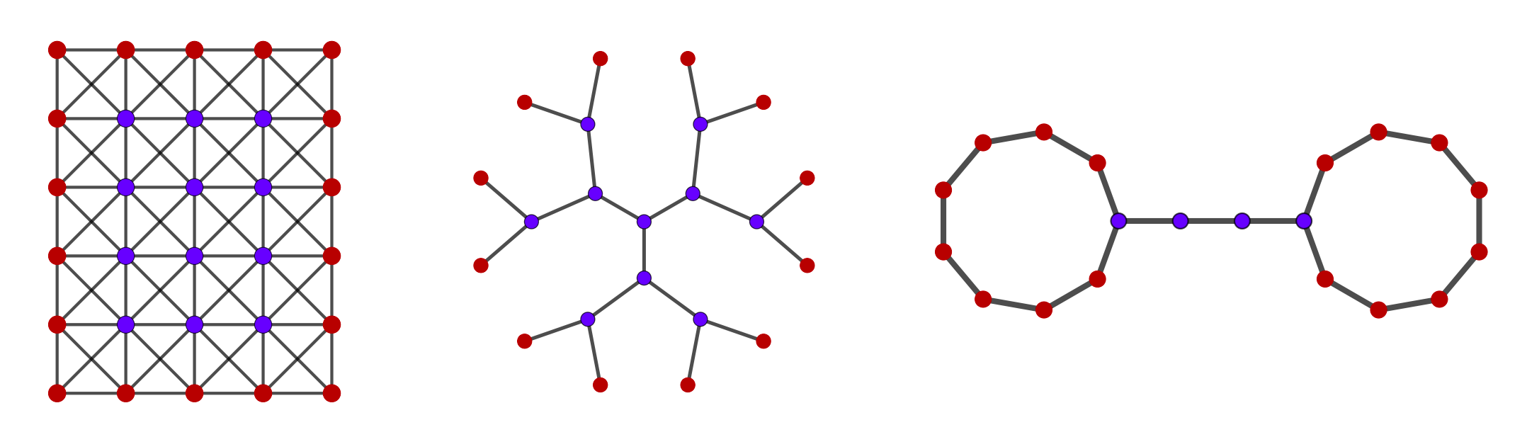
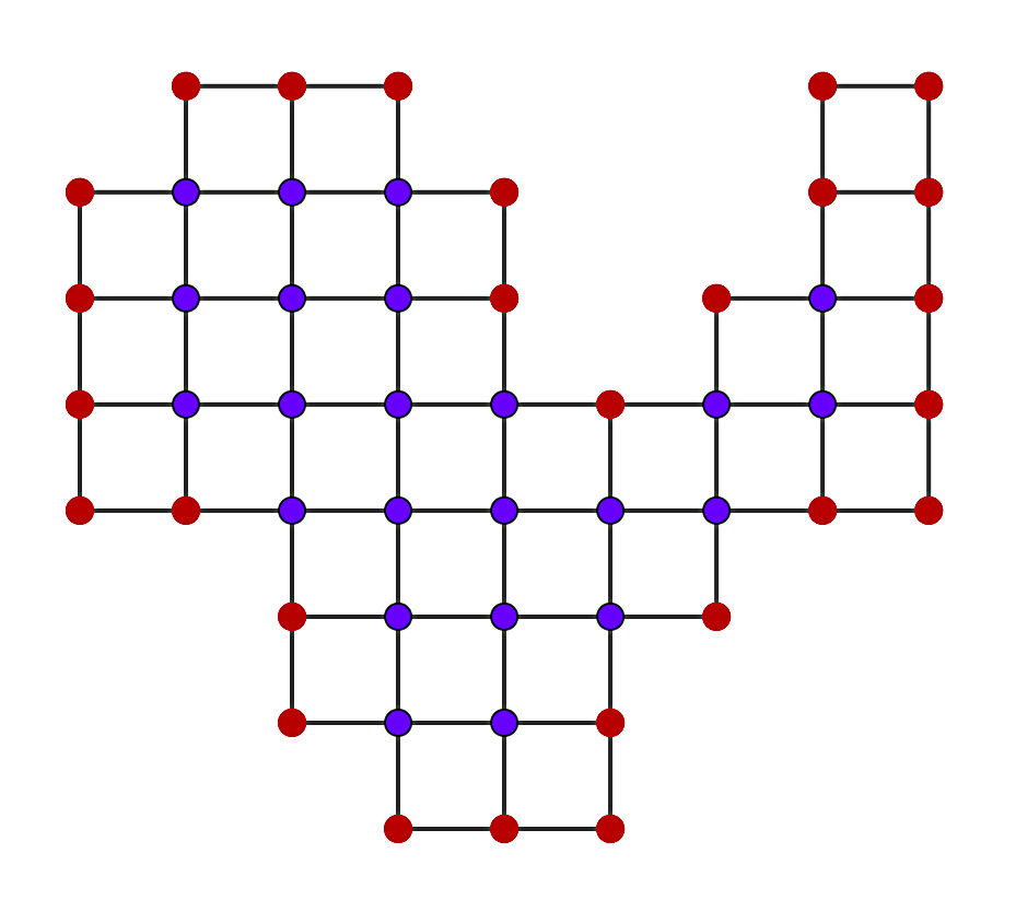
In this section we give notations for the further exposition of the paper. First, we introduce the boundary notion for the connected graphs following the recent work by Steinerberger [21]. The author gives a definition, which coincides with what one would expected for the discretization of (sufficiently nice) Euclidean domains. He also shows an isoperimetric inequality similar to the ones for regular Euclidean domains. Following [21] we set the boundary of a given connected graph $G$ as follows:

$$\partial G=\left\{x\in V\;\Big{|}\;\exists y\in V:\frac{1}{\deg(x)}\sum_{(x,z)\in E}d(z,y)<d(x,y)\right\},$$ (10)

where $G=(V,E),$ $d(x,y)$ is a distance between vertices $x$ and $y.$ By $\deg(x)$ we set the number of neighbor vertices close to $x.$ Note that $\deg(x)=|\{y\in V\;:\;(x,y)\in E\}|.$ Thus, we can easily define the notion of interior points of a graph $G$:

$$G^{o}\equiv V\setminus\partial G.$$

We again follow [21] to depict in Figure $1$ different connected graphs and their boundaries according to a definition given in (10).

Remark 1.

We point out that there are other definitions of a boundary notion for graphs (see for instance [12]), but we consider the above definition due to its natural generalization of regular Euclidean domains boundary properties.

Refer to caption
Refer to caption
Figure 1: Graphs, their boundary $\partial G$ (red) and interior $V\setminus\partial G$ (blue).

We define for a given function $r(x)$ the mean value around $x\in V$ as follows:

$$\overline{r}(x):=\frac{1}{\deg(x)}\sum_{(x,y)\in E}r(y).$$

We set by $u^{l}(x)$ the densities defined on $G,$ also we define the functions $\phi^{l}(x),$ which are defined on $\partial G$ and assume they are extended to be zero on $G^{o},$ for all $l=1,2,\dots,m$. We also impose disjointness condition on $\phi^{l}(x),$ namely $\phi^{i}(x)\cdot\phi^{j}(x)=0,$ for every iβ‰ j,𝑖𝑗i\neq j, and $x\in\partial G.$

According to the above defined densities we will need the following notation as well:

u^t​(x):=ut​(x)βˆ’βˆ‘pβ‰ tup​(x).assignsuperscript^𝑒𝑑π‘₯superscript𝑒𝑑π‘₯subscript𝑝𝑑superscript𝑒𝑝π‘₯\hat{u}^{t}(x):={u}^{t}(x)-\sum\limits_{p\neq t}{u}^{p}(x).

1.4 The setting of the problem and main result

Assume $G=(V,E).$ Let $H(x,s):V\times\mathbb{R}^{+}\to\mathbb{R}$ and $f_{i}(x,s):V\times\mathbb{R}^{+}\to\mathbb{R}$ are continuous in $s,$ and $H(x,0)\equiv 0,f_{i}(x,0)\equiv 0.$ We focus on the following system:

{u1​(x)=max⁑(H​(x,uΒ―1​(x)βˆ’βˆ‘pβ‰ 1uΒ―p​(x))βˆ’f1​(x,u1​(x)), 0),x∈Go,u2​(x)=max⁑(H​(x,uΒ―2​(x)βˆ’βˆ‘pβ‰ 2uΒ―p​(x))βˆ’f2​(x,u2​(x)), 0),x∈Go,…​…​…​…um​(x)=max⁑(H​(x,uΒ―m​(x)βˆ’βˆ‘pβ‰ muΒ―p​(x))βˆ’fm​(x,um​(x)), 0),x∈Go,ul​(x)=Ο•l​(x),xβˆˆβˆ‚G.casesformulae-sequencesuperscript𝑒1π‘₯𝐻π‘₯superscript¯𝑒1π‘₯subscript𝑝1superscript¯𝑒𝑝π‘₯subscript𝑓1π‘₯superscript𝑒1π‘₯ 0π‘₯superscriptπΊπ‘œotherwiseformulae-sequencesuperscript𝑒2π‘₯𝐻π‘₯superscript¯𝑒2π‘₯subscript𝑝2superscript¯𝑒𝑝π‘₯subscript𝑓2π‘₯superscript𝑒2π‘₯ 0π‘₯superscriptπΊπ‘œotherwise…………otherwiseformulae-sequencesuperscriptπ‘’π‘šπ‘₯𝐻π‘₯superscriptΒ―π‘’π‘šπ‘₯subscriptπ‘π‘šsuperscript¯𝑒𝑝π‘₯subscriptπ‘“π‘šπ‘₯superscriptπ‘’π‘šπ‘₯ 0π‘₯superscriptπΊπ‘œotherwiseformulae-sequencesuperscript𝑒𝑙π‘₯superscriptitalic-ϕ𝑙π‘₯π‘₯𝐺otherwise\begin{cases}u^{1}(x)=\max\left(H\left(x,\overline{u}^{1}(x)-\sum\limits_{p\neq 1}\overline{u}^{p}(x)\right)-f_{1}(x,u^{1}(x)),\,0\right),\;\;x\in G^{o},\\ u^{2}(x)=\max\left(H\left(x,\overline{u}^{2}(x)-\sum\limits_{p\neq 2}\overline{u}^{p}(x)\right)-f_{2}(x,u^{2}(x)),\,0\right),\;\;x\in G^{o},\\ \dots\dots\dots\dots\\ u^{m}(x)=\max\left(H\left(x,\overline{u}^{m}(x)-\sum\limits_{p\neq m}\overline{u}^{p}(x)\right)-f_{m}(x,u^{m}(x)),\,0\right),\;\;x\in G^{o},\\ u^{l}(x)=\phi^{l}(x),\;\;x\in\partial G.\end{cases} (11)

for every $l=1,2,\dots,m.$

Remark 2.

Functions $f_{i}$’s are defined only for non negative values of s (recall that densities $u_{i}$’s are non negative due to the above system (11)); thus we can arbitrarily define such functions on the negative semiaxis. For the sake of convenience, when $s\leq 0$, we will let $f_{i}(x,s)=-f_{i}(x,-s)$. This extension preserves the continuity due to the conditions on $f_{i}$ defined above. In the same way, $H$ is extended on the negative semiaxis as well, i.e $H(x,s)=-H(x,-s).$

As special case of (11) let $m=1$ and $f(x)$ be non negative function defined on $V$. The one phase obstacle problem on graph reads as

$$\left\{\begin{array}[]{ll}\min(-{\mathcal{L}}u(x)+f(x),u)=0,&x\in G^{o},\\ u=g,&\text{ on }\partial G,\\ \end{array}\right.$$ (12)

where ${\mathcal{L}}$ is the unnormalized graph Laplacian given by

$$\mathcal{L}u(x_{i})=\sum\limits_{j=1}^{n}\,(u(x_{j})-u(x_{i})).$$

To solve (12) one can rewrite the obstacle problem in the following form

$$u(x)=\max\left(\overline{u}(x)-\frac{1}{\deg(x)}f(x),0\right).$$

The main result of the paper reads as follows:

Theorem 1.

Let the functions $f_{l}(x,s)$ and $H(x,s)$ be nondecreasing with respect to the variable $s$. Assume also that $H$ is a Lipschitz continuous with respect to $s$ and Lipschitz constant is $1,$ i.e. $|H(\cdot,s)-H(\cdot,t)|\leq|s-t|,\forall s,t\in\mathbb{R}^{+}.$ Then there exists a unique vector $(u^{1},u^{2},\dots,u^{m}),$ which satisfies the discrete system (11).

2 Auxiliary lemmas

We start this section by proving that the disjointness condition on $\partial G$ implies the same property for the densities $u^{l}(x)$ over whole graph $G.$ Let $G=(V,E),$ where $V$ is a set of vertices and $E$ is a set of edges to a given graph $G.$

Lemma 1.

Let the functions $f_{l}(x,s)$ and $H(x,s)$ be nondecreasing with respect to the variable $s$. If a vector $(u^{1},u^{2},\dots,u^{m})$ solves the discrete system (11), then the following property holds:

ui​(x)β‹…uj​(x)=0,βˆ€x∈V,iβ‰ j.formulae-sequenceβ‹…superscript𝑒𝑖π‘₯superscript𝑒𝑗π‘₯0formulae-sequencefor-allπ‘₯𝑉𝑖𝑗u^{i}(x)\cdot u^{j}(x)=0,\;\forall x\in V,\;i\neq j.
Proof.

Let $u^{i}(x_{0})>0,$ for some $x_{0}\in G^{o}.$ Then

ui​(x0)=H​(x0,uΒ―i​(x0)βˆ’βˆ‘pβ‰ iuΒ―p​(x0))βˆ’fx0​(x,ui​(x0))>0.superscript𝑒𝑖subscriptπ‘₯0𝐻subscriptπ‘₯0superscript¯𝑒𝑖subscriptπ‘₯0subscript𝑝𝑖superscript¯𝑒𝑝subscriptπ‘₯0subscript𝑓subscriptπ‘₯0π‘₯superscript𝑒𝑖subscriptπ‘₯00u^{i}(x_{0})=H\left(x_{0},\overline{u}^{i}(x_{0})-\sum\limits_{p\neq i}\overline{u}^{p}(x_{0})\right)-f_{x_{0}}(x,u^{i}(x_{0}))>0.

Therefore H​(x0,uΒ―i​(x0)βˆ’βˆ‘pβ‰ iuΒ―p​(x0))>0.𝐻subscriptπ‘₯0superscript¯𝑒𝑖subscriptπ‘₯0subscript𝑝𝑖superscript¯𝑒𝑝subscriptπ‘₯00H\left(x_{0},\overline{u}^{i}(x_{0})-\sum\limits_{p\neq i}\overline{u}^{p}(x_{0})\right)>0. This along with non-decreasing condition on $H$ and $H(x,0)=0,$ implies uΒ―i​(x0)βˆ’βˆ‘pβ‰ iuΒ―p​(x0)β‰₯0.superscript¯𝑒𝑖subscriptπ‘₯0subscript𝑝𝑖superscript¯𝑒𝑝subscriptπ‘₯00\overline{u}^{i}(x_{0})-\sum\limits_{p\neq i}\overline{u}^{p}(x_{0})\geq 0. Thus, for every jβ‰ i𝑗𝑖j\neq i we get uΒ―j​(x0)βˆ’βˆ‘pβ‰ juΒ―p​(x0)≀0.superscript¯𝑒𝑗subscriptπ‘₯0subscript𝑝𝑗superscript¯𝑒𝑝subscriptπ‘₯00\overline{u}^{j}(x_{0})-\sum\limits_{p\neq j}\overline{u}^{p}(x_{0})\leq 0. This apparently yields

H​(x0,uΒ―j​(x0)βˆ’βˆ‘pβ‰ juΒ―p​(x0))≀H​(x0,0)=0,𝐻subscriptπ‘₯0superscript¯𝑒𝑗subscriptπ‘₯0subscript𝑝𝑗superscript¯𝑒𝑝subscriptπ‘₯0𝐻subscriptπ‘₯000H\left(x_{0},\overline{u}^{j}(x_{0})-\sum\limits_{p\neq j}\overline{u}^{p}(x_{0})\right)\leq H(x_{0},0)=0,

hence

uj​(x0)=max⁑(H​(x0,uΒ―j​(x0)βˆ’βˆ‘pβ‰ juΒ―p​(x0))βˆ’fj​(x0,uj​(x0)), 0)=0.superscript𝑒𝑗subscriptπ‘₯0𝐻subscriptπ‘₯0superscript¯𝑒𝑗subscriptπ‘₯0subscript𝑝𝑗superscript¯𝑒𝑝subscriptπ‘₯0subscript𝑓𝑗subscriptπ‘₯0superscript𝑒𝑗subscriptπ‘₯0 00u^{j}(x_{0})=\max\left(H\left(x_{0},\overline{u}^{j}(x_{0})-\sum\limits_{p\neq j}\overline{u}^{p}(x_{0})\right)-f_{j}(x_{0},u^{j}(x_{0})),\,0\right)=0.

This completes the proof.

∎

Lemma 2.

Let the functions $f_{l}(x,s)$ and $H(x,s)$ be nondecreasing with respect to the variable $s$. If a vector $(u^{1},u^{2},\dots,u^{m})$ solves the discrete system (11), then the following inequality holds:

H​(x,uΒ―l​(x)βˆ’βˆ‘pβ‰ luΒ―p​(x))βˆ’u^l​(x)≀fl​(x,ul​(x)),𝐻π‘₯superscript¯𝑒𝑙π‘₯subscript𝑝𝑙superscript¯𝑒𝑝π‘₯superscript^𝑒𝑙π‘₯subscript𝑓𝑙π‘₯superscript𝑒𝑙π‘₯H\left(x,\overline{u}^{l}(x)-\sum\limits_{p\neq l}\overline{u}^{p}(x)\right)-\hat{u}^{l}(x)\leq f_{l}(x,u^{l}(x)),

for all $l=1,2,...,m$ and $x\in V.$

Proof.

Let $u^{l}(x)$ is a fixed density. Assume for some $x_{0}\in G^{o}$ we have $u^{l}(x_{0})>0.$ Then according to Lemma 1 for every pβ‰ l𝑝𝑙p\neq l we obtain $u^{p}(x_{0})=0.$ Hence $\hat{u}^{l}(x_{0})={u}^{l}(x_{0})$ and this in turn gives

H​(x0,uΒ―l​(x0)βˆ’βˆ‘pβ‰ luΒ―p​(x0))βˆ’u^l​(x0)𝐻subscriptπ‘₯0superscript¯𝑒𝑙subscriptπ‘₯0subscript𝑝𝑙superscript¯𝑒𝑝subscriptπ‘₯0superscript^𝑒𝑙subscriptπ‘₯0\displaystyle H\left(x_{0},\overline{u}^{l}(x_{0})-\sum\limits_{p\neq l}\overline{u}^{p}(x_{0})\right)-\hat{u}^{l}(x_{0}) =H​(x0,uΒ―l​(x0)βˆ’βˆ‘pβ‰ luΒ―p​(x0))βˆ’ul​(x0)absent𝐻subscriptπ‘₯0superscript¯𝑒𝑙subscriptπ‘₯0subscript𝑝𝑙superscript¯𝑒𝑝subscriptπ‘₯0superscript𝑒𝑙subscriptπ‘₯0\displaystyle=H\left(x_{0},\overline{u}^{l}(x_{0})-\sum\limits_{p\neq l}\overline{u}^{p}(x_{0})\right)-{u}^{l}(x_{0})
$\displaystyle=f_{l}(x_{0},u^{l}(x_{0})).$

Now let for some $x_{0}\in G^{o}$ we have $u^{l}(x_{0})=0.$ In this case if all $u^{p}(x_{0})=0$ for every $p=1,2,...m,$ then the required inequality follows from the system (11). Assume there exist some tβ‰ l𝑑𝑙t\neq l such that $u^{t}(x_{0})>0.$ In this case recalling again the system (11) and that for $s\leq 0$ we extend $H$ function as $H(x,s)=-H(x,-s),$ we obtain:

H​(x0,uΒ―l​(x0)βˆ’βˆ‘pβ‰ luΒ―p​(x0))βˆ’u^l​(x0)=H​(x0,uΒ―l​(x0)βˆ’βˆ‘pβ‰ luΒ―p​(x0))+ut​(x0)==H​(x0,uΒ―l​(x0)βˆ’βˆ‘pβ‰ luΒ―p​(x0))+H​(x0,uΒ―t​(x0)βˆ’βˆ‘pβ‰ tuΒ―p​(x0))βˆ’ft​(x0,ut​(x0))==H​(x0,uΒ―t​(x0)βˆ’βˆ‘pβ‰ tuΒ―p​(x0))βˆ’H​(x0,βˆ‘pβ‰ luΒ―p​(x0)βˆ’uΒ―l​(x0))βˆ’ft​(x0,ut​(x0)).𝐻subscriptπ‘₯0superscript¯𝑒𝑙subscriptπ‘₯0subscript𝑝𝑙superscript¯𝑒𝑝subscriptπ‘₯0superscript^𝑒𝑙subscriptπ‘₯0𝐻subscriptπ‘₯0superscript¯𝑒𝑙subscriptπ‘₯0subscript𝑝𝑙superscript¯𝑒𝑝subscriptπ‘₯0superscript𝑒𝑑subscriptπ‘₯0𝐻subscriptπ‘₯0superscript¯𝑒𝑙subscriptπ‘₯0subscript𝑝𝑙superscript¯𝑒𝑝subscriptπ‘₯0𝐻subscriptπ‘₯0superscript¯𝑒𝑑subscriptπ‘₯0subscript𝑝𝑑superscript¯𝑒𝑝subscriptπ‘₯0subscript𝑓𝑑subscriptπ‘₯0superscript𝑒𝑑subscriptπ‘₯0𝐻subscriptπ‘₯0superscript¯𝑒𝑑subscriptπ‘₯0subscript𝑝𝑑superscript¯𝑒𝑝subscriptπ‘₯0𝐻subscriptπ‘₯0subscript𝑝𝑙superscript¯𝑒𝑝subscriptπ‘₯0superscript¯𝑒𝑙subscriptπ‘₯0subscript𝑓𝑑subscriptπ‘₯0superscript𝑒𝑑subscriptπ‘₯0H\left(x_{0},\overline{u}^{l}(x_{0})-\sum\limits_{p\neq l}\overline{u}^{p}(x_{0})\right)-\hat{u}^{l}(x_{0})=H\left(x_{0},\overline{u}^{l}(x_{0})-\sum\limits_{p\neq l}\overline{u}^{p}(x_{0})\right)+{u}^{t}(x_{0})=\\ =H\left(x_{0},\overline{u}^{l}(x_{0})-\sum\limits_{p\neq l}\overline{u}^{p}(x_{0})\right)+H\left(x_{0},\overline{u}^{t}(x_{0})-\sum\limits_{p\neq t}\overline{u}^{p}(x_{0})\right)-f_{t}(x_{0},u^{t}(x_{0}))=\\ =H\left(x_{0},\overline{u}^{t}(x_{0})-\sum\limits_{p\neq t}\overline{u}^{p}(x_{0})\right)-H\left(x_{0},\sum\limits_{p\neq l}\overline{u}^{p}(x_{0})-\overline{u}^{l}(x_{0})\right)-f_{t}(x_{0},u^{t}(x_{0})).

It is easy to see that

0≀uΒ―t​(x0)βˆ’βˆ‘pβ‰ tuΒ―p​(x0)β‰€βˆ‘pβ‰ luΒ―p​(x0)βˆ’uΒ―l​(x0),0superscript¯𝑒𝑑subscriptπ‘₯0subscript𝑝𝑑superscript¯𝑒𝑝subscriptπ‘₯0subscript𝑝𝑙superscript¯𝑒𝑝subscriptπ‘₯0superscript¯𝑒𝑙subscriptπ‘₯00\leq\overline{u}^{t}(x_{0})-\sum\limits_{p\neq t}\overline{u}^{p}(x_{0})\leq\sum\limits_{p\neq l}\overline{u}^{p}(x_{0})-\overline{u}^{l}(x_{0}),

hence by the non-decreasing property of $H$ one implies

H​(x0,uΒ―t​(x0)βˆ’βˆ‘pβ‰ tuΒ―p​(x0))βˆ’H​(x0,βˆ‘pβ‰ luΒ―p​(x0)βˆ’uΒ―l​(x0))βˆ’ft​(x0,ut​(x0))β‰€β‰€βˆ’ft​(x0,ut​(x0))≀0≀fl​(x0,ul​(x0)).𝐻subscriptπ‘₯0superscript¯𝑒𝑑subscriptπ‘₯0subscript𝑝𝑑superscript¯𝑒𝑝subscriptπ‘₯0𝐻subscriptπ‘₯0subscript𝑝𝑙superscript¯𝑒𝑝subscriptπ‘₯0superscript¯𝑒𝑙subscriptπ‘₯0subscript𝑓𝑑subscriptπ‘₯0superscript𝑒𝑑subscriptπ‘₯0subscript𝑓𝑑subscriptπ‘₯0superscript𝑒𝑑subscriptπ‘₯00subscript𝑓𝑙subscriptπ‘₯0superscript𝑒𝑙subscriptπ‘₯0H\left(x_{0},\overline{u}^{t}(x_{0})-\sum\limits_{p\neq t}\overline{u}^{p}(x_{0})\right)-H\left(x_{0},\sum\limits_{p\neq l}\overline{u}^{p}(x_{0})-\overline{u}^{l}(x_{0})\right)-f_{t}(x_{0},u^{t}(x_{0}))\leq\\ \leq-f_{t}(x_{0},u^{t}(x_{0}))\leq 0\leq f_{l}(x_{0},u^{l}(x_{0})).

This completes the proof.

∎

Lemma 3.

Let the functions $f_{l}(x,s)$ and $H(x,s)$ be nondecreasing with respect to the variable $s$. Assume also that $H$ is a Lipschitz continuous with respect to $s$ and Lipschitz constant is $1,$ i.e. $|H(\cdot,s)-H(\cdot,t)|\leq|s-t|,\forall s,t\in\mathbb{R}^{+}.$ If any two vectors $(u^{1},u^{2},\dots,u^{m})$ and $(v^{1},v^{2},\dots,v^{m})$ are satisfying the discrete system (11), then the following equation holds:

$$\max_{x\in V}\left(\hat{u}^{l}(x)-\hat{v}^{l}(x)\right)=\max_{\{x\in V\;:\;u^{l}(x)\leq v^{l}(x)\}}\left(\hat{u}^{l}(x)-\hat{v}^{l}(x)\right),$$

for all $l=1,2,\dots,m$.

Proof.

We argue by contradiction. Suppose for some $l_{0}$ we have

$$\begin{multlined}\hat{u}^{l_{0}}(x_{0})-\hat{v}^{l_{0}}(x_{0})=\max_{x\in V}(\hat{u}^{l_{0}}(x)-\hat{v}^{l_{0}}(x))=\\ =\max_{\{x\in V\;:\;u^{l_{0}}(x)>v^{l_{0}}(x)\}}(\hat{u}^{l_{0}}(x)-\hat{v}^{l_{0}}(x))>\max_{\{x\in V\;:\;u^{l_{0}}(x)\leq v^{l_{0}}(x)\}}(\hat{u}_{\alpha}^{l_{0}}(x)-\hat{v}_{\alpha}^{l_{0}}(x)).\end{multlined}\hat{u}^{l_{0}}(x_{0})-\hat{v}^{l_{0}}(x_{0})=\max_{x\in V}(\hat{u}^{l_{0}}(x)-\hat{v}^{l_{0}}(x))=\\ =\max_{\{x\in V\;:\;u^{l_{0}}(x)>v^{l_{0}}(x)\}}(\hat{u}^{l_{0}}(x)-\hat{v}^{l_{0}}(x))>\max_{\{x\in V\;:\;u^{l_{0}}(x)\leq v^{l_{0}}(x)\}}(\hat{u}_{\alpha}^{l_{0}}(x)-\hat{v}_{\alpha}^{l_{0}}(x)).$$ (13)

Then according to Lemma 1 the following simple chain of inclusions hold:

$$\{u^{l}(x)>v^{l}(x)\}\subset\{\hat{u}^{l}(x)>\hat{v}^{l}(x)\}\subset\{u^{l}(x)\geq v^{l}(x)\}.$$ (14)

We obviously see that $u^{l_{0}}(x_{0})>v^{l_{0}}(x_{0})\geq 0$ implies $\hat{u}^{l_{0}}(x_{0})>\hat{v}^{l_{0}}(x_{0})$. On the other hand, the discrete system (11) and Lemma 2 gives us

H​(x0,uΒ―l0​(x0)βˆ’βˆ‘pβ‰ l0uΒ―p​(x0))βˆ’u^l0​(x0)=fl0​(x0,ul0​(x0)),𝐻subscriptπ‘₯0superscript¯𝑒subscript𝑙0subscriptπ‘₯0subscript𝑝subscript𝑙0superscript¯𝑒𝑝subscriptπ‘₯0superscript^𝑒subscript𝑙0subscriptπ‘₯0subscript𝑓subscript𝑙0subscriptπ‘₯0superscript𝑒subscript𝑙0subscriptπ‘₯0H\left(x_{0},\overline{u}^{l_{0}}(x_{0})-\sum\limits_{p\neq l_{0}}\overline{u}^{p}(x_{0})\right)-\hat{u}^{l_{0}}(x_{0})=f_{l_{0}}(x_{0},u^{l_{0}}(x_{0})),

and

H​(x0,vΒ―l0​(x0)βˆ’βˆ‘pβ‰ l0vΒ―p​(x0))βˆ’v^l0​(x0)≀fl0​(x0,vl0​(x0)).𝐻subscriptπ‘₯0superscript¯𝑣subscript𝑙0subscriptπ‘₯0subscript𝑝subscript𝑙0superscript¯𝑣𝑝subscriptπ‘₯0superscript^𝑣subscript𝑙0subscriptπ‘₯0subscript𝑓subscript𝑙0subscriptπ‘₯0superscript𝑣subscript𝑙0subscriptπ‘₯0H\left(x_{0},\overline{v}^{l_{0}}(x_{0})-\sum\limits_{p\neq l_{0}}\overline{v}^{p}(x_{0})\right)-\hat{v}^{l_{0}}(x_{0})\leq f_{l_{0}}(x_{0},v^{l_{0}}(x_{0})).

Therefore

H​(x0,uΒ―l0​(x0)βˆ’βˆ‘pβ‰ l0uΒ―p​(x0))βˆ’H​(x0,vΒ―l0​(x0)βˆ’βˆ‘pβ‰ l0vΒ―p​(x0))βˆ’(u^l0​(x0)βˆ’v^l0​(x0))β‰₯fl0​(x0,ul0​(x0))βˆ’fl0​(x0,vl0​(x0))β‰₯0.𝐻subscriptπ‘₯0superscript¯𝑒subscript𝑙0subscriptπ‘₯0subscript𝑝subscript𝑙0superscript¯𝑒𝑝subscriptπ‘₯0𝐻subscriptπ‘₯0superscript¯𝑣subscript𝑙0subscriptπ‘₯0subscript𝑝subscript𝑙0superscript¯𝑣𝑝subscriptπ‘₯0superscript^𝑒subscript𝑙0subscriptπ‘₯0superscript^𝑣subscript𝑙0subscriptπ‘₯0subscript𝑓subscript𝑙0subscriptπ‘₯0superscript𝑒subscript𝑙0subscriptπ‘₯0subscript𝑓subscript𝑙0subscriptπ‘₯0superscript𝑣subscript𝑙0subscriptπ‘₯00\begin{multlined}H\left(x_{0},\overline{u}^{l_{0}}(x_{0})-\sum\limits_{p\neq l_{0}}\overline{u}^{p}(x_{0})\right)-H\left(x_{0},\overline{v}^{l_{0}}(x_{0})-\sum\limits_{p\neq l_{0}}\overline{v}^{p}(x_{0})\right)\\ -\left(\hat{u}^{l_{0}}(x_{0})-\hat{v}^{l_{0}}(x_{0})\right)\geq f_{l_{0}}(x_{0},u^{l_{0}}(x_{0}))-f_{l_{0}}(x_{0},v^{l_{0}}(x_{0}))\geq 0.\end{multlined}H\left(x_{0},\overline{u}^{l_{0}}(x_{0})-\sum\limits_{p\neq l_{0}}\overline{u}^{p}(x_{0})\right)-H\left(x_{0},\overline{v}^{l_{0}}(x_{0})-\sum\limits_{p\neq l_{0}}\overline{v}^{p}(x_{0})\right)\\ -\left(\hat{u}^{l_{0}}(x_{0})-\hat{v}^{l_{0}}(x_{0})\right)\geq f_{l_{0}}(x_{0},u^{l_{0}}(x_{0}))-f_{l_{0}}(x_{0},v^{l_{0}}(x_{0}))\geq 0.

Thus using non-decreasing and Lipschitz properties of $H$, we conclude

$\displaystyle 0<\left(\hat{u}^{l_{0}}(x_{0})-\hat{v}^{l_{0}}(x_{0})\right)$ ≀H​(x0,uΒ―l0​(x0)βˆ’βˆ‘pβ‰ l0uΒ―p​(x0))βˆ’H​(x0,vΒ―l0​(x0)βˆ’βˆ‘pβ‰ l0vΒ―p​(x0))absent𝐻subscriptπ‘₯0superscript¯𝑒subscript𝑙0subscriptπ‘₯0subscript𝑝subscript𝑙0superscript¯𝑒𝑝subscriptπ‘₯0𝐻subscriptπ‘₯0superscript¯𝑣subscript𝑙0subscriptπ‘₯0subscript𝑝subscript𝑙0superscript¯𝑣𝑝subscriptπ‘₯0\displaystyle\leq H\left(x_{0},\overline{u}^{l_{0}}(x_{0})-\sum\limits_{p\neq l_{0}}\overline{u}^{p}(x_{0})\right)-H\left(x_{0},\overline{v}^{l_{0}}(x_{0})-\sum\limits_{p\neq l_{0}}\overline{v}^{p}(x_{0})\right) (15)
≀(uΒ―l0​(x0)βˆ’βˆ‘pβ‰ l0uΒ―p​(x0))βˆ’(vΒ―l0​(x0)βˆ’βˆ‘pβ‰ l0vΒ―p​(x0))absentsuperscript¯𝑒subscript𝑙0subscriptπ‘₯0subscript𝑝subscript𝑙0superscript¯𝑒𝑝subscriptπ‘₯0superscript¯𝑣subscript𝑙0subscriptπ‘₯0subscript𝑝subscript𝑙0superscript¯𝑣𝑝subscriptπ‘₯0\displaystyle\leq\left(\overline{u}^{l_{0}}(x_{0})-\sum\limits_{p\neq l_{0}}\overline{u}^{p}(x_{0})\right)-\left(\overline{v}^{l_{0}}(x_{0})-\sum\limits_{p\neq l_{0}}\overline{v}^{p}(x_{0})\right)
$\displaystyle=\frac{1}{\deg(x_{0})}\sum_{(x_{0},y)\in E}\left(\hat{u}^{l_{0}}(y)-\hat{u}^{l_{0}}(y)\right),$

which implies that $\hat{u}^{l_{0}}(x_{0})-\hat{v}^{l_{0}}(x_{0})=\hat{u}^{l_{0}}(y)-\hat{v}^{l_{0}}(y)>0,$ for all $(x_{0},y)\in E.$ Due to the chain (14), we apparently have ${u}^{l_{0}}(y)\geq{v}^{l_{0}}(y)$. According to our assumption (13), the only possibility is ${u}^{l_{0}}(y)>{v}^{l_{0}}(y)$ for all $(x_{0},y)\in E.$ Now we can proceed the previous steps for all $y\in V$ such that $(x_{0},y)\in E,$ and then for each one we will get corresponding neighbours with the same strict inequality and so on. Since the graph $G$ is connected, then one can always find a path from a given vertex $y$ to the vertex belonging $\partial G.$ Continuing above procedure along this path we will finally approach to the boundary $\partial G$ where as we know ${u}^{l_{0}}(x)={v}^{l_{0}}(x)=\phi^{l_{0}}(x)$ for all $x\in\partial G$. Hence, the strict inequality fails, which implies that our initial assumption (13) is false. Observe that the same arguments can be applied if we interchange the roles of ${u}^{l}(x)$ and ${v}^{l}(x)$. Thus, we also have

$$\max_{G}\left(\hat{v}^{l}(x)-\hat{u}^{l}(x)\right)=\max_{\{v^{l}(x)\leq u^{l}(x)\}}\left(\hat{v}^{l}(x)-\hat{u}^{l}(x)\right),$$

for every $l=1,2,\dots,m$.

Particularly, for every fixed $l=1,2.\dots,m$ and $x\in V$ we have

$$-\max_{\{v^{l}(x)\leq u^{l}(x)\}}(\hat{v}^{l}(x)-\hat{u}^{l}(x))=-\max\limits_{x\in V}(\hat{v}^{l}(x)-\hat{u}^{l}(x))\leq\\ \leq\hat{u}^{l}(x)-\hat{v}^{l}(x)\leq\max\limits_{x\in V}(\hat{u}^{l}(x)-\hat{v}^{l}(x))=\max_{\{u^{l}(x)\leq v^{l}(x)\}}(\hat{u}^{l}(x)-\hat{v}^{l}(x)).$$ (16)

∎

Thanks to Lemma 3 in the sequel we will use the following notations:

$$A:=\max_{l}\;\left(\max\limits_{x\in V}(\hat{u}^{l}(x)-\hat{v}^{l}(x))\right)=\max_{l}\;\left(\max\limits_{\{u^{l}(x)\leq v^{l}(x)\}}(\hat{u}^{l}(x)-\hat{v}^{l}(x))\right),$$

and

$$B:=\max_{l}\;\left(\max\limits_{x\in V}(\hat{v}^{l}(x)-\hat{u}^{l}(x))\right)=\max_{l}\;\left(\max\limits_{\{v^{l}(x)\leq u^{l}(x)\}}(\hat{v}^{l}(x)-\hat{u}^{l}(x))\right).$$
Lemma 4.

Let the functions $f_{l}(x,s)$ and $H(x,s)$ be nondecreasing with respect to the variable $s$. Assume also that $H$ is a Lipschitz continuous with respect to $s$ and Lipschitz constant is $1,$ i.e. $|H(\cdot,s)-H(\cdot,t)|\leq|s-t|,\forall s,t\in\mathbb{R}^{+}.$ Let two vectors $(u^{1},u^{2},\dots,u^{m})$ and $(v^{1},v^{2},\dots,v^{m})$ be solving the discrete system (11). For them we set $A$ and $B$ as defined above. If $A>0$ and it is attained for some $l_{0}$, then $A=B>0$ and there exists some t0β‰ l0,subscript𝑑0subscript𝑙0t_{0}\neq l_{0}, and $y_{0}\in V,$ such that

$$0<A=\max_{\{u^{l_{0}}(x)\leq v^{l_{0}}(x)\}}(\hat{u}^{l_{0}}(x)-\hat{v}^{l_{0}}(x))=\max_{\{u^{l_{0}}(x)=v^{l_{0}}(x)=0\}}(\hat{u}^{l_{0}}(x)-\hat{v}^{l_{0}}(x))=\hat{v}^{t_{0}}(y_{0})-\hat{u}^{t_{0}}(y_{0}).$$
Proof.

Due to disjointness property of densities $u^{l}$ and $v^{l}$ (see Lemma 1) We easily observe that $(\hat{u}^{l_{0}}(x)-\hat{v}^{l_{0}}(x))$ might be positive only on the set $\{u^{l_{0}}(x)=v^{l_{0}}(x)=0\}$ (because for the other cases simple checking provides $(\hat{u}^{l_{0}}(x)-\hat{v}^{l_{0}}(x))\leq 0)$. Hence,

$$A=\max_{\{u^{l_{0}}(x)=v^{l_{0}}(x)=0\}}(\hat{u}^{l_{0}}(x)-\hat{v}^{l_{0}}(x)).$$

Using the latter equality, one can prove that $A>0$ implies $B>0$. Indeed, if we assume that $B\leq 0,$ then according to definition of $B$ we will get that $\hat{v}^{l}(x)\leq\hat{u}^{l}(x)$ for all $l=\overline{1,m}$ and $x\in V$. This obviously yields ${v}^{l}(x)\leq{u}^{l}(x),$ for all $l=\overline{1,m}$ and $x\in V$. Thus,

0<A=max{ul0​(x)=vl0​(x)=0}⁑(u^l0​(x)βˆ’v^l0​(x))=max{ul0​(x)=vl0​(x)=0}⁑(βˆ‘lβ‰ l0(vl​(x)βˆ’ul​(x)))≀0.0𝐴subscriptsuperscript𝑒subscript𝑙0π‘₯superscript𝑣subscript𝑙0π‘₯0superscript^𝑒subscript𝑙0π‘₯superscript^𝑣subscript𝑙0π‘₯subscriptsuperscript𝑒subscript𝑙0π‘₯superscript𝑣subscript𝑙0π‘₯0subscript𝑙subscript𝑙0superscript𝑣𝑙π‘₯superscript𝑒𝑙π‘₯00<A=\max_{\{u^{l_{0}}(x)=v^{l_{0}}(x)=0\}}(\hat{u}^{l_{0}}(x)-\hat{v}^{l_{0}}(x))=\max_{\{u^{l_{0}}(x)=v^{l_{0}}(x)=0\}}\left(\sum_{l\neq l_{0}}(v^{l}(x)-u^{l}(x))\right)\leq 0.

This is a contradiction, and therefore $B>0$. It is clear that in a similar way one can prove the converse statement as well. Thus, we clearly see that at the same time either both $A$ and $B$ are non-positive, or they are positive.

Concerning the equality $A=B,$ it is easy to see that if the maximum $A>0$ is attained at vertex $y_{0}\in V,$ then the following holds:

0<A=max{ul0​(x)=vl0​(x)=0}⁑(u^l0​(x)βˆ’v^l0​(x))=u^l0​(y0)βˆ’v^l0​(y0)=βˆ‘lβ‰ l0(vl​(y0)βˆ’ul​(y0)).0𝐴subscriptsuperscript𝑒subscript𝑙0π‘₯superscript𝑣subscript𝑙0π‘₯0superscript^𝑒subscript𝑙0π‘₯superscript^𝑣subscript𝑙0π‘₯superscript^𝑒subscript𝑙0subscript𝑦0superscript^𝑣subscript𝑙0subscript𝑦0subscript𝑙subscript𝑙0superscript𝑣𝑙subscript𝑦0superscript𝑒𝑙subscript𝑦00<A=\max_{\{u^{l_{0}}(x)=v^{l_{0}}(x)=0\}}(\hat{u}^{l_{0}}(x)-\hat{v}^{l_{0}}(x))=\hat{u}^{l_{0}}(y_{0})-\hat{v}^{l_{0}}(y_{0})=\sum_{l\neq l_{0}}(v^{l}(y_{0})-u^{l}(y_{0})).

The above result implies that βˆ‘lβ‰ l0vl​(y0)subscript𝑙subscript𝑙0superscript𝑣𝑙subscript𝑦0\sum_{l\neq l_{0}}v^{l}(y_{0}) is strictly positive, therefore there exists t0β‰ l0subscript𝑑0subscript𝑙0t_{0}\neq l_{0} such that ${v}^{t_{0}}(y_{0})>0,$ which in turn allows to write ${v}^{t_{0}}(y_{0})=\hat{v}^{t_{0}}(y_{0})$. Hence,

0<A=vt0​(y0)βˆ’βˆ‘lβ‰ l0ul​(y0)≀v^t0​(y0)βˆ’ut0​(y0)+βˆ‘lβ‰ t0ul​(y0)=v^t0​(y0)βˆ’u^t0​(y0)≀B.0𝐴superscript𝑣subscript𝑑0subscript𝑦0subscript𝑙subscript𝑙0superscript𝑒𝑙subscript𝑦0superscript^𝑣subscript𝑑0subscript𝑦0superscript𝑒subscript𝑑0subscript𝑦0subscript𝑙subscript𝑑0superscript𝑒𝑙subscript𝑦0superscript^𝑣subscript𝑑0subscript𝑦0superscript^𝑒subscript𝑑0subscript𝑦0𝐡0<A={v}^{t_{0}}(y_{0})-\sum_{l\neq l_{0}}{u}^{l}(y_{0})\leq\hat{v}^{t_{0}}(y_{0})-u^{t_{0}}(y_{0})+\sum_{l\neq t_{0}}u^{l}(y_{0})=\hat{v}^{t_{0}}(y_{0})-\hat{u}^{t_{0}}(y_{0})\leq B. (17)

In the same way we will obtain that $B\leq A,$ and therefore $A=B$. On the other hand, since $A=B,$ then the following obvious equality holds

A=vt0​(y0)βˆ’βˆ‘lβ‰ l0ul​(y0)=v^t0​(y0)βˆ’u^t0​(y0)=B.𝐴superscript𝑣subscript𝑑0subscript𝑦0subscript𝑙subscript𝑙0superscript𝑒𝑙subscript𝑦0superscript^𝑣subscript𝑑0subscript𝑦0superscript^𝑒subscript𝑑0subscript𝑦0𝐡A={v}^{t_{0}}(y_{0})-\sum_{l\neq l_{0}}{u}^{l}(y_{0})=\hat{v}^{t_{0}}(y_{0})-\hat{u}^{t_{0}}(y_{0})=B.

This completes the proof. ∎

3 Proof of Theorem 1

Proof.

Let two vectors $(u^{1},u^{2},\dots,u^{m})$ and $(v^{1},v^{2},\dots,v^{m})$ be solving the discrete system (11). For these vectors we set the definition of $A$ and $B$. Then, we consider two cases $A\leq 0$ and $A>0$. If we assume that $A\leq 0,$ then according to Lemma 4, we get $B\leq 0$. But if $A$ and $B$ are non-positive, then the uniqueness follows. Indeed, due to (16) we have the following obvious inequalities

$$0\leq-B\leq\hat{u}^{l}(x)-\hat{v}^{l}(x)\leq A\leq 0.$$

This provides for every $l=\overline{1,m}$ and $x\in V$ we have $\hat{u}^{l}(x)=\hat{v}^{l}(x),$ which in turn implies

$${u}^{l}(x)={v}^{l}(x).$$

Now suppose $A>0$. Our aim is to prove that this case leads to a contradiction. Let the value $A$ is attained for some $l_{0}\in\overline{1,m},$ then due to Lemma 4 there exist $y_{0}\in V$ and t0β‰ l0subscript𝑑0subscript𝑙0t_{0}\neq l_{0} such that:

$\displaystyle 0<A=B=$ $\displaystyle\max_{\{u^{l_{0}}(x)\leq v^{l_{0}}(x)\}}(\hat{u}^{l_{0}}(x)-\hat{v}^{l_{0}}(x))$
$\displaystyle=\max_{\{u^{l_{0}}(x)=v^{l_{0}}(x)=0\}}(\hat{u}^{l_{0}}(x)-\hat{v}^{l_{0}}(x))=\hat{v}^{t_{0}}(y_{0})-\hat{u}^{t_{0}}(y_{0}).$

According to Lemma 2 we have

H​(y0,vΒ―t0​(y0)βˆ’βˆ‘pβ‰ t0vΒ―p​(y0))βˆ’v^t0​(y0)=ft0​(y0,vt0​(y0)),𝐻subscript𝑦0superscript¯𝑣subscript𝑑0subscript𝑦0subscript𝑝subscript𝑑0superscript¯𝑣𝑝subscript𝑦0superscript^𝑣subscript𝑑0subscript𝑦0subscript𝑓subscript𝑑0subscript𝑦0superscript𝑣subscript𝑑0subscript𝑦0H\left(y_{0},\overline{v}^{t_{0}}(y_{0})-\sum\limits_{p\neq t_{0}}\overline{v}^{p}(y_{0})\right)-\hat{v}^{t_{0}}(y_{0})=f_{t_{0}}(y_{0},v^{t_{0}}(y_{0})),

and

H​(y0,uΒ―t0​(y0)βˆ’βˆ‘pβ‰ t0uΒ―p​(y0))βˆ’u^t0​(y0)≀ft0​(y0,ut0​(y0)).𝐻subscript𝑦0superscript¯𝑒subscript𝑑0subscript𝑦0subscript𝑝subscript𝑑0superscript¯𝑒𝑝subscript𝑦0superscript^𝑒subscript𝑑0subscript𝑦0subscript𝑓subscript𝑑0subscript𝑦0superscript𝑒subscript𝑑0subscript𝑦0H\left(y_{0},\overline{u}^{t_{0}}(y_{0})-\sum\limits_{p\neq t_{0}}\overline{u}^{p}(y_{0})\right)-\hat{u}^{t_{0}}(y_{0})\leq f_{t_{0}}(y_{0},u^{t_{0}}(y_{0})).

Recalling that $f_{l}(x,s)$ and $H(x,s)$ are non-decreasing with respect to the variable $s$, also $H$ is a Lipschitz continuous w.r.t. $s,$ along with the fact that $\hat{v}^{t_{0}}(y_{0})>\hat{u}^{t_{0}}(y_{0})$ implies ${v}^{t_{0}}(y_{0})\geq{u}^{t_{0}}(y_{0}),$ we can repeat the same steps as in (15) to obtain

$$\left(\hat{v}^{t_{0}}(y_{0})-\hat{u}^{t_{0}}(y_{0})\right)\leq\frac{1}{\deg(y_{0})}\sum_{(y_{0},z)\in E}\left(\hat{v}^{t_{0}}(z)-\hat{u}^{t_{0}}(z)\right).$$

This implies $A=\hat{v}^{t_{0}}(y_{0})-\hat{u}^{t_{0}}(y_{0})=\hat{v}^{t_{0}}(z)-\hat{u}^{t_{0}}(z)>0$ for all $(y_{0},z)\in E$. The chain (14) provides that for all $(y_{0},z)\in E,$ we have ${v}^{t_{0}}(z)\geq{u}^{t_{0}}(z)$. Since a graph $G$ is connected, then one can always find a path from $y_{0}$ to some boundary vertex $w\in\partial G.$ Assume the vertices along this path are $y_{0};y_{1};\dots;y_{k-1};y_{k}=w.$ Hence, for every $0\leq j\leq k-1,$ we have $(y_{j},y_{j+1})\in E,$ i.e. every vertex $y_{j+1}$ is a closest neighbor for $y_{j}$ and $y_{j+2}.$

According to the above arguments for the neighbor vertex $y_{1}\in V$ we proceed as follows: If ${v}^{t_{0}}(y_{1})>{u}^{t_{0}}(y_{1}),$ then obviously

$$\left(\hat{v}^{t_{0}}(y_{1})-\hat{u}^{t_{0}}(y_{1})\right)\leq\frac{1}{\deg(y_{1})}\sum_{(y_{1},z)\in E}\left(\hat{v}^{t_{0}}(z)-\hat{u}^{t_{0}}(z)\right).$$

This, as we saw a few lines above, leads to $A=\hat{v}^{t_{0}}(y_{1})-\hat{u}^{t_{0}}(y_{1})=\hat{v}^{t_{0}}(z)-\hat{u}^{t_{0}}(z)>0$ for all $(y_{1},z)\in E$. In particular, $A=\hat{v}^{t_{0}}(y_{2})-\hat{u}^{t_{0}}(y_{2})>0.$

If ${v}^{t_{0}}(y_{1})={u}^{t_{0}}(y_{1}),$ then due to $\hat{v}^{t_{0}}(y_{1})-\hat{u}^{t_{0}}(y_{1})=A=B>0,$ there exists some Ξ»0β‰ t0,subscriptπœ†0subscript𝑑0\lambda_{0}\neq t_{0}, such that

0<A=v^t0​(y1)βˆ’u^t0​(y1)=βˆ‘lβ‰ t0(ul​(y1)βˆ’vl​(y1))=uΞ»0​(y1)βˆ’βˆ‘lβ‰ t0vl​(y1).0𝐴superscript^𝑣subscript𝑑0subscript𝑦1superscript^𝑒subscript𝑑0subscript𝑦1subscript𝑙subscript𝑑0superscript𝑒𝑙subscript𝑦1superscript𝑣𝑙subscript𝑦1superscript𝑒subscriptπœ†0subscript𝑦1subscript𝑙subscript𝑑0superscript𝑣𝑙subscript𝑦10<A=\hat{v}^{t_{0}}(y_{1})-\hat{u}^{t_{0}}(y_{1})=\sum_{l\neq t_{0}}\left({u}^{l}(y_{1})-{v}^{l}(y_{1})\right)={u}^{\lambda_{0}}(y_{1})-\sum_{l\neq t_{0}}{v}^{l}(y_{1}).

Note that ${u}^{\lambda_{0}}(y_{1})>0$ implies ${u}^{l}(y_{1})=0$ for all lβ‰ Ξ»0,𝑙subscriptπœ†0l\neq\lambda_{0}, and particularly ${v}^{t_{0}}(y_{1})={u}^{t_{0}}(y_{1})=0.$ Following the definition of $A,$ we get

A=uΞ»0​(y1)βˆ’βˆ‘lβ‰ t0vl​(y1)β‰₯u^Ξ»0​(y1)βˆ’v^Ξ»0​(y1),𝐴superscript𝑒subscriptπœ†0subscript𝑦1subscript𝑙subscript𝑑0superscript𝑣𝑙subscript𝑦1superscript^𝑒subscriptπœ†0subscript𝑦1superscript^𝑣subscriptπœ†0subscript𝑦1A={u}^{\lambda_{0}}(y_{1})-\sum_{l\neq t_{0}}{v}^{l}(y_{1})\geq\hat{u}^{\lambda_{0}}(y_{1})-\hat{v}^{\lambda_{0}}(y_{1}),

which in turn gives 2β€‹βˆ‘lβ‰ Ξ»0vl​(y1)≀0,2subscript𝑙subscriptπœ†0superscript𝑣𝑙subscript𝑦102\sum\limits_{l\neq\lambda_{0}}{v}^{l}(y_{1})\leq 0, and therefore ${v}^{l}(y_{1})=0$ for all lβ‰ Ξ»0𝑙subscriptπœ†0l\neq\lambda_{0}. Hence

A=uΞ»0​(y1)βˆ’βˆ‘lβ‰ t0vl​(y1)=u^Ξ»0​(y1)βˆ’v^Ξ»0​(y1),𝐴superscript𝑒subscriptπœ†0subscript𝑦1subscript𝑙subscript𝑑0superscript𝑣𝑙subscript𝑦1superscript^𝑒subscriptπœ†0subscript𝑦1superscript^𝑣subscriptπœ†0subscript𝑦1A={u}^{\lambda_{0}}(y_{1})-\sum_{l\neq t_{0}}{v}^{l}(y_{1})=\hat{u}^{\lambda_{0}}(y_{1})-\hat{v}^{\lambda_{0}}(y_{1}),

This suggests us to apply the same approach as above to arrive at

$$\left(\hat{v}^{\lambda_{0}}(y_{1})-\hat{u}^{\lambda_{0}}(y_{1})\right)\leq\frac{1}{\deg(y_{1})}\sum_{(y_{1},z)\in E}\left(\hat{v}^{\lambda_{0}}(z)-\hat{u}^{\lambda_{0}}(z)\right),$$

which leads to $A=\hat{u}^{\lambda_{0}}(y_{1})-\hat{v}^{\lambda_{0}}(y_{1})=\hat{u}^{\lambda_{0}}(z)-\hat{v}^{\lambda_{0}}(z)>0,$ for all $(y_{1},z)\in E$. In particular, $A=\hat{u}^{\lambda_{0}}(y_{2})-\hat{v}^{\lambda_{0}}(y_{2})>0.$ Thus, combining two cases we observe that for $y_{2}\in V$ there exist an index $1\leq l_{y_{2}}\leq m$ (in our case $l_{y_{2}}=t_{0}$ or $l_{y_{2}}=\lambda_{0}$) such that

$$\mbox{either}\;\;\hat{u}^{l_{y_{2}}}(y_{2})-\hat{v}^{l_{y_{2}}}(y_{2})=A,\;\;\mbox{or}\;\;\hat{u}^{l_{y_{2}}}(y_{2})-\hat{v}^{l_{y_{2}}}(y_{2})=-A.$$ (18)

It is not hard to understand that the same procedure can be repeated for a vertex $y_{2}$ instead of $y_{1}$ and come to the same conclusion (18) for $y_{3}\in V$ and some index $l_{y_{3}}$ and so on. This allows to claim that for every $y_{j}\in V$ along the path $(y_{0},\dots,y_{k})$ there exist some $l_{y_{j}}$ such that

$$|\hat{u}^{l_{y_{j}}}(y_{j})-\hat{v}^{l_{y_{j}}}(y_{j})|=A>0.$$

But this means that above equality holds also for $y_{k}=w\in\partial G,$ which will lead to a contradiction, because for every $z\in\partial G,$ and $l=\overline{1,m}$ one has $\hat{u}^{l}(z)-\hat{v}^{l}(z)=0$. This completes the proof. ∎

Thus, the system (11) has a unique solution. Hence, one can think of constructing an iterative method which will converge to the unique solution. To this aim, in the forthcoming work the authors are going to develop the efficient iterative methods to solve the systems of type (11).

Acknowledgments

F. Bozorgnia was supported by the Portuguese National Science Foundation through FCT fellowships and by European Unions Horizon 2020 research and innovation program under Marie SkΕ‚odowska-Curie grant agreement No. 777826 (NoMADS).

References

  • [1] AΒ Arakelyan and FΒ Bozorgnia. Uniqueness of limiting solution to a strongly competing system. Electronic Journal of Differential Equations, 2017:96–96, 2017.
  • [2] Avetik Arakelyan. Convergence of the finite difference scheme for a general class of the spatial segregation of reaction–diffusion systems. Computers & Mathematics with Applications, 75(12):4232–4240, 2018.
  • [3] Avetik Arakelyan and Rafayel Barkhudaryan. A numerical approach for a general class of the spatial segregation of reaction–diffusion systems arising in population dynamics. Computers & Mathematics with Applications, 72(11):2823–2838, 2016.
  • [4] Avetik Arakelyan and Henrik Shahgholian. Multi-phase quadrature domains and a related minimization problem. Potential Analysis, 45(1):135–155, 2016.
  • [5] Farid Bozorgnia. Numerical algorithm for spatial segregation of competitive systems. SIAM J. Sci. Comput., 31(5):3946–3958, 2009.
  • [6] Farid Bozorgnia. Optimal partitions for first eigenvalues of the laplace operator. Numerical Methods for Partial Differential Equations, 31(3):923–949, 2015.
  • [7] Farid Bozorgnia and Avetik Arakelyan. Numerical algorithms for a variational problem of the spatial segregation of reaction–diffusion systems. Applied Mathematics and Computation, 219(17):8863–8875, 2013.
  • [8] Farid Bozorgnia, Morteza Fotouhi, Avetik Arakelyan, and Abderrahim Elmoataz. Graph based semi-supervised learning using spatial segregation theory. arXiv preprint arXiv:2211.16030, 2022.
  • [9] Dorin Bucur and Bozhidar Velichkov. Multiphase shape optimization problems. SIAM Journal on Control and Optimization, 52(6):3556–3591, 2014.
  • [10] LAΒ Caffarelli, ALΒ Karakhanyan, and Fang-Hua Lin. The geometry of solutions to a segregation problem for nondivergence systems. Journal of Fixed Point Theory and Applications, 5(2):319–351, 2009.
  • [11] LuisΒ A Cafferelli and FangΒ Hua Lin. An optimal partition problem for eigenvalues. Journal of scientific Computing, 31(1-2):5–18, 2007.
  • [12] Gary Chartrand, David Erwin, GarryΒ L Johns, and Ping Zhang. Boundary vertices in graphs. Discrete Mathematics, 263(1-3):25–34, 2003.
  • [13] Monica Conti, Susanna Terracini, and G.Β Verzini. Asymptotic estimates for the spatial segregation of competitive systems. Adv. Math., 195(2):524–560, 2005.
  • [14] Monica Conti, Susanna Terracini, and Gianmaria Verzini. An optimal partition problem related to nonlinear eigenvalues. Journal of Functional Analysis, 198(1):160–196, 2003.
  • [15] Monica Conti, Susanna Terracini, and Gianmaria Verzini. A variational problem for the spatial segregation of reaction-diffusion systems. Indiana Univ. Math. J., 54(3):779–815, 2005.
  • [16] E.Β C.Β M. Crooks, E.Β N. Dancer, and D.Β Hilhorst. Fast reaction limit and long time behavior for a competition-diffusion system with Dirichlet boundary conditions. Discrete Contin. Dyn. Syst. Ser. B, 8(1):39–44 (electronic), 2007.
  • [17] E.Β N. Dancer and Zhitao Zhang. Dynamics of Lotka-Volterra competition systems with large interaction. J. Differential Equations, 182(2):470–489, 2002.
  • [18] Norman Dancer. Competing species systems with diffusion and large interactions. Rend. Sem. Mat. Fis. Milano, 65:23–33, 1995.
  • [19] Martin Loebl. Introduction to Graph Theory, pages 13–49. Vieweg+Teubner, Wiesbaden, 2010.
  • [20] Marco Squassina. On the long term spatial segregation for a competition-diffusion system. Asymptot. Anal., 57(1-2):83–103, 2008.
  • [21] Stefan Steinerberger. The boundary of a graph and its isoperimetric inequality. arXiv preprint arXiv:2201.03489, 2022.
  • [22] NicolasΒ Garcia Trillos and Dejan Slepčev. A variational approach to the consistency of spectral clustering. Applied and Computational Harmonic Analysis, 45(2):239–281, 2018.
  • [23] Ulrike von Luxburg. A tutorial on spectral clustering. statistics and computing. Data Structures and Algorithms (cs. DS); Machine Learning, pages 395–416.
  • [24] Dominique Zosso and Braxton Osting. A minimal surface criterion for graph partitioning. Inverse Problems & Imaging, 10(4):1149, 2016.