Tensor rank reduction via coordinate flows

Abstract

Recently, there has been a growing interest in efficient numerical algorithms based on tensor networks and low-rank techniques to approximate high-dimensional functions and solutions to high-dimensional PDEs. In this paper, we propose a new tensor rank reduction method based on coordinate transformations that can greatly increase the efficiency of high-dimensional tensor approximation algorithms. The idea is simple: given a multivariate function, determine a coordinate transformation so that the function in the new coordinate system has smaller tensor rank. We restrict our analysis to linear coordinate transformations, which gives rise to a new class of functions that we refer to as tensor ridge functions. Leveraging Riemannian gradient descent on matrix manifolds we develop an algorithm that determines a quasi-optimal linear coordinate transformation for tensor rank reduction. The results we present for rank reduction via linear coordinate transformations open the possibility for generalizations to larger classes of nonlinear transformations. Numerical applications are presented and discussed for linear and nonlinear PDEs.

1 Introduction

There has been a growing interest in efficient numerical algorithms based on tensor networks and low-rank techniques to approximate high-dimensional functions and solutions to high-dimensional PDEs [25, 8, 22, 23, 45, 47]. A tensor network is a factorization of an entangled object such as a multivariate function or an operator, into a set of simpler objects (e.g., low-dimensional functions or operators) which are amenable to efficient representation and computation. The process of building a tensor network relies on a hierarchical decomposition of the entangled object, which, can be visualized in terms of trees [43, 14, 4]. Such a decomposition is rooted in the spectral theory for linear operators [21], and it opens the possibility to approximate high-dimensional functions and compute the solution of high-dimensional PDEs at a cost that scales linearly with respect to the dimension of the object and polynomially with respect to the tensor rank.

Given the fundamental importance of tensor rank in computations and its non-favorable scaling, in this paper we propose a new tensor rank reduction method based on coordinate flows that can greatly increase the efficiency of high-dimensional tensor approximation algorithms. To describe the method, consider the scalar field $u(\bm{x})$, where $\bm{x}\in\Omega\subseteq\mathbb{R}^{d}$, $d>1$. The idea is very simple: determine an invertible coordinate transformation $\bm{H}:\mathbb{R}^{d}\to\mathbb{R}^{d}$ so that the function

$$v(\bm{x})=u(\bm{H}(\bm{x}))$$ (1)

has smaller tensor rank than $u(\bm{x})$. Representing a function on a transformed coordinate system has proven to be a successful technique for a wide range of applications [29, 44, 19], including tensor rank reduction in quantum many-body problems [26]. To illustrate the effects of coordinate transformations on tensor rank, in Figure 1 we show that a simple two-dimensional rotation can increase the rank of fully separated (i.e., rank one) Gaussian function significantly. Vice versa, the inverse rotation can transform a rotated Gaussian with high tensor rank into a rank one function. Similar results hold of course in higher dimensions.

Under mild assumptions on the function $u(\bm{x})$, one may argue, e.g. using nonlinear dynamics or the theory of optimal mass transport, that there always exists a transformation $\bm{H}$ such that $v(\bm{x})=u(\bm{H}(\bm{x}))$ possesses the smallest possible multilinear rank among all tensors in a given format. However, developing a computationally tractable algorithm for obtaining the transformation $\bm{H}$ given the function $u(\bm{x})$ is not an easy task. The main objective of this paper is to develop a mathematical framework and computationally efficient algorithms for obtaining quasi-optimal tensor rank-reducing coordinate transformations $\bm{H}$. In particular, we restrict our analysis to linear coordinate transformations. In this setting, $\bm{H}$ can be represented by a matrix $\bm{A}$, which allows us to write (1) in the simplified form

$$v(\bm{x})=u(\bm{A}\bm{x}).$$ (2)

The function $v(\bm{x})$ is known as a generalized ridge function [34]. If $u(\bm{x})$ is represented in a tensor format, i.e., a series of products of one-dimensional functions $\psi(x_{i})$ called tensor modes, then $v(\bm{x})$ inherits a similar series expansion. However, under the action of the linear map $\bm{A}\bm{x}$ the tensor modes are no longer univariate. Instead, they take the form of ridge functions $\psi(\bm{a}_{i}\cdot\bm{x})$, where $\bm{a}_{i}$ is the $i$-th row of the matrix $\bm{A}$. Since these ridge tensor modes are now $d$-dimensional, the tensor compression which we had for $u(\bm{x})$ may be lost.

     (a)                                                            (b)                                                               (c)

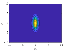
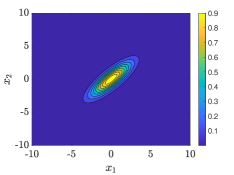
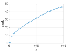
Figure 1: (a) Two-dimensional Gaussian stretched along the $x_{2}$-axis; (b) Two-dimensional rotated Gaussian (clockwise rotation by $\epsilon=\pi/4$ radians); (c) Rank of the the rotated Gaussian versus the clockwise rotation angle $\epsilon$.

Our contributions are as follows. First, we introduce a new class of functions that we refer to as ridge tensors, and provide a new method for evaluating $v(\bm{x})$ without losing the tensor compression of $u(\bm{x})$. Second, we develop a new Riemannian optimization algorithm for determining a linear map $\bm{A}$ so that $v(\bm{x})$ has smaller tensor rank than $u(\bm{x})$. Our approach is to parameterize the transformation $\bm{A}$ with a parameter $\epsilon\geq 0$, i.e., set $\bm{A}=\bm{A}(\epsilon)$, and consider $\bm{A}(\epsilon)$ as the flow map of an appropriate linear dynamical system. From this dynamical system perspective we derive a partial differential equation (PDE) for the $\epsilon$-dependent function $v(\bm{x};\epsilon)=u(\bm{A}(\epsilon)\bm{x})$. We then integrate the PDE for $v(\bm{x};\epsilon)$ using a step-truncation tensor integration scheme [36, 38, 23] to obtain $v(\bm{x};\epsilon)$ in a low-rank tensor format for all $\epsilon$. The quasi-optimal rank-reducing coordinate map $\bm{A}$ is obtained by minimizing a rank-related cost function using an appropriate path of transformations $\bm{A}(\epsilon)$. We construct such a path by giving the collection of linear transformations $\bm{A}(\epsilon)$ a Riemannian manifold structure and performing Riemannian gradient descent optimization, i.e., assigning to the derivative of the path $d\bm{A}(\epsilon)/d\epsilon$ a descent direction for the cost at each $\epsilon$ with respect to the chosen geometry. Our theoretical contributions provide a new framework that be generalized to larger classes of nonlinear transformations, and open new pathways for tensor rank reduction that are complementary to classical rank reduction methods, e.g., based on hierarchical SVD [15, 16]. Building upon our recent work on rank-adaptive tensor integrators [11], we also apply the new rank-reduction algorithm based on coordinate flows to linear PDEs. Specifically, we study advection problems in dimensions two, three and five and a reaction-diffusion equation in dimension two.

This paper is organized as follows. In section 2 we briefly review the functional tensor train (FTT) expansion, which, will be the main tensor format for demonstrating the proposed rank-reduction method based on coordinate flows. In section 3 we introduce ridge tensor trains and provide a simple example to illustrate the effects of coordinate flows on tensor rank. In section 4 we formulate the tensor rank reduction problem as a Riemannian optimization problem on the manifold of volume-preserving invertible coordinate maps. We also provide an efficient algorithm for computing the numerical solution to such optimization problem. In section 5 we demonstrate the proposed Riemannian gradient descent algorithm for computing quasi-optimal linear coordinate maps on a three-dimensional prototype function. In section 6 we apply the proposed rank reduction methods to PDEs in dimensions two, three and five and a reaction-diffusion equation in dimension two. We also include two appendices in which we describe the Riemannian manifold of coordinate flows, and provide theoretical results supporting the proposed mathematical framework for ridge tensors.

2 Functional tensor train (FTT) expansion

The coordinate flow rank reduction technique we propose in this paper can be applied to any tensor format, in particular to the functional tensor train (FTT) format [33, 6, 13]. In this section we briefly review the construction of FTT expansions for multivariate function belonging to the weighted Hilbert space

$$H=L^{2}_{\mu}(\Omega).$$ (3)

Here, $\Omega\subseteq\mathbb{R}^{d}$ is a separable domain such as a $d$-dimensional flat torus $\mathbb{T}^{d}$ or a Cartesian product of $d$ subsets of the real line

$$\Omega =\bigtimes_{i=1}^{d}\Omega_{i},\qquad\Omega_{i}\subseteq\mathbb{R},$$ (4)

and $\mu$ is a finite product measure on $\Omega$

$$\mu(\bm{x})=\prod_{i=1}^{d}\mu_{i}(x_{i}).$$ (5)

As is well-known (e.g., [33, 6, 13]), each element $u\in L^{2}_{\mu}(\Omega)$ admits a FTT expansion of the form

$$u(\bm{x})=\sum_{\alpha_{1},\ldots,\alpha_{d-1}=1}^{\infty}\sqrt{\lambda(\alpha_{d-1})}\psi_{1}(1;x_{1};\alpha_{1})\psi_{2}(\alpha_{1};x_{2};\alpha_{2})\cdots\psi_{d}(\alpha_{d-1};x_{d};1),$$ (6)

where $\{\psi_{i}(\alpha_{i-1};x_{i};\alpha_{i})\}_{\alpha_{i}}$ are orthonormal eigenfunctions of a hierarchy of compact self-adjoint operators. Orthonormality of $\{\psi_{i}(\alpha_{i-1};x_{i};\alpha_{i})\}_{\alpha_{i}}$ is relative to the inner products

$$\sum_{\alpha_{i-1}=1}^{\infty}\int_{\Omega_{i}}\psi_{i}(\alpha_{i-1};x_{i};\alpha_{i})\psi_{i}(\alpha_{i-1};x_{i};\beta_{i})d\mu_{i}(x_{i}) =\delta_{\alpha_{i}\beta_{i}},\qquad i=1,\ldots,d-1,\qquad\alpha_{0}=1,$$ (7)

$$\int_{\Omega_{d}}\psi_{d}(\alpha_{d-1};x_{d};1)\psi_{d}(\beta_{d-1};x_{d};1)d\mu_{d}(x_{d}) =\delta_{\alpha_{d-1}\beta_{d-1}}.$$

The sequence of positive real numbers $\left\{\sqrt{\lambda(\alpha_{d-1})}\right\}_{\alpha_{d-1}=1}^{\infty}$ appearing in (6) represents the product of all spectra of the compact self-adjoint operators mentioned above, and it has a single accumulation point at zero. By truncating such spectra so that only the largest eigenvalues and corresponding eigenfunctions are retained, we obtain the following FTT approximation of $u(\bm{x})$

$$u_{\text{\tiny TT}}(\bm{x})=\sum_{\alpha_{0}=1}^{r_{0}}\sum_{\alpha_{1}=1}^{r_{1}}\cdots\sum_{\alpha_{d}=1}^{r_{d}}\sqrt{\lambda(\alpha_{d-1})}\psi_{1}(\alpha_{0};x_{1};\alpha_{1})\psi_{2}(\alpha_{1};x_{2};\alpha_{2})\cdots\psi_{d}(\alpha_{d-1};x_{d};\alpha_{d}),$$ (8)

where $\bm{r}=(r_{0},r_{1},\ldots,r_{d-1},r_{d})$ is the tensor rank, $r_{0}=1$ and $r_{d}=1$. At this point it is convenient to define the following matrix-valued functions $\bm{\Psi}_{i}(x_{i})$ (known as tensor cores)

$$\bm{\Psi}_{1}(x_{1})= \begin{bmatrix}\psi_{1}(1;x_{1};1)&\cdots&\psi_{1}(1;x_{1};r_{1})\end{bmatrix},$$

$$\bm{\Psi}_{i}(x_{i})= \begin{bmatrix}\psi_{i}(1;x_{i};1)&\cdots&\psi_{i}(1;x_{i};r_{i})\\ \vdots&\ddots&\vdots\\ \psi_{i}(r_{i-1};x_{i};1)&\cdots&\psi_{i}(r_{r-1};x_{i};r_{i})\end{bmatrix}\qquad i=2,\ldots,d-1,$$

$$\bm{\Psi}_{d}(x_{d})= \begin{bmatrix}\psi_{d}(1;x_{d};1)\\ \vdots\\ \psi_{1}(r_{d-1};x_{d};1)\end{bmatrix},$$

and write (8) in a compact matrix product form

$$u_{\text{\tiny TT}}(\bm{x})=\bm{\Psi}_{1}(x_{1})\bm{\Psi}_{2}(x_{2})\cdots\sqrt{\bm{\Lambda}}\bm{\Psi}_{d}(x_{d}),$$ (9)

where $\bm{\Lambda}$ is a diagonal matrix with entries $\lambda(\alpha_{d-1})$ ($\alpha_{d-1}=1,\ldots,r_{d-1}$). To simplify notation further, we will often suppress explicit tensor core dependence on the spatial variable $x_{i}$, allowing us to write $\bm{\Psi}_{i}=\bm{\Psi}_{i}(x_{i})$ and $\psi_{i}(\alpha_{i-1},\alpha_{i})=\psi_{i}(\alpha_{i-1};x_{i};\alpha_{i})$ as the spatial dependence is indicated by the tensor core subscript “$i$”.

3 Tensor ridge functions

Let us introduce a new class of functions, which we call tensor ridge functions, that will be used in subsequent sections to build a tensor rank-reduction theory via linear coordinate mappings. To this end, consider the following invertible linear coordinate transformation

$$\bm{y}=\bm{A}\bm{x},\qquad\bm{A}:\mathbb{R}^{d}\to\mathbb{R}^{d}.$$ (10)

If we evaluate a function $u\in L^{2}_{\mu}(\Omega)$ at $\bm{y}$, we obtain the generalized ridge function $u(\bm{A}\bm{x})$ (e.g., [34]). Although the coordinate transformation $\bm{A}$ is linear, the evaluation of $u$ on $\bm{A}\bm{x}$ defines a nonlinear map of functions

$$u(\bm{x}) \mapsto v(\bm{x})=u(\bm{A}\bm{x}).$$ (11)

The image of a FTT tensor (8) under such a map has the form

$$u_{\text{\tiny TT}}(\bm{A}\bm{x})=\sum_{\alpha_{0}=1}^{r_{0}}\sum_{\alpha_{1}=1}^{r_{1}}\cdots\sum_{\alpha_{d}=1}^{r_{d}}\sqrt{\lambda(\alpha_{d-1})}\psi_{1}(\alpha_{0};\bm{a}_{1}\cdot\bm{x};\alpha_{1})\psi_{2}(\alpha_{1};\bm{a}_{2}\cdot\bm{x};\alpha_{2})\cdots\psi_{d}(\alpha_{d-1};\bm{a}_{d}\cdot\bm{x};\alpha_{d}),$$ (12)

which we call a tensor ridge function. In (12), $\bm{a}_{i}$ denotes the $i$-th row of the matrix $\bm{A}$ and “$\cdot$” is the standard dot product on $\mathbb{R}^{d}$, and $r_{0}=r_{d}=1$. When we consider $u_{\text{\tiny TT}}(\bm{A}\bm{x})=u_{\text{\tiny TT}}(\bm{y})$ in coordinates $\bm{y}$, equation (12) is the FTT expansion for $u_{\text{\tiny TT}}(\bm{y})$. However, when we consider $v(\bm{x})=u_{\text{\tiny TT}}(\bm{A}\bm{x})$ in coordinates $\bm{x}$ we have that each mode $\psi_{i}(\alpha_{i-1};\bm{a}_{i}\cdot\bm{x};\alpha_{i})$ in the tensor ridge function (12) is no longer a univariate function of $x_{i}$ as in (8), but rather a $d$-variate ridge function, which, has the property of being constant in all directions orthogonal to the vector $\bm{a}_{i}$ (e.g., [9, 34]). An important problem is determining the FTT expansion

$$v_{\text{\tiny TT}}(\bm{x})=\sum_{\alpha_{0}=1}^{s_{0}}\sum_{\alpha_{1}=1}^{s_{1}}\cdots\sum_{\alpha_{d}=1}^{s_{d}}\sqrt{\theta(\alpha_{d-1})}\varphi_{1}(\alpha_{0};x_{1};\alpha_{1})\varphi_{2}(\alpha_{1};x_{2};\alpha_{2})\cdots\varphi_{d}(\alpha_{d-1};x_{d};\alpha_{d})$$ (13)

given the FTT expansion (12) for $u_{\text{\tiny TT}}(\bm{A}\bm{x})$. A naive approach to solve this problem would be to recompute the FTT expansion from scratch using the methods of section 2, i.e., treat $v_{\text{\tiny TT}}(\bm{x})$ as a multivariate function and solve a sequence of hierarchical eigenvalue problems. This is not practical even for a moderate number of dimensions $d$ since the evaluation of $v(\bm{x})$ requires constructing a tensor product grid in $d$-dimensions, and each eigenvalue problem requires the computation of $d$-dimensional integrals. Another approach is to use TT-cross approximation [32], which provides an algorithm for interpolating $d$-dimensional black-box tensors in the tensor train format with computationally complexity that scales linearly with the dimension $d$. Hereafter, we develop a new approach to compute the FTT expansion (13) from (12) based on coordinate flows.

3.1 Computing tensor ridge functions via coordinate flows

Consider the non-autonomous linear dynamical system

$$\begin{cases}\displaystyle\frac{d\bm{y}(\epsilon)}{d\epsilon}=\bm{B}(\epsilon)\bm{y}(\epsilon),\\ \bm{y}(0)=\bm{x},\end{cases}$$ (14)

where $\bm{y}(\epsilon)\in\mathbb{R}^{d}$, and $\bm{B}(\epsilon)$ is a given $d\times d$ matrix with real entries for all $\epsilon\geq 0$. It is well-known that the solution to (14) can be written as

$$\bm{y}(\epsilon)=\bm{\Phi}(\epsilon)\bm{x},$$ (15)

where

$$\bm{\Phi}(\epsilon)=e^{\bm{M}(\epsilon)}$$ (16)

is an invertible linear mapping on $\mathbb{R}^{d}$ for each $\epsilon\geq 0$. The matrix $\bm{M}(\epsilon)$ can be represented by the Magnus series (e.g., [7])

$$\bm{M}(\epsilon)=\int_{0}^{\epsilon}\bm{B}(\epsilon_{1})d\bm{\epsilon}_{1}-\frac{1}{2}\int_{0}^{\epsilon}\left\{\int_{0}^{\epsilon_{1}}\bm{B}(\epsilon_{2})d\epsilon_{2},\bm{B}(\epsilon_{1})\right\}d\epsilon_{1}+\cdots,$$ (17)

where $\{\cdot,\cdot\}$ denotes the matrix commutator

$$\{\bm{P},\bm{Q}\}=\bm{P}\bm{Q}-\bm{Q}\bm{P}.$$ (18)

Now that we have introduced coordinate flows and their connection to linear coordinate transformations, let us consider the problem of determining the FTT expansion of $u_{\text{\tiny TT}}(\bm{A}\bm{x})$ when $\bm{A}$ is generated by a coordinate flow, i.e., $\bm{A}=\bm{\Phi}(\epsilon)$ for some $\bm{\Phi}$ and some $\epsilon\geq 0$. Differentiating $v(\bm{x};\epsilon)=u_{\text{\tiny TT}}(\bm{\Phi}(\epsilon)\bm{x})$ with respect to $\epsilon$ yields the hyperbolic PDE

$$\frac{\partial v(\bm{x};\epsilon)}{\partial\epsilon} =\frac{\partial u_{\text{\tiny TT}}(\bm{\Phi}(\epsilon)\bm{x})}{\partial\epsilon}$$ (19)

$$=\nabla u_{\text{\tiny TT}}(\bm{\Phi}(\epsilon)\bm{x})\cdot\left(\frac{\partial\bm{\Phi}(\epsilon)}{\partial\epsilon}\bm{x}\right)$$

$$=\nabla u_{\text{\tiny TT}}(\bm{\Phi}(\epsilon)\bm{x})\cdot\left(\bm{B}(\epsilon)\bm{\Phi}(\epsilon)\bm{x}\right),$$

where in the second line we used the chain rule and in the third line we used equations (14) and (15). Recalling $\bm{\Phi}(0)=\bm{I}_{d\times d}$ (identity matrix), we see that the initial state $v(\bm{x};0)=u_{\text{\tiny TT}}(\bm{x})$ is in FTT format. Thus, we have derived the following hyperbolic initial value problem for the tensor ridge function $v(\bm{x};\epsilon)$

$$\begin{cases}\displaystyle\frac{\partial v(\bm{x};\epsilon)}{\partial\epsilon}=\nabla v(\bm{x};\epsilon)\cdot\left(\bm{B}(\epsilon)\bm{\Phi}(\epsilon)\bm{x}\right),\\ v(\bm{x};0)=u_{\text{\tiny TT}}(\bm{x}),\end{cases}$$ (20)

with an initial condition that is given in an FTT format.

Integrating the PDE (20) forward in $\epsilon$ on a FTT tensor manifold, e.g. using rank-adaptive step-truncation methods [37, 36, 23] or dynamic tensor approximation methods [13, 12, 11, 28, 24], results in a FTT approximation $v_{\text{\tiny TT}}(\bm{x};\epsilon)$ of the function $v(\bm{x};\epsilon)$ for all $\epsilon\geq 0$. The computational cost of this approach for computing the FTT expansion of a FTT-ridge function is precisely the same cost as solving the hyperbolic PDE (20) in the FTT format, which in the case of step-truncation or dynamic approximation has computational complexity that scales linearly with $d$. Note that the accuracy of $v_{\text{\tiny TT}}(\bm{x};\epsilon)$ as an approximation of $v(\bm{x};\epsilon)$ depends on the $\epsilon$ step-size and order of integration scheme used to solve the PDE (20).

Using coordinate flows, it is straightforward to compute the FTT expansion of a tensor ridge function $u_{\text{\tiny TT}}(\bm{A}\bm{x})$ when the matrix $\bm{A}$ admits a real matrix logarithm $\bm{L}$. In this case, setting $\bm{B}(\epsilon)=\bm{L}$ yields $\bm{\Phi}(\epsilon)=e^{\epsilon\bm{L}}$, and therefore $\bm{A}=\bm{\Phi}(1)$. This means that we need to integrate (20) with $\bm{B}(\epsilon)=\bm{L}$ up to $\epsilon=1$ to obtain the FTT approximation of the tensor ridge function $u_{\text{\tiny TT}}(\bm{A}\bm{x})$. Let us provide a simple example.

An example

Consider the two-dimensional Gaussian function depicted in Figure 1(a), i.e.,

$$u_{\text{\tiny TT}}(\bm{x})=e^{-x_{1}^{2}-x_{2}^{2}/10}.$$ (21)

Clearly, (21) is the product of two univariate functions and therefore the FTT tensor representation coincides with (21) and has rank equal to one. Next, consider a simple linear coordinate transformation $\bm{\Phi}(\epsilon)$ which rotates the $(x_{1},x_{2})$-plane by an angle of $\epsilon$ radians. It is well-known that

$$\bm{\Phi}(\epsilon)=e^{\epsilon\bm{L}},$$ (22)

where

$$\bm{L}=\begin{bmatrix}0&-1\\ 1&0\end{bmatrix}$$ (23)

is the infinitesimal generator of the two-dimensional rotation. The dynamical system (14) defining the coordinate flow $\bm{y}(\epsilon)=\bm{\Phi}(\epsilon)\bm{x}$ can be written as

$$\begin{cases}\displaystyle\frac{d\bm{y}(\epsilon)}{d\epsilon}=\begin{bmatrix}0&-1\\ 1&0\end{bmatrix}\bm{y}(\epsilon),\\ \bm{y}(0)=\bm{x}.\end{cases}$$ (24)

The tensor ridge function corresponding to the coordinate map $\bm{\Phi}(\epsilon)$ is given analytically by

$$v(\bm{x};\epsilon) =u_{\text{\tiny TT}}(\bm{\Phi}(\epsilon)\bm{x})$$ (25)

$$=e^{-(\Phi_{11}(\epsilon)x_{1}+\Phi_{12}(\epsilon)x_{2})^{2}}e^{-(\Phi_{21}(\epsilon)x_{1}+\Phi_{22}(\epsilon)x_{2})^{2}/10}.$$

The hyperbolic PDE (20) for $v(\bm{x};\epsilon)$ in this case is given by

$$\begin{cases}\displaystyle\frac{\partial v(\bm{x};\epsilon)}{\partial\epsilon}=-x_{2}\displaystyle\frac{\partial v(\bm{x};\epsilon)}{\partial x_{1}}+x_{1}\displaystyle\frac{\partial v(\bm{x};\epsilon)}{\partial x_{2}},\\ v(\bm{x};0)=u_{\text{\tiny TT}}(\bm{x}).\end{cases}$$ (26)

It is straightforward to verify that (25) satisfies (26). Note that $v(\bm{x};\epsilon)$ in (25) is not an FTT tensor if $\epsilon\neq\pi k/2$ and $k\in\mathbb{N}$. To compute the FTT representation of $v_{\text{\tiny TT}}(\bm{x};\epsilon)$ we can solve the PDE (26) on a tensor manifold using step-truncation or dynamic tensor approximation methods [11, 13, 36, 38]. Given the low dimensionality of the spatial domain in this example ($d=2$), we can also evaluate (25) directly, and compute its FTT decomposition by solving an eigenvalue problem. In Figure 1 (b) we provide a contour plot of $v(\bm{x};\pi/4)$. To demonstrate the effect of rotations on tensor rank, in Figure 1(c) we plot the rank of $v(\bm{x};\epsilon)$ versus $\epsilon$ for all $\epsilon\in[0,\pi/4]$. Of course such a plot can be mirrored to obtain the rank for $\epsilon\in[\pi/4,\pi/2]$, $[\pi/2,3\pi/4]$, and $[3\pi/4,\pi]$.

4 Tensor rank reduction via coordinate flows

The coordinate flows we introduced in the previous section can be used to morph a given function into another one that has a faster decay rate of FTT singular values, i.e., a FTT tensor with lower rank (after truncation). A simple example is the coordinate flow that rotates the Gaussian function in Figure 1(b) back to the rank-one state depicted in Figure 1(a). This example and the examples documented in subsequent sections indicate that symmetry of the function relative to the new coordinate system plays an important role in reducing the tensor rank.

The problem of tensor rank reduction via linear coordinate flows can be formulated as follows: how do we choose an invertible linear coordinate transformation $\bm{A}$ so that $v_{\text{\tiny TT}}(\bm{x})\approx u_{\text{\tiny TT}}(\bm{A}\bm{x})$ has smaller rank than $u_{\text{\tiny TT}}(\bm{x})$ (eventually minimum rank)? The mathematical statement of this optimization problem is

$$\bm{A}=\operatorname*{\arg\!\min}_{\bm{A}\in{\rm GL}_{d}(\mathbb{R})}{\rm rank}\left[v_{\text{\tiny TT}}(\bm{x})\right],$$ (27)

where ${\rm GL}_{d}(\mathbb{R})$ denotes the set of $d\times d$ real invertible matrices, ${\rm rank}[\cdot]$ is a metric related to the FTT rank, and $v_{\text{\tiny TT}}(\bm{x})$ is a FTT approximation of $u_{\text{\tiny TT}}(\bm{A}\bm{x})$. In equation (27) we have purposely left the cost function unspecified, as some care must be taken in its definition to ensure that the optimization problem is both feasible and computationally effective in reducing rank. One possibility is to define ${\rm rank}[v_{\text{\tiny TT}}(\bm{x})]$ to return the sum of all $d$ entries of the multilinear rank vector $\bm{r}$ corresponding to the FTT tensor $v_{\text{\tiny TT}}(\bm{x})$. While such a cost function is effective in measuring tensor rank it yields a NP-hard rank optimization problem [27].

4.1 Non-convex relaxation for the rank minimization problem

A common relaxation for rank minimization problems is to replace the rank cost function with the sum of the singular values. To describe this relaxation in the context of FTT tensors we first recall that any FTT tensor $u_{\text{\tiny TT}}(\bm{x})$ can be orthogonalized in the $i$-th variable as (e.g., [11])

$$u_{\text{\tiny TT}}(\bm{x})=\bm{Q}_{\leq i}\bm{\Sigma}_{i}\bm{Q}_{>i},$$ (28)

where

$$\bm{\Sigma}_{i}={\rm diag}(\sigma_{i}(1),\sigma_{i}(2),\ldots,\sigma_{i}(r_{i})),$$ (29)

is a diagonal matrix with real entries (singular values of $u_{\text{\tiny TT}}$). The matrices $\bm{Q}_{\leq i}$ and $\bm{Q}_{>i}$ are defined as partial products

$$\bm{Q}_{\leq i}=\bm{Q}_{1}\bm{Q}_{2}\cdots\bm{Q}_{i},\quad\quad\bm{Q}_{>i}=\bm{Q}_{i+1}\bm{Q}_{i+2}\cdots\bm{Q}_{d},$$ (30)

and they satisfy the orthogonality conditions

$$\left\langle\bm{Q}_{\leq i}^{\text{T}}\bm{Q}_{\leq i}\right\rangle_{\leq i}=\bm{I}_{r_{i}\times r_{i}},\qquad\left\langle\bm{Q}_{>i}\bm{Q}_{>i}^{\text{T}}\right\rangle_{>i}=\bm{I}_{r_{i}\times r_{i}}.$$ (31)

Here, $\langle\cdot\rangle_{\leq i}$ and $\langle\cdot\rangle_{>i}$ are the averaging operators

$$\left\langle\bm{W}\right\rangle_{\leq i}(j,k)=\int_{\Omega_{\leq i}}w(j;\bm{x};k)d\mu_{\leq i}(\bm{x}_{\leq i}),\qquad\left\langle\bm{W}\right\rangle_{>i}(j,k)=\int_{\Omega_{>i}}w(j;\bm{x};k)d\mu_{>i}(\bm{x}_{>i}),$$ (32)

which map an arbitrary $r_{i}\times r_{i}$ matrix-valued function $\bm{W}(\bm{x})$ with entries $w(j;\bm{x};k)$ into another $r_{i}\times r_{i}$ matrix-valued function depending on a smaller number of variables. Using the orthogonalization (28) for each $i=1,2,\ldots,d-1$, we define the functions

$$S_{i}:L^{2}_{\mu}(\Omega) \to\mathbb{R}$$ (33)

$$u_{\text{\tiny TT}}(\bm{x}) \mapsto\sum_{\alpha_{i}=1}^{r_{i}}\sigma_{i}(\alpha_{i}),$$

which returns the sum of the singular values corresponding to the $i$-th component of the multilinear rank vector. Using these functions we define

$$S:L^{2}_{\mu}(\Omega) \to\mathbb{R}$$ (34)

$$u_{\text{\tiny TT}}(\bm{x}) \mapsto\sum_{i=1}^{d-1}\sum_{\alpha_{i}=1}^{r_{i}}\sigma_{i}(\alpha_{i}),$$

which is a relaxation of the rank cost function appearing in (27). An analogous relaxation of the rank cost function called the matrix nuclear norm has been studied extensively for matrix rank minimization problems [35, 27]. The function (34) has also been used as a relaxation of ${\rm rank}[\cdot]$ in tensor completion [5]. Next, we proceed by selecting an appropriate search space for the rank cost function. The largest search space we may choose is ${\rm GL}_{d}(\mathbb{R})$ as we have done in (27). This, however, is not a good choice since transformations in ${\rm GL}_{d}(\mathbb{R})$ are not volume-preserving and hence do not preserve $L^{2}$ norm, i.e., $\|u_{\text{\tiny TT}}(\bm{A}\bm{x})\|_{L^{2}_{\mu}}\neq\|u_{\text{\tiny TT}}(\bm{x})\|_{L^{2}_{\mu}}$. Transformations which do not preserve the norm of $u_{\text{\tiny TT}}(\bm{x})$ can reduce the rank cost function while having no impact on the tensor rank relative to the tensor’s norm. Therefore we choose ${\rm SL}_{d}(\mathbb{R})\subset{\rm GL}_{d}(\mathbb{R})$ as the search space, i.e., the collection of invertible matrices with determinant equal to one. These transformations are obviously volume-preserving, and therefore they preserve the $L^{2}$ norm of $u_{\text{\tiny TT}}$.

Since the domain of $S$ in (34) is $L^{2}_{\mu}(\Omega)$ and the cost function must be defined on the search space ${\rm SL}_{d}(\mathbb{R})$, we define an evaluation map $E$ corresponding to $u_{\text{\tiny TT}}(\bm{x})$

$$E:{\rm SL}_{d}(\mathbb{R}) \to L^{2}_{\mu}(\Omega)$$ (36)

$$\bm{A} \mapsto u_{\text{\tiny TT}}(\bm{A}\bm{x}).$$

Composing $E$ with $S$ yields the following (non-convex) relaxation of the cost function ${\rm rank}[\cdot]$ in (27)

$$C=S\circ E:{\rm SL}_{d}(\mathbb{R})\to\mathbb{R}.$$ (37)

The function $C(\bm{A})$ returns the sum of the singular values of the tensor ridge function $u_{\text{\tiny TT}}(\bm{A}\bm{x})$, where $\bm{A}$ is an invertible matrix with determinant equal to one. The optimization problem corresponding to the cost function and search space discussed above is

$$\bm{A}=\operatorname*{\arg\!\min}_{\bm{A}\in{\rm SL}_{d}(\mathbb{R})}C(\bm{A}).$$ (38)

While (38) is simpler than (27), it is still a computationally challenging problem for a number of reasons: First, it is non-convex. Second, when considered as a subset of all $d\times d$ matrices, the search space ${\rm SL}_{d}(\mathbb{R})$ is subject to a non-trivial set of constraints, e.g., $\det(\bm{A})=1$. Third, we note that the set ${\rm SL}_{d}(\mathbb{R})$ is unbounded (matrices with determinant $1$ can have entries that are arbitrarily large). This can yield convergence issues when looking for the minimizer (38). In order to overcome this problem one may introduce linear inequality constraints on the entries of the matrix $\bm{A}$, i.e., optimize over bounded subsets of ${\rm SL}_{d}(\mathbb{R})$ such as the set of rotation matrices with determinant $1$.

Hereafter we develop a new method for obtaining a local minimum of (38). To handle the search space constraints, we give ${\rm SL}_{d}(\mathbb{R})$ a Riemannian manifold structure and perform gradient descent on this manifold [1]. To obtain the gradient of $C(\bm{A})$ efficiently we build its computation into the FTT truncation procedure at a negligible additional computational cost.

4.2 Riemannian gradient descent path

In Lemma B4 we show that if the FTT singular values of $u_{\text{\tiny TT}}(\bm{A}\bm{x})$ are simple (i.e., distinct) then the cost function $C(\bm{A})$ defined in (37) is differentiable in $\bm{A}$. With this sufficient condition for the smoothness of the cost function established, we can use the machinery of Riemannian geometry summarized in A to construct a gradient descent path for the minimization of (38) on the search space ${\rm SL}_{d}(\mathbb{R})$. To this end, let us denote by $\bm{\Gamma}(\epsilon)$ such gradient descent path. To build $\bm{\Gamma}(\epsilon)$, we start at the identity $\bm{\Gamma}(0)=\bm{I}$ and consider the matrix ordinary differential equation

$$\begin{cases}\displaystyle\frac{d\bm{\Gamma}(\epsilon)}{d\epsilon}=-{\rm grad}\left[C\left(\bm{\Gamma}\left(\epsilon\right)\right)\right],\\ \bm{\Gamma}(0)=\bm{I},\end{cases}$$ (39)

where ${\rm grad}\left[C\left(\bm{\Gamma}\left(\epsilon\right)\right)\right]$ is the Riemannian gradient of the cost function $C$ defined in (37). By construction, the vector $-{\rm grad}\left[C(\bm{\Gamma}(\epsilon))\right]$ is tangent to the manifold ${\rm SL}_{d}(\mathbb{R})$ at each point $\bm{\Gamma}\left(\epsilon\right)$, and thus $\bm{\Gamma}(\epsilon)\in{\rm SL}_{d}(\mathbb{R})$ for all $\epsilon\geq 0$. Since $-{\rm grad}\left[C\left(\bm{\Gamma}\left(\epsilon\right)\right)\right]$ points in the direction of steepest descent of the cost function $C$ at the point $\bm{\Gamma}(\epsilon)$, the cost function is guaranteed to decrease along the path $\bm{\Gamma}(\epsilon)$ (or remain constant which implies we have obtained a local minimum). In Figure 2 we provide an illustration of the Riemannian gradient descent path $\bm{\Gamma}(\epsilon)$. For computational efficiency, it is essential to have a fast method for computing the Riemannian gradient of the cost function $C$ at an arbitrary point $\bm{A}\in{\rm SL}_{d}(\mathbb{R})$. The following Proposition provides an expression for such Riemannian gradient in terms of orthogonal FTT cores which we will use to efficiently compute the descent direction. The proof is given in B.

Proposition 4.1.

The Riemannian gradient of the cost function (37) at the point $\bm{A}\in{\rm SL}_{d}(\mathbb{R})$ is given by

$${\rm grad}\left[C\left(\bm{A}\right)\right]=\bm{D}\bm{A},$$ (40)

where

$${\bm{D}}=\sum_{i=1}^{d-1}\int_{\Omega}\bm{Q}_{\leq i}\bm{Q}_{>i}\left(\nabla v(\bm{x})\left(\bm{A}\bm{x}\right)^{\text{T}}-\frac{\nabla v(\bm{x})^{\text{T}}\bm{A}\bm{x}}{d}\bm{I}_{d\times d}\right)d\mu(\bm{x}),$$ (41)

$v(\bm{x})=u_{\text{\tiny TT}}(\bm{A}\bm{x})$ and $\bm{Q}_{\leq i},\bm{Q}_{>i}$ are tensor cores of the orthogonalized FTT

$$v(\bm{x})=\bm{Q}_{\leq i}\bm{\Sigma}_{i}\bm{Q}_{>i}.$$ (42)

  (a)                                                                          (b)

         

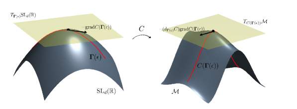
Figure 2: An illustration of a descent path $\bm{\Gamma}(\epsilon)$ for the cost function $C$ defined in (37). At each point of the path $\bm{\Gamma}(\epsilon)\in{\rm SL}_{d}(\mathbb{R})$ we assign the tangent vector $-{\rm grad}\left[C(\bm{\Gamma}(\epsilon))\right]\in T_{\bm{\Gamma}(\epsilon)}{\rm SL}_{d}(\mathbb{R})$ which points in the direction of steepest descent $-(d_{\bm{\Gamma}(\epsilon)}C){\rm grad}\left[C(\bm{\Gamma}(\epsilon))\right]\in T_{C(\bm{\Gamma}(\epsilon))}\mathcal{M}$ of the function $C$ at the point $C(\bm{\Gamma}(\epsilon))\in\mathcal{M}$.

Using the gradient descent path defined by (39) we differentiate the coordinate transformation

$$\bm{y}(\epsilon)=\bm{\Gamma}(\epsilon)\bm{x}$$ (43)

with respect to $\epsilon$ and use (39)-(40) to obtain

$$\begin{cases}\displaystyle\frac{d\bm{y}(\epsilon)}{d\epsilon}=-\bm{D}(\epsilon)\bm{y}(\epsilon),\\ \bm{y}(0)=\bm{x}.\end{cases}$$ (44)

Note that (44) has the same form as the ODE (14) we used to define coordinate flows. Hence, by construction, the flow map generated by (44) is the descent path $\bm{\Gamma}(\epsilon)$ on the manifold ${\rm SL}_{d}(\mathbb{R})$, which, converges to a local minimum of $C$ as $\epsilon$ increases. By defining the function $v(\bm{x};\epsilon)=u_{\text{\tiny TT}}(\bm{\Gamma}(\epsilon)\bm{x})$ and differentiating it with respect to $\epsilon$ we obtain the hyperbolic PDE

$$\begin{cases}\displaystyle\frac{\partial v(\bm{x};\epsilon)}{\partial\epsilon}=-\nabla v(\bm{x};\epsilon)\cdot\left[\bm{D}(\epsilon)\bm{\Gamma}(\epsilon)\bm{x}\right],\\ v(\bm{x};0)=u_{\text{\tiny TT}}(\bm{x}).\end{cases}$$ (45)

Note that the evolution of $\bm{y}(\epsilon)=\bm{\Gamma}(\epsilon)\bm{x}$ at the right hand side of (45) is defined by (44). Integrating (44)-(45) forward in $\epsilon$ yields a rank-reducing linear coordinate transformation $\bm{\Gamma}(\epsilon)$ and the reduced rank function $v(\bm{x};\epsilon)=u_{\text{\tiny TT}}\left(\bm{\Gamma}(\epsilon)\bm{x}\right)$.

4.3 Numerical integration of the gradient descent equations

It is convenient to use a step-truncation method [36, 38, 23] to integrate the initial value problem (45) on a FTT tensor manifold. This is because applying the FTT truncation operation to $v(\bm{x};\epsilon)$ requires computing the orthogonalized tensor cores $\bm{Q}_{\leq i}(\epsilon),\bm{Q}_{>i}(\epsilon)$ $(i=1,2,\ldots,d-1)$ which can then be readily used to evaluate the matrix $\bm{D}(\epsilon)$ defining the Riemannian gradient (41). Moreover, the FTT truncation operation applied to $v(\bm{x};\epsilon)$ yields an expansion of the form (13), which is the desired tensor format. To describe the integration algorithm in more detail, let us discretize the interval $[0,\epsilon_{f}]$ into $N+1$ evenly-spaced points

$$\epsilon_{i}=i\Delta\epsilon,\qquad\Delta\epsilon=\frac{\epsilon_{f}}{N},\qquad i=0,1,\ldots,N,$$ (46)

and let $v_{i},\bm{\Gamma}_{i},\bm{D}_{i}$ denote $v(\bm{x};\epsilon_{i}),\bm{\Gamma}(\epsilon_{i}),\bm{D}(\epsilon_{i})$, respectively. Let

$$v_{i+1} =v_{i}+\Delta\epsilon\Phi\left(v_{i},\bm{D}_{i},\Delta\epsilon\right),$$ (47)

$$\bm{\Gamma}_{i+1} =\bm{\Gamma}_{i}+\Delta\epsilon\widehat{\bm{\Phi}}\left(\bm{\Gamma}_{i},\bm{D}_{i},\Delta\epsilon\right)$$ (48)

be one-step explicit integration schemes approximating the solution to the initial value problem (45) and the matrix ODE (39), respectively. In order to guarantee that the solution $v_{i+1}$ is a low-rank FTT tensor, we apply a truncation operator to the right hand side of (47). This yields the step-truncation method [36]

$$v_{i+1}=\mathfrak{T}_{\delta}\left(v_{i}+\Delta\epsilon\Phi\left(v_{i},\bm{D}_{i},\Delta\epsilon\right)\right).$$ (49)

Here, $\mathfrak{T}_{\delta}$ denotes the standard FTT truncation operator with relative accuracy $\delta$ proposed in [33] modified to return the matrix $\bm{D}_{i+1}$. A detailed description of the modified tensor truncation algorithm is provided in section 4.4.

At this point, a few remarks regarding the integration scheme (47)-(49) are in order. First, we notice that at each step of the gradient descent algorithm we are computing the gradient (40) at the identity matrix since the current tensor $v_{i}$ is the tensor ridge function $v_{i}(\bm{x})=u_{\text{\tiny TT}}(\bm{\Gamma}_{i}\bm{x})$. Second, the accuracy of the tensor $v_{i}$ approximating $u_{\text{\tiny TT}}(\bm{\Gamma}_{i}\bm{x})$ is determined by the chosen integration scheme and its relevant parameters (i.e., the function $\Phi$, the step size $\Delta\epsilon$, and the accuracy of $\mathfrak{T}_{\delta}$). In a standard gradient descent algorithm, convergence can be expedited with a line-search routine that determines an appropriate step-size to take in the descent direction. However, in the proposed integration scheme the step-size determines the accuracy of the final tensor, thus we keep the step-size $\Delta\epsilon$ fixed during gradient descent. We set a stopping criterion for the integration of (47)-(49) based on the empirical observation that the cost function $C$ does not decrease substantially along the descent path $\bm{\Gamma}(\epsilon)$ when $\bm{\Gamma}_{i}$ is close to a local minimum. Mathematically, this translates into the condition

$$\frac{dS(v_{i})}{d\epsilon}>-{\eta},$$ (50)

where ${\eta}$ is some predetermined tolerance. Since the solution history $v_{i},v_{i-1},\ldots$ is available during gradient descent, a simple method for approximating $dS(v_{i})/d\epsilon$ is a $p$-point backwards difference stencil

$$\frac{dS(v_{i})}{d\epsilon}\approx{\rm BD}^{(p)}(S(v_{i}),{S(v_{i-1})},\ldots,S(v_{i-p})).$$ (51)

In addition to the stopping criterion (50), we also set a maximum number of iterations $M_{\rm iter}$ to ensure that the Riemannian gradient descent algorithm halts within a reasonable amount of time. We summarize the proposed Riemannian gradient descent method to compute a local minimum of (38) in Algorithm 1.

Input:

$u_{\text{\tiny TT}}$ $\rightarrow$ initial FTT tensor,

$\Delta\epsilon$ $\rightarrow$ step-size for gradient descent,

${\eta}$ $\rightarrow$ stopping tolerance,

$M_{\rm iter}$ $\rightarrow$ maximum number of iterations.

Output:

$\bm{\Gamma}$ $\rightarrow$ rank-reducing linear coordinate transformation,

$v_{\text{\tiny TT}}$ $\rightarrow$ reduced rank FTT tensor on transformed coordinates $v_{\text{\tiny TT}}(\bm{x})=u_{\text{\tiny TT}}(\bm{\Gamma}\bm{x})$ .

Runtime:

• $[v_{0},S(v_{0}),\bm{D}_{0}]=\mathfrak{T}_{\delta}(u_{\text{\tiny TT}})$,

$\bm{\Gamma}_{0}=\bm{I}$,

$\dot{S}(v_{0})=-\infty$,

$i=0$.

while $\dot{S}(v_{i})<-{\eta}$ and $i\leq M_{\rm iter}$

• $v_{i+1}=v_{i}+\Delta\epsilon\Phi(v_{i},\bm{D}_{i},\Delta\epsilon)$,

• $[v_{i+1},S(v_{i+1}),\bm{D}_{i+1}]=\mathfrak{T}_{\delta}(v_{i+1})$,

• $\bm{\Gamma}_{i+1}=\bm{\Gamma}_{i}+\Delta\epsilon\widehat{\bm{\Phi}}(\bm{\Gamma}_{i},\bm{D}_{i},\Delta\epsilon)$,

• $\dot{S}(v_{i+1})={\rm BD}^{(p)}(S(v_{i+1}),S(v_{i}),\ldots,S(v_{i+1-p}))$,

• $i=i+1$,

• $\bm{\Gamma}=\bm{\Gamma}_{i}$,

• $v_{\text{\tiny TT}}=v_{i}$.

end

Algorithm 1 Riemannian gradient descent for computing rank-reducing linear coordinate maps.

4.4 Modified tensor truncation algorithm

         

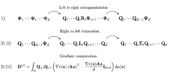
Figure 3: A summary of the modified FTT truncation algorithm for computing the Riemannian gradient (41).

Input:

$v$ $\rightarrow$ FTT tensor with cores $\bm{\Psi}_{1},\bm{\Psi}_{2},\ldots,\bm{\Psi}_{d}$,

$\delta$ $\rightarrow$ desired accuracy.

Output:

$v_{\text{\tiny TT}}$ $\rightarrow$ truncated FTT tensor satisfying $\|v-v_{\text{\tiny TT}}\|_{L^{2}_{\mu}(\Omega)}\leq\delta\|v\|_{L^{2}_{\mu}(\Omega)}$,

$S\left(v_{\text{\tiny TT}}\right)$ $\rightarrow$ sum of all multilinear singular values of $v_{\text{\tiny TT}}$,

$\bm{D}$ $\rightarrow$ left factor of the Riemannian gradient (40).

Runtime:

• $\hat{\delta}=\displaystyle\frac{\delta}{\sqrt{d-1}}\|v\|_{L^{2}}$          (Set truncation parameter)

• $S(v)=0$                       (Initialize $S(v)$)

• for $i=1$ to $d-1$           (Left-to-right orthogonalization)

  • $[\bm{Q}_{i},\bm{R}_{i}]={\rm QR}(\bm{\Psi}_{i})$

  • $\bm{\Psi}_{i+1}=\bm{R}_{i}\bm{\Psi}_{i+1}$

end

for $i=d$ to $2$           (Right-to-left truncation and gradient computation)

• $[\bm{L}_{i},\bm{Q}_{i}]={\rm LQ}(\bm{\Psi}_{i})$

• $[\bm{U}_{i},\bm{\Sigma}_{i},\bm{V}_{i}]={\rm SVD}_{\hat{\delta}}(\bm{L}_{i})$

• $\bm{Q}_{i}=\bm{V}_{i}^{\text{T}}\bm{Q}_{i}$

• $\bm{Q}_{i-1}=\bm{Q}_{i-1}\bm{U}_{i}$,

• $S(v)=S(v)+{\rm sum}\left(\Sigma_{i}\right)$,

• $\bm{D}^{(i-1)}=\int\bm{Q}_{\leq i-1}\bm{Q}_{>i-1}\left(\nabla v(\bm{x})\bm{x}^{\text{T}}\right)d\mu(\bm{x})$

end $\bm{D}=\displaystyle\sum_{i=1}^{d-1}\bm{D}^{(i)}$.

$v_{\text{\tiny TT}}=\bm{Q}_{1}\bm{\Sigma}_{2}\bm{Q}_{2}\ldots\bm{Q}_{d}$.

Algorithm 2 Modified FTT truncation algorithm.

To speed up numerical integration of the gradient descent equations (48)-(49) it is convenient to compute the matrix $\bm{D}_{i}$ defined in (41) during FTT truncation. The reason being that standard FTT truncation requires the computation of all orthogonal FTT cores $\bm{Q}_{\leq j}$ and $\bm{Q}_{>j}$, which, can be readily used to compute $\bm{D}_{i}$. To describe the modified tensor truncation algorithm, let $v_{\text{\tiny TT}}(\bm{x})=\bm{\Psi}_{1}\cdots\bm{\Psi}_{d}$ be an FTT tensor with non-optimized rank, e.g., $v_{\text{\tiny TT}}(\bm{x})$ is the result of adding two FTT tensors together. Denote by $\mathfrak{T}_{\delta}$ the modified truncation operator, where $\delta$ is the required relative accuracy, i.e.,

$$\|v_{\text{\tiny TT}}(\bm{x})-\mathfrak{T}_{\delta}(v_{\text{\tiny TT}}(\bm{x}))\|_{L^{2}_{\mu}(\Omega)}\leq\delta\|v_{\text{\tiny TT}}(\bm{x})\|_{L^{2}_{\mu}(\Omega)}.$$ (52)

We also define

$$\hat{\delta}=\frac{\delta}{\sqrt{d-1}}\|v_{\text{\tiny TT}}(\bm{x})\|_{L^{2}_{\mu}(\Omega)},$$ (53)

which is the required accuracy for each SVD in the FTT truncation algorithm. As described in [11], we may perform a functional analogue of the QR decomposition on the FTT tensor cores of $v_{\text{\tiny TT}}(\bm{x})$

$$\bm{\Psi}_{i}=\bm{Q}_{i}\bm{R}_{i},$$ (54)

where $\bm{Q}_{i}$ is a $r_{i-1}\times r_{i}$ matrix with elements in $L^{2}_{\mu_{i}}(\Omega_{i})$ satisfying $\left\langle\bm{Q}_{i}^{\text{T}}\bm{Q}_{i}\right\rangle_{i}=\bm{I}_{r_{i}\times r_{i}}$, and $\bm{R}_{i}$ is an upper triangular $r_{i}\times r_{i}$ matrix with real entries. Similarly, we can perform an LQ-factorization

$$\bm{\Psi}_{i}=\bm{L}_{i}\bm{Q}_{i},$$ (55)

where $\bm{Q}_{i}$ is a $r_{i-1}\times r_{i}$ matrix with elements in $L^{2}_{\mu_{i}}(\Omega_{i})$ satisfying $\left\langle\bm{Q}_{i}^{\text{T}}\bm{Q}_{i}\right\rangle_{i}=\bm{I}_{r_{i}\times r_{i}}$, and $\bm{L}_{i}$ is a lower-triangular $r_{i}\times r_{i}$ matrix with real entries. The first procedure in the modified truncation routine is a left-to-right orthogonalization sweep in which we first perform the QR decomposition

$$\bm{\Psi}_{1}=\bm{Q}_{1}\bm{R}_{1},$$ (56)

and then update the core $\bm{\Psi}_{2}$

$$\bm{\Psi}_{2}=\bm{R}_{1}\bm{\Psi}_{2}.$$ (57)

This process is repeated recursively

$$\bm{\Psi}_{i}=\bm{Q}_{i}\bm{R}_{i},\qquad\bm{\Psi}_{i+1}=\bm{R}_{i}\bm{\Psi}_{i+1},\qquad i=2,\ldots,d-1,$$ (58)

resulting in the orthogonalization

$$v_{\text{\tiny TT}}(\bm{x})=\bm{Q}_{1}\bm{Q}_{2}\cdots\bm{Q}_{d-1}\bm{\Psi}_{d}.$$ (59)

Next, we perform a right-to-left sweep which compresses $v_{\text{\tiny TT}}(\bm{x})$ and simultaneously computes each term appearing in the summation of $\bm{D}$ in equation (41). The first step of this procedure is to compute a LQ decomposition of $\bm{\Psi}_{d}$

$$\bm{\Psi}_{d}=\bm{L}_{d}\bm{Q}_{d},$$ (60)

and then perform a truncated singular value decomposition of $\bm{L}_{d}$ with threshold $\hat{\delta}$

$$\bm{L}_{d}=\bm{U}_{d}\bm{\Sigma}_{d}\bm{V}_{d}^{\text{T}}.$$ (61)

Substituting (60) and (61) into (59) yields

$$v_{\text{\tiny TT}}(\bm{x})=\bm{Q}_{1}\bm{Q}_{2}\cdots\bm{Q}_{d-1}\bm{\Sigma}_{d}\bm{Q}_{d},$$ (62)

where we re-defined

$$\bm{Q}_{d-1}=\bm{Q}_{d-1}\bm{U}_{d},\qquad\bm{Q}_{d}=\bm{V}_{d}^{\text{T}}\bm{Q}_{d}.$$ (63)

At this point we have truncated the FTT tensor $v_{\text{\tiny TT}}(\bm{x})$ in the $d$-th variable. The expansion (63) provides the FTT orthogonalization needed to compute the $(d-1)$-th term in the sum (41)

$$\bm{D}^{(d-1)}=\int_{\Omega}\bm{Q}_{\leq d-1}\bm{Q}_{>d}\left(\nabla v_{\text{\tiny TT}}(\bm{x})\bm{x}^{\text{T}}\right)d\mu(\bm{x}),$$ (64)

which, can be computed efficiently by applying one-dimensional differentiation matrices and quadrature rules to the FTT cores. We proceed in a recursive manner ($i=d-1,\ldots,2$) with the same steps described above for $\bm{\Psi}_{d}$. First compute the LQ decomposition

$$\left(\bm{Q}_{i}\bm{\Sigma}_{i+1}\right)=\bm{L}_{i}\bm{Q}_{i},$$ (65)

and then perform a singular value decomposition with threshold $\hat{\delta}$

$$\bm{L}_{i}=\bm{U}_{i}\bm{\Sigma}_{i}\bm{V}_{i}^{\text{T}}.$$ (66)

Then rewrite $v_{\text{\tiny TT}}(\bm{x})$ as

$$v_{\text{\tiny TT}}(\bm{x})=\bm{Q}_{1}\bm{Q}_{2}\cdots\bm{Q}_{i-1}\bm{\Sigma}_{i}\bm{Q}_{i}\cdots\bm{Q}_{d},$$ (67)

where we re-defined

$$\bm{Q}_{i-1}=\bm{Q}_{i-1}\bm{U}_{i},\qquad\bm{Q}_{i}=\bm{V}_{i}^{\text{T}}\bm{Q}_{i}.$$ (68)

The expansion (67) provides the FTT orthogonalization required to compute the $(i-1)$-th term in the sum (41)

$$\bm{D}^{(i-1)}=\int_{\Omega}\bm{Q}_{\leq i-1}\bm{Q}_{>i}\left(\nabla v_{\text{\tiny TT}}(\bm{x})\bm{x}^{\text{T}}\right)d\mu(\bm{x}),$$ (69)

which, can be computed efficiently by applying one-dimensional differentiation matrices and quadrature rules to the FTT cores. Finally with all of the terms in (41) computed we simply sum them to obtain the matrix

$$\bm{D}=\displaystyle\sum_{i=1}^{d-1}\bm{D}^{(i)}.$$ (70)

We summarize the main steps of the modified tensor truncation in Figure 3 and in Algorithm 2. Clearly, the matrix $\bm{D}$ needs to be recomputed at each step $\epsilon_{i}$, resulting in the matrix $\bm{D}_{i}$ appearing in the gradient descent equations (48)-(49).

4.5 Computational cost

One step of a first-order step-truncation integrator of the form (49) (e.g. Euler forward) without computing the left factor of the Riemannian gradient (41) requires one multiplication between a scalar and a TT tensor ($\mathcal{O}(nr^{2})$ FLOPS), one addition between two TT tensors, and one FTT truncation ($\mathcal{O}(dnr^{3})$ FLOPS) for a total computational complexity $\mathcal{O}(dnr^{3})$. In the above estimate we assumed that each entry of the rank of the FTT tensor $v_{i}+\Delta\epsilon\Phi(v_{i},\bm{D}_{i},\Delta\epsilon)$ is bounded by $r$ and $v_{i}$ is discretized on a grid with $n$ points in each variable. In addition to the cost of step-truncation, we must also compute the matrix $\bm{D}_{i}$ defined in (41) at each step. The orthogonal FTT cores $\bm{Q}_{\leq j},\bm{Q}_{>j}$ needed for the computation of $\bm{D}_{i}$ are readily available during the tensor truncation procedure. For the computation of $\bm{D}_{i}$ we must compute the gradient of $\nabla v_{i}$, which requires $d$ matrix multiplications between a differentiation matrix of size $n\times n$ and a FTT core $\bm{\Psi}_{i}$ of size $n\times rn$ for total complexity of $\mathcal{O}(dn^{3}r)$. We also need to compute the outer product $(\nabla v_{i})\bm{x}^{\text{T}}$ where each entry of $\nabla v_{i}$ is in FTT format, and, for each of the $d^{2}$ entries in the matrix $(\nabla v_{i})\bm{x}^{\text{T}}$ compute an integral of FTT tensors requiring $\mathcal{O}(dnr^{3})$ FLOPS. The final estimate for computing the matrix $\bm{D}_{i}$ is $\mathcal{O}(d^{2}n^{3}r^{3})$, which dominates the cost of performing one-step of (49). We point out that the computation of $\bm{D}_{i}$ may be incorporated into high performance computing algorithms for tensor train rounding, e.g., [2, 41].

5 Application to multivariate functions

We now demonstrate the Riemannian gradient descent algorithm for generating rank-reducing linear coordinate transformations. Consider the Gaussian mixture

$$u(\bm{x})=\sum_{i=1}^{N_{g}}w_{i}\exp\left(-\sum_{j=1}^{d}\frac{1}{\beta_{ij}}\left(\bm{R}^{(i)}_{j}\cdot\bm{x}+t_{ij}\right)^{2}\right),$$ (71)

where $N_{g}$ is the number of Gaussians, $\beta_{ij}$ are positive real numbers, $w_{i}$ are positive weights satisfying

$$\sum_{i=1}^{d}w_{i}=1,$$

$\bm{R}_{j}^{(i)}$ is the $j$-th row of a $d\times d$ rotation matrix $\bm{R}^{(i)}$, and $t_{ij}$ are translations.

       (a)                                                                             (b)

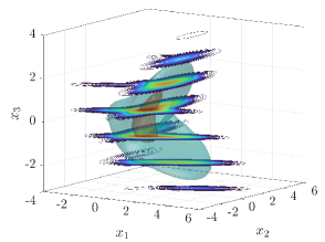
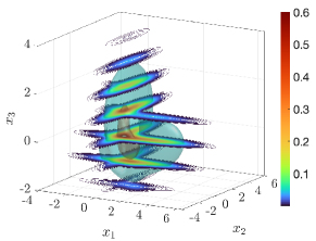
Figure 4: (a) Volumetric plot of the three-dimensional Gaussian mixture (71). (b) Volumetric plot of the corresponding reduced rank ridge tensor $v(\bm{x};\epsilon_{f})$.

       (a)                                                                                       (b)

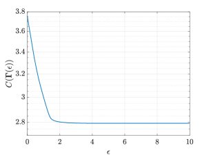
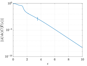
Figure 5: Rank reduction problem via coordinate flow for the three-dimensional Gaussian mixture (71). (a) Cost function (38) evaluated along a steepest descent mapping $\bm{\Gamma}(\epsilon)$ versus $\epsilon$. (b) Absolute value of the derivative of the cost function in (38) versus $\epsilon$. The derivative is computed with a second-order backwards finite difference stencil (51).

For our demonstration we consider three spatial dimensions ($d=3$) and set $N_{g}=3$, $w_{i}=1/3$,

$$\begin{array}[]{l l l}\beta_{11}=2,&\beta_{12}=1/3,&\beta_{13}=1/2,\\ \beta_{21}=3,&\beta_{22}=4,&\beta_{23}=1/6,\\ \beta_{31}=1,&\beta_{32}=1/5,&\beta_{33}=5,\end{array}\qquad\begin{array}[]{l l l}t_{11}=0,&t_{12}=0,&t_{13}=0,\\ t_{21}=-1,&t_{22}=1/2,&t_{23}=-1/3,\\ t_{31}=1/2,&t_{32}=-1/4,&t_{33}=1,\end{array}$$ (72)

and the rotation matrices

$$\bm{R}^{(i)}=\exp\left(\begin{bmatrix}0&\theta_{i}(1)&\theta_{i}(2)\\ -\theta_{i}(1)&0&\theta_{i}(3)\\ -\theta_{i}(2)&-\theta_{i}(3)&0\end{bmatrix}\right),$$ (73)

with

$$\bm{\theta}_{1}=\begin{bmatrix}\pi/4\\ \pi/3\\ \pi/5\end{bmatrix},\quad\bm{\theta}_{2}=\begin{bmatrix}\pi/3\\ \pi/6\\ \pi/4\end{bmatrix},\quad\bm{\theta}_{3}=\begin{bmatrix}\pi/3\\ \pi/3\\ \pi/7\end{bmatrix}.$$ (74)

We discretize the Gaussian mixture (71) on the computational domain $[-12,12]^{3}$ (which is large enough to enclose the numerical support of (71)) using $200$ evenly-spaced points in each variable. From the discretization of (71) we compute the FTT decomposition $u_{\text{\tiny TT}}(\bm{x})$ using recursive SVDs.

(a)                                                                               (b)

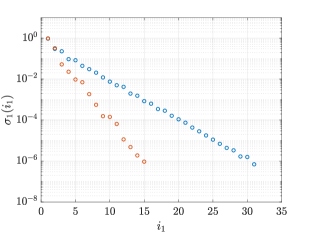
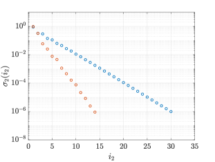
(c)

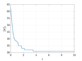
Figure 6: Multilinear spectra of the 3-dimensional Gaussian mixture $v(\bm{x};0)$ defined in (71) (Cartesian coordinates) and the corresponding reduced-rank ridge tensor $v(\bm{x};\epsilon_{f})$ (transformed coordinates). (a) Spectra $\sigma_{1}$ corresponding to multilinear rank $r_{1}$. (b) Spectra $\sigma_{2}$ corresponding to multilinear rank $r_{2}$. (c) $1$-norm of the multilinear rank vector of $v_{\text{\tiny TT}}(\bm{x};\epsilon)$ versus $\epsilon$. It is seen that the coordinate flow $\bm{\Gamma}(\epsilon)\bm{x}$ reduces the multilinear rank of the Gaussian mixture (71) from about $63$ (Cartesian coordinates) to $31$ (transformed coordinates).

To integrate the PDE (45) for the reduced rank ridge tensor $v(\bm{x};\epsilon)$, we use the explicit two-step Adams-Bashforth step-truncation method with $\Delta\epsilon=10^{-3}$ and relative FTT truncation accuracy $\delta=10^{-6}$. All spatial derivatives and integrals are computed by applying one-dimensional pseudo-spectral Fourier differentiation matrices and quadrature weights [18] to the tensor modes. We integrate up to $\epsilon_{f}=10$ which is sufficient to demonstrate convergence of the gradient descent method. In Figure 4 we provide volumetric plots of the of the function $v(\bm{x};\epsilon)$ for $\epsilon=0$ and $\epsilon=\epsilon_{f}$. We observe that the reduced rank ridge tensor $v(\bm{x};\epsilon_{f})$ appears to be more symmetrical with respect to the $(x_{1},x_{2},x_{3})$-axes than the higher rank function $v(\bm{x};0)$. In Figure 5(a) we plot the cost function $C(\bm{\Gamma}(\epsilon))$ versus $\epsilon$ and in Figure 5(b) we plot the absolute value of the derivative of the cost function versus $\epsilon$. Observe in Figure 5 that $\bm{\Gamma}(\epsilon)$ appears to be converging to a local minimum of $C$, and, the majority of the decrease in the cost function occurs in the interval $\epsilon\in[0,2]$. Correspondingly, we notice that in Figure (6)(c) the majority of rank increase occurs in the interval $\epsilon\in[0,2]$. Finally, in Figure 6(a)-(b) we plot the multilinear spectra of the function $v_{\text{\tiny TT}}(\bm{x};\epsilon)$ for $\epsilon=0$ and $\epsilon=\epsilon_{f}$. The decay rate of the multilinear spectra corresponding to $v(\bm{x};\epsilon_{f})$ is significantly faster than the decay rate of the multilinear corresponding to the initial function $v(\bm{x};0)$, resulting in a multilinear rank of about half the one in Cartesian coordinates. Thus, for any truncation tolerance $\delta$, the FTT-ridge tensor $v(\bm{x};\epsilon_{f})$ can be stored at a significantly lower cost than the original function. Intuitively, the savings that can be obtained by the coordinate flow in higher-dimensions are even more pronounced, since hierarchical SVDs with steeper spectra yield a much smaller number of tensor modes.

6 Application to PDEs

We now apply the proposed rank tensor reduction method to initial-value problems of the form

$$\begin{cases}\displaystyle\frac{\partial u(\bm{x},t)}{\partial t}=G(u(\bm{x},t),{\bm{x}}),\\ u(\bm{x},0)=u_{0}(\bm{x}),\end{cases}$$ (75)

where $G$ is a nonlinear operator that may incorporate boundary conditions. As is well-known, solving (75) numerically involves repeated application of $G$. In particular, if the approximate solution of the given PDE is represented as a FTT tensor $u\approx u_{\text{\tiny TT}}$ then the operator $G$ must be represented in a form that can take $u_{\text{\tiny TT}}$ as an input and output another FTT tensor. If $G$ is a linear operator then such a representation is given by the rank $\bm{g}$ FTT-operator (or TT-matrix after disceretization [33])

$$G(\cdot,\bm{x})\approx G_{\text{\tiny TT}}(\cdot,\bm{x})=\sum_{\alpha_{1}=1}^{g_{1}}\sum_{\alpha_{2}=1}^{g_{2}}\cdots\sum_{\alpha_{d-1}=1}^{g_{d-1}}\bm{A}_{1}(x_{1};\alpha_{1})\otimes\bm{A}_{2}(\alpha_{1};x_{2};\alpha_{2})\otimes\cdots\otimes\bm{A}_{d}(\alpha_{d-1};x_{d}),$$ (76)

where, for fixed $\alpha_{i-1}$ and $\alpha_{i}$, $\bm{A}_{j}$ is a one-dimensional operator acting only on functions of $x_{j}$. The representation (76) is also known as matrix product operator (MPO) [31]. After applying $G_{\text{\tiny TT}}$ to a FTT tensor $u_{\text{\tiny TT}}$ with rank $\bm{r}$, the new FTT tensor $G_{\text{\tiny TT}}(u_{\text{\tiny TT}},\bm{x})$ has rank given by the element-wise (Hadamard) product of the two ranks $\bm{g}\circ\bm{r}$, which then has to be truncated. The computational cost of such a truncation scales cubically in the new FTT rank. If the product rank $\bm{g}\circ\bm{r}$ is prohibitively large then the FTT operator $G_{\text{\tiny TT}}$ can be split into sums of low rank operators

$$G_{\text{\tiny TT}}=\sum_{k=1}^{n}G^{(k)}_{\text{\tiny TT}},$$ (77)

where each $G_{\text{\tiny TT}}^{(k)}$ has FTT operator rank $\bm{g}^{(k)}$, which is less than $\bm{g}$. Hence, instead of applying $G_{\text{\tiny TT}}$ directly to the solution tensor, we can apply each $G_{\text{\tiny TT}}^{(k)}$ ($k=1,2,\ldots,n$) to $u_{\text{\tiny TT}}$, truncate each $G^{(k)}_{\text{\tiny TT}}(u_{\text{\tiny TT}},\bm{x})$, and then add them together. After the addition, one more truncation procedure must be performed to ensure the result of the FTT addition has optimal ranks. This procedure can be written mathematically as

$$G_{\text{\tiny TT}}(u_{\text{\tiny TT}},\bm{x})\approx\mathfrak{T}_{\delta}\left[\sum_{k=1}^{n}\mathfrak{T}_{\delta}\left(G_{\text{\tiny TT}}^{(k)}(u_{\text{\tiny TT}},\bm{x})\right)\right],$$ (78)

where $\mathfrak{T}_{\delta}$ is a truncation (or rounding) operator for FTT tensors with relative accuracy $\delta$. Alternatively, one can use randomized algorithms, e.g., based on tensor sketching, for computing sums of many TT tensors [10]. This can increase efficiency of applying high rank FTT operators to FTT tensors. For the PDEs considered hereafter we employ the truncation algorithm (78) to mitigate the cost of applying high rank operators.

6.1 Coordinate transformation

For a given PDE operator $G(\cdot,\bm{x})$ and linear coordinate transformation $\bm{y}=\bm{\Gamma}\bm{x}$, it is always possible to write $G$ in coordinates $\bm{y}$ resulting in a new operator $G_{\bm{\Gamma}}$. If $G$ acts on $u_{\text{\tiny TT}}(\bm{x},t_{k})$ then $G_{\bm{\Gamma}}$ acts on the transformed tensor $u_{\text{\tiny TT}}(\bm{y},t_{k})=v_{\text{\tiny TT}}(\bm{x},t_{k})$. Such an operator can be constructed using standard tools of differential geometry [3, 44], and usually has different FTT-operator rank than $G$. For example, consider the variable coefficient advection operator

$$G(u(\bm{x},t),\bm{x})=\sum_{i=1}^{d}f_{i}(\bm{x})\frac{\partial u}{\partial x_{i}}.$$ (79)

The scalar field $u(\bm{x},t_{k})$ can be written in the new coordinate system $\bm{y}$ as

$$u(\bm{x},t_{k})=u(\bm{\Gamma}^{-1}\bm{y},t_{k})=U(\bm{y},t_{k})=U(\bm{\Gamma}\bm{x},t_{k})$$ (80)

which implies that

$$\frac{\partial u(\bm{x},t)}{\partial x_{j}}=\sum_{k=1}^{d}\Gamma_{kj}\frac{\partial U(\bm{y},t_{k})}{\partial y_{k}}.$$ (81)

In this way, we can rewrite the operator (79) in coordinates $\bm{y}=\bm{\Gamma}\bm{x}$ as

$$G_{\bm{\Gamma}}\left(U(\bm{y},t),\bm{y}\right) =\sum_{i,j=1}^{d}\Gamma_{ij}f_{j}\left(\bm{\Gamma}^{-1}\bm{y}\right)\frac{\partial U(\bm{y},t)}{\partial y_{i}}$$ (82)

$$=\sum_{i=1}^{d}h_{i}\left(\bm{y}\right)\frac{\partial U(\bm{y},t)}{\partial y_{i}},$$

where

$$h_{i}\left(\bm{y}\right)=\sum_{j=1}^{d}\Gamma_{ij}f_{j}\left(\bm{\Gamma}^{-1}\bm{y}\right).$$ (83)

Note that $G_{\bm{\Gamma}}$ has a relatively simple form due to the linearity of the coordinate transformation. In this case, the rank of the operators $G$ and $G_{\bm{\Gamma}}$ are determined by the FTT ranks of the variable coefficients $f_{i}(\bm{x})$ and $h_{i}(\bm{y})$ ($i=1,2,\ldots,d$), respectively.

6.2 Time integration

For the time integration of (75) using low-rank tensors we discretize the temporal domain of interest $[0,T]$ into $N+1$ evenly-spaced time instants,

$$t_{k}=k\Delta t,\qquad\Delta t=\frac{T}{N},\qquad k=0,1,\ldots,N,$$ (84)

and consider the rank-adaptive step-truncation scheme [11, 36, 38]

$$u_{\text{\tiny TT}}(\bm{x},t_{k+1})=\mathfrak{T}_{\delta}\left(u_{\text{\tiny TT}}(\bm{x},t_{k})+\Delta t\Phi\left(G_{\text{\tiny TT}},u_{\text{\tiny TT}}(\bm{x},t_{k}),\Delta t\right)\right),$$ (85)

where $\Phi$ is a iteration function associated with a temporal discretization scheme and $G_{\text{\tiny TT}}$ is a FTT-operator approximation (76) of the given operator $G$. For example, a step-truncation Euler forward scheme is

$$u_{\text{\tiny TT}}(\bm{x},t_{k+1})=\mathfrak{T}_{\delta}\left[u_{\text{\tiny TT}}(\bm{x},t_{k})+\Delta t\mathfrak{T}_{\delta}\left(G_{\text{\tiny TT}}(u_{\text{\tiny TT}}(\bm{x},t_{k}),\bm{x})\right)\right],$$ (86)

while a step-truncation Adams-Bashforth 2 (AB2) scheme can be written as

$$u_{\text{\tiny TT}}(\bm{x},t_{k+1})=\mathfrak{T}_{\delta}\left[u_{\text{\tiny TT}}(\bm{x},t_{k})+\Delta t\left(\frac{3}{2}\mathfrak{T}_{\delta}\left[G_{\text{\tiny TT}}(u_{\text{\tiny TT}}(\bm{x},t_{k}),\bm{x})\right]-\frac{1}{2}\mathfrak{T}_{\delta}\left[G_{\text{\tiny TT}}(u_{\text{\tiny TT}}(\bm{x},t_{k-1}),\bm{x})\right]\right)\right].$$ (87)

Input:

$u_{0}$ $\rightarrow$ initial condition in FTT tensor format,

$\Delta t$ $\rightarrow$ temporal step size,

$N_{t}$ $\rightarrow$ total number of time steps,

${\rm max\ rank}$ $\rightarrow$ maximum rank during FTT integration before attempting rank reduction,

${\rm max\ time}$ $\rightarrow$ maximum computational time for one time step before attempting rank reduction,

$k_{r}$ $\rightarrow$ increase for maximum rank after performing coordinate transformation,

$k_{t}$ $\rightarrow$ increase for maximum time after performing coordinate transformation,

$\Delta\epsilon$ $\rightarrow$ gradient descent step-size,

${\eta}$ $\rightarrow$ tolerance for coordinate gradient descent,

$M_{\rm iter}$ $\rightarrow$ maximum number of iterations for gradient descent routine.

Output:

$\bm{\Gamma}$ $\rightarrow$ rank-reducing linear coordinate transformation for PDE solution,

$v_{\text{\tiny TT}}(\bm{x},t_{f})=u_{\text{\tiny TT}}(\bm{\Gamma}\bm{x},t_{f})$ $\rightarrow$ FTT solution tensor at time $t_{f}$ on rank-reducing coordinate system.

Runtime:

• $\bm{\Gamma}=\bm{I}$,

• $v_{0}=u_{\text{\tiny TT}}$,

for $k=0$ to $N_{t}$

• if ${\rm time}>{\rm max\ time}$ or ${\rm rank}>{\rm max\ rank}$

  • $[v_{k},\bm{\Gamma}_{\rm new}]={\rm gradient\ descent}(v_{k},\Delta\epsilon,{\eta},M_{\rm iter})$

  • $\bm{\Gamma}=\bm{\Gamma}_{\rm new}\bm{\Gamma}$

  • ${\rm max\ rank}={\rm max\ rank}+k_{r}$

  • ${\rm max\ time}={\rm max\ time}+k_{t}$

• end

• $[v_{k+1},{{\rm time},{\rm rank}}]=\mathfrak{T}_{\delta}\left(v_{k}+\Delta t\Phi(v_{k},G_{\text{\tiny TT},\bm{\Gamma}},\Delta t)\right)$

end

Algorithm 3 PDE integrator with adaptive rank-reducing coordinate transformations

At any time step $t_{k}$ during temporal integration of (75) we may compute a rank-reducing coordinate transformation $\bm{y}=\bm{\Gamma}\bm{x}$ and obtain a tensor ridge representation of the solution at time $t_{k}$. To integrate the initial boundary value problem (75) using the tensor ridge representation of the solution at time $t_{k}$, the operator $G_{\text{\tiny TT}}$ may be rewritten as a new (FTT) operator $G_{\text{\tiny TT},\bm{\Gamma}}$ acting in the transformed coordinate system. With the operator $G_{\text{\tiny TT},\bm{\Gamma}}$ available, we can write the following PDE for $U(\bm{y},t)$ corresponding to (75)

$$\begin{cases}\displaystyle\frac{\partial U(\bm{y},t)}{\partial t}=G_{\text{\tiny TT},\bm{\Gamma}}(U(\bm{y},t),\bm{y}),\qquad t\geq t_{k},\\ U(\bm{y},t_{k})=v_{\text{\tiny TT}}(\bm{y},t_{k}),\end{cases}$$ (88)

with initial condition given at time $t_{k}$. Time integration can proceed in the transformed coordinate system by applying a step-truncation scheme (85)-(87) to the transformed PDE (88) resulting in a step-truncation scheme in coordinates $\bm{y}=\bm{\Gamma}\bm{x}$

$$v_{\text{\tiny TT}}(\bm{y},t_{k+1})=\mathfrak{T}_{\delta}\left[v_{\text{\tiny TT}}(\bm{y},t_{k})+\Delta t\Phi\left(G_{\text{\tiny TT},\bm{\Gamma}},v_{\text{\tiny TT}}(\bm{y},t_{k}),\Delta t\right)\right].$$ (89)

It is well-known that the computational cost of the scheme (85) (or (89)) scales linearly in the problem dimension $d$ and polynomially in the tensor rank of the solution and the operator. To determine an optimal coordinate transformation for reducing the overall cost of temporal integration it is necessary to have more precise estimates on the computational cost of one time step. Such computational cost depends on many factors, e.g., the increment function $\Phi$, the separation rank of the PDE operator $G_{\bm{\Gamma}}$, the operator splitting (77) used, the FTT rank of the PDE solution $U(\bm{y},t_{k})$ at time $t_{k}$, the rank of the operator applied to the solution after truncation $\mathfrak{T}_{\delta}\left(G_{\bm{\Gamma}}(U(\bm{y},t_{k}))\right)$, etc. From this observation it is clear that in order to obtain a optimal coordinate transformation for reducing the overall computational cost of temporal integration with step-truncation, we must take into consideration all these factors, in particular the solution rank and the operator rank. We emphasize that determining a coordinate transformation $\bm{\Gamma}$ that controls the separation rank of a general nonlinear operator $G_{\text{\tiny TT},\bm{\Gamma}}$ is a non-trivial problem that we do not address in the present paper.

Input:

$u_{0}$ $\rightarrow$ initial condition in FTT tensor format,

$\Delta t$ $\rightarrow$ temporal step size,

$N_{t}$ $\rightarrow$ total number of time steps,

$\Delta\epsilon$ $\rightarrow$ gradient descent step-size,

${\eta}$ $\rightarrow$ tolerance for coordinate gradient descent,

$M_{\rm iter}$ $\rightarrow$ maximum number of iterations for gradient descent routine.

Output:

$\bm{\Gamma}$ $\rightarrow$ rank-reducing linear coordinate transformation for PDE solution,

$v_{\text{\tiny TT}}(\bm{x},t_{f})=u_{\text{\tiny TT}}(\bm{\Gamma}\bm{x},t_{f})$ $\rightarrow$ FTT solution tensor at time $t_{f}$ on rank-reducing coordinate system.

Runtime:

• $\bm{\Gamma}=\bm{I}$,

• $v_{0}=u_{\text{\tiny TT}}$,

for $k=0$ to $N_{t}$

• $[v_{k},\bm{\Gamma}_{\rm new}]={\rm gradient\ descent}(v_{k},\Delta\epsilon,{\eta},M_{\rm iter})$

• $\bm{\Gamma}=\bm{\Gamma}_{\rm new}\bm{\Gamma}$

• $v_{k+1}=\mathfrak{T}_{\delta}\left(v_{k}+\Delta t\Phi(v_{k},G_{\text{\tiny TT},\bm{\Gamma}},\Delta t)\right)$

end

Algorithm 4 PDE integrator with coordinate corrections at each time step.

6.3 Coordinate-adaptive time integration

Next we develop coordinate-adaptive time integration schemes for PDEs on FTT manifolds that are designed to control the solution rank, the PDE operator rank, or the rank of the right hand side of the PDE. The first coordinate-adaptive algorithm (Algorithm 3) is designed to attempt a rank reducing coordinate transformation if the computational cost of time integration in the current coordinate system exceeds a predetermined threshold. The computational cost of one time step may be measured in different ways, e.g., by the CPU-time it takes to perform one time step, by the rank of the solution, or by the rank of the right hand side of the PDE (operator applied to the solution). In the second to last line of Algorithm 3, “${\rm time}$” denotes the computational time it takes to compute one time step and “${\rm rank}$” denotes either the solution rank, the rank of the PDE right hand side, or the maximum of the two.

The second algorithm (Algorithm 4) we propose for coordinate-adaptive tensor integration of PDEs is based on computing a small correction of the coordinate system at every time step. In practice, we compute one $\epsilon$-step of (45) at every time step during temporal integration of the given PDE. This yields a PDE in which the operator (which depends on the coordinate system) changes at every time step, i.e., a time-dependent operator induced by the time-dependent coordinate change.

Hereafter we apply these coordinate-adaptive algorithms to five different PDEs and compare the results with conventional FTT integrators in fixed Cartesian coordinates. All numerical simulations were run in Matlab 2022a on a 2021 MacBook Pro with M1 chip and 16GB RAM, spatial derivatives and integrals were approximated with one-dimensional Fourier pseudo-spectral differentiation matrices and quadrature rules [18], and various explicit step-truncation time integration schemes were used.

6.4 2D linear advection equations

First we apply coordinate-adaptive tensor integration to the 2D linear advection equation

$$\begin{cases}\displaystyle\frac{\partial u(\bm{x},t)}{\partial t}=f_{1}(\bm{x})\frac{\partial u(\bm{x},t)}{\partial x_{1}}+f_{2}(\bm{x})\frac{\partial u(\bm{x},t)}{\partial x_{2}},\\ u(\bm{x},0)=u_{0}(\bm{x}),\end{cases}$$ (90)

with two different sets of coefficients $f_{i}(\bm{x})$ specified hereafter. Each example is designed to demonstrate different features of the proposed coordinate-adaptive algorithms (Algorithm 3 and Algorithm 4).

(a)                                                        (b)                                                     (c)

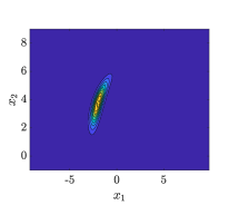
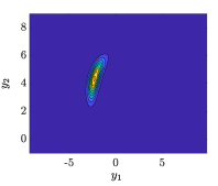
Figure 7: Solution to the linear advection equation (90) with coefficients (93) at time $t=30$. (a) Cartesian coordinates, (b) tensor ridge simulation 1 using on Algorithm 3 with $\Delta\epsilon=10^{-4}$, $M_{\rm iter}=2000$, and ${\eta}=10^{-1}$, (c) tensor ridge simulation 2 using Algorithm 4 with $M_{\rm iter}=1$ and $\Delta\epsilon=10^{-3}$. In all simulations the truncation tolerance is set to $10^{-6}$.

In the first example, we generate the vector field $\bm{f}(\bm{x})=(f_{1}(\bm{x}),f_{2}(\bm{x}))$ via the two-dimensional stream function [46]

$$\psi(x_{1},x_{2})=\Theta(x_{1})\Theta(x_{2})$$ (91)

with

$$\Theta(x)=\frac{\cos(\alpha x/L)}{\cos(\alpha/2)}-\frac{\cosh(\alpha x/L)}{\cosh(\alpha/2)},$$ (92)

$L=30$ and $\alpha=4.73$. Such a stream function generates the divergence-free vector field (see Figure 9(a))

$$f_{1}(\bm{x})=\frac{\partial\psi}{\partial x_{2}},\qquad f_{2}(\bm{x})=-\frac{\partial\psi}{\partial x_{1}}.$$ (93)

We set the initial condition

$$u_{0}(\bm{x})=\frac{1}{m}\exp\left(-4(x_{1}-2)^{2}\right)\exp\left(-\frac{(x_{2}-2)^{2}}{2}\right),$$ (94)

where

$$m=\left\|\exp\left(-4(x_{1}-2)^{2}\right)\exp\left(-\frac{(x_{2}-2)^{2}}{2}\right)\right\|_{L^{2}(\Omega)}$$

is a normalization constant.

We first ran one rank-adaptive tensor simulation in fixed Cartesian coordinates. We then ran two coordinate-adaptive simulations that use rank-reducing coordinate transformations during time integration. In the first coordinate-adaptive simulation we use Algorithm 3 with ${\rm max\ rank}=15$ and $k_{r}=0$ to initialize coordinate transformations during time integration. For the Riemannian gradient descent algorithm that computes the rank reducing coordinate transformation we set step-size $\Delta\epsilon=10^{-4}$, maximum number of iterations $M_{\rm iter}=2000$ and stopping tolerance ${\eta}=10^{-1}$. In the second coordinate-adaptive simulation we use Algorithm 4 with $M_{\rm iter}=1$ and $\Delta\epsilon=10^{-3}$, i.e., the integrator performs one step of time integration followed by one step of the Riemannian gradient descent algorithm 1. In both coordinate-adaptive simulations we set the truncation threshold $\delta=10^{-6}$.

In Figure 7 we plot the solutions obtained from each of the three simulations at time $t=30$. In order to check the accuracy of integrating the PDE solution in the low-rank coordinate system we mapped the transformed solution back to Cartesian coordinates using a two-dimensional trigonometric interpolant and compared with the solution computed in Cartesian coordinates. In both coordinate-adaptive simulations we found that the global $L^{\infty}$ error is bounded by $8\times 10^{-4}$, suggesting that the coordinate transformation does not affect accuracy significantly. In Figure 8 we plot the solution rank and the rank of the of the right hand side of the PDE (90) versus time for all three tensor simulations. We observe that in the coordinate-adaptive tensor ridge simulations the ranks of both the solution and the PDE right hand side are less than or equal to the corresponding ranks in Cartesian coordinates. We also observe that the adaptive simulation based on Algorithm 4 (denoted by “tensor ridge 2” in Figure 8) has significantly smaller rank than the adaptive simulation based on Algorithm 3 (denoted by “tensor ridge 1” in Figure 8).

     (a)                                                                (b)

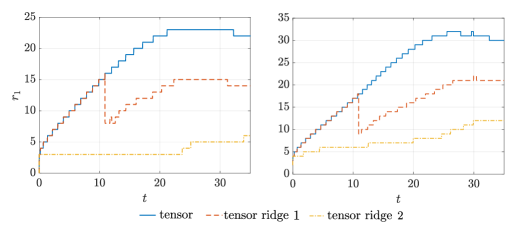
Figure 8: 2D Linear advection equation (90) with coefficients (93). Rank (number of singular values larger than $\delta=10^{-6}$) of the PDE solution (a) and the right hand side the PDE (b). Tensor ridge 1 was computed using Algorithm 3 with a maximum solution rank threshold of $15$. Tensor ridge 2 was computed using Algorithm 4, which performs coordinate corrections at each time step.

Next, we demonstrate that linear coordinate transformations can be used to reduce the rank of a PDE operator and reduce the overall computational cost of temporal integration. To this end, consider again the two-dimensional advection equation (90) this time with advection coefficients

$$f_{1}(\bm{x}) =\exp\left(-a_{1}\left(\bm{R}_{1}\cdot\bm{x}\right)^{2}\right)\exp\left(-a_{2}\left(\bm{R}_{2}\cdot\bm{x}\right)^{2}\right),$$ (95)

$$f_{2}(\bm{x}) =\exp\left(-b_{1}\left(\bm{R}_{1}\cdot\bm{x}\right)^{2}\right)\exp\left(-b_{2}\left(\bm{R}_{2}\cdot\bm{x}\right)^{2}\right),$$

where $\bm{R}_{i}$ is the $i^{\text{th}}$ row of the matrix $\bm{R}$,

$$\bm{R}=\begin{bmatrix}\cos(\theta)&-\sin(\theta)\\ \sin(\theta)&\cos(\theta)\end{bmatrix}.$$ (96)

We set parameters $\theta=\pi/4$,

$$a_{1}=1/20,\quad a_{2}=1/10,\quad b_{1}=1/10,\quad b_{2}=1/20,$$ (97)

and initial condition

$$u_{0}(\bm{x})=\exp\left(-x_{1}^{2}/3\right)\exp\left(-x_{2}^{2}/3\right).$$ (98)

In Figure 9(b) we plot the vector field $\bm{f}(\bm{x})=(f_{1}(\bm{x}),f_{2}(\bm{x}))$ defined by (95). Note that the initial condition $u_{0}(\bm{x})$ is rank $1$. The rank of the linear advection operator defined on the right hand side of (90) depends on the FTT truncation tolerance used to compress the multivariate functions $f_{1}(\bm{x})$ and $f_{2}(\bm{x})$. If we choose the coordinate transformation $\bm{y}=\bm{\Gamma}\bm{x}$, where $\bm{\Gamma}=\bm{R}^{-1}$, then the initial condition remains rank 1, but the rank of the advection operator at the right hand side of (90) becomes 2, regardless of the FTT truncation tolerance used.

    (a)                                                                  (b)

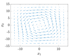
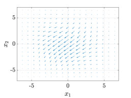
Figure 9: (a) Vector fields used as coefficients in the two-dimensional linear advection equation (90). The vector field defined in (93) is shown in (a) and the vector field defined in (95) is shown in (b).

We ran two simulations of (90) with coefficients (95) using the step-truncation FTT integrator (49) based on Adams-Bashforth 3 with step-size $\Delta t=10^{-3}$, truncation tolerance $\delta=10^{-6}$, and final integration time $t=5$. In the first simulation we solved the PDE with a step-truncation tensor method in fixed Cartesian coordinates. In the second simulation we solved the PDE in coordinates $\bm{y}=\bm{R}^{-1}\bm{x}$, using the same step-truncation tensor method. In order to verify the accuracy of our FTT simulations we also computed a benchmark solution on a full tensor product grid in two dimensions. We then mapped the transformed solution back to Cartesian coordinates at each time step and compared it with the benchmark solution. We found that the global $L^{\infty}$ error of both low-rank simulations is bounded by $8\times 10^{-4}$. In Figure 10 we plot the FTT solution in Cartesian coordinates and the FTT-ridge solution in low-rank coordinates at time $t=5$. We observe that the PDE operator expressed in Cartesian coordinates advects the solution at an angle relative to the underling coordinate system while the operator expressed in coordinates $\bm{y}=\bm{R}^{-1}\bm{x}$ advects the solution directly along a coordinate axis, hence the low rank dynamics. In Figure 12(a) we plot the solution ranks versus time. Note that even though the operator in Cartesian coordinates has significantly larger rank than the operator in low-rank coordinates, the solution ranks follow the same trend during temporal integration with the FTT-ridge rank only slightly smaller than the FTT rank.

Computational cost

The CPU-time of integrating the advection equation (90) with coefficients (95) from $t=0$ to $t=5$ is 72 seconds when computed with FTT in Cartesian coordinates and 31 seconds when computed with FTT-ridge in low-rank coordinates. Note that although the ranks of the low-rank solutions are similar at each time step (Figure 12(a)), the computational speed-up of the FTT-ridge simulation is due to the operator rank, which is $2$ for FTT-ridge and $16$ for FTT in Cartesian coordinates.

(a)                                                                        (b)

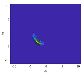
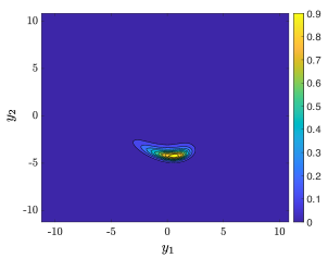
Figure 10: Solution to the two-dimensional advection equation (90) with coefficients (95) at time $t=5$. (a) FTT solution computed in Cartesian coordinates. (b) FTT-ridge computed low-rank coordinates.

6.5 Allen-Cahn equation

Next we demonstrate coordinate-adaptive tensor integration on a simple nonlinear PDE. The Allen-Cahn eqaution is a reaction-diffusion PDE, which, in its simplest form includes a low-order polynomial non-linearity (reaction term) and a diffusion term [20]

$$\begin{cases}\displaystyle\frac{\partial u(\bm{x},t)}{\partial t}=\alpha\Delta u(\bm{x},t)+u(\bm{x},t)-u(\bm{x},t)^{3},\\ u(\bm{x},0)=u_{0}(\bm{x}).\end{cases}$$ (99)

In two spatial dimensions the Laplacian in coordinates $\bm{y}=\bm{\Gamma}\bm{x}$ is given by

$$\Delta_{\bm{\Gamma}}= \left(\Gamma_{11}^{2}+\Gamma_{12}^{2}\right)\frac{\partial^{2}}{\partial y_{1}^{2}}+\left(\Gamma_{21}^{2}+\Gamma_{22}^{2}\right)\frac{\partial^{2}}{\partial y_{2}^{2}}+2\left(\Gamma_{11}\Gamma_{21}+\Gamma_{12}\Gamma_{22}\right)\frac{\partial^{2}}{\partial y_{1}\partial y_{2}}$$ (100)

which allows us to write the nonlinear PDE (99) in the coordinate system $\bm{y}=\bm{\Gamma}\bm{x}$ with only a small increase in the rank of the Laplacian operator. The FTT rank of the cubic term appearing in the PDE operator of the Allen-Cahn equation (99) is determined by the rank of the FTT solution. Standard algorithms for multiplying two FTT tensors $u_{\text{\tiny TT}}$ and $v_{\text{\tiny TT}}$ with ranks $\bm{r}_{1}$ and $\bm{r}_{2}$ results in a FTT tensor with (non-optimal) rank equal to the Hadamard product of the two ranks $\bm{r}_{1}\circ\bm{r}_{2}$. Hence, by reducing the solution rank with a coordinate transformation, we can reduce the computational cost of computing the nonlinear term in (99). We set the diffusion coefficient $\alpha=0.2$ and the initial condition $u_{0}(\bm{x})$ as the rotated Gaussian from equation (25) with $\epsilon=\pi/3$.

We ran two FTT simulations of (99) for time $t\in[0,5]$. The first simulation was computed in fixed Cartesian coordinates. In the second simulation we used the coordinate transformation $\bm{\Phi}(\pi/3)^{-1}$ (which in this case we have available analytically) to transform the initial condition into a rank 1 FTT-ridge function. We integrated the rank 1 FTT-ridge initial condition forward in time using the corresponding transformed PDE, i.e., using the transformed Laplacian (100). In order to verify the accuracy of our low-rank simulations we also computed a benchmark solution on a full tensor product grid in two dimensions and mapped the transformed solution back to Cartesian coordinates at each time step. We found that the global $L^{\infty}$ error of both low-rank solutions is bounded $5\times 10^{-5}$. In Figure 11 we plot the FTT solution in Cartesian coordinates and the FTT-ridge solution in low-rank coordinates at time $t=5$. We observe that the profile of Gaussian functions are preserved as the solution moves from the unstable equilibrium at $u=0$ to the stable equilibrium at $u=1$.

(a)                                                                         (b)

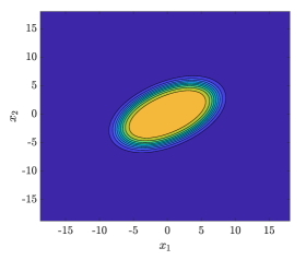
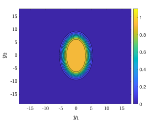
Figure 11: Solution to the two-dimensional Allen-Cahn equation (99) at time $t=5$. (a) FTT solution computed in Cartesian coordinates and (b) FTT-ridge solution computed in low-rank coordinates.

In Figure 12(b) we plot the solution ranks versus time. We observe that the FTT solution rank is larger than the FTT-ridge solution rank at each time.

Computational cost

The CPU-time of integrating the Allen-Cahn equation (99) from $t=0$ to $t=5$ is 279 seconds when computed using FTT in Cartesian coordinates and 72 seconds when computed using FTT-ridge in low-rank coordinates. The optimal coordinate transformation at time $t=0$ is known analytically so we do not need to compute it, thus these computational timings only include the temporal integration, and do not account for any computational time of changing the coordinate system. A significant amount of computational time in computing the FTT solutions comes from computing the cubic nonlinearity appearing in the Allen-Cahn equation at each time step. The lower rank FTT-ridge solution allows for this term to be computed significantly faster than the FTT solution in Cartesian coordinates.

6.6 3D and 5D linear advection equations

We also applied the rank-reducing coordinate-adaptive FTT integrators to the advection equation

$$\begin{cases}\displaystyle\frac{\partial u(\bm{x},t)}{\partial t}=\bm{f}(\bm{x})\cdot\nabla u(\bm{x},t),\vspace{0.2cm}\\ u(\bm{x},0)=u_{0}(\bm{x}),\end{cases}$$ (101)

in dimensions three and five with initial condition $u_{0}(\bm{x})$ defined as a Gaussian mixture

$$u_{0}(\bm{x})=\frac{1}{m}\sum_{i=1}^{N_{g}}\exp\left(-\sum_{j=1}^{d}\frac{1}{\beta_{ij}}\left(\bm{R}^{(i)}_{j}\cdot\bm{x}+t_{ij}\right)^{2}\right),$$ (102)

where $\bm{R}_{j}{{}^{(i)}}$ is the $j$-th row of a $d\times d$ rotation matrix $\bm{R}{{}^{(i)}}$, $\beta_{i}\geq 0$, $t_{ij}$ are translations and $m$ is the normalization factor

$$m=\left\|\sum_{i=1}^{N_{g}}\exp\left(-\sum_{j=1}^{d}\frac{1}{\beta_{ij}}\left(\bm{R}^{(i)}_{j}\cdot\bm{x}+t_{ij}\right)^{2}\right)\right\|_{L^{1}\left(\mathbb{R}^{d}\right)}.$$

         (a)                                                                                            (b)

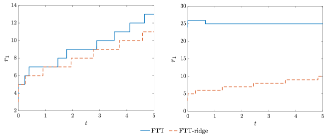
Figure 12: (a) Rank versus time for the FTT and FTT-ridge solutions to the advection PDE (90) with coefficients (95). (b) Rank versus time for the FTT and FTT-ridge solutions to the Allen-Cahn equation (99).

6.6.1 Three-dimensional simulation results

First, we consider three spatial dimensions ($d=3$), and set the coefficients in (101) as

$${\bm{f}(\bm{x})}=-\frac{1}{6}\begin{bmatrix}2\sin(x_{2})\\ 3\cos(x_{3})\\ 3x_{1}\\ \end{bmatrix},$$ (103)

resulting in the linear operator

          $t=0$                                                                                $t=1$

FTT (Cartesian coordinates)

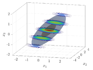
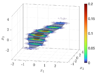
FTT-ridge (low-rank coordinates)

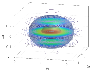
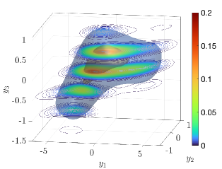
Figure 13: Volumetric plot of the FTT solutions to the 3D advection equation (101) at time $t=0$ (left column) in Cartesian coordinates (top) and low-rank coordinates (bottom), and at time $t=1$ (right column) in Cartesian coordinates (top) and low-rank coordinates (bottom).

$${\bm{f}(\bm{x})\cdot\nabla}=\frac{\sin(x_{2})}{3}\frac{\partial}{\partial x_{1}}+\frac{\cos(x_{3})}{2}\frac{\partial}{\partial x_{2}}+\frac{x_{1}}{2}\frac{\partial}{\partial x_{3}}.$$ (104)

In a previous work [12] we have demonstrated that variable coefficient advection problems with operators of the form (104) can have solutions with multilinear rank that grows significantly over time. We set the parameters in the initial condition (102) $N_{g}=1$,

$$\bm{R}^{(1)}=\exp\left(\frac{1}{28}\begin{bmatrix}0&7\pi&4\pi\\ -7\pi&0&7\pi\\ -4\pi&-7\pi&0\end{bmatrix}\right),\qquad\bm{\beta}=\begin{bmatrix}3&{1}/{10}&3\end{bmatrix},$$ (105)

and $t_{ij}=0$ for all $i,j$.

       (a)                                                        (b)                                                        (c)

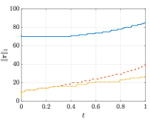
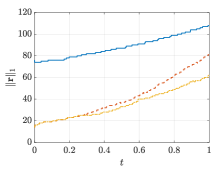
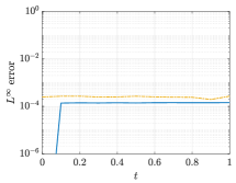
Figure 14: 3D advection equation (101): Multilinear rank of the PDE solution (a) and PDE right-hand-side (b) in Cartesian coordinates and transformed coordinates versus time. In (c) we plot the $L^{\infty}$ error of the FTT solutions relative to a benchmark solution.

We ran three FTT simulations up to time $t=1$. The first simulation is computed in fixed Cartesian coordinates. We then tested the FTT integrator with rank-reducing coordinate transformation in two different simulation settings. In the first one, we performed a coordinate transformation only at time $t=0$. Such a coordinate transformation is not done using the Riemannian gradient descent algorithm, since, in this case we have the optimal coordinate transformation available analytically and we can simply evaluate the FTT tensor on the low rank coordinates. In the second simulation we also performed a coordinate transformation at time $t=0$ (once again the coordinate transformation at time $t=0$ is not done using the Riemannian gradient descent algorithm) and then used the coordinate-adaptive integration Algorithm 3 with ${\rm max\ rank}=15$ and $k_{r}=5$. With these parameters the coordinate-adaptive algorithm triggers three additional coordinate transformations at times $t\in\{0.25,0.59,0.9\}$ that are computed using the Riemannian gradient descent algorithm 1 with step size $\Delta\epsilon=10^{-4}$ and stopping tolerance ${\eta}=10^{-1}$. In Figure 15(c) we plot the absolute value of the derivative of the cost function $C(\bm{\Gamma}(\epsilon))$ versus $\epsilon$ for the instances of gradient descent at times $t>0$. We observe that the rate of change of the cost function becomes smaller as we iterate the gradient descent routine, i.e., the cost function is decreasing less per iteration after several iterations. This indicates that the cost function is approaching a flatter region and our gradient descent method is becoming less effective for reducing the cost function. In Figure 14(a) we plot the $1$-norm of the FTT solution rank vector versus time and in Figure 14(b) we plot the $1$-norm of the FTT solution velocity (i.e., the PDE right hand side) for each FTT simulation. We observe that the FTT-ridge solutions and right hand side of the PDE have rank that is smaller than the corresponding ranks of the FTT solution in Cartesian coordinates. We also observe that the adaptive coordinate transformations performed at times $t>0$ do not reduce the solution rank at the time of application, but they do slow the rank increase as time integration proceeds. In Figure 15(a)-(b) we plot the singular values of the FTT solutions at final time and note that both FTT-ridge solutions have singular values that decay significantly faster than the FTT solution in Cartesian coordinates. Moreover, the additional coordinate transformations performed by the coordinate-adaptive integrator causes the singular values of the FTT-ridge solution to decay faster than the other FTT-ridge solution that used only one coordinate transformation at $t=0$. In Figure 13 we provide volumetric plots of the PDE solution in Cartesian coordinates and in the transformed coordinate system computed with the coordinate-adaptive algorithm 3 at time $t=1$. We observe that the reduced rank tensor ridge solution appears to be more symmetrical with respect to the underlying coordinate axes than the solution in Cartesian coordinates.

It is important to note that the operator $G(\cdot,\bm{x})=\bm{f}(\bm{x})\cdot\nabla$ in (104) is a separable operator of rank $\bm{g}=\begin{bmatrix}1&3&3&1\end{bmatrix}$. For a general linear coordinate transformation $\bm{\Gamma}$ the operator $G_{\bm{\Gamma}}$ (see (82)) acting in the transformed coordinate system can be obtained using trigonometric identities with (non-optimal) separation ranks. A more efficient representation of $G_{\bm{\Gamma}}$ can be obtained by FTT compression and then splitting $G_{\bm{\Gamma}}$ (77) into a sum of three operators

$$G_{\bm{\Gamma}}=G_{\bm{\Gamma}}^{(1)}+G_{\bm{\Gamma}}^{(2)}+G_{\bm{\Gamma}}^{(3)},$$ (106)

where $G_{\bm{\Gamma}}^{(i)}$ have ranks $\bm{g}_{\bm{\Gamma}}^{(i)}=\begin{bmatrix}1&4&4&1\end{bmatrix}$ for each $i=1,2,3$. Then we apply the operator $G_{\bm{\Gamma}}$ to the FTT-ridge solution at each time using the procedure summarized in (78). In this case, since the PDE operator $G$ in Cartesian coordinates is separable and low-rank, it is not surprising that a linear coordinate transformation increases the PDE operator rank. However by splitting the operator such as (106) and performing a FTT truncation operation after applying each lower rank operator $G_{\bm{\Gamma}}^{(i)}$ we can mitigate the computational cost.

               (a)                                                      (b)                                                        (c)

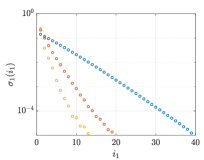
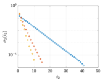
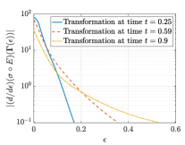
Figure 15: (a)-(b) Multilinear spectra of the FTT solutions to the 3D advection equation (101) at time $t=1$ in Cartesian coordinates and in low-rank coordinates. (c) Absolute value of the derivative of the cost function in (27) during gradient descent of the 3D advection equation (101) solutions at times $t>0$.

In Figure 14(c) we plot the $L^{\infty}$ error between the transformed solutions and the FTT solution in Cartesian coordinates relative to the benchmark solution. We observe that the $L^{\infty}$ error of our coordinate-adaptive solution is very close to the $L^{\infty}$ error of the solution computed in Cartesian coordinates. This implies that the error incurred by transforming coordinates, integrating the PDE in the new coordinate system, and then transforming coordinates back is not significant.

Computational cost

The CPU-time of integrating the three-dimensional advection equation (101) from $t=0$ to $t=1$ is 413 seconds when computed using FTT in Cartesian coordinates, 173 seconds when computed using FTT-ridge in low-rank coordinates with one coordinate transformation at $t=0$, and 299 seconds when computed using the coordinate-adaptive FTT Algorithm 3. These timings do not include the coordinate transformations at time $t=0$ since they were not computed using Riemannian gradient descent. The timings do include the computation of the new coordinate systems at times $t>0$.

  $t=0$                                                                              $t=1$

FTT (Cartesian coordinates)

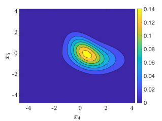
FTT-ridge (transformed coordinates)

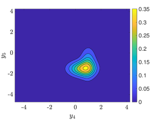
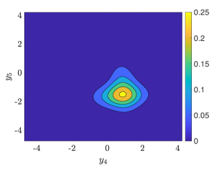
Figure 16: Marginal PDFs of the solution to the 5D advection equation (101) computed in Cartesian coordinates and low-rank adaptive coordinates at time $t=0$ and time $t=1$.

6.6.2 Five-dimensional simulation results

Finally, we consider the advection equation (101) in dimension five ($d=5$) with coefficients

$$\bm{f}(\bm{x})=\begin{bmatrix}-x_{2}\\ x_{3}\\ x_{5}\\ -x_{2}\\ -x_{3}\end{bmatrix}.$$ (107)

This allows us to test our coordinate-adaptive algorithm for a case in which we know the optimal ridge matrix.

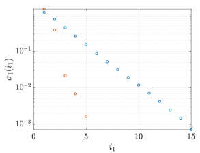
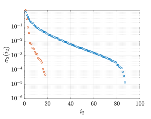
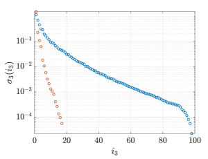
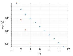
Figure 17: Multilinear spectra of the solution to the advection 5D PDE (101) in Cartesian coordinates and transformed coordinates at time $t=1$.

In the initial condition (102) we set the following parameters: $N_{g}=2$,

$$\bm{R}^{(1)}=\bm{R}^{(2)}=\bm{I}_{5\times 5},$$ (108)

$$\bm{\beta}=\begin{bmatrix}1/2&2&1/2&3&1/2\\ 1&1/3&2&1&1/2\end{bmatrix},$$

and

$$\bm{t}=\begin{bmatrix}1&1&1&-1&1\\ 0&0&3/2&-1/2&1/2\end{bmatrix},$$ (109)

which results in an initial condition with FTT rank $\begin{bmatrix}1&2&2&2&2&1\end{bmatrix}$. Due to the choice of coefficients (107), the analytical solution to the PDE (101) can be written as a ridge function in terms of the PDE initial condition

$$u(\bm{x},t)=u_{0}\left(e^{t\bm{B}}\bm{x}\right),$$ (110)

where

$$\bm{B}=\begin{bmatrix}0&-1&0&0&0\\ 0&0&1&0&0\\ 0&0&0&0&1\\ 0&-1&0&0&0\\ 0&0&-1&0&0\end{bmatrix}.$$ (111)

Thus (110) is a tensor ridge solution to the 5D advection equation (101) with the same rank as the initial condition, i.e., in this case there exists a tensor ridge solution at each time with FTT rank equal to $\begin{bmatrix}1&2&2&2&2&1\end{bmatrix}$.

We ran two simulations of the PDE (101) up to $t=1$. The first simulation is computed with a step-truncation method in fixed Cartesian coordinates. The second simulation is computed with the coordinate-adaptive FTT-ridge tensor method that performs coordinate corrections at each time step (Algorithm 4) with $\Delta\epsilon=5\times 10^{-4}$ and $M_{\rm iter}=1$. In Figure 16 we plot marginal PDFs of the FTT solution and the FTT-ridge solution at initial time $t=0$ and final time $t=1$. We observe that the reduced rank FTT-ridge solution appears to be more symmetrical with respect to the coordinate axes than the corresponding function on Cartesian coordinates. In Figure 18(a) we plot the $1$-norm of the FTT solution rank versus time and in Figure 18(b) we plot the FTT rank of the PDE velocity vector (right hand side of the PDE) versus time for both FTT solutions. We observe that the FTT solution rank in Cartesian coordinates grows quickly compared to the FTT-ridge solution in Cartesian coordinates. This is expected due to the existence of a low-rank FTT-ridge solution (110). Note that the coordinate-adaptive algorithm 4 produces a FTT-ridge solution with ridge matrix that is different than $e^{t\bm{B}}$ in (110). The reason can be traced back to the cost function we are minimizing, i.e., the Schauder norm (see section 4.1), and the fact that we do not fully determine the minimizer at each step, but rather perform only one $\epsilon$-step in the direction of the Riemannian gradient. Although the rank of the FTT-ridge solution computed with algorithm 4 is larger than the rank of the analytical solution (110), the algorithm still controls the FTT solution rank during time integration. In Figure 17 we plot the multilinear spectra of the two FTT solutions at time $t=1$. We observe that the multilinear spectra of the FTT-ridge function decay significantly faster than the spectra of the FTT solution in Cartesian coordinates.

For this problem it is not straightforward to compute a benchmark solution on a full tensor product grid. If we were to use the same resolution as the FTT solutions, i.e., $200$ points in each dimension, then each time snapshot of the benchmark solution would be an array containing $200^{5}\approx 3.2\times 10^{11}$ double precision floating point numbers. This requires $2.56$ terabytes of memory storage per time snapshot. In lieu of comparing our FTT solutions with a benchmark solution, we compared the two FTT solutions with each other. To do so we mapped the FTT-ridge solution back to Cartesian coordinates every $250$ time steps by solving a PDE of the form (20) numerically. We compared the $(x4,x5)$-marginal PDFs of the two solutions and found that the global $L^{\infty}$ norm of the difference of the two solution PDFs is bounded by $6\times 10^{-4}$.

                                                            (a)                                                                             (b)

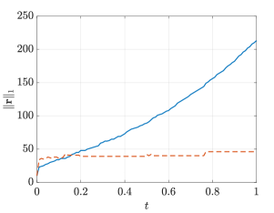
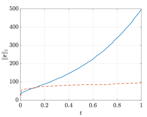
Figure 18: (a) 1-norm of the solution rank vectors versus time. (b) 1-norm of the solution velocity (PDE right hand side) rank vectors versus time.

Computational cost

The CPU-time of integrating the five-dimensional advection equation (101) from $t=0$ to $t=1$ is 2046 seconds when computed using FTT in Cartesian coordinates and 2035 seconds when computed using FTT-ridge in low-rank coordinates with coordinate corrections at each time step.

Appendix A The Riemannian manifold of coordinate transformations

We endow the search space ${\rm SL}_{d}(\mathbb{R})$ in (38) with a Riemannian manifold structure. To this end, we first notice that ${\rm SL}_{d}(\mathbb{R})$ is a matrix Lie group over $\mathbb{R}$ and in particular is a smooth manifold. A point $\bm{A}\in{\rm SL}_{d}(\mathbb{R})$ corresponds to a linear coordinate transformation of $\mathbb{R}^{d}$ with determinant equal to $1$. A smooth path $\bm{\Theta}(\epsilon)$ on the manifold ${\rm SL}_{d}(\mathbb{R})$ paramaterized by $\epsilon\in(-\delta,\delta)$ is a collection of smoothly varying linear coordinate transformations with determinant equal to $1$ for all $\epsilon\in(-\delta,\delta)$. Denote by $\mathcal{C}^{1}\left((-\delta,\delta),{\rm SL}_{d}(\mathbb{R})\right)$ the collection of all continuously differentiable paths $\bm{\Theta}(\epsilon)$ on the manifold ${\rm SL}_{d}(\mathbb{R})$ parameterized by $\epsilon\in(-\delta,\delta)$. The tangent space of ${\rm SL}_{d}(\mathbb{R})$ at the point $\bm{A}\in{\rm GL}_{d}(\mathbb{R})$ is defined to be the collection of equivalence classes of velocities associated to all possible curves on ${\rm SL}_{d}(\mathbb{R})$ passing through the point $\bm{A}$

$$T_{\bm{A}}{\rm SL}_{d}(\mathbb{R})=\left\{\frac{d\bm{\Theta}(\epsilon)}{d\epsilon}\biggr{|}_{\epsilon=0}:\quad\bm{\Theta}\in\mathcal{C}^{1}\left((-\delta,\delta),{\rm SL}_{d}(\mathbb{R})\right),\quad\bm{\Theta}(0)=\bm{A}\right\}.$$ (112)

It is well-known (e.g., [40]) that the tangent space of ${\rm SL}_{d}(\mathbb{R})$ at the point $\bm{A}$ is given by

$$T_{\bm{A}}{\rm SL}_{d}(\mathbb{R})=\mathfrak{sl}_{d}(\mathbb{R})\bm{A}=\{\bm{N}\bm{A}:\bm{N}\in\mathfrak{sl}_{d}(\mathbb{R})\},$$ (113)

where $\mathfrak{sl}_{d}(\mathbb{R})$ denotes the collection of all $d\times d$ real matrices with vanishing trace. We can easily verify that if $\bm{\Theta}(\epsilon)$ is a smooth collection of matrices parameterized by $\epsilon\in(-\delta,\delta)$ with $\bm{\Theta}(0)\in{\rm SL}_{d}(\mathbb{R})=\mathfrak{sl}_{d}(\mathbb{R})$ and $d\bm{\Theta}(\epsilon)/d\epsilon\in T_{\bm{\Theta}(\epsilon)}{\rm SL}_{d}(\mathbb{R})$ for all $\epsilon$, then $\det(\bm{\Theta}(\epsilon))=1$ for all $\epsilon$, i.e., $\bm{\Theta}(\epsilon)\in{\rm SL}_{d}(\mathbb{R})$ for all $\epsilon$. The proof of this result is a direct application of Jacobi’s formula [30] which states

$$\frac{d}{d\epsilon}\det\left(\bm{\Theta}(\epsilon)\right) =\det\left(\bm{\Theta}(\epsilon)\right){\rm trace}\left(\frac{d\bm{\Theta}(\epsilon)}{d\epsilon}\bm{\Theta}^{-1}(\epsilon)\right)$$ (114)

$$=\det\left(\bm{\Theta}(\epsilon)\right){\rm trace}\left(\bm{N}\bm{\Theta}(\epsilon)\bm{\Theta}^{-1}(\epsilon)\right)$$

$$=\det\left(\bm{\Theta}(\epsilon)\right){\rm trace}\left(\bm{N}\right)$$

$$=0,$$

since $\bm{N}\in\mathfrak{sl}_{d}(\mathbb{R})$. Thus the determinant of $\bm{\Theta}(\epsilon)$ is constant and since $\det(\bm{\Theta}(0))=1$ it follows that $\det(\bm{\Theta}(\epsilon))=1$ for all $\epsilon\in(-\delta,\delta)$. In the language of abstract differential equations, $\mathfrak{sl}_{d}(\mathbb{R})$ is referred to as the Lie algebra associated with the Lie group ${\rm SL}_{d}(\mathbb{R})$. In Figure 19(a) we provide an illustration of a path $\bm{\Theta}(\epsilon)$ on the manifold ${\rm SL}_{d}(\mathbb{R})$ passing through the point $\bm{A}$ and the tangent space $T_{\bm{A}}{\rm SL}_{d}(\mathbb{R})$ of ${\rm SL}_{d}(\mathbb{R})$ at $\bm{A}$. Also depicted in Figure 19 is a smooth function $f$ from ${\rm SL}_{d}(\mathbb{R})$ to another smooth manifold $\mathcal{M}$. The image of the path $\bm{\Theta}(\epsilon)$ on $\rm{SL}_{d}(\mathbb{R})$ under $f$ is a path $f(\bm{\Theta}(\epsilon))$ on $\mathcal{M}$. Under this mapping of curves, we can associate the tangent vector $d\bm{\Theta}(\epsilon)/d\epsilon|_{\epsilon=0}$ in $T_{\bm{A}}{\rm SL}_{d}(\mathbb{R})$ with a tangent vector $df(\bm{\Theta}(\epsilon))/d\epsilon|_{\epsilon=0}$ in $T_{f(\bm{A})}\mathcal{M}$. This association gives rise to the notion of the directional derivative of a function $f:{\rm SL}_{d}(\mathbb{R})\to\mathcal{M}$ which we now define.

Definition A1. Let $f$ be a smooth function from the Riemannian manifold ${\rm SL}_{d}(\mathbb{R})$ to a smooth manifold $\mathcal{M}$. The directional derivative of $f$ at the point $\bm{A}\in{\rm SL}_{d}(\mathbb{R})$ in the direction $\bm{V}\in T_{\bm{A}}{\rm SL}_{d}(\mathbb{R})$ is defined as

$$(d_{\bm{A}}f)\bm{V}=\frac{\partial f(\bm{\Theta}(\epsilon))}{\partial\epsilon}\biggr{|}_{\epsilon=0},$$ (115)

where $\bm{\Theta}(\epsilon)$ is a smooth curve on ${\rm SL}_{d}(\mathbb{R})$ passing through the point $\bm{A}$ at $\epsilon=0$ with velocity $\bm{V}$.

It is a standard exercise of differential geometry to verify that the directional derivative (115) is independent of the choice of curve $\bm{\Theta}(\epsilon)$. The map $d_{\bm{A}}f$ appearing in (115) is a linear map from $T_{\bm{A}}{\rm SL}_{d}(\mathbb{R})$ to $T_{f(\bm{A})}\mathcal{M}$ known as the differential of $f$.

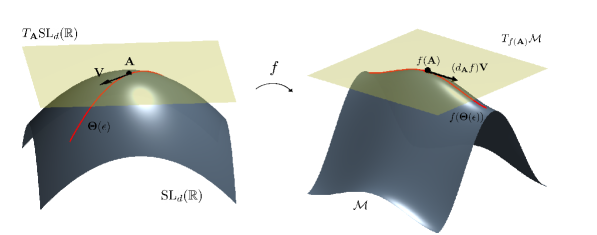
Figure 19: An illustration of the directional derivative of the function $f:{\rm SL}_{d}(\mathbb{R})\to\mathcal{M}$. The curve $\bm{\Theta}(\epsilon)$ on ${\rm SL}_{d}(\mathbb{R})$ is mapped to the curve $f(\bm{\Theta}(\epsilon))$ on $\mathcal{M}$ and the directional derivative of $f$ at $\bm{A}\in{\rm SL}_{d}(\mathbb{R})$ in the direction $\bm{V}\in T_{\bm{A}}{\rm SL}_{d}(\mathbb{R})$ is the velocity of the curve $f(\bm{\Theta}(\epsilon))$ at $f(\bm{A})$.

In Figure 19 we provide an illustration of the mapping $f$ and its differential. The differential and directional derivative allow us to understand the change in $f$ when moving from the point $\bm{A}\in{\rm SL}_{d}(\mathbb{R})$ in the direction of the tangent vector $\bm{V}\in T_{\bm{A}}{\rm SL}_{d}(\mathbb{R})$. Next, we compute the Riemannian gradient of $f$, i.e., a specific tangent vector on ${\rm SL}_{d}(\mathbb{R})$ that points in a direction which makes the function $f$ vary the most.

For functions defined on Euclidean space, the connection between directional derivative and gradient is understood by using the standard inner product defined for Euclidean spaces. A generalization of the Euclidean inner product for an abstract manifold such as ${\rm SL}_{d}(\mathbb{R})$ is the Riemannian metric $(\cdot,\cdot)_{\bm{A}}$, which is a collection of smoothly varying inner products on each tangent space $T_{\bm{A}}{\rm SL}_{d}(\mathbb{R})$. In particular, we define

$$(\bm{V},\bm{W})_{\bm{A}}={\rm trace}\left[\left(\bm{V}\bm{A}^{-1}\right)\left(\bm{W}\bm{A}^{-1}\right)^{\text{T}}\right],\qquad\forall\bm{A}\in{\rm SL}_{d}(\mathbb{R}),\quad\forall\bm{V},\bm{W}\in T_{\bm{A}}{\rm SL}_{d}(\mathbb{R})$$ (116)

on ${\rm SL}_{d}(\mathbb{R})$. With this Riemannian metric, we can define the Riemannian gradient.

Definition A2. Let $f$ be a smooth function from ${\rm SL}_{d}(\mathbb{R})$ to a smooth manifold $\mathcal{M}$. The Riemannian gradient of $f$ at the point $\bm{A}\in{\rm SL}_{d}(\mathbb{R})$ is the unique vector field ${\rm grad}f(\bm{A})$ satisfying

$$(d_{\bm{A}}f)\bm{V}=({\rm grad}f(\bm{A}),\bm{V})_{\bm{A}},\qquad\forall\bm{V}\in T_{\bm{A}}{\rm SL}_{d}(\mathbb{R}).$$ (117)

Analogous to the Euclidean case, the Riemannian gradient points in the direction which $f$ increases the most, and, the negative gradient points the the direction which $f$ decreases most. With this Riemannian geometric structure, we proceed by constructing a path on ${\rm SL}_{d}(\mathbb{R})$, known as a descent path, which converges to a local minimum of the cost function $S\circ E$ in (38).

Appendix B Theorems and Proofs

First, we show that the tensor rank is invariant under translation of functions with compact support. This allows us to disregard translations when looking for rank reducing coordinate flows.

Proposition B1.

Let $u_{\text{\tiny TT}}\in L^{2}_{\mu}(\Omega)$ $(\Omega\subseteq\mathbb{R}^{d})$ be a rank-$\bm{r}$ FTT with ${\rm supp}(u_{\text{\tiny TT}})\subseteq\Omega$ and $C_{\bm{t}}:\mathbb{R}^{d}\to\mathbb{R}^{d}$ a coordinate translation, i.e.,

$$C_{\bm{t}}(\bm{x})=\bm{x}+\bm{t},$$ (118)

where $\bm{t}\in\mathbb{R}^{d}$, such that ${\rm supp}(u_{\text{\tiny TT}})\subseteq C_{\bm{t}}(\Omega)$. Then $u_{\text{\tiny TT}}(C_{\bm{t}}(\bm{x}))$ is also a rank-$\bm{r}$ FTT tensor.

Proof. Let

$$u_{\text{\tiny TT}}(\bm{x})=\bm{Q}_{\leq i}(\bm{x}_{\leq i})\bm{\Sigma}_{i}\bm{Q}_{>i}(\bm{x}_{>i})$$ (119)

be an orthogonalized expansion of the the rank-$\bm{r}$ FTT $u_{\text{\tiny TT}}$ as in (28). Then by a simple change of variables in the integrals it is easy to verify that the translated cores $\bm{Q}_{\leq i}^{\text{T}}(\bm{x}_{\leq i}+\bm{t}_{\leq i}),\bm{Q}_{>i}(\bm{x}_{>i}+\bm{t}_{>i})$ also satisfy the orthogonality conditions

$$\left\langle\bm{Q}_{\leq i}^{\text{T}}(\bm{x}_{\leq i}+\bm{t}_{\leq i})\bm{Q}_{\leq i}(\bm{x}_{\leq i}+\bm{t}_{\leq i})\right\rangle_{\leq i}=\bm{I}_{\bm{r}_{i}\times r_{i}},$$ (120)

$$\left\langle\bm{Q}_{>i}(\bm{x}_{>i}+\bm{t}_{>i})\bm{Q}_{>i}^{\text{T}}(\bm{x}_{>i}+\bm{t}_{>i})\right\rangle_{>i}=\bm{I}_{\bm{r}_{i}\times r_{i}},$$

and thus

$$u_{\text{\tiny TT}}(C_{\bm{t}}(\bm{x}))=\bm{Q}_{\leq i}(\bm{x}_{\leq i}+\bm{t}_{\leq i})\bm{\Sigma}_{i}\bm{Q}_{>i}(\bm{x}_{>i}+\bm{t}_{>i})$$ (121)

is an orthogonalized FTT tensor. Hence, $u_{\text{\tiny TT}}\circ C_{\bm{t}}$ has the same multilinear rank $\bm{r}$ as $u_{\text{\tiny TT}}$.

∎

Next, we provide a proof of Proposition 4.1. To do so we first provide the differentials of the maps $E$, $S$ and $C=S\circ E$ in the following lemmas.

Lemma B1.

The differential of the evaluation map $E$ corresponding to ${u_{\text{\tiny TT}}}$ (see eqn. (36)) at the point $\bm{A}\in{\rm GL}_{d}(\mathbb{R})$ in the direction $\bm{V}\in T_{\bm{A}}{\rm GL}_{d}(\mathbb{R})$ is

$$(d_{\bm{A}}E)\bm{V}=\nabla v(\bm{x})\cdot(\bm{V}\bm{x}).$$ (122)

Proof. This result is proven directly from the definitions. Let $\bm{\Theta}(\epsilon)$ be a smooth curve on ${\rm GL}_{d}(\mathbb{R})$ passing through $\bm{A}$ with velocity $\bm{V}$ at $\epsilon=0$. Then

$$(d_{\bm{A}}E)\bm{V} =\frac{\partial}{\partial\epsilon}E(\bm{\Theta}(\epsilon))\biggr{|}_{\epsilon=0}$$ (123)

$$=\frac{\partial}{\partial\epsilon}{u_{\text{\tiny TT}}}(\bm{\Theta}(\epsilon)\bm{x})\biggr{|}_{\epsilon=0}$$

$$=\nabla{u_{\text{\tiny TT}}}(\bm{A}\bm{x})\cdot\left(\bm{V}\bm{x}\right)$$

$$=\nabla v(\bm{x})\cdot\left(\bm{V}\bm{x}\right).$$

∎

Lemma B2.

The differential of $S$ (see (34)) at the point $v\in L^{2}_{\mu}(\Omega)$ in the direction $w\in T_{v}L^{2}_{\mu}(\Omega)$ is

$$(d_{v}S)w=\sum_{i=1}^{d-1}\int_{\Omega}\bm{Q}_{\leq i}\bm{Q}_{>i}w(\bm{x})d\mu(\bm{x})$$ (124)

where $\bm{Q}_{\leq i},\bm{Q}_{>i}$ are FTT cores of $v$ as in eqn. (28) satisfying the orthogonality conditions (31).

Proof. Let $\gamma(\epsilon)$ be a smooth curve on $L^{2}_{\mu}(\Omega)$ passing through $v$ at $\epsilon=0$ with velocity $w$. At each $\epsilon$ the function $\gamma(\epsilon)$ admits orthogonalizations of the form

$$\gamma(\epsilon)=\bm{Q}_{\leq i}(\epsilon)\bm{\Sigma}_{i}(\epsilon)\bm{Q}_{>i}(\epsilon)$$ (125)

for each $i=1,2,\ldots,d-1$. Differentiating (125) with respect to $\epsilon$ we obtain

$$\frac{\partial\gamma}{\partial\epsilon}=\frac{\partial\bm{Q}_{\leq i}}{\partial\epsilon}\bm{\Sigma}_{i}\bm{Q}_{>i}+\bm{Q}_{\leq i}\frac{\partial\bm{\Sigma}_{i}}{\partial\epsilon}\bm{Q}_{>i}+\bm{Q}_{\leq i}\bm{\Sigma}_{i}\frac{\partial\bm{Q}_{>i}}{\partial\epsilon}.$$ (126)

Multiplying on the left by $\bm{Q}_{\leq i}^{\text{T}}$ and on the right by $\bm{Q}_{>i}^{\text{T}}$, applying the operator $\langle\cdot\rangle_{\leq i,>i}$, and evaluating at $\epsilon=0$ we obtain

$$\frac{\partial\bm{\Sigma}_{i}}{\partial\epsilon}=\left\langle\bm{Q}_{\leq i}^{\text{T}}{w}(\bm{x})\bm{Q}_{>i}^{\text{T}}\right\rangle_{\leq i,>i}-\left\langle\bm{Q}_{\leq i}^{\text{T}}\frac{\partial\bm{Q}_{\leq i}}{\partial\epsilon}\right\rangle_{\leq i}\bm{\Sigma}_{i}-\bm{\Sigma}_{i}\left\langle\frac{\partial\bm{Q}_{>i}}{\partial\epsilon}\bm{Q}_{>i}^{\text{T}}\right\rangle_{>i},$$ (127)

where we used orthogonality of the FTT cores $\bm{Q}_{\leq i}$ and $\bm{Q}_{>i}$. Differentiating the orthogonality constraints (31) with respect to $\epsilon$ we obtain

$$\left\langle\frac{\partial\bm{Q}_{\leq i}^{\text{T}}}{\partial\epsilon}\bm{Q}_{\leq i}\right\rangle_{\leq i}=-\left\langle\bm{Q}_{\leq i}^{\text{T}}\frac{\partial\bm{Q}_{\leq i}}{\partial\epsilon}\right\rangle_{\leq i},\qquad\left\langle\frac{\partial\bm{Q}_{>i}}{\partial\epsilon}\bm{Q}_{>i}^{\text{T}}\right\rangle_{>i}=-\left\langle\bm{Q}_{>i}\frac{\partial\bm{Q}_{>i}^{\text{T}}}{\partial\epsilon}\right\rangle_{>i},\quad\forall\epsilon,$$ (128)

which implies that the second two terms on the right hand side of (127) side are skew-symmetric and thus have zeros on the diagonal. Hence the diagonal entries of $\displaystyle\frac{\partial\bm{\Sigma}_{i}}{\partial\epsilon}$ are the diagonal entries of the matrix $\left\langle\bm{Q}_{\leq i}^{\text{T}}{w}(\bm{x})\bm{Q}_{>i}^{\text{T}}\right\rangle_{\leq i,>i}$ or written element-wise

$$\frac{\partial S_{i}(\alpha_{i})}{\partial\epsilon}=\int q_{\leq i}(\alpha_{i}){w}(\bm{x})q_{>i}(\alpha_{i})d\mu(\bm{x}).$$ (129)

Finally summing (129) over $i=1,2,\ldots,d-1$ and $\alpha_{i}=1,2,\ldots,r_{i}$ and using matrix product notation for the latter summation we obtain

$$\sum_{i=1}^{d-1}\sum_{\alpha_{i}=1}^{r_{i}}\frac{\partial S_{i}(\alpha_{i})}{\partial\epsilon}=\int_{\Omega}\bm{Q}_{\leq i}\bm{Q}_{>i}{w}(\bm{x})d\mu(\bm{x}),$$ (130)

proving the result.

∎

Combining the results of Lemma B1 and Lemma B2 with a simple application of the chain rule for differentials we prove the following Lemma.

Lemma B3.

The differential of the function $C=S\circ E$ at the point $\bm{A}\in{\rm GL}_{d}(\mathbb{R})$ in the direction $\bm{V}\in T_{\bm{A}}{\rm GL}_{d}(\mathbb{R})$ is

$$d_{\bm{A}}(S\circ E)\bm{V}=\sum_{i=1}^{d-1}\int_{\Omega}\bm{Q}_{\leq i}\bm{Q}_{>i}\nabla v(\bm{x})\cdot\left(\bm{V}\bm{x}\right)d\mu(\bm{x}),$$ (131)

where $\bm{Q}_{\leq i},\bm{Q}_{>i}$ are orthogonal FTT cores of $v(\bm{x})$.

Next we provide the Riemannian gradient of $C=S\circ E$ when its domain is ${\rm GL}_{d}(\mathbb{R})$.

Proposition B2.

The Riemannian gradient of $(S\circ E):{\rm GL}_{d}(\mathbb{R})\to\mathbb{R}$ at the point $\bm{A}\in{\rm GL}_{d}(\mathbb{R})$ is given by

$${\rm grad}(S\circ E)(\bm{A})=\widehat{\bm{D}}\bm{A},$$ (132)

where

$$\widehat{\bm{D}}=\sum_{i=1}^{d-1}\int\bm{Q}_{\leq i}\bm{Q}_{>i}\nabla v(\bm{x})\left(\bm{A}\bm{x}\right)^{\text{T}}d\mu(\bm{x})$$ (133)

Proof. To prove this result we check directly using the definition of Riemannian gradient. For any $\bm{A}\in{\rm GL}_{d}(\mathbb{R})$ and $\bm{V}\in T_{\bm{A}}{\rm GL}_{d}(\mathbb{R})$ we have

$$\left(\widehat{\bm{D}}\bm{A},\bm{V}\right)_{\bm{A}} =\left(\left[\sum_{i=1}^{d-1}\int\bm{Q}_{\leq i}\bm{Q}_{>i}\nabla v(\bm{x})\left(\bm{A}\bm{x}\right)^{\text{T}}d\mu(\bm{x})\right]\bm{A},\bm{V}\right)_{\bm{A}}$$ (134)

$$={\rm trace}\left(\sum_{i=1}^{d-1}\int\bm{Q}_{\leq i}\bm{Q}_{>i}\nabla v(\bm{x})\bm{x}^{\text{T}}\bm{A}^{\text{T}}d\mu(\bm{x})\bm{A}^{-\text{T}}\bm{V}^{\text{T}}\right)$$

$$=\sum_{i=1}^{d-1}\int\bm{Q}_{\leq i}\bm{Q}_{>i}{\rm trace}\left(\nabla v(\bm{x})\bm{x}^{\text{T}}\bm{V}^{\text{T}}\right)d\mu(\bm{x})$$

$$=\sum_{i=1}^{d-1}\int\bm{Q}_{\leq i}\bm{Q}_{>i}\nabla v(\bm{x})\cdot\left(\bm{V}\bm{x}\right)d\mu(\bm{x}),$$

where in the last equality we used the fact that ${\rm trace}(\bm{v}\bm{w}^{\text{T}})=\bm{v}\cdot\bm{w}$ for any column vectors $\bm{v},\bm{w}\in\mathbb{R}^{d}$.

∎

In general, the trace of $\widehat{\bm{D}}$ is not equal to zero and thus $\widehat{\bm{D}}\bm{A}$ is not an element of the tangent space $T_{\bm{A}}{\rm SL}_{d}(\mathbb{R})$ (see eqn. (113)). In order to obtain the Riemannian gradient $\bm{D}\bm{A}$ of $S\circ E:{\rm SL}_{d}(\mathbb{R})\to\mathbb{R}$, we modify the diagonal entries of $\widehat{\bm{D}}$ to ensure that $\bm{D}\bm{A}$ satisfies the properties of Riemannian gradient and also belongs to the tangent space $T_{\bm{A}}{\rm SL}_{d}(\mathbb{R})$.

Proof.[Proposition 4.1] First we prove that $\bm{D}\bm{A}$ with $\bm{D}$ defined in (41) is an element of $T_{\bm{A}}{\rm SL}_{d}(\mathbb{R})$, i.e., we prove that ${\rm trace}(\bm{D})=0:$

$${\rm trace}(\bm{D}) =\sum_{i=1}^{d-1}\int\bm{Q}_{\leq i}\bm{Q}_{>i}{\rm trace}\left(\nabla v(\bm{x})\left(\bm{A}\bm{x}\right)^{\text{T}}-\frac{\nabla v(\bm{x})^{\text{T}}\bm{A}\bm{x}}{d}\bm{I}_{d\times d}\right)d\mu(\bm{x})$$ (135)

$$=\sum_{i=1}^{d-1}\int\bm{Q}_{\leq i}\bm{Q}_{>i}\left[{\rm trace}\left(\nabla v(\bm{x})\left(\bm{A}\bm{x}\right)^{\text{T}}\right)-{\rm trace}\left(\frac{\nabla v(\bm{x})^{\text{T}}\bm{A}\bm{x}}{d}\bm{I}_{d\times d}\right)\right]d\mu(\bm{x}).$$

It is easy to verify that ${\rm trace}\left(\nabla v(\bm{x})\left(\bm{A}\bm{x}\right)^{\text{T}}\right)={\rm trace}\left(\displaystyle\frac{\nabla v(\bm{x})^{\text{T}}\bm{A}\bm{x}}{d}\bm{I}_{d\times d}\right)$ and hence ${\rm trace}(\bm{D})=0$. Next we show that $(\bm{D}\bm{A},\bm{V})_{\bm{A}}=d_{\bm{A}}(S\circ E)\bm{V}$ for all $\bm{A}\in{\rm SL}_{d}(\mathbb{R})$ and $\bm{V}\in T_{\bm{A}}{\rm SL}_{d}(\mathbb{R})$. Indeed, for any $\bm{A}\in{\rm SL}_{d}(\mathbb{R})$ and $\bm{V}\in T_{\bm{A}}{\rm SL}_{d}(\mathbb{R})$ we have

$$(\bm{D}\bm{A},\bm{V})_{\bm{A}} =\sum_{i=1}^{d-1}\int\bm{Q}_{\leq i}\bm{Q}_{>i}{\rm trace}\left[\left(\nabla v(\bm{x})\left(\bm{A}\bm{x}\right)^{\text{T}}-\frac{\nabla v(\bm{x})^{\text{T}}\bm{A}\bm{x}}{d}\bm{I}_{d\times d}\right)\left(\bm{V}\bm{A}^{-1}\right)^{\text{T}}\right]d\mu(\bm{x})$$ (136)

$$=\sum_{i=1}^{d-1}\int\bm{Q}_{\leq i}\bm{Q}_{>i}\left[{\rm trace}\left(\nabla v(\bm{x})\left(\bm{A}\bm{x}\right)^{\text{T}}\left(\bm{V}\bm{A}^{-1}\right)^{\text{T}}\right)-\frac{\nabla v(\bm{x})^{\text{T}}\bm{A}\bm{x}}{d}{\rm trace}\left(\left(\bm{V}\bm{A}^{-1}\right)^{\text{T}}\right)\right]d\mu(\bm{x}).$$

Since $\bm{V}\in T_{\bm{A}}{\rm SL}_{d}(\mathbb{R})$ we have that $\bm{V}=\bm{W}\bm{A}$ for some real matrix $\bm{W}$ with ${\rm trace}(\bm{W})=0$. Using this in the preceding equation we have

$$(\bm{D}(\bm{A})\bm{A},\bm{V})_{\bm{A}} =\sum_{i=1}^{d-1}\int\bm{Q}_{\leq i}\bm{Q}_{>i}\left[{\rm trace}\left(\nabla v(\bm{x})\bm{x}^{\text{T}}\bm{A}^{\text{T}}\bm{A}^{-\text{T}}\bm{V}^{\text{T}}\right)-\frac{\nabla v(\bm{x})^{\text{T}}\bm{A}\bm{x}}{d}{\rm trace}\left(\bm{W}^{\text{T}}\right)\right]d\mu(\bm{x})$$ (137)

$$=\sum_{i=1}^{d-1}\int\bm{Q}_{\leq i}\bm{Q}_{>i}{\rm trace}\left(\nabla v(\bm{x})\bm{x}^{\text{T}}\bm{V}^{\text{T}}\right)d\mu(\bm{x})$$

$$=\sum_{i=1}^{d-1}\int\bm{Q}_{\leq i}\bm{Q}_{>i}\nabla v(\bm{x})\cdot\left(\bm{V}\bm{x}\right)d\mu(\bm{x})$$

$$=d_{\bm{A}}(S\circ E)\bm{V},$$

completing the proof.

∎

Lemma B4.

Let $\sigma_{i}(\alpha_{i})$ ($i=1,2,\ldots,d$, $\alpha_{i}=1,2,\ldots,r_{i}$) be the multilinear spectrum of the FTT $v_{\text{\tiny TT}}(\bm{x})\approx u_{\text{\tiny TT}}(\bm{A}\bm{x})$ and assume that for each $i=1,2,\ldots,d$ the real numbers $\sigma_{i}(\alpha_{i})$ are distinct for all $\alpha_{i}=1,2,\ldots,r_{i}$. Then the cost function $(S\circ E)$ is a differentiable at the point $\bm{A}$.

Proof. Let $\bm{\Theta}(\epsilon)\in\mathcal{C}^{1}\left((-\delta,\delta),{\rm SL}_{d}(\mathbb{R})\right)$ with $\bm{\Theta}(0)=\bm{A}$. The $\epsilon$-dependent multilinear spectrum $\sigma_{i}(\alpha_{i};\epsilon)$ ($i=1,2,\ldots,d$, $\alpha_{i}=1,2,\ldots,r_{i}$) of $u_{\text{\tiny TT}}(\bm{\Theta}(\epsilon)\bm{x})$ are given by the eigenvalues of an $\epsilon$-dependent self-adjoint compact Hermitian operator. In a neighborhood of $\epsilon=0$ the eigenvalue $\sigma_{i}(\alpha_{i};\epsilon)$ admits a series expansion [21, p. xx]

$$\sigma_{i}(\alpha_{i};\epsilon)=\sigma_{i}(\alpha_{i};0)+\epsilon\hat{\sigma}_{i}(\alpha_{i}),$$ (138)

and thus $\sigma_{i}(\alpha_{i};\epsilon)$ is differentiable with respect to $\epsilon$ at $\epsilon=0$. Hence the sum of all eigenvalues

$$\sum_{i=1}^{d-1}\sum_{\alpha_{i}=1}^{r_{i}}\sigma_{i}(\alpha_{i};\epsilon)$$

is differentiable at $\epsilon=0$ and thus the cost function $C$ is differentiable at $\bm{A}\in{\rm SL}_{d}(\mathbb{R})$.

∎

References

- [1] P.-A. Absil, R. Mahony, and R. Sepulchre. Optimization algorithms on matrix manifolds. Princeton University Press, Princeton, NJ, 2008.
- [2] H. Al-Daas, G. Ballard, and P. Benner. Parallel algorithms for tensor train arithmetic. SIAM J. Sci. Comput., 44(1):C25–C53, 2022.
- [3] R. Aris. Vectors, tensors and the basic equations of fluid mechanics. Dover publications, 1989.
- [4] M. Bachmayr, R. Schneider, and A. Uschmajew. Tensor networks and hierarchical tensors for the solution of high-dimensional partial differential equations. Found. Comput. Math., 16(6), 2016.
- [5] J. A. Bengua, H. N. Phien, H. D. Tua, and N. M. Do. Efficient tensor completion for color image and video recovery: low-rank tensor train. IEEE Trans. Image Process., 26(5):2466–2479, 2017.
- [6] D. Bigoni, A. P. Engsig-Karup, and Y. M. Marzouk. Spectral tensor-train decomposition. SIAM J. Sci. Comput., 38(4):A2405–A2439, 2016.
- [7] S. Blanes, F. Casas, J. A. Oteo, and J. Ros. The Magnus expansion and some of its applications. Phys. Rep., 470(5-6):151–238, 2009.
- [8] H. Cho, D. Venturi, and G. E. Karniadakis. Numerical methods for high-dimensional probability density function equation. J. Comput. Phys., 315:817–837, 2016.
- [9] P. G. Constantine, E. Dow, and Q. Wang. Active subspace methods in theory and practice: applications to kriging surfaces. SIAM J. Sci. Comput., 36(4):A1500–A1524, 2014.
- [10] H. A. Daas, G. Ballard, P. Cazeaux, E. Hallman, A. Międlar, M. Pasha, T. W. Reid, and A. K. Saibaba. Randomized algorithms for rounding in the tensor-train format. SIAM Journal on Scientific Computing, 45(1):A74–A95, 2023.
- [11] A. Dektor, A. Rodgers, and D. Venturi. Rank-adaptive tensor methods for high-dimensional nonlinear PDEs. J. Sci. Comput., 88(36):1–27, 2021.
- [12] A. Dektor and D. Venturi. Dynamically orthogonal tensor methods for high-dimensional nonlinear PDEs. J. Comput. Phys., 404:109125, 2020.
- [13] A. Dektor and D. Venturi. Dynamic tensor approximation of high-dimensional nonlinear PDEs. J. Comput. Phys., 437:110295, 2021.
- [14] A. Falcó, W. Hackbusch, and A. Nouy. Geometric structures in tensor representations. arXiv:1505.03027, pages 1–50, 2015.
- [15] L. Grasedyck. Hierarchical singular value decomposition of tensors. SIAM J. Matrix Anal. Appl., 31(4):2029–2054, 2009/10.
- [16] L. Grasedyck and C. Löbbert. Distributed hierarchical SVD in the hierarchical Tucker format. Numer. Linear Algebra Appl., 25(6):e2174, 2018.
- [17] J. Heng, A. Doucet, and Y. Pokern. Gibbs flow for approximate transport with applications to Bayesian computation. J. R. Stat. Soc. Series B, 83:156–187, 2021.
- [18] J. S. Hesthaven, S. Gottlieb, and D. Gottlieb. Spectral methods for time-dependent problems, volume 21 of Cambridge Monographs on Applied and Computational Mathematics. Cambridge University Press, Cambridge, 2007.
- [19] G. E. Karniadakis and S. Sherwin. Spectral/hp element methods for computational fluid dynamics. Oxford University Press, second edition, 2005.
- [20] A.-K Kassam and L. N. Trefethen. Fourth-order time-stepping for stiff pdes. SIAM Journal on Scientific Computing, 26(4):1214–1233, 2005.
- [21] T. Kato. Perturbation theory for linear operators. Classics in Mathematics. Springer-Verlag, Berlin, 1995. Reprint of the 1980 edition.
- [22] B. N. Khoromskij. Tensor numerical methods for multidimensional PDEs: theoretical analysis and initial applications. In CEMRACS 2013—modelling and simulation of complex systems: stochastic and deterministic approaches, volume 48 of ESAIM Proc. Surveys, pages 1–28. EDP Sci., Les Ulis, 2015.
- [23] E. Kieri and B. Vandereycken. Projection methods for dynamical low-rank approximation of high-dimensional problems. Comput. Methods Appl. Math., 19(1):73–92, 2019.
- [24] O. Koch and C. Lubich. Dynamical tensor approximation. SIAM J. Matrix Anal. Appl., 31(5):2360–2375, 2010.
- [25] T. Kolda and B. W. Bader. Tensor decompositions and applications. SIREV, 51:455–500, 2009.
- [26] C. Krumnow, L. Veis, Ö. Legeza, and J. Eisert. Fermionic orbital optimization in tensor network states. Phys. Rev. Lett., 117:210402, 2016.
- [27] C. Lu, J. Tang, S. Yan, and Z. Lin. Nonconvex nonsmooth low rank minimization via iteratively reweighted nuclear norm. IEEE Trans. Image Process., 25(2):829–839, 2016.
- [28] C. Lubich, I. V. Oseledets, and B. Vandereycken. Time integration of tensor trains. SIAM J. Numer. Anal., 53(2):917–941, 2015.
- [29] H. Luo and T. R. Bewley. On the contravariant form of the Navier-Stokes equations in time-dependent curvilinear coordinate systems. J. Comput. Phys., 199:355–375, 2004.
- [30] J. R. Magnus and H. Neudecker. Matrix differential calculus with applications in statistics and econometrics. John Wiley & Sons, 2019.
- [31] C. Hubig I. P. McCulloch and U. Schollwöck. Generic construction of efficient matrix product operators. Phys. Rev. B, 95:035129, 2017.
- [32] I. Oseledets and E. Tyrtyshnikov. TT-cross approximation for multidimensional arrays. Linear Algebra Appl., 432(1):70–88, 2010.
- [33] I. V. Oseledets. Tensor-train decomposition. SIAM J. Sci. Comput., 33(5):2295––2317, 2011.
- [34] A. Pinkus. Ridge Functions. Cambridge University Press, 2015.
- [35] B. Recht, M. Fazel, and P. A. Parrilo. Guaranteed minimum-rank solutions of linear matrix equations via nuclear norm minimization. SIAM Review, 52(3):471–501, 2010.
- [36] A. Rodgers, A. Dektor, and D. Venturi. Adaptive integration of nonlinear evolution equations on tensor manifolds. J. Sci. Comput., 92(39):1–31, 2022.
- [37] A. Rodgers and D. Venturi. Stability analysis of hierarchical tensor methods for time-dependent PDEs. J. Comput. Phys., 409:109341, 2020.
- [38] A. Rodgers and D. Venturi. Implicit integration of nonlinear evolution equations on tensor manifolds. arXiv:2207.01962, pages 1–23, 2023.
- [39] M. Rosenblatt. Remarks on a multivariate transformation. Ann. Math. Stat., 23:470–472, 1952.
- [40] T. Schulte-Herbrüggen, S. J. Glaser, G. Dirr, and U. Helmke. Gradient flows for optimization in quantum information and quantum dynamics: foundations and applications. Rev. Math. Phys., 22(6):597–667, 2010.
- [41] T. Shi, M. Ruth, and A. Townsend. Parallel algorithms for computing the tensor-train decomposition. arXiv:2111.10448, pages 1–23, 2021.
- [42] A. Spantini, D. Bigoni, and Y. Marzouk. Inference via low-dimensional couplings. J. Mach. Learn. Res., 19:1–71, 2018.
- [43] A. Uschmajew and B. Vandereycken. The geometry of algorithms using hierarchical tensors. Linear Algebra Appl., 439(1):133–166, 2013.
- [44] D. Venturi. Conjugate flow action functionals. J. Math. Phys., (54):113502(1–19), 2013.
- [45] D. Venturi. The numerical approximation of nonlinear functionals and functional differential equations. Physics Reports, 732:1–102, 2018.
- [46] D. Venturi, M. Choi, and G.E. Karniadakis. Supercritical quasi-conduction states in stochastic Rayleigh-Bénard convection. International Journal of Heat and Mass Transfer, 55(13):3732–3743, 2012.
- [47] D. Venturi and A. Dektor. Spectral methods for nonlinear functionals and functional differential equations. Res. Math. Sci., 8(27):1–39, 2021.