Boolean and $\mathbb{F}_{p}$-Matrix Factorization: From Theory to Practice

Abstract

Boolean Matrix Factorization (BMF) aims to find an approximation of a given binary matrix as the Boolean product of two low-rank binary matrices. Binary data is ubiquitous in many fields, and representing data by binary matrices is common in medicine, natural language processing, bioinformatics, computer graphics, among many others. Factorizing a matrix into low-rank matrices is used to gain more information about the data, like discovering relationships between the features and samples, roles and users, topics and articles, etc. In many applications, the binary nature of the factor matrices could enormously increase the interpretability of the data.

Unfortunately, BMF is computationally hard and heuristic algorithms are used to compute Boolean factorizations. Very recently, the theoretical breakthrough was obtained independently by two research groups. Ban et al. (SODA 2019) and Fomin et al. (Trans. Algorithms 2020) show that BMF admits an efficient polynomial-time approximation scheme (EPTAS). However, despite the theoretical importance, the high double-exponential dependence of the running times from the rank makes these algorithms unimplementable in practice. The primary research question motivating our work is whether the theoretical advances on BMF could lead to practical algorithms.

The main conceptional contribution of our work is the following. While EPTAS for BMF is a purely theoretical advance, the general approach behind these algorithms could serve as the basis in designing better heuristics. We also use this strategy to develop new algorithms for related $\mathbb{F}_{p}$-Matrix Factorization. Here, given a matrix $\mathbf{A}$ over a finite field GF($p$) where $p$ is a prime, and an integer $r$, our objective is to find a matrix $\mathbf{B}$ over the same field with GF($p$)-rank at most $r$ minimizing some norm of $\mathbf{A}-\mathbf{B}$. Our empirical research on synthetic and real-world data demonstrates the advantage of the new algorithms over previous works on BMF and $\mathbb{F}_{p}$-Matrix Factorization.

1 Introduction

Low-rank matrix approximation (matrix factorization) is a widely used method of compressing a matrix by reducing its dimension. It is an essential component of various data analysis techniques, including Principal Component Analysis (PCA), the most popular and successful techniques used for dimension reduction in data analysis and machine learning [1, 2, 3]. Low-rank matrix approximation is also a common tool in factor analysis for extracting latent features from data [4].

In the low-rank matrix approximation problem, we are given an $m\times n$ real-valued matrix $\mathbf{A}$, and the objective is to approximate $\mathbf{A}$ by a product of two low-rank matrices, or factors, $\mathbf{U}\cdot\mathbf{V}$, where $\mathbf{U}$ is a $m\times r$ and $\mathbf{V}$ is a $r\times n$ matrix, and $r\ll m,n$. Equivalently, for an input $m\times n$ data matrix $\mathbf{A}$ and $r\in{\mathbb{N}}$, we seek an $m\times n$ matrix $\mathbf{B}$ of rank $r$ that approximates $\mathbf{B}$. By the Eckart-Young-Mirsky theorem, best low-rank approximation could be found via Singular Value Decomposition (SVD) [3, 5]. However, SVD works only when no constraints are imposed on factor matrices $\mathbf{U}$ and $\mathbf{V}$, and approximation is measured by the Frobenius norm of $\mathbf{A}-\mathbf{U}\cdot\mathbf{V}$. In many application with binary data when factorization is used as a pre-processing step or dimension reduction, it could be desirable to run subsequent methods on binary inputs. Also in certain application domains binary matrices are more interpretable [6]. However, the desire to “keep the data binary” makes the problem of factorization way more computationally challenging. Similar situation occurs with factorizing matrices over a finite field GF($p$).

The large number of applications requiring Boolean or binary matrix factorization has given raise to many interesting heuristic algorithms for solving these computationally hard problems [7, 8, 9, 10, 11, 12]. In the theory community, also several algorithms for such problems were developed, including efficient polynomial-time approximation schemes (EPTAS) [13, 14]. However, it seems that all these exciting developments in theory and practice occur in different universes. Besides a notable exception [15], the ideas that were useful to advance the algorithmic theory of BMF do not find their place in practice. This bring us to the following question, which is the main motivation of our study.

There is no immediate answer to this question. The algorithms developed in [13, 14] are rather impractical due to tremendous exponential terms in the running times. See also the discussion in Section 4.3 of [6]. However, as we demonstrate, at least of the ideas from [13, 14] could be extremely useful and for practical algorithms too.

Boolean and $\mathbb{F}_{p}$-Matrix Factorization

We consider two low-rank matrix approximation problems. Our first problem is Boolean Matrix Factorization (BMF). Let $\mathbf{A}$ be a binary $m\times n$ matrix. We consider the elements of $\mathbf{A}$ to be Boolean variables. The Boolean rank of $\mathbf{A}$ is the minimum $r$ such that $\mathbf{A}=\mathbf{U}\mathbf{V}$ for a Boolean $m\times r$ matrix $\mathbf{U}$ and a Boolean $r\times n$ matrix $\mathbf{V}$, where the product is Boolean. That is, the logical $\wedge$ plays the role of multiplication and $\vee$ the role of sum. Thus the matrix product is over the Boolean semi-ring $({0,1},\wedge,\vee)$. This can be equivalently expressed as the normal matrix product with addition defined as $1+1=1$. Binary matrices equipped with such algebra are called Boolean matrices. In BMF, the objective is

$$\text{ minimize }\|\mathbf{A}-\mathbf{B}\|_{0}$$ (1)

$$\text{ subject to }{\rm Boolean}\text{{\rm-rank}}(\mathbf{B})\leq r.$$

Recall that $\|\cdot\|_{0}$ norm is the number of non-zero entries in the matrix.

In the second problem the matrices are over a finite field GF($p$), where $p$ is a prime. The most common example of a finite field GF($p$) is the set of the integers $\mod p$, where $p\geq 2$ is a prime number. The matrix norm is the entry-wise $\ell_{q}$-norm $\|\cdot\|_{q}$. Recall that for matrix $\mathbf{A}$, its $\ell_{q}$ matrix norm is defined as $||\mathbf{A}||_{q}=({\sum_{i=1}^{m}\sum_{j=1}^{n}|a_{ij}|^{q}})^{1/q}$. In particular, $\ell_{2}$ matrix norm is the Frobenius norm. Then in the GF($p$)-Matrix $\ell_{q}$-norm Factorization ($\mathbb{F}_{p}$-$\ell_{q}$-MF) problem, we are given an $m\times n$ matrix $\mathbf{A}$ over GF($p$) and $r\in{\mathbb{N}}$, and the objective is to find a matrix $\mathbf{B}$ over GF($p$) optimizing

$$\text{ minimize }\|\mathbf{A}-\mathbf{B}\|_{q}$$ (2)

$$\text{ subject to }\text{GF($p$)-}{\rm rank}(\mathbf{B})\leq r.$$

Here, $\text{GF($p$)-}{\rm rank}(\mathbf{B})$ is the rank of the matrix $\mathbf{B}$ over field GF($p$). Thus the entries of the approximation matrix $\mathbf{B}$ in (2) should be integers from $\{0,\dots,p-1\}$ and the arithmetic operations defining the rank of matrix $\mathbf{B}$ are over integers modulo $p$. The special case of (2) when $p=2$ and $q=1$ is the $\mathbb{F}_{2}$-MF problem. Let us remark that when the matrices are binary, the choice of the norm $\|\cdot\|_{0}$, $\|\cdot\|_{1}$, or $\|\cdot\|_{q}$, for $q>1$, does not make any difference. For GF($p$) with $p>2$, the choice of the norm is essential. The difference of $\mathbb{F}_{2}$-MF and BMF is in the definition of the rank of $\mathbf{B}$. This is a significant difference because the $\text{GF(2)-}{\rm rank}$ is computable in polynomial time, say by the Gaussian elimination, and computing the ${\rm Boolean}\text{{\rm-rank}}$ of a matrix is already an NP-hard problem. We design new algorithms for $\mathbb{F}_{p}$-$\ell_{q}$-MF and BMF and test them on synthetic and real-world data.

Related work

Both problems are well-known in Machine Learning and Data Mining communities. Since BMF was studied in different communities, in the literature it also appears under different names like Discrete Basis Problem [16] or Minimal Noise Role Mining Problem [17, 18, 19].

The GF(2), and more generally, GF($p$) models find applications for Independent Component Analysis in signal processing [20, 21, 22], latent semantic analysis [23], or pattern discovery for gene expression [8]. $\mathbb{F}_{p}$-$\ell_{q}$-MF is an essential tool in dimension reduction for high-dimensional data with binary attributes [10, 9]. BMF has found applications in data mining such as topic models, association rule mining, and database tiling [24, 25, 18, 16, 26, 27]. The recent survey [6] provides a concise overview of the current theoretical and practical algorithms proposed for BMF.

The constraints imposed on the properties of factorization in (2) and (1) make the problems computationally intractable. Gillis et al. [28] proved that $\mathbb{F}_{2}$-MF is NP-hard already for $r=1$. Since the problems over finite fields are computationally much more challenging, it is not surprising that most of the practical approaches for handling these problems are heuristics  [7, 8, 9, 10, 11].

Another interesting trend in the study of low-rank matrix approximation problems develops in algorithmic theory. A number of algorithms with guaranteed performance were developed for $\mathbb{F}_{p}$-$\ell_{q}$-MF, $\mathbb{F}_{2}$-MF, and BMF. Lu et al. [11] gave a formulation of BMF as an integer programming problem with exponential number of variables and constraints. Parameterized algorithms for $\mathbb{F}_{2}$-MF and BMF were obtained in [29]. A number of approximation algorithms were developed, resulting in efficient polynomial time approximation schemes (EPTASes) obtained in [13, 14]. Parameterized and approximation algorithms from [29, 13, 14] are mainly of theoretical importance and are not implementable due to tremendous running times. Bhattacharya et al. [30] extended ideas in [13, 14] to obtain a 4-pass streaming algorithm which computes a $(1+\varepsilon)$-approximate BMF. Kumar et al. [15] designed bicriteria approximation algorithms for $\mathbb{F}_{2}$-MF. Except the work of Kumar et al. [15], none of the above theoretical algorithms were implemented.

General overview of the main challenges

The starting point of our algorithms for $\mathbb{F}_{p}$-$\ell_{q}$-MF and BMF are the approximation algorithms developed in [13, 14]. The general ideas from these papers are similar, here we follow [14]. They develop algorithms for BMF and $\mathbb{F}_{2}$-MF but generalizations to $\mathbb{F}_{p}$-$\ell_{q}$-MF is not difficult.

The two basic steps of the approach of [14] are the following. First encode the matrix factorization problem as a clustering problem with specific constraints on the clusters’ centers. Then use sampling similar to the sampling used for vanilla $k$-means of [31] for constructing a good approximation. Implementation of each of these steps is a challenge, if possible at all. In the first step, encoding matrix factorization with rank $r$ results in constrained clustering with $2^{r}$ centers. But what makes the situation even worse is the second step. To obtain a reasonable guaranteed estimate for constrained clustering, one has to take exponentially many samples (exponential in $2^{r}$ and the error parameter $\varepsilon$), which is the bottleneck in the algorithm’s running time.

The first idea that instead of sampling, we implement a simple procedure similar to Lloyd’s heuristic for clustering [32] adapted for constrained clustering. This is a simple and easily implementable idea. However, due to the power of encoding the matrix factorization as clustering, in many cases, our algorithm significantly outperforms previously known, sometimes quite involved, heuristics. The problem is that this strategy works only for very small values of rank $r\leq 5$. This is because the factorization problem is encoded as the problem with $2^{r}$-clustering and the time required to construct the corresponding instance of clustering is of order $2^{2r}$. For larger values of $r$ we need to develop a new algorithm that non-trivially uses the algorithm for small rank $r$.

1.1 Our methods

Our algorithm for small values of $r$, follows the steps similar to Lloyd’s algorithm or the closely related $k$-means clustering algorithm. We start from some partition of the columns of the matrix. Then the algorithm repeatedly finds the centroid of each set in the partition and then re-partitions the input according to which of these centroids is closest. However, while for $k$-means clustering, the centroid is selected as the vector minimizing the sum of distances to all vectors in the cluster, in our case, the set of centroids should also satisfy a specific property.

More precisely, in the $k$-Means Clustering problem we are given a set of points $X\subseteq{\mathbb{R}}^{m}$ and $k\in{\mathbb{N}}$, and the objective is to find $k$ center points $\mathbf{c}_{1},\ldots,\mathbf{c}_{k}\in{\mathbb{R}}^{m}$ such that $\sum_{x\in X}\min_{i}||x-\mathbf{c}_{i}||_{2}^{2}$ is minimized. For a set of $k$ centroids $\mathbf{c}_{1},\ldots,\mathbf{c}_{k}$, one can define $k$ clusters $X_{1},\ldots,X_{k}$ such that their union is $X$ and ($*$) for any $x\in X_{i}$, $\mathbf{c}_{i}$ is one of the closest point to $x$. For a given set of clusters $X_{1},\ldots,X_{k}$, the best centers $\mathbf{c}_{1},\ldots,\mathbf{c}_{k}$ satisfying ($*$) can be obtained by computing the centroid of $X_{i}$ for all $i\in\{1,\ldots,k\}$. The $k$-means algorithm starts with a random set of $k$ clusters $X_{1,1},\ldots,X_{1,k}$ of $X$ and then finds their centroids. Then using these centroids we find $k$ clusters $X_{2,1},\ldots,X_{2,k}$ satisfying ($*$). Then, again we compute a set of centroids for $X_{2,1},\ldots,X_{2,k}$ and so on. It is easy to verify that the “cost of a solution” in each iteration is at least as good as the previous iteration. This algorithm converges very fast and outputs very good solution in practice.

In order to apply ideas similar to the $k$-means algorithm for $\mathbb{F}_{p}$-$\ell_{q}$-MF and BMF, we use the “constrained” version of clustering introduced by Fomin et al. [14].

A $k$-ary relation $R$ over $\{0,1\}$ is a set of binary $k$-tuples with elements from $\{0,1\}$. A $k$-tuple $t=(t_{1},\dots,t_{k})$ satisfies $R$, if $t\in R$.

Definition 1 (Vectors satisfying $\mathcal{R}$ [14]).

Let $\mathcal{R}=\{R_{1},\dots,R_{m}\}$ be a set of $k$-ary relations. We say that a set $C=\{\mathbf{c}_{1},\mathbf{c}_{2},\dots,\mathbf{c}_{k}\}$ of binary $m$-dimensional vectors satisfies $\mathcal{R}$, if $(\mathbf{c}_{1}[i],\ldots,\mathbf{c}_{k}[i])\in R_{i}$ for all $i\in\{1,\ldots,m\}$.

For example, for $m=2$, $k=3$, $R_{1}=\{(0,0,1),(1,0,0)\}$, and $R_{2}=\{(1,1,1),(1,0,1),(0,0,1)\}$, the set of vectors

$$\mathbf{c}_{1}=\left(\begin{array}[]{c}0\\ 1\\ \end{array}\right),\,\mathbf{c}_{2}=\left(\begin{array}[]{c}0\\ 1\\ \end{array}\right),\,\mathbf{c}_{3}=\left(\begin{array}[]{c}1\\ 1\\ \end{array}\right)$$

satisfies $\mathcal{R}=\{R_{1},R_{2}\}$ because $(\mathbf{c}_{1}[1],\mathbf{c}_{2}[1],\mathbf{c}_{3}[1])=(0,0,1)\in R_{1}$ and $({\mathbf{c}}_{1}[2],\mathbf{c}_{2}[2],\mathbf{c}_{3}[2])=(1,1,1)\in R_{2}$.

The Hamming distance between two vectors $\mathbf{x},\mathbf{y}\in\{0,1\}^{m}$, where $\mathbf{x}=(x_{1},\ldots,x_{m})^{\intercal}$ and $\mathbf{y}=(y_{1},\ldots,y_{m})^{\intercal}$, is $d_{H}(\mathbf{x},\mathbf{y})=\sum_{i=1}^{m}|x_{i}-y_{i}|$. For a set of vectors $C$ and a vector $\mathbf{x}$, we define $d_{H}(\mathbf{x},C)=\min_{\mathbf{c}\in C}d_{H}(\mathbf{x},\mathbf{c})$. Then, the problem Binary Constrained Clustering is defined as follows.

Binary Constrained Clustering (BCC) Input: A set $X\subseteq\{0,1\}^{m}$ of $n$ vectors, a positive integer $k$, and a set of $k$-ary relations $\mathcal{R}=\{R_{1},\dots,R_{m}\}$. Task: Among all vector sets $C=\{\mathbf{c}_{1},\ldots,\mathbf{c}_{k}\}\subseteq\{0,1\}^{m}$ satisfying $\mathcal{R}$, find a set $C$ minimizing the sum $\sum_{\mathbf{x}\in X}d_{H}(\mathbf{x},C)$.

The following proposition is from [14] and for completeness we give a (different) proof sketch here.

Proposition 1 ([14]).

For any instance $(\mathbf{A},r)$ of $\mathbb{F}_{2}$-$\ell_{1}$-MF (BMF) one can construct in time ${\mathcal{O}}(m+n+2^{2r})$ an instance $(X,k=2^{r},\mathcal{R})$ of BCC with the below property, where $X$ is the set of column vectors of $\mathbf{A}$:

• for any $\alpha$-approximate solution $C$ of $(X,k,\mathcal{R})$ there is an algorithm that in time ${\mathcal{O}}(rmn)$ returns an $\alpha$-approximate solution $\mathbf{B}$ of $(\mathbf{A},r)$, and

• for any $\alpha$-approximate solution $\mathbf{B}$ of $(\mathbf{A},r)$, there is an algorithm that in time ${\mathcal{O}}(rmn)$ returns an $\alpha$-approximate solution $C$ of $(X,k,\mathcal{R})$.

Proof sketch.

First we prove the proposition for $\mathbb{F}_{2}$-$\ell_{1}$-MF. Let $(\mathbf{A},r)$ be the input instance of $\mathbb{F}_{2}$-$\ell_{1}$-MF. Recall that $X$ is a the set of column vectors of $\mathbf{A}$ and $k=2^{r}$. Now, we explain how to construct the relations $\mathcal{R}=\{R_{1},\ldots,R_{m}\}$. Here, we will have $R_{i}=R_{j}$ for all $i,j\in\{1,\ldots,m\}$ and we denote this relation by $R$. The relation $R$ depends only on $r$. Let $S_{0},S_{1},\ldots,S_{k-1}$ be the distinct subsets of $\{1,\ldots,r\}$ listed in the non-decreasing order of its size. Each $x=(x_{1},\ldots,x_{r})\in\{0,1\}^{r}$ we correspond a tuple $(y_{0},\ldots,y_{k-1})$ in $R$ as follows. For each $i\in\{0,\ldots,k-1\}$, we set $y_{i}=(\sum_{j\in S_{i}}x_{j})\mod 2$. That is, $R$ contains $2^{r}$ tuples, one for each $x\in\{0,1\}^{r}$. This completes the construction of the output instance $(X,k,\mathcal{R})$ of BCC. See also an example of a construction after the proof.

Now, given a solution $C=\{\mathbf{c}_{0},\ldots,\mathbf{c}_{k-1}\}$ to the instance $(X,k,\mathcal{R})$ of BCC, we can construct a solution $\mathbf{B}$ to the instance $(\mathbf{A},r)$ of $\mathbb{F}_{2}$-$\ell_{1}$-MF as follows. For each $i\in\{1,\ldots,n\}$, let $\mathbf{b}_{i}={\rm argmin}_{\mathbf{c}\in C}d_{H}(\mathbf{a}_{i},\mathbf{c})$, where $\mathbf{a}_{i}$ is the $i$th column vector of $\mathbf{A}$. Now, for all $i\in\{1,\ldots,n\}$, we set the $i$-th column of $\mathbf{B}$ to be $\mathbf{b}_{i}$. From the construction of the relations $\mathcal{R}$, any vector in $C$ is a linear combination of $\{\mathbf{c}_{1},\ldots,\mathbf{c}_{r}\}$. This implies that the rank of $\mathbf{B}$ is at most $r$.

Now suppose $\mathbf{B}$ is a solution to the instance $(\mathbf{A},r)$ of BCC. Let $Q=\{\mathbf{c}_{1},\ldots,\mathbf{c}_{r}\}$ be a (multi)set of $r$ column vectors in $\mathbf{B}$ such that each column vector in $\mathbf{B}$ is a linear combination of vectors in $Q$. Such a set $Q$ exists because the rank of $\mathbf{B}$ is at most $r$. Recall that $S_{0},S_{1},\ldots,S_{k-1}$ are the distinct subsets of $\{1,\ldots,r\}$ listed in the non-decreasing order of the subset sizes. For each $i\in\{0,\ldots,k-1\}$, let $\mathbf{u}_{i}=(\sum_{j\in S_{i}}\mathbf{c}_{j})\mod 2$. Then, $\{\mathbf{u}_{0},\mathbf{u}_{1},\ldots,\mathbf{u}_{{k-1}}\}$ is a solution to $(X,k,\mathcal{R})$.

For the proof when $(\mathbf{A},r)$ is an instance of BMF, in the above construction we replace the addition mod 2 operations with the logical $\vee$ operations. ∎

Let us give an example of constructing constraints for $r=3$. Here, $S_{0}=\emptyset$, $S_{1}=\{1\}$, $S_{2}=\{2\}$, $S_{3}=\{3\}$, $S_{4}=\{1,2\}$, $S_{5}=\{1,3\}$, $S_{6}=\{2,3\}$, and $S_{7}=\{1,2,3\}$. For each binary $3$-tuple $x=(x_{1},x_{2},x_{3})$, we correspond a binary $8$-tuple from $R$. The $i$-th element of this tuple is $(\sum_{j\in S_{i}}x_{j})\mod 2$. For example, for $x=(1,1,0)$, we have a tuple $(0,1,1,0,0,1,1,0)$ in $R$. Thus, we construct the set of constraints $R=\{(0,0,0,0,0,0,0,0),(0,1,0,0,1,1,0,1),(0,0,1,0,1,0,1,1),\\ (0,0,0,1,0,1,1,1),(0,1,1,0,0,1,1,0),(0,1,0,1,1,0,1,0),\\ (0,0,1,1,1,1,0,0),(0,1,1,1,0,0,0,1)\}$.

Now for any set of centers $\{\mathbf{c}_{0},\ldots,\mathbf{c}_{7}\}$ satisfying the above relations, $\mathbf{c}_{0}=\vec{0}$ and any $\mathbf{c}_{i}$ is a linear combination of $\{\mathbf{c}_{1},\mathbf{c}_{2},\mathbf{c}_{3}\}$. For example, suppose $\mathbf{c}_{0},\ldots,\mathbf{c}_{7}$ are the columns of the following matrix.

$$\left(\begin{array}[]{cccccccc}0&1&0&0&1&1&0&1\\ 0&0&0&1&0&1&1&1\\ 0&1&1&0&0&1&1&0\\ 0&0&1&1&1&1&0&0\\ 0&1&1&1&0&0&0&1\end{array}\right).$$

Let us note that each of the rows of the matrix is one of the $8$-tuples of $R$. Then $\mathbf{c}_{0}=\vec{0}$, $\mathbf{c}_{4}=(\mathbf{c}_{1}+\mathbf{c}_{2})\mod 2$, $\mathbf{c}_{5}=(\mathbf{c}_{1}+\mathbf{c}_{3})\mod 2$, $\mathbf{c}_{6}=(\mathbf{c}_{2}+\mathbf{c}_{3})\mod 2$, and $\mathbf{c}_{7}=(\mathbf{c}_{1}+\mathbf{c}_{2}+\mathbf{c}_{3})\mod 2$. Thus the GF($p$)-rank of this matrix is at most $3$.

We remark that our algorithms and the algorithms of Fomin et al. [14] are different. Both the algorithm uses Proposition 1 as the first step. Afterwards, Fomin et al. [14] uses sampling methods and this step takes time double-exponential in $r$. But, we use a method similar to the Lloyd’s algorithm in the case of small ranks. For the case of large ranks we use several executions of Lloyd’s algorithm on top of our algorithm for small ranks. We overview our algorithms below.

Algorithms for small rank

Because of Proposition 1, we know that BCC is a general problem that subsumes BMF and $\mathbb{F}_{2}$-$\ell_{1}$-MF. Let $I=(X,k,{\mathcal{R}}=\{R_{1},\ldots,R_{m}\})$ be an instance of BCC and $C=\{\mathbf{c}_{1},\ldots,\mathbf{c}_{k}\}$ be a solution to $I$. In other words, $C$ satisfies ${\mathcal{R}}$. We call $C$ to be the set of centers. We define the cost of the solution $C$ of $I$ to be ${\operatorname{cost}}(X,C)=\sum_{\mathbf{x}\in X}d_{H}(\mathbf{x},C)$. Given set $C$, there is a natural way we can partition the set of vectors $X$ into $k$ sets $X_{1}\uplus\cdots\uplus X_{k}$, where for each vector $\mathbf{x}$ in $X_{i}$, the closest to $\mathbf{x}$ vector from $C$ is $\mathbf{c}_{i}$. That is,

$${\operatorname{cost}}(X,C)=\sum_{i=1}^{k}\sum_{\mathbf{x}\in X_{i}}d_{H}(\mathbf{x},\mathbf{c}_{i})$$ (3)

We call such partition clustering of $X$ induced by $C$ and refer to sets $X_{1},\ldots,X_{k}$ as to clusters corresponding to $C$. That is, given a solution $C$, we can easily find the clusters such that the best possible set of centers for these clusters is $C$.

Next, we explain how we compute the best possible centers from a given set of clusters of $X$. For a partition $X_{1}\uplus\cdots\uplus X_{k}$ of $X$, $i\in[m]$, and $(b_{1},\ldots,b_{k})\in R_{i}$, define

$$f_{i}(b_{1},\ldots,b_{k})=\sum_{j=1}^{k}\sum_{\mathbf{x}\in X_{j}}|\mathbf{x}[i]-b_{j}|$$ (4)

Now, the set $\{\mathbf{c}_{1},\ldots,\mathbf{c}_{k}\}$ be such that for any $i\in\{1,2,\ldots,m\}$, $(\mathbf{c}_{1}[i],\ldots,\mathbf{c}_{k}[i])={\rm argmin}_{b\in R_{i}}f_{i}(b)$. One can easily verify that the best possible set of centers for the clusters $X_{1},\ldots,X_{k}$ is $\{\mathbf{c}_{1},\ldots,\mathbf{c}_{k}\}$. That is, for any set of centers $\{\mathbf{c}_{1}^{\prime},\ldots,\mathbf{c}_{k}^{\prime}\}$ satisfying $\mathcal{R}$,

$$\sum_{j=1}^{k}\sum_{\mathbf{x}\in X_{j}}d_{H}(\mathbf{x},\mathbf{c}_{j})\leq\sum_{j=1}^{k}\sum_{\mathbf{x}\in X_{j}}d_{H}(\mathbf{x},\mathbf{c}_{j}^{\prime})$$ (5)

Our algorithm for BCC works as follows. Initially we take a random partition $X_{0,1}\uplus\cdots\uplus X_{0,k}$ of $X$. Then, using (4), we find a solution $C_{1}=\{\mathbf{c}_{1,1},\mathbf{c}_{1,2},\ldots,\mathbf{c}_{1,k}\}$. Then, we find clusters $X_{1,1},\ldots,X_{1,k}$ corresponding to $C_{1}$ (i.e., $C_{1}$ and $\{X_{1,1},\ldots,X_{1,k}\}$ satisfies (3)). This implies that

$$\sum_{j=1}^{k}\sum_{\mathbf{x}\in X_{1,j}}d_{H}(\mathbf{x},\mathbf{c}_{1,j}) = {\operatorname{cost}}(X,C_{1})$$ (6)

Now, again using (4) and the partition $\{X_{1,1},\ldots,X_{1,k}\}$, we find a solution $C_{2}=\{\mathbf{c}_{2,1},\mathbf{c}_{2,2},\ldots,\mathbf{c}_{2,k}\}$. Thus, by the property mentioned in (5), we have that

$$\sum_{j=1}^{k}\sum_{\mathbf{x}\in X_{1,j}}d_{H}(\mathbf{x},\mathbf{c}_{2,j})\leq\sum_{j=1}^{k}\sum_{\mathbf{x}\in X_{1,j}}d_{H}(\mathbf{x},\mathbf{c}_{1,j})$$ (7)

Because of (6), (7), and the fact that ${\operatorname{cost}}(X,C_{2})\leq\sum_{i=1}^{k}\sum_{\mathbf{x}\in X_{1,i}}d_{H}(\mathbf{x},\mathbf{c}_{2,i})$, we have that ${\operatorname{cost}}(X,C_{2})\leq{\operatorname{cost}}(X,C_{1})$. If ${\operatorname{cost}}(X,C_{2})<{\operatorname{cost}}(X,C_{1})$, we continue the above steps using the partition $X_{1,1}\uplus\ldots\uplus X_{1,k}$ and so on. Our algorithm continues this process until the cost of the solution converges.

Our algorithm works well when $r$ is small (i.e., our algorithm on the output instances of Proposition 1). Notice that $2^{2r}$ is a lower bound on the running time of the above algorithm when we use it for $\mathbb{F}_{2}$-$\ell_{1}$-MF and BMF (See Proposition 1). For example, when $r=20$ the algorithm takes at least $2^{40}$ steps. So for large values of $r$, this algorithm is slow.

Algorithms for large rank

For large $r$, we design new algorithms for $\mathbb{F}_{p}$-$\ell_{q}$-MF and BMF which use our base algorithm (the one explained above) for smaller values of rank. Here, we explain an overview of our algorithm for BMF for large $r$. Let us use the term LRBMF for the base algorithm for BMF.

Consider the case when $r=20$. Let $\mathbf{A}$ be the input matrix for BMF. The idea is to split the matrix $\mathbf{A}$ into small parts and obtain approximate matrices of small rank (say $5$ or less) for all parts using LRBMF and merge these parts to get a matrix of rank at most $20$. Let $X$ be the set of columns of the input matrix $\mathbf{A}$. Suppose we partition the columns of $\mathbf{A}$ into four parts of almost equal size. Let $X_{1},\ldots,X_{4}$ be these parts and let $\mathbf{A}_{i}$ be the matrix formed using columns of $X_{i}$ for all $i\in\{1,\ldots,4\}$. Let $\mathbf{B}_{i}$ be the output of LRBMF on the input $(\mathbf{A}_{i},5)$ for all $i\in\{1,\ldots,4\}$. Then, by merging $\mathbf{B}_{1},\ldots,\mathbf{B}_{4}$ we get a matrix of rank at most $20$. But this method did not give us good results because identical columns may be moved to different parts in $X_{1},\ldots,X_{4}$. Thus, it is important that we do this partition carefully. One obvious method is to use Lloyd’s algorithm to get a partition of $X$ into four parts. But, unfortunately, even this method does not give us good results.

For our algorithm we use an iterative process to get a partition of $X$ where we use Lloyd’s algorithm in each step. In the initial step we run Lloyd’s algorithm on $(X,20)$ and let ${C}=\{c_{1},\ldots,c_{20}\}$ be the set of output centers. Now we do an iterative process to partition $C$ with each block containing at most $5$ vectors. Towards that we run Lloyd’s algorithm on $(C,4)$. Let ${\cal Z}$ be the set of output clusters. If a cluster has size at most $5$, then that cluster is a block in the final partition. If there is a cluster $C^{\prime}\in{\cal Z}$ of size more than $5$, then we run Lloyd’s algorithm on $(C^{\prime},\lceil|C^{\prime}|/5\rceil)$ and refine the clustering of $C$. That is, the new clustering is obtained by replacing $C^{\prime}$ with the clusters obtained in this run of Lloyd’s algorithm. We continue this process until all the clusters have size at most $5$. Thus we obtain a partition $\{C_{1},\ldots,C_{\ell}\}$ of $C$ of clusters of size at most $5$. Now we partition $X$ into $X_{1},\ldots,X_{\ell}$ as follows. For each $i\in\{1,\ldots,\ell\}$, we let $X_{i}$ be the set of vectors in $X$ such that for each vector $\mathbf{x}\in X_{i}$, the closest vector $c$ from $C$ to $\mathbf{x}$ is from $C_{i}$ (here, we break ties arbitrarily). Let $\mathbf{A}_{i}$ be the matrix whose columns are the vectors of $X_{i}$. For each $i\in\{1,\ldots,\ell\}$, we run LRBMF on $(\mathbf{A}_{i},|C_{i}|)$; let $\mathbf{B}_{i}$ be the output. Since $\sum_{i=1}^{\ell}|C_{i}|=20$, the rank of the matrix resulted by merging all $\mathbf{B}_{i}$s is at most $20$. The final output of our algorithm is obtained by merging the matrices $\mathbf{B}_{1},\ldots,\mathbf{B}_{\ell}$. This completes the high level description of our algorithm for the case when $r=20$. The complete technical details of our algorithm is explained in the next section and experimental results of our algorithms are explained in the last section.

2 Algorithms

We define a more general problem called Constrained $(p,q)$-Clustering, and prove that, in fact, $\mathbb{F}_{p}$-$\ell_{q}$-MF is a particular case of Constrained $(p,q)$-Clustering. Before describing Constrained $(p,q)$-Clustering, let us introduce some notations. Recall that, for a number $q\geq 0$, a prime number $p>1$, and two vectors $\mathbf{x},\mathbf{y}\in\{0,1,\ldots,p-1\}^{m}$, the distance between $\mathbf{x}$ and $\mathbf{y}$ in $\ell_{q}$ is $||\mathbf{x}-\mathbf{y}||_{q}=(\sum_{i=1}^{m}(\mathbf{x}[i]-\mathbf{y}[i])^{q})^{1/q}$. Here, for notational convenience we use $0^{0}=0$. The differences $\mathbf{x}[i]-\mathbf{y}[i]$ of the vector coordinates are computed modulo $p$. The summation $\sum_{i=1}^{m}$ and multiplications are over the field of real numbers. For a number $q\geq 0$, a set of vectors $C$, and a vector $\mathbf{x}$, define $d_{q}(\mathbf{x},C)=\min_{\mathbf{c}\in C}||\mathbf{x}-\mathbf{c}||^{q}_{q}$. When $C=\{\mathbf{c}\}$, we write $d_{q}(\mathbf{x},\mathbf{c})$ instead of $d_{q}(\mathbf{x},C)$.

A $k$-ary relation $R$ over $\{0,\ldots,p-1\}$ is a set of $k$-tuples with elements from $\{0,\ldots,p-1\}$. A $k$-tuple $t=(t_{1},\dots,t_{k})$ satisfies $R$ if $t$ is equal to one of the $k$-tuples from $R$.

Definition 2 (Vectors satisfying $\mathcal{R}$).

Let $p>1$ be a prime number and let $\mathcal{R}=\{R_{1},\dots,R_{m}\}$ be a set of $k$-ary relations over $\{0,1,\ldots,p-1\}$. We say that a set $C=\{\mathbf{c}_{1},\mathbf{c}_{2},\dots,\mathbf{c}_{k}\}$ of $m$-dimensional vectors over GF$(p)$ satisfies $\mathcal{R}$, if $(\mathbf{c}_{1}[i],\ldots,\mathbf{c}_{k}[i])\in R_{i}$ for all $i\in\{1,\ldots,m\}$.

Next, we formally define Constrained $(p,q)$-Clustering, where $q\geq 0$ and $p>1$ is a prime, and then prove that indeed $\mathbb{F}_{p}$-$\ell_{q}$-MF is a special case of Constrained $(p,q)$-Clustering.

Constrained $(p,q)$-Clustering Input: A set $X\subseteq\{0,1,\ldots,p-1\}^{m}$ of $n$ vectors, a positive integer $k$, and a set of $k$-ary relations $\mathcal{R}=\{R_{1},\dots,R_{m}\}$. Task: Among all vector sets $C=\{\mathbf{c}_{1},\ldots,\mathbf{c}_{k}\}\subseteq\{0,1,\ldots,p-1\}^{m}$ satisfying $\mathcal{R}$, find a set $C$ minimizing the sum $\sum_{\mathbf{x}\in X}d_{q}(\mathbf{x},C)$.

The proof of the following lemma is almost identical to the proof of Proposition 1, and hence omitted here.

Lemma 1.

For any instance $(\mathbf{A},r)$ of $\mathbb{F}_{p}$-$\ell_{q}$-MF one can construct in time ${\mathcal{O}}(m+n+p^{2r})$ an instance $(X,k=p^{r},\mathcal{R})$ of Constrained $(p,q)$-Clustering with the following property:

• for any solution $C$ of $(X,k,\mathcal{R})$, there is an algorithm that in time ${\mathcal{O}}(p^{2r}m)$ returns a solution $\mathbf{B}$ of $(\mathbf{A},r)$ with the same cost as $C$, and

• for any solution $\mathbf{B}$ of $(\mathbf{A},r)$, there is an algorithm that in time ${\mathcal{O}}(p^{2r}m)$ returns a solution $C$ of $(X,k,\mathcal{R})$ with the same cost as $C$.

Thus, to solve the low-rank matrix factorization problem over a finite field GF($p$), it is enough to design an algorithm for Constrained $(p,q)$-Clustering. Let $I=(X,k,{\mathcal{R}}=\{R_{1},\ldots,R_{m}\})$ be an instance of Constrained $(p,q)$-Clustering and let $C=\{\mathbf{c}_{1},\ldots,\mathbf{c}_{k}\}$ be a solution to $I$. We call $C$ to be the set of centers. Then, define the cost of the solution $C$ of the instance $I$ to be ${\operatorname{cost}}(X,C)=\sum_{\mathbf{x}\in X}d_{q}(\mathbf{x},C)$. Also, given the set $C$, there is a natural way one can partition the set of vectors $X$ into $k$ parts $X_{1}\uplus\cdots\uplus X_{k}$ as follows. For each vector $\mathbf{x}$, let $i$ be the smallest index such that $\mathbf{c}_{i}$ is a closest vector to $\mathbf{x}$ from $C$. Then, $\mathbf{x}\in X_{i}$. This implies that

$${\operatorname{cost}}(X,C)=\sum_{i=1}^{k}\sum_{\mathbf{x}\in X_{i}}d_{q}(\mathbf{x},\mathbf{c}_{i})$$ (8)

We call such partition clustering of $X$ induced by $C$ and the sets $X_{1},\ldots,X_{k}$ as the clusters corresponding to $C$.

Next, we explain how we compute the best possible centers from a given set of clusters of $X$. For a partition $X_{1}\uplus\cdots\uplus X_{k}$ of $X$, $i\in[m]$, and $(b_{1},\ldots,b_{k})\in R_{i}$, define

$$g_{i}(b_{1},\ldots,b_{k})=\sum_{j\in[k]}\sum_{\mathbf{x}\in X_{j}}|\mathbf{x}[i]-b_{j}|^{q}$$ (9)

Let the set $\{\mathbf{c}_{1},\ldots,\mathbf{c}_{k}\}$ be such that for any $i\in[m]$, $(\mathbf{c}_{1}[i],\ldots,\mathbf{c}_{k}[i])={\rm argmin}_{b\in R_{i}}g_{i}(b)$. One can easily verify that $\{\mathbf{c}_{1},\ldots,\mathbf{c}_{k}\}$ is a best possible set of centers for the clusters $X_{1},\ldots,X_{k}$.

Our algorithm ConClustering($p,q$) for Constrained $(p,q)$-Clustering has the following steps.

• Set $minCost:=\infty$ and $k=p^{r}$.

• Let $X_{1}\uplus\cdots\uplus X_{k}$ be a random partition of $X$.

• Using (9), compute a solution $C$ from the partition $X_{1}\uplus\cdots\uplus X_{k}$.

• Find clusters $Y_{1},\ldots,Y_{k}$ corresponding to $C$ (i.e., $C$ and $\{Y_{1},\ldots,Y_{k}\}$ satisfies (8)).

• If ${\operatorname{cost}}(X,C)=minCost$, then output $C$ and stop. Otherwise, set $minCost={\operatorname{cost}}(X,C)$, and $X_{i}:=Y_{i}$ for all $i\in[k]$. Then, go to Step 2.

Notice that when $q=1$, the maximum error can be $pmn$. Thus the number of iterations in ConClustering($p,1$) is at most $pmn$ and each iteration takes time ${\mathcal{O}}(p^{r}(m+n))$. Thus, the worst case running time of ConClustering($p,1$) is ${\mathcal{O}}(p^{r+1}(m+n)mn)$.

Algorithm for $\mathbb{F}_{p}$-$\ell_{q}$-MF

Recall that $\mathbb{F}_{p}$-$\ell_{q}$-MF is a special case Constrained $(p,q)$-Clustering (see Lemma 1). For a given instance $(\mathbf{A},r)$ of $\mathbb{F}_{p}$-$\ell_{q}$-MF, we apply Lemma 1 and construct an instance $(X,k=p^{r},{\mathcal{R}})$ of Constrained $(p,q)$-Clustering. Then, we run ConClustering($p,q$) on $(X,k=2^{r},{\mathcal{R}})$ 10 times and take the best output among these 10 executions. In the next section we explain about the experimental evaluations of the algorithm for $\mathbb{F}_{p}$-$\ell_{q}$-MF. We call our algorithm for $\mathbb{F}_{p}$-$\ell_{1}$-MF as LRMF($p$).

Algorithm for BMF

We have mentioned that Constrained $(p,q)$-Clustering is general problem subsuming Binary Constrained Clustering and BMF is a special case of Binary Constrained Clustering. Next, we explain, how to obtain an equivalent instance of Constrained $(2,1)$-Clustering from a given instance $(\mathbf{A},r)$ of BMF. Towards that apply Proposition 1, and get an instance $(X,k=2^{r},{\mathcal{R}})$ of Binary Constrained Clustering from the instance $(\mathbf{A},r)$ of BMF. In fact, this instance $(X,k=2^{r},{\mathcal{R}})$ is the required instance of Constrained $(2,1)$-Clustering. Next, we run ConClustering($2,1$) on $(X,k=2^{r},{\mathcal{R}})$ 10 times and take the best output among these 10 executions. We call this algorithm as LRBMF.

Algorithm 1 PLRBMF

1:  Let $X$ be the set of columns of $\mathbf{A}$

2:  $Cost:=0$

3:  $d^{\prime}:=r_{s}\cdot d$ 

4:  Run Lloyd’s $k$-means clustering algorithm on $(X,r)$. Let $X_{1},\ldots,X_{d^{\prime}}$ be the output clusters and let $\mathbf{z}_{1},\ldots,\mathbf{z}_{d^{\prime}}\in{\mathbb{R}}^{m}$ be the output cluster centers

5:  Run Lloyd’s $k$-means clustering algorithm on $(\{\mathbf{z}_{i}\colon i\in[d^{\prime}]\},d)$. Let ${\cal Z}$ be the set of output clusters

6:  while there exists $Z\in{\cal Z}$ such that $|Z|>r_{s}$ do

7:     Run Lloyd’s $k$-means clustering algorithm on $(Z,\lceil\frac{|Z|}{r_{s}}\rceil)$. Let ${\cal Z}^{\prime}$ be the set of output clusters

8:     ${\cal Z}:=({\cal Z}\setminus\{Z\})\cup{\cal Z}^{\prime}$ 

9:  end while

10:  For each $Z\in{\cal Z}$, let $X_{Z}$ be the union of the clusters from $\{X_{1},\ldots,X_{d^{\prime}}\}$ such that the corresponding cluster centers (see Line 4) belongs to $Z$. Notice that $\{X_{Z}\colon Z\in{\cal Z}\}$ is a partition of $X$

11:  For each $Z$, run LRBMF on $([X_{Z}],|Z|)$ and let $M_{Z}$ be the output. Here, $[X_{Z}]$ is the matrix where the set of columns is $X_{Z}$

12:  Let $D$ be the union of the set of columns of the matrices in $\{M_{Z}~{}\colon~{}Z\in{\cal Z}\}$

13:  The output matrix $M$ is constructed as follows. For each $i\in[n]$, the $i$th column of $M$ is the vector in $D$ which is closest to the $i$th column of $\mathbf{A}$.

Algorithms for large rank

Notice that the running time of ConClustering($p,q$) is at least $p^{r}$. Thus, to get a fast algorithm for large $r$ we propose the following algorithm (call it LargeConClustering($p,q$)). Thus the running times of LRMF($p$) and LRBMF are at least $2^{r}$. For large $r$, instead of running LRBMF (or LRMF($p$)) we partition the columns of the input matrix into blocks and we run LRBMF (or LRMF($p$)) on each of these blocks with for rank at most $r_{s}$ such that the sum of the rank parameters among the blocks is at most $r$. Then, we merge the outputs of each of these small blocks. We call these new algorithms PLRBMF and PLRMF($p$).

The input of PLRBMF is an instance of BMF and two integers $r_{s}$ and $d$ such that $r_{s}\cdot d\leq r$, where $r$ is the rank of the output matrix. Similarly, the input of PLRMF($p$) is an instance of $\mathbb{F}_{p}$-$\ell_{1}$-MF and two integers $r_{s}$ and $d$ such that $r_{s}\cdot d\leq r$, where $r$ is the rank of the output matrix. That is, here we specify $r_{s}$ and $d$ as part of input and we want our algorithms to use LRMF($p$) or LRBMF with rank parameter at most $r_{s}$ and finally construct an output of rank at most $r_{s}\cdot d$. That is, given $r$, one should choose $d$ to be the largest integer such that $r_{s}\cdot d\leq r$, where $r_{s}$ is the largest rank that is practically feasible for running LRMF($p$) and LRBMF for the input matrices we consider.

Here, we explain the algorithm PLRBMF. The steps of the algorithm PLRMF($p$) are identical to PLRBMF and hence we omitted those details. The pseudocode of the algorithm PLRBMF is given in Algorithm 1. The input for PLRBMF is $(\mathbf{A},r,r_{s},d)$, where $r_{s}\cdot d\leq r$. We would like to remark that when $d=1$, PLRBMF is same as LRBMF.

Next we analyze the running time. The algorithm PLRBMF calls Lloyd’s $k$-means algorithm at most $1+r$ times. As the maximum error is at most $mn$, the total number of iterations of Lloyd’s algorithm in all executions together is $(1+r)mn$. Moreover each iteration takes ${\mathcal{O}}(rmn)$ time. At the end we run at most $r$ iterations of LRBMF with rank being $r_{s}$. Thus the total running time is ${\mathcal{O}}(r^{2}m^{2}n^{2}+2^{r_{s}}(m+n)mn)$.

3 Experimental Results

Table 1: Comparison on synthetic data. The entries in the table are average error and standard deviations on 10 random $50\times 100$ matrices. Here the ranks of the output matrices are $\{1,\ldots,5\}\cup\{10,15,20,25,30\}$. Standard deviations are mentioned in brackets.

Rank	1	2	3	4	5
PLRMF($2$)	2143.6	1922.5	1772.1	1657.8	1552.6
	(13.9)	(12.5)	(18.6)	(12.2)	(12.7)
PLRBMF	2143.9	1946.8	1823.1	1723.6	1646.1
	(15.1)	(8.2)	(13.9)	(14.5)	(9.9)
BMFZ	2376.5	2204.6	2106.7	2023.5	1941.2
	(14.7)	(18.3)	(19)	(13.7)	(14.7)
NMF	2424.8	2303.1	2205.4	2114.0	2041.0
	(4)	(6)	(5)	(11.4)	(9.4)
ASSO	2481.5	2447.5	2414.9	2383.2	2352.3
	(43.1)	(42.4)	(42.3)	(41.9)	(41.2)

Rank	10	15	20	25	30
PLRMF($2$)	1374.1	1190.2	992	818.6	642.7
	(18.4)	(14.5)	(10.7)	(13.9)	(19.2)
PLRBMF	1412.5	1221.8	1067	898.2	776.4
	(16.2)	(13)	(20.2)	(14.9)	(36.4)
BMFZ	1647.2	1403.1	1184.5	972.6	768.6
	(19.7)	(19.5)	(18.2)	(13.8)	(12.7)
NMF	1780.7	1600.4	1460.7	1337.5	1214.7
	(11.8)	(9.5)	(14.2)	(10.5)	(21.6)
ASSO	2201.8	2055.7	1913.1	1773.9	1637.7
	(38)	(36.3)	(34.2)	(32.3)	(31.3)

We analyze our algorithm for $\mathbb{F}_{p}$-$\ell_{1}$-MF (called PLRMF($p$)), and BMF (called PLRBMF) on synthetic data and real-world data. We use the $r_{s}$ value to be $5$ for PLRBMF and PLRMF($2$). That is, PLRBMF is same as LRBMF and PLRMF($2$) is same as LRMF($2$) and when $r\leq 5$. We run all the codes in a laptop with specification Intel Core i5-7200U CPU, $2.50$GHz $\times 4$, and 8GB RAM. We compare our algorithms with the following algorithms.

• Asso is an algorithm for BMF by Miettinen et al. [16].

• One of the closely related problem is Non-negative Matrix Factorization (NMF), where we are given a matrix $\mathbf{A}\in{\mathbb{R}}^{m\times n}$ and an integer $r$, and the objective is to find two factor matrices $\mathbf{U}\in{\mathbb{R}}^{m\times r}$ and $\mathbf{V}\in{\mathbb{R}}^{r\times n}$ with non-negative entries such that the squared Frobenius norm of $\mathbf{A}-\mathbf{U}\mathbf{V}$ is minimized. We compare our algorithms with the algorithms for NMF (denoted by NMF) designed in [33]. We used the implementation from https://github.com/cthurau/pymf/blob/master/pymf/nmf.py. The details about error comparisons are different for synthetic and real-world data and it is explained in the corresponding subsections.

• Recall that Kumar et al. [15] considered the following problem. Given a binary matrix $\mathbf{A}$ of order $m\times n$ and an integer $r$, compute two binary matrices $\mathbf{U}\in\{0,1\}^{m\times r}$ and $\mathbf{V}\in\{0,1\}^{r\times n}$ such that $||\mathbf{U}\cdot\mathbf{V}-\mathbf{A}||_{F}^{2}$ is minimized where $\cdot$ is the matrix multiplication over ${\mathbb{R}}$. Their algorithm is a two step process. In the first step they run the $k$-Means algorithm with the input being the set of rows of the input matrix and the number of clusters being $2^{r}$ over reals. Then each row is replaced with a row from the same cluster which is closest to the center. Then in the second step a factorization for the the output matrix of step 1 (which has at most $2^{r}$ distinct rows) is obtained. For the experimental evaluation Kumar et al. implemented the first step of the algorithm with number of centers being $r$ instead of $2^{r}$. We call this algorithm as BMFZ. That is, here we get a binary matrix $\mathbf{B}$ with at most $r$ distinct rows as the output. The error of our algorithm will be compared with $||\mathbf{A}-\mathbf{B}||_{1}$.

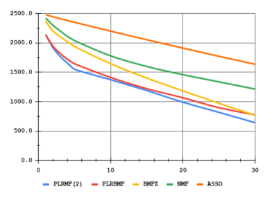
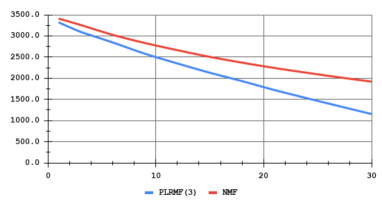
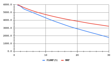
Figure 1: Graph on synthetic data where the entries in the table are average error on 10 random $50\times 100$ matrices.

3.1 Synthetic Data

We analyze our algorithms on binary matrices and compare with NMF, BMFZ, and Asso on random matrices of dimension $50\times 100$. We run all the algorithms 10 times and take the best results. The output of the NMF will be two factor matrices over reals. We compare the error of our algorithm with $||\mathbf{A}-\mathbf{U}\mathbf{V}||_{1}$, where $\mathbf{U}$ and $\mathbf{V}$ are the factors output by NMF on the input $\mathbf{A}$. The results are summarized in Tables 1. Even without rounding the factors of the output of NMF, our algorithms perform better. We would like to mention that NMF is designed to get factors with the objective of minimizing $||\mathbf{A}-\mathbf{U}\mathbf{V}||^{2}_{F}$. For our problem the error is measured in terms of $\ell_{1}$-norm and so we are getting better results than NMF. We also compare PLRMF($3$) and PLRMF($5$) with NMF. The performance of our algorithms are summarized in Figure 1. PLRMF(2) is giving $>15\%$ improvement over BMFZ for rank $3$ to $30$. PLRMF(5) percentage improvement over NMF is monotonously increasing: we have more than $3\%$ improvement on rank $3$, more than $11\%$ improvement on rank $12$, and more than $26\%$ improvement on rank $21$.

3.2 Experimental Results on Real-world Data

Table 2: Performance of our algorithm PLRBMF compared to NMF and BMFZ. The dimension of the image is $561\times 800$.

	NMF	BMFZ	PLRBMF
Original image
Rank: 10
	Error: 40213	Error: 37485	Error: 35034
Rank: 20
	Error: 37288	Error: 27180	Error: 23763
Rank: 30
	Error: 35938	Error: 21115	Error: 19081
Rank: 40
	Error: 34414	Error: 17502	Error: 15723
Rank: 50
	Error: 34445	Error: 14974	Error: 13684
Rank: 100
	Error: 33445	Error: 8709	Error: 8529

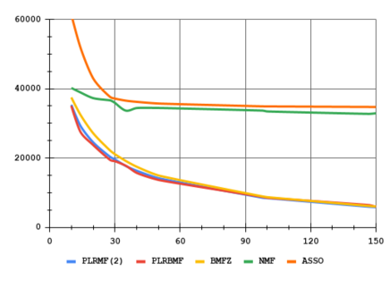
Figure 2: Graph depicting performance of our algorithms compared with others on the image mentioned in Table 2.

We analyse performance of our algorithms on binary and gray scale images. Table 2 shows the performance of PLRBMF compared with NMF and BMFZ. We would like to mention that both our algorithms PLRBMF and PLRMF($2$) work better than Asso, NMF, and BMFZ. Here, we included results of PLRBMF, NMF, and BMFZ. For the ranks mentioned in the table, PLRBMF performs better than PLRMF($2$) and both these algorithms perform better than the other algorithms mentioned here. For the inputs in Table 2, NMF and BMFZ perform better than Asso. So we compared PLRBMF with NMF and BMFZ. The performance of all the above algorithms are summarized in Figure 2. Notice that NMF gives two no-negative real matrices $\mathbf{U}$ and $\mathbf{V}$. We round the values in these matrices to $0$ and $1$ by choosing a best possible threshold that minimizes error in terms of $\ell_{1}$-norm. After rounding the values in the matrices $\mathbf{U}$ and $\mathbf{V}$ we get two binary matrices $\mathbf{U}^{\prime}$ and $\mathbf{V}^{\prime}$. Then we multiply $\mathbf{U}^{\prime}$ and $\mathbf{V}^{\prime}$ in GF(2) to get the output matrix.

In Table 3, we have taken an MRI Grayscale image, which consists of only 7 shades, as an input matrix whose dimensions are 266 $\times$ 247. This image is obtained by changing values between $0-255$ to $7$ distinct values of an image from [34]. For running PLRMF(7) on this image, we mapped those 7 shades to the numbers 0, 1, …, 6 so that we can get a matrix in GF(7), then we run PLRMF(7) on the modified matrix and again remapped the entries of output matrix to their respective shades, thereby, getting an output image and then we calculated error (sum of absolute errors) between input matrix and output matrix. For NMF we took the original matrix as the input (i.e., the matrix with values from $0-255$). Also, since NMF gives us a matrix with real values, we have rounded the matrix values to the nearest integer and called it the output matrix and then calculated error. We can see clearly from Table 3 and Figure 3 that PLRMF(7) which works only on finite fields is performing far better than NMF. It is important to note here that the input rank used in both the algorithms PLRMF(7) and NMF in Table 3 varies from 20 to 100. However, since the output of NMF algorithm is two real-valued factor matrices $\mathbf{U}$ and $\mathbf{V}$, and to get the output image the real values in $\mathbf{U}\mathbf{V}$ were rounded up to the nearest integer. Because of this, the rank of the output matrix is altered which is mentioned below the images in NMF column as Real Rank. Due to the increase in rank and the values in the output matrix of NMF can have much more than 7 distinct values, the images under the NMF column look better despite having higher error. To get the bounded rank output by the method of NMF, when we round the elements of the factor matrices to the nearest integer, the output matrix has all values zeros, resulting in a image with all pixels black.

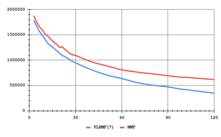
Figure 3: Graph depicting performance of our algorithm compared with NMF on the image mentioned in Table 3.

Table 3: Performance of our algorithm PLRMF(7) compared to NMF. The dimension of the image is $266\times 247$. Here Alg. Rank is the input parameter $r$ to the algorithms.

	PLRMF(7)	NMF
Original image
Alg. Rank: 10
	Error: 1419231	Error: 1523339
	GF(7) Rank : 10	Real Rank : 247
Alg. Rank: 20
	Error: 1129755	Error: 1248532
	GF(7) Rank : 20	Real Rank : 247
Alg. Rank: 30
	Error: 947298	Error: 1093683
	GF(7) Rank : 30	Real Rank : 247
Alg. Rank: 50
	Error: 709203	Error: 888976
	GF(7) Rank : 50	Real Rank : 247
Alg. Rank: 100
	Error: 424776	Error: 664537
	GF(7) Rank : 100	Real Rank : 247

Table 4: Comparison on movie-lens data where the ranks considered are between $1$ and $30$, on matrix of dimension $43\times 134$.

Rank	1	2	3	6
PLRMF($11$)	4981	4527	4273	3791
NMF	5257.8	5201	5015	4652.7

Rank	9	12	15	18
PLRMF($11$)	3422	3070	2935	2477
NMF	3924	3628	4305.6	4066.4

Rank	21	24	27	30
PLRMF($11$)	2145	1935	1569	1129
NMF	3556	3336	3090	2982

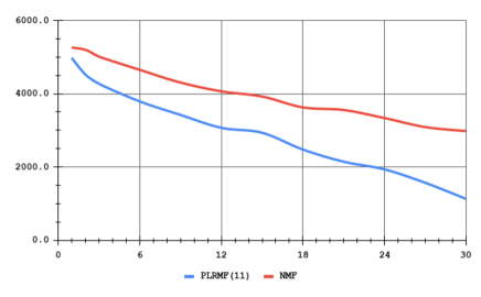
Figure 4: Graph on real data where the entries in the table are entries in user vs movie matrix of movie lens data set where each user has rated at least 200 movies and each movie is rated by at least 150 users. The dimension of the matrix is $43\times 134$.

We analyze PLRMF($11$) on movielens data set [35] and compare it with NMF and the performance can be found in Figure 4 and Table 4. The performance of PLRMF($11$) against NMF, monotonically increasing with respect to rank. We obtain more than $14\%$ improvement on rank $3$, more than $24\%$ improvement on rank $12$, and more than $39\%$ improvement on rank $21$ against NMF.

4 Conclusion

In this work we designed heuristic algorithms for BMF and $\mathbb{F}_{p}$-Matrix Factorization that are inspired by the theoretical algorithms for the same. Even though our algorithms have less error compared with the benchmark algorithms we considered, the later run faster as they are truely polynomial time algorithms. It is interesting research direction to improve the running time of the algorithm along with obtaining less error.

References

- [1] K. Pearson, “Liii. on lines and planes of closest fit to systems of points in space,” The London, Edinburgh, and Dublin Philosophical Magazine and Journal of Science, vol. 2, no. 11, pp. 559–572, 1901.
- [2] H. Hotelling, “Analysis of a complex of statistical variables into principal components.” Journal of educational psychology, vol. 24, no. 6, p. 417, 1933.
- [3] C. Eckart and G. Young, “The approximation of one matrix by another of lower rank,” Psychometrika, vol. 1, no. 3, pp. 211–218, 1936.
- [4] C. Spearman, “” general intelligence” objectively determined and measured.” 1961.
- [5] L. Mirsky, “Symmetric gauge functions and unitarily invariant norms,” Quart. J. Math. Oxford Ser. (2), vol. 11, pp. 50–59, 1960. [Online]. Available: https://doi.org/10.1093/qmath/11.1.50
- [6] P. Miettinen and S. Neumann, “Recent developments in boolean matrix factorization,” in Proceedings of the Twenty-Ninth International Joint Conference on Artificial Intelligence, IJCAI-20. International Joint Conferences on Artificial Intelligence Organization, 7 2020, pp. 4922–4928, survey track.
- [7] Y. Fu, N. Jiang, and H. Sun, “Binary matrix factorization and consensus algorithms,” in Proceedings of the International Conference on Electrical and Control Engineering (ICECE). IEEE, 2010, pp. 4563–4567.
- [8] B.-H. Shen, S. Ji, and J. Ye, “Mining discrete patterns via binary matrix factorization,” in Proceedings of the 15th ACM SIGKDD International Conference on Knowledge Discovery and Data Mining (KDD). New York, NY, USA: ACM, 2009, pp. 757–766. [Online]. Available: http://doi.acm.org/10.1145/1557019.1557103
- [9] P. Jiang, J. Peng, M. Heath, and R. Yang, “A clustering approach to constrained binary matrix factorization,” in Data Mining and Knowledge Discovery for Big Data: Methodologies, Challenge and Opportunities. Berlin, Heidelberg: Springer Berlin Heidelberg, 2014, pp. 281–303.
- [10] M. Koyutürk and A. Grama, “Proximus: A framework for analyzing very high dimensional discrete-attributed datasets,” in Proceedings of the 9th ACM SIGKDD International Conference on Knowledge Discovery and Data Mining (KDD). New York, NY, USA: ACM, 2003, pp. 147–156. [Online]. Available: http://doi.acm.org/10.1145/956750.956770
- [11] H. Lu, J. Vaidya, and V. Atluri, “Optimal boolean matrix decomposition: Application to role engineering,” in Proceedings of the 24th International Conference on Data Engineering, (ICDE), 2008, pp. 297–306. [Online]. Available: https://doi.org/10.1109/ICDE.2008.4497438
- [12] S. Hess, K. Morik, and N. Piatkowski, “The PRIMPING routine - tiling through proximal alternating linearized minimization,” Data Min. Knowl. Discov., vol. 31, no. 4, pp. 1090–1131, 2017. [Online]. Available: https://doi.org/10.1007/s10618-017-0508-z
- [13] F. Ban, V. Bhattiprolu, K. Bringmann, P. Kolev, E. Lee, and D. P. Woodruff, “A PTAS for p-low rank approximation,” in Proceedings of the Thirtieth Annual ACM-SIAM Symposium on Discrete Algorithms, SODA 2019, San Diego, California, USA, January 6-9, 2019. SIAM, 2019, pp. 747–766. [Online]. Available: https://doi.org/10.1137/1.9781611975482.47
- [14] F. V. Fomin, P. A. Golovach, D. Lokshtanov, F. Panolan, and S. Saurabh, “Approximation schemes for low-rank binary matrix approximation problems,” ACM Trans. Algorithms, vol. 16, no. 1, pp. 12:1–12:39, 2020. [Online]. Available: https://doi.org/10.1145/3365653
- [15] R. Kumar, R. Panigrahy, A. Rahimi, and D. P. Woodruff, “Faster algorithms for binary matrix factorization,” in Proceedings of the 36th International Conference on Machine Learning, ICML 2019, 9-15 June 2019, Long Beach, California, USA, ser. Proceedings of Machine Learning Research, vol. 97. PMLR, 2019, pp. 3551–3559.
- [16] P. Miettinen, T. Mielikäinen, A. Gionis, G. Das, and H. Mannila, “The discrete basis problem,” IEEE Trans. Knowl. Data Eng., vol. 20, no. 10, pp. 1348–1362, 2008. [Online]. Available: https://doi.org/10.1109/TKDE.2008.53
- [17] J. Vaidya, V. Atluri, and Q. Guo, “The role mining problem: finding a minimal descriptive set of roles,” in Proceedings of the 12th ACM Symposium on Access Control Models and (SACMAT), 2007, pp. 175–184. [Online]. Available: http://doi.acm.org/10.1145/1266840.1266870
- [18] H. Lu, J. Vaidya, V. Atluri, and Y. Hong, “Constraint-aware role mining via extended boolean matrix decomposition,” IEEE Trans. Dependable Sec. Comput., vol. 9, no. 5, pp. 655–669, 2012. [Online]. Available: https://doi.org/10.1109/TDSC.2012.21
- [19] B. Mitra, S. Sural, J. Vaidya, and V. Atluri, “A survey of role mining,” ACM Comput. Surv., vol. 48, no. 4, pp. 50:1–50:37, Feb. 2016. [Online]. Available: http://doi.acm.org/10.1145/2871148
- [20] H. W. Gutch, P. Gruber, A. Yeredor, and F. J. Theis, “ICA over finite fields - separability and algorithms,” Signal Processing, vol. 92, no. 8, pp. 1796–1808, 2012. [Online]. Available: https://doi.org/10.1016/j.sigpro.2011.10.003
- [21] A. Painsky, S. Rosset, and M. Feder, “Generalized independent component analysis over finite alphabets,” IEEE Trans. Information Theory, vol. 62, no. 2, pp. 1038–1053, 2016. [Online]. Available: https://doi.org/10.1109/TIT.2015.2510657
- [22] A. Yeredor, “Independent component analysis over Galois fields of prime order,” IEEE Trans. Information Theory, vol. 57, no. 8, pp. 5342–5359, 2011. [Online]. Available: https://doi.org/10.1109/TIT.2011.2145090
- [23] M. W. Berry, S. T. Dumais, and G. W. O’Brien, “Using linear algebra for intelligent information retrieval,” SIAM review, vol. 37, no. 4, pp. 573–595, 1995.
- [24] R. Belohlávek and V. Vychodil, “Discovery of optimal factors in binary data via a novel method of matrix decomposition,” J. Computer and System Sciences, vol. 76, no. 1, pp. 3–20, 2010. [Online]. Available: https://doi.org/10.1016/j.jcss.2009.05.002
- [25] C. Dan, K. A. Hansen, H. Jiang, L. Wang, and Y. Zhou, “On low rank approximation of binary matrices,” CoRR, vol. abs/1511.01699, 2015. [Online]. Available: http://arxiv.org/abs/1511.01699
- [26] P. Miettinen and J. Vreeken, “Model order selection for boolean matrix factorization,” in Proceedings of the 17th ACM SIGKDD International Conference on Knowledge Discovery and Data Mining (KDD). ACM, 2011, pp. 51–59. [Online]. Available: http://doi.acm.org/10.1145/2020408.2020424
- [27] J. Vaidya, “Boolean matrix decomposition problem: Theory, variations and applications to data engineering,” in Proceedings of the 28th IEEE International Conference on Data Engineering (ICDE). IEEE Computer Society, 2012, pp. 1222–1224. [Online]. Available: https://doi.org/10.1109/ICDE.2012.144
- [28] N. Gillis and S. A. Vavasis, “On the complexity of robust PCA and -norm low-rank matrix approximation,” CoRR, vol. abs/1509.09236, 2015. [Online]. Available: http://arxiv.org/abs/1509.09236
- [29] F. V. Fomin, P. A. Golovach, and F. Panolan, “Parameterized low-rank binary matrix approximation,” Data Min. Knowl. Discov., vol. 34, no. 2, pp. 478–532, 2020. [Online]. Available: https://doi.org/10.1007/s10618-019-00669-5
- [30] A. Bhattacharya, D. Goyal, R. Jaiswal, and A. Kumar, “Streaming PTAS for binary -low rank approximation,” CoRR, vol. abs/1909.11744, 2019. [Online]. Available: http://arxiv.org/abs/1909.11744
- [31] A. Kumar, Y. Sabharwal, and S. Sen, “Linear-time approximation schemes for clustering problems in any dimensions,” J. ACM, vol. 57, no. 2, pp. 5:1–5:32, 2010. [Online]. Available: http://doi.acm.org/10.1145/1667053.1667054
- [32] S. P. Lloyd, “Least squares quantization in PCM,” IEEE Trans. Inf. Theory, vol. 28, no. 2, pp. 129–136, 1982. [Online]. Available: https://doi.org/10.1109/TIT.1982.1056489
- [33] D. D. Lee and H. S. Seung, “Learning the parts of objects by nonnegative matrix factorization,” Nature, vol. 401, pp. 788–791, 1999.
- [34] E. Binz and W. Schempp, “A unitary parallel filter bank approach to magnetic resonance tomography,” vol. 517, 05 2000.
- [35] F. M. Harper and J. A. Konstan, “The movielens datasets: History and context,” ACM Trans. Interact. Intell. Syst., vol. 5, no. 4, Dec. 2015. [Online]. Available: https://doi.org/10.1145/2827872