Fast convergence rates for dose-response estimation

Abstract

We consider the problem of estimating a dose-response curve, both globally and locally at a point. Continuous treatments arise often in practice, e.g. in the form of time spent on an operation, distance traveled to a location or dosage of a drug. Letting $A$ denote a continuous treatment variable, the target of inference is the expected outcome if everyone in the population takes treatment level $A=a$. Under standard assumptions, the dose-response function takes the form of a partial mean. Building upon the recent literature on nonparametric regression with estimated outcomes, we study three different estimators. As a global method, we construct an empirical-risk-minimization-based estimator with an explicit characterization of second-order remainder terms. As a local method, we develop a two-stage, doubly-robust (DR) learner. Finally, we construct a $m^{\text{th}}$-order estimator based on the theory of higher-order influence functions. Under certain conditions, this higher order estimator achieves the fastest rate of convergence that we are aware of for this problem. However, the other two approaches are easier to implement using off-the-shelf software, since they are formulated as two-stage regression tasks. For each estimator, we provide an upper bound on the mean-square error and investigate its finite-sample performance in a simulation. Finally, we describe a flexible, nonparametric method to perform sensitivity analysis to the no-unmeasured-confounding assumption when the treatment is continuous.

Keywords: continuous treatments, efficient influence function, orthogonal learning, observational studies.

1 Introduction

1.1   Notation & setup

Continuous or multi-valued treatments occur often in practice; time, distance traveled, or dosage of a drug are common examples. We study the problem of estimating the effect of a continuous treatment $A\in\mathcal{A}\subset\mathbb{R}$ on an outcome $Y\in\mathcal{Y}\subset\mathbb{R}$. Within the potential outcomes framework [Rubin, 1974], this effect is defined as the expectation of the potential outcome $Y^{a}$, which is the outcome observed if the subject takes treatment level $A=a$. In other words, the estimand represents the average outcome if everyone in the population had taken treatment level $a$. Because $A$ is continuous, $\mathbb{E}(Y^{a})$ is a curve, often referred to as the dose-response function (DRF). Under standard assumptions (see e.g. Kennedy et al. [2017]), the DRF takes the form of a partial mean:

$$\theta(t)=\mathbb{E}\{\mathbb{E}(Y\mid A=t,X)\}=\int\mathbb{E}(Y\mid A=t,X=x)d\mathbb{P}(x)$$

where $X\in\mathcal{X}\subset\mathbb{R}^{d}$ denotes measured confounders. Let $Z=(Y,A,X)$ be distributed according to some distribution $\mathbb{P}$ with density $p$ with respect to the Lebesgue measure. The goal of this paper is to discuss new ways of estimating $\theta(a)$ using $n$ iid copies of $Z$, which yield strong error guarantees, under weaker conditions, and fast rates of convergence. To simplify the notation we define:

$$p(u)=\frac{d}{du}\mathbb{P}(U\leq u),\quad\pi(a\mid x)=\frac{p(a,x)}{p(x)},\quad\mu(a,x)=\mathbb{E}(Y\mid A=a,X=x),\quad w(a,x)=\frac{p(a)}{\pi(a\mid x)}$$

That is, $p(u)$ is the density of $U$ at $U=u$, $\mu(a,x)$ is the outcome regression, and $\pi(a\mid x)$ is the conditional density of $A$ given $X=x$. We will sometimes denote all the nuisance functions by $\eta=\{p(a),p(x),\mu(a,x),\pi(a\mid x)\}$. With this notation, we have

$$\theta(t)=\mathbb{E}\{\mu(t,X)\}=\mathbb{E}\left\{w(t,X)Y\mid A=t\right\}$$

For a kernel function $K(u)$, we let $K_{ht}(a)=h^{-1}K((a-t)/h)$. We use the notation $\mathbb{P}\{g(Z)\}=\int g(z)d\mathbb{P}(z)$ and $\mathbb{P}_{n}\{g(Z)\}=n^{-1}\sum_{i=1}^{n}g(Z_{i})$ to denote means (given $g$) and sample means. Further, we let $\lVert f\rVert^{2}=\int f^{2}(z)d\mathbb{P}(z)=\mathbb{P}\{f^{2}(Z)\}$ to denote the squared $L_{2}(\mathbb{P})$ norm.

Throughout the paper, we will rely on the following assumptions. Additional assumptions will be introduced as needed.

1. Positivity: $\pi(a\mid x)$ and its estimator $\widehat{\pi}(a\mid x)$ are bounded above and away from zero for all $a\in\mathcal{A}$ and $x\in\mathcal{X}$;

2. Boundedness: $Y$, $A$, $\widehat{\mu}(a,x)$ are uniformly bounded.

Notice that Positivity is enough to define $\theta(a)=\int\mu(a,x)d\mathbb{P}(x)$, but not enough to interpret $\theta(a)$ as the dose-response curve. To interpret $\theta(a)$ as the effect of $A$ on $Y$, one needs to impose additional causal assumptions such as $Y^{a}\perp\!\!\!\perp A\mid X$ and $A=a\implies Y^{a}=Y$, i.e., no unmeasured confounding and consistency (e.g. no interference). This paper is about estimating $\theta(a)$, regardless of its interpretation, and we refer to Kennedy et al. [2017] and reference therein for more details on identification.

Finally, our focus will be on estimation of the dose-response in nonparametric models where the dose-response itself and the nuisance functions possess varying degrees of smoothness. In particular, we will distinguish between the smoothness levels of the dose response $a\mapsto\theta(a)$, the conditional density of the treatment given the measured confounders $(a,x)\mapsto\pi(a\mid x)$, and the outcome regression $(a,x)\mapsto\mu(a,x)$. We will further refine this distinction when introducing the $m^{\text{th}}$-order estimator in the sense that we will consider models where $a\mapsto\mu(a,x)$, $x\mapsto\mu(a,x)$, $a\mapsto\pi(a\mid x)$ and $x\mapsto\pi(a\mid x)$ may have different smoothness levels. Note that it is reasonable to expect the smoothness of $a\mapsto\mu(a,x)$ to match that of $a\mapsto\theta(a)=\int\mu(a,x)d\mathbb{P}(x)$ in most applications.

1.2   Literature review

Crucially, because $A$ is continuous, the parameter $\theta(t)$ cannot be estimated at $\sqrt{n}$ rates in nonparametric models. Informally, in order to see this, notice that we can write $\theta(t)=\mathbb{E}\{w(t,X)Y\mid A=t\}$ and thus even if $w(t,X)Y$ was fully observed (e.g., in a randomized experiment), the best convergence rate attainable would be that of nonparametric regression. In fact, in order to compare the performances of different estimators, it is useful to establish the regimes where they behave like the oracle estimator that has access to $w(t,X)Y$ and can regress it on $A$.

Definition 1 (Oracle rate).

Given an iid sample $Z_{1},\ldots,Z_{n}$, let $\widetilde{\theta}(\cdot)$ be the (infeasible) estimator regressing $w(t,X)Y$ on $A$ and let $r_{n}$ be its error under some loss, e.g., the square loss at a point: $\mathbb{E}[\{\widetilde{\theta}(t)-\theta(t)\}^{2}]$. We refer to $r_{n}$ as the oracle rate.

In nonparametric models that admit slow rates of convergence, two commonly employed strategies are either 1) to specify a marginal structural model $\theta(t)=m(t;\beta)$ [Robins, 2000] or 2) to change the target of inference from $\theta(t)$ to a projection of $\theta(t)$ onto a finite-dimensional model $g(t;\beta)$. We refer to Neugebauer and van der Laan [2007] and Ai et al. [2018] for discussions of efficient estimation in the latter case.

Another approach for estimation of dose-responses is to impose some nonparametric, structural assumptions on the curve itself. For instance, if it is known that the treatment cannot harm the patients, one may impose a monotonicity assumption [Westling et al., 2020; Westling and Carone, 2020]. Yet another approach is to choose a candidate estimator of $\theta(a)$ that minimizes a good estimate of the risk. The key insight is that, while $\theta(a)$ is generally not estimable at $\sqrt{n}$-rates, the integrated risk of a candidate estimator is [Díaz and van der Laan, 2013; Van der Laan et al., 2003].

In the context of nonparametric estimation, Newey [1994] derives sufficient conditions under which a two-stage kernel estimator of $\theta(t)$ is asymptotically normal and unbiased. Their estimator is of the plug-in variety and takes the form $\widehat{\theta}(a)=n^{-1}\sum_{i=1}^{n}\widehat{\mu}(t,X_{i})$, where $\widehat{\mu}(t,x)$ is a kernel-smoothed estimate of $\mu(t,x)$ depending on some bandwidth $h$. To achieve $\sqrt{nh}$-consistency and asymptotic unbiasedness, $\widehat{\mu}(t,x)$ has to be undersmoothed; i.e., $h$ has to be chosen smaller than that minimizing the asymptotic mean-square-error of $\widehat{\mu}(t,x)$. Choosing the right amount of undersmoothing presents challenges in practice; see e.g., Section 5.7 in Wasserman [2006]. Starting from the estimator considered in Newey [1994], Flores [2007] develops plug-in-type estimators of the maximum of $\theta(a)$ and the value of $a$ at which the maximum is attained. Galvao and Wang [2015] study estimation and testing of continuous treatment effects in general settings using inverse-probability-weighted estimators. Singh et al. [2020] analyze plug-in-type estimators of general causal functions based on reproducing kernel methods.

There exists another representation of the DRF that plays an important role in developing efficient estimators:

$$\theta(a)=\mathbb{E}\{\varphi(Z)\mid A=a\},\text{ where }\varphi(Z)=w(A,X)\{Y-\mu(A,X)\}+\int\mu(A,x)d\mathbb{P}(x)$$

This representation motivates estimators that regress the pseudo-outcome $\varphi(Z)$ onto $A$. Because this pseudo-outcome depends on unknown nuisance functions, it needs to be estimated from the data; thus we refer to the regression of $\varphi(Z)$ on $A$ as a second-stage regression. The crucial point is that $\varphi(Z)$ is such that an estimated regression $\widehat{\mathbb{E}}_{n}\{\widehat{\varphi}(Z)\mid A=a\}$ can behave like the oracle $\widehat{\mathbb{E}}_{n}\{\varphi(Z)\mid A=a\}$ even when $\widehat{\varphi}(Z)$ converges to $\varphi(Z)$ at a rate that is slower than the convergence of $\widehat{\mathbb{E}}_{n}\{\varphi(Z)\mid A=a\}$ to $\theta(a)$. We conclude this section with a review of the use of this pseudo-outcome in the estimators proposed in Kennedy et al. [2017], Semenova and Chernozhukov [2017] and Colangelo and Lee [2020], as they are the ones most similar to the estimators considered in this article.

1.3   Review of existing doubly-robust estimators

In this section, we review a few estimation strategies that are doubly-robust and yield fast convergence rates in the sense that the upper bound on the risk is of the form: “oracle rate + second order, doubly-robust remainder terms,” and thus yield consistent estimators when either $w(a,x)$ or $\mu(a,x)$, but not necessarily both, are consistently estimated. This is analogous to the case of treatment effects defined by categorical treatments, whereby estimators based on influence functions are doubly-robust and enjoy second-order error terms.

The estimators proposed in Semenova and Chernozhukov [2017] and Kennedy et al. [2017] are based on regressing an estimate of $\varphi(Z)$ onto $A$. The quantity $\varphi(Z)$ has a doubly robust remainder error, or equivalently, satisfies a Neyman-orthogonality condition in the sense that, for $\eta=\{p(A),\pi(A\mid X),\mu(A,X)\}$:

$$\partial r\mathbb{E}\{\varphi(Z;\eta_{0}+r(\overline{\eta}-\eta))\mid A=a\}|_{r=0}=0\text{ for all }a,\overline{\eta}.$$

This implies that the loss $\{\varphi(Z;\eta)-\theta(A)\}^{2}$ is universally Neyman-orthogonal in the sense that

$$\partial r_{2}\partial r_{1}\mathbb{E}[\varphi(Z;\eta_{0}+r_{2}(\eta-\eta_{0}))-\theta(A)-r_{1}\{\theta(A)-\overline{\theta}(A)\}]^{2}|_{r_{1}=r_{2}=0}$$

$$=-2\int\partial r\mathbb{E}\{\varphi(Z;\eta_{0}+r(\eta-\eta_{0}))\mid A=a\}_{r=0}\{\theta(a)-\overline{\theta}(a)\}d\mathbb{P}(a)$$

$$=0$$

for any $\theta,\overline{\theta}$.

Constructing estimators satisfying Neyman-orthogonality conditions has a long history in Statistics, albeit under different names. For example, in functional estimation, and, in particular, estimation of average treatment effects, estimators that are “Neyman-orthogonal,” “bias-corrected,” “augmented-inverse-probability-weighted,” or, more generally, constructed according to the “double machine learning” framework are all based on first-order functional Taylor expansions, also known as von-Mises expansions [Kennedy, 2022]. In fact, underlying Neyman orthogonality is a first-order expansion of the target estimand $\psi(\mathbb{P})$, viewed as a function of the unknown distribution $\mathbb{P}$, around an estimator $\widehat{\mathbb{P}}$ of $\mathbb{P}$. If the derivative term, say $\psi^{{}^{\prime}}(\mathbb{P}-\widehat{\mathbb{P}};\widehat{\mathbb{P}})$, exists then the estimator consisting of the (estimated) derivative term plus the initial estimator $\psi(\widehat{\mathbb{P}})$ should exhibit second-order error rates. For smooth functionals, the derivative term can be written as $\psi^{{}^{\prime}}(\mathbb{P}-\widehat{\mathbb{P}};\widehat{\mathbb{P}})=\int\phi(z;\widehat{\mathbb{P}})d\mathbb{P}(z)$, where $\phi(z)$ is the influence function and is mean-zero. For more complex parameters, such as the dose-response curve, this representation is generally not possible. However, one may try to express the derivative as an integral with respect to the conditional distribution of the observations given, for example, the treatment.

Kennedy et al. [2017] show that, when the second stage regression $\widehat{\mathbb{E}}_{n}(\widehat{\varphi}(Z)\mid A=a)$ is a local linear regression, then the oracle rate (the rate achievable if $\varphi(Z)$ was fully observed as defined in Definition 1) is attained as long as

$$\sup_{a:|a-t|\leq h}\|\widehat{\pi}(a\mid X)-\pi(a\mid X)\|\|\widehat{\mu}(a,X)-\mu(a,X)\|=o_{\mathbb{P}}(1/\sqrt{nh}),$$ (1)

where $h$ is the bandwidth used in the second-stage regression. A similar requirement appears in Colangelo and Lee [2020]. Notice that this error term is second order, as it is a product of errors. It also reveals the double-robustness property of $\varphi(Z)$: consistency of $\widehat{\mathbb{E}}_{n}\{\widehat{\varphi}(Z)\mid A=a\}$ requires consistency of either $\pi(A\mid X)$ or $\mu(A,X)$ but not necessarily both.

Semenova and Chernozhukov [2017] studies an estimator of the same form $\mathbb{P}_{n}^{*}\{\widehat{\varphi}(Z)\mid A=a\}$ where $\mathbb{P}_{n}^{*}$ is a series estimator. Their estimator uses cross-fitting, whereby, for a given fold $k$, the nuisance functions are estimated on all folds but $k$, and $\mathbb{P}_{n}^{*}$ is computed using observations from $k$. This construction bypasses the need to impose Donsker conditions on the nuisance functions. We note that, relative to the results in Kennedy et al. [2017] and Colangelo and Lee [2020], those in Semenova and Chernozhukov [2017] appear to require that the product of root-mean-square-errors for estimating $\mu(a,x)$ and $\pi(a\mid x)$ is of smaller order than $1/\sqrt{nk}$, where $k$ is the dimension of the basis (Assumptions 3.5 and 4.9). This is more stringent of a requirement than (1).

The approach taken by Colangelo and Lee [2020] is different in that instead of regressing $\widehat{\varphi}(Z)$ onto $A$, the estimator is

$$\widehat{\theta}(t)=\frac{1}{n}\sum_{i=1}^{n}\left[\frac{K_{ht}(A_{i})\{Y_{i}-\widehat{\mu}(t,X_{i})\}}{\widehat{\pi}(t\mid X_{i})}+\widehat{\mu}(t,X_{i})\right]$$ (2)

They motivate their estimator as being based on an approximate first-order influence function, which can be calculated as the Gateaux derivative with respect to smooth deviations from the true data-generating distribution as these deviations approach a distribution with point-mass at $A=t$ (see their Section 4). This estimator still enjoys second order rates, but, it is not immediately clear how it adapts to different level of smoothness of $\theta(a)$. That is, their error rates may be of the form “oracle + second-order terms” only in certain smoothness regimes of $\theta(a)$. This is in contrast to estimators based on regressing $\widehat{\varphi}(Z)$ on $A$, which would behave like an oracle, and thus adapt to the smoothness of $\theta(a)$, as long as the second-order remainder terms are negligible. Their analysis focuses on low-smoothness regimes; viewed as a function of $a$, they assume that the joint density of the observations is three-times continuously differentiable. Notice that this implies that both the outcome regression $a\mapsto\mu(a,x)$ and the conditional density $a\mapsto\pi(a\mid x)$ are three-times continuously differentiable. In practice, however, it could be that $a\mapsto\mu(a,x)$ and thus the dose-response curve are smoother than $a\mapsto\pi(a\mid x)$. Our $m^{\text{th}}$-order estimator is an extension of (2) and appears to track the smoothness of the dose-response only in cases when this is no-greater than the smoothness of $a\mapsto\pi(a\mid x)$, which appears to be consistent with the results in Colangelo and Lee [2020].

1.4   Our contribution

Our contribution is mainly three-fold. We study three approaches to dose-response estimation: one based on estimators relying on approximate first-order influence functions and one based on higher-order corrections. For the first approach, we consider two estimation strategies. The first one is based on empirical loss minimization, which we view as a “global” method since it naturally estimates the curve on its entire support. Our approach specializes the results of Foster and Syrgkanis [2019] on empirical loss minimization with estimated outcomes to estimate dose-response functions under the square-loss. Importantly, we show that the resulting estimator is doubly-robust and give an explicit characterization of the remainder term. This, in turn, implies faster rates of convergence than those directly obtainable from the results in Foster and Syrgkanis [2019] whenever the treatment and the outcome models are estimated at different rates. The second one extends the DR-learner estimator of the conditional average treatment effect (proposed in Kennedy [2020]) to the continuous treatment effect setting. We view this as a “local” method since it estimates the dose-response at a specific point.

Next, we show how convergence rates can be substantially improved using kernel-smoothed, approximate higher order influence functions [Robins et al., 2008, 2009a, 2017]. To the best of our knowledge, our higher order estimator is the first use of higher order influence functions to estimate a dose-response curve. Further, we are not aware of other estimators of the dose-response curve that exhibit convergence rates as fast as that of our higher order estimator, under similar assumptions on the data generating process.

Finally, extending the work of Bonvini et al. [2022] on sensitivity analysis in marginal structural models, we describe a simple, yet flexible framework to gauge the impact of potential unmeasured confounders on the dose-response estimates. We analyze the performance of DR-Learner-based estimators of the bounds on the dose-response function derived under the sensitivity model.

2 Doubly-robust estimators

2.1   General doubly-robust estimation procedure

Here, we expand on the list of estimators enjoying second-order, doubly robust errors. We will show that extensions of the general procedure proposed in Foster and Syrgkanis [2019] and the DR-learner approach proposed by Kennedy [2020] in the context of conditional effects defined by binary treatments also yield estimators enjoying second-order and doubly-robust remainder terms. The work by Foster and Syrgkanis [2019] is rather general and already yields estimators that have second-order remainder terms, but their rates are in terms of $\lVert\widehat{\eta}-\eta\rVert_{\mathcal{F}}$ where $\lVert f\rVert_{\mathcal{F}}$ is a norm for the function spaces where all nuisance functions $\eta$ live in. We apply their results to the dose-response settings and show that it is possible to obtain estimators that are also doubly-robust. Establishing the double-robustness property, i.e. that the second order remainder term is a product of errors, is particularly important when the estimators of the nuisance functions converge at different rates, since the product of the errors would be of smaller order than the sum of the squared errors.

Let $Z_{1}^{n},Z_{2}^{n}$ and $Z_{3}^{n}$ denote three independent samples. We will work with estimates of the pseudo-outcome $\varphi(Z_{j})$ of the form

$$\widehat{\varphi}(Z_{j})=\widehat{w}(A_{j},X_{j})\{Y_{j}-\widehat{\mu}(A_{j},X_{j})\}+\frac{1}{n}\sum_{i=1}^{n}\widehat{\mu}(A_{j},X_{i})$$

where $\widehat{\mu}(a,x)$ and $\widehat{w}(a,x)$ are estimated using observations in $Z_{1}^{n}$, the observations $(X_{i})_{i=1}^{n}$ belong to $Z_{2}^{n}$ and $Z_{j}$ belongs to $Z_{3}^{n}$. An alternative approach, taken in Semenova and Chernozhukov [2017], is to consider only two samples, say $Z_{1}^{n}$ and $Z_{2}^{n}$, and compute

$$\widehat{\varphi}(Z_{j})=\widehat{w}(A_{j},X_{j})\{Y_{j}-\widehat{\mu}(A_{j},X_{j})\}+\frac{1}{n}\sum_{i\neq j}^{n}\widehat{\mu}(A_{j},X_{i})$$

for $Z_{j}$ and $(X_{i})_{i=1}^{n}$ in the same sample $Z_{2}^{n}$. We proceed by considering three separate samples to simplify the analysis of all our estimators, as we have $\widehat{\varphi}(Z_{k})\perp\!\!\!\perp\widehat{\varphi}(Z_{l})\mid(Z_{1}^{n},Z_{2}^{n})$ for $k\neq l$. The roles of $Z_{1}^{n}$, $Z_{2}^{n}$ and $Z_{3}^{n}$ can be swapped, which results in three estimators of $\theta(t)$. One can then take their average as the final estimator. From a sample of iid observations, it is possible to obtain separate independent samples simply by randomly split the data into sub-samples. To keep the notation as light as possible, we analyze the theoretical properties of the estimators based a single split into three subsamples. However, we expect the same arguments to hold when multiple splits are performed.

Our estimation procedure is summarized in the following algorithm.

Algorithm 1.

Let $Z_{1}^{n}$, $Z_{2}^{n}$ and $Z_{3}^{n}$ denote three independent samples of $n$ iid observations of $Z=(Y,A,X)$.

1. Nuisance training

   • Using only observations in $Z_{1}^{n}$, estimate $\mu(A,X)$ with $\widehat{\mu}(A,X)$ and $w(A,X)$ with $\widehat{w}(A,X)$;

   • Using only observations in $Z_{2}^{n}$, estimate $m(a)=\int\mu(a,x)p(x)dx$ with $\widehat{m}(a)=n^{-1}\sum_{i=1}^{n}\widehat{\mu}(a,X_{i})$.

2. Pseudo-outcome construction: using observations in $Z_{3}^{n}$, construct the pseudo-outcome

   $$\widehat{\varphi}(Z)=\widehat{w}(A,X)\{Y-\widehat{\mu}(A,X)\}+\widehat{m}(A)$$

3. Second stage regression, either of the following:

   • Empirical-risk-minimization: Define $\widehat{\theta}$ to be the empirical risk minimizer

     $$\widehat{\theta}=\operatorname*{arg\,min}_{\theta\in\Theta}\frac{1}{n}\sum_{i\in Z_{3}^{n}}\{\widehat{\varphi}(Z_{i})-\theta(A_{i})\}^{2}$$

     where $\Theta$ is some function class.

   • DR-Learner: Define

     $$\widehat{\theta}(t)=\frac{1}{n}\sum_{i\in Z_{3}^{n}}W_{i}(t;A^{n})\widehat{\varphi}(Z_{i})$$

     where $W_{i}(t;A^{n})$ are weights depending on $t$ and $A^{n}=(A_{1},\ldots,A_{n})\subset Z_{3}^{n}$.

4. (Optional) Cross-fitting: swap the role of $Z_{1}^{n}$, $Z_{2}^{n}$ and $Z_{3}^{n}$ and repeat steps 1 and 2. Use the average of the three estimators as an estimate of $\theta$.

In the following two sections, we give error bounds for a procedure that generalizes Algorithm 1. In particular, the bounds apply to the problem of estimating some $\theta(u)\equiv\mathbb{E}\{f(Z)\mid U=u\}$, where $U$ is some observed subset of $Z$ and $f(Z)$ is not directly observable. The estimator is $\widehat{\theta}(u)=\widehat{\mathbb{E}}_{n}\{\widehat{f}(Z)\mid U=u\}$, where $\widehat{\mathbb{E}}_{n}(\cdot\mid U=u)$ is either an empirical risk minimizer or a linear smoother and it is computed from a sample independent of that used to construct $\widehat{f}(\cdot)$. One can see that Algorithm 1 fits exactly this framework where $f(Z)=\varphi(Z)$. The additional sample split considered in Algorithm 1 is not needed to derive the next two propositions but it is useful to derive the result in Lemma 1. Finally, both bounds on the risk will involve a particular bias term $\widehat{r}(u)$ that would need to be analyzed on a case-by-case basis

$$\widehat{r}(u)=\int\widehat{f}(z)d\mathbb{P}(z\mid U=u)-\theta_{0}(u).$$

To estimate a dose-response curve, we have $f(Z)=\varphi(Z)$ and we propose using $\widehat{\varphi}(Z)$ as an estimator of $\varphi(Z)$, as detailed in Algorithm 1. Lemma 1 below shows that $\widehat{r}(u)$ is second-order and doubly-robust.

2.2   Upper bound on the risk of the ERM-based estimator

We start by considering estimating $\theta(t)$ via empirical loss minimization as in Algorithm 1 (a). We view this as a “global” method, as we estimate the function on its entire support as opposed to local methods, such as the DR-Learner discussed next, whereby the dose-response is estimated at a specific point. The error bound we describe in this section will be on the $L_{2}$ loss and will be a specialization of the results described in Foster and Syrgkanis [2019] and Wainwright [2019]. Foster and Syrgkanis [2019] provides a general framework for doing empirical risk minimization in the presence of nuisance components that need to be estimated. Here, we take their approach and find that the oracle rate is achievable if $\mathbb{E}\|\widehat{r}\|^{2}$ is simply of smaller order. In particular, from Lemma 3, if the orthogonal signal $\varphi(Z)$ is used, $\widehat{r}$ consists of a product of errors, as opposed to simply being of second order, and thus the bound on the MSE of our procedure improves upon the bound from Foster and Syrgkanis [2019].

The next proposition provides a bound on the error incurred by an estimator that uses an estimated outcome $\widehat{f}(Z)$ in place of the true (unobservable) outcome $f(Z)$, when doing empirical risk minimization with the square loss to estimate a regression function $\mathbb{E}\{f(Z)\mid U=u\}$.

Proposition 1.

Consider two independent samples, $D^{n}=(Z_{01},\ldots,Z_{0n})$ and $Z^{n}=(Z_{1},\ldots,Z_{n})$, consisting of $n$ iid copies of some generic observation $Z$ distributed according to $\mathbb{P}$. Let $U$ denote a generic variable such that $U\subset Z$. Let $\theta_{0}(u)\equiv\mathbb{E}\{f(Z)\mid U=u\}$ and suppose $\widehat{f}(\cdot)$ is constructed using only observations in $D^{n}$. Consider the estimator

$$\widehat{\theta}\equiv\operatorname*{arg\,min}_{\theta\in\Theta}\frac{1}{n}\sum_{i=1}^{n}\{\widehat{f}(Z_{i})-\theta(U_{i})\}^{2}.$$

Let $\theta^{*}=\operatorname*{arg\,min}_{\theta\in\Theta}\lVert\theta-\theta_{0}\rVert$ and $\Theta^{*}=\{\theta-\theta^{*}:\theta\in\Theta\}$. Define the local Rademacher complexity:

$$\mathcal{R}_{n}(\Theta^{*},\delta)=\mathbb{E}\left\{\sup_{g\in\Theta^{*}:\|g\|\leq\delta}\left|\frac{1}{n}\sum_{i=1}^{n}\epsilon_{i}g(U_{i})\right|\right\}$$

where $\epsilon_{1},\ldots,\epsilon_{n}$ are iid Rademacher random variables, independent of the sample. Suppose $\Theta^{*}$ is star-shaped and $S\equiv\sup_{z\in\mathcal{Z}}|\widehat{f}(z)|\ \lor\sup_{\theta\in\Theta}\|\theta\|_{\infty}$ is finite. Let $\delta_{n}$ be any solution to $\mathcal{R}_{n}(\Theta^{*},\delta)\leq\delta^{2}$ that satisfies

$$\delta_{n}^{2}\gtrsim\frac{\log\log(n)}{n}\lor\frac{1}{2n}.$$

Then,

$$\mathbb{E}(\lVert\widehat{\theta}-\theta_{0}\rVert^{2})\lesssim\lVert\theta^{*}-\theta_{0}\rVert^{2}+\delta_{n}^{2}+\mathbb{E}(\lVert\widehat{r}\rVert^{2})$$

where $\lVert f\rVert^{2}=\int f^{2}(z)d\mathbb{P}(z)$.

The error bound from Proposition 1 takes the form of an oracle rate plus a term involving $\widehat{r}$, which is controlled by Lemma 1 when $f(Z)=\varphi(Z)$ and $\widehat{f}(Z)=\widehat{\varphi}(Z)$.

The assumptions underlying Theorem 1 are rather mild. Appendix D in Foster and Syrgkanis [2019] and Chapters 13 and 14 in Wainwright [2019] describe common classes of functions for which the theorem applies, e.g., linear functions with constraints on the coefficients, functions satisfying Sobolev-type constraints or Reproducing Kernel Hilbert spaces. In order to apply Proposition 1, the class of functions considered has to be star-shaped. A class is star-shaped around the origin if, for any $g\in\mathcal{G}$ and $\alpha\in[0,1]$, it is the case that $\alpha g\in\mathcal{G}$. Importantly, a convex set is star-shaped. If the star-shaped condition is not met, the statement of the theorem would hold for $\delta_{n}$ defined in terms of the star-hull of the function class. The boundedness assumption on $\widehat{\varphi}(Z)$ and $\Theta$ is used in various places in the proof, including in ensuring that the square-loss is globally Lipschitz; we expect this assumption to hold when the observations are bounded. Finally, the inequality involving $\delta_{n}$ should often be satisfied. For instance, $\delta^{2}_{n}\geq 1/(2n)$ as long as $\Theta^{*}$ contains the constant function $\theta(u)=1$.

Example 1 (Orthogonal series, Examples 13.14 and 13.15 in Wainwright [2019]).

Suppose $\theta(u)$ is $\alpha$-times differentiable with $\theta^{(\alpha)}(u)$ satisfying $\int\{\theta^{(\alpha)}(u)\}^{2}d\mathbb{P}(u)\leq B$ for some constant $B$. Let $\{p_{j}\}_{j=1}^{\infty}$ be an orthonormal basis of $L_{2}(\mathbb{P})$, such as the sine / cosine basis (see Belloni et al. [2015] for a discussion on different basis choices). Consider estimating $\theta_{0}$ via ERM over the function class

$$\Theta(k,b)=\left\{\theta_{c}(\cdot):\sum_{j=1}^{k}p_{j}(\cdot)c_{j},\ \sum_{j=1}^{k}c_{j}^{2}\leq 1,\text{ and }|\theta_{c}(\cdot)|\ \leq b\right\}$$

Writing $\theta_{0}(u)=\sum_{j=1}^{\infty}p_{j}(u)c_{0j}$, we have $\theta^{*}(u)=\sum_{j=1}^{k}p_{j}(u)c_{0j}$ and $\lVert\theta^{*}-\theta_{0}\rVert^{2}=\sum_{j=k+1}^{\infty}c_{0j}^{2}$. It can be shown that $\lVert\theta^{*}-\theta_{0}\rVert^{2}\leq k^{-2\alpha}$. Furthermore, the function class $\Theta^{*}(k)=\{\theta-\theta^{*},\theta\in\Theta(k)\}=\Theta(k,2b)$ is convex and thus star-shaped and can be shown to satisfy $\delta^{2}_{n}\lesssim k/n$. Thus, Proposition 1 provides an upper bound of the mean-square error of the order

$$\mathbb{E}(\lVert\widehat{\theta}-\theta\rVert^{2})\lesssim k^{-2\alpha}+\frac{k}{n}+\mathbb{E}(\lVert\widehat{r}\rVert^{2})$$

If $k$ is chosen optimally, i.e. $k\sim n^{1/(2\alpha+1)}$, Proposition 1 shows that the oracle rate is attained as long as $\mathbb{E}(\lVert\widehat{r}\rVert^{2})$ is of order $O(n^{-2\alpha/(2\alpha+1)})$.

2.3   Upper bound on the risk of the linear smoothing-based estimator

In this section, we consider a DR-Learner-style estimator (cf. Van der Laan [2006] and Kennedy [2020] for heterogeneous effects of binary treatments). The DR-Learning framework proposed and analyzed in Kennedy [2020] covers a broad class of second-stage estimators satisfying a stability condition, linear smoothers being one example. Here, for simplicity, we consider the case where the second-stage estimator in $\widehat{\theta}(t)$ is based on localized linear smoothing. As discussed in Example 2, regressing $\widehat{\varphi}(Z)$ on $A$ via local polynomial regression represents an archetype of a localized DR-Learner. Kennedy et al. [2017] propose using generic learners to regress the estimated pseudo-outcome $\widehat{\varphi}(Z)$ on $A$ but only analyze local linear estimators. Thus, our next proposition is an extension to their work, in the spirit of analyzing more general linear smoothers. Theorem 1 and Proposition 1 in Kennedy [2020] yield the following proposition.

Proposition 2.

Consider two independent samples, $D^{n}=(Z_{01},\ldots,Z_{0n})$ and $Z^{n}=(Z_{1},\ldots,Z_{n})$, consisting of $n$ iid copies of some generic observation $Z$ distributed according to $\mathbb{P}$. Let $U$ denote a generic variable such that $U\subset Z$. Let $\theta_{0}(u)\equiv\mathbb{E}\{f(Z)\mid U=u\}$ and suppose $\widehat{f}(\cdot)$ is constructed using only observations in $D^{n}$. Consider the following estimator:

$$\widehat{\theta}(t)=n^{-1}\sum_{i=1}^{n}W_{i}(t;A^{n})\widehat{f}(Z)$$

Further suppose that the following regularity conditions hold:

• Minimum variance: $\text{var}\{f(Z)\mid U=u\}\geq c>0$ for all $u\in\mathcal{U}$ and some constant $c$;

• Consistency of nuisance estimators: $\sup_{z}|\widehat{f}(z)-f(z)|=o_{\mathbb{P}}(1)$;

• Localized weights: $n^{-1}\sum_{i=1}^{n}|W_{i}|\ \leq C$, for some constant $C$, and there exists a neighborhood $N_{t}$ around $U=t$ such that $W_{i}(t;U^{n})=0$ if $U_{i}\not\in N_{t}$.

Then, letting $\widetilde{\theta}(t)=n^{-1}\sum_{i=1}^{n}W_{i}(t;U^{n})f(Z_{i})$ denote the oracle estimator:

$$|\widehat{\theta}(t)-\theta_{0}(t)| \leq\left|\widetilde{\theta}(t)-\theta_{0}(t)\right|+\sup_{u\in N_{t}}\left|\widehat{r}(u)\right|+o_{\mathbb{P}}\left(\mathbb{E}\left[\left\{\widetilde{\theta}(t)-\theta_{0}(t)\right\}^{2}\right]\right).$$

As discussed in Kennedy [2020], the assumptions underlying Proposition 2 are easily satisfied for linear smoothers of the local polynomial regression variety. In particular, the weights of the local polynomial regression satisfies the assumptions (Tsybakov [2008], Lemma 1.3). This proposition follows from the results contained in Kennedy [2020] that apply to general linear smoothers, e.g. it does not require the weights to be localized. We work with localized weights to simplify the analysis of the point-wise risk.

Example 2.

Suppose $\theta_{0}(t)\equiv\mathbb{E}\{f(Z)\mid A=t\}$ belongs to a Hölder class of order $\alpha$ and let $p=\lfloor\alpha\rfloor$. A DR-Learner can be based upon local polynomial regression of order $p$. The weights are

$$W_{i}(t;A^{n})=s(t)^{T}\widehat{Q}^{-1}K_{ht}(A_{i})s(A_{i})^{T},$$

where $K(\cdot)$ is a kernel function, $\widehat{Q}=\mathbb{P}_{n}\{s(A)s(A)^{T}\}$ and $s(a)=\begin{bmatrix}1&\frac{a-t}{h}&\ldots&\left(\frac{a-t}{h}\right)^{p}\end{bmatrix}^{T}$. A standard calculation (see, for example, Tsybakov [2008]), yields that

$$\mathbb{E}\left[\left\{\widetilde{\theta}(t)-\theta_{0}(t)\right\}^{2}\right]=O(n^{-2\alpha/(2\alpha+1)})$$

This means that the oracle rate is attainable if $\sup_{u\in N_{t}}\widehat{r}^{2}(u)=O_{\mathbb{P}}(n^{-2\alpha/(2\alpha+1)})$, which is essentially the same requirement as for the estimator based on empirical-risk-minimization, see Example 1.

Remark 1.

From the bound in Proposition 2, inference can be carried out in the oracle regime, i.e., under the assumption that $\sup_{u\in N_{t}}|\widehat{r}(u)|$ is of smaller order that $|\widetilde{\theta}(t)-\theta(t)|$. In particular, if this holds, all inference tools for standard local nonparametric regression can be used. For example, let the setup be as in Example 2. Let $\sigma^{2}(t)$ be asymptotic variance of $\widetilde{\theta}(t)$, $\widehat{\sigma}^{2}(t)$ its consistent estimator and $b(t)$ the asymptotic bias. Then, if $\sup_{u\in N_{t}}\widehat{r}^{2}(u)=o_{\mathbb{P}}((nh)^{-1/2})$, we have

$$\frac{\sqrt{nh}[\widehat{\theta}(t)-\theta(t)-b(t)]}{\widehat{\sigma}(t)}\rightsquigarrow N(0,1)$$

as shown, for instance, in Section 4 of Fan and Gijbels [2018]. Notice that, without undersmoothing or bias-correction, a Wald-type confidence interval based on the asymptotic statement above will cover the smoothed dose-response curve $\mathbb{E}\{\widetilde{\theta}(t)\}$, rather than $\theta(t)$ itself (see Section 5.7 in Wasserman [2006] for more discussion).

2.4   Bounding the conditional bias of $\widehat{\varphi}(Z)$

As outlined in Propositions 1 and 2, the analysis of the estimator based on empirical risk minimization and that of the one based on linear smoothing yield a bound on the MSE that is the oracle rate plus a term of the order of $\widehat{r}^{2}(t)$. We show that $\widehat{r}(t)$ for $\widehat{f}(Z)=\widehat{\varphi}(Z)$ is second-order, as outlined in the following lemma.

Lemma 1.

Let $\widehat{r}(t)=\mathbb{E}\{\widehat{\varphi}(Z)\mid A=t,D^{n}\}-\theta_{0}(t)$. It holds that

$$|\widehat{r}(t)|\ \lesssim\lVert w-\widehat{w}\rVert_{t}\lVert\mu-\widehat{\mu}\rVert_{t}+\left|(\mathbb{P}_{n}-\mathbb{P})\{\widehat{\mu}(t,X)\}\right|$$

where $\lVert f\rVert^{2}_{t}=\int f^{2}(z)d\mathbb{P}(z\mid A=t)$ and $\mathbb{P}_{n}$ denotes an average over observations in sample $Z_{2}^{n}$.

Proof.

Recall that $\theta_{0}(t)=\mathbb{E}\{\varphi(Z)\mid A=t\}$. By Bayes’ rule, we have

$$\mathbb{P}\{\widehat{\mu}(t,X)\}-\theta(t)=\int w(t,x)\{\widehat{\mu}(t,x)-\mu(t,x)\}d\mathbb{P}(x\mid A=t)$$

and

$$\mathbb{E}\{\widehat{\varphi}(Z)\mid A=t,D^{n}\}=\int\widehat{w}(t,x)\{\mu(t,x)-\widehat{\mu}(t,x)\}d\mathbb{P}(x\mid A=t)+\mathbb{P}_{n}\{\widehat{\mu}(t,X)\}$$

Adding and subtracting $\mathbb{P}\{\widehat{\mu}(t,X)\}$ and applying Cauchy-Schwarz yield the result. ∎

The result from Lemma 1 shows that $|\widehat{r}(t)|$ can be bounded by the product of the $L_{2}$ errors in estimating $w(a,x)$ and $\mu(a,x)$ plus a centered sample average, which would generally be of the smaller order $O_{\mathbb{P}}(n^{-1/2})$ if, for instance, the second moment of $\widehat{\mu}(t,X)$ (conditional on $Z_{1}^{n}$) is bounded. In this respect, this term is effectively asymptotically negligible in nonparametric models where the rate of convergence is of slower order than $n^{-1/2}$. Thus, the conditional bias of $\widehat{\varphi}(Z)$ is driven by the product of the errors incurred in estimating the nuisance functions; this product structure of the bias is important when the nuisance functions are estimated at different rates.

Standard results are generally calculated for $L_{2}(d\mathbb{P}(a,x))$ errors defined by the joint distribution of $(A,X)$, for example

$$\lVert w-\widehat{w}\rVert^{2}\equiv\int\{w(a,x)-\widehat{w}(a,x)\}^{2}d\mathbb{P}(a,x).$$

In this case, optimal convergence rates for estimating $\mu(a,x)$ are well-understood for many classes. For instance, if $\mu(a,x)$ belongs to a Hölder class of order $\gamma$, then minimax-optimal convergence rates in $L_{2}(d\mathbb{P}(a,x))$ are of order $n^{-2\gamma/(2\gamma+d+1)}$. The bound from Lemma 1 is actually on an $L_{2}$ error with weight given by the conditional density of $X$ given $A=t$. In most settings, we expect the more conventional rate based on $L_{2}(d\mathbb{P}(a,x))$ to match that based on $L_{2}(d\mathbb{P}(x\mid A=t))$. For example, Result 1 from Colangelo and Lee [2020] shows that the rate in $L_{2}(d\mathbb{P}(x\mid A=t)p(t))$ matches that for the point-wise risk (in $(A,X)$) under a mild boundeness assumption. Alternatively, we note that one can always upper bound (up to constants) $\lVert f\rVert_{t}$ by the supremum norm $\lVert f\rVert_{\infty}$ and the rate for estimating a regression function in $L_{\infty}$ generally matches that for estimating the function in $L_{2}(d\mathbb{P}(a,x))$ up to log factors.

There are fewer results available for conditional density estimation compared to regression estimation. Recently Ai et al. [2018] have proposed a method to estimate $w(a,x)$ directly that, under certain conditions, exhibits a convergence rate in $L_{2}$ of order $n^{-2\gamma/(2\gamma+d+1)}$ if $w(a,x)$ is $\gamma$-smooth (see their Theorem 3). Alternatively, one can estimate $p(a)$ and $\pi(a\mid x)$ and compute their ratio to estimate $w(a,x)$. We refer to Colangelo and Lee [2020] for a discussion on ways to estimate $\pi(t\mid x)$. In particular, one approach is to estimate $\mathbb{E}\{G_{h_{1}t}(A)\mid X=x\}$, where $G(u)$ is some kernel and $h_{1}$ some bandwidth of choice. As a third approach, because $w(a,x)=p(a)p(x)/p(a,x)$, one can estimate the marginals $p(x)$ and $p(a)$ and the joint density $p(a,x)$ and take the ratio as an estimate of $w(a,x)$. Estimating a joint density of $d$ variables that belongs to a Hölder-class of order $\gamma$ can be done with error scaling as $n^{-2\gamma/(2\gamma+d)}$. Thus, the MSE of this ratio would trivially be upper bounded by the MSEs for estimating $p(a,x)$, $p(x)$ and $p(x)$, which would depend on their respective smoothness levels.

As investigated in more detail in the next section, an interesting setting is where $a\mapsto\mu(a,x)$ has a different smoothness level than $x\mapsto\mu(a,x)$, where we expect the former to match the smoothness of the dose-response $\theta(a)$ in many applications. This is an example of anisotropic regression. The optimal rate for estimating a $d$-dimensional regression in a Hölder class where each coordinate has its own level of smoothness $\gamma_{j}$ is of order $n^{-2\gamma/(1+2\gamma)}$, where $\gamma$ satisfies $\gamma^{-1}=\sum_{j=1}^{d}\gamma_{j}^{-1}$ [Hoffman and Lepski, 2002; Bertin, 2004]. If $\mu(a,x)$ is in an anisotropic Hölder class of order $(\alpha,b,\ldots,b)$, the rate simplifies to $n^{-2b/(2b+b/\alpha+d)}$, where $d=\dim(X)$. If the treatment $A$ is categorical or $\alpha$ is much larger than $b$, the rate is essentially $n^{-2b/(2b+d)}$, i.e. the optimal rate for estimating a $d$-dimensional regression function that is $b$-smooth. In a similar fashion, we may think of $a\mapsto\pi(a\mid x)$ and $x\mapsto\pi(a\mid x)$ as having different smoothness levels; optimal convergence rates in this context typically depend too on the harmonic means of the smoothness levels of each coordinate [Efromovich, 2007].

Remark 2.

Suppose the dose-response $\theta(a)$ belongs to a Hölder class of order $\alpha$ and that $w$ and $\mu$ are $s$-smooth so that they can be estimated in $L_{2}$ at the rate $n^{-2s/(2s+d+1)}$. Estimators whose risk is of the form “oracle rate + a term of the same order as $\widehat{r}$” would behave like an oracle estimator that has access to the true nuisance functions as soon as $s\geq(d+1)/\{2(1+1/\alpha)\}$. We will show that this oracle efficiency bar can be lowered, under certain conditions, by a higher order estimator. See Remark 7.

Remark 3.

We note that our discussion on the rates attained by the doubly-robust estimators discussed in Section 2 is driven by the bound computed in Lemma 1. If $\widehat{\mu}$ and $\widehat{w}$ are designed to optimally estimate $\mu$ and $w$, e.g. by selecting tuning parameters to minimize estimates of their MSEs, then generally the bound based on Cauchy-Schwarz is the best available. However, there are other techniques, such as particular forms of sample splitting coupled with undersmoothing, whereby the nuisance functions are estimated optimally with respect to the target of inference, and so the selected tuning parameters for the nuisance estimators may not minimize the MSEs with respect to the nuisance functions. This approach has favorable theoretical properties, see e.g. Kennedy [2020], although it can be challenging to implement in practice. We leave studying undersmoothing in the context of continuous treatments for future work.

Remark 4.

Compared to Theorem 2 in Kennedy et al. [2017], Theorem 2 and Lemma 1 provide the same error bound, but under substantially weaker conditions. Sample-splitting circumvents the need to impose Donsker-type conditions on the nuisance functions’ classes in the form of bounded uniform entropy integrals. Moreover, the use of local polynomial regression allows the estimator to track the smoothness of $\theta(a)$, thereby achieving the oracle rate in high smoothness regimes (provided that the remainder term is negligible).

3 Higher-order estimators

3.1   Preliminaries

Inspired by the seminal work of Robins et al. [2008, 2009a, 2017], in this section we investigate the use of higher-order influence functions (HOIFs) to estimate continuous treatment effects. To the best of our knowledge, this is the first time HOIFs are used in this context. For an introduction to higher-order influence functions, we refer to the main papers [Robins et al., 2009a, 2017] and give a brief overview here. Informally, an $m^{\text{th}}$-order estimator of a functional $\chi(p)$ (where $p$ is the density of the observations) takes the form

$$\widehat{\chi}(p)=\chi(\widehat{p})+\sum_{j=1}^{m}\mathbb{U}_{n}\{\widehat{\varphi}_{j}(Z_{1},\ldots,Z_{j})\}$$ (3)

where $\mathbb{U}_{n}$ is the $U$-statistic measure so that

$$\mathbb{U}_{n}\{\varphi_{j}(Z_{1},\ldots,Z_{j})\}=\frac{1}{n(n-1)\cdots(n-j+1)}\sum_{1\leq i_{1}\neq i_{2}\ldots\neq i_{j}\leq n}\varphi_{j}(Z_{i1},\ldots,Z_{ij}).$$

Letting $\mathbb{P}^{j}\{f(Z_{1},\ldots,Z_{j})\}=\int f(z_{1},\ldots,z_{j})d\mathbb{P}(z_{1})\ldots d\mathbb{P}(z_{j})$ denote the corresponding population measure, this implies an expansion:

$$\widehat{\chi}(p)-\chi(p)=\chi(\widehat{p})-\chi(p)+\sum_{j=1}^{m}\mathbb{P}^{j}\{\widehat{\varphi}_{j}(Z_{1},\ldots,Z_{j})\}+\sum_{j=1}^{m}(\mathbb{U}_{n}-\mathbb{P}^{j})\{\widehat{\varphi}_{j}(Z_{1},\ldots,Z_{j})\}$$

Following Robins et al. [2009a], van der Vaart [2014], Robins et al. [2017], if $\varphi_{j}$ is chosen such that $-\mathbb{P}^{j}\{\widehat{\varphi}_{j}(Z_{1},\ldots,Z_{j})\}$ acts as the $j^{\text{th}}$-order term in the functional Taylor expansion of $\chi(\widehat{p})-\chi(p)$, then

$$\chi(\widehat{p})-\chi(p)+\sum_{j=1}^{m}\mathbb{P}^{j}\{\widehat{\varphi}_{j}(Z_{1},\ldots,Z_{j})\}=O(d(p-\widehat{p})^{m+1})$$

for some distance $d(\cdot)$. The quantity $\varphi_{j}$ is referred to as the $j^{\text{th}}$-order influence function of $\chi(p)$. Provided that

$$\text{var}\left[\sum_{j=1}^{m}(\mathbb{U}_{n}-\mathbb{P}^{j})\{\widehat{\varphi}_{j}(Z_{1},\ldots,Z_{j})\}\right]=O(n^{-1}),$$

this calculation would suggest that $\widehat{\chi}(p)$ would always be root-$n$ consistent if $m$ is large enough. However, higher order influence functions do not exist for many functionals of interest, including the average treatment effect of a binary treatment. In our setting, the dose-response does not possess influence functions of any order, in nonparametric models. While this means that generally it is not possible to construct root-$n$ consistent estimators, we will show that estimators of the form (3) that employ approximate influence functions still enjoy favorable properties. The performance of the resulting estimators will be based on a careful bias-variance trade-off. We show that an $m^{\text{th}}$-order estimator of the dose-response can outperform the doubly-robust estimators from Section 2 under certain smoothness conditions. Our estimator is tailored to models where $a\mapsto\mu(a,x)$ and $a\mapsto\pi(a\mid x)$ are $\alpha$-times and $\beta$-times continuously differentiable, respectively. However, our analysis suggests that this estimator can outperform the current state-of-the-art only when $\alpha\leq\beta$.

3.2   Notation

Before describing our $m^{\text{th}}$-order estimator of the dose-response, we need to introduce some notation. Let $K_{ht}(a)$ denote a kernel of order $l=\lfloor\alpha\land\beta\rfloor$ and $b(x)$ denote a vector of the first $k$ terms of some orthonormal basis. Define

$$\Pi_{i,j}\equiv\Pi(x_{i},x_{j})=b(x_{i})^{T}\Omega^{-1}b(x_{j})$$

where, for $g(x)=\int K_{ht}(a)p(a,x)da$:

$$\Omega=\int b(x)b(x)^{T}g(x)dx$$

Thus, provided that $g(x)$ is positive and bounded away from zero and infinity, $\Pi_{i,j}$ is effectively the kernel of an orthogonal projection in $L_{2}(g)$ onto a $k$-dimensional subspace. That is, for some function $f(x)$, $\int\Pi(x_{i},x)f(x)g(x)dx=b(x_{i})^{T}\beta^{*}$, where $\beta^{*}$ solves the minimization problem

$$\beta^{*}=\operatorname*{arg\,min}_{\beta\in\mathbb{R}^{k}}\int\left\{f(x)-b(x)^{T}\beta\right\}^{2}g(x)dx$$

The kernel $\Pi(x_{i},x_{j})$ has to be estimated in practice because $g(x)$ depends on the true density $p(a,x)$. When $X$ is multivariate, the basis can be taken to be the tensor product basis. Following Robins et al. [2017], by a slight abuse of notation, we will denote the projection operator associated with the kernel above using the same symbol $\Pi$. This way, we have $\Pi(f)(x_{i})=\int\Pi(x_{i},x)f(x)g(x)dx$.

Example 3.

Suppose $X_{i}\in[a_{i},b_{i}]$ for $i\in\{1,2\}$, i.e., $X\in\mathcal{X}\subset\mathbb{R}^{2}$. Let $\widetilde{b}(u)$ be a $k$-dim vector of terms from an orthonormal basis in $L_{2}$ over the interval $[-1,1]$. We may construct a generic element $b_{u}(x_{1},x_{2})$ of $b(x_{1},x_{2})$ as

$$b_{u}(x_{1},x_{2})=\frac{4}{(b_{1}-a_{1})(b_{2}-a_{2})\sqrt{g(x)}}\widetilde{b}_{l}\left(\frac{2x_{1}-a_{1}-b_{1}}{b_{1}-a_{1}}\right)\widetilde{b}_{m}\left(\frac{2x_{2}-a_{2}-b_{2}}{b_{2}-a_{2}}\right)$$

where $l$ and $m$ range over $\{1,\ldots,k\}$. By a change of variables, it can be seen that $b_{u}(a,x)$ is orthonormal in $L_{2}(g)$ so that the kernel $\Pi(x_{1i},x_{2i},x_{1j},x_{2j})$ simplifies to

$$\Pi(x_{1i},x_{2i},x_{1j},x_{2j})=b(x_{1i},x_{2i})^{T}b(x_{1j},x_{2j}).$$

3.3   The estimator

In this section, we describe an estimator of $\theta(t)=\int\mu(t,x)p(x)dx$ based on approximate, $m^{\text{th}}$-order HOIFs. Define the first approximate influence function:

$$f_{0}(Z)=\frac{K_{ht}(A)\{Y-\mu(t,X)\}}{\pi(t\mid X)}+\mu(t,X)$$

and the functions

$$f_{1}(Z)=K_{ht}(A)\{Y-\mu(A,X)\}$$

$$f_{2}(Z)=\frac{K_{ht}(A)}{\pi(A\mid X)}-1$$

The function $f_{0}(Z)$ is a sum of a residual term involving $Y-\mu(t,X)$ and the outcome model $\mu(t,X)$. If $A$ was binary and $K_{ht}(A)=A$, $f_{0}(Z)$ would be exactly the influence function of $\int\mu(1,x)d\mathbb{P}(x)$, which equals $\mathbb{E}(Y^{1})$ under standard causal assumptions. The terms $f_{1}(Z)$ and $f_{2}(Z)$ are kernel-weighted residuals; $f_{2}(Z)$ is a residual term in the sense that $\mathbb{E}\{K_{ht}(A)\pi(A\mid X)\mid X\}=1$ whenever $\int K_{ht}(a)da=1$.

The $m^{\text{th}}$-order estimator of $\theta(t)$ that we study is

$$\widehat{\theta}(t)=\mathbb{P}_{n}\{\widehat{f}_{0}(Z)\}+\sum_{j=2}^{m}\mathbb{U}_{n}\{\widehat{\varphi}_{j}(Z_{1},\ldots,Z_{j})\}$$

where

$$\varphi_{j}(Z_{1},\ldots,Z_{j})=(-1)^{j-1}\sum_{A\subset\{1,\ldots,j\}}(-1)^{j-|A|}\mathbb{E}\left\{\overline{\varphi}_{j}(Z_{1},\ldots,Z_{j})\mid Z_{i},i\in A\right\}$$

$$\overline{\varphi}_{j}(Z_{1},\ldots,Z_{j})=f_{1}(Z_{1})\Pi_{1,2}K_{ht}(A_{2})\cdots\Pi_{j-2,j-1}K_{ht}(A_{j-1})\Pi_{j-1,j}f_{2}(Z_{j})$$

are the $m^{\text{th}}$-order approximate influence functions. Notice that $\varphi_{j}(Z_{1},\ldots,Z_{j})$ is simply the degenerate version of $\overline{\varphi}_{j}(Z_{1},\ldots,Z_{j})$, which ensures that

$$\int\varphi_{j}(z_{1},\ldots,z_{j})d\mathbb{P}(z_{i})=0$$

for every $i$ and $(z_{l}:l\neq i)$. In addition, it holds that

$$\int\Pi(x_{i-1},x_{i})K_{ht}(a_{i})\Pi(x_{i},x_{i+1})d\mathbb{P}(z_{i}) =b(x_{i-1})^{T}\Omega^{-1}\int b(x_{i})b(x_{i})^{T}K_{ht}(a_{i})d\mathbb{P}(z_{i})\Omega^{-1}b(x_{i+1})$$

$$=\Pi(x_{i-1},x_{i+1})$$

and, by degeneracy of $f_{1}(z)$ and $f_{2}(z)$, $\int f_{1}(z_{1})\Pi(x_{1},x_{2})d\mathbb{P}(z_{1})=\int\Pi(x_{j-1},x_{j})f_{2}(z_{j})d\mathbb{P}(z_{j})=0$. This means that the first few approximate HOIFs take a rather simple form:

$$\varphi_{2}(Z_{1},Z_{2})=-f_{1}(Z_{1})\Pi_{1,2}f_{2}(Z_{2})$$

$$\varphi_{3}(Z_{1},Z_{2},Z_{3})=f_{1}(Z_{1})\Pi_{1,2}K_{ht}(A_{2})\Pi_{2,3}f_{2}(Z_{3})-f_{1}(Z_{1})\Pi_{1,3}f_{2}(Z_{3})$$

$$\varphi_{4}(Z_{1},Z_{2},Z_{3},Z_{4})=-f_{1}(Z_{1})\Pi_{1,2}K_{ht}(A_{2})\Pi_{2,3}K_{ht}(A_{3})\Pi_{3,4}f_{2}(Z_{4})$$

$$\hphantom{\varphi_{4}(Z_{1},\ldots,Z_{4})=\{-}+f_{1}(Z_{1})\Pi_{1,2}K_{ht}(A_{2})\Pi_{2,4}f_{2}(Z_{4})+f_{1}(Z_{1})\Pi_{1,3}K_{ht}(A_{3})\Pi_{3,4}f_{2}(Z_{4})$$

$$\hphantom{\varphi_{4}(Z_{1},\ldots,Z_{4})=\{-}-f_{1}(Z_{1})\Pi_{1,4}f_{2}(Z_{4})$$

Remark 5.

The estimator $\widehat{\theta}(t)=\mathbb{P}_{n}\{\widehat{f}_{0}(Z)\}$, corresponding to $m=1$, is precisely the estimator studied in Colangelo and Lee [2020]. Thus, we may view the $m^{\text{th}}$-order estimator as a higher-order generalization of their approach.

Remark 6.

The $m^{\text{th}}$-order estimator that we study has the same form as the $m^{\text{th}}$-order estimator of the functional $\psi=\int\mathbb{E}(Y\mid A=1,X=x)p(x)dx$ studied in Robins et al. [2017] (Section 8) except that terms of the form $Af(Z)$ for some function $f$ of the observations are replaced by $K_{ht}(A)f(Z)$. In fact, the rate described in Theorem 1 is similar to that for $\psi$ from Theorem 8.1 in Robins et al. [2017] with $n$ replaced by $nh$. Finally, Section 9 in Robins et al. [2017] presents an estimator that is a modified version of that presented in Section 8.1 where certain terms in the influence functions are “cut out” to decrease the variances without increasing the bias. This results in a more complex estimator that exhibits a better, and in fact minimax optimal under certain conditions, bias-variance trade-off. We plan to apply this refinement to the dose-response settings in future work, with the idea of first calculating a candidate minimax lower bound.

We propose estimating all nuisance functions, namely $\pi(a\mid x),\mu(a,x)$ and $g(x)$ using a separate independent sample $D^{n}$. Notice that $\Pi(x_{i},x_{j})$ can be estimated by $b(x_{i})^{T}\widehat{\Omega}^{-1}b(x_{j})$, where $\widehat{\Omega}$ is a suitable estimator of $\int b(x)b(x)^{T}g(x)dx$. The weight $g(x)=\int K_{ht}(a)p(a,x)da$ can be estimated as $\int K_{ht}(a)\widehat{p}(a,x)da$. However, for $k$ sufficiently small, an attractive alternative is to use the empirical version of $\Omega$, namely $\widehat{\Omega}=\mathbb{P}_{n}\{b(X)b(X)^{T}K_{ht}(A)\}$. See also Mukherjee et al. [2017] for an in-depth discussion of using the empirical counterpart of $\Omega$ for estimators based on higher-order influence functions.

3.4   Upper bound on the (conditional) risk

Here, we bound the risk of the estimator $\widehat{\theta}(t)$ conditional on the training sample $D^{n}$.

Theorem 1.

Suppose Assumptions 1-2 hold and the following assumptions also hold:

1. The functions $a\mapsto\mu(a,x)$ and $a\mapsto\pi(a\mid x)$ are $\alpha$-times and $\beta$-times continuously differentiable with uniformly bounded derivatives, for any $x\in\mathcal{X}$;

2. The kernel $K$ of order $l=\alpha\land\beta$ is uniformly bounded, supported in $[-1,1]$ and satisfies $\int K(u)du=1$ and $\int K_{ht}(a)p(a,x)da\in[\epsilon,M]$ for some $\epsilon>0$, $M<\infty$ and all $x\in\mathcal{X}$.

3. The orthogonal projection kernel $\Pi$ and its estimator $\widehat{\Pi}$ satisfy $\sup_{x}\Pi(x,x)\lesssim k$ and $\sup_{x}\widehat{\Pi}(x,x)\lesssim k$;

4. Boundedness: $\int K_{ht}(a)p(a,x)da/\int K_{ht}(a)\widehat{p}(a,x)da\in[\epsilon^{{}^{\prime}},M^{{}^{\prime}}]$ for some $\epsilon^{{}^{\prime}}>0$, $M^{{}^{\prime}}<\infty$ and all $x\in\mathcal{X}$; similarly the density of $X$ is uniformly bounded.

Then

$$\left|\mathbb{E}\{\widehat{\theta}(t)-\theta(t)\mid D^{n}\}\right|\lesssim\lVert(I-\Pi)(v)\rVert_{g}\lVert(I-\Pi)(q)\rVert_{g}+h^{\alpha\land\beta}+\lVert q\rVert_{g}\lVert v\rVert_{g}\lVert f\rVert^{m-1}_{\infty}$$

$$\text{var}\{\widehat{\theta}(t)\mid D^{n}\}\lesssim\sum_{j=1}^{m}\frac{k^{j-1}h^{-j}}{n(n-1)\cdots(n-j+1)}$$

where $v(x)=\mu(t,x)-\widehat{\mu}(t,x)$, $q(x)=1/\widehat{\pi}(t\mid x)-1/\pi(t\mid x)$ and $f(x)=\widehat{p}(t,x)-p(t,x)$, and $\lVert f\rVert^{2}_{g}=\int f^{2}(x)g(x)dx$.

The assumptions underlying Theorem 1 are similar to those made in Propositions 1 and 2. The main difference is that the higher order estimator $\widehat{\theta}(t)$ is specifically designed for nonparametric models where $a\mapsto\mu(a,x)$ and $a\mapsto\pi(a\mid x)$ possess some smoothness, which we encode in condition 1. The second condition ensures that the kernel $K$ accurately tracks the least smooth function between $a\mapsto\mu(a,x)$ and $a\mapsto\pi(a\mid x)$. A better estimator or a tighter bound would track just the smoothness of $\theta(a)$ or, at least, the smoothness of $a\mapsto\mu(a,x)$, as that should match the smoothness of $\theta(a)$ in most applications. We leave this for future work. In particular, we conjecture it might be possible to derive a tighter bound that would have, in place of the term $h^{\alpha\land\beta}$, terms of order $h^{\alpha\land(\beta+1)}$ plus terms of order $h^{\alpha\land\beta}(\lVert v\rVert+\lVert q\rVert+o(h))$. This refined bound would also not track the smoothness of the dose-response and thus we preferred the simpler and more interpretable bound in terms of $h^{\alpha\land\beta}$.

Because the higher order kernels can take negative values on sets of non-zero Lebesgue measure (see, e.g. Proposition 1.3 in Tsybakov [2008]), we require $g(x)=\int K_{ht}(a)p(a,x)da$ to be bounded away from zero since this is the weight used in the projection $\Pi$ onto the finite space of dimension $k$. Condition 3 requires the kernels $\Pi$ and $\widehat{\Pi}$ to be bounded on the diagonal. This would be satisfied, for instance, if the basis elements are bounded. Condition 4 is a mild regularity condition on the estimator $\widehat{p}(a,x)$.

We now discuss a few implications of Theorem 1, under the assumptions that 1) $\alpha\leq\beta$, i.e. $a\mapsto\pi(a\mid x)$ is smoother than $a\mapsto\mu(a,x)$, and 2) the dose-response is also $\alpha$-smooth.

Remark 7.

In order to understand the implications of Theorem 1, we consider the case where $x\mapsto\widehat{\mu}(t,x)$ and $x\mapsto\mu(t,x)$ are Hölder-$\gamma_{1}$ and $x\mapsto\widehat{\pi}(t\mid x)$ and $x\mapsto\pi(t\mid x)$ are Hölder-$\gamma_{2}$. Given an appropriate basis, suppose the approximation error satisfies

$$\lVert(I-\Pi)(v)\rVert_{g}\lVert(I-\Pi)(q)\rVert_{g}\lesssim k^{-(\gamma_{1}+\gamma_{2})/d}.$$

Each term in the variance bound contributes a term of order $k^{j-1}/(nh)^{j}$. Therefore, if we choose $k\sim nh$ the variance is of order $(nh)^{-1}$. With this choice of $k$, the third term in the bias $\lVert q\rVert_{g}\lVert v\rVert_{g}\lVert f\rVert^{m-1}_{\infty}$ can be made arbitrarily small by choosing $m$ large enough and thus it is negligible relative to the other terms. The bound on the MSE (conditional on $D^{n}$) of $\widehat{\theta}(t)$ is thus $O(k^{-2(\gamma_{1}+\gamma_{2})/d}+h^{2\alpha}+(nh)^{-1})$.

This means that, if the average nuisance functions’ smoothness satisfies $(\gamma_{1}+\gamma_{2})/2\geq d/4$ and $h\sim n^{-1/(2\alpha+1)}$, one obtains the rate $n^{-2\alpha/(2\alpha+1)}$. Thus, $\widehat{\theta}(t)$ behaves like the oracle estimator that uses the true nuisance regression functions if $\alpha\leq\beta$ and $(\gamma_{1}+\gamma_{2})/2\geq d/4$, provided that $m$ is chosen large enough. If $s=\gamma_{1}=\gamma_{2}$, this means that $\widehat{\theta}(t)$ is oracle efficient for $s\geq d/4$. To the best of our knowledge, no existing estimator of the dose-response is oracle-efficient in this regime.

In order to compare this result to that from Remark 2, consider the case where the error in estimating the nuisance functions is entirely driven by that in estimating $x\mapsto\mu(t,x)$ and $x\mapsto\pi(t\mid x)$. This would be the case, for example, if $A$ is categorical. Then, for $s=\gamma_{1}=\gamma_{2}$, $|\widehat{r}(a)|\ \lesssim n^{-2s/(2s+d)}$ and the estimators from Section 2 are oracle-efficient only in the regime $s\geq d/\{2(1+1/\alpha)\}$. Thus, higher-order corrections, at least in the case where $\alpha\leq\beta$, effectively lower the bar for oracle efficiency.

Remark 8.

Suppose we use HOIFs of order $m=2$, the nuisance functions’ smoothness satisfies $(\gamma_{1}+\gamma_{2})/2<d/4$ and $w(a,x)=p(a)/\pi(a\mid x)$ and $1/\pi(a\mid x)$ are estimable at the same rate in $L_{2}$. In this regime, the estimators from Section 2 are not oracle efficient, so the rate is driven by $\widehat{r}$. Without further corrections, $\widehat{r}$ is bounded by the product of the MSEs for estimating $w$ and $\mu$, which is of bigger order than the term $\lVert v\rVert\lVert q\rVert\lVert f\rVert_{\infty}$, which is of the same order as $\lVert v\rVert_{g}\lVert q\rVert_{g}\lVert f\rVert_{\infty}$ because $\int K_{ht}(a)\pi(a\mid x)da$ is uniformly bounded. Suppose $k$ and $h$ are chosen optimally and so are of orders

$$k\sim(nh)^{2d/(d+2\gamma_{1}+2\gamma_{2})}\quad\text{ and }\quad h\sim n^{-2(\gamma_{1}+\gamma_{2})/[\alpha\{2(\gamma_{1}+\gamma_{2})+d\}+2(\gamma_{1}+\gamma_{2})]}.$$

Then, the MSE of $\widehat{\theta}(t)$ is of order $n^{-2r_{2}}$ for

$$r_{2}=\left\{1+\frac{d}{2(\gamma_{1}+\gamma_{2})}+\frac{1}{\alpha}\right\}^{-1}\land\lVert v\rVert_{g}\lVert q\rVert_{g}\lVert f\rVert_{\infty}$$

Thus, if the first term in $r_{2}$ dominates the rate, then the rate obtained by the quadratic estimator $\widehat{\theta}(t)$ is a combination of the oracle rate $1/(2+1/\alpha)$ and the minimax rate for estimating the dose-response when $A$ is categorical (i.e. some average treatment effect) in the non-root-$n$ regime, namely $n^{-2r_{f}}$, for $r_{f}=[1+d/\{2(\gamma_{1}+\gamma_{2})\}]^{-1}$, which is recovered as $\alpha\to\infty$.

In Figure 1, we illustrate the rates obtained in this work as a function of $s=\gamma_{1}=\gamma_{2}$. Here $s$ refers to the smoothness of $x\mapsto\mu(a,x)$ and $x\mapsto\pi(a\mid x)$. For illustration, we set $\alpha=\beta=2$ and $\dim(X)=20$, where $\alpha$ is the smoothness of $a\mapsto\mu(a,x)$ and $a\mapsto\pi(a\mid x)$. In this setting, the optimal rate for estimating the anisotropic functions $\mu(a,x)$ and $\pi(a\mid x)$ is $n^{-2s/(2s+s/\alpha+d)}$. This is also the rate inherited by the plug-in estimator (black line) $\mathbb{P}_{n}\{\widehat{\mu}(a,X)\}$, without further corrections. The oracle rate is $n^{-2\alpha/(2\alpha+1)}$. The DR-Learner and the EMR-based estimator (red line) achieve a rate of order $n^{-2\alpha/(2\alpha+1)}\lor n^{4s/(2s+s/a+d)}$. The blue line refers to the rate obtainable by the quadratic ($m=2$) estimator under the assumption that the covariates density is estimated well enough so that the term $\|v\|_{g}\|q\|_{g}\|f\|_{\infty}$ is negligible, which is $n^{-2/\{1+d/(4s)+1/\alpha\}}\lor n^{-2\alpha/(2\alpha+1)}$; see Remark 8. Finally, as a reference value, we also plot the minimax lower bound for estimating the ATE, which is of order $n^{-2/\{1+d/(4s)\}}\lor n^{-1}$ [Robins et al., 2009b].

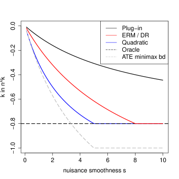
Figure 1: Illustration of the convergence rates in MSE for the estimator considered in this article, as a function of the smoothness $s=\gamma_{1}=\gamma_{2}$. We take the smoothness of the dose-response to be $\alpha=2$ and $\dim(X)=20$.

For smooth functionals possessing a first-order influence function, efficient estimators based on the influence function are asymptotically equivalent. For instance, corrected plug-in estimators and TMLE may be different in finite samples but are asymptotically equivalent. In contrast, for functionals like the dose-response $\theta(t)$, which do not possess influence functions of any order, it is not clear whether estimators based on different approximations of the influence functions are equivalent asymptotically. This is true for higher order corrections as well, particularly for the choice of the projection kernel $\Pi$. For example, $\Pi$ could be taken to represent a projection in $L_{2}(\int K_{ht}(a)p(a,x)da)$, as we have done in this work, or in $L_{2}(p(t,x))$. Using projections in $L_{2}(p(t,x))$ would avoid the assumption that $\int K_{ht}(a)p(a,x)da$ is positive and bounded away from zero, but at the expense of complicating the proof of the theorem, since the arguments made in the proof of Theorem 8.1 in Robins et al. [2017] would need to adjusted to deal with issues such as $\int\Pi(x_{i-1},x_{i})K_{ht}(a_{i})\Pi(x_{i},x_{i+1})d\mathbb{P}(z_{i})\neq\Pi(x_{i-1},x_{i+1})$. Similarly, one may consider replacing $K_{ht}(a)$ with the weight function of a local polynomial regression. That is, replacing $K_{ht}(a)$ with $s(t)^{T}Q^{-1}\widetilde{K}_{ht}(a)s(a)$, where $s(a)=\begin{bmatrix}1&(a-t)&\cdots&(a-t)^{l}\end{bmatrix}^{T}$, $Q=\int\widetilde{K}_{ht}(a)s(a)s(a)^{T}p(a)da$ and $\widetilde{K}(u)$ is a standard second-order kernel, such as the Epanechnikov. An approach conceptually similar to the DR-Learner may use projections in $L_{2}(p(x\mid t))$, although this may require a different analysis than what used to prove Theorem 1. Exploring the differences between these approaches is an important avenue for future work.

4 Sensitivity analysis to the no-unmeasured-confounding assumption

In this section, we briefly outline a simple pseudo-outcome regression method to carry out flexible, nonparametric sensitivity analysis to the no-unmeasured-confounding assumption, i.e., when $Y^{a}\not\perp\!\!\!\perp A\mid X$ so that $\int\mu(t,x)d\mathbb{P}(x)$ can no longer be interpreted as the dose-response curve. To the best of our knowledge, this is the first nonparametric sensitivity analysis method for continuous treatment effects. Bonvini et al. [2022] propose an extension to Rosenbaum’s sensitivity model for binary treatments as follows. Let $U$ be such that $Y^{a}\perp\!\!\!\perp A\mid(X,U)$ and recall that $\mathbb{E}(Y^{a})=\mathbb{E}\{Yp(a)/\pi(a\mid X,U)\mid A=a\}$. Let $\gamma\geq 1$ be a user-specified sensitivity parameter. Departures from the no-unmeasured-confounding assumption are parametrized by considering all densities of $A$ given $(X,U)$, $\pi(a\mid x,u)$, in the class

$$\Pi(\gamma)=\left\{\pi(a\mid x,u):\frac{1}{\gamma}\leq\frac{\pi(a\mid x,u)}{\pi(a\mid x)}\leq\gamma\right\}$$

When $\gamma=1$, corresponding to the case when the measured covariates are sufficient to characterize the treatment selection process, one has the usual identification formula

$$\mathbb{E}(Y^{a})=\mathbb{E}\{w(a,X)Y\mid A=a\}=\int\mu(a,x)d\mathbb{P}(x).$$

Lemma 2 in Bonvini et al. [2022] shows that valid bounds on $\mathbb{E}(Y^{a})$ under the sensitivity model $\Pi(\gamma)$ are

$$\theta_{l}(t;\gamma)=\int\mathbb{E}[Y\gamma^{\operatorname{sgn}\{q_{l}(t,x)-Y\}}\mid A=t,X=x]d\mathbb{P}(x)$$

$$\theta_{u}(t;\gamma)=\int\mathbb{E}[Y\gamma^{\operatorname{sgn}\{Y-q_{u}(t,x)\}}\mid A=t,X=x]d\mathbb{P}(x)$$

where $q_{l}(A,X)$ (resp. $q_{u}(A,X)$) is the $1/(1+\gamma)$ (resp. $\gamma/(1+\gamma)$)-quantile of $Y$ given $(A,X)$. In other words, for a given, user-specified $\gamma$, if $\pi(a\mid x,u)\in\Pi(\gamma)$, then $\theta_{l}(a;\gamma)\leq\mathbb{E}(Y^{a})\leq\theta_{u}(a;\gamma)$.

A DR-Learner estimator of the bounds above can be computed by appropriately modifying the original pseudo-outcome $\varphi(Z)=w(A,X)\{Y-\mu(A,X)\}+\int\mu(A,x)d\mathbb{P}(x)$ and regressing it onto $A$. For $j=\{l,u\}$, define

$$\varphi_{j}(Z;\gamma)\equiv\varphi_{j}(Z;w,\kappa_{j},q_{j},\gamma)=w(A,X)\{s_{j}(Z;q_{j})-\kappa_{j}(A,X;q_{j})\}+\int\kappa_{j}(A,x;q_{j})d\mathbb{P}(x),\text{ for }$$

$$s_{l}(Z;q_{l})=q_{l}(A,X)+\{Y-q_{l}(A,X)\}\gamma^{\operatorname{sgn}\{q_{l}(A,X)-Y\}}$$

$$s_{u}(Z;q_{u})=q_{u}(A,X)+\{Y-q_{u}(A,X)\}\gamma^{\operatorname{sgn}\{Y-q_{u}(A,X)\}}$$

$$\kappa_{j}(A,X;q_{j})=\mathbb{E}\{s_{j}(Z;q_{j})\mid A,X\}$$

Following the sample splitting scheme whereby all nuisance functions are estimated on a separate, independent sample $D^{n}$, a DR-Learner estimator of $\theta_{j}(t;\gamma)$ regresses an estimate of $\varphi_{j}(Z;\gamma)$ onto $A$ on the test set. For example, if the second stage regression is done via linear smoothing, then $\widehat{\theta}_{j}(t;\gamma)=n^{-1}\sum_{i=1}^{n}W_{i}(t;A_{i})\widehat{\varphi}_{j}(Z;\gamma)$. It can be shown that $\varphi_{j}(Z)$ is just part of the influence function of $\int\theta_{j}(a;\gamma)d\mathbb{P}(a)$, which is a pathwise-differentiable parameter. Furthermore, $\varphi_{l}(Z;1)=\varphi_{u}(Z;1)=\varphi(Z)$.

The error analysis of the DR-Learners $\widehat{\theta}_{l}(t;\gamma)$ and $\widehat{\theta}_{u}(t;\gamma)$ follows from Propositions 1 and 2. In this light, it only remains to calculate $\mathbb{E}\{\widehat{\varphi}_{j}(Z;\gamma)-\varphi_{j}(Z;\gamma)\mid A=t,D^{n}\}$. We do so in the following lemma, proved in Appendix D.1, which plays the role of Lemma 1 in the no-unmeasured-confounding case.

Lemma 2.

Let $\widehat{r}_{j}(t)=\mathbb{E}\{\widehat{\varphi}_{j}(Z;\gamma)-\varphi_{j}(Z;\gamma)\mid A=t,D^{n}\}$. It holds that

$$|\widehat{r}_{j}(t)|\ \lesssim\|w-\widehat{w}\|_{t}\|\kappa_{j}-\widehat{\kappa}_{j}\|_{t}+\|q_{j}-\widehat{q}_{j}\|^{2}_{t}+\left|(\mathbb{P}_{n}-\mathbb{P})\widehat{\kappa}_{j}(t,X;\widehat{q}_{j})\right|$$

The result of Lemma 2 is similar to that of Lemma 1, except that the upper bound on the conditional bias involve the additional term $\|q_{j}-\widehat{q}_{j}\|_{t}^{2}$. Thus, consistent estimation of the bounds relies on the consistency of the conditional quantiles estimators. The centered empirical average term is of order $O_{\mathbb{P}}(n^{-1/2})$, under mild boundedness conditions, and thus negligible in nonparametric models for which the convergence rate is slower than $n^{-1/2}$.

We conclude this section by establishing that $\varphi_{j}(Z;\gamma)$ satisfies the doubly-valid structure discovered by Dorn et al. [2021] in a similar sensitivity model for binary treatments. In particular, the bounds remain valid even if the conditional quantiles are not correctly specified. While Dorn et al. [2021] focused on binary treatments, their observation extends to the continuous treatment case as well, as summarized in the following proposition.

Proposition 3.

Let $\overline{w}$, $\overline{\kappa}_{l}$, $\overline{\kappa}_{u}$, $\overline{q}_{l}$ and $\overline{q}_{u}$ be some fixed-functions such that all the expectations below are well defined. If either $\overline{\kappa}_{j}=\kappa_{j}(a,x;\overline{q}_{j})$ or $\overline{w}(a,x)=w(a,x)$, but not necessarily both, then

$$\mathbb{E}\{\varphi_{l}(Z;\overline{w},\overline{\kappa}_{l},\overline{q}_{l},\gamma)\mid A=t\}\leq\theta_{l}(t;\gamma)\leq\theta_{u}(t;\gamma)\leq\mathbb{E}\{\varphi_{u}(Z;\overline{w},\overline{\kappa}_{u},\overline{q}_{u},\gamma)\mid A=t\}$$

Proof.

If either $\overline{\kappa}_{j}=\kappa_{j}(a,x;\overline{q}_{j})$ or $\overline{w}(a,x)=w(a,x)$, then

$$\mathbb{E}\{\varphi_{l}(Z;\overline{w},\overline{\kappa}_{l},\overline{q}_{l},\gamma)\mid A=t\}=\int\left(\overline{q}_{l}(t,x)+\mathbb{E}[\{Y-\overline{q}_{l}(A,X)\}\gamma^{\operatorname{sgn}\{\overline{q}_{l}(A,X)-Y\}}\mid A=t,X=x]\right)d\mathbb{P}(x)$$

$$\mathbb{E}\{\varphi_{u}(Z;\overline{w},\overline{\kappa}_{u},\overline{q}_{u},\gamma)\mid A=t\}=\int\left(\overline{q}_{u}(t,x)+\mathbb{E}[\{Y-\overline{q}_{u}(A,X)\}\gamma^{\operatorname{sgn}\{Y-\overline{q}_{u}(A,X)\}}\mid A=t,X=x]\right)d\mathbb{P}(x)$$

The result follows because it holds that

$$\mathbb{E}\left[\gamma^{\operatorname{sgn}\{q_{l}(A,X)-Y\}}\mid A,X\right]=\mathbb{E}\left[\gamma^{\operatorname{sgn}\{Y-q_{u}(A,X)\}}\mid A,X\right]=1$$

and, deterministically, that

$$\{Y-\overline{q}_{l}(A,X)\}\gamma^{\operatorname{sgn}\{\overline{q}_{l}(A,X)-Y\}}\leq\{Y-\overline{q}_{l}(A,X)\}\gamma^{\operatorname{sgn}\{q_{l}(A,X)-Y\}}$$

$$\{Y-\overline{q}_{u}(A,X)\}\gamma^{\operatorname{sgn}\{Y-\overline{q}_{u}(A,X)\}}\geq\{Y-\overline{q}_{u}(A,X)\}\gamma^{\operatorname{sgn}\{Y-q_{u}(A,X)\}}$$

∎

Proposition 3 establishes the doubly-valid structure of $\varphi_{l}(Z;\gamma)$ and $\varphi_{u}(Z;\gamma)$. Just like in the sensitivity model studied by Dorn et al. [2021] for binary treatments, the bounds on $\mathbb{E}(Y^{a})$ remain valid even if the conditional quantiles are not correctly specified as long as either $w(a,x)$ or the second stage regression of $s_{j}(Z;\overline{q})$ onto $(A,X)$ are.

In the next proposition, we provide the sample analog of Proposition 3 when the estimator of the bounds is a DR-Learner. Let $\overline{\kappa}_{j}(a,x)\equiv\kappa_{j}(a,x;\overline{q}_{j})=\mathbb{E}\{s_{j}(Z;\overline{q}_{j})\mid A=a,X=x\}$. Further, let $R^{2}_{j}(t)$ be the mean-square-error of an oracle estimator of $\theta_{j}(t;\gamma)$ regressing the pseudo-outcome $\overline{\varphi}_{j}(Z;w,\overline{\kappa}_{j},\overline{q}_{j},w,q_{j})$ onto $A$, defined as

$$\overline{\varphi}_{u}(Z;w,\overline{\kappa}_{u},\overline{q}_{u},w,q_{u})=w(A,X)\{s_{u}(Z;\overline{q}_{u})-\overline{\kappa}_{u}(A,X;\overline{q}_{u})\}+\int\overline{\kappa}_{u}(A,x;\overline{q}_{u})d\mathbb{P}(x)$$

$$\hphantom{\overline{\varphi}_{u}(Z;w,\overline{\kappa}_{u},\overline{q}_{u},w,q_{u})=}-w(A,X)\{Y-\overline{q}_{u}(A,X)\}\left[\gamma^{\operatorname{sgn}\{Y-\overline{q}_{u}(A,X)\}}-\gamma^{\operatorname{sgn}\{Y-q_{u}(A,X)\}}\right]$$

$$\overline{\varphi}_{l}(Z;w,\overline{\kappa}_{l},\overline{q}_{l},w,q_{l})=w(A,X)\{s_{l}(Z;\overline{q}_{l})-\overline{\kappa}_{l}(A,X;\overline{q}_{l})\}+\int\overline{\kappa}_{l}(A,x;\overline{q}_{l})d\mathbb{P}(x)$$

$$\hphantom{\overline{\varphi}_{u}(Z;w,\overline{\kappa}_{u},\overline{q}_{u},w,q_{u})=}-w(A,X)\{Y-\overline{q}_{l}(A,X)\}\left[\gamma^{\operatorname{sgn}\{\overline{q}_{l}(A,X)-Y\}}-\gamma^{\operatorname{sgn}\{q_{l}(A,X)-Y\}}\right]$$

It can be shown that $\mathbb{E}\{\overline{\varphi}_{j}(Z;w,\overline{\kappa}_{j},\overline{q}_{j},w,q_{j})\mid A=t\}=\theta_{j}(t;\gamma)$ for $j=\{l,u\}$.

Proposition 4.

Let $\widehat{\theta}_{j}(t;\gamma)$ be an DR-Learner estimator of $\theta_{j}(t;\gamma)$ based on linear smoothing (Sections 2 and 4). Further, let the sample splitting scheme be the same as in Figure 1 and assume that the following conditions hold:

1. If $T_{i}\leq V_{i}$ for all $i\in\{1,\ldots,n\}$, then the weights satisfy $\sum_{i=1}^{n}W_{i}(t;A^{n})T_{i}\leq\sum_{i=1}^{n}W_{i}(t;A^{n})V_{i}$;

2. $\|\widehat{w}-w\|_{\infty}$, $\|\widehat{\kappa}_{j}-\overline{\kappa}_{j}\|_{\infty}$ and $\|\widehat{q}_{j}-\overline{q}_{j}\|_{\infty}$ are all $o_{\mathbb{P}}(1)$, where $\overline{q}_{j}(a,x)$ does not need to equal $q_{j}(a,x)$;

3. $\text{var}\{\overline{\varphi}_{j}(Z;w,\overline{\kappa}_{j},\overline{q}_{u},w,q_{u})\mid A=a\}\geq c>0$ for all $a\in\mathcal{A}$ and some constant $c$.

4. The outcome $Y$ has a uniformly bounded conditional density given any values of $(A,X)$;

5. The linear smoother weights $W_{i}(t;A^{n})$ are localized as in Proposition 2 in a neighborhood $N_{t}$ around $A=t$.

Then, the following inequalities hold

$$\widehat{\theta}_{l}(t;\gamma)\leq\theta_{l}(t;\gamma)+O_{\mathbb{P}}\left(R_{l}(t)+\sup_{a\in N_{t}}r_{l}(a)\right)$$

$$\widehat{\theta}_{u}(t;\gamma)\geq\theta_{u}(t;\gamma)+O_{\mathbb{P}}\left(R_{u}(t)+\sup_{a\in N_{t}}r_{u}(a)\right)$$

where, for $\|f\|^{2}_{t}=\int f^{2}(z)d\mathbb{P}(z\mid A=t)$:

$$r_{j}(t)=\|\widehat{w}-w\|_{t}\|\widehat{\kappa}_{j}-\overline{\kappa}_{j}\|_{t}\ +\ \|\widehat{w}-w\|_{t}\|\widehat{q}_{j}-\overline{q}_{j}\|_{t}\ +\ \left|(\mathbb{P}_{n}-\mathbb{P})\widehat{\kappa}_{j}(t,X;\widehat{q}_{j})\right|$$

Proposition 4 shows that, even if the conditional quantiles of $Y$ given $(A,X)$ are not well estimated, the estimators of the bounds can still converge to functions that contain the region $[\theta_{l}(t;\gamma),\theta_{u}(t;\gamma)]$ and, in this sense, are “valid bounds.” The result holds under mild conditions. For instance, conditions 1 and 5 are a mild stability conditions on the second-stage linear smoother. Conditions 3 and 4 are mild regularity conditions on the data generating process and the nuisance functions’ estimators. The speed at which $\widehat{\theta}_{j}(t;\gamma)$ converges to valid bounds depends on the structural properties of $\theta_{j}(t;\gamma)$, encoded in the oracle MSE $R^{2}_{j}(t)$, as well as the accuracy in estimating $w$ and $\overline{\kappa}$. The proof of Proposition 4 extends the strategy of Dorn et al. [2021] to the case of non-root-$n$ estimable parameters.

5 Small simulation experiment

We conduct a small simulation experiment to evaluate the performance of the first- and second-order estimators in finite samples. We generate data according to the following process

$$X\sim U(-1,1),\quad A\sim\text{TruncNorm}(a_{\min}=-1,a_{\max}=1,\text{ mean}=\kappa(x),\text{ sd}=1),\quad Y\mid A,X\sim N(\xi(a,x),0.25).$$

where $b(x)=\begin{bmatrix}b_{1}(x)&\ldots&b_{6}(x)\end{bmatrix}^{T}$ are the first six, normalized Legendre polynomials and

$$\beta=\begin{bmatrix}1,&0.8,&0.4,&0.2,&0.1,&0.05\end{bmatrix}^{T}$$

$$\kappa(x)=\frac{1}{3}b(x)^{T}\beta\quad\text{ and }\quad\xi(a,x)=b(a)^{T}\beta+b(x)^{T}\beta$$

To estimate $\mu(a,x)$ and $\pi(a\mid x)$ while keeping tight control on the error incurred by the nuisance estimation step, we simulate estimators as

$$\widehat{\mu}(a,x)=\xi(a,x)+N(5n^{-1/\alpha},n^{-1/\alpha})\cdot\cos(2\pi x)+N(5n^{-1/\alpha},n^{-1/\alpha})\cdot\cos(2\pi a)$$

$$\widehat{\pi}(a\mid x)=\phi(a;\text{ mean}=\kappa(x)+N(n^{-1/\alpha},0.5n^{-1/\alpha})\cdot\cos(2\pi x),\text{ sd}=1)$$

for $n=500$ (the sample size used), $\alpha=\{2,4,6,8,10,15\}$ and where $\phi(a;\mu,\sigma^{2})$ is the density of a truncated normal and the terms $N(\mu,\sigma)$ denote independent Normal random variables. The estimators are fluctuations of the true curves where the fluctuations scale as $n^{-1/\alpha}$. We estimate $p(a)$ as $n^{-1}\sum_{i=1}^{n}\widehat{\pi}(a\mid X_{i})$.

As an example of the ERM-based estimator, we consider orthogonal series regression, where the basis that we use is the Legendre polynomials basis. The number of terms ranges from 2 to 8. For the DR-Learner, we consider local linear regression with Gaussian kernel and bandwidth taking value in $\text{bw}=\{0.1,0.2,0.3,0.4,0.5\}$. Finally, we consider first-order (the estimator of Colangelo and Lee [2020]) and second-order estimators based on the higher-order estimator construction. We use a Gaussian kernel for the term $K_{ht}(a)$, with bandwidth taking value in bw and the first eleven Legendre polynomials (normalized) as the basis in $\Pi(x_{i},x_{j})$. We estimate $\Omega$ by its empirical counterpart $\widehat{\Omega}=\mathbb{P}_{n}\{b(X)b(X)^{T}K_{ht}(A)\}$.

To compare the estimators’ performance, we evaluate the dose-response $\theta(a)=b(a)^{T}\beta+\frac{1}{2}\int_{-1}^{1}b(x)^{T}\beta dx$ at 5 points equally spaced in $[-0.5,0.5]$. At each point $t$, we approximate the mean-square-errors of the estimators by averaging their errors across $500$ simulations. At each point $t$, we thus have one estimate of the MSEs for each tuning parameter value (number of basis or bandwidth value). To compare the estimators at each point, we consider the best-performing tuning parameter in terms of MSEs. In practice, this is not viable; potential alternatives would be to select the bandwidth via some form of cross-validation or simply to report a sequence of estimates for tuning parameter value. We finally compute a weighted mean of the MSEs with weight proportional to the density of $A$ at $t$.

Figure 3 reports the results. We have included the MSEs for an oracle DR-Learner estimator that has access to the true nuisance functions to give a reference value. As expected, the performance of the estimators is similar when the error in the nuisance estimators is small. As the error increases, however, the second-order estimator performs better. Across the regimes for the nuisance errors that we considered, the first-order estimator performs better than either the one based on orthogonal series regression (ERM-based) or the one based on local polynomial regression (DR-Learner). In future work, it would be interesting to explore if this conclusion holds even when $\pi(a\mid x)$ and $\mu(a,x)$ have vastly different smoothness levels.

We conclude with a word of caution. In all the results contained in this work, we have not kept track of constant terms. While in asymptotic regimes, constants do not matter, in finite samples they might. Our simulated estimators would thus converge to the truth with the desired rate of order $n^{-1/\alpha}$ even if we consider fluctuations $cn^{-1/\alpha}$ for any constant $c$. Perhaps not surprisingly, we find that our simulation setup is sensitive to the choice of the constants multiplying the rate. In this sense, while encouraging, our limited simulation results should be interpreted with caution. We leave the design and implementation of larger simulation experiments to future work. We refer the reader to Li et al. [2005] for a comprehensive simulation study illustrating the superior performance of estimators based on higher order influence functions in the context of pathwise differentiable parameters.

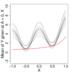
(a) True outcome model $x\mapsto\mathbb{E}(Y\mid A=0,X=x)$ (red) and simulated estimator (black, dotted lines) when $\alpha=8$.

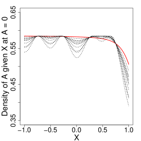
(b) True conditional density $x\mapsto\pi(0\mid X=x)$ (red) and simulated estimators (black, dotted lines) when $\alpha=8$.

Figure 2: Examples of estimators of the true nuisance functions $\mu(a,x)$ and $\pi(a\mid x)$ and simulation results.

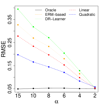
Figure 3: Estimated MSEs for different estimators of the dose-response across 500 simulations.

6 Conclusions and future directions

In this work, we have explored the possibility of improving existing approaches to doubly-robust estimation of a dose-response curve by considering estimators based on DR-Learning framework and higher-order influence functions. We have shown that an estimator akin to the higher-order estimator of the average treatment effect described in Robins et al. [2017] perform better than existing estimators, at least under certain smoothness conditions. In addition, we have specialized recent advancements on regression estimation with estimated outcomes to the dose-response settings and introduced two new doubly-robust estimators of the dose-response curve. A small simulation experiment has corroborated our theoretical results in finite samples. We have also described a flexible method to bound the causal dose-response function in the presence of unmeasured confounding.

Many open questions remain. First, and perhaps most importantly, a minimax lower bound for estimating the dose-response curve has not been described in the literature, to the best of our knowledge. Computing a lower bound on the risk of any estimator of this parameter is instrumental for understanding under what conditions, if any, the higher order estimator that we have proposed can be improved. Second, the higher-order estimator is currently not capable of tracking the smoothness of the dose-response when the conditional density of the treatment given the covariates, viewed as a function of the treatment alone, is less smooth than the dose-response itself. It is unclear if this stems from an intrinsic limitation of our estimator, the upper bound on the risk that we have computed is not tight enough or this is part of the minimax rate. A potential avenue for future research is to investigate the possibility of constructing a higher-order estimator that is based on regressions of some particular pseudo-outcomes onto $A$.

Finally, our results are about convergence of the estimators in mean-square-error. We leave the study of the inferential properties of the estimators discussed here for future work.

Appendix A Proof of Proposition 1

Suppose we observe two samples of $n$ iid observations from $\mathbb{P}$, say $D^{n}$ and $Z^{n}$. Denote $Z_{1},\ldots,Z_{n}$ the observations in $Z^{n}$ that are iid copies of a generic random variable $Z$. Let $U$ denote a generic random variable such that $U\subset Z$. For example, in the dose-response settings, $Z=(Y,A,X)$ and $U=A$. Let $\theta_{0}(u)=\mathbb{E}\{f(Z)\mid U=u\}$ denote the true regression function that needs to be estimated. Recall that $\lVert f\rVert^{2}=\int f(z)^{2}d\mathbb{P}(z)=\mathbb{P}\{f(Z)^{2}\}$ and $\theta^{*}\in\operatorname*{arg\,min}_{\theta\in\Theta}\lVert\theta-\theta_{0}\rVert^{2}$, a fixed function. Let $\widehat{f}(\cdot)$ denote an estimate of $f(\cdot)$ constructed using only observations in $D^{n}$. Let $\mathbb{P}_{n}$ denote the empirical average over sample $Z^{n}$. The estimator of $\theta_{0}(\cdot)$ considered is

$$\widehat{\theta}=\operatorname*{arg\,min}_{\theta\in\Theta}\frac{1}{n}\sum_{i=1}^{n}\{\widehat{f}(Z_{i})-\theta(U_{i})\}^{2}\equiv\operatorname*{arg\,min}_{\theta\in\Theta}\mathbb{P}_{n}\{\widehat{f}(Z)-\theta(U)\}^{2}.$$

Finally, let $\widehat{r}(u)=\mathbb{E}\{\widehat{f}(Z)\mid U=u,D^{n}\}-\theta_{0}(u)$.

The statement of the theorem follows after proving

$$\mathbb{E}(\lVert\widehat{\theta}-\theta_{0}\rVert^{2}\mid D^{n})\lesssim\lVert\widehat{r}\rVert^{2}+\lVert\theta^{*}-\theta_{0}\rVert^{2}+\delta_{n}^{2}$$ (4)

Our proof is a specialization of that of Theorem 3 in Foster and Syrgkanis [2019]. A useful reference for the arguments made in their proof is Chapter 14 in Wainwright [2019]. To prove (4), we need two lemmas.

Lemma 3.

The following inequality holds:

$$\lVert\widehat{\theta}-\theta_{0}\rVert^{2} \leq 8\lVert\widehat{r}\rVert^{2}+3\lVert\theta^{*}-\theta_{0}\rVert^{2}-2(\mathbb{P}_{n}-\mathbb{P})\left[\{\widehat{f}(Z)-\widehat{\theta}(U)\}^{2}-\{\widehat{f}(Z)-\theta^{*}(U)\}^{2}\right]$$

Proof.

Notice that

$$\mathbb{P}\left[\{\widehat{f}(Z)-\widehat{\theta}(U)\}^{2}-\{\widehat{f}(Z)-\theta^{*}(U)\}^{2}\right] =-2\mathbb{P}[\widehat{r}(U)\{\widehat{\theta}(U)-\theta^{*}(U)\}]+\lVert\widehat{\theta}-\theta_{0}\rVert^{2}-\lVert\theta^{*}-\theta_{0}\rVert^{2}$$

By the AM-GM inequality we have, for any $\kappa>0$:

$$2\widehat{r}(U)\{\widehat{\theta}(U)-\theta^{*}(U)\} =2\widehat{r}(U)\{\widehat{\theta}(U)-\theta_{0}(U)\}+2\widehat{r}(U)\{\theta_{0}(U)-\theta^{*}(U)\}$$

$$\leq\frac{2}{\kappa}\widehat{r}(U)^{2}+\kappa\{\widehat{\theta}(U)-\theta_{0}(U)\}^{2}+\kappa\{\theta^{*}(U)-\theta_{0}(U)\}^{2}$$

By monotonicity of integration, it follows that

$$-2\mathbb{P}[\widehat{r}(U)\{\widehat{\theta}(U)-\theta^{*}(U)\}] \geq-\frac{2\|\widehat{r}\|^{2}}{\kappa}-\kappa\lVert\widehat{\theta}-\theta_{0}\rVert^{2}-\kappa\lVert\theta^{*}-\theta_{0}\rVert^{2}$$

Rearranging and choosing $\kappa=1/2$, we have

$$\lVert\widehat{\theta}-\theta_{0}\rVert^{2}\leq 8\lVert\widehat{r}\rVert^{2}+3\lVert\theta^{*}-\theta_{0}\rVert^{2}+2\mathbb{P}\left[\{\widehat{f}(Z)-\widehat{\theta}(U)\}^{2}-\{\widehat{f}(Z)-\theta^{*}(U)\}^{2}\right]$$

Because $\mathbb{P}_{n}[\{\widehat{f}(Z)-\widehat{\theta}(U)\}^{2}-\{\widehat{f}(Z)-\theta^{*}(U)\}^{2}]\leq 0$ since $\theta^{*}\in\Theta$ and $\widehat{\theta}$ is a minimizer, we also have

$$\lVert\widehat{\theta}-\theta_{0}\rVert^{2}\leq 8\lVert\widehat{r}\rVert^{2}+3\lVert\theta^{*}-\theta_{0}\rVert^{2}-2(\mathbb{P}_{n}-\mathbb{P})\left[\{\widehat{f}(Z)-\widehat{\theta}(U)\}^{2}-\{\widehat{f}(Z)-\theta^{*}(U)\}^{2}\right]$$

as desired. ∎

Lemma 4.

For some constant $L$, let

$$\mathcal{E}=\left\{\exists\theta\in\Theta:\lVert\theta-\theta^{*}\rVert\geq\delta_{n}\cap\left|(\mathbb{P}_{n}-\mathbb{P})\left[\{\widehat{f}(Z)-\theta(U)\}^{2}-\{\widehat{f}(Z)-\theta^{*}(U)\}^{2}\right]\right|\geq L\delta_{n}\lVert\theta-\theta^{*}\rVert\right\}$$

Under the conditions of Proposition 1, $\mathbb{P}\left(\mathcal{E}\mid D^{n}\right)\leq c_{1}\exp(-c_{2}n\delta_{n}^{2})$ for some constants $c_{1}$ and $c_{2}$.

Proof.

Consider the sets

$$\mathcal{S}_{m}=\left\{\theta\in\Theta:2^{m-1}\delta_{n}\leq\lVert\theta-\theta^{*}\rVert\leq 2^{m}\delta_{n}\right\}$$

Because $\sup_{\theta\in\Theta}\lVert\theta\rVert_{\infty}\leq S$, $\lVert\theta-\theta^{*}\rVert\leq 2S$ for any $\theta\in\Theta$, which implies that any $\theta$ such that $\lVert\theta-\theta^{*}\rVert\geq\delta_{n}$ must belong to some $\mathcal{S}_{m}$ for $m\in\{1,\ldots,M\}$, where $M\leq\log_{2}(2S/\delta_{n})$. By a union bound,

$$\mathbb{P}(\mathcal{E}\mid D^{n}) \leq\sum_{m=1}^{M}\mathbb{P}(\mathcal{E}\cap\mathcal{S}_{m}\mid D^{n})$$

$$\leq\sum_{m=1}^{M}\mathbb{P}\left(\vphantom{\left|(\mathbb{P}_{n}-\mathbb{P})\left[\{\widehat{f}(Z)-\theta(U)\}^{2}\right]\right|}\exists\theta\in\Theta:\lVert\theta-\theta^{*}\rVert\leq 2^{m}\delta_{n}\right.$$

$$\hphantom{\leq\sum_{m=1}^{M}\mathbb{P}\left(\right.}\quad\left.\cap\left|(\mathbb{P}_{n}-\mathbb{P})\left[\{\widehat{f}(Z)-\theta(U)\}^{2}-\{\widehat{f}(Z)-\theta^{*}(U)\}^{2}\right]\right|\geq 2^{m-1}L\delta^{2}_{n}\mid D^{n}\right)$$

$$\leq\sum_{m=1}^{M}\mathbb{P}(Z_{n}(2^{m}\delta_{n})\geq 2^{m-1}L\delta_{n}^{2}\mid D^{n})$$

where we define

$$Z_{n}(r)=\sup_{\theta\in\Theta:\|\theta-\theta^{*}\|\leq r}\left|(\mathbb{P}_{n}-\mathbb{P})\left[\{\widehat{f}(Z)-\theta(U)\}^{2}-\{\widehat{f}(Z)-\theta^{*}(U)\}^{2}\right]\right|$$

Under the conditions of the proposition, we have

$$\sup_{\theta\in\Theta}\sup_{z\in\mathcal{Z}}\left|\{\widehat{f}(z)-\theta(u)\}^{2}-\{\widehat{f}(z)-\theta^{*}(u)\}^{2}\right|\leq 8S^{2}$$

and

$$\left[\{\widehat{f}(z)-\theta(u)\}^{2}-\{\widehat{f}(z)-\theta^{*}(u)\}^{2}\right]^{2} \leq 16S^{2}\{\theta(u)-\theta^{*}(u)\}^{2}$$

Thus, we have

$$\sigma^{2}(r)\equiv\sup_{\theta:\lVert\theta-\theta^{*}\rVert\leq r}\mathbb{P}\left(\left[\{\widehat{f}(Z)-\theta(U)\}^{2}-\{\widehat{f}(Z)-\theta^{*}(U)\}^{2}\right]^{2}\right)\leq 16S^{2}r^{2}$$

By Theorem 3.27 in Wainwright [2019] and subsequent discussion, viewing $\widehat{f}(\cdot)$ as fixed given $D^{n}$, we have

$$\mathbb{P}\left(Z_{n}(r)\geq\mathbb{E}\{Z_{n}(r)\mid D^{n}\}+u\mid D^{n}\right)\leq 2\exp\left(-\frac{nu^{2}}{8e[16S^{2}r^{2}+16S^{2}\mathbb{E}\{Z_{n}(r)\mid D^{n}\}]+32S^{2}u}\right)$$

Next, we bound $\mathbb{E}\{Z_{n}(r)\mid D^{n}\}$. By a symmetrization argument, for $\epsilon$ a vector of iid Rademacher random variables independent of $Z_{n}$ and $D^{n}$, it holds that

$$\mathbb{E}\{Z_{n}(r)\mid D^{n}\}\leq 2\mathbb{E}_{Z,\epsilon}\left(\sup_{\theta\in\Theta:\|\theta-\theta^{*}\|\leq r}\left|\mathbb{P}_{n}\left(\epsilon\left[\{\widehat{f}(Z)-\theta(U)\}^{2}-\{\widehat{f}(Z)-\theta^{*}(U)\}^{2}\right]\right)\right|\left.\vphantom{\sum}\right|D^{n}\right)$$

The Ledoux-Talagrand contraction inequality (see also pages 147 and 474 in Wainwright [2019]) yields that, for non-random $x_{i}\in\mathcal{X}$, a class $\mathcal{F}$ of real-valued functions and a $L$-Lipschitz function $\phi:\mathbb{R}\to\mathbb{R}$, the following holds

$$\mathbb{E}\left(\sup_{f\in\mathcal{F}}\left|\sum_{i=1}^{n}\epsilon_{i}\{\phi(f(x_{i}))-\phi(f^{*}(x_{i}))\}\right|\right)\leq 2L\mathbb{E}\left(\sup_{f\in\mathcal{F}}\left|\sum_{i=1}^{n}\epsilon_{i}\{f(x_{i})-f^{*}(x_{i})\}\right|\right)$$

where $f^{*}:\mathcal{X}\to\mathbb{R}$ is any function.

Under the boundedness conditions of our proposition, we have

$$\left|\{\widehat{f}(z)-\theta_{1}(u)\}^{2}-\{\widehat{f}(z)-\theta_{2}(u)\}^{2}\right|\leq 4S|\theta_{1}(u)-\theta_{2}(u)|$$

for any $z\in\mathcal{Z}$. Thus, the square-loss in this case is $4S$-Lipschitz for any $z\in\mathcal{Z}$. By the contraction inequality above, we have

$$\mathbb{E}_{\epsilon}\left(\sup_{\theta\in\Theta:\|\theta-\theta^{*}\|\leq r}\left|\mathbb{P}_{n}\left(\epsilon\left[\{\widehat{f}(Z)-\theta(u)\}^{2}-\{\widehat{f}(Z)-\theta^{*}(U)\}^{2}\right]\right)\right|\right)\leq 2\mathbb{E}_{\epsilon}\left(\sup_{\theta\in\Theta:\|\theta-\theta^{*}\|\leq r}\left|\mathbb{P}_{n}[\epsilon\{\theta(U)-\theta^{*}(U)\}]\right|\right)$$

Therefore, we have

$$\mathbb{E}_{Z,\epsilon}\left(\sup_{\theta\in\Theta:\|\theta-\theta^{*}\|\leq r}\left|\mathbb{P}_{n}\left(\epsilon\left[\{\widehat{f}(Z)-\theta(U)\}^{2}-\{\widehat{f}(Z)-\theta^{*}(U)\}^{2}\right]\right)\right|\left.\vphantom{\sum}\right|D^{n}\right)$$

$$\quad\leq 8S\mathbb{E}\left(\sup_{\theta\in\Theta:\|\theta-\theta^{*}\|\leq r}\left|\mathbb{P}_{n}[\epsilon\{\theta(U)-\theta^{*}(U)\}]\right|\left.\vphantom{\sum}\right|D^{n}\right)$$

$$\quad\equiv 8S\mathcal{R}_{n}(\Theta^{*},r)$$

Next, we have assumed $\Theta^{*}$ to be star-shaped; by Lemma 13.6 in Wainwright [2019] the function $r\mapsto\mathcal{R}_{n}(\Theta^{*},r)/r$ is non-increasing. Therefore, because $\delta_{n}$ solves $\mathcal{R}_{n}(\Theta^{*},\delta)\leq\delta^{2}$, we also have:

$$\mathcal{R}_{n}(\Theta^{*},r)\leq r\delta_{n}\quad\text{ for all }r\geq\delta_{n}.$$

Therefore, we conclude that $\mathbb{E}\{Z_{n}(r)\mid D^{n}\}\leq 16Sr\delta_{n}$ for all $r\geq\delta_{n}$.

Putting everything together, we have derived that

$$\mathbb{P}\left(Z_{n}(r)\geq 16Sr\delta_{n}+u\mid D^{n}\right)\leq 2\exp\left(-\frac{nu^{2}}{8e(16S^{2}r^{2}+16^{2}S^{3}r^{2})+32S^{2}u}\right)$$

Let $L=34S$; specializing this bound to our setting with $r=2^{m}\delta_{n}$ and $u=S2^{m}\delta_{n}^{2}$, we have

$$\mathbb{P}\left(Z_{n}(2^{m}\delta_{n})\geq L\cdot 2^{m-1}\delta_{n}^{2}\mid D^{n}\right)\leq 2\exp\left(-\frac{n\delta_{n}^{2}}{8e(16+16^{2}S)+32S}\right)$$

since $2^{-m}\leq 1$ for any $m\geq 1$. Finally,

$$\mathbb{P}(\mathcal{E}\mid D^{n}) \leq\sum_{m=1}^{M}\mathbb{P}\left(Z_{n}(2^{m}\delta_{n})\geq L2^{m-1}\delta_{n}^{2}\mid D^{n}\right)$$

$$\leq 2\exp\left(-\frac{n\delta_{n}^{2}}{8e(16+16^{2}S)+32S}+\ln M\right)$$

Recall that $M\leq\log_{2}(2S/\delta_{n})\leq\log_{2}(2S\sqrt{2n})$ because we have assumed $\delta_{n}\geq 1/\sqrt{2n}$. Therefore, if

$$\delta_{n}^{2}\geq\frac{2\ln\{\log_{2}(2S\sqrt{2n})\}\{8e(16+16^{2}S)+32S\}}{n}$$

we can conclude

$$\mathbb{P}(\mathcal{E}\mid D^{n})\leq 2\exp\left(-\frac{n\delta_{n}^{2}}{16e(16+16^{2}S)+64S}\right)$$

as desired. ∎

A.1   Proof of Equation (4)

Notice that Lemma 4 implies that, with probability at least $1-c_{1}\exp(-c_{2}n\delta_{n}^{2})$, either of the following two events occur:

1. Event 1:

   $$\lVert\widehat{\theta}-\theta^{*}\rVert\leq\delta_{n}\implies\lVert\widehat{\theta}-\theta_{0}\rVert\leq\delta_{n}+\lVert\theta^{*}-\theta_{0}\rVert\implies\lVert\widehat{\theta}-\theta_{0}\rVert^{2}\leq 2\delta_{n}^{2}+2\lVert\theta^{*}-\theta_{0}\rVert^{2}$$

2. Event 2:

   $$\left|(\mathbb{P}_{n}-\mathbb{P})\left[\{\widehat{f}(Z)-\widehat{\theta}(U)\}^{2}-\{\widehat{f}(Z)-\theta^{*}(U)\}^{2}\right]\right| \leq L\delta_{n}\lVert\widehat{\theta}-\theta^{*}\rVert$$

   $$\leq\frac{L^{2}\delta_{n}^{2}}{\kappa}+\frac{\kappa\lVert\widehat{\theta}-\theta_{0}\rVert^{2}}{2}+\frac{\kappa\lVert\theta^{*}-\theta_{0}\rVert^{2}}{2}$$

   for any $\kappa>0$.

Because of the result from Lemma 3, Event 2 (with $\kappa=1/2)$ implies

$$\lVert\widehat{\theta}-\theta_{0}\rVert^{2}\leq 16\lVert\widehat{r}\rVert^{2}+7\lVert\theta^{*}-\theta_{0}\rVert^{2}+8L^{2}\delta_{n}^{2}$$

This means that there exists a constant $C$ such that

$$\mathbb{P}\left(\lVert\widehat{\theta}-\theta_{0}\rVert^{2}\leq C\left(\lVert\widehat{r}\rVert^{2}+\lVert\theta^{*}-\theta_{0}\rVert^{2}+\delta_{n}^{2}\right)\mid D^{n}\right)\geq 1-c_{1}\exp(-c_{2}n\delta_{n}^{2})$$

Let $t_{0}=C\left(\lVert\widehat{r}\rVert^{2}+\lVert\theta^{*}-\theta_{0}\rVert^{2}+\delta_{n}^{2}\right)$. This implies that

$$\mathbb{E}\left(\lVert\widehat{\theta}-\theta_{0}\rVert^{2}\mid D^{n}\right) =\int_{0}^{\infty}\mathbb{P}\left(\lVert\widehat{\theta}-\theta_{0}\rVert^{2}>t\mid D^{n}\right)dt$$

$$=\int_{0}^{t_{0}}\mathbb{P}\left(\lVert\widehat{\theta}-\theta_{0}\rVert^{2}>t\mid D^{n}\right)dt+\int_{t_{0}}^{\infty}\mathbb{P}\left(\lVert\widehat{\theta}-\theta_{0}\rVert^{2}>t\mid D^{n}\right)dt$$

$$=\int_{0}^{t_{0}}\mathbb{P}\left(\lVert\widehat{\theta}-\theta_{0}\rVert^{2}>t\mid D^{n}\right)dt+\int_{0}^{\infty}\mathbb{P}\left(\lVert\widehat{\theta}-\theta_{0}\rVert^{2}>t_{0}+t\mid D^{n}\right)dt$$

$$\leq t_{0}+\int_{0}^{\infty}c_{1}\exp(-c_{3}nt)dt$$

$$=t_{0}+\frac{c_{1}}{c_{3}n}$$

as desired. The last inequality holds because $\mathbb{P}\left(\lVert\widehat{\theta}-\theta_{0}\rVert^{2}>t\mid D^{n}\right)\leq 1$ and because, whenever $\delta_{n}$ satisfies $\mathcal{R}_{n}(\delta_{n};\Theta^{*})/\delta_{n}\leq\delta_{n}$, then so does $\delta_{n}^{\prime}=\sqrt{\delta_{n}^{2}+t/C}>\delta_{n}$. This means that we can write

$$t_{0}+t=C\left(\lVert\widehat{r}\rVert^{2}+\lVert\theta^{*}-\theta_{0}\rVert^{2}+{\delta_{n}^{\prime}}^{2}\right)$$

Thus,

$$\mathbb{P}\left(\lVert\widehat{\theta}-\theta_{0}\rVert^{2}>t_{0}+t\mid D^{n}\right)\leq c_{1}\exp\{-c_{2}n(\delta^{2}_{n}+t/C)\}\leq c_{1}\exp(-c_{3}nt)$$

as Lemma 4 holds for any $\delta^{\prime}_{n}$ that solves $\mathcal{R}_{n}(\delta;\Theta^{*})/\delta\leq\delta$.

Appendix B Proof of Proposition 2

The proof of this theorem is based on Proposition 1 and Theorem 1 from Kennedy [2020]. Their Theorem 1 together with consistency of $\widehat{f}(z)$ yields that

$$|\widehat{\theta}(t)-\theta_{0}(t)|\leq|\widetilde{\theta}(t)-\theta_{0}(t)|+\left|\frac{1}{n}\sum_{i=1}^{n}W_{i}(t;U^{n})\mathbb{E}\{\widehat{f}(Z_{i})-f(Z_{i})\mid D^{n},U_{i}\}\right|+o_{\mathbb{P}}\left(\mathbb{E}\left[\left\{\widetilde{\theta}(t)-\theta_{0}(t)\right\}^{2}\right]\right)$$

Under the assumptions of Proposition 2 (localized weights):

$$\left|\frac{1}{n}\sum_{i=1}^{n}W_{i}(t;U^{n})\widehat{r}(U_{i})\right|\leq\frac{1}{n}\sum_{i=1}^{n}\left|W_{i}(t;U^{n})\right||\widehat{r}(U_{i})|\mathbbm{1}\{U_{i}\in N(t)\}\lesssim\sup_{a\in N(t)}|\widehat{r}(u)|$$

as desired.

Appendix C Proof of Theorem 1

The proof of this theorem essentially follows from that of Theorem 8.1 in Robins et al. [2017], with the main difference that our estimator has $K_{ht}(a)$ in place of $\mathbbm{1}(A=t)$ so that our analysis will need to keep track of terms of order $O(h^{\alpha\land\beta})$.

To simplify the notation, we let $v(a,x)=\mu(a,x)-\widehat{\mu}(a,x),h(a,x)=1/\pi(a\mid x)$, $q(a,x)=\widehat{h}(a,x)-h(a,x)$, $v(x)=v(t,x)$, $q(x)=q(t,x)$, and $g(x)=\int K_{ht}(a)p(a,x)da$. Also we define $\lVert f\rVert^{2}_{g}=\int f^{2}(x)g(x)dx$.

Before computing bias and variance of our estimator, we state some useful facts about orthogonal projections. More general versions of these statements can be found in the excellent supplementary material to Robins et al. [2017]. First, recall the definition of the orthogonal projection and its kernel in our context. For $g(x)=\int K_{ht}(a)p(a,x)da$, $\widehat{g}(x)=\int K_{ht}(a)\widehat{p}(a,x)da$ and some function $f$:

$$\Pi(f)(x_{i})=\int\Pi_{i,j}f(x_{j})g(x_{j})dx_{j}=b(x_{i})^{T}\Omega^{-1}\int b(x_{j})f(x_{j})g(x_{j})dx_{j}$$

$$\widehat{\Pi}(f)(x_{i})=\int\widehat{\Pi}_{i,j}f(x_{j})\widehat{g}(x_{j})dx_{j}=b(x_{i})^{T}\widehat{\Omega}^{-1}\int b(x_{j})f(x_{j})\widehat{g}(x_{j})dx_{j}$$

$$\Omega=\int b(u)b(u)^{T}g(u)du\text{ and }\widehat{\Omega}=\int b(u)b(u)^{T}\widehat{g}(u)du.$$

• Fact 1. Orthogonal projections do not increase length: for any function $f$ and projection in $L_{2}(\mu)$,

  $$\lVert\Pi(f)\rVert^{2}=\int\Pi(f)(x)\Pi(f)(x)d\mu=\int\Pi(f)(x)f(x)d\mu\leq\lVert\Pi(f)\rVert\lVert f\rVert\implies\lVert\Pi(f)\rVert\leq\lVert f\rVert$$

  by Cauchy-Schwarz, where $\lVert f\rVert^{2}=\int f^{2}d\mu$ and $\Pi(f)(x)=b(x)^{T}\left\{\int b(u)b(u)^{T}d\mu\right\}^{-1}\int b(u)f(u)d\mu$.

• Fact 2. Let $w$ denote some positive and bounded weight function and $\Pi_{w}$ and $\Pi$ projections in $L_{2}(\mu)$ onto some fixed $k$-dimensional space $L$ spanned by $b_{1}(x),\ldots,b_{k}(x)$, with weights $w$ and $1$ respectively. Then, for any $l\in L$, we have $\Pi_{w}(l)=\Pi(l)$:

  $$l(x)=b(x)^{T}\beta=\Pi_{w}(l)(x) =b(x)^{T}\left\{\int b(u)b(u)^{T}w(u)d\mu\right\}^{-1}\int b(u)b(u)^{T}\beta w(u)d\mu$$

  $$=b(x)^{T}\left\{\int b(u)b(u)^{T}d\mu\right\}^{-1}\int b(u)b(u)^{T}\beta d\mu=\Pi(l)(x)$$

  where $\beta\in\mathbb{R}^{k}$ is some vector of coefficients.

• Fact 3. Useful identities:

  $$\int\Pi(x_{i},x_{j})\Pi(x_{j},x_{k})g(x_{j})dx_{j}=b(x_{i})^{T}\Omega^{-1}\int b(x_{j})b(x_{j})^{T}g(x_{j})dx_{j}\Omega^{-1}b(x_{k})=\Pi(x_{i},x_{k})$$

  $$\int\widehat{\Pi}(x_{i},x_{j})\widehat{\Pi}(x_{j},x_{k})\widehat{g}(x_{j})dx_{j}=b(x_{i})^{T}\widehat{\Omega}^{-1}\int b(x_{j})b(x_{j})^{T}\widehat{g}(x_{j})dx_{j}\widehat{\Omega}^{-1}b(x_{k})=\widehat{\Pi}(x_{i},x_{k})$$

  $$\int\Pi(x_{i},x_{j})\widehat{\Pi}(x_{j},x_{k})g(x_{j})dx_{j}=b(x_{i})^{T}\Omega^{-1}\int b(x_{j})b(x_{j})^{T}g(x_{j})dx_{j}\widehat{\Omega}^{-1}b(x_{k})=\widehat{\Pi}(x_{i},x_{k})$$

C.1   Bias

We will divide the proof of the bias bound in several steps:

1. Prove that, for some functions $r_{1}$ and $r_{2}$ (defined in the proof) and

   $$T=-\int r_{1}(x_{1})\Pi(x_{1},x_{2})r_{2}(x_{2})g(x_{1})g(x_{2})dx_{1}dx_{2}$$

   the following holds

   $$\left|\int\widehat{\varphi}_{1}(z)d\mathbb{P}(z)-\theta(t)+T\right|\lesssim\lVert(I-\Pi)(v)\rVert_{g}\lVert(I-\Pi)(q)\rVert_{g}+h^{\alpha\land\beta}$$

2. Prove that

   $$\sum_{j=2}^{m}\int\widehat{\varphi}_{j}(z_{1},\ldots,z_{j})d\mathbb{P}(z_{1},\ldots,z_{j})-T$$

   $$=(-1)^{m-1}\int r_{1}(x_{1})(\widehat{\Pi}_{1,2}-\Pi_{1,2})\cdots(\widehat{\Pi}_{m-1,m}-\Pi_{m-1,m})r_{2}(x_{m})g(x_{1})\cdots g(x_{m})dx_{1}\cdots dx_{m}$$

   $$\equiv T_{2}$$

3. Prove that

   $$\left|T_{2}\right|\lesssim\lVert r_{1}\rVert_{g}\lVert r_{2}\rVert_{g}\lVert\widehat{s}-1\rVert^{m-1}_{\infty}\lesssim\left(\lVert v\rVert_{g}\lVert q\rVert_{g}+h^{\alpha\land\beta}\right)\lVert\widehat{s}-1\rVert^{m-1}_{\infty}$$

   where $\widehat{s}=g/\widehat{g}$.

C.1.1 Step 1

Let us define

$$\Delta_{1}(x)\equiv\int K_{ht}(a)\{v(a,x)-v(t,x)\}\pi(a\mid x)da$$

$$\Delta_{2}(x)\equiv\int K_{ht}(a)\{\mu(a,x)-\mu(t,x)\}\pi(a\mid x)da$$

$$\Delta_{3}(x)\equiv\int K_{ht}(a)\{\widehat{h}(a,x)-\widehat{h}(t,x)\}\pi(a\mid x)da$$

$$\Delta_{4}(x)\equiv\int K_{ht}(a)\pi(a\mid x)da-\pi(t\mid x)$$

$$\Delta_{5}(x)\equiv h(t,x)-\frac{1}{\int K_{ht}(a)\pi(a\mid x)da}=\frac{\Delta_{4}(x)}{\pi(t\mid x)\{\pi(t\mid x)+\Delta_{4}(x)\}}$$

We have

$$\int\widehat{\varphi}_{1}(z)d\mathbb{P}(z)-\theta(t) =\int K_{ht}(a)\widehat{h}(t,x)\{\mu(a,x)-\widehat{\mu}(t,x)\}\pi(a\mid x)dap(x)dx-\int v(x)p(x)dx$$

$$=\int K_{ht}(a)\widehat{h}(t,x)\{\mu(a,x)-\widehat{\mu}(t,x)\}\pi(a\mid x)dap(x)dx-\int\frac{v(x)}{\int K_{ht}(a)\pi(a\mid x)da}g(x)dx$$

$$=\int v(x)q(x)g(x)dx+\int v(x)\Delta_{5}(x)g(x)dx+\int\widehat{h}(t,x)\Delta_{2}(x)p(x)dx$$

Let

$$r_{1}(x)=v(x)+\frac{\Delta_{1}(x)}{\int K_{ht}(a)\pi(a\mid x)da},\text{ and }r_{2}(x)=q(x)+\Delta_{5}(x)+\frac{\Delta_{3}(x)}{\int K_{ht}(a)\pi(a\mid x)da}$$

and notice that

$$\int K_{ht}(a)\{y-\widehat{\mu}(a,x)\}d\mathbb{P}(z\mid x)=r_{1}(x)\int K_{ht}(a)\pi(a\mid x)da$$

$$\int\{K_{ht}(a)\widehat{h}(a,x)-1\}d\mathbb{P}(z\mid x)=r_{2}(x)\int K_{ht}(a)\pi(a\mid x)da$$

Define

$$T \equiv-\int r_{1}(x_{1})\Pi(x_{1},x_{2})r_{2}(x_{2})g(x_{1})dx_{1}g(x_{2})dx_{2}$$

$$=-\int v(x)\Pi(q)(x)g(x)dx-\int\frac{\Delta_{1}(x)}{\int K_{ht}(a)\pi(a\mid x)da}\Pi(r_{2})(x)g(x)dx$$

$$\hphantom{=}\ -\int\Pi(v)(x)\left\{\Delta_{5}(x)+\frac{\Delta_{3}(x)}{\int K_{ht}(a)\pi(a\mid x)da}\right\}g(x)dx$$

Therefore,

$$\int\widehat{\varphi}_{1}(z)d\mathbb{P}(z)+T-\theta(t)=\int v(x)(I-\Pi)(q)(x)g(x)dx+\Delta$$

where $\Delta$ groups all the terms involving $\Delta_{j}$ together:

$$\Delta =\int v(x)\Delta_{5}(x)g(x)dx+\int\widehat{h}(t,x)\Delta_{2}(x)p(x)dx$$

$$\hphantom{=}\ -\int\frac{\Delta_{1}(x)}{\int K_{ht}(a)\pi(a\mid x)da}\Pi(r_{2})(x)g(x)dx-\int\Pi(v)(x)\left\{\Delta_{5}(x)+\frac{\Delta_{3}(x)}{\int K_{ht}(a)\pi(a\mid x)da}\right\}g(x)dx$$

The term $\Delta$ is controlled under the smoothness assumptions of the theorem, while

$$\left|\int v(x)(I-\Pi)(q)(x)g(x)dx\right|\leq\lVert(I-\Pi)(v)\rVert_{g}\lVert(I-\Pi)(q)\rVert_{g}$$

by Cauchy-Schwarz. In particular, we have assumed that $a\mapsto\mu(a,x)$, $a\mapsto\widehat{\mu}(a,x)$ are $\alpha$-times continuously differentiable and $a\mapsto h(a,x)$, $a\mapsto\widehat{h}(a,x)$ (or, equivalently, $\pi(a\mid x)$ and $\widehat{\pi}(a\mid x)$) are $\beta$-times continuously differentiable. Thus, we have

$$v(a,x)=\sum_{j=0}^{\alpha-1}v^{(j)}(t,x)\frac{(a-t)^{j}}{j!}+v^{(\alpha)}(t+\tau_{1}(a-t),x)\frac{(a-t)^{\alpha}}{\alpha!}$$

$$\mu(a,x)=\sum_{j=0}^{\alpha-1}\mu^{(j)}(t,x)\frac{(a-t)^{j}}{j!}+\mu^{(\alpha)}(t+\tau_{2}(a-t),x)\frac{(a-t)^{\alpha}}{\alpha!}$$

$$\pi(a\mid x)=\sum_{j=0}^{\beta-1}\pi^{(j)}(t\mid x)\frac{(a-t)^{j}}{j!}+\pi^{(\beta)}(t+\tau_{3}(a-t)\mid x)\frac{(a-t)^{\beta}}{\beta!}$$

$$h(a,x)=\sum_{j=0}^{\beta-1}h^{(j)}(t,x)\frac{(a-t)^{j}}{j!}+h^{(\beta)}(t+\tau_{4}(a-t),x)\frac{(a-t)^{\beta}}{\beta!}$$

for some $\tau_{1},\tau_{2},\tau_{3},\tau_{4}\in[0,1]$. Then, for example, we have the following

$$\Delta_{1}(x) \equiv\int K_{ht}(a)\{v(a,x)-v(t,x)\}\pi(a\mid x)da$$

$$=\sum_{i=1}^{\alpha-1}\sum_{j=0}^{\beta-1}h^{i+j}\frac{v^{(i)}(t,x)}{i!}\frac{\pi^{(j)}(t\mid x)}{j!}\int_{0}^{1}u^{i+j}K(u)du$$

$$\hphantom{=}+\sum_{j=1}^{\alpha-1}h^{\beta+j}\frac{v^{(j)}(t,x)}{\beta!j!}\int_{0}^{1}u^{\beta+j}K(u)\pi^{(\beta)}(t+\tau_{3}uh\mid x)du$$

$$\hphantom{=}+\sum_{j=0}^{\beta-1}h^{\alpha+j}\frac{\pi^{(j)}(t\mid x)}{\alpha!j!}\int_{0}^{1}v^{(\alpha)}(t+\tau_{1}uh,x)u^{\alpha+j}K(u)du$$

$$\hphantom{=}+\frac{h^{\alpha+\beta}}{\alpha!\beta!}\int_{0}^{1}v^{(\alpha)}(t+\tau_{1}uh,x)u^{\alpha+\beta}K(u)\pi^{(\beta)}(t+\tau_{3}uh\mid x)du$$

so that $\lVert\Delta_{1}\rVert_{\infty}\lesssim h^{(\beta+1)\land\alpha}$. Similarly, $\lVert\Delta_{2}\rVert_{\infty}\lesssim h^{(\beta+1)\land\alpha}$ and

$$\Delta_{3}(x) \equiv\int K_{ht}(a)\{\widehat{h}(a,x)-\widehat{h}(t,x)\}\pi(a\mid x)da$$

$$=\sum_{i=1}^{\beta-1}\sum_{j=0}^{\beta-1}h^{i+j}\frac{\widehat{h}^{(i)}(t,x)}{i!}\frac{\pi^{(j)}(t\mid x)}{j!}\int_{0}^{1}u^{i+j}K(u)du$$

$$\hphantom{=}+\sum_{j=1}^{\beta-1}h^{\beta+j}\frac{\widehat{h}^{(j)}(t,x)}{\beta!j!}\int_{0}^{1}u^{\beta+j}K(u)\pi^{(\beta)}(t+\tau_{3}uh\mid x)du$$

$$\hphantom{=}+\sum_{j=0}^{\beta-1}h^{\beta+j}\frac{\pi^{(j)}(t\mid x)}{\beta!j!}\int_{0}^{1}\widehat{h}^{(\beta)}(t+\tau_{1}uh,x)u^{\beta+j}K(u)du$$

$$\hphantom{=}+\frac{h^{2\beta}}{\beta!\beta!}\int_{0}^{1}v^{(\beta}(t+\tau_{1}uh,x)u^{2\beta}K(u)\pi^{(\beta)}(t+\tau_{3}uh\mid x)du$$

Therefore, $\lVert\Delta_{3}\rVert_{\infty}\lesssim h^{\beta}$ and, similarly, $\lVert\Delta_{4}\rVert_{\infty}\lesssim h^{\beta}$ and $\lVert\Delta_{5}\rVert_{\infty}\lesssim h^{\beta}$. In this light, it holds that $\lVert\Delta_{j}\rVert_{\infty}\lesssim h^{\alpha\land\beta}$, for $j=1,2,3,4,5$. This concludes our proof that

$$\left|\int\widehat{\varphi}_{1}(z)d\mathbb{P}(z)+T-\theta(t)\right|\lesssim\lVert(I-\Pi)(v)\rVert_{g}\lVert(I-\Pi)(q)\rVert_{g}+h^{\alpha\land\beta}$$

C.1.2 Step 2

We will show that

$$T_{2} =\sum_{j=2}^{m}\int\widehat{\varphi}_{j}(z_{1},\ldots,z_{j})d\mathbb{P}(z_{1},\ldots,z_{j})-T$$

$$=\sum_{j=2}^{m}\int\widehat{\varphi}_{j}(z_{1},\ldots,z_{j})d\mathbb{P}(z_{1},\ldots,z_{j})+\int r_{1}(x)\Pi(x_{1},x_{2})r_{2}(x_{2})g(x_{1})g(x_{2})dx_{1}dx_{2}$$

$$=(-1)^{m-1}\int r_{1}(x_{1})(\widehat{\Pi}_{1,2}-\Pi_{1,2})\cdots(\widehat{\Pi}_{m-1,m}-\Pi_{m-1,m})r_{2}(x_{m})g(x_{1})\cdots g(x_{m})dx_{1}\cdots dx_{m}$$

The result is clearly true for $m=2$, so we proceed by induction. Relative to the $m^{\text{th}}$ term, the term $m+1$ receives the contribution from

$$\int\widehat{\varphi}_{m+1}(z_{1},\ldots,z_{m+1})d\mathbb{P}(z_{1},\ldots,z_{m})$$

$$=(-1)^{m}\sum_{i=0}^{m-1}{{m-1}\choose i}(-1)^{i}\int r_{1}(x_{1})\widehat{\Pi}_{1,2}\cdots\widehat{\Pi}_{m-i,m-i+1}r_{2}(x_{m-i+1})g(x_{1})\cdots g(x_{m-i+1})dx_{1}\cdots dx_{m-i+1}$$

$$\equiv(-1)^{m}T_{3}$$

Thus to prove the claim we need to show that

$$T_{3} =\int r_{1}(x_{1})(\widehat{\Pi}_{1,2}-\Pi_{1,2})\cdots(\widehat{\Pi}_{m-1,m}-\Pi_{m-1,m})r_{2}(x_{m})g(x_{1})\cdots g(x_{m})dx_{1}\cdots dx_{m}$$

$$\hphantom{=}+\int r_{1}(x_{1})(\widehat{\Pi}_{1,2}-\Pi_{1,2})\cdots(\widehat{\Pi}_{m,m+1}-\Pi_{m,m+1})r_{2}(x_{m+1})g(x_{1})\cdots g(x_{m+1})dx_{1}\cdots dx_{m+1}$$

$$\equiv T_{4}+T_{5}$$

Notice that $T_{4}$ can be written as a sum of terms of the form

$$B_{l}=(-1)^{m-1-l}\int r_{1}(x_{1})B_{1,2}\cdots B_{m-1,m}r_{2}(x_{m})g(x_{1})\cdots g(x_{m})dx_{1}\cdots dx_{m}$$

where $B_{i,j}$ equals either $\widehat{\Pi}_{i,j}$ or $\Pi_{i,j}$ and $l$ denotes the number of terms in the product for which $B_{i,j}=\widehat{\Pi}_{i,j}$. Similarly, $T_{5}$ is a sum of terms of the form

$$C_{l}=(-1)^{m-l}\int r_{1}(x_{1})B_{1,2}\cdots B_{m,m+1}r_{2}(x_{m+1})g(x_{1})\cdots g(x_{m+1})dx_{1}\cdots dx_{m+1}$$

Fact 3 is the reason why we only need to keep track of the number of $\widehat{\Pi}_{i,j}$ terms and not specifically which $B_{ij}$ equals $\Pi_{i,j}$ or $\widehat{\Pi}_{i,j}$. In fact, for $B_{ij}=\Pi_{i,j}$ or $\widehat{\Pi}_{i,j}$, we have

$$\int\Pi(x_{j-1},x_{j})B(x_{j},x_{j+1})g(x_{j})dx_{j}=B_{j-1,j+1}=\int B(x_{j-1},x_{j})\Pi(x_{j},x_{j+1})g(x_{j})dx_{j}$$

In this light, we can simplify as

$$B_{l}=(-1)^{m-1-l}\int r_{1}(x_{1})\widehat{\Pi}_{1,2}\cdots\widehat{\Pi}_{l,l+1}r_{2}(x_{l+1})dg(x_{1})\cdots dg(x_{l+1})\text{ for }l\geq 1$$

$$B_{0}=(-1)^{m-1}\int r_{1}(x_{1})\Pi_{1,2}r_{2}(x_{2})dg(x_{1})d(x_{2})$$

$$C_{l}=(-1)^{m-l}\int r_{1}(x_{1})\widehat{\Pi}_{1,2}\cdots\widehat{\Pi}_{l,l+1}r_{2}(x_{l+1})dg(x_{1})\cdots dg(x_{l+1})\text{ for }l\geq 1$$

$$C_{0}=(-1)^{m}\int r_{1}(x_{1})\Pi_{1,2}r_{2}(x_{2})dg(x_{1})d(x_{2})=-B_{0}$$

For $l\in\{1,\ldots,m-1\}$, we have $C_{l}=-B_{l}$. Thus, we have reached

$$T_{4}=-C_{0}-\sum_{l=1}^{m-1}{m-1\choose l}C_{l}\quad\text{ and }\quad T_{5}=C_{0}+\sum_{l=1}^{m-1}{m\choose l}C_{l}+C_{m}$$

and this implies

$$T_{4}+T_{5} =\sum_{l=1}^{m-1}\left\{{m\choose l}-{m-1\choose l}\right\}C_{l}+C_{m}=\sum_{l=1}^{m-1}{m-1\choose l-1}C_{l}+C_{m}=T_{3}$$

as desired. We have thus shown that

$$T_{2}=(-1)^{m-1}\int r_{1}(x_{1})(\widehat{\Pi}_{1,2}-\Pi_{1,2})\cdots(\widehat{\Pi}_{m-1,m}-\Pi_{m-1,m})r_{2}(x_{m})g(x_{1})\cdots g(x_{m})dx_{1}\cdots dx_{m}$$

C.1.3 Step 3

We need to show that $|T_{2}|\ \leq\lVert r_{1}\rVert_{g}\lVert r_{2}\rVert_{g}\lVert\widehat{s}-1\rVert_{\infty}^{m-1}$. This statement is essentially a direct consequence of Lemma 13.7 in the Supplementary material to Robins et al. [2017]. For the sake of completeness, we give a proof here that is less general (and more verbose) than that in Robins et al. [2017], although it uses the same arguments.

Define $\widehat{s}=g(x)/\widehat{g}(x)$ and let $M_{\widehat{s}}$ denoting multiplication by $\widehat{s}$. We have

$$\int(\widehat{\Pi}_{m-1,m}-\Pi_{m-1,m})r_{2}(x_{m})g(x_{m})dx_{m}=\left(\widehat{\Pi}M_{\widehat{s}}-\Pi\right)(r_{2})(x_{m-1})$$

Continuing with this calculation, we get

$$T_{2}=(-1)^{m-1}\int r_{1}(x)\left(\widehat{\Pi}M_{\widehat{s}}-\Pi\right)^{m-1}(r_{2})(x)g(x)dx$$

Let $\lVert f\rVert^{2}_{2,\widehat{g}}=\int f^{2}(u)\widehat{g}(u)du$ and bound $|T_{2}|$ as

$$|T_{2}|\ \lesssim\ \|r_{1}\|_{g}\left\|\left(\widehat{\Pi}M_{\widehat{s}}-\Pi\right)^{m-1}(r_{2})\right\|_{2,\widehat{g}}$$

Define

$$l(x)=\left(\widehat{\Pi}M_{\widehat{s}}-\Pi\right)^{m-2}(r_{2})(x)\equiv b(x)^{T}\beta$$

We can write $l(x)$ as a linear combination of the truncated basis because both $\widehat{\Pi}$ and $\Pi$ project a function onto the same finite dimensional subspace. Notice that we can view $\Pi$ as a weighted projection in $L_{2}(\widehat{g})$ with weight $\widehat{s}$, i.e.

$$\Pi(f)(x)=b(x)^{T}\Omega^{-1}\int b(u)f(u)g(u)du=b(x)^{T}\left\{\int b(u)b(u)\widehat{s}(u)\widehat{g}(u)du\right\}^{-1}\int b(u)f(u)\widehat{s}(u)\widehat{g}(u)du$$

Therefore, by Fact 2, we have

$$\left(\widehat{\Pi}M_{\widehat{s}}-\Pi\right)^{m-1}(r_{2})(x) =\left(\widehat{\Pi}M_{\widehat{s}}-\Pi\right)(l)(x)=\int\widehat{\Pi}(x,u)\{\widehat{s}(u)-1\}l(u)\widehat{g}(u)du=\widehat{\Pi}\left((\widehat{s}-1)l\right)(x)$$

By Fact 1, we have

$$\left\|\left(\widehat{\Pi}M_{\widehat{s}}-\Pi\right)^{m-1}(r_{2})\right\|_{2,\widehat{g}}=\left\|\widehat{\Pi}\left((\widehat{s}-1)l\right)\right\|_{2,\widehat{g}}\leq\lVert(\widehat{s}-1)l\rVert_{2,\widehat{g}}\leq\lVert\widehat{s}-1\rVert_{\infty}\lVert l\rVert_{2,\widehat{g}}$$

Repeating this argument $m-3$ times applied to $\lVert l\rVert_{2,\widehat{g}}$, we obtain

$$\left\|\left(\widehat{\Pi}M_{\widehat{s}}-\Pi\right)^{m-1}(r_{2})\right\|_{2,\widehat{g}}\leq\lVert\widehat{s}-1\rVert^{m-2}_{\infty}\left\|\left(\widehat{\Pi}M_{\widehat{s}}-\Pi\right)(r_{2})\right\|_{2,\widehat{g}}$$

Furthermore,

$$\left\|\left(\widehat{\Pi}M_{\widehat{s}}-\Pi\right)(r_{2})\right\|^{2}_{2,\widehat{g}} =\int\left(\widehat{\Pi}M_{\widehat{s}}-\Pi\right)(r_{2})(x)\left(\widehat{\Pi}M_{\widehat{s}}-\Pi\right)(r_{2})(x)\widehat{g}(x)dx$$

$$=\int\left(\widehat{\Pi}M_{\widehat{s}}-\Pi\right)(r_{2})(x)\Pi\left(r_{2}\right)(x)\{\widehat{s}(x)-1\}\widehat{g}(x)dx$$

The second line follows because $\left(\widehat{\Pi}M_{\widehat{s}}-\Pi\right)(r_{2})$ belongs to the finite dimensional subspace and can be expressed as $b(x)^{T}\beta$ for some $\beta$. Therefore,

$$\int\left(\widehat{\Pi}M_{\widehat{s}}-\Pi\right)(r_{2})(x)\widehat{\Pi}M_{\widehat{s}}(r_{2})(x)\widehat{g}(x)dx =\beta^{T}\int b(x)\widehat{\Pi}M_{\widehat{s}}(r_{2})(x)\widehat{g}(x)dx$$

$$=\beta^{T}\int b(x)b(x)^{T}\widehat{\Omega}^{-1}\int b(u)\widehat{s}(u)r_{2}(u)\widehat{g}(u)du\widehat{g}(x)dx$$

$$=\beta^{T}\int b(u)r_{2}(u)g(u)du$$

$$=\beta^{T}\int b(x)b(x)^{T}\Omega^{-1}\int b(u)r(u)g(u)du\widehat{s}(x)\widehat{g}(x)dx$$

$$=\int\beta^{T}b(x)\Pi(r_{2})(x)\widehat{s}(x)\widehat{g}(x)dx$$

By Cauchy-Schwarz:

$$\left\|\left(\widehat{\Pi}M_{\widehat{s}}-\Pi\right)(r_{2})\right\|^{2}_{2,\widehat{g}}\leq\left\|\left(\widehat{\Pi}M_{\widehat{s}}-\Pi\right)(r_{2})\right\|_{2,\widehat{g}}\left\|\Pi\left(r_{2}\right)(\widehat{s}-1)\right\|_{2,\widehat{g}},$$

implying

$$\left\|\left(\widehat{\Pi}M_{\widehat{s}}-\Pi\right)(r_{2})\right\|_{2,\widehat{g}}\lesssim\lVert\widehat{s}-1\rVert_{\infty}\lVert r_{2}\rVert_{g}.$$

This then yields

$$\left|T_{2}\right|\lesssim\lVert r_{1}\rVert_{g}\lVert r_{2}\rVert_{g}\lVert\widehat{s}-1\rVert^{m-1}_{\infty}.$$

The bounds on the terms involving $\Delta_{j}$ derived in Step 1 finally yield the result:

$$|T_{2}|\ \lesssim\left(\lVert v\rVert_{g}\lVert q\rVert_{g}+h^{\alpha\land\beta}\right)\lVert\widehat{s}-1\rVert_{\infty}^{m-1}$$

C.2   Variance

The proof of the variance bound follows as in Robins et al. [2017]. Because, for two random variables $U_{1}$ and $U_{2}$, $\text{var}(U_{1}+U_{2})\leq 2\text{var}(U_{1})+2\text{var}(U_{2})$, and because $m$ is fixed, we have:

$$\text{var}\left\{\mathbb{P}_{n}\widehat{f}_{0}(Z)+\sum_{j=2}^{m}\mathbb{U}_{n}\widehat{\varphi}_{j}(Z_{1},\ldots,Z_{j})\mid D^{n}\right\} \leq 2\text{var}\left\{\mathbb{P}_{n}\widehat{f}_{0}(Z)\mid D^{n}\right\}+2\text{var}\left\{\sum_{j=2}^{m}\mathbb{U}_{n}\widehat{\varphi}_{j}(Z_{1},\ldots,Z_{j})\mid D^{n}\right\}$$

$$\lesssim\text{var}\left\{\mathbb{P}_{n}\widehat{f}_{0}(Z)\mid D^{n}\right\}+P^{n}\left[\left\{\sum_{j=2}^{m}\mathbb{U}_{n}\widehat{\varphi}_{j}(Z_{1},\ldots,Z_{j})\right\}^{2}\right]$$

$$\lesssim\text{var}\left\{\mathbb{P}_{n}\widehat{f}_{0}(Z)\mid D^{n}\right\}+\sum_{j=2}^{m}P^{n}\left[\left\{\mathbb{U}_{n}\widehat{\varphi}_{j}(Z_{1},\ldots,Z_{j})\right\}^{2}\right]$$

Because, given $D^{n}$, $\mathbb{P}_{n}\widehat{f}_{0}(Z)$ is a sample average of independent observations, we have

$$\text{var}\left\{\mathbb{P}_{n}\widehat{f}_{0}(Z)\mid D^{n}\right\}\leq\frac{1}{n}\mathbb{P}\{\widehat{f}^{2}_{0}(Z)\}\lesssim\frac{1}{nh}$$

since $\int K^{2}_{ht}(a)\pi(a\mid x)da=h^{-1}\int K^{2}(u)\pi(uh+t)du\lesssim h^{-1}$. By Lemma 14.1 in Robins et al. [2017], the following holds

$$P^{n}\left[\left\{\mathbb{U}_{n}\widehat{\varphi}_{j}(Z_{1}\ldots,Z_{j})\right\}^{2}\right]\leq 2j\left(1+\left\|\frac{p}{\widehat{p}}\right\|_{\infty}\right)^{2j}\widehat{P}^{n}\left[\left\{\mathbb{U}_{n}\widehat{\varphi}_{j}(Z_{1}\ldots,Z_{j})\right\}^{2}\right]$$

Because $\widehat{\varphi}_{j}$ is degenerate relative to $\widehat{P}$, we also have

$$\widehat{P}^{n}\left[\left\{\mathbb{U}_{n}(\widehat{\varphi}_{j}(Z_{1}\ldots,Z_{j}))\right\}^{2}\right] \lesssim\frac{1}{n(n-1)\cdots(n-j+1)}\widehat{P}^{j}\left[\left\{\widehat{\varphi}_{j}(Z_{1}\ldots,Z_{j})\right\}^{2}\right]$$

$$\lesssim\frac{1}{n(n-1)\cdots(n-j+1)}\widehat{P}^{j}\left[\left\{f_{1}(Z_{1})\widehat{\Pi}_{1,2}K_{ht}(A_{2})\cdots\widehat{\Pi}_{j-1,j}f_{2}(Z_{j})\right\}^{2}\right]$$

Notice that

$$\left\{f_{1}(Z_{1})\widehat{\Pi}_{1,2}K_{ht}(A_{2})\cdots\widehat{\Pi}_{j-1,j}f_{2}(Z_{j})\right\}^{2}\lesssim K^{2}_{ht}(A_{1})\widehat{\Pi}^{2}_{1,2}K^{2}_{ht}(A_{2})\cdots\widehat{\Pi}^{2}_{j-1,j}K^{2}_{ht}(A_{j})$$

since $h(a,x)$, $Y$ and $\widehat{\mu}(a,x)$ are uniformly bounded by assumption. Next, because

$$\int K^{2}_{ht}(a)\pi(a\mid x)da=h^{-1}\int K^{2}(u)\pi(uh+t\mid x)du\lesssim h^{-1},$$

we have

$$\widehat{P}^{j}\left[\left\{f_{1}(Z_{1})\widehat{\Pi}_{1,2}K_{ht}(A_{2})\cdots\widehat{\Pi}_{j-1,j}f_{2}(Z_{j})\right\}^{2}\right] \lesssim h^{-j}\int\widehat{\Pi}^{2}_{1,2}\cdots\widehat{\Pi}^{2}_{j-1,j}p(x_{1})\cdots p(x_{j})dx_{1}\cdots dx_{j}$$

$$=h^{-j}\int\widehat{\Pi}^{2}_{1,2}\cdots\widehat{\Pi}^{2}_{j-1,j}\left\{\prod_{l=1}^{j}\frac{p(x_{l})}{\widehat{g}(x_{l})}\right\}\widehat{g}(x_{1})\cdots\widehat{g}(x_{j})dx_{1}\cdots dx_{j}$$

$$\leq\left\{\sup_{x}\frac{p(x)}{\widehat{g}(x)}\right\}^{j}h^{-j}\int\widehat{\Pi}^{2}_{1,2}\cdots\widehat{\Pi}^{2}_{j-1,j}\widehat{g}(x_{1})\cdots\widehat{g}(x_{j})dx_{1}\cdots dx_{j}$$

$$\lesssim h^{-j}\int\widehat{\Pi}^{2}_{1,2}\cdots\widehat{\Pi}^{2}_{j-1,j}\widehat{g}(x_{1})\cdots\widehat{g}(x_{j})dx_{1}\cdots dx_{j}$$

Next, notice that

$$\int\widehat{\Pi}^{2}(x_{i},x_{j})\widehat{g}(x_{j})dx_{j}=\int b(x_{i})^{T}\widehat{\Omega}^{-1}b(x_{j})b(x_{j})^{T}\widehat{\Omega}^{-1}b(x_{i})\widehat{g}(x_{j})dx_{j}=\widehat{\Pi}(x_{i},x_{i})$$

We bound each term from $i=j$ to $i=3$ as

$$\int\widehat{\Pi}^{2}_{i-2,i-1}\widehat{\Pi}^{2}_{i-1,i}\widehat{g}(x_{i-1})\widehat{g}(x_{i})dx_{i-1}dx_{i} =\int\widehat{\Pi}^{2}_{i-2,i-1}\widehat{\Pi}_{i-1,i-1}\widehat{g}(x_{i-1})dx_{i-1}$$

$$\leq\sup_{x}\widehat{\Pi}(x,x)\int\widehat{\Pi}^{2}_{i-2,i-1}\widehat{g}(x_{i-1})dx_{i-1}$$

This leads to

$$\int\widehat{\Pi}^{2}_{1,2}\cdots\widehat{\Pi}^{2}_{j-1,j}\widehat{g}(x_{1})\cdots\widehat{g}(x_{j})dx_{1}\cdots dx_{j}\leq\left\{\sup_{x}\widehat{\Pi}(x,x)\right\}^{j-2}\int\widehat{\Pi}^{2}_{1,2}\widehat{g}(x_{1})dx_{1}\widehat{g}(x_{2})dx_{2}$$

Finally, without loss of generality, let $b(x)$ be scaled so that $\widehat{\Omega}$ is the identity matrix. This way, we immediately have

$$\int\widehat{\Pi}^{2}_{1,2}\widehat{g}(x_{1})\widehat{g}(x_{2})dx_{1}dx_{2}=\int b(x)^{T}b(x)\widehat{g}(x)dx=\sum_{i=1}^{k}\int b^{2}_{i}(x)\widehat{g}(x)dx=k$$

because the basis is orthonormal. Because $m$ is fixed and does not grow with $n$ and $\sup_{x}\widehat{\Pi}(x,x)\lesssim k$, this yields the bounds in the statement of the theorem.

Appendix D Proofs of claims from Section 4

D.1   Proof of Lemma 2

We prove the result for the upper bound, as that for the lower bound can be proven with a similar argument. By Leibniz rule of integration, the derivative of the map $\overline{q}(a,x)\mapsto\mathbb{E}\{s_{u}(Z;\overline{q})\mid A=a,X=x)$ is

$$\frac{d}{d\overline{q}}\left\{\overline{q}+\frac{1}{\gamma}\int_{-\infty}^{\overline{q}}(y-\overline{q})f(y\mid A=a,X=x)dy+\gamma\int_{\overline{q}}^{\infty}(y-\overline{q})f(y\mid A=a,X=x)dy\right\}$$

$$=1-\frac{1}{\gamma}\mathbb{P}\left(Y\leq\overline{q}\mid A=a,X=x\right)-\gamma\mathbb{P}\left(Y\geq\overline{q}\mid A=a,X=x\right)$$

Similarly, the second derivative is

$$\frac{d^{2}}{d\overline{q}^{2}}\left\{\overline{q}+\frac{1}{\gamma}\int_{-\infty}^{\overline{q}}(y-\overline{q})f(y\mid A=a,X=x)dy+\gamma\int_{\overline{q}}^{\infty}(y-\overline{q})f(y\mid A=a,X=x)dy\right\}$$

$$=\frac{d}{d\overline{q}}\left\{1-\frac{1}{\gamma}\int_{-\infty}^{\overline{q}}f(y\mid A=a,X=x)dy-\gamma\int_{\overline{q}}^{\infty}f(y\mid A=a,X=x)dy\right\}$$

$$=-\frac{1}{\gamma}f(\overline{q}\mid A=a,X=x)+\gamma f(\overline{q}\mid A=a,X=x)$$

$$=O(1)$$

Notice that the first derivative vanishes at the true quantile $\overline{q}(a,x)=q_{u}(a,x)$. Therefore, by a second order Taylor expansion, it holds that

$$\left|\mathbb{E}\{s(Z;\widehat{q}_{u})-s(Z;q_{u})\mid A=a,X=x\}\right|\lesssim\left\{\widehat{q}_{u}(a,x)-q_{u}(a,x)\right\}^{2}$$

Next, notice that

$$\widehat{r}_{u}(t) =\int\widehat{w}(t,x)[\mathbb{E}\{s(Z;\widehat{q}_{u})\mid A=t,X=x\}-\widehat{\kappa}_{u}(t,x)]d\mathbb{P}(x\mid A=t)$$

$$\hphantom{=}+\int w(t,x)\{\widehat{\kappa}_{u}(t,x)-\kappa_{u}(t,x)\}d\mathbb{P}(x\mid A=t)+(\mathbb{P}_{n}-\mathbb{P})\widehat{\kappa}_{u}(t,X;\widehat{q}_{u})$$

$$=\int\widehat{w}(t,x)[\mathbb{E}\{s(Z;\widehat{q}_{u})\mid A=t,X=x\}-\kappa_{u}(t,x)]d\mathbb{P}(x\mid A=t)$$

$$\hphantom{=}+\int\{w(t,x)-\widehat{w}(t,x)\}\{\widehat{\kappa}_{u}(t,x)-\kappa_{u}(t,x)\}d\mathbb{P}(x\mid A=t)+(\mathbb{P}_{n}-\mathbb{P})\widehat{\kappa}_{u}(t,X;\widehat{q}_{u})$$

The bound then follows by the Cauchy-Schwarz inequality.

D.2   Proof of Proposition 4

We prove the result for the upper bound, as the proof for the lower bound is analogous. Let $\widehat{\mathbb{E}}(\cdot\mid A=t)$ denote the second-stage regression based on linear smoothing. Define

$$\widetilde{\varphi}_{u}(Z;\widehat{w},\widehat{\kappa}_{u},\widehat{q}_{u},w,q_{u})=\varphi_{u}(Z;\widehat{w},\widehat{\kappa}_{u},\widehat{q}_{u})-w(A,X)[Y-\widehat{q}_{u}(A,X)]\left[\gamma^{\operatorname{sgn}\{Y-\widehat{q}_{u}(A,X)\}}-\gamma^{\operatorname{sgn}\{Y-q_{u}(A,X)\}}\right],$$

where

$$\varphi_{u}(Z;\widehat{w},\widehat{\kappa}_{u},\widehat{q}_{u})=\widehat{w}(A,X)\{s_{u}(Z;\widehat{q}_{u})-\widehat{\kappa}_{u}(A,X;\widehat{q}_{u})\}+\frac{1}{n}\sum_{i=1}^{n}\widehat{\kappa}_{u}(A,X_{i};\widehat{q}_{u})$$

We have $\varphi_{u}(Z;\widehat{w},\widehat{\kappa}_{u},\widehat{q}_{u})\geq\widetilde{\varphi}_{u}(Z;\widehat{w},\widehat{\kappa}_{u},\widehat{q}_{u},w,q_{u})$ and, deterministically by assumption,

$$\widehat{\mathbb{E}}\{\varphi_{u}(Z;\widehat{w},\widehat{\kappa}_{u},\widehat{q}_{u})\mid A=t\}\geq\widehat{\mathbb{E}}\{\widetilde{\varphi}_{u}(Z;\widehat{w},\widehat{\kappa}_{u},\widehat{q}_{u},w,q_{u})\mid A=t\}.$$

Let

$$\overline{\varphi}_{u}(Z;w,\overline{\kappa}_{u},\overline{q}_{u},q_{u}) =\widetilde{\varphi}_{u}(Z;w,\overline{\kappa}_{u},\overline{q}_{u},q_{u})-\frac{1}{n}\sum_{i=1}^{n}\widehat{\kappa}_{u}(A,X_{i};\widehat{q}_{u})+\int\overline{\kappa}_{u}(A,x;\overline{q}_{u})d\mathbb{P}(x)$$

$$=w(A,X)\{s_{u}(Z;\overline{q}_{u})-\overline{\kappa}(A,X;\overline{q}_{u})\}+\int\overline{\kappa}(A,x;\overline{q}_{u})d\mathbb{P}(x)$$

$$\hphantom{=}-w(A,X)[Y-\overline{q}_{u}(A,X)]\left[\gamma^{\operatorname{sgn}\{Y-\overline{q}_{u}(A,X)\}}-\gamma^{\operatorname{sgn}\{Y-q_{u}(A,X)\}}\right]$$

and notice that, because $\mathbb{E}[\gamma^{\{Y-q_{u}(t,x)\}}\mid A=t,X=x]=1$:

$$\mathbb{E}\left\{\overline{\varphi}_{u}(Z;w,\overline{\kappa}_{u},\overline{q}_{u},q_{u})\mid A=t,X=x\right\} =\int\overline{\kappa}(t,x;\overline{q}_{u})d\mathbb{P}(x)$$

$$\hphantom{=}-w(t,x)\mathbb{E}\left[\{Y-\overline{q}_{u}(t,x)\}\gamma^{\operatorname{sgn}\{Y-\overline{q}_{u}(t,x)\}}\mid A=t,X=x\right]$$

$$\hphantom{=}+w(t,x)\mathbb{E}\left[Y\gamma^{\operatorname{sgn}\{Y-q_{u}(t,x)\}}\mid A=t,X=x\right]-w(t,x)\overline{q}_{u}(t,x)$$

$$=\int\overline{\kappa}(t,x;\overline{q}_{u})d\mathbb{P}(x)-w(t,x)\overline{\kappa}(t,x;\overline{q}_{u})$$

$$\hphantom{=}+w(t,x)\mathbb{E}\left[Y\gamma^{\operatorname{sgn}\{Y-q_{u}(t,x)\}}\mid A=t,X=x\right]$$

Therefore, $\mathbb{E}\left\{\overline{\varphi}_{u}(Z;w,\overline{\kappa}_{u},\overline{q}_{u},q_{u})\mid A=t\right\}=\theta_{u}(t;\gamma)$.

By the reasoning in Kennedy [2020] and used to prove Proposition 2, one has

$$\widehat{\mathbb{E}}\{\widetilde{\varphi}_{u}(Z;\widehat{w},\widehat{\kappa}_{u},\widehat{q}_{u},q_{u})\mid A=t\}-\theta_{u}(t;\gamma)=\widehat{\mathbb{E}}\{\widetilde{\varphi}_{u}(Z;\widehat{w},\widehat{\kappa}_{u},\widehat{q}_{u},q_{u})\mid A=t\}-\mathbb{E}\{\overline{\varphi}_{u}(Z;w,\overline{\kappa}_{u},\overline{q}_{u},q_{u})\mid A=t\}$$

$$=O_{\mathbb{P}}\left(R_{u}(t)\right)+\frac{1}{n}\sum_{i=1}^{n}W_{i}(t;A^{n})\mathbb{E}\left\{\widetilde{\varphi}_{u}(Z;\widehat{w},\widehat{\kappa}_{u},\widehat{q}_{u},w,q_{u})-\overline{\varphi}_{u}(Z;w,\overline{\kappa}_{u},\overline{q}_{u},w,q_{u})\mid A_{i},D^{n}\right\}$$

provided that $\sup_{z}|\widetilde{\varphi}_{u}(z;\widehat{w},\widehat{\kappa}_{u},\widehat{q}_{u},q_{u})-\overline{\varphi}_{u}(z;w,\overline{\kappa}_{u},\overline{q}_{u},q_{u})|=o_{\mathbb{P}}(1)$. This is the case, because $\widehat{w}$ is consistent for $w$, $\widehat{\kappa}_{u}$ is consistent for $\overline{\kappa}_{u}$ and $\widehat{q}$ is consistent for $\overline{q}$.

Next, recall that

$$\theta_{u}(A;\gamma)=\mathbb{E}\{\overline{\varphi}_{u}(Z;w,\overline{\kappa}_{u},\overline{q}_{u},w,q_{u})\mid A\}=\int W(A,x)\mathbb{E}\{Y\gamma^{\operatorname{sgn}\{Y-q_{u}(A,X)\}}\mid A,X=x\}d\mathbb{P}(x\mid A)$$

so that, because $\mathbb{E}[\gamma^{\operatorname{sgn}\{Y-q_{u}(A,X)\}}\mid A,X]=1$:

$$\mathbb{E}\left(w(A,X)[Y-\widehat{q}_{u}(A,X)]\gamma^{\operatorname{sgn}\{Y-q_{u}(A,X)\}}-\overline{\varphi}_{u}(Z;w,\overline{\kappa}_{u},\overline{q}_{u},w,q_{u})\mid A_{i},D^{n}\right)$$

$$=-\int w(A_{i},x)\widehat{q}_{u}(A_{i},x)d\mathbb{P}(x\mid A_{i})$$

In turns, this means that

$$\mathbb{E}\left(-w(A,X)[Y-\widehat{q}_{u}(A,X)]\left[\gamma^{\operatorname{sgn}\{Y-\widehat{q}_{u}(A,X)\}}-\gamma^{\operatorname{sgn}\{Y-q_{u}(A,X)\}}\right]-\overline{\varphi}_{u}(Z;w,\overline{\kappa}_{u},\overline{q}_{u},w,q_{u})\mid A_{i},D^{n}\right)$$

$$=-\mathbb{E}\{w(A_{i},X)s_{u}(Z;\widehat{q}_{u})\mid A_{i},D^{n})$$

yielding

$$\widehat{b}(A_{i}) \equiv\mathbb{E}\{\widetilde{\varphi}_{u}(Z;\widehat{w},\widehat{\kappa}_{u},\widehat{q}_{u},w,q_{u})-\overline{\varphi}_{u}(Z;w,\overline{\kappa}_{u},\overline{q}_{u},w,q_{u})\mid A_{i},D^{n}\}$$

$$=\int\{\widehat{w}(A_{i},x)-w(A_{i},x)\}[\mathbb{E}\{s_{u}(Z;\widehat{q}_{u})\mid A_{i},x\}-\widehat{\kappa}_{u}(A_{i},x;\widehat{q}_{u})]d\mathbb{P}(x\mid A_{i})+(\mathbb{P}_{n}-\mathbb{P})\widehat{\kappa}_{u}(A_{i},X;\widehat{q}_{u})$$

$$=\int\{\widehat{w}(A_{i},x)-w(A_{i},x)\}[\mathbb{E}\{s_{u}(Z;\widehat{q}_{u})\mid A_{i},x\}-\overline{\kappa}_{u}(A_{i},x;\overline{q}_{u})]d\mathbb{P}(x\mid A_{i})$$

$$\hphantom{=}+\int\{\widehat{w}(A_{i},x)-w(A_{i},x)\}\{\overline{\kappa}_{u}(A_{i},x;\overline{q}_{u})-\widehat{\kappa}_{u}(A_{i},x;\widehat{q}_{u})\}d\mathbb{P}(x\mid A_{i})+(\mathbb{P}_{n}-\mathbb{P})\widehat{\kappa}_{u}(A_{i},X;\widehat{q}_{u})$$

As shown in Dorn et al. [2021] (Lemma 5), the map $q\mapsto s_{u}(Z;q)$ is Lipschitz. Therefore, by Cauchy-Schwarz:

$$\left|\widehat{\mathbb{E}}\{\widehat{b}(A)\mid A=t\}\right|\lesssim\sup_{a\in N_{t}}\left[\|\widehat{w}-w\|_{a}\{\|\widehat{q}_{u}-\overline{q}_{u}\|_{a}+\|\widehat{\kappa}_{u}-\overline{\kappa}_{u}\|_{a}\}+\left|(\mathbb{P}_{n}-\mathbb{P})\widehat{\kappa}_{u}(a,X;\widehat{q}_{u})\right|\right]$$

References

- Ai et al. [2018] Chunrong Ai, Oliver Linton, Kaiji Motegi, and Zheng Zhang. A unified framework for efficient estimation of general treatment models. arXiv preprint arXiv:1808.04936, 2018.
- Belloni et al. [2015] Alexandre Belloni, Victor Chernozhukov, Denis Chetverikov, and Kengo Kato. Some new asymptotic theory for least squares series: Pointwise and uniform results. Journal of Econometrics, 186(2):345–366, 2015.
- Bertin [2004] Karine Bertin. Asymptotically exact minimax estimation in sup-norm for anisotropic hölder classes. Bernoulli, 10(5):873–888, 2004.
- Bonvini et al. [2022] Matteo Bonvini, Edward Kennedy, Valerie Ventura, and Larry Wasserman. Sensitivity analysis for marginal structural models. Working manuscript, 2022.
- Colangelo and Lee [2020] Kyle Colangelo and Ying-Ying Lee. Double debiased machine learning nonparametric inference with continuous treatments. arXiv preprint arXiv:2004.03036, 2020.
- Díaz and van der Laan [2013] Iván Díaz and Mark J van der Laan. Targeted data adaptive estimation of the causal dose–response curve. Journal of Causal Inference, 1(2):171–192, 2013.
- Dorn et al. [2021] Jacob Dorn, Kevin Guo, and Nathan Kallus. Doubly-valid/doubly-sharp sensitivity analysis for causal inference with unmeasured confounding. arXiv preprint arXiv:2112.11449, 2021.
- Efromovich [2007] Sam Efromovich. Conditional density estimation in a regression setting. The Annals of Statistics, 35(6):2504–2535, 2007.
- Fan and Gijbels [2018] Jianqing Fan and Irene Gijbels. Local polynomial modelling and its applications. Routledge, 2018.
- Flores [2007] Carlos A Flores. Estimation of dose-response functions and optimal doses with a continuous treatment. University of Miami, Department of Economics, November, 2007.
- Foster and Syrgkanis [2019] Dylan J Foster and Vasilis Syrgkanis. Orthogonal statistical learning. arXiv preprint arXiv:1901.09036, 2019.
- Galvao and Wang [2015] Antonio F Galvao and Liang Wang. Uniformly semiparametric efficient estimation of treatment effects with a continuous treatment. Journal of the American Statistical Association, 110(512):1528–1542, 2015.
- Hoffman and Lepski [2002] M Hoffman and Oleg Lepski. Random rates in anisotropic regression (with a discussion and a rejoinder by the authors). The Annals of Statistics, 30(2):325–396, 2002.
- Kennedy [2020] Edward H Kennedy. Optimal doubly robust estimation of heterogeneous causal effects. arXiv preprint arXiv:2004.14497, 2020.
- Kennedy [2022] Edward H Kennedy. Semiparametric doubly robust targeted double machine learning: a review. arXiv preprint arXiv:2203.06469, 2022.
- Kennedy et al. [2017] Edward H Kennedy, Zongming Ma, Matthew D McHugh, and Dylan S Small. Nonparametric methods for doubly robust estimation of continuous treatment effects. Journal of the Royal Statistical Society. Series B, Statistical Methodology, 79(4):1229, 2017.
- Li et al. [2005] Lingling Li, Eric Tchetgen, J Robins, and A van der Vaart. Robust inference with higher order influence functions: Parts i and ii. In Joint Statistical Meetings, Minneapolis, Minnesota, 2005.
- Mukherjee et al. [2017] Rajarshi Mukherjee, Whitney K Newey, and James M Robins. Semiparametric efficient empirical higher order influence function estimators. arXiv preprint arXiv:1705.07577, 2017.
- Neugebauer and van der Laan [2007] Romain Neugebauer and Mark van der Laan. Nonparametric causal effects based on marginal structural models. Journal of Statistical Planning and Inference, 137(2):419–434, 2007.
- Newey [1994] Whitney K Newey. Kernel estimation of partial means and a general variance estimator. Econometric Theory, pages 233–253, 1994.
- Robins et al. [2008] James Robins, Lingling Li, Eric Tchetgen, Aad van der Vaart, et al. Higher order influence functions and minimax estimation of nonlinear functionals. In Probability and statistics: essays in honor of David A. Freedman, pages 335–421. Institute of Mathematical Statistics, 2008.
- Robins et al. [2009a] James Robins, Lingling Li, Eric Tchetgen, and Aad W van der Vaart. Quadratic semiparametric von mises calculus. Metrika, 69(2):227–247, 2009a.
- Robins et al. [2009b] James Robins, Eric Tchetgen Tchetgen, Lingling Li, and Aad van der Vaart. Semiparametric minimax rates. Electronic journal of statistics, 3:1305, 2009b.
- Robins et al. [2017] James Robins, Lingling Li, Rajarshi Mukherjee, Eric Tchetgen Tchetgen, and Aad van der Vaart. Higher order estimating equations for high-dimensional models. Annals of statistics, 45(5):1951, 2017.
- Robins [2000] James M Robins. Marginal structural models versus structural nested models as tools for causal inference. In Statistical models in epidemiology, the environment, and clinical trials, pages 95–133. Springer, 2000.
- Rubin [1974] Donald B Rubin. Estimating causal effects of treatments in randomized and nonrandomized studies. Journal of educational Psychology, 66(5):688, 1974.