AAA interpolation of equispaced data

Abstract

We propose AAA rational approximation as a method for interpolating or approximating smooth functions from equispaced data samples. Although it is always better to approximate from large numbers of samples if they are available, whether equispaced or not, this method often performs impressively even when the sampling grid is fairly coarse. In most cases it gives more accurate approximations than other methods.

41A20, 65D05, 65D15

1 Introduction

The aim of this paper is to propose a method for interpolation of real or complex data in equispaced points on an interval, which without loss of generality we take to be $[-1,1]$. In its basic form the method simply computes a AAA rational approximation [35] to the data, and thus the interpolant is a numerical one, not mathematically exact: a crucial advantage for robustness. In Chebfun [19], the fit can be computed to the default relative accuracy $10^{-13}$ by the command

(1) $${\tt r=aaa(F)},$$

where $F$ is the vector of data values. (As explained in Section 3, an adjustment is made if the AAA approximant turns out to have poles in the interval of approximation.) If interpolation by a polynomial rather than a rational function is desired, this can by determined by a further step in which $r$ is approximated by a Chebyshev series,

(2) $${\tt p=chebfun(r)}.$$

For example, Figure 1 shows the AAA interpolant $r$ of $f(x)=e^{x}/\sqrt{1+9x^{2}}$ in 50 equispaced points of $[-1,1]$. This is a rational function of degree $17$ with accuracy $\|f-r\|\approx 9.6\times 10^{-14}$, computed in about a millisecond on a laptop. (Throughout this paper, $\|\cdot\|$ is the $\infty$-norm over $[-1,1]$.) The Chebfun polynomial approximation $p$ to $r$ has degree $104$ and the same accuracy $\|f-p\kern 0.8pt\|\approx 9.6\times 10^{-14}$. The exact degree 49 polynomial interpolant $p_{\hbox{\footnotesize\rm exact}}$ to the data, by contrast, has error $\|f-p_{\hbox{\footnotesize\rm exact}}\|\approx 109.3$ because of the Runge phenomenon [41, 44]. It is fascinating that one can generate high-degree polynomial interpolants like this that are so much better between the sample points than polynomial interpolants of minimal degree, but we see no particular advantage in $p(x)$ as compared with $r(x)$, so for the remainder of the paper, we just discuss $r(x)$.

The problem of interpolating or approximating equispaced data arises in countless applications, and there is a large literature on the subject, with many algorithms having been proposed, some of them highly effective in practice. One reason why no single algorithm has taken over is that there is an unavoidable tradeoff in this problem between accuracy and stability. In particular, if $n$ equispaced samples are taken of a function $f$ that is analytic on $[-1,1]$, one might expect that exponential convergence to $f$ should be possible as $n\to\infty$. However, the impossibility theorem asserts that exponential convergence is only possible in tandem with exponential instability, and that, conversely, a stable algorithm can converge at best at a root-exponential rate $\|f-r_{n}\|=\exp(-C\sqrt{n}\kern 1.0pt)$, $C>0$ [39]. In practice, it is usual to operate in an in-between regime, accepting some instability as the price of better accuracy. In the face of this complexity, it follows that different algorithms may be advantageous for different classes of functions, and that pinning down the properties of any particular algorithm may not be straightforward.

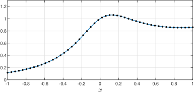
Figure 1: AAA interpolation of $f(x)=e^{x}/\sqrt{1+9x^{2}}$ in $50$ equispaced points in $[-1,1]$. The rational interpolant, of degree $17$, matches $f$ to accuracy $3.3\times 10^{-14}$ at the sample points and $9.6\times 10^{-14}$ on $[-1,1]$.

In this complicated situation we will do our best to elucidate the properties of AAA interpolation. First we compare its performance numerically against that of some existing algorithms for a collection of approximation problems (sections 2 and 3), and then we present certain theoretical considerations (section 4). The final section briefly discusses AAA variants, the effect of noise, and other issues.

Apart from some remarks around Figure 5, we will not describe details of the AAA algorithm, partly because these can be found elsewhere [35] and partly because the essential point here is not AAA per se but just rational approximation. At present, AAA appears to be the best general-purpose rational approximation tool available, but other methods may come along in the future.

2 Existing methods

Many methods have been proposed for interpolation or approximation of equispaced data, and we will not attempt a comprehensive review. We will, however, mention the main categories of methods and choose five specific examples for numerical comparisons. For previous surveys with further references, see [12, 13, 39].

With any interpolant or approximant, there are always the two questions of the form of the approximant and the method of defining or computing it. The main forms that have been advocated are polynomials or piecewise polynomials, Fourier series, rational functions, radial basis functions (RBFs), and various modifications and combinations of these. The methods proposed generally involve mathematically exact interpolation or some version of least-squares approximation. (Ironically, because of conditioning issues, exact interpolants may be less accurate in floating-point arithmetic than least-squares approximations, even at the sample points, let alone in-between.) Almost every method involves a choice of one or two parameters, which usually affect the tradeoff between accuracy and stability and can therefore be interpreted in part as regularization parameters. AAA interpolation may appear at first as an exception to this rule, but a parameter implicitly involved is the tolerance, which in the Chebfun implementation is set by default to $10^{-13}$. We will discuss this further in Section 4.

Polynomial least-squares. Interpolation of $n$ data values by a polynomial of degree $n-1$ leads to exponential instability at a rate $O(2^{n})$, as has been known since Runge in 1901 [41, 44]. Least-squares fitting by a polynomial of degree $d<n-1$, however, is better behaved. To cut off the exponential growth as $n\to\infty$ entirely, $d$ must be restricted to size $O(\sqrt{n}\kern 1.0pt)$ [14, 40], but one can often get away with larger values in practice, and a simple choice is $d\approx n/\gamma$, where $\gamma>1$ is an oversampling ratio. According to equation (4.1) of [39], this cuts the exponential unstable growth rate from $2^{n}$ to $C^{n}$ with

(3) $$C=\left[(1+\alpha)^{1+\alpha}(1-\alpha)^{1-\alpha}\right]^{1/2},\quad\alpha=1/\gamma.$$

For example, $\gamma=2$ yields a growth rate of about $(3^{3/4}/2)^{n}\approx(1.14)^{n}$, which is mild enough to be a good choice in many applications. Our experiments of Figure 2 in the next section use this value $\gamma=2$.

Fourier, polynomial, and RBF extensions. The idea of Fourier extension is to approximate $f$ by a Fourier series tied not to $[-1,1]$ but to a larger domain $[-T,T\kern 1.0pt]$ [9, 16]. The fit is carried out by least-squares or regularized least-squares, often simply by means of the backslash operator in MATLAB, as has been analyzed by Adcock, Huybrechs, and Vaquero [4, 28] and Lyon [34]. A related idea is polynomial extension, in which $f$ is approximated by polynomials expressed in a basis of orthogonal polynomials defined on an interval $[-T,T\kern 1.0pt]$ [5]. A third possibility is RBF extension, in which $f$ is approximated by smooth RBFs whose centers extend outside $[-1,1]$ [24, 37]. In Figure 2 of the next section, we use Fourier extension with $T=2$ and an oversampling ratio of $2$, so that the least-squares matrices have twice as many rows as columns.

Fourier series with corrections. If $f$ is periodic, trigonometric (Fourier) interpolation provides a perfect approximation method: exponentially convergent and stable. In the case of quadrature, this becomes the exponentially convergent trapezoidal rule [46]. For nonperiodic $f$, an attractive idea is to employ a trigonometric fit modified by corrections of one sort or another, often the addition of a polynomial term, designed to mitigate the effect of the implicit discontinuity at the boundary. This idea goes back as far as James Gregory in 1670, before Fourier analysis and even calculus [23]!  The result will not be exponentially convergent, but it can have an algebraic convergence rate of arbitrary order depending on the choice of the corrections, and the rate may improve to super-algebraic if the correction order is taken to increase with $n$. This idea has been applied in many variations, an early example being a method of Eckhoff with precursors he attributes to Krylov and Lanczos [21]. In the “Gregory interpolant” of [29], an interpolant in the form of a sum of a trigonometric term and a polynomial is constructed whose integral equals the result for the Gregory quadrature formula. Fornberg has proposed (for quadrature, not yet approximation) a method of regularized endpoint corrections in which extra parameters are introduced whose amplitudes are then limited by optimization [23]. Figure 2 of the next section shows curves for a least-squares method in which a Fourier series is combined with a polynomial term of degree about $\sqrt{n}$, with an oversampling ratio of about $2$.

Multi-domain methods. Related in spirit to methods involving boundary corrections are methods in which $f$ is approximated by different functions over different subintervals of $[-1,1]$—in the simplest case, a big central interval and two smaller intervals near the ends. For examples see [10, 13, 32, 38].

Splines. Splines, which are piecewise polynomials satisfying certain continuity conditions, take the multi-domain idea further and are an obvious candidate for approximations that will not suffer from Gibbs oscillations at the boundaries. The most familiar case is cubic spline interpolants, where the sample points are nodes separating cubic pieces with continuity of function values and first and second derivatives. Cubic splines (with the standard natural boundary conditions at the ends and not-a-knot conditions one node in from the ends) are one of the methods presented in Figure 2 of the next section.

Mapping. By a conformal map, polynomial approximations can be transformed to other approximations that are more suitable for equispaced interpolation and approximation. The prototypical method in this area was introduced by Kosloff and Tal-Ezer [33], and there is also a connection with prolate spheroidal wave functions [36]. The general conformal mapping point of view was put forward in [27] and in [44, chapter 22]. See also [11].

Gegenbauer reconstruction. Another class of methods has been developed from the point of view of edge detection and elimination of the Gibbs phenomenon in harmonic analysis. For entries into this extensive literature, see [25] and [42].

Explicit regularization methods. Several other methods, often nonlinear, have been proposed involving various strategies of explicit regularization to counter the instability of high-accuracy approximation [6, 8, 17, 47]. We emphasize that even many of the simpler numerical methods implicitly involve regularization introduced by rounding errors, as will be discussed in Section 4.

Floater–Hormann rational interpolation: Chebfun ’equi’. Finally, here is another method involving rational functions. Floater and Hormann introduced a family of degree $n-1$ rational interpolants in barycentric form whose weights can be adjusted to achieve any prescribed order of accuracy [22]. (The AAA method also uses a barycentric representation, but it is an approximant, in principle, not an interpolant, and it is not very closely related to Floater–Hormann approximation.) The method we show in Figure 2 of the next section, due to Klein [26, 31], is based on interpolants whose order of accuracy is adaptively determined via the ’equi’ option of the Chebfun constructor [7, 43].

3 Numerical comparison

As mentioned in the opening paragraph, our interpolation method consists of AAA approximation with its standard tolerance of $10^{-13}$, so long as the approximant that is produced has no “bad poles,” that is, poles in the interval $[-1,1]$. The principal drawback of AAA approximation is that such poles sometimes appear—often with such small residues that they do not contribute meaningfully to the quality of the approximation (in which case they may be called “spurious poles” or “Froissart doublets” [44]). When the original AAA paper [35] was published, a “cleanup” procedure was proposed to address this problem. We are no longer confident that this procedure is very helpful, and instead, we now propose the method of AAA-least squares (AAA-LS) introduced in [18]. Here, if there are any bad poles, these are discarded, and the other poles are retained to form the basis of a linear least-squares fit to find a new rational approximation represented in partial fractions form. For details, see the “if any” block in the AAA part of the code listed in the appendix. Typically this correction makes little difference to accuracy down to levels of $10^{-7}$ or so, but it is often unsuccessful at achieving tighter accuracies than this.

Poles in $[-1,1]$ almost never appear in the approximation of functions $f(x)$ that are complex (a case not illustrated here as it is less common in applications). For real problems, accordingly, another way of avoiding bad poles is to perturb the data by a small, smooth complex function. Overall, however, it must be said that the appearance of unwanted poles in AAA approximants is not yet fully understood, and it seems likely that improvements are in store in this active research area.

Comparing the AAA method against other methods can quickly grow very complicated since most methods have adjustable parameters and there are any number of functions one could apply them to. To keep the discussion under control, the panels of Figure 2 correspond to five functions:

(4) $$f_{A}(x) =\sqrt{1.21-x^{2}}\kern 20.0pt \pm 1.1$$ (branch points at ),

(5) $$f_{B}(x) =\sqrt{0.01+x^{2}} \pm 0.1i$$ (branch points at ),

(6) $$f_{C}(x) =\tanh(5x)$$ (poles on the imaginary axis),

(7) $$f_{D}(x) =\sin(40x)$$ (entire, oscillatory),

(8) $$f_{E}(x) =\exp(-1/x^{2}) C^{\infty}$$ ( but not analytic).

Each panel displays convergence curves for six methods:       Cubic splines,       Polynomial least-squares with oversampling ratio $\gamma=2$,       Fourier extension on $[-2,2]$ with oversampling ratio $\gamma=2$,       Fourier series plus polynomial of degree $\sqrt{n}$ with oversampling ratio $\gamma=2$,       Floater–Hormann rational interpolation: Chebfun ’equi’,       AAA with tolerance $10^{-13}$. For details of the methods, see the code listing in the appendix.

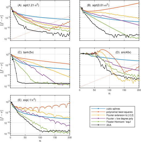
Figure 2: Six approximation methods applied to five smooth functions on $[-1,1]$. In each case the horizontal axis is $n$, the number of sample points, and the vertical axis is $\|f-r\|$, the maximum error over $[-1,1]$. The thicker dot on the AAA curve marks the final value of $n$ at which the rational function is an interpolant rather than just an approximation. The dashed lines in (A) and (D) mark the instability estimate $(1.14)^{n}\varepsilon_{\hbox{\scriptsize\rm machine}}$ from $(\ref{kuijlaars})$ with oversampling ratio $\gamma=2$. The results are discussed in the text, and the code is listed in the appendix.

Many observations can be drawn from Figure 2. The most basic is that AAA consistently appears to be the best of the methods, and is the first to reach accuracy $10^{-10}$ in every case. It is typical for AAA to converge twice as fast as the other methods, and for the test function $f_{C}(x)=\tanh(z)$, whose singularities consist of poles that the AAA approximants readily capture, its superiority is especially striking.

It is worth spelling out the meaning of the AAA convergence curves of Figure 2. Each point on one of these curves corresponds to a rational approximation whose error is $10^{-13}$ or less on the discrete grid (at least if the partial fractions least-squares procedure has not been invoked because of bad poles). For very small $n$, this will be a rational interpolant, of degree $\lceil(n-1)/2\rceil$, with error exactly zero on the grid in principle though nonzero in floating-point arithmetic. In the figure, the last such $n$ is marked by a thicker dot. For most $n$, AAA terminates with a rational approximant of degree less than $\lceil(n-1)/2\rceil$ that matches the data to accuracy $10^{-13}$ on the grid without interpolating exactly. We think of this as a numerical interpolant, since the error on the grid is so small, whereas much larger errors are possible between the grid points. As the grid gets finer, the errors between grid points reduce until the tolerance of $10^{-13}$ is reached all across $[-1,1]$.

Another observation about Figure 2 is that the Floater–Hormann ’equi’ method is very good [7]. Unlike AAA in its pure form, without partial fractions correction, it is guaranteed always to produce an interpolant that is pole-free in $[-1,1]$.

The slowest method to converge is often cubic splines, whose behavior is rock solid algebraic at the fixed rate $\|f-r\|=O(n^{-4})$, assuming $f$ is smooth enough. The convergence of spline approximations could be speeded up by using degrees that increase with $n$ (no doubt at the price of some of that rock solidity).

In panels (A) and (D) of Figure 2, the polynomial least-squares approximations converge at first but eventually diverge exponentially because of unstable amplification of rounding errors. Note that the upward-sloping red curves in these two figures both extrapolate back to about $10^{-16}$, machine precision; the dotted red lines mark the prediction $10^{-16}\times(1.14)^{n}$ from (3) with $\gamma=2$. Before this point, it is interesting to compare the very different initial phases for $f_{A}$, with singularities near $x=\pm 1$, and $f_{B}$, with singularities near $x=0$. Clearly we have initial convergence in the first case and initial divergence in the second, a consequence of Runge’s principle that convergence of polynomial interpolants depends on analyticity near the middle of the interval. The figure for the function $f_{E}$ looks much like that for $f_{B}$.

The Fourier extension method, as a rule, does somewhat better than polynomial least-squares in Figure 2; in certain limits one expects Fourier methods to have an advantage over polynomials of a factor of $\pi/2$ [44, chapter 22]. Perhaps not too much should be read into the precise positions of these curves in the figure, however, as both methods have been implemented with arbitrary choices of parameters that might have been adjusted in various ways.

4 Convergence properties

What can be said in general about AAA approximation of equispaced data? We shall organize the discussion around two questions to be taken up in successive subsections.

• How does the method normally behave?

• How is this behavior consistent with the impossibility theorem?

It would be good to support our observations with theorems guaranteeing the success of the method under appropriate hypotheses, but unfortunately, like most methods of rational approximation, AAA lacks a theoretical foundation.

A key property affecting all of the discussion is that, unlike four of the other five methods of Figure 2 (all but Floater–Hormann ’equi’), AAA approximation is nonlinear. As so often happens in computational mathematics, the nonlinearity is essential to its power, while at the same time leading to analytical challenges. For example, it means that the theory of frames in numerical approximation, as presented in [2, 3, 20], is not directly applicable. A theme of that theory, however, remains important here, which is to distinguish between approximation and sampling. The approximation issue is, how well can rational functions approximate a smooth function $f$ on $[-1,1]$? The sampling issue is, how effectively will an algorithm based on equally spaced samples find these good rational approximations?

Our discussion will make reference to the five example functions $f_{A},\dots,f_{E}$ of Figure 2, which are illustrative of many more experiments we have carried out, and in addition we will consider a sixth function. In any analysis of polynomial approximations on $[-1,1]$, and also in the proof of the impossibility theorem (even though this result is not restricted to polynomial approximations), one encounters functions analytic inside a Bernstein ellipse in the complex plane, which means an ellipse with foci $\pm 1$. We define the amber function (Bernstein means amber in German) by its Chebyshev series

(9) $$A(x)=\sum_{k=0}^{\infty}2^{-k}s_{k}T_{k}(x),$$

where the numbers $s_{k}=\pm 1$ are determined by the binary expansion of $\pi$,

(10) $$\pi=11.00100100001111110110\dots\kern 1.0pt{}_{2},$$

with $s_{k}=1$ when the bit is $1$ and $s_{k}=-1$ when it is $0$. In Chebfun, one can construct $A$ with the commands

              s = dec2bin(floor(2^52*pi));
              c = 2.^(0:-1:-53)’;
              ii = find(s==’0’); c(ii) = -c(ii);
              A = chebfun(c,’coeffs’);

The point of $A(x)$ is that it is analytic in the Bernstein $2$-ellipse but has no further analytic structure beyond that, since the bits of $\pi$ are effectively random. In particular, it is not analytic or meromorphic in any larger region of the $x$-plane. (We believe it has the $2$-ellipse as a natural boundary [30, chap. 4].) Figure 3 sketches $A(x)$ over $[-1,1]$.

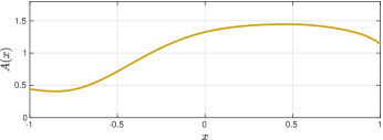
Figure 3: The amber function, a test function constructed to be analytic in the Bernstein $2$-ellipse but not in any larger region of the complex $x$-plane.

Figure 4 is another plot along the lines of Figure 2, but for $A(x)$, and extending to $n=400$ instead of $200$. We are now prepared to examine the properties of AAA interpolation.

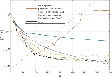
Figure 4: A convergence plot as in Figure 2 for the amber function $A(x)$ of $(\ref{amber})$. Note that for this function, which has no analytic structure beyond analyticity in the Bernstein $2$-ellipse, the AAA and ’equi’ methods perform similarly.

4.1. How does the method normally behave?

We believe the usual behavior of AAA equispaced interpolation is as follows. For small values of $n$, there is a good chance that $f$ will be poorly resolved on the grid, and the initial AAA interpolant will have poles between the grid points in $[-1,1]$. In such cases, as described in the last section, the method switches to a least-squares fit that often produces acceptable accuracy but without outperforming other methods.

As $n$ increases, however, $f$ begins to be resolved, and here rational approximation shows its power. If $f$ happens to be itself rational, like the Runge function $1/(1+25x^{2})$ used for experiments in a number of other papers, AAA may capture it exactly. More typically, $f$ is not rational but, as in the examples of Figure 2, it has analytic structure that rational approximants can exploit. If it is meromorphic, like $\tanh(5x)$, then AAA quickly finds nearby poles and therefore converges at an accelerating rate. Even if it has branch point singularities, rapid convergence still takes place [45].

In this middle phase of rapid convergence of AAA approximation, the errors are many orders of magnitude bigger between the grid points (e.g., $10^{-6}$) than at the grid points ($10^{-13}$). The big errors may be near the endpoints, the pattern familiar in polynomial interpolation since Runge, but they may also be in the interior, as happens for example with approximation of $f(x)=\sqrt{0.01+x^{2}}$. Figure 5 illustrates these two possibilities. Convergence eventually happens because the grid points get closer together and the big errors between them are clamped down.

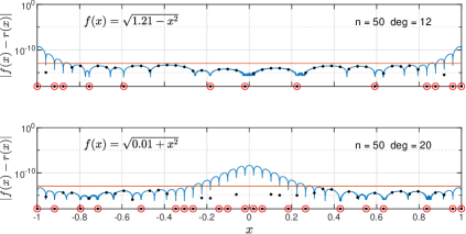
Figure 5: AAA approximation in its mid-phase of rapid convergence at $n=50$ for two different functions $f(x)$. Black dots mark the $n$ sample points, with errors below the AAA relative tolerance level of $10^{-13}$ marked by the red line. The circled black dots are the subset of AAA support points, where the error in principle is $0$ (apart from rounding errors), though it has been artificially plotted at $10^{-18}$. With $f(x)=\sqrt{1.21-x^{2}}$, above, the big errors between sample points are near the boundaries, whereas with $f(x)=\sqrt{0.01+x^{2}}$, below, they are in the interior.

The AAA method does not keep converging for $n\to\infty$, however. Instead, it eventually slows down and is limited by its prescribed relative accuracy, $10^{-13}$ by default. Thus although it gets high accuracy faster than the other methods, in the end it too levels off. To illustrate the significance of the AAA tolerance, Figure 6 repeats the error plots for $f_{C}(x)=\tanh(5x)$ and $f_{D}(x)=\sin(40x)$ for $n=4,8,\dots,200$, but now calculated in 77-digit BigFloat arithmetic using Julia (with the GenericLinearAlgebra package) instead of the usual 16-digit floating point arithmetic. The solid curve shows behavior with tolerance $10^{-13}$ and the blue dots with tolerance $10^{-50}$.

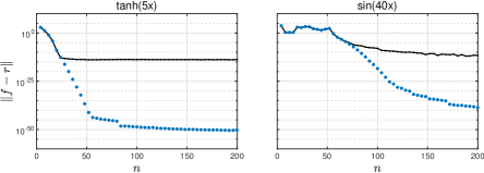
Figure 6: AAA errors for two of the functions of Figure 2 computed in $77$-digit precision with Julia. The solid lines are based on the usual AAA tolerance of $10^{-13}$, and the blue dots are based on tolerance $10^{-50}$. (This computation does not check for poles in $[-1,1]$, which should in principle lead to values $\|f-r\|=\infty$ especially in the early stages of the curves on the right; but here the error is just measured on a $1000$-point equispaced grid.)

The amber function $A(x)$ was constructed to have no hidden analytic structure to be exploited; we think of it as being as far from rational as possible. In Figure 4, this is reflected in the fact that AAA and polynomial approximants converge at approximately the same rate until the latter begins to diverge exponentially. Note also that in Figure 4, unlike the five plots of Figure 2, AAA fails to outperform the Floater–Hormann ’equi’ method. This is consistent with the view that AAA is a robust strategy that exploits analytic structure whereas Floater–Hormann is a robust interpolation strategy that does not exploit analytic structure.

4.2. How is this consistent with the impossibility theorem?

In the introduction we summarized the impossibility theorem of [39] as follows. In approximation of analytic functions from $n$ equispaced samples, exponential convergence as $n\to\infty$ is only possible in tandem with exponential instability; conversely, a stable algorithm can converge at best root-exponentially. The essential reason for this (and the essential construction in the proof of the theorem) can be summarized in a sentence. Some analytic functions are much bigger between the sample points than they are at the sample points; thus high accuracy requires some approximations to be huge. We now explain how the theorem relates to the six numerical methods presented in Figures 2 and 4.

Fourier series plus polynomials, with our choice of polynomial degree $O(\sqrt{n}\kern 1.0pt)$, converge at a root-exponential rate. It it neither exponentially accurate nor exponentially unstable.

The Floater–Hormann ’equi’ interpolant also converges (it appears) at a root exponential rate, for reasons related to its adaptive choice of degree.

Cubic splines converge at a lower rate, just $O(n^{-4})$ for smooth $f$. Again this method is neither exponentially accurate nor exponentially unstable.

Fourier extension also appears to converge root-exponentially, making it, too, neither exponentially accurate nor exponentially unstable.

Polynomial least-squares, however, reveals the hugeness of certain functions. In the terms of the theorem, this is the only one of our methods that appears to be exponentially accurate and exponentially unstable.

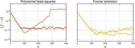
Figure 7: The solid lines repeat the polynomial least-squares (left) and Fourier extension (right) curves of Figure 4. The dots show corresponding results for alternative implementations of each method. On the left, switching to the ill-conditioned monomial basis for polynomial least-squares cuts off the exponential acuracy and also the exponential instability. On the right, switching to the well-conditioned Vandermonde with Arnoldi basis for Fourier extension introduces exponential accuracy and exponential instability.

Our statements about these last two methods, however, come with a big qualification, which is illustrated in Figure 7. In fact, the difference between Fourier extension and polynomial least-squares lies not in their essence but in the fashion in which they are implemented. If you implement either one with a well-conditioned basis, then it is exponentially accurate and exponentially unstable. This is what we have done with the polynomial least-squares method, which uses the well-conditioned basis of Chebyshev polynomials. The Fourier extension method, on the other hand, was implemented with the ill-conditioned basis of complex exponentials $\exp(i\pi kx/2)$. In an ill-conditioned basis like this, high accuracy will require huge coefficient vectors [2, 3, 20], but rounding errors prevent their computation in floating point arithmetic through the mechanism of matrices whose condition numbers are unable to grow bigger than $O((\varepsilon_{\hbox{\scriptsize\rm machine}})^{-1})$. It is these rounding errors that make our implementation of Fourier extension stable. Re-implemented via Vandermonde with Arnoldi [15], as shown in Figure 7, it becomes exponentially accurate and exponentially unstable. Conversely, we can implement polynomial least-squares with the exponentially ill-conditioned monomial basis instead of Chebyshev polynomials. Because of rounding errors, it then loses its its exponential accuracy and its exponential instability, as also shown in Figure 7.

Finally, what about AAA? The experiments suggest it is neither exponentially accurate nor exponentially unstable. Insofar as the impossibility theorem is concerned, there is no inconsistency. Still, what is the mechanism? In Figure 3.1 we have highlighted the last value of $n$ for which AAA interpolates the data. In these and many other examples, that value is very small. Afterwards, AAA favors closer fits to the data over increasing degrees of rational approximation, and this has the familiar effect of oversampling. Yet, owing to its nonlinear nature, AAA is free to vary the oversampling factor—and convergence rates along with it—depending on the data and on the chosen tolerance.

The stability of AAA also stems from the representation of rational functions in barycentric form, which is discussed in the original AAA paper [35].

5 Discussion

Although we have emphasized just the behavior on $[-1,1]$, it is well known that rational approximants have good properties of analytic continuation, beyond the original approximation set. The AAA method certainly partakes of this advantageous behavior. For example, Figure 8 shows the approximation of Figure 1 again ($f(x)=e^{x}/\sqrt{1+9x^{2}}$ sampled at $50$ equispaced points in $[-1,1]$), but now evaluated in the complex plane. There are many digits of accuracy far from the approximation domain $[-1,1]$. This is numerical analytic continuation, and the other methods we have compared against have no such capabilities.

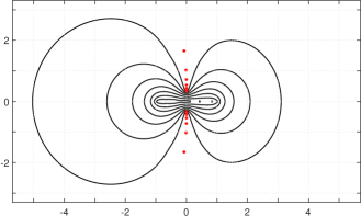
Figure 8: The AAA approximation of Figure 1 extended into the complex plane. The dots are the poles of the rational approximant, and the curves are level curves of the error $|f(z)-r(z)|$ with levels (from outside in) $10^{-2},10^{-4},\dots,10^{-14}$.

Another impressive feature of rational approximation is its ability to handle sampling grids with missing data without much loss of accuracy. A striking illustration of this effect is presented in Figure 2 of [48].

The AAA algorithm, as implemented in Chebfun, has a number of adjustable features. We have bypassed all these, avoiding both the “cleanup” procedure and the Lawson iteration [35] (which is not normally invoked in any case, by default).

One of the drawbacks of AAA approximation is that although it is extremely fast at lower degrees, say, $d<100$, it slows down for higher degrees: the complexity is $O(md^{\kern 0.8pt3})$, where $m$ is the size of the sample set and $d$ is the degree. For most applications, we have in mind a regime of problems with $d<100$. None of the examples shown in this paper come close to this limit. (With the current Chebfun code, one could write for example aaa(F,X,’mmax’,200,’cleanup’,’off’,’lawson’,0).)

Our discussion has assumed that the data $f(x_{k})$ are accurate samples of a smooth function, the only errors being rounding errors down at the relative level of machine precision, around $10^{-16}$. The Chebfun default tolerance of $10^{-13}$ was set with this error level in mind. To handle data contaminated by noise at a higher level $\varepsilon$, we recommend running AAA with its tolerance parameter ’tol’ set to one or two orders of magnitude greater than $\varepsilon$. For unknown noise levels, it should be possible to devise adaptive methods based on apparent convergence rates—detecting the bend in an L-shaped curve—but we have not pursued this. Another approach to dealing with noise in rational approximation is to combine AAA fitting in space with calculations related to Prony’s method in Fourier space, as advocated by Wilber, Damle, and Townsend [48].

Most of the methods we have discussed are linear, but AAA is not. This raises the question, will it do as well for a truly complicated “arbitrary” function as it has done for the functions with relatively simple properties we have examined? As a check of its performance in such a setting, Figure 9 repeats Figure 4, but now for the function $f$ consisting of the sum of all six test functions we have considered: $f_{A},$ $f_{B},$ $f_{C},$ $f_{D},$ $f_{E},$ and $A$. As usual, AAA outperforms the other methods, but blips in the convergence curve at $n=200$ and $264$ highlight that it comes with no guarantees. Both blips correspond to cases where “bad poles” have turned up in the approximation interval $[-1,1]$. These problems are related to rounding errors, as can be confirmed by an implementation in extended precision arithmetic as in Figure 6 or by simply raising the AAA convergence tolerance to $10^{-11}$. It does seem that further research about avoiding unwanted poles in AAA approximation is called for, but fortunately, in a practical setting, such poles are immediately detectable and thus pose no risk of inaccuracy without warning to the user.

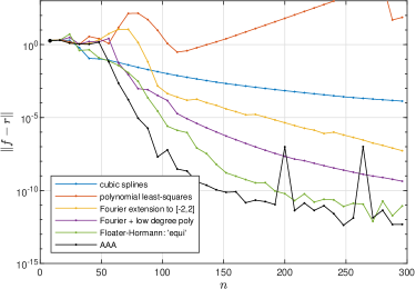
Figure 9: AAA approximation of the function $f(x)$ defined as the sum of all six functions $f_{A},$ $f_{B},$ $f_{C},$ $f_{D},$ $f_{E},$ and $A$ considered in this paper. As usual, AAA mostly outperforms the other methods, but there are blips at $n=200$ and $n=264$ corresponding to poles in the approximation interval $[-1,1]$.

Appendix: MATLAB/Chebfun code for Figure 2

xx = linspace(-1,1,1000)’;
MS = ’markersize’; FS = ’fontsize’; LW = ’linewidth’;
IN = ’interpreter’; LT = ’latex’; warning off
for plt = 1:5
   switch plt
      case 1, s = ’(A)  sqrt(1.21-x^2)’;
      case 2, s = ’(B)  sqrt(0.01+x^2)’;
      case 3, s = ’(C)  tanh(5*x)’;
      case 4, s = ’(D)  sin(40*x)’;
      case 5, s = ’(E)  exp(-1/x^2)’;
   end
   f = inline(vectorize(s(6:end)));
   jplot = 2 - mod(plt,2); iplot = ceil(plt/2);
   axes(’position’,[-.25+.35*jplot 1.04-.32*iplot .3 .27])
   nmax = 200; nn = 4:4:nmax;

% Cubic splines
   nvec = []; errvec = [];
   for n = nn
      X = linspace(-1,1,n)’;
      p = chebfun.spline(X,f(X));
      err = norm(f(xx)-p(xx),inf); nvec = [nvec n]; errvec = [errvec err];
   end
   semilogy(nvec,errvec,’.-’,LW,.5,MS,4), grid on, hold on

% Polynomial least-squares, oversampling ratio 2
   nvec = []; errvec = [];
   for n = nn
      X = linspace(-1,1,n)’;
      A0 = chebpoly(0:n/2); A = A0(X);
      c = A\f(X); AA = A0(xx); pp = AA*c;
      err = norm(f(xx)-pp,inf); nvec = [nvec n]; errvec = [errvec err];
   end
   semilogy(nvec,errvec,’.-’,LW,.5,MS,4), grid on

% Fourier extension on [-2,2], oversampling ratio 2
   nvec = []; errvec = [];
   zz = exp(.5i*pi*xx);
   for n = nn
      X = linspace(-1,1,n)’; Z = exp(.5i*pi*X);
      d = ceil(n/4); c = [real(Z.^(0:d)) imag(Z.^(1:d))]\f(X);
      c = c(1:d+1) - 1i*[0; c(d+2:2*d+1)];
      pp = real((zz.^(0:length(c)-1))*c);
      err = norm(f(xx)-pp,inf); nvec = [nvec n]; errvec = [errvec err];
   end
   semilogy(nvec,errvec,’.-’,LW,.5,MS,4), grid on, hold on

% Fourier plus polynomial of degree sqrt(n), oversampling ratio 2
   nvec = []; errvec = [];
   for n = nn
      degp = round(sqrt(n)) - 1;     % degree of polynomial term
      degp = degp + mod(degp+n+1,2); %   ... with opposite parity to n
      degf = (n-1-degp)/2;
      degf = ceil(degf/2);           % oversampling ratio about 2
      X = linspace(-1,1,n)’;
      C = chebpoly(0:degp);
      A = [cos(pi*(1:degf).*X) sin(pi*(1:degf).*X) C(X)]; c = A\f(X);
      p = @(x) reshape([cos(pi*(1:degf).*x(:)) ...
                        sin(pi*(1:degf).*x(:)) C(x(:))]*c,size(x));
      err = norm(f(xx)-p(xx),inf); nvec = [nvec n]; errvec = [errvec err];
   end
   semilogy(nvec,errvec,’.-’,LW,.5,MS,4), grid on, hold on

% Floater-Hormann rational interpolation: chebfun ’equi’
   nvec = []; errvec = [];
   for n = nn
      X = linspace(-1,1,n)’;
      p = chebfun(f(X),’equi’);
      err = norm(f(xx)-p(xx),inf); nvec = [nvec n]; errvec = [errvec err];
   end
   semilogy(nvec,errvec,’.-’,LW,.5,MS,4), grid on

% AAA
   nvec = []; errvec = []; lastinterp = 0;
   for n = nn
      X = linspace(-1,1,n)’;
      [r,pol] = aaa(f(X),X,’cleanup’,’off’);
      if any(imag(pol)==0 & abs(pol)<1)           % if there are poles in [-1,1],
         pol = pol(imag(pol)~=0 | abs(pol)>1);    % switch to AAA-least squares
         pX = pol.’; for j = 1:length(pol); pX(j) = min(abs(pol(j)-X)); end
         A = [X.^0 pX./(X-pol.’)]; c = A\f(X);
         r = @(x) reshape([x(:).^0 pX./(x(:)-pol.’)]*c, size(x));
      end
      if length(pol) == ceil((n-1)/2), lastinterp = lastinterp+1; end
      err = norm(f(xx)-r(xx),inf);
      nvec = [nvec n]; errvec = [errvec err];
   end
   semilogy(nvec,errvec,’.-k’,LW,.5,MS,4), grid on
   if lastinterp > 0, plot(nvec(lastinterp),errvec(lastinterp),’.k’,MS,8), end

   set(gca,FS,5), axis([0 nmax 1e-16 1e3])
   ylabel(’$\|f-r\|$’,FS,7,IN,LT), xlabel(’$n$’,FS,7,IN,LT)
   if plt < 4, set(gca,’xticklabel’,{}), xlabel(’ ’), end
   if mod(plt,2) == 0, set(gca,’yticklabel’,{}), ylabel(’ ’), end
   if plt == 1 | plt == 4
      plot([0 n],eps*1.14.^[0 n],’:’,’color’,[.85 .325 .098])
   end
   s2 = strrep(s,’*’,’’);
   if plt == 4, text(121,10,s2,FS,6), else text(25,10,s2,FS,6), end
   set(gca,’ytick’,10.^(-15:5:0),’yminorgrid’,’off’), hold off, shg
end
axes(’position’,[.49 .14 .25 .15])
for j = 1:5, plot([0 1],[0 0],’.-’), hold on, end
plot([0 1],[0 0],’.-k’), axis([2 3 2 3]), axis off
legend(’cubic splines’,’polynomial least-squares’,’Fourier extension to [-2,2]’,...
    ’Fourier + low degree poly’,’Floater-Hormann: ’’equi’’’,’AAA’,’location’,...
    ’southeast’,FS,5)
print -depsc testsplt

References

- [1] B. Adcock and D. Huybrechs, On the resolution power of Fourier extensions for oscillatory functions, J. Comput. Appl. Math., 260 (2014), pp. 312–336.
- [2] B. Adcock and D. Huybrechs, Frames and numerical approximation, SIAM Rev., 61 (2019), pp. 443–473.
- [3] B. Adcock and D. Huybrechs, Frames and numerical approximation II: generalized sampling, J. Fourier Anal. Applics., 26 (2020), pp. 1–34.
- [4] B. Adcock, D. Huybrechs, and J. Martín-Vaquero, On the numerical stability of Fourier extensions, Found. Comput. Math., 14 (2014), pp. 635–687.
- [5] B. Adcock and A. Shadrin, Fast and stable approximation of analytic functions from equispaced samples via polynomial frames, arXiv:2110.03755v2, 2022.
- [6] M. Berzins, Adaptive polynomial interpolation on evenly spaced meshes, SIAM Rev., 49 (2007), pp. 604–627.
- [7] L. Bos, Stefano De Marchi, Kai Hormann, and Georges Klein, On the Lebesgue constant of barycentric rational interpolation at equidistant nodes, Numer. Math., 121 (2012), pp. 461–471.
- [8] J. P. Boyd, Defeating the Runge phenomenon for equispaced polynomial interpolation via Tikhonov regularization, Appl. Math. Lett., 20 (2007), pp. 971–975.
- [9] J. P. Boyd, A comparison of numerical algorithms for Fourier extension of the first, second, and third kinds, J. Comput. Phys., 178 (2002), pp. 118–160.
- [10] J. P. Boyd, Exponentially accurate Runge-free approximation of non-periodic functions from samples on an evenly spaced grid, Appl. Math. Lett., 20 (2007), pp. 971–975.
- [11] J. P. Boyd, Quasi-uniform spectral schemes (QUSS), part 1: constructing generalized ellipses for graphical grid generation, Stud. Appl. Math., 136 (2016), pp. 189–213.
- [12] J. P. Boyd and J. R. Ong, Exponentially-convergent strategies for defeating the Runge phenomenon for the approximation of non-periodic functions, part I: single-interval schemes, Commun. Comput. Phys., 5 (2009), pp. 484–497.
- [13] J. P. Boyd and J. R. Ong, Exponentially-convergent strategies for defeating the Runge phenomenon for the approximation of non-periodic functions, part two: multi-interval polynomial schemes and multidomain Chebyshev interpolation, Appl. Numer. Math., 61 (2011), pp. 460–472.
- [14] J. P. Boyd and F. Xu, Divergence (Runge phenomenon) for least-squares polynomial approximation on an equispaced grid and Mock-Chebyshev subset interpolation, Appl. Math. Comput., 210 (2009), pp. 158–168.
- [15] P. D. Brubeck, Y. Nakatsukasa, and L. N. Trefethen, Vandermonde with Arnoldi, SIAM Rev., 63 (2021), pp. 405–415.
- [16] O. P. Bruno, Y. Han, and M. M. Pohlman, Accurate, high-order representation of complex three-dimensional surfaces via Fourier continuation analysis, J. Comput. Phys., 227 (2007), pp. 1094–1125.
- [17] S. Chandrasekaran, K. Jayaraman, J. Moffitt, H. Mhaskar, and S. Pauli, Minimum Sobolev Norm schemes and applications in image processing, Proc. SPIE 7535, (2010), 753507.
- [18] S. Costa and L. N. Trefethen, AAA-least squares rational approximation and solution of Laplace problems, Proceedings 8ECM, to appear.
- [19] T. A. Driscoll, N. Hale, and L. N. Trefethen, Chebfun Guide, Pafnuty Press, Oxford, 2014; see also www.chebfun.org.
- [20] R. J. Duffin and A. C. Schaeffer, A class of nonharmonic Fourier series, Trans. Amer. Math. Soc., 72 (1952), pp. 341–366.
- [21] K. S. Eckhoff, On a high order numerical method for functions with singularities, Math. Comput., 67 (1998), pp. 1063–1087.
- [22] M. S. Floater and K. Hormann, Barycentric rational interpolation with no poles and high rates of approximation, Numer. Math., 107 (2007), pp. 315–331.
- [23] B. Fornberg, Improving the accuracy of the trapezoidal rule, SIAM Rev., 63 (2021), pp. 167–180.
- [24] F. Fryklund, E. Lehto, and A.-K. Tornberg, Partition of unity extension on complex domains, J. Comput. Phys., 375 (2018), pp. 57–79.
- [25] A. Gelb and J. Tanner, Robust reprojection methods for the resolution of the Gibbs phenomenon, Appl. Comput. Harm. Anal., 20 (2006), pp. 3–25.
- [26] S. Güttel and G. Klein, Convergence of linear barycentric rational interpolation for analytic functions, SIAM J. Numer. Anal., 50 (2012), pp. 2560–2580.
- [27] N. Hale and L. N. Trefethen, New quadrature formulas from conformal maps, SIAM J. Numer. Anal., 46 (2008), pp. 930–948.
- [28] D. Huybrechs, Stable high-order quadrature rules with equidistant points, J. Comput. Appl. Math., 231 (2009), pp. 933–947.
- [29] M. Javed and L. N. Trefethen, Euler–Maclaurin and Gregory interpolants, Numer. Math., 132 (2016), pp. 201–216.
- [30] J.-P. Kahane, Some Random Series of Functions, 2nd ed., Cambridge U. Press, 1985.
- [31] G. Klein, Applications of Linear Barycentric Rational Interpolation, PhD thesis, Dept. of Mathematics, U. of Fribourg, 2012.
- [32] G. Klein, An extension of the Floater–Hormann family of barycentric rational interpolants, Math. Comput., 82 (2013), pp. 2273–2292.
- [33] D. Kosloff and H. Tal-Ezer, A modified Chebyshev pseudospectral method with an time step restriction, J. Comput. Phys., 104 (1993), pp. 457–469.
- [34] M. Lyon, A fast algorithm for Fourier continuation, SIAM J. Sci. Comput., 33 (2011), pp. 3241–3260.
- [35] Y. Nakatsukasa, O. Sète, and L. N. Trefethen, The AAA algorithm for rational approximation, SIAM J. Sci. Comput., 40 (2018), pp. A1494–A1522.
- [36] A. Osipov, V. Rokhlin, and H. Xiao, Prolate Spheroidal Wavefunctions of Order Zero: Mathematical Tools for Bandlimited Approximation, Springer, 2013.
- [37] C. Piret, A radial basis function based frames strategy for bypassing the Runge phenomenon, SIAM J. Sci. Comput., 38 (2016), pp. A2262–A2282.
- [38] R. B. Platte and A. Gelb, A hybrid Fourier–Chebyshev method for partial differential equations, J. Sci. Comput., 439 (2009), pp. 244–264.
- [39] R. B. Platte, L. N. Trefethen, and A. B. J. Kuijlaars, Impossibility of fast stable approximation of analytic functions from equispaced samples, SIAM Rev., 53 (2011), pp. 308–318.
- [40] E. A. Rakhmanov, Bounds for polynomials with a unit discrete norm, Ann. of Math., 165 (2007), pp. 55–88.
- [41] C. Runge, Über empirische Funktionen und die Interpolation zwischen äquidistanten Ordinaten, Z. Math. Phys., 46 (1901), pp. 224–243.
- [42] E. Tadmor, Filters, mollifiers and the computation of the Gibbs phenomenon, Acta Numer., 16 (2007), pp. 305–378.
- [43] L. N. Trefethen, Chebfuns from equispaced data, www.chebfun.org/examples/approx/ EquispacedData.html/, 2015.
- [44] L. N. Trefethen, Approximation Theory and Approximation Practice, extended edition, SIAM, Philadelphia, 2019.
- [45] L. N. Trefethen, Y. Nakatsukasa, and J. A. C. Weideman, Exponential node clustering at singularities for rational approximation, quadrature, and PDEs, Numer. Math., 147 (2021), pp. 227–254.
- [46] L. N. Trefethen and J. A. C. Weideman, The exponentially convergent trapezoidal rule, SIAM Rev., 56 (2014), pp. 385–458.
- [47] Q. Wang, P. Moin, and G. Iaccarino, A rational interpolation scheme with superpolynomial rate of convergence, SIAM J. Numer. Anal., 47 (2010), pp. 4073–4097.
- [48] H. Wilber, A. Damle, and A. Townsend, Data-driven algorithms for signal processing with trigonometric rational functions, SIAM J. Sci. Comput., 44 (2022), pp. C185–C209.