Privacy Against Inference Attacks in Vertical Federated Learning

Abstract

Vertical federated learning is considered, where an active party, having access to true class labels, wishes to build a classification model by utilizing more features from a passive party, which has no access to the labels, to improve the model accuracy. In the prediction phase, with logistic regression as the classification model, several inference attack techniques are proposed that the adversary, i.e., the active party, can employ to reconstruct the passive party’s features, regarded as sensitive information. These attacks, which are mainly based on a classical notion of the center of a set, i.e., the Chebyshev center, are shown to be superior to those proposed in the literature. Moreover, several theoretical performance guarantees are provided for the aforementioned attacks. Subsequently, we consider the minimum amount of information that the adversary needs to fully reconstruct the passive party’s features. In particular, it is shown that when the passive party holds one feature, and the adversary is only aware of the signs of the parameters involved, it can perfectly reconstruct that feature when the number of predictions is large enough. Next, as a defense mechanism, several privacy-preserving schemes are proposed that worsen the adversary’s reconstruction attacks, while preserving the benefits that VFL brings to the active party. Finally, experimental results demonstrate the effectiveness of the proposed attacks and the privacy-preserving schemes.

I introduction

To tackle the concerns in the traditional centralized learning, i.e., privacy, storage, and computational complexity, Federated Learning (FL) has been proposed in [1] where machine learning (ML) models are jointly trained by multiple local data owners (i.e., parties), such as smart phones, data centres, etc., without revealing their private data to each other. This approach has gained interest in many real-life applications, such as health systems [2, 3], keyboard prediction [4, 5], and e-commerce [6, 7].

Based on how data is partitioned among participating parties, three variants of FL, which are horizontal, vertical and transfer FL, have been considered. Horizontal FL (HFL) refers to the FL among data owners that share different data records/samples with the same set of features [8], and vertical FL (VFL) is the FL in which parties share common data samples with disjoint set of features [9].

Figure 1 illustrates a digital banking system as an example of a VFL setting, in which two parties are participating, namely, a bank and a FinTech company [10]. The bank wishes to build a binary classification model to approve/disapprove a user’s credit card application by utilizing more features from the Fintech company. In this context, only the bank has access to the class labels in the training and testing datasets, hence named the active party, and the FinTech company that is unaware of the labels is referred to as the passive party.

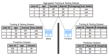
Figure 1: Digital banking as an example of vertical federated learning [10].

Once the model is trained, it can be used to predict the decision (approve/disapprove) on a new credit card application in the prediction dataset. The model outputs, referred to as the prediction outputs or more specifically, the confidence scores, are revealed to the active party that is in charge of making decision. The active party maybe aware or unaware of the passive party’s model parameters, which are, respectively, referred to as the white-box and black-box settings.

As stated in [10], upon the receipt of the prediction outputs, which generally depend on the passive party’s features, a curious active party can perform reconstruction attacks to infer the latter, which are regarded as passive the party’s sensitive information . This privacy leakage in the prediction phase of VFL is the main focus of this paper, and the following contributions are made.

• In the white-box setting, several reconstruction attacks are proposed that outperform those given in [10],[11]. The attacks are motivated by the notion of the Chebyshev center of a convex polytope.

• Theorems 1 and 2 provide theoretical bounds as rigorous guarantees for some of these attacks.

• In the black-box setting, it is shown that when the passive party holds one feature, and the adversary is aware of the signs of the parameters involved, it can still fully reconstruct the passive party’s feature given that the number of predictions is large enough.

• Several privacy-preserving schemes are proposed as a defense technique against reconstruction attacks, which have the advantage of not degrading the benefits that VFL brings to the active party.

The organization of the paper is as follows. In section II, an explanation of the system model under consideration is provided. In section III, the elementary steps that pave the way for the adversary’s attack are elaborated, and the measure by which the performance of the reconstruction attack is evaluated is provided. The analysis and derivations in this paper need some preliminaries from linear algebra and optimization. To make the text as self contained as possible, these have been provided in section IV. The main results of the paper are given in sections V to VIII. In section V, the white-box setting is considered and several attack methods are proposed and evaluated analytically. Section VI deals with the black-box setting and investigates the minimum knowledge the adversary needs to perform a successful attack. In section VII, a privacy-preserving scheme is provided that worsens the adversary’s attacks, while not altering the confidence scores revealed to it. Section VIII is devoted to the experimental evaluation of the results of this paper and comparison to those in the literature. Finally, section IX concludes the paper. To improve the readability, the notation used in this paper is provided next.

Notation. Matrices and vectors are denoted by bold capital (e.g. $\mathbf{A,Q}$) and bold lower case letters (e.g. $\mathbf{b,z}$), respectively. Random variables are denoted by capital letters (e.g. $X$), and their realizations by lower case letters (e.g. $x$). Sets are denoted by capital letters in calligraphic font (e.g. $\mathcal{X},\mathcal{G}$) with the exception of the set of real numbers, i.e., $\mathds{R}$. The cardinality of the finite set $\mathcal{X}$ is denoted by $|\mathcal{X}|$. For a matrix $\mathbf{A}_{m\times k}$, the null space, rank, and nullity are denoted by $\textnormal{Null}(\mathbf{A})$, $\textnormal{rank}(\mathbf{A})$, and $\textnormal{nul}(\mathbf{A})$, respectively, with $\textnormal{rank}(\mathbf{A})+\textnormal{nul}(\mathbf{A})=k$, i.e., the number of columns. The transpose of $\mathbf{A}$ is denoted by $\mathbf{A}^{T}$, and when $m=k$, its trace and determinant are denoted by $\textnormal{Tr}(\mathbf{A})$ and $\textnormal{det}(\mathbf{A})$, respectively. For an integer $n\geq 1$, the terms $\mathbf{I}_{n}$, $\mathbf{1}_{n}$, and $\mathbf{0}_{n}$ denote the $n$-by-$n$ identity matrix, the $n$-dimensional all-one, and all-zero column vectors, respectively, and whenever it is clear from the context, their subscripts are dropped. For two vectors $\mathbf{a,b}$, $\mathbf{a}\geq\mathbf{b}$ means that each element of $\mathbf{a}$ is greater than or equal to the corresponding element of $\mathbf{b}$. The notation $\mathbf{A}\succeq 0$ is used to show that $\mathbf{A}$ is positive semi-definite, and $\mathbf{A}\succeq\mathbf{B}$ is equivalent to $\mathbf{A}-\mathbf{B}\succeq 0$. For integers $m\leq n$, we have the discrete interval $[m:n]\triangleq\{m,m+1,\ldots,n\}$, and the set $[1:n]$ is written in short as $[n]$. $F_{X}(\cdot)$ denotes the cumulative distribution function (CDF) of random variable $X$, whose expectation is denoted by $\mathds{E}[X]=\int xdF_{X}(x)$. In this paper, all the (in)equalities that involve a random variable are in the almost surely (a.s.) sense, i.e., they happen with probability 1. For $\mathbf{x}\in\mathbb{R}^{n}$ and $p\in[1,\infty]$, the $L^{p}$-norm is defined as $\|\mathbf{x}\|_{p}\triangleq(\sum_{i=1}^{n}|x_{i}|^{p})^{\frac{1}{p}},p\in[1,\infty)$, and $\|\mathbf{x}\|_{\infty}\triangleq\max_{i\in[n]}|x_{i}|$. Throughout the paper, $\|\cdot\|$ (i.e., without subscript) refers to the $L^{2}$-norm. The nuclear norm of matrix $\mathbf{A}$ is denoted by $\|\mathbf{A}\|_{*}\triangleq\textnormal{Tr}(\sqrt{\mathbf{A}^{T}\mathbf{A}})$, which is equal to the sum of its singular values. Let $p,q$ be two arbitrary pmfs on $\mathcal{X}$. The Kullback–Leibler divergence from $q$ to $p$ is defined as $D(p||q)\triangleq\sum_{x}p(x)\log_{2}(\frac{p(x)}{q(x)})$, which is also shown as $D(\mathbf{p}||\mathbf{q})$ with $\mathbf{p},\mathbf{q}$ being the corresponding probability vectors of $p,q$, respectively. Likewise, the cross entropy of $q$ relative to $p$ is given by $H(p,q)\triangleq-\sum_{x}p(x)\log q(x)$, which is also shown as $H(\mathbf{p},\mathbf{q})$. Finally, the total variation distance between two probability vectors is $d_{\textnormal{TV}}(\mathbf{p},\mathbf{q})\triangleq\frac{1}{2}\|\mathbf{p}-\mathbf{q}\|_{1}$.

II System model

II-A Machine learning (ML)

An ML model is a function $f_{\mathbf{\theta}}:\mathcal{X}\to\mathcal{Y}$ parameterized by the vector $\mathbf{\theta}$, where $\mathcal{X}$ and $\mathcal{Y}$ denote the input and output spaces, respectively. Supervised classification is considered in this paper, where a labeled training dataset is used to train the model.

Assume that a training dataset $\mathcal{D}_{\textnormal{train}}\triangleq\{(\mathbf{x}_{i},y_{i})|i\in[n]\}$ is given, where each $\mathbf{x}_{i}$ is a $d$-dimensional example/sample and $y_{i}$ denotes its corresponding label. Learning refers to the process of obtaining the parameter vector $\mathbf{\theta}$ in the minimization of a loss function, i.e.,

$$\min_{\mathbf{\theta}}\frac{1}{n}\sum_{i=1}^{n}l(f_{\mathbf{\theta}}(\mathbf{x}_{i}),y_{i})+\omega(\mathbf{\theta}),$$ (1)

where $l(\cdot,\cdot)$ measures the loss of predicting $f_{\mathbf{\theta}}(\mathbf{x}_{i})$, while the true label is $y_{i},i\in[n]$. A regularization term $\omega(\mathbf{\theta})$ can be added to the optimization to avoid overfitting.

Once the model is trained, i.e., $\mathbf{\theta}$ is obtained, it can be used for the prediction of any new sample. In practice, the prediction is (probability) vector-valued, i.e., it is a vector of confidence scores as $\mathbf{c}=(c_{1},c_{2},\ldots,c_{k})^{T}$ with $\sum_{i}c_{i}=1,c_{i}\geq 0,i\in[k]$, where $c_{i}$ denotes the probability that the sample belongs to class $i$, and $k$ denotes the number of classes. Classification can be done by choosing the class that has the highest confidence score.

In this paper, we focus on logistic regression (LR), which can be modelled as

$$\mathbf{c}=\sigma(\mathbf{Wx}+\mathbf{b}),$$ (2)

where $\mathbf{W}$ and $\mathbf{b}$ are the parameters collectively denoted as $\mathbf{\theta}$, and $\sigma(\cdot)$ is the sigmoid or softmax function in the case of binary or multi-class classification, respectively.

II-B Vertical Federated Learning

VFL is a type of ML model training approach in which two or more parties are involved in the training process, such that they hold the same set of samples with disjoint set of features. The main goal in VFL is to train a model in a privacy-preserving manner, i.e., to collaboratively train a model without each party having access to other parties’ features. Typically, the training involves a trusted third party known as the coordinator authority (CA), and it is commonly assumed that only one party has access to the label information in the training and testing datasets. This party is named active and the remaining parties are called passive. Throughout this paper, we assume that only two parties are involved; one is active and the other is passive. The active party is assumed to be honest but curious, i.e., it obeys the protocols exactly, but may try to infer passive party’s features based on the information received. As a result, the active party is referred to as the adversary in this paper.

In the existing VFL frameworks, CA’s main task is to coordinate the learning process once it has been initiated by the active party. During the training, CA receives the intermediate model updates from each party, and after a set of computations, backpropagates each party’s gradient updates, separately and securely. To meet the privacy requirements of parties’ datasets, cryptographic techniques such as secure multi-party computation (SMC) [12] or homomorphic encryption (HE) [13] are used.

Once the global model is trained, upon the request of the active party for a new record prediction, each party computes the results of their model using their own features. CA aggregates these results from all the parties, obtains the prediction (confidence scores), and delivers that to the active party for further action.

As in [10], we assume that the active party has no information about the underlying distribution of the passive party’s features. However, it is assumed that the knowledge about the name, types and range of the features is available to the active party to decide whether to participate in a VFL or not.

III Problem statement

Let $(\mathbf{Y}^{T},\mathbf{X}^{T})^{T}$ denote a random $d_{t}$-dimensional input sample for prediction, where the $(d_{t}-d)$-dimensional $\mathbf{Y}$ and the $d$-dimensional $\mathbf{X}$ correspond to the feature values held by the active and passive parties, respectively. The VFL model under consideration is LR, where the confidence score is given by $\mathbf{c}=\sigma(\mathbf{z})$ with $\mathbf{z}=\mathbb{W}_{act}\mathbf{Y}+\mathbb{W}_{pas}\mathbf{X}+\mathbf{b}$. Denoting the number of classes in the classification task by $k$, $\mathbb{W}_{act}$ (with dimension $k\times(d_{t}-d)$) and $\mathbb{W}_{pas}$ (with dimension $k\times d$) are the model parameters of the active and passive parties, respectively, and $\mathbf{b}$ is the $k$-dimensional bias vector. From the definition of $\sigma(\cdot)$, we have

$$\ln\frac{c_{m+1}}{c_{m}}=z_{m+1}-z_{m},\ m\in[k-1],$$ (3)

where $c_{m},z_{m}$ denote the $m$-th element of $\mathbf{c},\mathbf{z}$, respectively. Define $\mathbf{J}$ as

$$\mathbf{J}\triangleq\begin{bmatrix}-1&1&0&0&\ldots&0\\ 0&-1&1&0&\ldots&0\\ 0&0&-1&1&\ldots&0\\ \vdots&\vdots&\vdots&\vdots&\ddots&\vdots\\ 0&\ldots&\ldots&0&-1&1\end{bmatrix}_{(k-1)\times k},$$ (4)

whose rows are cyclic permutations of the first row with offset equal to the row index$-1$. By multiplying both sides of $\mathbf{z}=\mathbb{W}_{act}\mathbb{Y}+\mathbb{W}_{pas}\mathbb{X}+\mathbb{b}$ with $\mathbf{J}$, and using (3), we get

$$\mathbb{JW}_{pas}\mathbb{X} =\mathbf{Jz}-\mathbb{J}\mathbb{W}_{act}\mathbf{Y}-\mathbf{Jb}$$ (5)

$$=\mathbf{c}^{{}^{\prime}}-\mathbb{J}\mathbb{W}_{act}\mathbf{Y}-\mathbf{Jb},$$ (6)

where $\mathbf{c}^{\prime}$ is a $(k-1)$-dimensional vector whose $m$-th element is $\ln\frac{c_{m+1}}{c_{m}}$. Denoting the RHS of (6) by $\mathbb{b}^{\prime}$, (6) writes in short as $\mathbf{AX}=\mathbf{b}^{\prime}$, where $\mathbf{A}\triangleq\mathbb{JW}_{pas}$.

Remark 1.

It is important to note that the way to obtain a system of linear equations is not unique, but all of them are equivalent in the sense that they result in the same solution space. More specifically, let $\mathbf{R}_{(k-1)\times(k-1)}$ be an invertible matrix, and define $\mathbf{A}_{\textnormal{new}}\triangleq\mathbf{RA}$ and $\mathbf{b}^{\prime}_{\textnormal{new}}\triangleq\mathbf{Rb}^{\prime}$. We have that both $\mathbf{AX}=\mathbf{b}^{\prime}$ and $\mathbf{A}_{\textnormal{new}}\mathbf{X}=\mathbf{b}^{\prime}_{\textnormal{new}}$ are equivalent.

The white-box setting refers to the scenario where the adversary is aware of $(\mathbf{W}_{act},\mathbf{W}_{pas},\mathbf{b})$ and the black-box setting refers to the context in which the adversary is only aware of $\mathbf{W}_{act}$.

Since the active party wishes to reconstruct the passive party’s features, one measure by which the attack performance can be evaluated is the mean square error per feature, i.e.,

$$\textnormal{MSE}=\frac{1}{d}\mathds{E}\left[\|\mathbf{X}-\hat{\mathbf{X}}\|^{2}\right],$$ (7)

where $\hat{\mathbf{X}}$ is the adversary’s estimate. Let $N$ denote the number of predictions. Assuming that these $N$ predictions are carried out in an i.i.d. manner, Law of Large Numbers (LLN) allows to approximate MSE by its empirical value $\frac{1}{Nd}\sum_{i=1}^{N}\|\mathbf{X}_{i}-\hat{\mathbf{X}_{i}}\|^{2}$, since the latter converges almost surely to (7) as $N$ grows. This observation is later used in the experimental results to evaluate the performance of different reconstruction attacks.

IV Preliminaries

Throughout this paper, we are interested in solving a satisfiable system of linear equations, in which the unknowns (features of the passive party) are in the range $[0,1]$. This can be captured by solving for $\mathbf{x}$ in the equation $\mathbf{Ax}=\mathbf{b}$, where $\mathbf{A}\in\mathds{R}^{m\times d}$, $\mathbf{x}\in[0,1]^{d}$, and $\mathbf{b}\in\mathds{R}^{m}$ for some positive integers $m,d$. We are particularly interested in the case when the number of unknowns $d$ is greater than the number of equations $m$. This is a particular case of an indeterminate/under-determined system, where $\mathbf{A}$ does not have full column rank and an infinitude of solutions exists for this linear system. Since the system under consideration is satisfiable, any solution can be written as $\mathbf{A}^{+}\mathbf{b}+(\mathbf{I}_{d}-\mathbf{A}^{+}\mathbf{A})\mathbf{w}$ for some $\mathbf{w}\in\mathds{R}^{d}$, where $\mathbf{A}^{+}$ denotes the pseudoinverse of $\mathbf{A}$ satisfying the Moore-Penrose conditions[14]. One property of pseudoinverse that is useful in the sequel is that if $\mathbf{A}=\mathbf{U\Sigma V}^{T}$ is a singular value decomposition (SVD) of $\mathbf{A}$, then $\mathbf{A}^{+}=\mathbf{V\Sigma}^{+}\mathbf{U}^{T}$, in which $\mathbf{\Sigma}^{+}$ is obtained by taking the reciprocal of each non-zero element on the diagonal of $\mathbf{\Sigma}$, and then transposing the matrix.

For a given pair $(\mathbf{A},\mathbf{b})$, define

$$\mathcal{S}\triangleq\bigg{\{}\mathbf{x}\in\mathds{R}^{d}\bigg{|}\mathbf{A}\mathbf{x}=\mathbf{b}\bigg{\}}\ ,\ \mathcal{S_{F}}\triangleq\bigg{\{}\mathbf{x}\in\mathcal{S}\cap[0,1]^{d}\bigg{\}},$$ (8)

as the solution space and feasible solution space, respectively. Alternatively, by defining

$$\mathcal{W}\triangleq\bigg{\{}\mathbf{w}\in\mathds{R}^{d}\bigg{|}-\mathbf{A}^{+}\mathbf{b}\leq(\mathbf{I}_{d}-\mathbf{A}^{+}\mathbf{A})\mathbf{w}\leq\mathbf{1}_{d}-\mathbf{A}^{+}\mathbf{b}\bigg{\}},$$ (9)

we have

$$\mathcal{S_{F}}=\bigg{\{}(\mathbf{I}_{d}-\mathbf{A}^{+}\mathbf{A})\mathbf{w}+\mathbf{A}^{+}\mathbf{b}\bigg{|}\mathbf{w}\in\mathcal{W}\bigg{\}}.$$ (10)

We have that $\mathcal{W}$ is a closed and bounded convex set defined as an intersection of $2d$ half-spaces. Since $\mathcal{S_{F}}$ is the image of $\mathcal{W}$ under an affine transformation, it is a closed convex polytope in $[0,1]^{d}$.

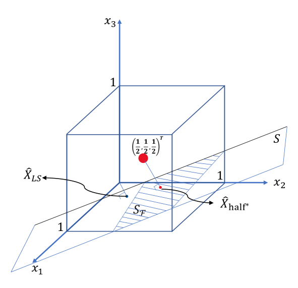
Figure 2: An example with $(m,d)=(1,3)$. The feasible solution space $\mathcal{S_{F}}$ is the intersection of the solution space $\mathcal{S}$, which is denoted by the plane representing $\mathbf{Ax}=\mathbf{b}$, with the hypercube $[0,1]^{3}$. In this example, the minimum-norm point on the solution space, i.e., $\hat{X}_{\textnormal{LS}}$, does not belong to $[0,1]^{3}$.

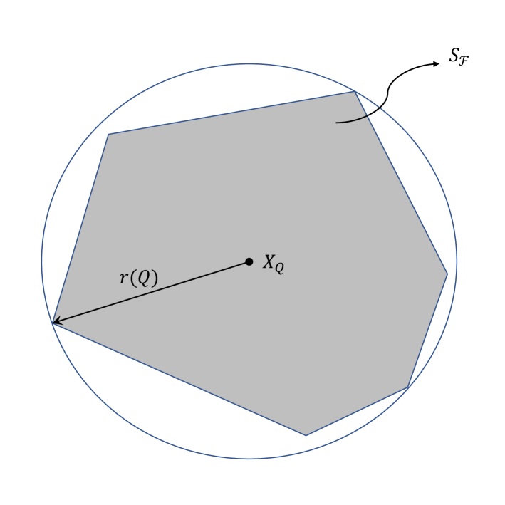
Figure 3: An example of the Chebyshev centre of $\mathcal{Q}$, which is the convex polytope $\mathcal{S_{F}}$ in this paper.

For a general (satisfiable or not) system of linear equations $\mathbf{Cx}=\mathbf{d}$, we have that $\mathbf{C}^{+}\mathbf{d}=\operatorname*{arg\,min}_{\mathbf{x}}\|\mathbf{Cx}-\mathbf{d}\|_{2}$. Moreover, if the system is satisfiable, the quantity $\mathbf{C}^{+}\mathbf{d}$ is the minimum $L^{2}$-norm solution. Therefore, in our problem, we have $\|\mathbf{x}\|_{2}\geq\|\mathbf{A}^{+}\mathbf{b}\|_{2}$ for all $\mathbf{x}\in\mathcal{S}$. Define $\hat{\mathbf{x}}_{\textnormal{LS}}\triangleq\mathbf{A}^{+}\mathbf{b}$, where the subscripts stands for Least Square. It is important to note that $\hat{\mathbf{x}}_{\textnormal{LS}}$ may not necessarily belong to $\mathcal{S_{F}}$, which is our region of interest. A geometrical representation for the case $(m,d)=(1,3)$ is provided in Figure 2. As a result, one can always consider the constrained optimization $\min_{\mathbf{x}}\|\mathbf{A}\mathbf{x}-\mathbf{b}\|_{2}$ with the constraint $\mathbf{0}_{d}\leq\mathbf{x}\leq\mathbf{1}_{d}$ in order to find a feasible solution. We denote any solution obtained in this manner by $\hat{\mathbf{x}}_{\textnormal{CLS}}$, where the subscript stands for Constrained Least Square. In an indeterminate system, in contrast to $\hat{\mathbf{x}}_{\textnormal{LS}}$, $\hat{\mathbf{x}}_{\textnormal{CLS}}$ is not unique, and any point in $\mathcal{S_{F}}$ can be a candidate for $\hat{\mathbf{x}}_{\textnormal{CLS}}$ depending on the initial point of the solver.

Consider this simple example that $x$ is an unknown quantity in the range $[0,1]$ to be estimated and the error in the estimation is measured by the mean square, i.e., $|x-\hat{x}|^{2}$. Obviously, any point in $[0,1]$ can be proposed as an estimate for $x$. However, without any further knowledge about $x$, one can select the center of $[0,1]$, i.e., $\frac{1}{2}$ as an intuitive estimate. The rationale behind this selection is that the maximum error of the estimate $\hat{x}=\frac{1}{2}$, i.e., $\max_{x}|x-\frac{1}{2}|^{2}$ is minimal among all other estimates. In other words, the center minimizes the worst possible estimation error, and hence, it is optimal in the best-worst sense. As mentioned earlier, any element of $\mathcal{S_{F}}$ is a feasible solution of $\mathbf{Ax}=\mathbf{b}$. This calls for a proper definition of the ”center” of $\mathcal{S_{F}}$ as the best-worst solution. This is called the Chebyshev center which is introduced in a general topological context as follows.

Definition 1.

(Chebyshev Center [15]) Let $\mathcal{Q}$ be a bounded subset of a metric space $(\mathcal{X},d)$, where $d$ denotes the distance. A Chebyshev center of $\mathcal{Q}$ is the center of minimal closed ball containing $\mathcal{Q}$, i.e., it is an element $x_{\mathcal{Q}}\in\mathcal{X}$ such that $\sup_{u\in\mathcal{Q}}d(x_{\mathcal{Q}},u)=\inf_{x\in\mathcal{X}}\sup_{u\in\mathcal{Q}}d(x,u)$. The quantity $r(\mathcal{Q})\triangleq\inf_{x\in\mathcal{X}}\sup_{u\in\mathcal{Q}}d(x,u)$ is the Chebyshev radius of $\mathcal{Q}$.

In this paper, the metric space under consideration is $(\mathds{R}^{d},\|\cdot\|_{2})$ for some positive integer $d$, and we have

$$\mathbf{x}_{\mathcal{Q}}\triangleq\operatorname*{arg\,min}_{\hat{\mathbf{x}}\in\mathds{R}^{d}}\max_{\mathbf{x}\in\mathcal{Q}}\|\mathbf{x}-\hat{\mathbf{x}}\|_{2}^{2}.$$ (11)

For example the Chebyshev center of $[0,1]$ in $(\mathds{R},\|\cdot\|_{2})$ is $\frac{1}{2}$, and the Chebyshev center of the ball $\{\mathbf{r}\in\mathds{R}^{2}|\|\mathbf{r}\|\leq 1\}$ in $(\mathds{R}^{2},\|\cdot\|_{2})$ is the origin.

In this paper, the subset of interest, i.e., $\mathcal{Q}$ ($=\mathcal{S_{F}}$), is bounded, closed and convex. In this context, the Chebyshev center of $\mathcal{Q}$ is unique and belongs to $\mathcal{Q}$. Hence, in the argmin in (11), $\hat{\mathbf{x}}\in\mathds{R}^{d}$ can be replaced with $\hat{\mathbf{x}}\in\mathcal{Q}$. An example is provided in Figure 3.

Except for simple cases, computing the Chebyshev center is a computationally complex problem due to the non-convex quadratic inner maximization in (11). When the subset of interest, i.e., $\mathcal{Q}$, can be written as the convex hull of a finite number of points, there are algorithms [16, 17] that can find the Chebyshev center. In this paper, $\mathcal{Q}$($=\mathcal{S_{F}}$) is a convex polytope with a finite number of extreme points (as shown in Figure 2), hence, one can apply these algorithms. However, it is important to note that these extreme points are not given a priori and they need to be found in the first place from the equation $\mathbf{Ax}=\mathbf{b}$. Since the procedure of finding the extreme points of $\mathcal{S_{F}}$ is exponentially complex, it makes sense to seek approximations for the Chebyshev center that can be handled efficiently. Therefore, in this paper, instead of obtaining the exact Chebyshev center of $\mathcal{S_{F}}$, we rely on its approximations. A nice approximation worth mentioning is given in [18], which is in the context of signal processing and is explained in the sequel. This approximation is based on replacing the non-convex inner maximization in (11) by its semidefinite relaxation, and then solving the resulting convex-concave minimax problem. A clear explanation of this method, henceforth named Relaxed Chebyshev Center 1 (RCC1), is needed because it is used as one of the adversary’s attack methods in this paper. Later, in proposition 3, a second relaxation is proposed, which is denoted as RCC2.

The set $\mathcal{Q}$ in [18] is an intersection of $k$ ellipsoids, i.e.,

$$\mathcal{Q}\triangleq\{\mathbf{x}|f_{i}(\mathbf{x})\triangleq\mathbf{x}^{T}\mathbf{Q}_{i}\mathbf{x}+2\mathbf{g}_{i}^{T}\mathbf{x}+t_{i}\leq 0,i\in[k]\},$$ (12)

where $\mathbf{Q}_{i}\succeq 0,\mathbf{g}_{i}\in\mathds{R}^{d},t_{i}\in\mathds{R}$, and the optimization problem is given in (11). Defining $\mathbf{\Delta}\triangleq\mathbf{x}\mathbf{x}^{T}$, the equivalence holds

$$\max_{\mathbf{x}\in\mathcal{Q}}\|\mathbf{x}-\hat{\mathbf{x}}\|^{2}=\max_{(\mathbf{\Delta,x})\in\mathcal{G}}\{\|\hat{\mathbf{x}}\|^{2}-2\hat{\mathbf{x}}^{T}\mathbf{x}+\textnormal{Tr}(\mathbf{\Delta})\},$$ (13)

where $\mathcal{G}=\{(\mathbf{\Delta,x})|\ \textnormal{Tr}(\mathbf{Q}_{i}\mathbf{\Delta})+2\mathbf{g}_{i}^{T}\mathbf{x}+t_{i}\leq 0,i\in[k],\mathbf{\Delta}=\mathbf{x}\mathbf{x}^{T}\}$. By focusing on the right hand side (RHS) of (13) instead of its left hand side (LHS), we are now dealing with the maximization of a concave (linear) function in $(\mathbf{\Delta,x})$. However, the downside is that $\mathcal{G}$ is not convex, in contrast to $\mathcal{Q}$. Here is where the relaxation is done in [18], and the optimization is carried out over a relaxed version of $\mathcal{G}$, i.e.,

$$\mathcal{T}=\{(\mathbf{\Delta,x})|\ \textnormal{Tr}(\mathbf{Q}_{i}\mathbf{\Delta})+2\mathbf{g}_{i}^{T}\mathbf{x}+t_{i}\leq 0,i\in[k],\mathbf{\Delta}\succeq\mathbf{x}\mathbf{x}^{T}\},$$

which is a convex set, and obviously $\mathcal{G}\subset\mathcal{T}$. As a results, RCC1 is the solution to the following minimax problem

$$\min_{\hat{\mathbf{x}}}\max_{(\mathbf{\Delta,x})\in\mathcal{T}}\{\|\hat{\mathbf{x}}\|^{2}-2\hat{\mathbf{x}}^{T}\mathbf{x}+\textnormal{Tr}(\mathbf{\Delta})\}.$$ (14)

Since $\mathcal{T}$ is bounded, and the objective in (14) is convex in $\hat{\mathbf{x}}$ and concave (linear) in $(\mathbf{\Delta,x})$, the order of minimization and maximization can be changed. Knowing that the minimum (over $\hat{\mathbf{x}}$) of the objective function occurs at $\hat{\mathbf{x}}=\mathbf{x}$, (14) reduces to

$$\max_{(\mathbf{\Delta,x})\in\mathcal{T}}\{-\|{\mathbf{x}}\|^{2}+\textnormal{Tr}(\mathbf{\Delta})\},$$

whose objective is concave and the constraints are linear matrrix inequalities, and RCC1 is the $\mathbf{x}$-part of the solution. Since $\mathcal{G}\subset\mathcal{T}$, the radius of the corresponding ball of RCC1 is an upperbound on $r(\mathcal{Q})$, i.e., the Chebyshev radius of $\mathcal{Q}$.

An explicit representation of $\mathbf{x}_{\textnormal{RCC1}}$ is given in [18, Theorem III.1], which is restated here.

$$\mathbf{x}_{\textnormal{RCC1}}=-\bigg{(}\sum_{i=1}^{k}\alpha_{i}\mathbf{Q}_{i}\bigg{)}^{-1}\bigg{(}\sum_{i=1}^{k}\alpha_{i}\mathbf{g}_{i}\bigg{)},$$ (15)

where $(\alpha_{1},\ldots,\alpha_{k})$ is an optimal solution of the following convex problem

$$\min_{\alpha_{i}}\bigg{\{}\bigg{(}\sum_{i=1}^{k}\alpha_{i}\mathbf{g}_{i}\bigg{)}^{T}\bigg{(}\sum_{i=1}^{k}\alpha_{i}\mathbf{Q}_{i}\bigg{)}^{-1}\bigg{(}\sum_{i=1}^{k}\alpha_{i}\mathbf{g}_{i}\bigg{)}-\sum_{i=1}^{k}\alpha_{i}t_{i}\bigg{\}}$$

$$\ \textnormal{S.t.}\ \sum_{i=1}^{k}\alpha_{i}\mathbf{Q}_{i}\succeq\mathbf{I},$$

$$\ \ \ \ \ \ \ \alpha_{i}\geq 0,i\in[k],$$ (16)

which can be cast as a semidefinite program (SDP) and solved by an SDP solver.

It is shown in [18] that similarly to the exact Chebyshev center, $\mathbf{x}_{\textnormal{RCC1}}$ is also unique (due to strict convexity of the $L^{2}$-norm) and it belongs to $\mathcal{Q}$, where the latter follows from the fact that for any $(\mathbf{\Delta}^{\prime},\mathbf{x}^{\prime})\in\mathcal{T}$, we have $\mathbf{x}^{\prime}\in\mathcal{Q}$, which is due to the positive semidefiniteness of $\mathbf{Q}_{i},i\in[k]$.

Finally, suppose that one of the constraints defining the set $\mathcal{Q}$ is a double-sided linear inequality of the form $l\leq\mathbf{a}^{T}\mathbf{x}\leq u$. We can proceed and write this constraint as two constraints, i.e., $\mathbf{a}^{T}\mathbf{x}\leq u$ and $-\mathbf{a}^{T}\mathbf{x}\leq-l$. However, it is shown in [18] that it is better (in the sense of a smaller minimax estimate) to write it in the quadratic form, i.e., $(\mathbf{a}^{T}\mathbf{x}-l)(\mathbf{a}^{T}\mathbf{x}-u)\leq 0$. Although the exact Chebyshev center of $\mathcal{Q}$ does not rely on its specific representation, the RCC1 does, as it is the result of a relaxation of $\mathcal{Q}$. Hence, any constraint of the form $l\leq\mathbf{a}^{T}\mathbf{x}\leq u$ will be replaced by $\mathbf{x}^{T}\mathbf{Q}\mathbf{x}+2\mathbf{g}^{T}\mathbf{x}+t\leq 0$, with $\mathbf{Q}=\mathbf{aa}^{T},\mathbf{g}=-\frac{u+l}{2}\mathbf{a}$, and $t=ul$.

The final discussion in this section is Von Neumann’s trace inequality [19], which is used throughout the paper. It states that for two $n\times n$ (complex) matrices $\mathbf{A,B}$, with singular values $\alpha_{1}\geq\alpha_{2}\geq\ldots\geq\alpha_{n}$ and $\beta_{1}\geq\beta_{2}\geq\ldots\geq\beta_{n}$, respectively, we have

$$|\textnormal{Tr}(\mathbf{AB})|\leq\sum_{i=1}^{n}\alpha_{i}\beta_{i}.$$ (17)

If $\mathbf{A,B}$ are symmetric positive semidefinite matrices with eigenvalues $a_{1}\geq a_{2}\geq\ldots\geq a_{n}$ and $b_{1}\geq b_{2}\geq\ldots\geq b_{n}$, respectively, we have

$$\sum_{i=1}^{n}a_{i}b_{n-i+1}\leq\textnormal{Tr}(\mathbf{AB})\leq\sum_{i=1}^{n}a_{i}b_{i}.$$ (18)

V White-box setting

Let $X\in[0,1]$ be a random variable distributed according to an unknown CDF $F_{X}$. The goal is to find an estimate $\hat{X}$. First, we need the following lemma, which states that when there is no side information available to the estimator, there is no loss of optimality in restricting to the set of deterministic estimates.

Lemma 1.

Any randomized guess is outperformed by its statistical mean, and the performance improvement is equal to the variance of the random guess.

Proof.

Let $\hat{X}$ be a random guess distributed according to a fixed CDF $F_{\hat{X}}$. We have

$$\mathds{E}[(X-\hat{X})^{2}] =\mathds{E}[(X-\mathds{E}[\hat{X}])^{2}]+\textnormal{Var}(\hat{X})$$

$$\geq\mathds{E}[(X-\mathds{E}[\hat{X}])^{2}].$$

Hence, any estimate $\hat{X}\sim F_{\hat{X}}$ is outperformed by the new deterministic estimate $\mathds{E}[\hat{X}]$, whose performance improvement is $\textnormal{Var}(\hat{X})$. ∎

Since the underlying distribution of $X$ is unknown to the estimator, one conventional approach is to consider the best-worst estimator. In other words, the goal of the estimator is to minimize the maximum error, which can be cast as a minimax problem, i.e.,

$$\min_{\hat{x}}\max_{F_{X}}\mathds{E}[(X-\hat{x})^{2}],$$ (19)

where lemma 1 is used in the minimization, i.e., instead of minimizing over $F_{\hat{X}}$, we are minimizing over the singleton $\hat{x}$. Since for any fixed $\hat{x}$, we have $\max_{F_{X}}\mathds{E}[(X-\hat{x})^{2}]=\max_{x\in[0,1]}(x-\hat{x})^{2}$, the best-worst estimation is the solution to

$$\min_{\hat{x}}\max_{x\in[0,1]}(x-\hat{x})^{2},$$ (20)

which is the Chebyshev center of the interval $[0,1]$ in the space $(\mathds{R},\|\cdot\|_{2})$ and it is equal to $\frac{1}{2}$. This implies that with the estimator being blind to the underlying distribution and any possible side information, the best-worst estimate is the Chebyshev center of the support of the random variable, here $[0,1]$.

As one step further, consider that $\mathbf{X}\in[0,1]^{d}$ is a $d$-dimensional random vector distributed according to an unknown CDF $F_{\mathbf{X}}$. Although the estimator is still unaware of $F_{\mathbf{X}}$, this time it has access to the matrix-vector pair $(\mathbf{A},\mathbf{AX})$, and based on this side information, it gives an estimate $\hat{\mathbf{X}}$. This side information refines the prior belief of $\mathbf{X}\in[0,1]^{d}$ to $\mathbf{X}\in\mathcal{S_{F}}$. Similarly to the previous discussion, the best-worst estimator gives the Chebyshev center of $\mathcal{S_{F}}$. As mentioned before, obtaining the exact Chebyshev centre of $\mathcal{S_{F}}$ is computationally difficult, hence, we focus on its approximations. However, prior to the approximation, we start with simple heuristic estimates that bear an intuitive notion of centeredness.

The first scheme in estimating $\mathbf{X}$, is the naive estimate of $\frac{1}{2}\mathbf{1}_{d}$, which is the Chebyshev center of $[0,1]^{d}$. We name this estimate as $\hat{\mathbf{X}}_{\textnormal{half}}=\frac{1}{2}\mathbf{1}_{d}$. We already know that when the only information that we have about $\mathbf{X}$ is that it belongs to $[0,1]^{d}$, then $\hat{\mathbf{X}}_{\textnormal{half}}$ is optimal in the best-worst sense.

The adversary can perform better when the side information $(\mathbf{AX},\mathbf{A})$ is available. A second scheme can be built on top of the previous scheme as follows. The estimator finds a solution in the solution space, i.e., $\mathcal{S}$, that is closest to $\frac{1}{2}\mathbf{1}_{d}$, which is shown in Figure 2. In this scheme, the estimate, named $\hat{\mathbf{X}}_{\textnormal{half}^{*}}$, is given by

$$\hat{\mathbf{X}}_{\textnormal{half}^{*}}\triangleq\operatorname*{arg\,min}_{{\mathbf{x}}\in\mathcal{S}}\|{\mathbf{x}}-\frac{1}{2}\mathbf{1}_{d}\|^{2},$$ (21)

whose explicit representation is provided in the following proposition.

Proposition 1.

We have

$$\hat{\mathbf{X}}_{\textnormal{half}^{*}}=\mathbf{A}^{+}\mathbf{b}+\frac{1}{2}(\mathbf{I}_{d}-\mathbf{A}^{+}\mathbf{A})\mathbf{1}_{d}.$$ (22)

Proof.

For any $\mathbf{x}\in\mathcal{S}$, we have $\mathbf{x}=\mathbf{A}^{+}\mathbf{b}+(\mathbf{I}_{d}-\mathbf{A}^{+}\mathbf{A})\mathbf{w}$ for some $\mathbf{w}\in\mathds{R}^{d}$. Hence,

$$\min_{\hat{\mathbf{x}}\in\mathcal{S}}\|\hat{\mathbf{x}}-\frac{1}{2}\mathbf{1}_{d}\|^{2} =\min_{\mathbf{w}\in\mathds{R}^{d}}\|\mathbf{A}^{+}\mathbf{b}+(\mathbf{I}_{d}-\mathbf{A}^{+}\mathbf{A})\mathbf{w}-\frac{1}{2}\mathbf{1}_{d}\|^{2}$$ (23)

$$=\min_{\mathbf{w}\in\mathds{R}^{d}}\|\mathbf{Cw}-\mathbf{z}\|^{2},$$ (24)

where $\mathbf{C}\triangleq\mathbf{I}_{d}-\mathbf{A}^{+}\mathbf{A}$ and $\mathbf{z}\triangleq\frac{1}{2}\mathbf{1}_{d}-\mathbf{A}^{+}\mathbf{b}$. It is already known that the minimizer in (24) is $\mathbf{w}^{*}=\mathbf{C}^{+}\mathbf{z}$, which results in

$$\hat{\mathbf{X}}_{\textnormal{half}^{*}} =\mathbf{A}^{+}\mathbf{b}+(\mathbf{I}_{d}-\mathbf{A}^{+}\mathbf{A})\mathbf{w}^{*}$$

$$=\mathbf{A}^{+}\mathbf{b}+(\mathbf{I}_{d}-\mathbf{A}^{+}\mathbf{A})(\mathbf{I}_{d}-\mathbf{A}^{+}\mathbf{A})^{+}(\frac{1}{2}\mathbf{1}_{d}-\mathbf{A}^{+}\mathbf{b})$$

$$=\mathbf{A}^{+}\mathbf{b}+(\mathbf{I}_{d}-\mathbf{A}^{+}\mathbf{A})^{2}(\frac{1}{2}\mathbf{1}_{d}-\mathbf{A}^{+}\mathbf{b})$$ (25)

$$=\mathbf{A}^{+}\mathbf{b}+(\mathbf{I}_{d}-\mathbf{A}^{+}\mathbf{A})(\frac{1}{2}\mathbf{1}_{d}-\mathbf{A}^{+}\mathbf{b})$$ (26)

$$=\mathbf{A}^{+}\mathbf{b}+\frac{1}{2}(\mathbf{I}_{d}-\mathbf{A}^{+}\mathbf{A})\mathbf{1}_{d},$$ (27)

where (25) to (27) are justified as follows. Let $\mathbf{A}=\mathbf{U\Sigma V}^{T}$ be an SVD of $\mathbf{A}$. From $\mathbf{A}^{+}=\mathbf{V\Sigma}^{+}\mathbf{U}^{T}$, we get $\mathbf{A}^{+}\mathbf{A}=\mathbf{V\Sigma}^{+}\mathbf{\Sigma V}^{T}$ and $\mathbf{I}-\mathbf{A}^{+}\mathbf{A}=\mathbf{V}(\mathbf{I}-\mathbf{\Sigma}^{+}\mathbf{\Sigma})\mathbf{V}^{T}$. Knowing that $\mathbf{I}-\mathbf{\Sigma}^{+}\mathbf{\Sigma}$ is a diagonal matrix with only 0 and 1 on its diagonal, we get $(\mathbf{I}-\mathbf{\Sigma}^{+}\mathbf{\Sigma})^{+}=\mathbf{I}-\mathbf{\Sigma}^{+}\mathbf{\Sigma}$, and therefore, $(\mathbf{I}-\mathbf{A}^{+}\mathbf{A})^{+}=\mathbf{I}-\mathbf{A}^{+}\mathbf{A}$, which results in (25). Noting that $(\mathbf{I}-\mathbf{A}^{+}\mathbf{A})$ is a projector results in (26). Finally, by noting that $(\mathbf{I}-\mathbf{\Sigma}^{+}\mathbf{\Sigma})\mathbf{\Sigma}^{+}\mathbf{\Sigma}=\mathbf{0}$, we get $(\mathbf{I}-\mathbf{A}^{+}\mathbf{A})\mathbf{A}^{+}\mathbf{b}=\mathbf{0}$, which results in (27). ∎

Thus far, we have considered two simple schemes, i.e., $\hat{\mathbf{X}}_{\textnormal{half}}$ and $\hat{\mathbf{X}}_{\textnormal{half}^{*}}$. In what follows, we investigate two approximations for the Chebyshev center of $\mathcal{S_{F}}$. The exact Chebyshev center of $\mathcal{S_{F}}$ is given by

$$\operatorname*{arg\,min}_{\hat{\mathbf{x}}\in\mathcal{S_{F}}}\max_{\mathbf{x}\in\mathcal{S_{F}}}\|\mathbf{x}-\hat{\mathbf{x}}\|^{2}.$$ (28)

Let $\mathbf{A}=\mathbf{U\Sigma V}^{T}$ be an SVD of $\mathbf{A}$, where the singular values are arranged in a non-increasing order, i.e., $\sigma_{1}\geq\sigma_{2}\geq\sigma_{3}\ldots$. Let $r\triangleq\textnormal{rank}(\mathbf{A})$. Hence, $\textnormal{Null}(\mathbf{A})=\textnormal{Span}\{\mathbf{v}_{r+1},\mathbf{v}_{r+2},\ldots,\mathbf{v}_{d}\}$, which is the span of those right singular vectors that correspond to zero singular values. Define $\mathbf{W}\triangleq[\mathbf{v}_{r+1},\mathbf{v}_{r+2},\ldots,\mathbf{v}_{d}]_{d\times(d-r)}$.

The orthonormal columns of $\mathbf{V}$ can be regarded as a basis for $\mathds{R}^{d}$. Hence, any vector $\mathbf{w}\in\mathds{R}^{d}$ can be written as $\mathbf{w}=\mathbf{Wu}+\mathbf{q}$, where $\mathbf{u}\in\mathds{R}^{d-r},\mathbf{q}\in\mathds{R}^{d}$, and $\mathbf{W}^{T}\mathbf{q}=\mathbf{0}$. With the definition of $\mathbf{W}$, we have

$$\mathbf{I}-\mathbf{A}^{+}\mathbf{A} =\mathbf{V}(\mathbf{I}-\mathbf{\Sigma}^{+}\mathbf{\Sigma})\mathbf{V}^{T}$$

$$=\mathbf{WW}^{T}.$$

Noting that $\mathbf{W}$ has orthonormal columns, we have $\mathbf{W}^{T}\mathbf{W}=\mathbf{I}_{(d-r)}$. Therefore, $\mathcal{S_{F}}$ in (10) can be written as

$$\mathcal{S_{F}}=\{\mathbf{A}^{+}\mathbf{b}+\mathbf{Wu}|\mathbf{u}\in\tilde{\mathcal{S_{F}}}\},\ \tilde{\mathcal{S_{F}}}\triangleq\{\mathbf{u}\in\mathds{R}^{(d-r)}|-\mathbf{A}^{+}\mathbf{b}\leq\mathbf{Wu}\leq\mathbf{1}-\mathbf{A}^{+}\mathbf{b}\}.$$ (29)

Therefore,

$$\min_{\hat{\mathbf{x}}\in\mathcal{S_{F}}}\max_{\mathbf{x}\in\mathcal{S_{F}}}\|\mathbf{x}-\hat{\mathbf{x}}\|^{2} =\min_{\hat{\mathbf{u}}\in\tilde{\mathcal{S_{F}}}}\max_{\mathbf{u}\in\tilde{\mathcal{S_{F}}}}\|\mathbf{A}^{+}\mathbf{b}+\mathbf{Wu}-\mathbf{A}^{+}\mathbf{b}-\mathbf{W\hat{u}}\|^{2}$$

$$=\min_{\hat{\mathbf{u}}\in\tilde{\mathcal{S_{F}}}}\max_{\mathbf{u}\in\tilde{\mathcal{S_{F}}}}\|\mathbf{u}-\mathbf{\hat{u}}\|^{2}.$$ (30)

Denoting the $i$-th row of $\mathbf{W}$ and the $i$-th element of $\mathbf{A}^{+}\mathbf{b}$ by $\mathbf{a}_{i}^{T}$ and $q_{i},i\in[d]$, respectively, the following proposition provides an approximation for the exact Chebyshev center in (28).

Proposition 2.

A relaxed Chebyshev center of $\mathcal{S_{F}}$ is given by

$$\hat{\mathbf{X}}_{\textnormal{RCC1}}=\mathbf{A}^{+}\mathbf{b}-\mathbf{W}\bigg{(}\sum_{i=1}^{d}\alpha_{i}\mathbf{Q}_{i}\bigg{)}^{-1}\bigg{(}\sum_{i=1}^{d}\alpha_{i}\mathbf{g}_{i}\bigg{)},$$ (31)

where $\alpha_{i}$’s are obtained as in (16) with $\mathbf{Q}_{i}=\mathbf{a}_{i}\mathbf{a}_{i}^{T}$, $\mathbf{g}_{i}=(q_{i}-\frac{1}{2})\mathbf{a}_{i}$, and $t_{i}=-q_{i}(1-q_{i})$. Furthermore, $\hat{X}_{\textnormal{RCC1}}$ is unique and it belongs to the set of feasible solution, i.e., $\mathcal{S_{F}}$.

Proof.

The $2d$ linear constraints of $\tilde{\mathcal{S_{F}}}$ are in the form $-q_{i}\leq\mathbf{a}^{T}_{i}\mathbf{u}\leq 1-q_{i}$ for $i\in[d]$. By writing these constraints as their dual quadratic form $\mathbf{u}^{T}\mathbf{Q}_{i}\mathbf{u}+2\mathbf{g}^{T}_{i}\mathbf{u_{i}}+t_{i}\leq 0$, with $\mathbf{Q}_{i}=\mathbf{a}_{i}\mathbf{a}_{i}^{T},\mathbf{g}_{i}=-\frac{1-2q_{i}}{2}\mathbf{a}_{i}$, and $t_{i}=-q_{i}(1-q_{i}),i\in[d]$, and following the approach in [18], which is explained in section IV, $\hat{\mathbf{X}}_{\textnormal{RCC1}}$ is obtained as in (31). Finally, the uniqueness and feasibility of $\hat{\mathbf{X}}_{\textnormal{RCC1}}$ follows from the arguments after (16). ∎

A second relaxation is provided in the following proposition.

Proposition 3.

A relaxed Chebyshev center of $\mathcal{S_{F}}$ is given by

$$\hat{\mathbf{X}}_{\textnormal{RCC2}}=\mathbf{A}^{+}\mathbf{b}+\mathbf{Wu}^{*},$$ (32)

where $\mathbf{u}^{*}$ is the solution of

$$\max_{\mathbf{u}}\ \ \mathbf{1}^{T}\mathbf{Wu}-\|\mathbf{u}\|^{2}$$

$$\ \ \textnormal{S.t.}\ -\mathbf{A}^{+}\mathbf{b}\leq\mathbf{Wu}\leq\mathbf{1}-\mathbf{A}^{+}\mathbf{b}.$$ (33)

Furthermore, $\hat{X}_{\textnormal{RCC2}}$ is unique and it belongs to the set of feasible solution, i.e., $\mathcal{S_{F}}$.

Proof.

The inner maximization in (28) is

$$\max_{\mathbf{x}\in\mathcal{S_{F}}}\|\mathbf{x}-\hat{\mathbf{x}}\|^{2}=\max_{\mathbf{x}\in\mathcal{S_{F}}}\{\|\mathbf{x}\|^{2}-2\mathbf{x}^{T}\hat{\mathbf{x}}+\|\hat{\mathbf{x}}\|^{2}\},$$ (34)

which is a maximization of a convex objective function. As discussed before, one way of relaxing this problem was studied in [18] where the relaxation was over the search space. Here, we propose to directly relax the objective function by making use of the boundedness of $\mathbf{x}$. In other words, since for any $\mathbf{x}\in\mathcal{S_{F}}$, $\mathbf{x}\in[0,1]^{d}$, we have $\|\mathbf{x}\|^{2}\leq\mathbf{1}^{T}\mathbf{x}$. Hence, we can write

$$\min_{\hat{\mathbf{x}}\in\mathcal{S_{F}}}\max_{\mathbf{x}\in\mathcal{S_{F}}}\|\mathbf{x}-\hat{\mathbf{x}}\|^{2} =\min_{\hat{\mathbf{x}}\in\mathcal{S_{F}}}\max_{\mathbf{x}\in\mathcal{S_{F}}}\{\|\mathbf{x}\|^{2}-2\mathbf{x}^{T}\hat{\mathbf{x}}+\|\hat{\mathbf{x}}\|^{2}\}$$

$$\leq\min_{\hat{\mathbf{x}}\in\mathcal{S_{F}}}\max_{\mathbf{x}\in\mathcal{S_{F}}}\{\mathbf{1}^{T}\mathbf{x}-2\mathbf{x}^{T}\hat{\mathbf{x}}+\|\hat{\mathbf{x}}\|^{2}\}$$

$$=\max_{\mathbf{x}\in\mathcal{S_{F}}}\min_{\hat{\mathbf{x}}\in\mathcal{S_{F}}}\{\mathbf{1}^{T}\mathbf{x}-2\mathbf{x}^{T}\hat{\mathbf{x}}+\|\hat{\mathbf{x}}\|^{2}\}$$ (35)

$$=\max_{\mathbf{x}\in\mathcal{S_{F}}}\{\mathbf{1}^{T}\mathbf{x}-\|{\mathbf{x}}\|^{2}\}$$ (36)

$$=\max_{\mathbf{u}\in\tilde{\mathcal{S_{F}}}}\left\{\mathbf{1}^{T}(\mathbf{A}^{+}\mathbf{b}+\mathbf{Wu})-\|\mathbf{A}^{+}\mathbf{b}+\mathbf{Wu}\|^{2}\right\}$$ (37)

$$=\mathbf{1}^{T}\mathbf{A}^{+}\mathbf{b}-\|\mathbf{A}^{+}\mathbf{b}\|^{2}+\max_{\mathbf{u}\in\tilde{\mathcal{S_{F}}}}\{\mathbf{1}^{T}\mathbf{Wu}-\|\mathbf{u}\|^{2}\}$$ (38)

where (35) follows from i) the boundedness of $\mathcal{S_{F}}$, and ii) the concavity (linearity) and convexity of the objective in $\mathbf{x}$ and $\hat{\mathbf{x}}$, respectively. (36) follows from the fact that knowing $\mathbf{x}\in\mathcal{S_{F}}$, $\hat{\mathbf{x}}=\mathbf{x}$ is the minimizer in (35). The RCC2 estimate is the solution of (36). (37) follows from the equivalence given in (29), and denoting the maximizer of (37) by $\mathbf{u}^{*}$, we have $\hat{\mathbf{X}}_{\textnormal{RCC2}}=\mathbf{A}^{+}\mathbf{b}+\mathbf{Wu}^{*}$. In (38), we have used the fact that $\mathbf{W}^{T}\mathbf{A}^{+}\mathbf{A}=0$ and $\mathbf{W}^{T}\mathbf{W}=\mathbf{I}.$

Finally, since the objective of (33) is strictly concave, we have that $\mathbf{u}^{*}$, and hence, $\hat{\mathbf{X}}_{\textnormal{RCC2}}$ are unique. Moreover, due to the constraint in (33), we have $\hat{\mathbf{X}}_{\textnormal{RCC2}}\in\mathcal{S_{F}}$. ∎

Denoting the MSE of a certain estimate $\hat{\mathbf{X}}$ by $\textnormal{MSE}(\hat{\mathbf{X}})$, the following theorem provides a relationship between some of the estimates introduced thus far.

Theorem 1.

The following inequalities hold.

$$\textnormal{MSE}(\hat{\mathbf{X}}_{\textnormal{RCC2}})\leq\textnormal{MSE}(\hat{\mathbf{X}}_{\textnormal{half}^{*}})\leq\textnormal{MSE}(\hat{\mathbf{X}}_{\textnormal{half}}).$$ (39)

Proof.

In order to prove the first inequality, we proceed as follows. The derivative of the objective of (33) with respect to $\mathbf{u}$ is

$$\frac{d}{d\mathbf{u}}(\mathbf{1}^{T}\mathbf{Wu}-\|\mathbf{u}\|^{2})=\mathbf{W}^{T}\mathbf{1}-2\mathbf{u}.$$ (40)

Since the objective in (33) is (strictly) concave in $\mathbf{u}$, by setting $\frac{d}{d\mathbf{u}}(\cdot)=0$, we obtain $\mathbf{u}^{\prime}=\frac{1}{2}\mathbf{W}^{T}\mathbf{1}$ as the maximizer. It is important to note that this $\mathbf{u}^{\prime}$ is not the solution of (33), i.e., $\mathbf{u}^{*}$, in general, as it might not satisfy its constraints. Define $\hat{\mathbf{X}}^{\prime}\triangleq\mathbf{A}^{+}\mathbf{b}+\mathbf{Wu}^{\prime}$. We have

$$\hat{\mathbf{X}}^{\prime} =\mathbf{A}^{+}\mathbf{b}+\frac{1}{2}\mathbf{WW}^{T}\mathbf{1}$$

$$=\mathbf{A}^{+}\mathbf{b}+\frac{1}{2}(\mathbf{I}-\mathbf{A}^{+}\mathbf{A})\mathbf{1}$$ (41)

$$=\hat{\mathbf{X}}_{\textnormal{half}^{*}},$$ (42)

where the equality $\mathbf{I}-\mathbf{A}^{+}\mathbf{A}=\mathbf{WW}^{T}$ follows from the definition of $\mathbf{W}$.

If $\mathbf{u}^{\prime}$ satisfies the constraints of (33), then $\mathbf{u}^{*}=\mathbf{u}^{\prime}$, and $\hat{\mathbf{X}}_{\textnormal{RCC2}}=\hat{\mathbf{X}}_{\textnormal{half}^{*}}$, otherwise, we have that $\mathbf{u}^{*}$ is the point in $\tilde{\mathcal{S_{F}}}$ that is closest to $\mathbf{u}^{\prime}$, and as a result, $\hat{\mathbf{X}}_{\textnormal{RCC2}}$ is the point in $\mathcal{S_{F}}$ that is closest to $\hat{\mathbf{X}}_{\textnormal{half}^{*}}$. This is justified as follows.

$$\mathbf{u}^{*} =\operatorname*{arg\,max}_{\mathbf{u}\in\tilde{\mathcal{S_{F}}}}\{\mathbf{1}^{T}\mathbf{Wu}-\|\mathbf{u}\|^{2}\}$$

$$=\operatorname*{arg\,min}_{\mathbf{u}\in\tilde{\mathcal{S_{F}}}}\{\|\mathbf{u}\|^{2}-\mathbf{1}^{T}\mathbf{Wu}\}$$

$$=\operatorname*{arg\,min}_{\mathbf{u}\in\tilde{\mathcal{S_{F}}}}\{\|\mathbf{u}\|^{2}-\mathbf{1}^{T}\mathbf{Wu}+\|\frac{1}{2}\mathbf{W}^{T}\mathbf{1}\|^{2}\}$$

$$=\operatorname*{arg\,min}_{\mathbf{u}\in\tilde{\mathcal{S_{F}}}}\|\mathbf{u}-\frac{1}{2}\mathbf{W}^{T}\mathbf{1}\|^{2}$$

$$=\operatorname*{arg\,min}_{\mathbf{u}\in\tilde{\mathcal{S_{F}}}}\|\mathbf{u}-\mathbf{u}^{\prime}\|^{2},$$

which results in $\hat{\mathbf{X}}_{\textnormal{RCC2}}=\operatorname*{arg\,min}_{\mathbf{x}\in\mathcal{S_{F}}}\|\mathbf{x}-\hat{\mathbf{X}}_{\textnormal{half}^{*}}\|^{2}$. Hence, we can write

$$(\hat{\mathbf{X}}_{\textnormal{RCC2}}-\hat{\mathbf{X}}_{\textnormal{half}^{*}})^{T}(\mathbf{x}-\hat{\mathbf{X}}_{\textnormal{RCC2}})\geq 0,\ \forall\mathbf{x}\in\mathcal{S_{F}},$$ (43)

which results in the following inequality for $\mathbf{X}\in\mathcal{S_{F}}$

$$\|\mathbf{X}-\hat{\mathbf{X}}_{\textnormal{RCC2}}\|^{2}\leq\|\mathbf{X}-\hat{\mathbf{X}}_{\textnormal{half}^{*}}\|^{2}.$$ (44)

Finally, by taking the expectation of both sides, we obtain

$$\textnormal{MSE}(\hat{\mathbf{X}}_{\textnormal{RCC2}})\leq\textnormal{MSE}(\hat{\mathbf{X}}_{\textnormal{half}^{*}}).$$ (45)

The proof of the second inequality is straightforward. We have $\mathbf{X}-\hat{\mathbf{X}}_{\textnormal{half}}=\mathbf{X}-\hat{\mathbf{X}}_{\textnormal{half}^{*}}+\hat{\mathbf{X}}_{\textnormal{half}^{*}}-\hat{\mathbf{X}}_{\textnormal{half}}$. The proof is concluded by showing that $\mathbf{X}-\hat{\mathbf{X}}_{\textnormal{half}^{*}}$ is orthogonal to $\hat{\mathbf{X}}_{\textnormal{half}^{*}}-\hat{\mathbf{X}}_{\textnormal{half}}$, i.e., $(\mathbf{X}-\hat{\mathbf{X}}_{\textnormal{half}^{*}})^{T}(\hat{\mathbf{X}}_{\textnormal{half}^{*}}-\hat{\mathbf{X}}_{\textnormal{half}})=0$. By noting that $\mathbf{X}$ can be written as $\mathbf{A}^{+}\mathbf{b}+(\mathbf{I}-\mathbf{A}^{+}\mathbf{A})\mathbf{w}$ for some $\mathbf{w}\in\mathds{R}^{d}$, we have

$$\mathbf{X}-\hat{\mathbf{X}}_{\textnormal{half}^{*}} =(\mathbf{I}-\mathbf{A}^{+}\mathbf{A})(\mathbf{w}-\frac{1}{2}\mathbf{1})$$ (46)

$$\hat{\mathbf{X}}_{\textnormal{half}^{*}}-\hat{\mathbf{X}}_{\textnormal{half}} =\mathbf{A}^{+}\mathbf{A}(\mathbf{X}-\frac{1}{2}\mathbf{1}).$$ (47)

Knowing that $(\mathbf{I}-\mathbf{A}^{+}\mathbf{A})\mathbf{A}^{+}\mathbf{A}=0$ proves the orthogonality of the LHS of (46) and (47). Hence, we have

$$\|\mathbf{X}-\hat{\mathbf{X}}_{\textnormal{half}}\|^{2} =\|\mathbf{X}-\hat{\mathbf{X}}_{\textnormal{half}^{*}}\|^{2}+\|\hat{\mathbf{X}}_{\textnormal{half}^{*}}-\hat{\mathbf{X}}_{\textnormal{half}}\|^{2}$$

$$\geq\|\mathbf{X}-\hat{\mathbf{X}}_{\textnormal{half}^{*}}\|^{2},$$ (48)

and by taking the expectation, we get

$$\textnormal{MSE}(\hat{\mathbf{X}}_{\textnormal{half}^{*}})\leq\textnormal{MSE}(\hat{\mathbf{X}}_{\textnormal{half}}).$$ (49)

∎

Remark 2.

(An alternative characterization of RCC2) In (21), $\hat{\mathbf{X}}_{\textnormal{half}^{*}}$ is defined as the point in the solution space, i.e., $\mathcal{S}$, that is closest to $\frac{1}{2}\mathbf{1}_{d}$. Interestingly, we observe that $\hat{\mathbf{X}}_{\textnormal{RCC2}}$, which is independently defined as the second relaxation of the Chebyshev center of $\mathcal{S_{F}}$, can be interpreted in a similar way: it is the point in the feasible solution space $\mathcal{S_{F}}$ that is closest to $\frac{1}{2}\mathbf{1}_{d}$, which is justified as follows.

$$\operatorname*{arg\,min}_{{\mathbf{x}}\in\mathcal{S_{F}}}\|{\mathbf{x}}-\frac{1}{2}\mathbf{1}_{d}\|^{2} =\mathbf{A}^{+}\mathbf{b}+\mathbf{W}\left(\operatorname*{arg\,min}_{\mathbf{u}\in\tilde{\mathcal{S_{F}}}}\|\mathbf{A}^{+}\mathbf{b}+\mathbf{Wu}-\frac{1}{2}\mathbf{1}_{d}\|^{2}\right)$$

$$=\mathbf{A}^{+}\mathbf{b}+\mathbf{W}\left(\operatorname*{arg\,min}_{\mathbf{u}\in\tilde{\mathcal{S_{F}}}}\left\{\|\mathbf{Wu}\|^{2}+2\mathbf{u}^{T}\mathbf{W}^{T}(\mathbf{A}^{+}b-\frac{1}{2}\mathbf{1}_{d})+\|\mathbf{A}^{+}b-\frac{1}{2}\mathbf{1}_{d}\|^{2}\right\}\right)$$

$$=\mathbf{A}^{+}\mathbf{b}+\mathbf{W}\left(\operatorname*{arg\,min}_{\mathbf{u}\in\tilde{\mathcal{S_{F}}}}\left\{\|\mathbf{u}\|^{2}-\mathbf{1}^{T}\mathbf{Wu}\right\}\right)$$

$$=\mathbf{A}^{+}\mathbf{b}+\mathbf{W}\left(\operatorname*{arg\,max}_{\mathbf{u}\in\tilde{\mathcal{S_{F}}}}\left\{\mathbf{1}^{T}\mathbf{Wu}-\|\mathbf{u}\|^{2}\right\}\right),$$

which is the same as (32).

Let $\mathbf{z}$ be an arbitrary vector in $\mathds{R}^{d}$ and define $\mathbf{K}_{\mathbf{z}}\triangleq\mathds{E}[(\mathbf{X}-\mathbf{z})(\mathbf{X}-\mathbf{z})^{T}]$. Define $\mathbf{\mu}\triangleq\mathds{E}[\mathbf{X}]$. In particular, $\mathbf{K}_{\mathbf{0}}$ and $\mathbf{K}_{\mathbf{\mu}}$ denote the correlation and covariance matrices of $\mathbf{X}$, respectively.

Theorem 2.

The following relationships hold.

$$\frac{1}{d}\sum_{i=\textnormal{rank}(\mathbf{A})+1}^{d}\lambda_{i}\leq\textnormal{MSE}(\hat{\mathbf{X}}_{\textnormal{LS}}) =\frac{\textnormal{Tr}\left((\mathbf{I}-\mathbf{A}^{+}\mathbf{A})\mathbf{K}_{\mathbf{0}}\right)}{d}\leq\frac{1}{d}\sum_{i=1}^{\textnormal{nul}(\mathbf{A})}\lambda_{i}$$ (50)

$$\frac{1}{d}\sum_{i=\textnormal{rank}(\mathbf{A})+1}^{d}\gamma_{i}\leq\textnormal{MSE}(\hat{\mathbf{X}}_{\textnormal{half}^{*}}) =\frac{\textnormal{Tr}\left((\mathbf{I}-\mathbf{A}^{+}\mathbf{A})\mathbf{K}_{\frac{1}{2}\mathbf{1}}\right)}{d}\leq\frac{1}{d}\sum_{i=1}^{\textnormal{nul}(\mathbf{A})}\gamma_{i}$$ (51)

$$\textnormal{MSE}(\hat{\mathbf{X}}_{\textnormal{LS}})\ ,\ \textnormal{MSE}(\hat{\mathbf{X}}_{\textnormal{half}^{*}}) \geq\frac{\textnormal{Tr}\left((\mathbf{I}-\mathbf{A}^{+}\mathbf{A})\mathbf{K}_{\mathbf{\mu}}\right)}{d},$$ (52)

where $\lambda_{1}\geq\lambda_{2}\geq\ldots\geq\lambda_{d}$ and $\gamma_{1}\geq\gamma_{2}\geq\ldots\geq\gamma_{d}$ are, respectively, the eigenvalues of $\mathbf{K}_{\mathbf{0}}$ and $\mathbf{K}_{\frac{1}{2}\mathbf{1}}$ arranged in a non-increasing order. We also adopt the convention that $\sum_{i=1}^{0}(\cdot)_{i},\sum_{i=d+1}^{d}(\cdot)_{i}\triangleq 0$.

Proof.

We have

$$\textnormal{MSE}(\hat{\mathbf{X}}_{\textnormal{LS}}) =\frac{1}{d}\mathds{E}[\|\mathbf{X}-\hat{\mathbf{X}}_{\textnormal{LS}}\|^{2}]$$

$$=\frac{1}{d}\mathds{E}[\|\mathbf{X}-\mathbf{A}^{+}\mathbf{b}\|^{2}]$$

$$=\frac{1}{d}\mathds{E}[\|\mathbf{X}-\mathbf{A}^{+}\mathbf{A}\mathbf{X}\|^{2}]$$

$$=\frac{1}{d}\mathds{E}[\|(\mathbf{I}-\mathbf{A}^{+}\mathbf{A})\mathbf{X}\|^{2}]$$

$$=\frac{1}{d}\mathds{E}[\textnormal{Tr}\left((\mathbf{I}-\mathbf{A}^{+}\mathbf{A})\mathbf{XX}^{T}(\mathbf{I}-\mathbf{A}^{+}\mathbf{A})^{T}\right)]$$ (53)

$$=\frac{1}{d}\mathds{E}[\textnormal{Tr}\left((\mathbf{I}-\mathbf{A}^{+}\mathbf{A})\mathbf{XX}^{T}\right)]$$ (54)

$$=\frac{1}{d}\textnormal{Tr}\left((\mathbf{I}-\mathbf{A}^{+}\mathbf{A})\mathbf{K}_{\mathbf{0}}\right),$$ (55)

where (53) follows from having $\|\mathbf{a}\|^{2}=\textnormal{Tr}(\mathbf{aa}^{T})$ for an arbitrary vector $\mathbf{a}$. In (54), we use the invariance of trace under cyclic permutation (in particular $\textnormal{Tr}(\mathbf{AB})=\textnormal{Tr}(\mathbf{BA})$) and the fact that $\mathbf{I}-\mathbf{A}^{+}\mathbf{A}$ is an orthogonal projection, i.e., it is symmetric and $(\mathbf{I}-\mathbf{A}^{+}\mathbf{A})^{2}=\mathbf{I}-\mathbf{A}^{+}\mathbf{A}$. By pushing the expectation inside the trace in (54), which is due to the linearity of the trace operator, (55) is obtained.

Similarly, we have

$$\textnormal{MSE}(\hat{\mathbf{X}}_{\textnormal{half}^{*}}) =\frac{1}{d}\mathds{E}[\|\mathbf{X}-\hat{\mathbf{X}}_{\textnormal{half}^{*}}\|^{2}]$$

$$=\frac{1}{d}\mathds{E}[\|\mathbf{X}-\mathbf{A}^{+}\mathbf{b}-\frac{1}{2}(\mathbf{I}-\mathbf{A}^{+}\mathbf{A})\mathbf{1}\|^{2}]$$

$$=\frac{1}{d}\mathds{E}[\|\mathbf{X}-\mathbf{A}^{+}\mathbf{A}\mathbf{X}-\frac{1}{2}(\mathbf{I}-\mathbf{A}^{+}\mathbf{A})\mathbf{1}\|^{2}]$$

$$=\frac{1}{d}\mathds{E}[\|(\mathbf{I}-\mathbf{A}^{+}\mathbf{A})(\mathbf{X}-\frac{1}{2}\mathbf{1})\|^{2}]$$

$$=\frac{1}{d}\mathds{E}\bigg{[}\textnormal{Tr}\left((\mathbf{I}-\mathbf{A}^{+}\mathbf{A})(\mathbf{X}-\frac{1}{2}\mathbf{1})(\mathbf{X}-\frac{1}{2}\mathbf{1})^{T}(\mathbf{I}-\mathbf{A}^{+}\mathbf{A})^{T}\right)\bigg{]}$$

$$=\frac{1}{d}\mathds{E}\bigg{[}\textnormal{Tr}\left((\mathbf{I}-\mathbf{A}^{+}\mathbf{A})(\mathbf{X}-\frac{1}{2}\mathbf{1})(\mathbf{X}-\frac{1}{2}\mathbf{1})^{T}\right)\bigg{]}$$

$$=\frac{1}{d}\textnormal{Tr}\left((\mathbf{I}-\mathbf{A}^{+}\mathbf{A})\mathbf{K}_{\frac{1}{2}\mathbf{1}}\right).$$

Hence, the equalities in (50) and (51) are proved.

Fix an arbitrary $\mathbf{z}\in\mathds{R}^{d}$, which results in $\mathbf{K}_{\mathbf{z}}$ with eigenvalues denoted by $s_{1}\geq s_{2}\geq\ldots\geq s_{d}$. By applying Von Neumann’s trace inequality, we have

$$\sum_{i=\textnormal{rank}(\mathbf{A})+1}^{d}s_{i}\leq\textnormal{Tr}\left((\mathbf{I}-\mathbf{A}^{+}\mathbf{A})\mathbf{K}_{\mathbf{z}}\right)\leq\sum_{i=1}^{\textnormal{nul}(\mathbf{A})}s_{i},$$ (56)

which follows from the fact that both $\mathbf{K}_{\mathbf{z}}$ and $\mathbf{I}-\mathbf{A}^{+}\mathbf{A}$ are symmetric positive semidefinite matrices and the latter has $\textnormal{nul}(\mathbf{A})$ 1’s and $\textnormal{rank}(\mathbf{A})$ 0’s as eigenvalues. By replacing $\mathbf{z}$ with $\mathbf{0}$ or $\frac{1}{2}\mathbf{1}$, the upper and lower bounds in (50) or (51) are obtained.

For a fixed $\mathbf{z}$, we have

$$\textnormal{Tr}\left((\mathbf{I}-\mathbf{A}^{+}\mathbf{A})\mathbf{K}_{\mathbf{z}}\right)-\textnormal{Tr}\left((\mathbf{I}-\mathbf{A}^{+}\mathbf{A})\mathbf{K}_{\mathbf{\mu}}\right) =\textnormal{Tr}\left((\mathbf{I}-\mathbf{A}^{+}\mathbf{A})(\mathbf{K}_{\mathbf{z}}-\mathbf{K}_{\mathbf{\mu}})\right)$$

$$=\textnormal{Tr}\left((\mathbf{I}-\mathbf{A}^{+}\mathbf{A})(\mathbf{z}-\mathbf{\mu})(\mathbf{z}-\mathbf{\mu})^{T}\right)$$

$$=\textnormal{Tr}\left((\mathbf{z}-\mathbf{\mu})^{T}(\mathbf{I}-\mathbf{A}^{+}\mathbf{A})(\mathbf{z}-\mathbf{\mu})\right)$$

$$=(\mathbf{z}-\mathbf{\mu})^{T}(\mathbf{I}-\mathbf{A}^{+}\mathbf{A})(\mathbf{z}-\mathbf{\mu})$$

$$\geq 0,$$ (57)

where (57) follows from the positive semidefiniteness of $\mathbf{I}-\mathbf{A}^{+}\mathbf{A}$. Replacing $\mathbf{z}$ with $\mathbf{0}$ or $\frac{1}{2}\mathbf{1}$ results in (52). ∎

Remark 3.

From Theorem 2, the passive party can obtain the MSE of the attacks $\hat{\mathbf{X}}_{\textnormal{LS}}$ and $\hat{\mathbf{X}}_{\textnormal{half}^{*}}$ as closed form solutions. It is important to note that in this context, this is still possible although the passive party is unaware of the active party’s model parameters and the confidence scores it receives. We also note that according to remark 1, although the adversary has multiple ways to obtain a system of linear equations, all of them are equivalent. As a result, the passive party can assume that the adversary has obtained this system in a particular way, and obtain the MSE. In other words, regardless of whether the adversary is dealing with $\mathbf{AX}=\mathbf{b}$ or $\mathbf{A}_{\textnormal{new}}\mathbf{X}=\mathbf{b}_{\textnormal{new}}$, with $\mathbf{A}_{\textnormal{new}}=\mathbf{RA}$ and $\mathbf{b}_{new}=\mathbf{Rb}$ for arbitrary invertible $\mathbf{R}$, we have $(\mathbf{I}-\mathbf{A}^{+}\mathbf{A})=(\mathbf{I}-\mathbf{A}_{\textnormal{new}}^{+}\mathbf{A}_{\textnormal{new}})$, which results from i) $\mathbf{R}$ is invertible and ii) $\mathbf{A}$ has linearly independent rows, and hence $(\mathbf{RA})^{+}=\mathbf{A}^{+}\mathbf{R}^{+}=\mathbf{A}^{+}\mathbf{R}^{-1}$.

Remark 4.

In many practical scenarios, we have that $\mathbf{A}$ is either full column or full row rank, which results in $\textnormal{rank}(\mathbf{A})=\min\{k-1,d\}$ (and hence $\textnormal{nul}(\mathbf{A})=\max\{d-k+1,0\}$), where $k$ denotes the number of classes. In this context, the importance of the lower and upper bounds in (50) and (51) is that the passive party can calculate them prior to the training, which can be carried out by calculating the eigenvalues of $\mathbf{K}_{\mathbf{0}}$ and $\mathbf{K}_{\frac{1}{2}\mathbf{1}}$.

Remark 5.

The attack schemes proposed in this section are applied per prediction, i.e., an estimate is obtained after the receipt of the confidence scores for each sample in the prediction set. It is easy to verify that these attacks result in the same performance if applied on multiple predictions. More specifically, assuming that there are $N$ predictions, the resulting system of linear equations is $\mathbf{AX}=\mathbf{b}$, in which $\mathbf{X}$ is an $Nd$-dimensional vector obtained as the concatenation of $N$ $d$-dimensional vectors, $\mathbf{A}$ is $N(k-1)\times Nd$-dimensional, and $\mathbf{b}$ is $N(k-1)$-dimensional. Nonetheless, all the attack methods discussed, do not improve by being applied on multiple predictions.

VI Black-box setting

A relaxed version of the black-box setting is considered in [11], in which the adversary is aware of some auxiliary data, i.e., the passive party’s features for some sample IDs, and based on these auxiliary data, the adversary estimates the passive party’s model parameters. Once this estimate is obtained, any reconstruction attack in the white-box setting can be applied by regarding this estimate as the true model parameters. Needless to say that all the proposed attacks in the previous section of this paper can be applied in this way. However, the real black-box setting in which the adversary cannot have access to auxiliary data remains open. In what follows, we investigate this problem under specific circumstances.

Here, we assume that the passive party has only one feature denoted by $X_{i}\in[0,1],i\in[N]$, corresponding to $N$ predictions. We assume that $(X_{1},X_{2},\ldots,X_{N})$ are i.i.d. according to an unknown CDF $F_{X}$. In the black-box setting, the adversary observes $v_{i}=\omega X_{i}+b,i\in[N]$, where $\omega$ ($\neq 0$) and $b$ are unknown. This is a specific case of (6), where $d=1$. A question that arises here is : How is the performance of the adversary affected by the lack of knowledge about $\omega,b$? In other words, what (minimal) knowledge about $\omega,b$ is sufficient for the adversary in order to perform a successful reconstruction attack in estimating $(X_{1},X_{2},\ldots,X_{N})$? In what follows, it is shown that in certain scenarios, this lack of knowledge has a vanishing effect given that $N$ is large enough.

Lemma 2.

Assume that $(X_{1},X_{2},\ldots,X_{N})$ are i.i.d. according to an unknown CDF $F_{X}$, where $X_{i}\in[0,1],i\in[N]$. Fix an arbitrary $\epsilon\in(0,1)$. We have

$$\lim_{N\to\infty}\textnormal{Pr}\left\{\max_{i\in[N]}X_{i}\leq 1-\epsilon\right\} =0$$

$$\lim_{N\to\infty}\textnormal{Pr}\left\{\min_{i\in[N]}X_{i}\geq\epsilon\right\} =0.$$ (58)

In other words $\max_{i\in[N]}X_{i}$ and $\min_{i\in[N]}X_{i}$ converge in probability to 1 and 0, respectively.

Proof.

We have

$$\lim_{N\to\infty}\textnormal{Pr}\left\{\max_{i\in[N]}X_{i}\leq 1-\epsilon\right\} =\lim_{N\to\infty}\textnormal{Pr}\left\{X_{i}\leq 1-\epsilon,\ \forall i\in[N]\right\}$$

$$=\lim_{N\to\infty}\bigg{(}\textnormal{Pr}\{X_{1}\leq 1-\epsilon\}\bigg{)}^{N}$$ (59)

$$=\lim_{N\to\infty}(F_{X}(1-\epsilon))^{N}$$

$$=0,$$ (60)

and

$$\lim_{N\to\infty}\textnormal{Pr}\left\{\min_{i\in[N]}X_{i}\geq\epsilon\right\} =\lim_{N\to\infty}\textnormal{Pr}\left\{X_{i}\geq\epsilon,\ \forall i\in[N]\right\}$$

$$=\lim_{N\to\infty}\bigg{(}\textnormal{Pr}\{X_{1}\geq\epsilon\}\bigg{)}^{N}$$ (61)

$$=\lim_{N\to\infty}\left(1-\lim_{t\to\epsilon^{-}}F_{X}(t)\right)^{N}$$ (62)

$$=0,$$ (63)

where (59) and (61) are due to the assumption that $X_{i}$’s are i.i.d., and (62) results from the identities $\textnormal{Pr}\{X_{1}\geq\epsilon\}=1-\textnormal{Pr}\{X_{1}<\epsilon\}$ and $\textnormal{Pr}\{X_{1}<\epsilon\}=\lim_{t\to\epsilon^{-}}F_{X}(t)$. Since we are assuming that $X_{i}\in[0,1],\forall i\in[N]$, we have that for any $\alpha\in(0,1)$, $0<F_{X}(\alpha)<1$, since otherwise, the region $[0,1]$ could have been modified accordingly. This results in (60) and (63). ∎

The adversary observes $v_{i}$’s and the problem is divided into three cases as follows.

VI-A Case 1 : $b=0$

In this case, the observations of the adversary are $v_{i}=\omega X_{i},i\in[N]$. The adversary finds the maximum of $|v_{i}|$ and estimates that the feature in charge of generating this value is 1. In other words, let $M\triangleq\operatorname*{arg\,max}_{i\in[N]}|v_{i}|$, and the adversary sets $\hat{X}_{M}=1$. The rationale behind this estimation is that if $N$ is large enough, we are expecting $X_{M}$ to be close to 1 by lemma 2. By design, we have that $\frac{X_{i}}{X_{M}}=\frac{v_{i}}{v_{M}},\forall i\in[N]$. Therefore, it makes sense to set

$$\hat{X}_{i}=\frac{v_{i}}{v_{M}}\hat{X}_{M}=\frac{v_{i}}{v_{M}},\forall i\in[N].$$ (64)

With these estimates, we can write the empirical MSE as

$$\frac{1}{N}\sum_{i=1}^{N}(X_{i}-\hat{X}_{i})^{2} =\frac{1}{N}\sum_{i=1}^{N}(\frac{v_{i}}{v_{M}}X_{M}-\frac{v_{i}}{v_{M}})^{2}$$

$$=\frac{\sum_{i=1}^{N}v_{i}^{2}}{Nv_{M}^{2}}(X_{M}-1)^{2}$$

$$\leq(X_{M}-1)^{2},$$ (65)

where (65) is due to $|v_{i}|\leq|v_{M}|,i\in[N]$. Therefore, the empirical MSE is upperbounded by the error in our first estimate, i.e., how close $X_{M}$ is to 1.

Fix arbitrary $\epsilon>0$. We can write

$$\lim_{N\to\infty}\textnormal{Pr}\{\frac{1}{N}\sum_{i=1}^{N}(X_{i}-\hat{X}_{i})^{2}\geq\epsilon\} \leq\lim_{N\to\infty}\textnormal{Pr}\{(X_{M}-1)^{2}\geq\epsilon\}$$ (66)

$$=\lim_{N\to\infty}\textnormal{Pr}\{X_{M}\leq 1-\sqrt{\epsilon}\}$$ (67)

$$=\lim_{N\to\infty}\textnormal{Pr}\left\{\max_{i\in[N]}X_{i}\leq 1-\sqrt{\epsilon}\right\}$$

$$=0,$$ (68)

where (66) follows from (65), and (67) follows from $X_{M}\in[0,1]$. Finally, (68) results from lemma 2.

Therefore, the empirical MSE of the adversary converges in probability to 0 with the number of predictions $N$. This means that in this context, the lack of knowledge of the parameter has a vanishingly small effect.

VI-B Case 2: $\omega b>0$

In this case, the observations of the adversary are $v_{i}=\omega X_{i}+b,i\in[N]$, where $\omega$, $b$ and $v_{i}$’s have the same sign. Let $M\triangleq\operatorname*{arg\,max}_{i\in[N]}|v_{i}|$ and $m\triangleq\operatorname*{arg\,min}_{i\in[N]}|v_{i}|$. The adversary estimates $\hat{X}_{M}=1$ and $\hat{X}_{m}=0$. Let $\mathcal{I}\triangleq\{i\in[N]|v_{i}\neq v_{m}\}$, and define

$$\alpha_{i}\triangleq\frac{X_{i}-X_{M}}{X_{i}-X_{m}},\forall i\in\mathcal{I}.$$

By design, we have

$$\alpha_{i}=\frac{v_{i}-v_{M}}{v_{i}-v_{m}}\leq 0,\forall i\in\mathcal{I}.$$

Therefore, we have that $X_{i}=\frac{X_{M}-\alpha_{i}X_{m}}{1-\alpha_{i}},\forall i\in\mathcal{I}$ and $X_{i}=X_{m},\forall i\in[N]\backslash\mathcal{I}$. The adversary sets $\hat{X}_{i}=\frac{\hat{X}_{M}-\alpha_{i}\hat{X}_{m}}{1-\alpha_{i}}=\frac{1}{1-\alpha_{i}},\forall i\in\mathcal{I}$ and $\hat{X}_{i}=\hat{X}_{m}=0,\forall i\in[N]\backslash\mathcal{I}$. With these estimates, the empirical MSE is given by

$$\frac{1}{N}\sum_{i=1}^{N}(X_{i}-\hat{X}_{i})^{2} =\frac{1}{N}\sum_{i\in\mathcal{I}}(X_{i}-\hat{X}_{i})^{2}+\frac{1}{N}\sum_{i\in[N]\backslash\mathcal{I}}(X_{i}-\hat{X}_{i})^{2}$$

$$=\frac{1}{N}\sum_{i\in\mathcal{I}}\left(\frac{X_{M}-1-\alpha_{i}X_{m}}{1-\alpha_{i}}\right)^{2}+\frac{1}{N}\sum_{i\in[N]\backslash\mathcal{I}}X_{m}^{2}$$ (69)

$$=\frac{\sum_{i\in\mathcal{I}}\frac{1}{(1-\alpha_{i})^{2}}}{N}(X_{M}-1)^{2}+\frac{1}{N}\left(N-|\mathcal{I}|+\sum_{i\in\mathcal{I}}(\frac{\alpha_{i}}{1-\alpha_{i}})^{2}\right)X_{m}^{2}$$

$$\ \ \ +\frac{1}{N}\left(\sum_{i\in\mathcal{I}}\frac{-2\alpha_{i}}{(1-\alpha_{i})^{2}}\right)(X_{M}-1)X_{m}$$ (70)

$$\leq(X_{M}-1)^{2}+X_{m}^{2},$$ (71)

where (71) is justified as follows. Since $\alpha_{i}\leq 0,\forall i\in\mathcal{I}$, and $|\mathcal{I}|\leq N$, the coefficients of $(X_{M}-1)^{2}$ and $X_{m}^{2}$ in (70) are both upper bounded by 1. Moreover, since $(X_{M}-1)\leq 0$, the third term in (70) is non-positive, which results in (71).

Fix arbitrary $\epsilon>0$. We have

$$\lim_{N\to\infty}\textnormal{Pr}\{\frac{1}{N}\sum_{i=1}^{N}(X_{i}-\hat{X}_{i})^{2}\geq\epsilon\} \leq\lim_{N\to\infty}\textnormal{Pr}\{(X_{M}-1)^{2}+X_{m}^{2}\geq\epsilon\}$$ (72)

$$\leq\lim_{N\to\infty}\textnormal{Pr}\{(X_{M}-1)^{2}\geq\frac{\epsilon}{2}\cup X_{m}^{2}\geq\frac{\epsilon}{2}\}$$ (73)

$$\leq\lim_{N\to\infty}\textnormal{Pr}\{(X_{M}-1)^{2}\geq\frac{\epsilon}{2}\}+\textnormal{Pr}\{X_{m}^{2}\geq\frac{\epsilon}{2}\}$$ (74)

$$=\lim_{N\to\infty}\textnormal{Pr}\left\{X_{M}\leq 1-\sqrt{\frac{\epsilon}{2}}\right\}+\textnormal{Pr}\left\{X_{m}\geq\sqrt{\frac{\epsilon}{2}}\right\}$$

$$=\lim_{N\to\infty}\textnormal{Pr}\left\{\max_{i\in[N]}X_{i}\leq 1-\sqrt{\frac{\epsilon}{2}}\right\}$$

$$\ \ \ +\lim_{N\to\infty}\textnormal{Pr}\left\{\min_{i\in[N]}X_{i}\geq\sqrt{\frac{\epsilon}{2}}\right\}$$

$$=0,$$ (75)

where (72) follows from (71), and (73) is from the fact that for two random variables $A,B$, the event $\{A+B\geq\epsilon\}$ is a subset of $\{A\geq\frac{\epsilon}{2}\}\cup\{B\geq\frac{\epsilon}{2}\}$. (74) is the application of Boole’s inequality, i.e., the union bound, and finally, (75) results from lemma 2.

Again, the empirical MSE of the adversary converges in probability to 0, which means that in this context, the lack of knowledge of the parameters has a vanishingly small effect.

VI-C Case 3: $\omega b<0$

In this case, the observations of the adversary are $v_{i}=\omega X_{i}+b,i\in[N]$, where $\omega$ and $b$ have different signs. This case is more involved and can be divided into two scenarios as follows.

VI-C1 All the $v_{i}$’s have the same sign

In this case, the adversary concludes that the sign of $b$ is the same as that of $v_{i}$’s, since if $N$ is large enough, for some $i\in[N]$, we have $X_{i}\approx 0$ and its corresponding $v_{i}$ is close to $b$. Also, since we have $\omega b<0$, the sign of $\omega$ is inferred. Now that the signs of $\omega$ and $b$ are known to the adversary, following a similar approach as in the previous subsection, it can be shown that MSE converges in probability to 0.

VI-C2 The $v_{i}$’s do not have the same sign

In this case, the adversary cannot decide between $\omega>0,b<0$ and $\omega<0,b>0$. It is, however, easy to show that in one case the adversary’s estimates are close to the real values, i.e., $\hat{X}_{i}\approx X_{i},i\in[N]$, and in the other case $\hat{X}_{i}\approx 1-X_{i}$. Not knowing which of the two cases is true, one approach is that the adversary can assume $\omega>0,b<0$ for the first $\frac{N}{2}$ predictions and obtain estimates accordingly, and for the second $\frac{N}{2}$ predictions, it assumes $\omega<0,b>0$ and obtain estimates accordingly. The error of the adversary is close to 0 in one of these batches of $\frac{N}{2}$ predictions. However, this approach can be outperformed as follows. The adversary assumes for the whole $N$ predictions that $\omega>0,b<0$ and obtains estimates accordingly. Afterwards, the adversary assumes $\omega<0,b>0$ for the whole $N$ predictions, and obtains a second estimate. Since MSE is a strictly convex function of the estimate, $\hat{X}_{i}\approx\frac{1}{2}X_{i}+\frac{1}{2}(1-X_{i})=\frac{1}{2}$ outperforms the previous approach, which means that the aforementioned estimation is worse than the naive estimate of $\frac{1}{2}$. Weather the adversary can beat this estimate in this context is left as a problem to be consider in a later study.

In conclusion, if the active party is aware of only the signs of $\omega$ and $b$, the attack has an error that vanishes with $N$. If the adversary is only aware of the sign of $\omega b$, the same result holds unless the observations $v_{i}$’s have different signs.

VII Privacy-Preserving Scheme (PPS)

In [10] and [11], several defense techniques, such as differentially-private training, processing the confidence scores, etc., have been investigated, where the model accuracy is taken as the utility in a privacy-utility trade-off. Experimental results are provided to compare different techniques. Except for the two techniques, purification and rounding, defense comes with a loss in utility, i.e., the model accuracy is degraded.

This section consists of two subsections. In the first one, we consider the problem of preserving the privacy in the most stringent scenario, i.e., without altering the confidence scores that are revealed to the active party. In the second subsection, this condition is relaxed, and we focus on privacy-preserving schemes that do not degrade the model accuracy.

VII-A privacy preserving without changing the confidence scores

In this subsection, the question is: Is it possible to improve the privacy of the passive party, or equivalently worsen the performance of the adversary in doing reconstruction attacks, without altering the confidence scores that the active party receives? This refers to the stringent case where the active party requires the true soft confidence scores for decision making rather than the noisy or hard ones, i.e., class labels. One motivation for this requirement is provided in the following exmple. Consider the binary classification case, in which the active party is a bank that needs to decide whether to approve a credit request or not. Assuming that this party can approve a limited number of requests, it would make sense to receive the soft confidence scores for a better decision making. In other words, if the corresponding confidence scores for two sample IDs are $(0.6,0.4)$ and $(0.9,0.1)$, where each pair refers to the probabilities corresponding to (Approve, Disapprove) classes, the second sample ID has the priority for being approved. This ability to prioritize the samples would disappear if only a binary score is revealed to the active party. Hence, we wish to design a scheme that worsens the reconstruction attacks, while the disclosed confidence scores remain unaltered.

Before answering this question, we start with a simple example to introduce the main idea, and gradually build upon this. Consider a binary classification task with a logistic regression model. Moreover, assume that the training samples are $2$-dimensional, i.e., $\mathbf{x}_{i}=(x_{1,i},x_{2,i})^{T},i\in[n]$ with $n$ denoting the number of elements in the training dataset $\mathcal{D}_{\textnormal{train}}$. By training the classifier, the model parameters $\mathbf{\omega}_{0}=(\omega_{1}^{0},\omega_{2}^{0})^{T}$ and $b_{0}$ are obtained such that $c_{1}=\sigma(\mathbf{\omega}_{0}^{T}\mathbf{x}+b_{0})=\frac{1}{1+e^{-\mathbf{\omega}_{0}^{T}\mathbf{x}-b_{0}}}$ denotes the probability that $\mathbf{x}$ belongs to class 1, and obviously $c_{2}=1-c_{1}$.

Now, imagine that this time we train a binary logistic regression model with a new training data set $\mathcal{D}_{\textnormal{train}}^{\textnormal{new}}=\{(x_{2,i},x_{1,i},y_{i})|(x_{1,i},x_{2,i},y_{i})\in\mathcal{D}_{\textnormal{train}},i\in[n]\}$. In other words, the new training samples are a permuted version of the original ones. The new parameters are denoted by $\mathbf{\omega}_{\textnormal{new}}$ and $b_{\textnormal{new}}$. We can expect to have $(\omega_{1}^{\textnormal{new}},\omega_{2}^{\textnormal{new}})^{T}=(\omega_{2}^{0},\omega_{1}^{0})^{T}$ and $b_{\textnormal{new}}=b_{0}$ for the obvious reason that given an arbitrary loss function $f:\mathds{R}\to\mathds{R}$, if $(\mathbf{\omega}_{0},b_{0})$ is a/the minimizer of $f(\mathbf{\omega}^{T}\mathbf{x}+b)$ over $(\mathbf{\omega},b)$, we have that $(\mathbf{\omega}_{\textnormal{new}},b_{\textnormal{new}})$ minimizes $f(\mathbf{\omega}^{T}\mathbf{x}_{new}+b)$, where $\mathbf{x}_{\textnormal{new}}$ is the permuted version of $\mathbf{x}$, since we have the identity $\mathbf{\omega}_{0}^{T}\mathbf{x}+b_{0}=\mathbf{\omega}_{\textnormal{new}}^{T}\mathbf{x}_{\textnormal{new}}+b_{\textnormal{new}}$.

This permutation of the original data can be written as

$$\mathbf{x}_{i,\textnormal{new}}=\begin{bmatrix}0&1\\ 1&0\end{bmatrix}\mathbf{x}_{i},\ \ i\in[n],$$

which is a special case of an invertible linear transform, in which $\mathbf{x}_{\textnormal{new}}=\mathbf{Hx}$ with $\mathbf{H}$ being an invertible matrix.

The above explanation, being just an introduction to the main idea, is not written rigorously. In what follows, the discussion is provided formally.

Consider the optimization in the multi-class classification logistic regression as

$$\min_{\mathbf{W,b}}\left\{\frac{1}{n}\sum_{i=1}^{n}H(\bar{\mathbf{y}_{i}},\mathbf{c}_{i})+\lambda[\textnormal{Tr}(\mathbf{WW}^{T})+\|\mathbf{b}\|^{2}]\right\},$$ (76)

in which $\bar{\mathbf{y}_{i}}$ is the one-hot vector of the class label $y_{i}$ in $\mathcal{D}_{\textnormal{train}}=\{(\mathbf{x}_{i},y_{i})|i\in[n]\}$, $\mathbf{c}_{i}=\sigma(\mathbf{Wx}_{i}+\mathbf{b})$ is the confidence score as in (2), and $\lambda\geq 0$ is a hyperparameter corresponding to the regularization. Select an invertible $\mathbf{H}$, and construct $\mathcal{D}_{\textnormal{train}}^{\textnormal{new}}=\{(\mathbf{Hx}_{i},y_{i})|(\mathbf{x}_{i},y_{i})\in\mathcal{D}_{\textnormal{train}},i\in[n]\}$.

Proposition 4.

When $\lambda=0$, i.e., no regularization, if $(\mathbf{W}_{0},\mathbf{b}_{0})$ is a solution of (76) calculated on $\mathcal{D}_{\textnormal{train}}$, we have that $(\mathbf{W}_{0}\mathbf{H}^{-1},\mathbf{b}_{0})$ is a solution of (76) calculated on $\mathcal{D}_{\textnormal{train}}^{\textnormal{new}}$. When $\lambda\neq 0$, if $(\mathbf{W}_{0},\mathbf{b}_{0})$ denotes the solution of (76) calculated on $\mathcal{D}_{\textnormal{train}}$, and $\mathbf{H}$ is orthonormal ($\mathbf{H}^{T}\mathbf{H}=\mathbf{I}$), we have that $(\mathbf{W}_{0}\mathbf{H}^{-1},\mathbf{b}_{0})$ is the solution of (76) calculated on $\mathcal{D}_{\textnormal{train}}^{\textnormal{new}}$.

Proof.

When $\lambda=0$, the objective in (76) is a convex function of $(\mathbf{W},\mathbf{b})$. Therefore, it has a global minimum with infinite minimizers in general. The claim is proved by noting that if the training set is $\mathcal{D}_{\textnormal{train}}$, and $(\mathbf{W}_{0},\mathbf{b}_{0})$ is one of the solutions, from the identity $\mathbf{W}_{0}\mathbf{H}^{-1}\mathbf{Hx}=\mathbf{W}_{0}\mathbf{x}$, we have that $(\mathbf{W}_{0}\mathbf{H}^{-1},\mathbf{b}_{0})$ is also a solution of (76) trained over $\mathcal{D}_{\textnormal{train}}^{\textnormal{new}}$.

When $\lambda>0$, the objective in (76) is a strictly convex function of $(\mathbf{W},\mathbf{b})$ due to the strict convexity of the regularization term, and hence, it has a unique minimizer. Denote it by $(\mathbf{W}_{0},\mathbf{b}_{0})$. Here, the second term in the objective of (76) is also preserved if $\mathbf{H}$ is orthonormal. In other words, having $\mathbf{H}^{T}\mathbf{H}=\mathbf{I}$ results in

$$\mathbf{W}_{0}\mathbf{H}^{-1}(\mathbf{W}_{0}\mathbf{H}^{-1})^{T} =\mathbf{W}_{0}\mathbf{H}^{-1}\mathbf{H}^{-T}\mathbf{W}_{0}^{T}$$

$$=\mathbf{W}_{0}\mathbf{W}_{0}^{T}.$$

As a result, $(\mathbf{W}_{0}\mathbf{H}^{-1},\mathbf{b}_{0})$ is the solution of (76) trained over $\mathcal{D}_{\textnormal{train}}^{\textnormal{new}}$, which not only preserves the loss and model accuracy, but also it results in the same model outputs. ∎

This linear invariance observed in proposition 4 can be used in the design of a privacy-preserving scheme as follows. Consider the VFL discussed in this paper in the context of the white-box setting. Hence, the adversary knows $\mathbf{W}_{0}$ (corresponding to the passive party’s model) and when the number of classes are greater than the number of passive party’s features, the latter can be perfectly reconstructed by the adversary resulting in $\textnormal{MSE}=0$, i.e., the maximum privacy leakage. A privacy-preserving method that does not alter the confidence scores is proposed as follows. Select an arbitrary orthonormal matrix $\mathbf{H}_{d\times d}(\neq\mathbf{I}_{d})$, and the passive party, instead of performing the training on its original training set $\mathcal{D}_{\textnormal{train}}$, trains the model on $\mathcal{D}_{\textnormal{train}}^{\textnormal{new}}$ where the new samples are the linear transformation (according to $\mathbf{H}$) of the original samples. Note that the task of the active party in training remains unaltered, i.e., it contributes to the training as before. In the white-box scenario, the adversary is aware of the model parameters, and again with the same assumptions, i.e., when the number of classes are greater than the number of passive party’s features, the adversary can perfectly reconstruct $\mathbf{x}_{\textnormal{new}}(=\mathbf{Hx})$. With this scheme, the adversary’s MSE has increased from 0 to $\mathds{E}[\|(\mathbf{I}-\mathbf{H})\mathbf{X}\|^{2}]$, which answers the question asked in the beginning of this section in the affirmative. What remains is to find an appropriate $\mathbf{H}$. To this end, we propose a heuristic scheme in the sequel.

Any orthonormal $\mathbf{H}(\neq\mathbf{I})$ results in some level of protection for the passive party’s features. Therefore, the to propose the heuristic scheme, we first start with maximizing $\mathds{E}[\|(\mathbf{I}-\mathbf{H})\mathbf{X}\|^{2}]$ over the space of orthonormal matrices. Although the latter is not a convex set, this optimization has a simple solution. We have

$$\operatorname*{arg\,max}_{\begin{subarray}{c}\mathbf{H}:\\ \mathbf{H}^{T}\mathbf{H}=\mathbf{I}\end{subarray}}\mathds{E}[\|(\mathbf{I}-\mathbf{H})\mathbf{X}\|^{2}]=-\mathbf{I},$$ (77)

and the proof is as follows. Denoting the correlation matrix of $\mathbf{X}$ by $\mathbf{K}_{\mathbf{0}}$, we can write

$$\max_{\begin{subarray}{c}\mathbf{H}:\\ \mathbf{H}^{T}\mathbf{H}=\mathbf{I}\end{subarray}}\mathds{E}[\|(\mathbf{I}-\mathbf{H})\mathbf{X}\|^{2}] =\max_{\begin{subarray}{c}\mathbf{H}:\\ \mathbf{H}^{T}\mathbf{H}=\mathbf{I}\end{subarray}}\textnormal{Tr}\left((\mathbf{I}-\mathbf{H})\mathbf{K}_{\mathbf{0}}(\mathbf{I}-\mathbf{H})^{T}\right)$$

$$=2\textnormal{Tr}(\mathbf{K}_{\mathbf{0}})-2\min_{\begin{subarray}{c}\mathbf{H}:\\ \mathbf{H}^{T}\mathbf{H}=\mathbf{I}\end{subarray}}\textnormal{Tr}(\mathbf{K}_{\mathbf{0}}\mathbf{H})$$ (78)

$$=4\textnormal{Tr}(\mathbf{K}_{\mathbf{0}}),$$ (79)

where in (78), we have used the arguments i) $\textnormal{Tr}(\mathbf{H}\mathbf{K}_{\mathbf{0}}\mathbf{H}^{T})=\textnormal{Tr}(\mathbf{K}_{\mathbf{0}}\mathbf{H}^{T}\mathbf{H})=\textnormal{Tr}(\mathbf{K}_{\mathbf{0}})$, which follows from the invariance of the trace operator under cyclic permutation and the orthonormality of $\mathbf{H}$, ii) $\textnormal{Tr}(\mathbf{A}^{T}\mathbf{B})=\textnormal{Tr}(\mathbf{A}\mathbf{B}^{T})$ for two $m\times n$ matrices and iii) the symmetry of $\mathbf{K}_{\mathbf{0}}$, i.e., $\mathbf{K}_{\mathbf{0}}^{T}=\mathbf{K}_{\mathbf{0}}$. To show (79), denote the singular values of $\mathbf{K}_{\mathbf{0}}$ and $\mathbf{H}$ by $\alpha_{1}\geq\alpha_{2}\geq\ldots\geq\alpha_{d}$ and $\beta_{1}\geq\beta_{2}\geq\ldots\geq\beta_{d}$, respectively. From Von Neumann’s trace inequality, we have

$$|\textnormal{Tr}(\mathbf{K}_{\mathbf{0}}\mathbf{H})|\leq\sum_{i=1}^{d}\alpha_{i}\beta_{i}=\sum_{i=1}^{d}\alpha_{i}=\textnormal{Tr}(\mathbf{K}_{\mathbf{0}}),$$ (80)

where (80) follows from the following facts: i) all the singular values of an orthonormal matrix are equal to 1, and ii) since $\mathbf{K}_{\mathbf{0}}$ is symmetric and positive semidefinite, its singular values and eigenvalues coincide. This shows that $\mathbf{H}=-\mathbf{I}$ is a minimizer in (78).

The maximization in (77) is the MSE of the adversary when the number of features is lower than the number of classes. Otherwise, it would be a lower bound on the MSE since the adversary cannot reconstruct $\mathbf{HX}$ perfectly. From Theorem 2, the closed form solution of $\textnormal{MSE}(\hat{\mathbf{X}}_{\textnormal{LS}})$ is known. Although the passive party is generally unaware of what attack method the adversary employs, in what follows, we analyze the performance of $\hat{\mathbf{X}}_{\textnormal{LS}}$ after the application of PPS, hence named $\hat{\mathbf{X}}_{\textnormal{LS}}^{\textnormal{PPS}}$.

Theorem 3.

We have

$$\max_{\begin{subarray}{c}\mathbf{H}:\\ \mathbf{H}^{T}\mathbf{H}=\mathbf{I}\end{subarray}}\ \ \textnormal{MSE}(\hat{\mathbf{X}}_{\textnormal{LS}}^{\textnormal{PPS}})=\textnormal{Tr}((\mathbf{I}+\mathbf{A}^{+}\mathbf{A})\mathbf{K}_{\mathbf{0}})+2\|\mathbf{A}^{+}\mathbf{A}\mathbf{K}_{\mathbf{0}}\|_{*},$$ (81)

where $\|\cdot\|_{*}$ denotes the nuclear norm. Let $\mathbf{US}\mathbf{V}^{T}$ be a singular value decomposition of $\mathbf{A}^{+}\mathbf{A}\mathbf{K}_{\mathbf{0}}$. We have that $\mathbf{H}^{*}=-\mathbf{VU}^{T}$ is a maximizer in (81).

Proof.

As already stated, after the application of PPS with the orthonormal matrix $\mathbf{H}$, the new parameters are $\mathbf{W}_{0}\mathbf{H}^{-1}$ or equivalently $\mathbf{W}_{0}\mathbf{H}^{T}$. As a result, the matrix $\mathbf{A}$, capturing the coefficients in the system of linear equations, changes to $\mathbf{A}\mathbf{H}^{-1}$. Therefore, we can write

$$\hat{\mathbf{X}}_{\textnormal{LS}}^{\textnormal{PPS}}=(\mathbf{A}\mathbf{H}^{-1})^{+}(\mathbf{A}\mathbf{H}^{-1})\mathbf{HX}.$$

It is known that for two matrices $\mathbf{B,C}$, if $\mathbf{C}$ has orthonormal rows, then $(\mathbf{BC})^{+}=\mathbf{C}^{+}\mathbf{B}^{+}$. Since $\mathbf{H}$ is orthonormal, $\mathbf{H}^{-1}$ has orthonormal rows, and being invertible, we have $(\mathbf{H}^{-1})^{+}=\mathbf{H}$. Therefore, we can write

$$\hat{\mathbf{X}}_{\textnormal{LS}}^{\textnormal{PPS}}=\mathbf{H}\mathbf{A}^{+}\mathbf{A}\mathbf{X},$$

which results in

$$\textnormal{MSE}(\hat{\mathbf{X}}_{\textnormal{LS}}^{\textnormal{PPS}}) =\mathds{E}[\|\mathbf{X}-\hat{\mathbf{X}}_{\textnormal{LS}}^{\textnormal{PPS}}\|^{2}]$$

$$=\mathds{E}[\|(\mathbf{I}-\mathbf{H}\mathbf{A}^{+}\mathbf{A})\mathbf{X}\|^{2}]$$

$$=\textnormal{Tr}((\mathbf{I}+\mathbf{A}^{+}\mathbf{A})\mathbf{K}_{\mathbf{0}})-2\textnormal{Tr}(\mathbf{H}\mathbf{A}^{+}\mathbf{A}\mathbf{K}_{\mathbf{0}}).$$ (82)

From (82), we have that maximizing $\textnormal{MSE}(\hat{\mathbf{X}}_{\textnormal{LS}}^{\textnormal{PPS}})$ is equivalent to minimizing $\textnormal{Tr}(\mathbf{H}\mathbf{A}^{+}\mathbf{A}\mathbf{K}_{\mathbf{0}})$, since the first term in (82) does not depend on $\mathbf{H}$. Let $\mathbf{US}\mathbf{V}^{T}$ be a singular value decomposition of $\mathbf{A}^{+}\mathbf{A}\mathbf{K}_{\mathbf{0}}$. As before, by applying Von Neumann’s trace inequality, and noting that all the singular values of $\mathbf{H}$ are 1, we have

$$\textnormal{Tr}(\mathbf{H}\mathbf{A}^{+}\mathbf{A}\mathbf{K}_{\mathbf{0}}) \geq-\sum_{i=1}^{d}s_{i}$$

$$=-\|\mathbf{A}^{+}\mathbf{A}\mathbf{K}_{\mathbf{0}}\|_{*}$$

where $s_{i}$’s are the singular values of $\mathbf{A}^{+}\mathbf{A}\mathbf{K}_{\mathbf{0}}$. By replacing $\mathbf{H}$ with $-\mathbf{VU}^{T}$, we have

$$\textnormal{Tr}(\mathbf{H}\mathbf{A}^{+}\mathbf{A}\mathbf{K}_{\mathbf{0}}) =\textnormal{Tr}(-\mathbf{VU}^{T}\mathbf{US}\mathbf{V}^{T})$$

$$=-\textnormal{Tr}(\mathbf{V}\mathbf{S}\mathbf{V}^{T})$$

$$=-\textnormal{Tr}(\mathbf{S})$$

$$=-\|\mathbf{A}^{+}\mathbf{A}\mathbf{K}_{\mathbf{0}}\|_{*}.$$

Finally, by noting that $-\mathbf{VU}^{T}$ is orthonormal, the proof is complete. ∎

Note that when the number of features of the passive party is lower than the number of classes, we have $\mathbf{A}^{+}\mathbf{A}=\mathbf{I}$. Therefore, $\mathbf{A}^{+}\mathbf{A}\mathbf{K}_{\mathbf{0}}=\mathbf{K}_{\mathbf{0}}=\mathbf{Q}\mathbf{\Lambda}\mathbf{Q}^{T}$, and $\mathbf{H}^{*}=-\mathbf{QQ}^{T}=-\mathbf{I}$, which is in line with (77).

In summary, if the training is with regularization, we are sure that the new model parameters are a linear transform of the original ones, which is due to the strict convexity mentioned in proposition 4. As a result, we can worsen the adversary’s performance without altering the confidence scores that are revealed. However, if the training is without regularization, there is no guarantee that the new model parameters are a linear transform of the original ones, which is due to the possibility of having multiple solutions stated in proposition 4. In this case, although the confidence scores no longer remain the same, the new setting has the same empirical cost. In other words, the average cross entropy between the one-hot vector of the class labels and the confidence scores does not change, which is a relaxed version of our initial lossless utility.

Remark 6.

The main idea in this subsection was to train the VFL model on a linearly transformed data to worsen the adversary’s performance and preserve the fidelity in reporting confidence scores. This process can be viewed/implemented in a different way as follows. Consider that the training phase is on the original data, and the model parameters are obtained. Let $\mathbf{W}_{0}$ denote the model parameters of the passive party. Instead of revealing $\mathbf{W}_{0}$ to the active party, a manipulated version of it, i.e., $\mathbf{W}_{0}\mathbf{H}^{-1}$ is disclosed. The adversary regards this as the true model parameters, and all the attacks are performed accordingly. In other words, the same preservation of privacy has been switched from training on the linearly transformed data to revealing the linearly transformed parameters. In this context, the constraints that were initially imposed on $\mathbf{H}$ can be viewed as a measure which ensures that the new revealed model parameters are not ”far” from the original ones and have a one-to-one correspondence due to the invertibility of $\mathbf{H}$. This different but equivalent view of privacy enhancement can be regarded as a bridge between the white-box (revealing $\mathbf{W}_{0}$) and the black-box (revealing no model parameters) setting. Finally, this manipulation of the model parameters could also be done in an additive way, which is left as a problem to be investigated in future.

VII-B privacy preserving without changing the model accuracy

In this subsection, we relax the requirement of the previous subsection, and consider privacy-preserving schemes that change the confidence scores without changing the model accuracy. We focus on adding noise to the intermediate results as follows. The confidence score that the coordinator reveals to the adversary is given by $\mathbf{c}=\sigma(\mathbf{z})$ with $\mathbf{z}=\mathbb{W}_{act}\mathbf{Y}+\mathbb{W}_{pas}\mathbf{X}+\mathbf{b}$. In order to preserve the privacy, we assume that the coordinator adds some noise to the intermediate results, i.e., $\mathbf{z}$, before the application of softmax. In other words, the new confidence scores that are revealed to the adversary are

$$\tilde{\mathbf{c}}=\sigma(\tilde{\mathbf{z}})=\sigma(\mathbf{z}+\mathbf{n}).$$ (83)

Let $\mathbf{S}\triangleq\mathds{E}[\mathbf{nn}^{T}]$ denote the correlation matrix of $\mathbf{n}$, and $\textnormal{Tr}(\mathbf{S})$ denotes the noise budget. In what follows, we obtain the MSE of $\hat{\mathbf{X}}_{\textnormal{LS}}$, which sheds light on how to generate the additive noise $\mathbf{n}$.

The noisy system of linear equations that the adversary constructs is a modified version of (5), which is obtained by replacing $\mathbf{z}$ with $\tilde{\mathbf{z}}$ as

$$\mathbb{JW}_{pas}\mathbb{X} =\mathbf{J}\tilde{\mathbf{z}}-\mathbb{J}\mathbb{W}_{act}\mathbf{Y}-\mathbf{Jb}$$

$$=\mathbf{Jz}-\mathbb{J}\mathbb{W}_{act}\mathbf{Y}-\mathbf{Jb}+\mathbf{Jn},$$ (84)

where $\mathbf{J}$ is given in (4). As a result, instead of solving the correct system $\mathbf{AX}=\mathbf{b}^{\prime}$, the adversary tries to solve $\mathbf{AX}=\tilde{\mathbf{b}^{\prime}}(=\mathbf{b}^{\prime}+\mathbf{Jn})$. Therefore, we have

$$\hat{\mathbf{X}}_{\textnormal{LS}}=\mathbf{A}^{+}\tilde{\mathbf{b}^{\prime}}=\mathbf{A}^{+}(\mathbf{AX}+\mathbf{Jn}),$$ (85)

and

$$\textnormal{MSE}(\hat{\mathbf{X}}_{\textnormal{LS}}) =\frac{1}{d}\mathds{E}[\|\mathbf{X}-\hat{\mathbf{X}}_{\textnormal{LS}}\|^{2}]$$

$$=\frac{1}{d}\mathds{E}[\|\mathbf{X}-\mathbf{A}^{+}(\mathbf{AX}+\mathbf{Jn})\|^{2}]$$

$$=\frac{1}{d}\mathds{E}[\|(\mathbf{I}-\mathbf{A}^{+}\mathbf{A})\mathbf{X}-\mathbf{A}^{+}\mathbf{Jn}\|^{2}]$$

$$=\frac{1}{d}\textnormal{Tr}\left((\mathbf{I}-\mathbf{A}^{+}\mathbf{A})\mathbf{K}_{\mathbf{0}}\right)+\frac{1}{d}\textnormal{Tr}(\mathbf{A}^{+}\mathbf{JSJ}^{T}{\mathbf{A}^{+}}^{T})-\frac{2}{d}\mathds{E}[\mathbf{n}^{T}\mathbf{J}^{T}{\mathbf{A}^{+}}^{T}(\mathbf{I}-\mathbf{A}^{+}\mathbf{A})\mathbf{X}]$$

$$=\frac{1}{d}\textnormal{Tr}\left((\mathbf{I}-\mathbf{A}^{+}\mathbf{A})\mathbf{K}_{\mathbf{0}}\right)+\frac{1}{d}\textnormal{Tr}(\mathbf{A}^{+}\mathbf{JSJ}^{T}{\mathbf{A}^{+}}^{T}),$$ (86)

where (86) follows from having ${\mathbf{A}^{+}}^{T}(\mathbf{I}-\mathbf{A}^{+}\mathbf{A})=\mathbf{0}$. By comparing (86) to (50), we observe that the second term in (86), which is non-negative, represents the performance degradation due to the receipt of noisy confidence scores. Furthermore, this performance degradation depends on the additive noise only through its correlation matrix $\mathbf{S}$.

It makes sense to maximize the MSE of the adversary subject to a limited noise budget, i.e.,

$$\max_{\mathbf{S}:\textnormal{Tr}(\mathbf{S})\leq\alpha}\textnormal{Tr}(\mathbf{A}^{+}\mathbf{JSJ}^{T}{\mathbf{A}^{+}}^{T})$$ (87)

for some $\alpha\geq 0$. However, we first need to show that the objective of this optimization does not depend on a specific choice of $\mathbf{J}$. This is crucial since the coordinator is unaware how the adversary constructs the system of linear equations. We already know that $\mathbf{A}=\mathbf{JW}_{pas}$, and for simplicity, we drop the subscript in the sequel, and use $\mathbf{A}=\mathbf{JW}$ instead. The following lemma shows that replacing $\mathbf{J}$ with $\mathbf{RJ}$, in which $\mathbf{R}$ is invertible, does not change the objective in (87). As a result, the coordinator can assume that the system of linear equations has been obtained by $\mathbf{J}$ and perform the optimization in (87).

Lemma 3.

For an invertible $\mathbf{R}_{(k-1)\times(k-1)}$, we have

$$\textnormal{Tr}\left((\mathbf{RJW})^{+}\mathbf{RJS}(\mathbf{RJ})^{T}{(\mathbf{RJW})^{+}}^{T}\right)=\textnormal{Tr}\left((\mathbf{JW})^{+}\mathbf{JS}\mathbf{J}^{T}{(\mathbf{JW})^{+}}^{T}\right).$$

Proof.

Since $\mathbf{R}$ is invertible, it has linearly independent columns. Moreover, since $\mathbf{JW}$ has linearly independent rows, we have $(\mathbf{RJW})^{+}=(\mathbf{JW})^{+}\mathbf{R}^{+}=(\mathbf{JW})^{+}\mathbf{R}^{-1}$. Using this and the fact that $(\mathbf{AB})^{T}=\mathbf{B}^{T}\mathbf{A}^{T}$ concludes the proof. ∎

Let $\mathbf{A}^{+}\mathbf{J}=\mathbf{U\Sigma V}^{T}$ be a singular value decomposition in which the singular values are arranged in a non-increasing order, i.e., $\sigma_{1}\geq\sigma_{2}\geq\ldots$ .

Theorem 4.

We have

$$\max_{\mathbf{S}:\textnormal{Tr}(\mathbf{S})\leq\alpha}\textnormal{Tr}(\mathbf{A}^{+}\mathbf{JSJ}^{T}{\mathbf{A}^{+}}^{T})=\sigma_{1}^{2}\alpha,$$ (88)

where $\sigma_{1}$ is the maximum singular value of $\mathbf{A}^{+}\mathbf{J}$, and $\mathbf{S}^{*}=\alpha\mathbf{v}_{1}\mathbf{v}_{1}^{T}$, where $\mathbf{v}_{1}$ denotes the right singular vector corresponding to $\sigma_{1}$.

Proof.

Denoting the eigenvalues of $\mathbf{S}$ by $\lambda_{1}\geq\lambda_{2}\geq\ldots\geq\lambda_{k}\geq 0$, we have

$$\max_{\mathbf{S}:\textnormal{Tr}(\mathbf{S})\leq\alpha}\textnormal{Tr}(\mathbf{A}^{+}\mathbf{JSJ}^{T}{\mathbf{A}^{+}}^{T}) =\max_{\mathbf{S}:\textnormal{Tr}(\mathbf{S})\leq\alpha}\textnormal{Tr}\left(\mathbf{S}(\mathbf{A}^{+}\mathbf{J})^{T}\mathbf{A}^{+}\mathbf{J}\right)$$

$$\leq\max_{\begin{subarray}{c}\lambda_{i}\geq 0:\\ \sum\lambda_{i}\leq\alpha\end{subarray}}\sum_{i=1}^{k}\sigma_{i}^{2}\lambda_{i}$$ (89)

$$=\sigma_{1}^{2}\alpha,$$ (90)

where (89) follows from the application of Von Neumann’s trace inequality, and the upper bound is achieved by $\mathbf{S}^{*}=\alpha\mathbf{v}_{1}\mathbf{v}_{1}^{T}$. ∎

Thus far, the coordinator knows that the additive noise $\mathbf{n}$ in (83) should have a correlation matrix equal to $\alpha\mathbf{v}_{1}\mathbf{v}_{1}^{T}$. Before further analysis, we need to be aware of two points. The first one is that the MSE in (86) does not assume that $\hat{\mathbf{X}}_{\textnormal{LS}}$ has been clamped to $[0,1]^{d}$. As a result, it can grow unboundedly with $\alpha$, as concluded from theorem 4. However, in practice, the adversary can simply truncate its estimate to the region of interest, and hence, the results of theorem 4 can be used as a hint on how to add noise to the intermediate results. The second point that is worth mentioning here is that we are interested in adding noise in a way that it does not degrade the model accuracy. This requires that the same entry that is maximum in $\mathbf{z}$ should also be the maximum in $\tilde{\mathbf{z}}$.

In what follows, taking into account the aforementioned points, we propose two privacy-preserving schemes that preserve the model accuracy while worsening the adversary’s performance. The first scheme is as follows. In each prediction, the coordinator finds the index of the entry that is maximum in $\mathbf{z}$, i.e.,

$$i^{*}\triangleq\operatorname*{arg\,max}_{i\in[k]}z_{i}.$$ (91)

Denoting the elements of $\mathbf{v}_{1}$ by $v_{i},i\in[k]$, define $\tilde{\mathbf{n}}$ element-wise as

$$\tilde{n}_{i}\triangleq\left\{\begin{array}[]{ccc}v_{i}&i\neq i^{*}\\ \max_{j}v_{j}&\textnormal{o.w.}\end{array}\right.$$ (92)

Finally, the coordinator sets

$$\mathbf{n}\triangleq\sqrt{\alpha}\frac{\tilde{\mathbf{n}}}{\|\tilde{\mathbf{n}}\|},$$ (93)

and reveals $\tilde{\mathbf{c}}=\sigma(\mathbf{z}+\mathbf{n})$ to the adversary.

The second scheme is as follows. The coordinator sets $\mathbf{z}^{\prime}\triangleq\mathbf{z}+\sqrt{\alpha}\mathbf{v}_{1}$, and reveals $\tilde{\mathbf{c}}=\sigma(\tilde{\mathbf{z}})$ to the adversary in which $\tilde{\mathbf{z}}$ is defined element-wise as

$$\tilde{z}_{i}\triangleq\left\{\begin{array}[]{ccc}z^{\prime}_{i}&i\neq i^{*}\\ \max_{j}z^{\prime}_{j}&\textnormal{o.w.}\end{array}\right..$$ (94)

The above schemes can be viewed alternatively as follows. In each prediction, the adversary has the random error of

$$\frac{1}{d}\|(\mathbf{I}-\mathbf{A}^{+}\mathbf{A})\mathbf{X}-\mathbf{A}^{+}\mathbf{Jn}\|^{2} =\frac{1}{d}\|(\mathbf{I}-\mathbf{A}^{+}\mathbf{A})\mathbf{X}\|^{2}+\frac{1}{d}\|\mathbf{A}^{+}\mathbf{Jn}\|^{2}.$$

Obviously, the maximizer of the second term over all the unit-norm $\mathbf{n}$’s is the right singular vector corresponding to the maximum singular value of $\mathbf{A}^{+}\mathbf{J}$, i.e., $\mathbf{v}_{1}$. However, in order to preserve the model accuracy, the two schemes modify the input of softmax such that $\operatorname*{arg\,max}\tilde{\mathbf{c}}=\operatorname*{arg\,max}\mathbf{c}$.

VIII Experimental results

In this section, the performance of the proposed reconstruction attacks are evaluated on real data. These results are also compared with the previously known techniques in the literature ([11, 10]).

Datasets. We use both real-world and synthetic data for the evaluations. For the former, three widely-used public datasets (Bank, Robot and Satellite) are used for binary and multi-class classification tasks, which are obtained from the Machine Learning Repository website in [20]. The synthetic dataset is generated via make$\_$classification in sklearn.dataset package. Table I outlines the details of these datasets.

TABLE I: Details of the datasets

Dataset	#Feature	#Class	#Records
Bank	19	2	41188
Robot	24	4	5456
Satellite	36	6	6430
Synthetic	10	2	50000

There are 20 features in the Bank dataset. As mentioned in the description file of the dataset in [20], the 11-th feature ”highly affects the output target…[it] should be discarded if the intention is to have a realistic predictive model.” Accordingly, we have eliminated this feature and the training is based on 19 features as shown in Table I. Moreover, this dataset has 10 categorical features, which can be handled by a number of techniques with models like LR or NN. These techniques include one-hot encoding of categorical features, mapping ordinal values to each category, mapping categorical values to theirs statistics, and so on. In this paper, we have considered the latter where each category of a categorical feature is mapped to its average in each class.

Model. LR is the model considered in this paper, where each party holds their parameters corresponding to their local features. The VFL model is trained in a centralized manner, which is a reasonable assumption according to [10], since it is assumed that no intermediate information is revealed during the training phase, and only the final model is disclosed.

As in [11, 10], the feature values in each dataset are normalized into $[0,1]$. We note that normalizing the dataset (both the training and test data) as a whole could potentially result in an optimistic model accuracy, which is known as data snooping and should be avoided for a very noisy dataset [21]. This effect has been neglected here since the datasets under consideration are not very noisy.

Each dataset has been divided into 80% training data and 20% test data. This is done using train$\_$test$\_$split in the sklearn package. In training LR, we apply early stopping, and the training is done without considering any regularization, unless specified otherwise. ADAM optimization is used for training, and the codes, which are in PyTorch, are available online in our GitHub repository [22].

Baselines. Equation solving attack (ESA) in [10] and Gradient inversion attack (GIA) in [11] are the baselines and briefly explained in the sequel. ESA was proposed in [10] mainly for LR that is equal to $\hat{X}_{\textnormal{LS}}$ in this paper.

GIA is proposed in [11] as a model agnostic reconstruction attack, which can be applied to LR or Neural Networks (NN). The idea is to search for an estimate $\hat{\mathbf{x}}_{pas}\in[0,1]^{d}$ whose corresponding confidence score, denoted by $\hat{\mathbf{c}}$ is close to $\mathbf{c}$, where the closeness can be measured according to $D(\hat{\mathbf{c}}||{\mathbf{c}})$ and the optimization can be carried out by a gradient-based optimizer with zero initial values.

Remark 7.

As stated earlier, although ESA (i.e., $\hat{\mathbf{x}}_{\textnormal{LS}}$) belongs to the solution space $\mathcal{S}$, it does not necessarily belong to the set of feasible solutions, i.e., $\mathcal{S_{F}}$. As a consequence, we might have $\hat{\mathbf{x}}_{\textnormal{LS}}\not\in[0,1]^{d}$. On another note, since $D(\hat{\mathbf{c}}||\mathbf{c})$ is a convex function of $\hat{\mathbf{x}}$ and the optimization is restricted to $[0,1]^{d}$, GIA results in an estimate in the set of feasible solutions $\mathcal{S_{F}}$. Therefore, the performance improvement of GIA (over ESA) observed in [11] is mainly due to this fact. One trivial approach to improve the performance of ESA is to at least truncate/clamp it when it falls out of $[0,1]^{d}$, but this has not been considered in [10].

VIII-A Evaluation of the inference attacks in the white-box setting

The performance of inference attacks are evaluated according to the MSE per feature in (7), which can be estimated empirically by $\frac{1}{Nd}\sum_{i=1}^{N}\|\mathbf{X}_{i}-\hat{\mathbf{X}}_{i}\|^{2}$ with $N$ denoting the number of predictions and $d$ denoting the number of passive party’s features. We set $N=1000$, and name this averaging over $N$ as average over time. This is to distinguish from another type of averaging, namely, average over space, which is explained via an example as follows. Assume that the Bank data, which has 19 features, is considered. Also, consider the case that we are interested in obtaining the MSE when the active and passive parties have 14 and 5 features, respectively. Since these 19 features are not i.i.d., the MSE depends on which 5 (out of 19) features are allocated to the passive party. In order to resolve this issue, we average the MSE over some different possibilities of allocating 5 features to the passive party. More specifically, we average the MSE over a moving window of size 5 featues, i.e., MSE is obtained for 19 scenarios where the feature indices of the passive party are $[1:5],[2:6],[3:7],\ldots,\{19\}\cup[1:4]$. Afterwards, these 19 MSE’s are summed and divided by 19, which denotes the MSE when $d=5$.

The performance of the following attacks are compared: $\hat{\mathbf{X}}_{\textnormal{LS}}$(denoted by ESA in [10]), $\hat{\mathbf{X}}_{\textnormal{CLS}}$, $\hat{\mathbf{X}}_{\textnormal{half}}$, $\hat{\mathbf{X}}_{\textnormal{half}^{*}}$, $\hat{\mathbf{X}}_{\textnormal{RCC1}}$, $\hat{\mathbf{X}}_{\textnormal{RCC2}}$ and GIA ([11]). Moreover, since $\hat{\mathbf{X}}_{\textnormal{LS}}$ may not belong to $[0,1]^{d}$, we also consider ”Clamped LS” that is $\hat{\mathbf{X}}_{\textnormal{LS}}$ clamped to $[0,1]^{d}$, i.e., any values lower than 0 or greater than 1 are replaced with 0 and 1, respectively. Finally, by RG (Random Guess), we are referring to the random variable generated according to the uniform distribution over $[0,1]^{d}$, and Zero represents the estimate $\hat{\mathbf{X}}=\mathbf{0}$.

The optimizations involved in $\hat{\mathbf{X}}_{\textnormal{CLS}},\hat{\mathbf{X}}_{\textnormal{RCC1}}$ and $\hat{\mathbf{X}}_{\textnormal{RCC2}}$ is carried out using the Cvxpy package in Python [23]. The maximum iteration of the problem solver in Cvxpy for all of the three algorithms is set to $100000$.

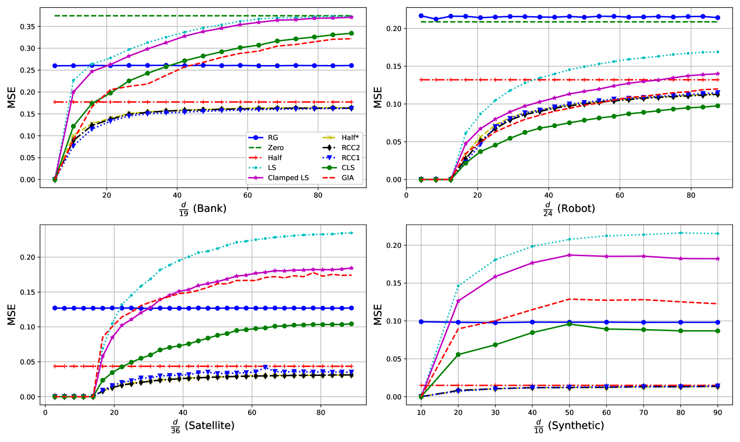
Figure 4: MSE per feature on Bank, Robot, Satellite and Synthetic datasets for different reconstruction attacks.

Figure 4 illustrates the performance of the aforementioned attacks versus the ratio of passive party’s features, i.e., $\frac{d}{d_{t}}$. The fact that when $d<k$, we have MSE$=0$ is due to the simple fact that the system of linear equations under consideration has a unique solution, i.e., $\mathbf{A}^{+}\mathbf{b}$. The first observation is provided as a remark

Remark 8.

It is observed that the scheme Half is always better than RG, which is consistent with theory (lemma 1), that states that any randomized guess is outperformed by its statistical mean. In Figure 4, the gap between the MSE corresponding to Half and RG is always $0.0833$, which is equal to $\textnormal{Var}(\hat{X})=\frac{1}{12}$ (with $\hat{X}$ being uniformly distributed on $[0,1]$) as expected from lemma 1. Therefore, as long as MSE is concerned, RG (used in [10, 11]) is not a proper baseline to choose. Moreover, it is observed that in the Bank, Satellite, and synthetic datasets, the simple scheme of Half outperforms LS (ESA) and GIA for the most part. The importance of this latter observation is more emphasized by noting that Half i) does not rely on any side information (either the receipt of confidence scores or the knowledge of passive party’s parameters.), and ii) does not need any optimization or matrix computation.

The second observation is the confirmation of Theorem 1, i.e., RCC2 performs better than Half^∗, which itself is better than Half. This rigorous guarantee that RCC2 and Half^∗ are always better than Half is crucial, since for the attacks CLS, LS (ESA) and GIA, there is no guarantee that they perform better than the trivial blind estimate of Half, which can be verified in Figure 4. The third observation is that Clamped LS performs better than LS (ESA), which is discussed before. The fourth observation is that the performance of RCC1 and RCC2 are close in these datasets, while no general claim can be made as to which is better than the other. The fifth observation is that either CLS or the simple Half^∗ outperform the results in the literature. We give the two final observations as remarks as follows.

Remark 9.

It is important to note that in general, the performance of the attack methods are data-dependent. In other words, one can synthesize a dataset, with an appropriate choice of the mean and variance, such that a particular attack exhibits promising performance. Nevertheless, in the context where the attacker is unaware of the underlying distribution of the passive party’s features, a reasonable method is that of estimation based on the Chebyshev center of the feasible solution space, and consequently, its approximations, i.e., RCC1 and RCC2. Although, there is no claim of universal optimality of the Chebyshev center (i.e., optimal for every dataset), it is in line with the intuition that in the worst possible case, it has the best performance, i.e., optimal in the best-worst sense.

Remark 10.

Consider a VFL model with two cases, where in the first one, features with the index set $[2]$ are given to the passive party and in the second case, passive party holds features indexed by $[4]$. Fix a specific attack method. It is obvious that MSE in the second case is greater than (or equal to) the MSE in the first case. But, how do the MSE per feature compare in these cases? This depends on the underlying distribution of the data. More specifically, the MSE per feature in the second case could be greater than, equal to, or even lower than that in the first case. This is because in MSE per feature, we have a ratio whose both numerator and denominator increase with the number of features; However, whether the overall ratio is increasing or decreasing depends on the rate of increase in the numerator which depends on the data. As an example, consider a binary classification VFL with $\hat{\mathbf{X}}_{\textnormal{LS}}$ as the attack method. First, assume that features indexed by $[2]$ are allocated to the passive party. In this case, the adversary has a non-zero MSE per feature, which is denoted by $\zeta$. Now, imagine that this time the passive party holds features indexed by $[d]$ for some $d>2$ to be obtained later. From (50), we have that the MSE per feature is upper bounded by $\frac{1}{d}\textnormal{Tr}(\mathbf{K}_{\mathbf{0}})$, where $\mathbf{K}_{\mathbf{0}}$ denotes the correlation matrix of the $d$ features. Assume that the distribution of the data is such that we have $\mathds{E}[X_{i}^{2}]=\frac{1}{i^{2}}$ for $i\in[d]$. As a result, we have that $\lim_{d\to\infty}\frac{1}{d}\textnormal{Tr}(\mathbf{K}_{\mathbf{0}})=0$, which means that we can select a $d>2$, such that the MSE per feature becomes smaller than $\zeta$, i.e., the case with $d=2$. Hence, in general, no claim can be made on the increasing/decreasing trend of the MSE per feature.

VIII-B Verification of Theorem 2

In Theorem 2 closed form expressions for the MSE of the attacks $\hat{\mathbf{X}}_{\textnormal{LS}}$ and $\hat{\mathbf{X}}_{\textnormal{half}^{*}}$ along with their corresponding upper and lower bounds are provided. Figure 5 provides the verification of this Theorem on four datasets. The empirical values, denoted by LS empirical and Half^∗ empirical, are the same curves as in the previous sebsection shown in Figure 4, i.e., by averaging over $N=1000$ predictions. The curves denoted by LS and Half^∗ denote the closed form expressions in (50) and (51), respectively, where the matrices $\mathbf{K}_{\mathbf{0}},\mathbf{K}_{\frac{1}{2}\mathbf{1}_{d}}$ and $\mathbf{K}_{\mathbf{\mu}}$ are empirically obtained over the whole datasets (including the training and test sets). First, we observe that LS and Half^∗ coincide with their corresponding empirical values. Moreover, we observe that the upper and lower bounds in (50) and (51), denoted by LS UB, Half^∗ UB, LS LB, and Half^∗ LB are valid. Note that the lower bound in (52) is denoted by LB. In particular, we observe that in the Bank dataset, the LS UB is tight when $d$ is large enough. Furthermore, it is observed that in the Satellite and synthetic datasets, the LB is tight for the attack Half^∗, which is justified by the fact that for these datasets, all the feature values are close to $\frac{1}{2}$ (see Figure 6) resulting in $\mathbf{K}_{\mathbf{\mu}}\approx\mathbf{K}_{\frac{1}{2}\mathbf{1}_{d}}$.

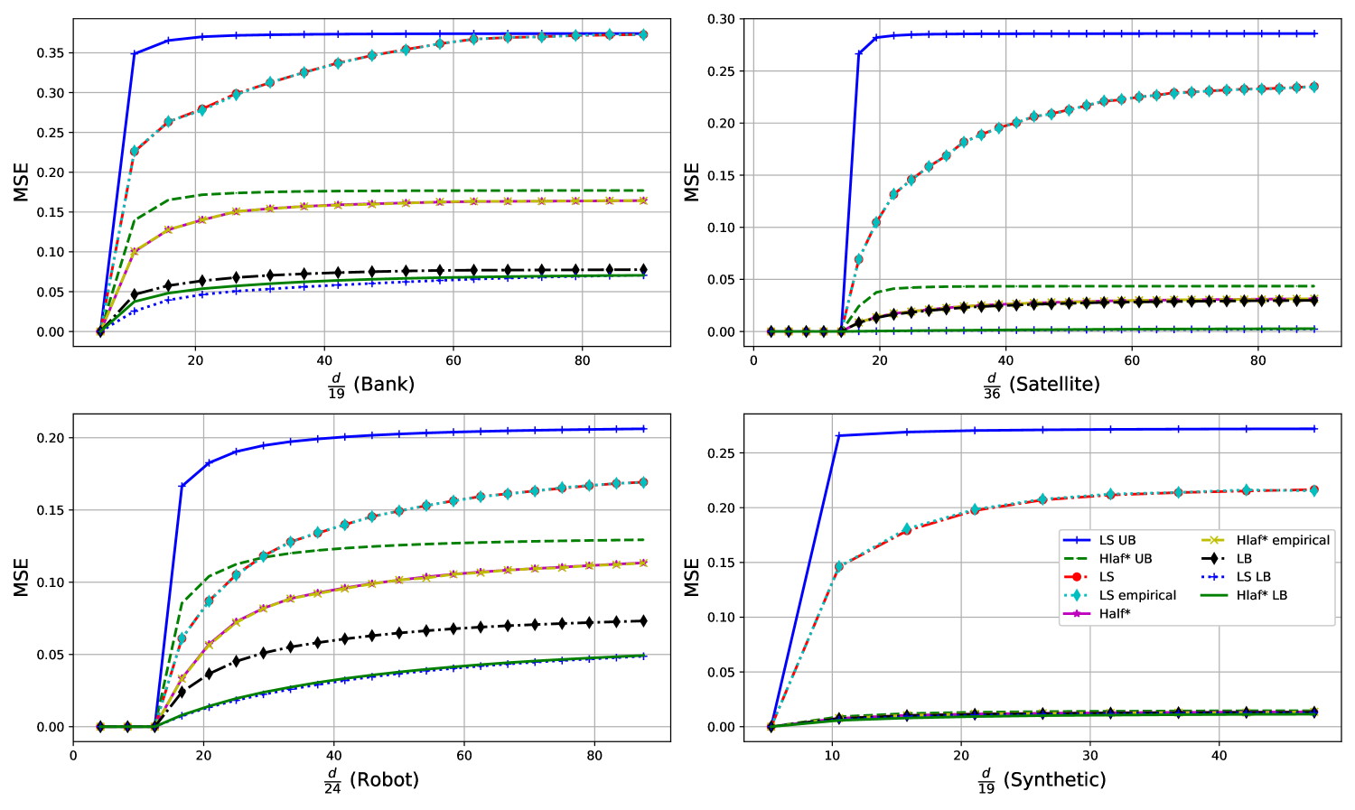
Figure 5: Illustration of the results of Theorem 2

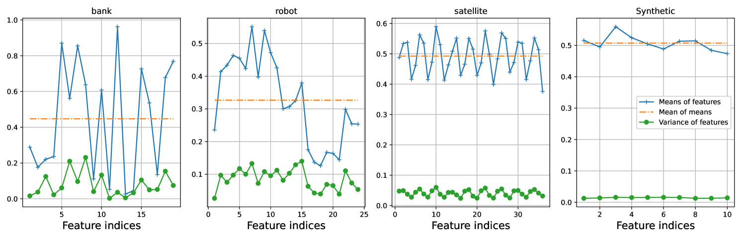
Figure 6: Empirical mean, variance, and mean of the means of features.

VIII-C Evaluation of the inference attack in the black-box setting

To evaluate the results in section VI, we assume that the 14th feature of the Bank data set, which denotes the employment variation rate in [20], is unknown. In other words, the passive party is allocated feature 14, and the active party has the remaining 18 features of this dataset. For this setting, the corresponding $\omega$ and $b$, given in section VI, are $\omega=0.98916,b=3.048751$, and as a result, we have $\omega b>0$. The adversary is unaware of the exact values of $\omega$ and $b$ and their signs. What it is informed of is only the fact that $\omega$ and $b$ have the same sign, and nothing else. According to the attack method in case 2 of section VI, the MSE converges in probability to 0 as the number of predictions $N$ grows. In Figure 7, the empirical expectation of $\frac{1}{N}\sum_{i=1}^{N}(X_{i}-\hat{X}_{i})^{2}$ is plotted for $N$ ranging from 1 to 100. For each $N$, the empirical expectation is obtained with averaging over 100 instances. As it can be verified in Figure 7, this expectation converges to 0, which by using Markov’s inequality, confirms that the empirical MSE converges in probability to 0.

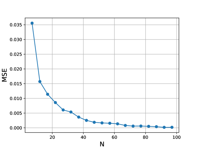
Figure 7: Inference attack in the black-box setting. The passive party holds one feature and $N$ denotes the number of predictions.

VIII-D Privacy-preserving scheme

In this section, the performance of the proposed privacy-preserving schemes in the two subsections of section VII is evaluated on real-world and synthetic data.

To evaluate the scheme in the first subsection, first, the LR is trained (with regularization) in the context of VFL without the privacy-preserving scheme and the performance of several attacks (LS, Clamped LS, CLS, Half^∗, RCC1 and RCC2) are obtained, as illustrated in Figures 8 to 11 with circle-blue lines.

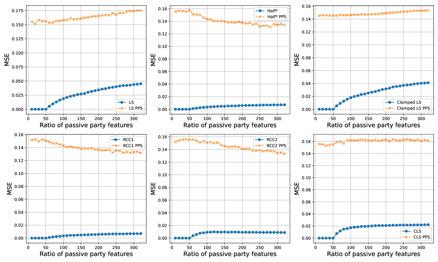
Figure 8: MSE per feature before and after applying PPS (Satellite).

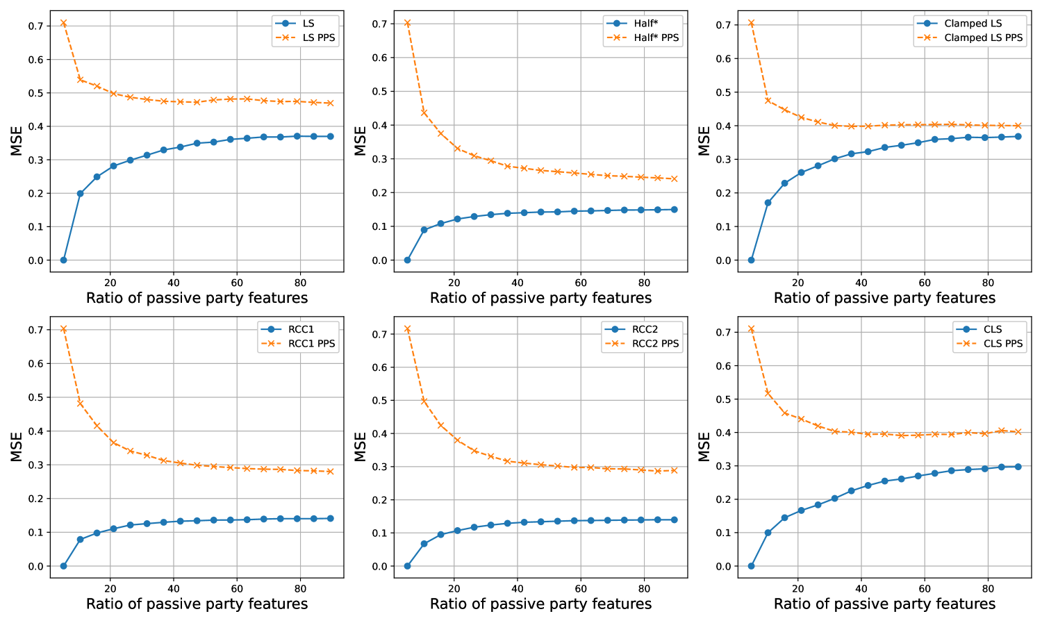
Figure 9: MSE per feature before and after applying PPS (Bank).

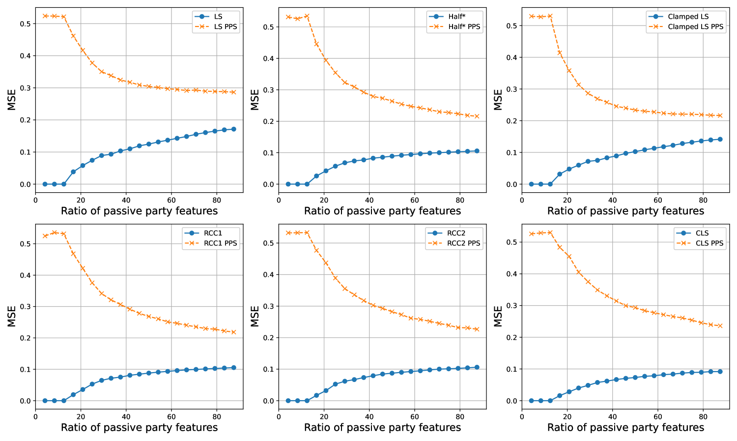
Figure 10: MSE per feature before and after applying PPS (Robot).

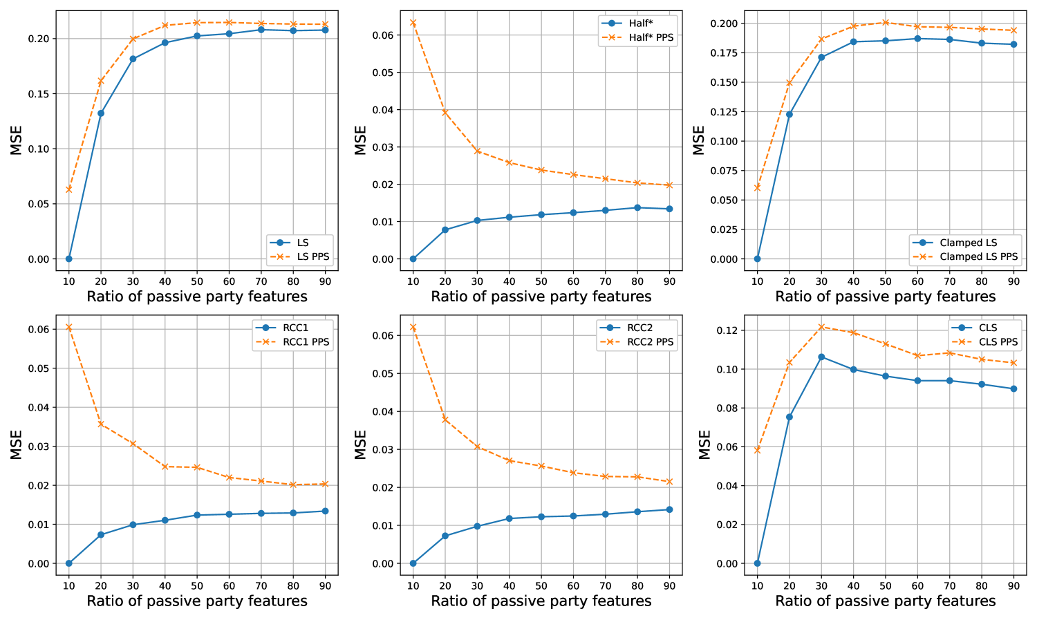
Figure 11: MSE per feature before and after applying PPS (Synthetic).

Next, we apply the PPS technique on the datasets to obtain new training sets, which are used to train new LR models. After the model is trained, the same reconstruction attacks are applied and their performance are evaluated by the MSE per feature shown in Figures 8 to 11 with dashed orange lines. As it can be observed, all the reconstruction attacks have become less successful in their estimation. It is important to note that multiplying the data by $-\mathbf{I}$ and then normalizing it is equivalent to changing each feature value $x$ to $1-x$. In what follows, we consider the least square attack analytically. As given in (50), we have

$$\textnormal{MSE}(\hat{\mathbf{X}}_{\textnormal{LS}})=\frac{\textnormal{Tr}\left((\mathbf{I}-\mathbf{A}^{+}\mathbf{A})\mathbf{K}_{\mathbf{0}}\right)}{d}.$$

Let $\textnormal{MSE}(\hat{X}_{\textnormal{LS}}^{\textnormal{PPS}})$ denote the MSE per feature of this attack after PPS has been applied. Since we have $\mathbf{W}=\mathbf{W}_{0}\mathbf{H}^{-1}=-\mathbf{W_{0}}$, we conclude that the new matrix $\mathbf{A}$ that the adversary constructs when PPS has been applied is the negative of that in the case without PPS. As a result, we have

$$\textnormal{MSE}(\hat{X}_{\textnormal{LS}}^{\textnormal{PPS}})=\frac{1}{d}\mathds{[}\|\mathbf{X}-\mathbf{A}^{+}\mathbf{A}(\mathbf{1}-\mathbf{X})\|^{2}].$$

By simple calculations, we get

$$\textnormal{MSE}(\hat{X}_{\textnormal{LS}}^{\textnormal{PPS}})-\textnormal{MSE}(\hat{\mathbf{X}}_{\textnormal{LS}})=\frac{4}{d}\textnormal{Tr}(\mathbf{A}^{+}\mathbf{A}\mathbf{K}_{\frac{1}{2}\mathbf{1}})\geq 0.$$

The closer the features are to $\frac{1}{2}$, the lower $\textnormal{Tr}(\mathbf{K}_{\frac{1}{2}\mathbf{1}})$ is, and the above difference is smaller. This is consistent with the intuition since in this case $x$ and $1-x$ are not far from each other. Interestingly, we can obtain the similar performance degradation for $\textnormal{MSE}(\hat{X}_{\textnormal{half}^{*}}^{\textnormal{PPS}})$ as

$$\textnormal{MSE}(\hat{X}_{\textnormal{half}^{*}}^{\textnormal{PPS}})-\textnormal{MSE}(\hat{\mathbf{X}}_{\textnormal{half}^{*}})=\frac{4}{d}\textnormal{Tr}(\mathbf{A}^{+}\mathbf{A}\mathbf{K}_{\frac{1}{2}\mathbf{1}}).$$

As we know, $\mathbf{A}^{+}\mathbf{A}$ has $\textnormal{rank}(\mathbf{A})$ 1’s and $\textnormal{nul}(\mathbf{A})$ 0’s as eigenvalues. In the experimental results, the rank of $\mathbf{A}$ is $\min\{k-1,d\}$. Therefore, denoting the eigenvalues of $\mathbf{K}_{\frac{1}{2}\mathbf{1}}$ by $\gamma_{1}\geq\gamma_{2}\geq\ldots\geq\gamma_{d}$, by applying Von Neumann’s trace inequality, we have

$$\frac{4}{d}\textnormal{Tr}(\mathbf{A}^{+}\mathbf{A}\mathbf{K}_{\frac{1}{2}\mathbf{1}})\leq\frac{4}{d}\sum_{i=1}^{\min\{k-1,d\}}\gamma_{i}.$$

If the data is such that the maximum eigenvalue, i.e., $\gamma_{1}$, scales at most sublinearly with $d$ ($\lim_{d\to\infty}\frac{\gamma_{1}}{d}=0$), it can be concluded that for a fixed number of classes $k$, the difference vanishes as $d$ grows.

To show that this PPS does not alter the confidence scores, the average KL divergence between confidence scores obtained before and after the application of PPS, averaged over $N^{\prime}=20000$ samples, is illustrated in Figure 12. In other words, if the confidence scores of sample $i$ before and after the application of PPS are denoted by $\mathbf{c}_{i}$ and $\tilde{\mathbf{c}}_{i}$, respectively, the average KL divergence is $\frac{1}{N^{\prime}}\sum_{i=1}^{N^{\prime}}D(\mathbf{c}_{i}||\tilde{\mathbf{c}}_{i})$. This value, as shown in Figure 12, is close to 0, which is consistent with our notion of a lossless PPS. The slight deviation from 0 is due to i) normalization of features, and ii) the step size of the gradient optimizer.

Finally, it is important to note that if the adversary is aware of $\mathbf{H}$, the privacy-preserving scheme fails. If the adversary is unaware of this transformation, still he/she could perform the attack assuming that in half of the samples, the features haven’t been transformed and in the remaining ones, they have. Still, with a similar argument as in the black-box setting, it can be shown that this assumption cannot beat the scheme $\hat{\mathbf{X}}_{\textnormal{half}}$. There are other variants of this transform, e.g., selectively transform some features and preserve the remaining ones. Permutation can also be applied in case the features have similar alphabets, etc.

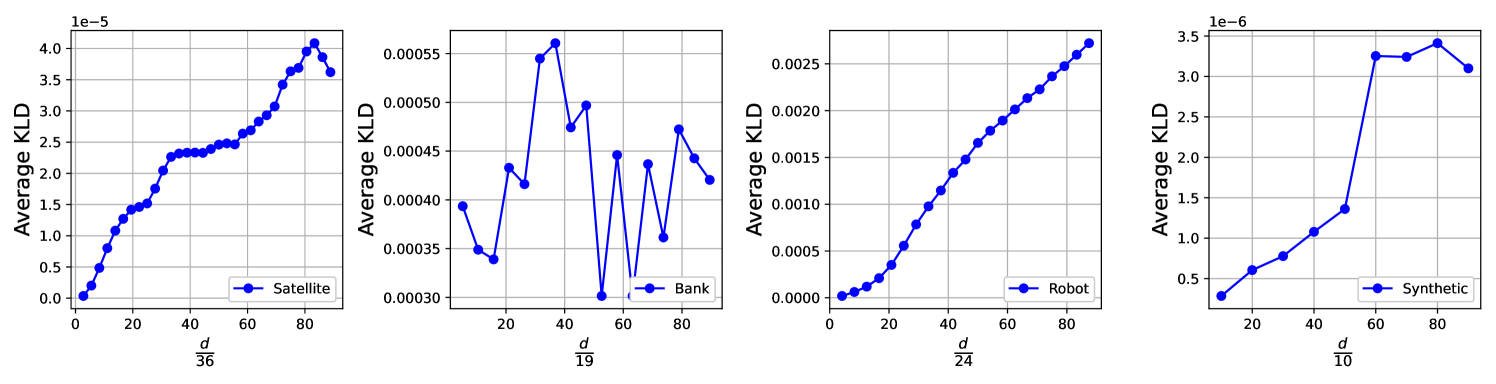
Figure 12: Average KL divergence between the confidence scores before and after the application of PPS.

To evaluate the schemes in the second subsection of section VII, Figure 13 illustrates the privacy-preserving schemes (Schemes 1 and 2) in red and dark blue curves. The vertical axis refers to the MSE per feature for $\hat{\mathbf{X}}_{\textnormal{half}^{*}}$ and the horizontal axis denotes the average KL distance between the confidence scores before and after the application of these schemes. Furthermore, two other curves (denoted by ”scheme 3” and ”class label”) are also plotted which are explained as follows. Scheme 3, shown in green, refers to the scheme in which $\tilde{\mathbf{z}}\triangleq(1-\alpha)\mathbf{z}+\alpha\mathbf{1}$ for $\alpha\in[0,1)$. Obviously, this scheme preserves the model accuracy, and by tuning $\alpha$, the trade-off in Figure 13 is obtained. The curve denoted by ”class label” represents the scenario where the coordinator reveals the class label. In doing so, the confidence score which is maximum is mapped to 1, and the remaining ones are mapped to 0. However, in order to obtain the trade-off in Figure 13, we let these remaining confidence scores approach 0. The smaller they get, the greater the average KL distance becomes, and in this way, the pale blue curve is produced.

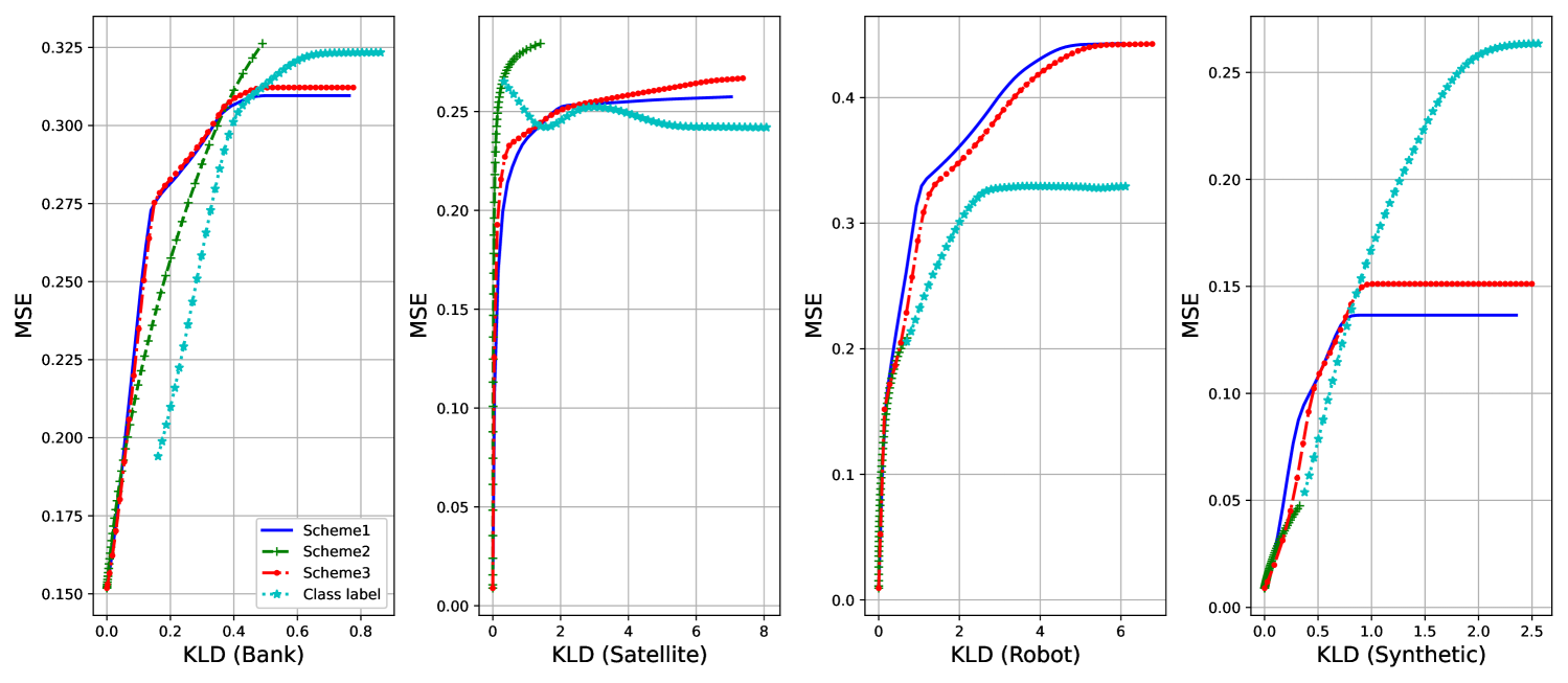
Figure 13: Privacy-preserving schemes that preserve the model accuracy

VIII-E A note on the effect of the initial point in GIA

As part of the experimental results, simulation of GIA was required for comparison purposes. In doing so, [11, Algorithm 1] was considered, in which the initial point of the gradient-based method is set to the origin, i.e., $\mathbf{0}_{d}$. Knowing that the gradient-based methods start with the initial point and move in the direction opposite to the gradient of the objective function, this choice of the initial point makes sense when the features are relatively close to zero. However, when the adversary has no information about the distribution of the passive party’s features, a better approach in the best-worst sense, is to take $\frac{1}{2}\mathbf{1}_{d}$, i.e., the Chebyshev center of $[0,1]^{d}$, as the initial point. This observation is shown in Figure 14, where the performance of GIA is illustrated for different initializations, namely, $\mathbf{0}_{d}$ (original in [11]), $\frac{1}{2}\mathbf{1}_{d}$ and random (uniform over $[0,1]^{d}$). We observe that in the Bank, Sattelite and synthetic datasets whose features have a mean close to $\frac{1}{2}$ (see Figure 6), initialization with $\frac{1}{2}\mathbf{1}_{d}$ is the best, while in the Robot dataset whose features are relatively far from $\frac{1}{2}\mathbf{1}_{d}$, initialization with $\frac{1}{2}\mathbf{1}_{d}$ still performs better for the most part. Therefore, although in the context of this paper, GIA is outperformed by the proposed attack methods, it makes sense to use the initialization $\frac{1}{2}\mathbf{1}_{d}$ when the adversary is blind to the underlying distribution of the passive party’s features.

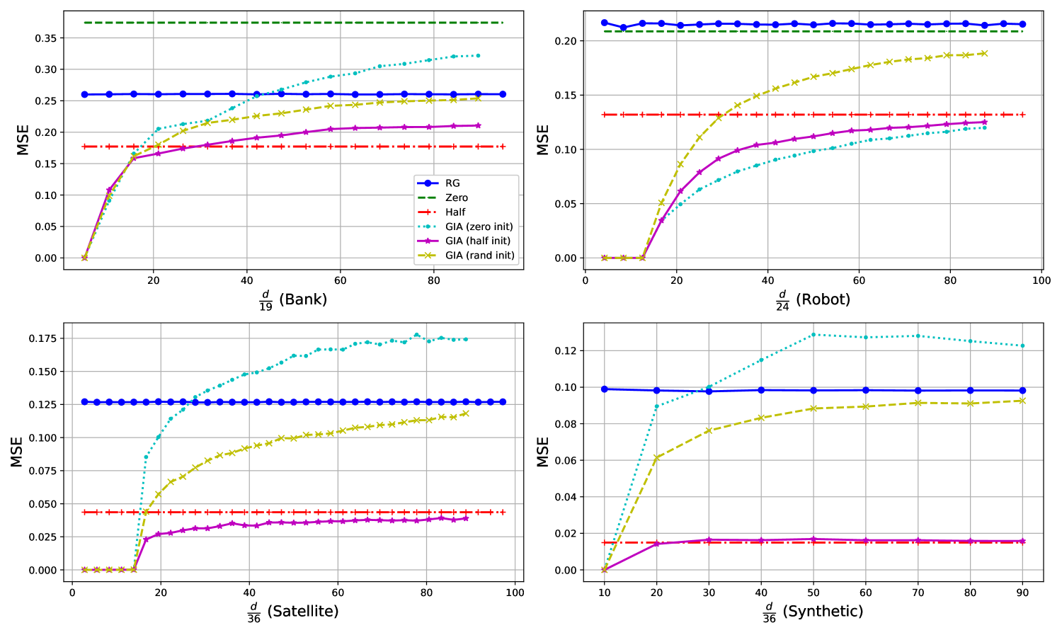
Figure 14: MSE per feature in GIA for different initialization.

IX conclusions

In this paper, a vertical federated learning setting is considered, where an active party, having access to true class labels, wishes to build a classification model by utilizing more features from a passive party, that has no access to the labels, to improve the model accuracy. The model under consideration is logistic regression. In the prediction phase, based on a classical notion of the centre of the set of feasible solutions, several inference attack methods are proposed that the active party can apply to reconstruct the sensitive information of the passive party. These attacks are shown to outperform those proposed in the literature. Moreover, several theoretical performance guarantees, in terms of upper and lower bounds, are provided for the aforementioned attacks. Subsequently, we show that in the black-box setting, knowing only the signs of the parameters involved is sufficient for the adversary to fully reconstruct the passive party’s features in certain scenarios. As a defense mechanism, two privacy-preserving schemes are proposed that worsen the adversary’s reconstruction attacks, while preserving the confidence scores revealed to the active party. Finally, experimental results demonstrate the effectiveness of the proposed attacks and the privacy-preserving schemes.

Two complementary points are worth mentioning here. The first one is that in the proposed inference attacks, no knowledge about the nature of the features was used. In other words, all the features were regarded as real numbers in the interval $[0,1]$. However, in practice, features can have sparse values. For example, if a feature denotes the marital status, it has two values, and after normalizing to the range $[0,1]$, it takes either 0 or 1. Now, assume as an example that the equation under consideration is $x_{1}+x_{2}=0.5$. This equation has infinite solutions in $[0,1]^{2}$, while it has only one solution in $[0:1]\times[0,1]$, which is $(0,0.5)$. Hence, all the attack methods can further be improved by utilizing this knowledge of the adversary.

We proceed with this example to mention the second point, which is the limitation of the mean square error (MSE) as a performance metric. Assume that the passive party holds features corresponding to ”marital status” and ”salary”, and the adversary is aware of this, though it doesn’t know the ordering, i.e., whether $x_{1}$ denotes the salary or $x_{2}$. Assume that in this context $x_{1}$ and $x_{2}$ denote ”marital status” and ”salary”, respectively. Consider $N$ prediction records with true values $\mathbf{X}_{1}=(0,0.18)^{T},\mathbf{X}_{2}=(1,0.66)^{T},\mathbf{X}_{3}=(0,0.44)^{T},\ldots,\mathbf{X}_{N}=(1,0.77)^{T}$. Assume that what the adversary reconstructs is a permuted version of the true values, i.e., $\hat{\mathbf{X}}_{1}=(0.18,0)^{T},\hat{\mathbf{X}}_{2}=(0.66,1)^{T},\hat{\mathbf{X}}_{3}=(0.44,0)^{T},\ldots,\hat{\mathbf{X}}_{N}=(0.77,1)^{T}$. It is obvious that MSE$\neq 0$, meaning that the adversary cannot perfectly reconstruct the features. However, knowing the set of features that have been estimated, upon observing the estimates, an intelligent adversary decides that the second element in each estimate refers to marital status, as it takes only 0 and 1, and the first element in each estimate refers to salary. Therefore, although MSE of this reconstruction is not zero, the adversary is able to perfectly reconstruct the features. This shows the limitation of the popular MSE metric by which the attacks are evaluated, and hence, needs further investigation, esp. when the support of the features are disparate/distinguishable. For instance, assuming that the alphabets of features are finite, which is the case in many practical scenarios, the conditional entropy of the true values conditioned on the reconstructions better captures the adversary’s performance in this context, i.e., here, we have $H(\mathbf{X}|\hat{\mathbf{X}})=0$.

References

- [1] B. McMahan, E. Moore, D. Ramage, S. Hampson, and B. A. y. Arcas, “Communication-Efficient Learning of Deep Networks from Decentralized Data,” in Proceedings of the 20th International Conference on Artificial Intelligence and Statistics, ser. Proceedings of Machine Learning Research, A. Singh and J. Zhu, Eds., vol. 54. PMLR, 20–22 Apr 2017, pp. 1273–1282. [Online]. Available: https://proceedings.mlr.press/v54/mcmahan17a.html
- [2] S. Lu, Y. Zhang, and Y. Wang, “Decentralized federated learning for electronic health records,” in 2020 54th Annual Conference on Information Sciences and Systems (CISS), 2020, pp. 1–5.
- [3] W. Li, F. Milletari, D. Xu, N. Rieke, J. Hancox, W. Zhu, M. Baust, Y. Cheng, S. Ourselin, M. J. Cardoso, and A. Feng, “Privacy-preserving federated brain tumour segmentation,” CoRR, vol. abs/1910.00962, 2019. [Online]. Available: http://arxiv.org/abs/1910.00962
- [4] F. Beaufays, K. Rao, R. Mathews, and S. Ramaswamy, “Federated learning for emoji prediction in a mobile keyboard,” 2019. [Online]. Available: https://arxiv.org/abs/1906.04329
- [5] A. Hard, K. Rao, R. Mathews, F. Beaufays, S. Augenstein, H. Eichner, C. Kiddon, and D. Ramage, “Federated learning for mobile keyboard prediction,” CoRR, vol. abs/1811.03604, 2018. [Online]. Available: http://arxiv.org/abs/1811.03604
- [6] K. Yang, T. Fan, T. Chen, Y. Shi, and Q. Yang, “A quasi-newton method based vertical federated learning framework for logistic regression,” CoRR, vol. abs/1912.00513, 2019. [Online]. Available: http://arxiv.org/abs/1912.00513
- [7] Y. Wang, Y. Tian, X. Yin, and X. Hei, “A trusted recommendation scheme for privacy protection based on federated learning,” CCF Transactions on Networking, vol. 3, pp. 218–228, 12 2020.
- [8] R. Yu and P. Li, “Toward resource-efficient federated learning in mobile edge computing,” IEEE Network, vol. 35, no. 1, pp. 148–155, 2021.
- [9] Y. Cheng, Y. Liu, T. Chen, and Q. Yang, “Federated learning for privacy-preserving ai,” Commun. ACM, vol. 63, no. 12, p. 33–36, nov 2020. [Online]. Available: https://doi.org/10.1145/3387107
- [10] X. Luo, Y. Wu, X. Xiao, and B. C. Ooi, “Feature inference attack on model predictions in vertical federated learning,” CoRR, vol. abs/2010.10152, 2020. [Online]. Available: https://arxiv.org/abs/2010.10152
- [11] X. Jiang, X. Zhou, and J. Grossklags, “Comprehensive analysis of privacy leakage in vertical federated learning during prediction,” Proceedings on Privacy Enhancing Technologies, vol. 2022, pp. 263–281, 04 2022.
- [12] A. C. Yao, “Protocols for secure computations,” in 23rd Annual Symposium on Foundations of Computer Science (sfcs 1982), 1982, pp. 160–164.
- [13] I. Damgård and M. Jurik, “A generalisation, a simplification and some applications of paillier’s probabilistic public-key system,” in Public Key Cryptography, K. Kim, Ed. Berlin, Heidelberg: Springer Berlin Heidelberg, 2001, pp. 119–136.
- [14] R. Penrose, “A generalized inverse for matrices,” Mathematical Proceedings of the Cambridge Philosophical Society, vol. 51, no. 3, p. 406–413, 1955.
- [15] T. Narang, “On Chebyshev centers in metric spaces,” Publications de l’Institut Mathematique, vol. 106, no. 120, pp. 47–51, 2019.
- [16] E. Welzl, “Smallest enclosing disks (balls and ellipsoids),” in New Results and New Trends in Computer Science, H. Maurer, Ed. Berlin, Heidelberg: Springer Berlin Heidelberg, 1991, pp. 359–370.
- [17] N. D. Botkin and V. L. Turova-Botkina, “An algorithm for finding the chebyshev center of a convex polyhedron,” Applied Mathematics and Optimization, vol. 29, pp. 211–222, 1993.
- [18] Y. C. Eldar, A. Beck, and M. Teboulle, “A minimax Chebyshev estimator for bounded error estimation,” IEEE Transactions on Signal Processing, vol. 56, no. 4, pp. 1388–1397, 2008.
- [19] A. W. Marshall, I. Olkin, and B. C. Arnold, Inequalities: Theory of Majorization and its Applications, 2nd ed. Springer, 2011, vol. 143.
- [20] D. Dua and C. Graff, “UCI machine learning repository,” 2017. [Online]. Available: http://archive.ics.uci.edu/ml
- [21] A. W. Lo and A. C. MacKinlay, “Data-Snooping Biases in Tests of Financial Asset Pricing Models,” The Review of Financial Studies, vol. 3, no. 3, pp. 431–467, 04 2015. [Online]. Available: https://doi.org/10.1093/rfs/3.3.431
- [22] github, “Github,” 2020. [Online]. Available: https://github.com/mrtzvrst
- [23] S. Diamond and S. Boyd, “CVXPY: A Python-embedded modeling language for convex optimization,” Journal of Machine Learning Research, vol. 17, no. 83, pp. 1–5, 2016.