Revisiting the central limit theorems for the SGD-type methods

Abstract

We revisited the central limit theorem (CLT) for stochastic gradient descent (SGD) type methods, including the vanilla SGD, momentum SGD and Nesterov accelerated SGD methods with constant or vanishing damping parameters. By taking advantage of Lyapunov function technique and $L^{p}$ bound estimates, we established the CLT under more general conditions on learning rates for broader classes of SGD methods compared with previous results. The CLT for the time average was also investigated, and we found that it held in the linear case, while it was not generally true in nonlinear situation. Numerical tests were also carried out to verify our theoretical analysis.

Keywords Central limit theorem, SGD, momentum SGD, Nesterov acceleration

1 Introduction

We consider the problem

$$\begin{split}\min_{x\in\mathbb{R}^{d}}f(x):=\frac{1}{S}\sum_{i=1}^{S}f_{i}(x),\end{split}$$ (1)

where $f,f_{i}:\mathbb{R}^{d}\rightarrow\mathbb{R}$ are continuously differentiable functions. When $S$, usually the number of samples in machine learning, is very large, one can utilize the well-known stochastic gradient descent (SGD) iteration

$$\begin{split}x_{k}&=x_{k-1}-\alpha_{k}\nabla f_{s_{k}}(x_{k-1})\\ &=x_{k-1}-\alpha_{k}\nabla f(x_{k-1})+\alpha_{k}\xi_{k}\end{split}$$ (2)

to approximately locate the minima of $f$ under suitable convexity condition, where $\alpha_{k}$ is the learning rate, $s_{k}$ is a random variable uniformly sampled from $\{1,2,\ldots,S\}$. In (2), the noise term $\xi_{k}=\nabla f(x_{k-1})-\nabla_{s_{k}}f(x_{k-1})$ satisfies the centering condition $\mathbb{E}[\xi_{k}|x_{k-1}]=0$.

There has been a lot of extensions and theoretical analysis on SGD-type methods in the literature. To be precise, we denote a vanilla SGD (vSGD) with a general Markovian iteration form

$$x_{k}=x_{k-1}-\alpha_{k}F(x_{k-1},\xi_{k}),$$ (3)

where $\mathbb{E}[F(x_{k-1},\xi_{k})|x_{k-1}]=\nabla f(x_{k-1})$. Its different variants, such as the momentum SGD (mSGD) (SGD version of Polyak’s Heavy-ball method [17])

$$\begin{split}v_{k}&=\beta_{k}v_{k-1}-\alpha_{k}F(x_{k-1},\xi_{k}),\\ x_{k}&=x_{k-1}+v_{k},\end{split}$$ (4)

or the Nesterov accelerated form (NaSGD) [14]

$$\begin{split}x_{k}&=y_{k-1}-\alpha_{k}F(y_{k-1},\xi_{k}),\\ y_{k}&=x_{k}+\beta_{k}(x_{k}-x_{k-1}),\end{split}$$ (5)

are also widely used to speed up the convergence, where $\beta_{k}\in[0,1)$ in both expressions. For vSGD (3), a well-known result is that the almost sure convergence of $\{x_{k}\}$ towards a critical point of $f$ holds when the learning rates $\{\alpha_{k}\}$ fulfill the typical condition $\sum\alpha_{k}=\infty$ and $\sum\alpha_{k}^{2}<\infty$ even for nonconvex problems [3]. The first non-asymptotic convergence rate was obtained in [7] with the form $\min_{k\leq n}\mathbb{E}\|\nabla f(x_{k})\|^{2}=O(1/\sqrt{n})$, which is un-improvable in general even when $f$ is (non-strongly) convex. This rate can be improved to be $O(1/n)$ when the variance reduction technique was utilized [19]. However, for strongly convex $f$, the optimal convergence rate can be shown to be $\mathbb{E}\|\nabla f(x_{n})\|^{2}=O(1/n)$ (or similar estimates with respect to $f(x_{n})-f(x^{*})$ or $\|x_{k}-x^{*}\|^{2}$, where $x^{*}$ is the unique minima) when the learning rate $\alpha_{k}=O(1/k)$ [5, 13, 16]. By contrast, the analysis for the mSGD and NaSGD are relatively few. The asymptotic convergence of a general class of SGD with momentum was proven in [2], and the convergence rate of the time averaged $\mathbb{E}\|\nabla f(x_{k})\|^{2}$ of mSGD was studied in [9]. The stationary convergence bound of this time averaging was also established in [12] when the learning rates are constant. For Nesterov acceleration gradient, it is well-known that the convergence rate of $f(x_{n})$ towards $f(x^{*})$ is $O(n^{-2})$ in deterministic case when $f$ is convex [22]. And the stationary convergence bound of NaSGD was studied in [1] when the learning rates are constant.

Besides the aforementioned convergence analysis, it is a natural question to study the law of fluctuations after knowing the convergence of $\{x_{k}\}$, which is expected to be related to the central limit theorem (CLT) in classical probability theory. However, this topic is less well studied in the literature. We would like to mention that the CLT was investigated in [6] for the SGD-type methods with/without momentum. And it was obtained that the convergence in distribution

$$\begin{split}\frac{x_{n}-x^{*}}{\sqrt{\alpha_{n}}}\Rightarrow N(0,V)\end{split}$$ (6)

under the condition that $f$ is strongly convex and $\sum_{k=1}^{\infty}\alpha_{k}^{3/2}<+\infty$, where $V$ is the asymptotic covariance matrix. In [4], the condition had relaxed to $\sum_{k=1}^{\infty}\alpha_{k}^{2}<+\infty$. The CLT for the variance reduced SGD (SVRG) can be enhanced to $(x_{n}-x^{*})/a^{n}\Rightarrow N(0,V)$ for some $a\in(0,1)$ [11]. It was also shown that $(\hat{x}_{n}-x^{*})/\sqrt{n}\Rightarrow N(0,V)$ where $\hat{x}_{n}:=\sum_{k=1}^{n}x_{k}/n$ is the empirical average of $x_{k}$ [18]. And a continuous time version of CLT was given in [21] when $f$ is strongly convex.

The purpose of this paper is to give a systematic restudy on the CLT for the SGD-type methods. We will consider the CLT for the vSGD (3), NaSGD (5), and the mSGD with the form

$$\begin{split}v_{k}&=(1-\beta_{k})v_{k-1}-\alpha_{k}F(x_{k-1},\xi_{k}),\\ x_{k}&=x_{k-1}+\alpha_{k}v_{k},\end{split}$$ (7)

where $\beta_{k}=\mu_{k}\alpha_{k}$ and $\mu_{k}>0$ is a damping parameter. We take the form (7) instead of (4) due to its better connection with the continuous time limit.

The main contributions of this paper are in three folds.

1. CLT for vSGD. We re-establish the CLT for vSGD by borrowing the idea in [21]. But our different setup on the assumptions on noise and learning rates complicates the overall analysis, which is different from that taken in [6] and [21]. With our approach, we can get the same CLT form (6) as in [6] but only require the learning rates satisfy the condition (10) and the so-called slow condition (see Assumption (A2)). This relieves the conditions on $\{\alpha_{k}\}$ in [6], which requires $\sum_{k}\alpha_{k}^{2}<\infty$ in linear case and $\sum_{k}\alpha_{k}^{3/2}<\infty$ in nonlinear case (i.e., $\nabla f(x)$ is linear or nonlinear on $x$).

2. CLT for mSGD and NaSGD. This part can be classified into two cases: the case with constant damping $\mu_{k}\equiv\tilde{\mu}$, or the case with vanishing damping $\mu_{k}\rightarrow 0$. In the continuum limit, this corresponds to the SDEs

   $$\ddot{x}+\mu(t)\dot{x}+\nabla f(x)+\xi=0$$ (8)

   with constant or vanishing damping $\mu(t)$ [22]. Taking advantage of the Lyapunov function technique, we can show the CLT holds for both cases. The CLT for the vanishing damping case has never been studied before, and the constant damping case was only implicitly considered for the mSGD in the linear case in [6], but with stronger requirement $\sum_{k}\alpha_{k}^{2}<\infty$. Besides, a two-time-scale stochastic approximation was given in [4],

   $$\begin{split}w_{k}&=w_{k-1}-\alpha_{k}(A_{11}w_{k-1}+A_{12}u_{k-1}+\xi_{k}),\\ u_{k}&=u_{k-1}-\beta_{k}(A_{21}w_{k-1}+A_{22}u_{k-1}+\eta_{k}),\end{split}$$

   where $\alpha_{k}=o(\beta_{k})$, which is quite different from the mSGD shown in Section 4.

3. CLT for the time average of $x_{k}$. We discussed the CLT for the time average:

   $$\bar{x}_{n}=\frac{\sum_{k=1}^{n}\alpha_{k}x_{k-1}}{\sum_{k=1}^{n}\alpha_{k}},$$ (9)

   which is the discrete analog of the continuous time average $\int_{0}^{T}x(t)dt/T$, where $T$ is the summation of step size. Interestingly, we found that the CLT of the form $T_{n}/\sqrt{S_{n}}\cdot(\bar{x}_{n}-x^{*})\Rightarrow N(0,V)$ holds in the linear case, while it is not true in general nonlinear case (see details in Sec. 5).

The rest of this paper is organized as follows. We will prove the CLT for the vSGD, mSGD and NaSGD, and the time average $\bar{x}_{n}$ in Sections 3, 4 and 5, respectively. Then we present numerical examples to verify the obtained CLT results in Section 6. Finally, we make the conclusion. Some proof details are left in the Appendix.

2 Assumptions and Lemmas

Let us first present some preliminary mathematical setup utilized in this paper. We will always assume the following necessary condition on $\{\alpha_{k}\}$ to ensure the convergence of $\{x_{k}\}$ to $x^{*}$ when $f$ is strongly convex.

Assumption A.

Assumptions on the learning rates.

1. ($\mathbf{Divergence~{}condition}$) The learning rates $\{\alpha_{k}\}$ satisfy

   $$\lim_{k\rightarrow\infty}\alpha_{k}=0,\quad\sum_{k=1}^{\infty}\alpha_{k}=\infty.$$ (10)

2. ($h_{0}$-$\mathbf{slow~{}condition})$ The learning rates $\{\alpha_{k}\}$ are said to satisfy the $h_{0}$-slow condition with $h_{0}>0$ if $\{\alpha_{k}\}$ fulfill Assumption (A1) and

   $$\exists K_{s}>0,\text{ such that }\quad\frac{\alpha_{n}}{\alpha_{m}}\geq K_{s}\prod_{k=m+1}^{n}(1-h_{0}\alpha_{k})\quad\text{ for any }\ n>m\text{ large enough}.$$ (11)

3. ($\mathbf{Sufficient~{}decrease~{}condition}$) The learning rates $\{\alpha_{k}\}$ are said to be sufficiently decreasing if $\{\alpha_{k}\}$ fulfill Assumption (A1) and

   $$\exists d_{0}\geq 0,\text{ such that }\quad\frac{\alpha_{k}-\alpha_{k+1}}{\alpha_{k}}=d_{0}\alpha_{k}+o(\alpha_{k})\quad\text{for large enough }k.$$ (12)

   Indeed we have $d_{0}=\lim_{k\rightarrow\infty}(\alpha_{k}-\alpha_{k+1})/\alpha_{k}^{2}\geq 0$ if $\{\alpha_{k}\}$ satisfy sufficient decrease condition.

Note that if $\{\alpha_{k}\}$ satisfy the $h_{0}$-slow condition, then they also satisfy $h$-slow condition for any $h>h_{0}$. The proposed $h_{0}$-slow condition is weak enough to cover some commonly used learning schedules with slower decreasing rate than $O(1/k)$, while strong enough to build up our CLT estimates.

It is straightforward to observe that if $\{\alpha_{k}\}$ are sufficiently decreasing, they will fulfill the $h_{0}$-slow condition for any $h_{0}>d_{0}$ since

$$\frac{\alpha_{n}}{\alpha_{m}}=\prod_{k=m}^{n-1}\left(1-d_{0}\alpha_{k}-o(\alpha_{k})\right)\geq\frac{1}{2}\prod_{k=m+1}^{n}(1-h_{0}\alpha_{k})\quad\text{for large enough }m.$$

Typical examples which satisfy $h_{0}$-slow condition and sufficient decrease condition include:

1. $\alpha_{k}=K/k^{a},K>0,a\in(0,1)$, then $d_{0}=0$.

2. $\alpha_{k}=K/k,K>0$, then $d_{0}=K^{-1}$.

3. $\beta_{k}=k\alpha_{k}$ increases to infinity monotonically, e.g. $\alpha_{k}=Ck^{-a}\ln k,a\in(0,1]$, then

   $$d_{0}=\lim_{k\rightarrow\infty}\alpha_{k}^{-1}\left(1-\frac{k\beta_{k+1}}{(k+1)\beta_{k}}\right)\leq\lim_{k\rightarrow\infty}\frac{1}{(k+1)\alpha_{k}}=0.$$

4. If $\{\alpha_{k}\}$ satisfy the $h_{0}$-slow condition and $\{\eta_{k}\}$ is a bounded positive sequence, i.e., $0<\inf_{k}{\eta_{k}}\leq\sup_{k}{\eta_{k}}<+\infty$, then $\{\alpha_{k}\eta_{k}\}$ satisfy the $h_{0}/\inf_{k}{\eta_{k}}$-slow condition.

Define the filtration

$$\mathcal{F}_{k}=\sigma(x_{0},\xi_{1},\xi_{2},\cdots,\xi_{k}),$$ (13)

i.e., the $\sigma$-algebra generated by $(x_{0},\xi_{1},\ldots,\xi_{k})$. Denote by $X_{n}\overset{p}{\rightarrow}X$ the convergence in probability, i.e., $\lim_{n\rightarrow\infty}\mathbb{P}(\|X_{n}-X\|\geq\varepsilon)=0$ for any $\varepsilon>0$, where $\|\cdot\|$ could be any norm for $X_{n},X\in\mathbb{R}^{d}$ or $\mathbb{R}^{d\times d}$ because of the norm equivalence theorem in finite dimensions.

Assumption B.

Statistics for $\{\xi_{k}\}$ and initial value.

1. We assume the following conditional mean and covariance conditions for the noise term $\{\xi_{k}\}$ in SGD-type methods

   $$\mathbb{E}[\xi_{k}|\mathcal{F}_{k-1}]=0,\quad\mathbb{E}[\xi_{k}\xi_{k}^{T}|\mathcal{F}_{k-1}]\overset{p}{\rightarrow}\Sigma\succ 0,$$ (14)

   where the notation ‘$A\succ B$’ means $A-B$ is a symmetric positive definite (SPD) matrix.

2. For the initial value $x_{0}$, we assume that there exists large enough $p\geq 2$, such that $\mathbb{E}\|x_{0}\|^{p}<\infty$ and $\mathbb{E}|f(x_{0})|<\infty$.

3. Assumption (A4), (A5) hold, and there exist $\delta_{0},M,K_{\xi}>0$ such that

   $$\mathbb{E}\big{[}\|\xi_{k}\|^{2+\delta_{0}}|\mathcal{F}_{k-1}\big{]}\leq M+K_{\xi}\|\nabla f(x_{k-1})\|^{2+\delta_{0}}.$$ (15)

Remark 2.1.

Assumption (A4) on $\left\{\xi_{k}\right\}$ holds naturally for the incremental SGD form (2) in practice. According to [3], one can establish the convergence of SGD by supplementing the condition like $\left\|\nabla f_{i}(x)\right\|\leq C(1+\|\nabla f(x)\|)$ for any $i$ and $x$. With strong convexity of $f$, we have $x_{k}\rightarrow x^{*}$, thus

$$\mathbb{E}\left[\xi_{k}\xi_{k}^{T}\mid\mathcal{F}_{k-1}\right]=\operatorname{Cov}_{s_{k}}\left(\nabla f_{s_{k}}\left(x_{k-1}\right)\right)\rightarrow\operatorname{Cov}_{s_{k}}\left(\nabla f_{s_{k}}\left(x^{*}\right)\right)=:\Sigma,$$

where $\operatorname{Cov}_{s_{k}}$ means the covariance respect to $s_{k}\sim\operatorname{Uniform}\{1,2,\ldots,S\}$. See also Remark 2.2 for related discussions.

Remark 2.2.

Condition (A6) is an extension of the assumption on $\{\xi_{k}\}$ to establish the convergence of SGD [3], which requires slightly stronger moment bounds for CLT. We note that it holds for the incremental SGD form (2) once we assume the condition $\|\nabla f_{i}(x)\|\leq C(1+\|\nabla f(x)\|)$ for any $i$ and $x$, which is the same as that taken in [3]. So it is not an over-stringent condition. Condition (A9) is automatically true if $f\in C^{3}$ in a neighborhood of the origin.

For the objective function $f$, we usually assume the following conditions.

Assumption C.

Convexity and regularity on function $f$.

1. ($L$-$\mathbf{smooth}$) The function $f:\mathbb{R}^{d}\rightarrow\mathbb{R}$ is said to be $L$-smooth if $f$ is differentiable and there exists $L>0$, such that

   $$\forall x,y\in\mathbb{R}^{d},\quad\|\nabla f(x)-\nabla f(y)\|\leq L\|x-y\|.$$ (16)

2. ($\mu$-$\mathbf{strongly~{}convex}$) The function $f:\mathbb{R}^{d}\rightarrow\mathbb{R}$ is called $\mu$-strongly convex if there exists $\mu>0$, such that

   $$\forall x,y\in\mathbb{R}^{d},\quad f(x)\geq f(y)+\nabla f(y)^{T}(x-y)+\frac{\mu}{2}\|x-y\|^{2}.$$ (17)

3. Assumptions (A7), (A8) hold, and there exist $p_{0},r_{0},K_{d}>0$, such that

   $$\|\nabla f(x)-\nabla^{2}f(x^{*})(x-x^{*})\|\leq K_{d}\|x-x^{*}\|^{1+p_{0}}\qquad\text{ for any }\|x-x^{*}\|<r_{0}.$$ (18)

If $f$ is $L$-smooth, we can easily obtain

$$\forall x,y\in\mathbb{R}^{d},\quad f(x)\leq f(y)+\nabla f(y)^{T}(x-y)+\frac{L}{2}\|x-y\|^{2}.$$ (19)

And if $f$ is convex and twice differentiable further, we have $0\preceq\nabla^{2}f(x)\preceq L\cdot I$ for any $x$, where $A\preceq B$ means that the matrix $B-A$ is symmetric positive semidefinite (SPSD).

The $\mu$-strong convexity is equivalent to $(\nabla f(x)-\nabla f(y))^{T}(x-y)\geq\mu\|x-y\|^{2}$, or $\nabla^{2}f(x)\succeq\mu I$ when $f$ is twice differentiable, and has the implication $\|\nabla f(x)-\nabla f(y)\|\geq\mu\|x-y\|$ [15].

The following martingale CLT is fundamental for establishing our CLT for SGD-type methods.

Lemma 2.1 (Martingale difference CLT).

Assume $\{Y_{nk}\}$ is a zero-mean, square-integrable martingale difference triangular array, i.e., $Y_{nk}\in\mathbb{R}^{d}$ is $\mathcal{F}_{k}$-adapted and $\mathbb{E}[Y_{nk}|\mathcal{F}_{k-1}]=0$ for $n\in\mathbb{N}$, $k=1,2,\dots,n$. If the multivariate conditional Lindeberg and variance conditions

$$\forall\varepsilon>0,\ \sum_{k=1}^{n}\mathbb{E}\left[\|Y_{nk}\|^{2}1_{\{\|Y_{nk}\|\geq\varepsilon\}}|\mathcal{F}_{k-1}\right]\overset{p}{\rightarrow}0,\quad\text{and}\quad\sum_{k=1}^{n}\mathrm{Cov}(Y_{nk}|\mathcal{F}_{k-1})\overset{p}{\rightarrow}\Sigma$$ (20)

hold, where $\Sigma$ is a fixed SPSD matrix, then $\sum_{k=1}^{n}Y_{nk}\Rightarrow N(0,\Sigma)$.

The one-dimensional version of the above lemma is a classical result in [8] (Corollary 3.1 in p. 58). Its multivariate extension is also true by considering $y^{a}_{nk}:=a^{T}Y_{nk}$ for any $a\in\mathbb{R}^{d}$, and noting the conditions

$$\begin{split}\sum_{k=1}^{n}\mathrm{Cov}(y^{a}_{nk}|\mathcal{F}_{k-1})&\overset{p}{\rightarrow}a^{T}\Sigma a,\end{split}$$

and for any induced matrix norm $\|\cdot\|$,

$$\begin{split}\sum_{k=1}^{n}\mathbb{E}\left[(y^{a}_{nk})^{2}1_{\{|y^{a}_{nk}|\geq\varepsilon\}}|\mathcal{F}_{k-1}\right]&\leq\|a\|^{2}\sum_{k=1}^{n}\mathbb{E}\left[\|Y_{nk}\|^{2}1_{\{\|Y_{nk}\|\geq\varepsilon/\|a\|\}}|\mathcal{F}_{k-1}\right]\overset{p}{\rightarrow}0.\end{split}$$

We thus have $\sum_{k=1}^{n}y^{a}_{nk}\Rightarrow N(0,a^{T}\Sigma a)$ by one-dimensional version of the above Lemma 2.1, and then get $\sum_{k=1}^{n}Y_{nk}\Rightarrow N(0,\Sigma)$ by characteristic function approach to weak convergence and the arbitrariness of $a$ [25].

The following lemma is important for us to establish the CLT for SGD with momentum.

Lemma 2.2 (Lyapunov theorem).

Suppose that $B$ is a Hurwitz matrix, i.e., the real parts of all eigenvalues of $B$ are negative. Then for any SPSD matrix $Q$, there exists a unique SPSD matrix $P$ such that

$$B^{T}P+PB=-Q\qquad\text{(Lyapunov equation)},$$ (21)

and if $Q$ is SPD, then $P$ is also SPD.

Proof of Lemma 2.2.

Let $P=\int_{0}^{\infty}e^{tB^{T}}Qe^{tB}\mathrm{d}t$, which is well-defined since $\mathrm{max}\{\Re(\lambda)|\lambda\in\sigma(B)\}<0$ for the spectrum $\sigma(B)$, where $\Re(z)$ means the real part of $z\in\mathbb{C}$. We have

$$B^{T}P+PB=\int_{0}^{\infty}\mathrm{d}(e^{tB^{T}}Qe^{tB})=-Q.$$

If $V$ is the solution for $B^{T}V+VB=0$, then we define $W(t)=e^{tB^{T}}Ve^{tB}$. We have $W(0)=V$, $W(\infty)=0$, and $W^{\prime}(t)=e^{tB^{T}}(B^{T}V+VB)e^{tB}=0$. So $V=W(0)=W(\infty)=0$. The positive definiteness of $P$ is straightforward from its definition. ∎

Notational convention. Throughout this paper, we will use $C$ as generic $O(1)$ positive constants in different bound estimates, whose value may change in different places. The following convention

$$\sum_{k=n+1}^{n}y_{k}:=0,\quad\prod_{k=n+1}^{n}y_{k}:=1$$

is also adopted for any sequence $\{y_{k}\}$. We also use the notation $a_{n}=\Theta(b_{n})$ which means that there exists $C_{1},C_{2}>0$, such that $C_{1}b_{n}\leq|a_{n}|\leq C_{2}b_{n}$.

3 CLT for vSGD

In this section, we will re-establish the CLT for vSGD by borrowing the idea in [21], which can relieve the conditions on $\{\alpha_{k}\}$ in [6]. However, our setup on the assumptions on noise and learning rates is more general than [21], which makes the overall analysis more complicate.

Assume $f$ is twice differentiable, $L$-smooth (16), $\mu$-strongly convex (17) and $x^{*}$ is the unique minima. Define

$$A=\nabla^{2}f(x^{*}),\ X_{k}=x_{k}-x^{*},\ R_{k}=A(x_{k-1}-x^{*})-\nabla f(x_{k-1}).$$ (22)

Then the vSGD iteration (2) can be rewritten as

$$X_{k}=(I-\alpha_{k}A)X_{k-1}+\alpha_{k}R_{k}+\alpha_{k}\xi_{k}.$$ (23)

Without loss of generality, we will assume $\alpha_{k}\leq L^{-1}$ for all $k$ since we are only concerned with the asymptotic properties of $x_{k}$. The $L$-smoothness of $f$ ensures that $(I-\alpha_{k}A)$ is invertible. Define $B_{k}=\prod_{i=1}^{k}(I-\alpha_{i}A)$. Timing $B_{k}^{-1}$ to both sides of (23) and taking summation from $k=1$ to $n$, we get

$$X_{n}=B_{n}X_{0}+\sum_{k=1}^{n}B_{n}B_{k}^{-1}\alpha_{k}R_{k}+\sum_{k=1}^{n}B_{n}B_{k}^{-1}\alpha_{k}\xi_{k}.$$ (24)

Our main result in this section is the CLT for $X_{n}=x_{n}-x^{*}$ under a suitable scaling. The main theorem in this section is as below.

Theorem 3.1.

Under the Assumptions (A4), (A7)–(A9) and Assumptions (A1), (A2) hold with $h_{0}<2\mu$, and there exists $K_{\alpha}>0$, such that

$$\alpha_{n}\leq K_{\alpha}\min_{k\leq n+1}\alpha_{k}\qquad\text{ for all }n,$$ (25)

we have

$$\mathrm{Cov}(X_{n})^{-1/2}(x_{n}-x^{*})\Rightarrow N(0,I).$$ (26)

Furthermore, if Assumption (A3) holds for $d_{0}<2\mu$, then there exists a unique SPD matrix $W^{*}$ such that

$$AW^{*}+W^{*}A^{T}-d_{0}W^{*}=\Sigma,$$

and we have

$$\frac{x_{n}-x^{*}}{\sqrt{\alpha_{n}}}\Rightarrow N(0,W^{*}).$$ (27)

The proof of Theorem 3.1 relies on the following lemmas concerning the covariance and $L^{p}$ bounds of $X_{n}$.

Lemma 3.1.

Consider the triplet $(A_{k},\beta_{k},W)$ with the condition $\beta_{k}\rightarrow 0$, $W=W^{T}$, and $A_{k}$ satisfies the recursive relation

$$A_{k}=(I-\alpha_{k}D+o(\alpha_{k}))A_{k-1},$$

where $-D$ is a Hurwitz matrix. Further assume the learning rates satisfy Assumption (A1), then we have

$$\sum_{k=1}^{n}A_{n}A_{k}^{-1}WA_{k}^{-T}A_{n}^{T}\alpha_{k}\beta_{k}\rightarrow 0.$$ (28)

Lemma 3.2.

Assume that $f$ is $L$-smooth and $\mu$-strongly convex, and Assumption (A6) and (25) in Theorem 3.1 hold. We have the following upper bounds about $x_{n}-x^{*}$:

$$\mathbb{E}\|x_{n}-x^{*}\|^{2p}\leq U_{p}\alpha_{n}^{p},\quad\text{ for }\quad p\in\Big{[}1,1+\frac{\delta_{0}}{2}\Big{]},$$ (29)

where $\delta_{0}$ is the constant defined in (15).

The proof of these two lemmas will be deferred to Appendix 8.1-8.2. Indeed, there are similar $L^{2p}$ lower bounds for $x_{n}-x^{*}$. Lemma 3.2 tells us that the convergence of $x_{n}$ to $x^{*}$ is $O(\sqrt{\alpha_{n}})$ under suitable conditions on the learning rates. In fact, if some of these conditions are not valid, e.g. $\alpha_{n}=Kn^{-1}$ for $K>2\mu$, which violates the slow condition, it is possible that the upper bound is not $O(\sqrt{\alpha_{n}})$. But we will not pursuit this point in the current paper.

Proof.

Proof of Theorem 3.1 We will prove the linear case at first, then the nonlinear case. In linear case, the vSGD has the form

$$X_{n}=B_{n}X_{0}+\sum_{k=1}^{n}B_{n}B_{k}^{-1}\alpha_{k}\xi_{k},\quad B_{n}=\prod_{k=1}^{n}(I-\alpha_{k}A).$$ (30)

Since $B_{n}X_{0}\rightarrow 0$ almost surely, we will skip this term in the analysis below. The proof in linear case will be accomplished in four steps.

Step 1. Strong convergence of the conditional covariance of $\xi_{k}$.

First note that the condition (15) and the upper bound (29) yields the estimate $\mathbb{E}\|\xi_{k}\|^{2+\delta_{0}}\leq C$ for any $k$, where $C$ is a constant depending on $K_{\xi},M,L,\delta_{0}$. Combining this uniform $L^{2+\delta_{0}}$-norm bound on $\xi_{k}$ and the convergence-in-probability condition (14), we can easily get

$$\Sigma_{k}(\omega):=\mathbb{E}[\xi_{k}\xi_{k}^{T}|\mathcal{F}_{k-1}]\rightarrow\Sigma\qquad\text{in }L^{1,1}$$ (31)

by splitting estimates on the domain $\{\|\Sigma_{k}(\omega)-\Sigma\|\geq\varepsilon\}$ and $\{\|\Sigma_{k}(\omega)-\Sigma\|<\varepsilon\}$ separately, where the $L^{1,1}$-norm $\|\Sigma\|_{1,1}:=\sum_{i,j=1}^{d}|\Sigma_{ij}|$ is the entry-wise $L^{1}$-norm of matrix $\Sigma$. Indeed, this could be replaced with any norm due to the norm equivalence theorem. Define $\Sigma_{k}=\mathbb{E}(\xi_{k}\xi_{k}^{T})$, then we have $\Sigma_{k}\rightarrow\Sigma$ by (31). Without loss of generality, we can assume there exists $\Gamma\succ 0$, and $\Sigma_{k}\succ\Gamma$ since only the limit behavior matters. By Lyapunov theorem, there exists $W\succ 0$ such that $AW+WA^{T}=\Gamma$.

Step 2. Covariance estimate.

According to (25), we get

$$\mathrm{Cov}(X_{n})=\sum_{k=1}^{n}B_{n}B_{k}^{-1}\Sigma_{k}B_{k}^{-T}B_{n}^{T}\alpha_{k}^{2}\succeq{K_{\alpha}^{-1}}\alpha_{n}\sum_{k=1}^{n}B_{n}B_{k}^{-1}\Gamma B_{k}^{-T}B_{n}^{T}\alpha_{k}.$$ (32)

For each summation term, we have

$$\ B_{n}B_{k}^{-1}\Gamma B_{k}^{-T}B_{n}^{T}\alpha_{k}=B_{n}B_{k}^{-1}(\alpha_{k}AW+\alpha_{k}WA^{T})B_{k}^{-T}B_{n}^{T}$$

$$= \ B_{n}B_{k}^{-1}(W-(I-\alpha_{k}A)W(I-\alpha_{k}A^{T})+\alpha_{k}^{2}AWA^{T})B_{k}^{-T}B_{n}^{T}$$

$$= \ B_{n}B_{k}^{-1}WB_{k}^{-T}B_{n}^{T}-B_{n}B_{k-1}^{-1}WB_{k-1}^{-T}B_{n}^{T}+\alpha_{k}^{2}B_{n}B_{k}^{-1}AWA^{T}B_{k}^{-T}B_{n}^{T}.$$ (33)

The summation of the last term in (33) converges to $0$ by Lemma 3.1. We get

$$\mathrm{Cov}(X_{n}) \succeq\frac{\alpha_{n}}{K_{\alpha}}\left[\sum_{k=1}^{n}(B_{n}B_{k}^{-1}WB_{k}^{-T}B_{n}^{T}-B_{n}B_{k-1}^{-1}WB_{k-1}^{-T}B_{n}^{T})+o(1)\right]$$

$$\succeq\frac{\alpha_{n}}{K_{\alpha}}\Big{(}W-B_{n}WB_{n}^{T}+o(1)\Big{)}\sim C\alpha_{n}I$$ (34)

since $B_{n}WB_{n}^{T}\rightarrow 0$ almost surely, where $C$ depends on $K_{\alpha},W$.

Step 3. Conditional covariance estimate.

To apply the martingale difference CLT, we define

$$y_{nk}=\alpha_{k}B_{n}B_{k}^{-1}\xi_{k},\quad Y_{nk}=\mathrm{Cov}(X_{n})^{-1/2}y_{nk}.$$ (35)

To verify the conditional variance condition $\sum_{k=1}^{n}\mathrm{Cov}({Y_{nk}|\mathcal{F}_{k-1}})\overset{p}{\rightarrow}I$, it is enough to show

$$G_{n}:=\frac{1}{\alpha_{n}}\left(\sum_{k=1}^{n}\mathrm{Cov}(y_{nk}|\mathcal{F}_{k-1})-\mathrm{Cov}(X_{n})\right)\overset{p}{\rightarrow}0$$ (36)

by (25) and (34). The left hand side of (36) has the form

$$G_{n}=\frac{1}{\alpha_{n}}\left(\sum_{k=1}^{n}B_{n}B_{k}^{-1}\Lambda_{k}B_{k}^{-T}B_{n}^{T}\alpha_{k}^{2}\right),\quad\Lambda_{k}:=\mathbb{E}[\xi_{k}\xi_{k}^{T}|\mathcal{F}_{k-1}]-\Sigma_{k}$$ (37)

where $\Lambda_{k}\rightarrow 0$ in $L^{1,1}$ according to Step 1. Define

$$A_{n}=\prod_{k=1}^{n}(I-\alpha_{k}A)(1-h_{0}\alpha_{k})^{-1/2}=\prod_{k=1}^{n}(I-\alpha_{k}(A-h_{0}/2)+\beta_{k}),\quad\beta_{k}=o(\alpha_{k}).$$

We have

$$\|G_{n}\|_{2}\leq \left\|\sum_{k=1}^{n}B_{n}B_{k}^{-1}B_{k}^{-T}B_{n}^{T}\frac{\alpha_{k}^{2}}{\alpha_{n}}\|\Lambda_{k}\|_{2}\right\|_{2}\leq K_{s}^{-1}\left\|\sum_{k=1}^{n}A_{n}A_{k}^{-1}A_{k}^{-T}A_{n}^{T}{\alpha_{k}}\|\Lambda_{k}\|_{2}\right\|_{2}.$$ (38)

The first inequality in (38) is from the fact that $\Lambda_{k}\preceq\|\Lambda_{k}\|_{2}I$ and $\|P\|_{2}\leq\|Q\|_{2}$ for any symmetric $P,Q$ which satisfy $Q\succeq 0,Q\succeq P\succeq-Q$.

To prove that $\mathbb{E}\|G_{n}\|_{2}\rightarrow 0$, we only need to show that

$$F_{n}:=\sum_{k=1}^{n}A_{n}A_{k}^{-1}A_{k}^{-T}A_{n}^{T}{\alpha_{k}}\mathbb{E}\|\Lambda_{k}\|_{2}\rightarrow 0$$

since each summand in $F_{n}$ is a SPSD matrix. The convergence $F_{n}\rightarrow 0$ can be established by Lemma 3.1 by choosing the triplet $(A_{k},\mathbb{E}\|\Lambda_{k}\|_{2},I)$.

The variance condition is verified.

Step 4. Conditional Lindeberg condition.

To establish the conditional Lindeberg condition (20), first we note that

$$\begin{split}\sum_{k=1}^{n}\mathbb{E}\big{[}\|Y_{nk}\|^{2}1_{\{\|Y_{nk}\|\geq\varepsilon\}}|\mathcal{F}_{k-1}\big{]}&\leq\varepsilon^{-\delta}\sum_{k=1}^{n}\mathbb{E}[\|Y_{nk}\|^{2+\delta}|\mathcal{F}_{k-1}]\end{split}$$

fo any $\delta\geq 0$. So in order to prove the convergence in probability of the above term to 0, we only need to show $\sum_{k=1}^{n}\mathbb{E}\|Y_{nk}\|^{2+\delta}\rightarrow 0$ for some $\delta>0$.

With the estimate $\mathrm{Cov}(X_{n})\succeq C\alpha_{n}I$, we have for $\delta<\delta_{0}$

$$\mathbb{E}\|Y_{nk}\|^{2+\delta}\leq C\frac{\|B_{n}B_{k}^{-1}\alpha_{k}\|^{2+\delta}}{\alpha_{n}^{1+\delta/2}},$$

where $C$ depends on $L$, $\sup_{k}\mathbb{E}\|\xi_{k}\|^{2+\delta}<\infty$ by (15), and the upper bounds in Lemma 3.2. With (25) and $\mu$-strong convexity $A\succeq\mu I$, we obtain

$$\begin{split}\sum_{k=1}^{n}\|B_{n}B_{k}^{-1}\alpha_{k}\|^{2+\delta}&\leq(K_{s}^{-1}\alpha_{n})^{1+\delta}\sum_{k=1}^{n}\left(\prod_{j=k+1}^{n}(1-\mu\alpha_{j})^{2+\delta}(1-h_{0}\alpha_{j})^{-1-\delta}\right)\alpha_{k}\\ &\leq(K_{s}^{-1}\alpha_{n})^{1+\delta}\sum_{k=1}^{n}\exp\left(-C_{\delta}\sum_{j=k+1}^{n}\alpha_{j}\right)(1-e^{-C_{\delta}\alpha_{k}})C^{-1}_{\delta}e^{C_{\delta}\alpha_{k}},\end{split}$$

where $C_{\delta}:=\mu(2+\delta)-h_{0}(1+\delta)>0$ by choosing $0<\delta<\min\{(2\mu-h_{0})/(h_{0}-\mu),\delta_{0}\}$ if $\mu\leq h_{0}$, or any $0<\delta<\delta_{0}$ otherwise. With such choice, we get

$$\sum_{k=1}^{n}\|B_{n}B_{k}^{-1}\alpha_{k}\|^{2+\delta}\leq(K_{s}^{-1}\alpha_{n})^{1+\delta}\left(1-e^{-C_{\delta}\sum_{k=1}^{n}\alpha_{k}}\right)C^{-1}_{\delta}e^{C_{\delta}\alpha_{k}}\leq C\alpha_{n}^{1+\delta}.$$ (39)

So we have

$$\begin{split}\sum_{k=1}^{n}\mathbb{E}\|Y_{nk}\|^{2+\delta}\leq C\frac{\alpha_{n}^{1+\delta}}{\alpha_{n}^{1+\delta/2}}=C\alpha_{n}^{\delta/2}\rightarrow 0\end{split}$$

and the Lindberg condition is established.

For the nonlinear case, by Assumption (A9), for $0<p\leq\min(p_{0},\delta_{0}+1)$, we have:

$$\begin{split}\mathbb{E}\|R_{k+1}\|&\leq K_{d}\mathbb{E}\Big{(}\|X_{k}\|^{1+p}1_{\{\|X_{k}\|<r_{0}\}}\Big{)}+(\mu+L)\mathbb{E}\Big{(}\|X_{k}\|1_{\{\|X_{k}\|\geq r_{0}\}}\Big{)}\\ &\leq K_{d}\mathbb{E}\|X_{k}\|^{1+p}+(\mu+L)r_{0}^{-p}\mathbb{E}\|X_{k}\|^{1+p}\leq C\alpha_{k}^{(1+p)/2}.\end{split}$$

Further, let $p<2\mu/h_{0}-1$. With (25) and $\mu$-strong convexity, we obtain

$$\begin{split}\mathbb{E}\left\|\sum_{k=1}^{n}B_{n}B_{k}^{-1}\alpha_{k}R_{k}\right\|&\leq C\sum_{k=1}^{n}\prod_{j=k+1}^{n}(1-\mu\alpha_{j})\alpha_{k}\alpha_{k-1}^{(1+p)/2}\leq C\sum_{k=1}^{n}\prod_{j=k+1}^{n}(1-\mu\alpha_{j})\alpha_{k}^{(3+p)/2}\\ &\leq C\sum_{k=1}^{n}\prod_{j=k+1}^{n}(1-\mu\alpha_{j})(1-h_{0}\alpha_{j})^{-(1+p)/2}\alpha_{k}\alpha_{n}^{(1+p)/2}\leq C\alpha_{n}^{(1+p)/2},\end{split}$$

where the last inequality is similar as (39). With $\mathrm{Cov}(X_{n})\succeq C\alpha_{n}I$, we get

$$\mathrm{Cov}(X_{n})^{-1/2}\sum_{k=1}^{n}B_{n}B_{k}^{-1}\alpha_{k}R_{k}\overset{L^{1}}{\rightarrow}0.$$

For brevity, we will only give the proof in linear case, i.e., $R_{k}=0$. Define $V_{k}=\mathrm{Cov}(X_{k}),\Sigma_{k}=\mathbb{E}\xi_{k}\xi_{k}^{T}$, and $W_{k-1}=V_{k-1}/\alpha_{k}$. It is enough to show $W_{k}\rightarrow W^{*}$ and $W^{*}$ satisfies $\tilde{A}W^{*}+W^{*}\tilde{A}^{T}=\Sigma$, where $\tilde{A}=A-d_{0}/2I$.

By direct calculations, we get

$$V_{k}-V_{k-1}=-(AV_{k-1}+V_{k-1}A^{T})\alpha_{k}+\alpha_{k}^{2}\Sigma_{k}+\alpha_{k}Q_{k},$$ (40)

where $Q_{k}=\alpha_{k}AV_{k-1}A^{T}$ is a symmetric matrix. Dividing both sides of (40) with $\alpha_{k}$ and utilizing Assumption (A3), we get

$$W_{k}-W_{k-1}=-\alpha_{k}(AW_{k-1}+W_{k-1}A^{T}-d_{0}W_{k-1}-\Sigma_{k})+\alpha_{k}\tilde{Q}_{k}.$$ (41)

where $\|\tilde{Q}_{k}\|=o(1)$. Let $U_{k}=W_{k}-W^{*}$. We obtain

$$\begin{split}U_{k}=(I-\alpha_{k}\tilde{A})U_{k-1}(I-\alpha_{k}\tilde{A}^{T})+\alpha_{k}P_{k},\end{split}$$

where $P_{k}=\tilde{Q}_{k}-\alpha_{k}\tilde{A}U_{k-1}\tilde{A}^{T}+(\Sigma_{k}-\Sigma)=o(1)$ is symmetric. Define $A_{k}=\prod_{i=1}^{k}(I-\alpha_{i}\tilde{A})$. We have

$$U_{n}=\sum_{k=1}^{n}A_{n}A_{k}^{-1}P_{k}A_{k}^{-T}A_{n}^{T}\alpha_{k}+A_{n}U_{0}A_{n}^{T}.$$

It is straightforward that $A_{n}U_{0}A_{n}^{T}\rightarrow 0$ by strong convexity of $\tilde{A}$ and Assumption (A1). Upon skipping this term, we have

$$\|U_{n}\|_{2}\leq\left\|\sum_{k=1}^{n}A_{n}A_{k}^{-1}A_{k}^{-T}A_{n}^{T}\alpha_{k}\|P_{k}\|_{2}\right\|_{2}$$

by the fact that $P_{k}\preceq\|P_{k}\|_{2}I$ and $\|P\|_{2}\preceq\|Q\|_{2}$ for any symmetric $P,Q$ which satisfy $Q\succeq 0,Q\succeq P\succeq-Q$, where $\|\cdot\|_{2}$ is the $L^{2}$ norm of a matrix. So $U_{n}$ converges to 0 by applying Lemma 3.1 to the triplet $(A_{k},\|P_{k}\|_{2},I)$. From (41), we also get $AW^{*}+W^{*}A^{T}-d_{0}W^{*}=\Sigma$.

The analysis for general nonlinear case is similar, which only introduces an additional $o(\alpha_{k}^{2})$ symmetric matrix term in (40), but does not alter the proof very much. The proof is done.

∎

A special application of the above theorem is that we have the convergence

$$n^{a/2}(x_{n}-x^{*})\Rightarrow N(0,\alpha_{1}W^{*})$$

when we take $\alpha_{n}=\alpha_{1}n^{-a}$ for $a\in(0,1)$. This CLT with such weak conditions on the learning rates has not been obtained before in the literature.

Remark 3.1.

For vSGD, we can explicitly solve the matrix $W^{*}$. Suppose $A$ has the eigendecomposition $A=Q^{T}\Lambda Q$, where $Q^{T}Q=I$ and $\Lambda$ is the diagonal eigenvalue matrix. Then we have

$$W^{*}=Q^{T}\mathcal{L}(Q\Sigma Q^{T})Q,$$

where $\mathcal{L}(\Sigma)$ is the matrix with components

$$\mathcal{L}(\Sigma)_{ij}:=\frac{\Sigma_{ij}}{\lambda_{i}+\lambda_{j}-2d_{0}},$$

which is the solution of the Lyapunov equation $\Lambda W+W\Lambda^{T}-d_{0}W=\Sigma$ for $W$.

4 CLT for mSGD and NaSGD

In this section, we will establish the CLT for mSGD and NaSGD in the form (7) with constant damping $\mu_{k}=\tilde{\mu}$ or vanishing damping $\mu_{k}\rightarrow 0$. It is worth noting that the theoretical results for the two cases are very few, which is a key motivation for us to study the problem with more general learning rates (10).

4.1 CLT for mSGD with constant damping $\mu_{k}\equiv\tilde{\mu}$

Assume $f$ is twice differentiable, $L$-smooth (16), $\mu$-strongly convex (17) and $x^{*}$ is the unique minima. Consider the following mSGD iteration

$$x_{k}=x_{k-1}+\alpha_{k}v_{k},$$ (42)

$$v_{k}=v_{k-1}-\mu_{k}\alpha_{k}v_{k-1}-\alpha_{k}\nabla f\left(x_{k-1}\right)+\alpha_{k}\xi_{k}.$$

Define

$$Z_{k}=\left(\begin{array}[]{cc}x_{k}-x^{*}\\ v_{k}\end{array}\right),~{}~{}D=\left(\begin{array}[]{cc}0&-I\\ A&\tilde{\mu}I\end{array}\right),~{}~{}E=\left(\begin{array}[]{cc}A&\tilde{\mu}I\\ 0&0\end{array}\right).$$

Then (42) with constant damping $\mu_{k}=\tilde{\mu}$ can be rewritten as

$$\begin{split}Z_{k}=(I-\alpha_{k}D-\alpha_{k}^{2}E)Z_{k-1}+\alpha_{k}\left(\begin{array}[]{c}0\\ R_{k-1}+\xi_{k}\end{array}\right)+o(\alpha_{k}).\end{split}$$ (43)

Let $B_{k}=\prod_{i=1}^{k}(I-\alpha_{i}D-\alpha_{i}^{2}E)$. Without loss of generality, we can assume $B_{k}$ is invertible since we are only concerned with the asymptotic properties of $Z_{k}$. Timing $B_{k}^{-1}$ to both sides of (43) and taking summation from $k=1$ to $n$, we get

$$Z_{n}=B_{n}Z_{0}+\sum_{k=1}^{n}B_{n}B_{k}^{-1}\left(\alpha_{k}\left(\begin{array}[]{c}0\\ R_{k-1}+\xi_{k}\end{array}\right)+o(\alpha_{k})\right).$$ (44)

Let $\sigma(D)$ be the spectrum of $D$ and $\lambda_{D}:=\mathrm{min}\{\Re(\lambda)|\lambda\in\sigma(D)\}$. Our main result in this subsection is the CLT for $Z_{n}$ under a suitable scaling.

Theorem 4.1.

Under the Assumptions (A6), (A9) and Assumptions (A1), (A2) hold with $h_{0}<2\lambda_{D}$, and there exists $K_{\alpha}>0$, such that

$$\alpha_{n}\leq K_{\alpha}\min_{k\leq n+1}\alpha_{k}\qquad\text{ for all }n,$$ (45)

we have

$$\mathrm{Cov}(Z_{n})^{-1/2}Z_{n}\Rightarrow N(0,I).$$ (46)

Furthermore, if Assumption (A3) holds for $d_{0}<2\lambda_{D}$, there exists a unique SPD matrix $W^{*}$ such that

$$DW^{*}+W^{*}D^{T}-d_{0}W^{*}=\tilde{\Sigma},$$ (47)

where $\tilde{\Sigma}=\left(\begin{array}[]{cc}0&0\\ 0&\Sigma\end{array}\right)$. And for mSGD (42), we have

$$\frac{Z_{n}}{\sqrt{\alpha_{n}}}\Rightarrow N(0,W^{*}).$$ (48)

Remark 4.1.

The constant $\lambda_{D}$ in Theorem 4.1 is only for convenience of the proof. It can be replaced by a checkable constant

$$h_{D}:=\mathrm{min}\left\{\frac{2}{\zeta\mu},~{}\frac{2(1+\mu\zeta^{2})}{\tilde{\mu}}\right\},$$

where $\zeta:=\mu/(2L+\tilde{\mu}^{2})$. It is easy to verify that $h_{D}\leq\lambda_{D}$.

Proof.

Proof of Theorem 4.1 The proof is parallel to each step in proving Theorem 3.1. The main difference is that we should re-establish the bounds $\mathbb{E}\|x_{n}-x^{*}\|^{2p}\leq U_{p}\alpha_{n}^{p}$ for $p\in[1,1+\delta_{0}/2]$ in mSGD setup as in Lemma 3.2, which is deferred to Appendix 8.3. Furthermore, in Step 3 of Theorem 3.1, we have to consider the quantities with the modified form $Y_{nk}=\mathrm{Cov}(Z_{n})^{-1/2}B_{n}B_{k}^{-1}(0,\xi_{k}^{T})^{T}$, $k=1,2,\dots,n$, where $B_{k}=\prod_{i=1}^{k}(I-\alpha_{i}D-\alpha_{i}^{2}E)$. The other procedures are similar.

∎

A special application of the above theorem is that we have the convergence

$$n^{a/2}Z_{n}\Rightarrow N(0,\alpha_{1}W^{*})$$

when we take $\alpha_{n}=\alpha_{1}n^{-a}$ for $a\in(0,1)$.

Remark 4.2.

For mSGD, we can explicitly solve the matrix $W^{*}$ when $d_{0}=0$. Suppose $A$ has the eigendecomposition $A=Q^{T}\Lambda Q$, where $Q^{T}Q=I$ and $\Lambda$ is the diagonal eigenvalue matrix. Then we have

$$W^{*}=\mathrm{diag}(Q^{T},Q^{T})\mathcal{L}(Q\Sigma Q^{T})\mathrm{diag}(Q,Q),$$

where $\mathcal{L}({\Sigma})=\left(\begin{array}[]{cc}H&\tilde{B}^{T}\\ \tilde{B}&J\end{array}\right)$ is the matrix with components

$$H_{ij}=\frac{2\mu\Sigma_{ij}}{2\mu^{2}(\lambda_{i}+\lambda_{j})+(\lambda_{i}-\lambda_{j})^{2}},~{}~{}J_{ij}=\frac{\mu(\lambda_{i}+\lambda_{j})\Sigma_{ij}}{2\mu^{2}(\lambda_{i}+\lambda_{j})+(\lambda_{i}-\lambda_{j})^{2}},$$

$$\tilde{B}_{ij}=\frac{\Sigma_{ij}(\lambda_{j}-\lambda_{i})}{2\mu^{2}(\lambda_{i}+\lambda_{j})+(\lambda_{i}-\lambda_{j})^{2}},$$

which is the solution of the Lyapunov equation $\Lambda W+W\Lambda^{T}=\tilde{\Sigma}$ for $W$. The simplest application is when $A=cI$ and $d_{0}=0$, we have $W^{*}=\left(\begin{array}[]{cc}(2c\tilde{\mu})^{-1}I&0\\ 0&(2\tilde{\mu})^{-1}I\end{array}\right).$

4.2 CLT for NaSGD with constant damping $\mu_{k}\equiv\tilde{\mu}$

In this subsection, we will establish the CLT for NaSGD with constant damping $\mu_{k}\equiv\tilde{\mu}$. Assume $f$ is twice differentiable, $L$-smooth (16), $\mu$-strongly convex (17) and $x^{*}$ is the unique minima. Further assume $\alpha_{k}/\alpha_{k-1}\rightarrow 1,$ then $\beta_{k}=(1-\tilde{\mu}\alpha_{k})\frac{\alpha_{k}}{\alpha_{k-1}}\rightarrow 1$. Consider the following NaSGD iteration

$$x_{k} =x_{k-1}+\alpha_{k}v_{k},$$ (49)

$$v_{k} =(1-\tilde{\mu}\alpha_{k})v_{k-1}-\alpha_{k}\nabla f(x_{k-1}+\beta_{k}v_{k-1})+\alpha_{k}\xi_{k}$$

$$=v_{k-1}-(\tilde{\mu}+A)\alpha_{k}v_{k-1}-\alpha_{k}Ax_{k-1}+\alpha_{k}(R_{k-1}+\xi_{k})+o(\alpha_{k}).$$

where $R_{k}=\nabla f(y_{k-1})-Ay_{k-1},y_{k-1}=x_{k-1}+\beta_{k}v_{k-1}.$ Define

$$Z_{k}=\left(\begin{array}[]{cc}x_{k}-x^{*}\\ v_{k}\end{array}\right),~{}~{}D=\left(\begin{array}[]{cc}0&-I\\ A&\tilde{\mu}I+A\end{array}\right).$$

Now (49) has the form

$$\begin{split}Z_{k}=(I-\alpha_{k}D+o(\alpha_{k}))Z_{k-1}+\alpha_{k}\left(\begin{array}[]{c}0\\ R_{k-1}+\xi_{k}\end{array}\right)+o(\alpha_{k}).\end{split}$$

Let $B_{k}=\prod_{i=1}^{k}(I-\alpha_{i}D+o(\alpha_{i}))$. With similar procedure as before, we get

$$Z_{n}=B_{n}Z_{0}+\sum_{k=1}^{n}B_{n}B_{k}^{-1}\left(\alpha_{k}\left(\begin{array}[]{c}0\\ R_{k-1}+\xi_{k}\end{array}\right)+o(\alpha_{k})\right).$$ (50)

Similarly define $\sigma(D)$ and $\lambda_{D}$ as in Theorem 4.1 for the current matrix $D$. We have the CLT for NaSGD with constant damping.

Theorem 4.2.

Under the Assumptions (A6), (A9) and (45) in Theorem 4.1, and the condition $\lim_{n\rightarrow\infty}\alpha_{n}/\alpha_{n-1}=1$, we have

$$\mathrm{Cov}(Z_{n})^{-1/2}Z_{n}\Rightarrow N(0,I).$$ (51)

Furthermore, if Assumption (A3) holds for $d_{0}<2\lambda_{D}$, there exists a unique SPD matrix $W^{*}$ satisfies (47), and for NaSGD (49), we have

$$\frac{Z_{n}}{\sqrt{\alpha_{n}}}\Rightarrow N(0,W^{*}).$$ (52)

Remark 4.3.

The constant $\lambda_{D}$ can be replaced by a checkable constant

$$h_{D}:=\mathrm{min}\left\{\frac{2}{\zeta},~{}\frac{2(1+\mu\zeta^{2})}{\tilde{\mu}}\right\},$$

where $\zeta=(\mu+\tilde{\mu})/(2L+\tilde{\mu}^{2})$ since $h_{D}\leq\lambda_{D}$.

Proof.

Proof of Theorem 4.2 The proof is similar to Theorem 4.1 by establishing the upper bounds for $Z_{n}$: $\mathbb{E}\|Z_{n}\|^{2p}\leq U_{p}\alpha_{n}^{p}$ for $p\in[1,1+\delta_{0}/2]$ in NaSGD setup, which is deferred to Appendix 8.4, and taking the corresponding change $Y_{nk}=\mathrm{Cov}(Z_{n})^{-1/2}B_{n}B_{k}^{-1}(0,\xi_{k}^{T})^{T}$ for $k=1,2,\dots,n$, where $B_{k}=\prod_{i=1}^{k}(I-\alpha_{i}D+o(\alpha_{i}))$.

∎

4.3 mSGD with vanishing damping $\mu_{k}\rightarrow 0$

In this subsection, we will establish the CLT for mSGD with vanishing damping $\mu_{k}\rightarrow 0$. Assume $f$ is twice differentiable, $L$-smooth (16), $\mu$-strongly convex (17) and $x^{*}$ is the unique minima. Define

$$Z_{k}=\left(\begin{array}[]{cc}x_{k}-x^{*}\\ v_{k}\end{array}\right),~{}~{}\tilde{D}=\left(\begin{array}[]{cc}0&-I\\ A&0\end{array}\right),~{}~{}\tilde{E}=\left(\begin{array}[]{cc}0&0\\ 0&I\end{array}\right).$$

Then the mSGD iteration (7) with vanishing damping $\mu_{k}$ has the form

$$\begin{split}Z_{k}=\left(I-\alpha_{k}\tilde{D}-\alpha_{k}\mu_{k}\tilde{E}+\alpha_{k}^{2}\left(\begin{array}[]{cc}A&\mu_{k}I\\ 0&0\end{array}\right)\right)Z_{k-1}+\alpha_{k}\left(\begin{array}[]{c}\alpha_{k}(R_{k-1}+\xi_{k})\\ R_{k-1}+\xi_{k}\end{array}\right).\end{split}$$ (53)

For the vanishing damping case, we need to make some modifications on Assumptions (A1)–(A3). The assumption corresponding to the divergence condition (10) is modified to

$$\begin{split}&\lim_{k\rightarrow\infty}\alpha_{k}=0,\quad\lim_{k\rightarrow\infty}\mu_{k}=0,\quad\lim_{k\rightarrow\infty}\frac{\alpha_{k}}{\mu_{k}}=0,\quad\sum_{k=1}^{\infty}\alpha_{k}\mu_{k}=\infty,\\ &\exists L_{\mu}\geq 0,\quad\mu_{k-1}-\mu_{k}=L_{\mu}\alpha_{k}\mu_{k}+o\left(\alpha_{k}\mu_{k}\right).\end{split}$$ (54)

Let $\beta_{k}=\alpha_{k}/\mu_{k}$, then the $h_{0}$-slow condition corresponding to $\{\beta_{k}\}$ is that the divergence condition (54) is satisfied and

$$\exists K_{s}>0,\text{ such that }\quad\frac{\beta_{n}}{\beta_{m}}\geq K_{s}\prod_{k=m+1}^{n}(1-h_{0}\alpha_{k}\mu_{k})\quad\text{ for any }\ n>m\text{ large enough}.$$ (55)

The sufficient decrease condition about $\{\beta_{k}\}$ is that the divergence condition (54) is satisfied and

$$\frac{\beta_{k}-\beta_{k+1}}{\alpha_{k}}=o(\alpha_{k}\mu_{k})\quad\text{for large enough }k.$$ (56)

By the asymptotic properties of (54), for large enough $k$, the iteration (53) becomes

$$\begin{split}Z_{k}=\left(I-\alpha_{k}\tilde{D}-\alpha_{k}\mu_{k}\tilde{E}+o(\alpha_{k}\mu_{k})\right)Z_{k-1}+\alpha_{k}\left(\begin{array}[]{c}0\\ R_{k-1}+\xi_{k}\end{array}\right)+o(\alpha_{k}\mu_{k}).\end{split}$$ (57)

Define $B_{n}=\prod_{k=1}^{n}\left(I-\alpha_{k}\tilde{D}-\alpha_{k}\mu_{k}\tilde{E}+o\left(\alpha_{k}\mu_{k}\right)\right)$. Timing $B_{k}^{-1}$ to both sides of (67) and taking summation from $k=1$ to $n$, we get

$$Z_{n}=B_{n}Z_{0}+\sum_{k=1}^{n}B_{n}B_{k}^{-1}\left(\alpha_{k}\left(\begin{array}[]{c}0\\ R_{k-1}+\xi_{k}\end{array}\right)+o(\alpha_{k}\mu_{k})\right).$$ (58)

Theorem 4.3.

Suppose that the divergence condition (54) and the $h_{0}$-slow condition (55) hold with $h_{0}<\mathrm{min}\{2/\zeta\mu,~{}2\}$, where $\zeta=1/(2L+2L_{\mu}^{2})$, and there exists $K_{\beta}>0$, such that

$$\beta_{n}:=\frac{\alpha_{n}}{\mu_{n}}\leq K_{\beta}\min_{k\leq n+1}\beta_{k}\qquad\text{ for all }n,$$ (59)

and Assumptions (A6), (A9) hold, then we have

$$\mathrm{Cov}(Z_{n})^{-1/2}Z_{n}\Rightarrow N(0,I).$$ (60)

Furthermore, if $A\Sigma=\Sigma A$ and (56) holds, there exists a unique SPD matrix

$$W^{*}=\frac{1}{2}\left(\begin{array}[]{cc}A^{-1}\Sigma&0\\ 0&\Sigma\end{array}\right)$$ (61)

such that for mSGD (53), we have

$$\frac{Z_{n}}{\sqrt{\beta_{n}}}\Rightarrow N(0,W^{*}).$$ (62)

The proof of Theorem 4.3 is similar to Theorem 3.1, relying on the following lemmas concerning the covariance and $L^{p}$ bounds of $Z_{n}$, and the proof of the following lemmas is similar to that of mSGD. The proof of Lemma 4.1 is similar to Lemma 3.1 and we omit it. The proof of Lemma 4.2 is deferred to Appendix 8.5.

Lemma 4.1.

Consider the triplet $(A_{k},\beta_{k},W)$ with the conditions

$$A_{k}=\left(I-\alpha_{k}\tilde{D}-\alpha_{k}\mu_{k}\tilde{E}+o\left(\alpha_{k}\mu_{k}\right)\right)A_{k-1},$$

where $\beta_{k}\rightarrow 0$, $W=W^{T}$. Further assume the learning rates satisfy condition (54), then we have

$$\sum_{k=1}^{n}A_{n}A_{k}^{-1}WA_{k}^{-T}A_{n}^{T}\alpha_{k}\mu_{k}\beta_{k}\rightarrow 0.$$ (63)

Lemma 4.2.

Assume that $f$ is $L$-smooth and $\mu$-strongly convex, and the Assumptions in Theorem 4.3 are made. We have the following upper bounds

$$\quad\mathbb{E}\|Z_{n}\|^{2p}\leq U_{p}\beta_{n}^{p},\quad\text{ for }\quad p\in\Big{[}1,1+\frac{\delta_{0}}{2}\Big{]},$$ (64)

where $\delta_{0}$ is the constant defined in (15).

Proof.

Proof of Theorem 4.3 Similar to Theorem 3.1, we first consider the linear case. The mSGD with vanishing damping has the form

$$Z_{n}=B_{n}Z_{0}+\sum_{k=1}^{n}B_{n}B_{k}^{-1}(0,\alpha_{k}\xi_{k}^{T})^{T},~{}B_{n}=\prod_{k=1}^{n}\left(I-\alpha_{k}\tilde{D}-\alpha_{k}\mu_{k}\tilde{E}+o\left(\alpha_{k}\mu_{k}\right)\right).$$ (65)

Since $B_{n}X_{0}\rightarrow 0$ almost surely, we will skip it in the analysis below.

Following similar steps in Theorem 3.1, we only need slight modifications in the estimation of covariance. Without loss of generality, assume there exists $\gamma>0$, and $\Sigma_{k}\succ\gamma I$. Let $W=\operatorname{diag}(A^{-1},I)/2$, then we have $W\tilde{D}+\tilde{D}W^{T}=0,W\tilde{E}+$ $\tilde{E}W^{T}=\tilde{E}$. From (59) and

$$B_{n}B_{k}^{-1}WB_{k}^{-T}B_{n}^{T}-B_{n}B_{k-1}^{-1}WB_{k-1}^{-T}B_{n}^{T}=B_{n}B_{k}^{-1}\tilde{E}B_{k}^{-T}B_{n}^{T}\alpha_{k}\mu_{k}+B_{n}B_{k}^{-1}\tilde{F}_{k}B_{k}^{-T}B_{n}^{T}\alpha_{k}\mu_{k},$$

where $\tilde{F}_{k}=o(1)$, the summation of last term converges to $0$ by Lemma 4.1. Define $\tilde{\Sigma}_{k}=\left(\begin{array}[]{cc}0&0\\ 0&\Sigma_{k}\end{array}\right)$. Then we have

$$\operatorname{Cov}\left(Z_{n}\right) =\sum_{k=1}^{n}B_{n}B_{k}^{-1}\tilde{\Sigma}_{k}B_{k}^{-T}B_{n}^{T}\alpha_{k}^{2}\succeq K^{-1}_{\beta}\gamma\sum_{k=1}^{n}B_{n}B_{k}^{-1}\tilde{E}B_{k}^{-T}B_{n}^{T}\alpha_{k}\mu_{k}\beta_{n}$$

$$=K^{-1}_{\beta}\gamma\beta_{n}\sum_{k=1}^{n}\left(B_{n}B_{k}^{-1}WB_{k}^{-T}B_{n}^{T}-B_{n}B_{k-1}^{-1}WB_{k-1}^{-T}B_{n}^{T}\right)+o\left(\beta_{n}\right)$$

$$=K^{-1}_{\beta}\gamma\beta_{n}\left(W-B_{n}WB_{n}^{T}\right)+o\left(\beta_{n}\right)\succeq C\beta_{n},$$

which means $\operatorname{Cov}\left(Z_{k}\right)/\beta_{k}$ has lower bound. The rest proof of (60) is similar to that of Theorem 3.1, which is omitted here.

To characterize the explicit form of the limit covariance matrix, we need commutativity between $A$ and $\Sigma$. Let $V_{k}=\operatorname{Cov}\left(Z_{k}\right),W_{k}=V_{k}/\beta_{k+1}$, and $\Sigma=\lim\limits_{k\rightarrow\infty}\mathbb{E}\xi_{k}\xi_{k}^{T}$. Since $\beta_{k}-\beta_{k-1}=o\left(\alpha_{k}\mu_{k}\right)$, we have

$$W_{k}-W_{k-1}=-\alpha_{k}\left(\tilde{D}W_{k-1}+W_{k-1}\tilde{D}^{T}\right)-\alpha_{k}\mu_{k}\left(\tilde{E}W_{k-1}+W_{k-1}\tilde{E}-\tilde{\Sigma}\right)+o\left(\alpha_{k}\mu_{k}\right),$$

which gives $\tilde{D}W^{*}+W^{*}\tilde{D}^{T}=0$, $\tilde{E}W^{*}+W^{*}\tilde{E}+\tilde{\Sigma}=0$ if $W_{k}\rightarrow W^{*}$, where $\tilde{\Sigma}$ is defined as in Theorem 4.1. Combing with the condition $A\Sigma=\Sigma A$, we get

$$W^{*}=\frac{1}{2}\left(\begin{array}[]{cc}A^{-1}\Sigma&0\\ 0&\Sigma\end{array}\right).$$

Let $U_{k}=W_{k}-W^{*}$. We obtain

$$U_{k}=\left(I-\alpha_{k}\tilde{D}+\alpha_{k}\mu_{k}\tilde{E}\right)U_{k-1}\left(I-\alpha_{k}\tilde{D}^{T}+\alpha_{k}\mu_{k}\tilde{E}^{T}\right)+o\left(\alpha_{k}\mu_{k}\right).$$

Similar to the proof of Theorem 3.1, we get $W_{k}\rightarrow W^{*}$.

For the nonlinear case, the analysis is analogous to Theorem 3.1.

∎

Remark 4.4.

The conditions (54) and (55) are reasonable and $\left\{\alpha_{k}\right\}$, $\left\{\mu_{k}\right\}$ can be chosen such that they satisfy both conditions. For example, we can choose $\alpha_{k}=K/k^{a},~{}K>0,~{}a\in(0,1),~{}\mu_{k}=K_{\mu}/k^{b},~{}K_{\mu}>0,~{}b\in(0,a),$ and $a+b\leq 1$. Furthermore, if we choose $\alpha_{k}=K/k^{a},~{}K>0,~{}a\in(1/2,1)$ and $\mu_{k}=K_{\mu}/\sum_{k=1}^{n}\alpha_{k},~{}K_{\mu}>0$, this corresponds to $\mu(t)\sim O(1/t)$ in the continuum limit, which is related to the Nesterov’s SGD case [22].

For mSGD with vanishing damping, it is different from two-time-scale stochastic approximation in [10]. Consider the two-time-scale stochastic approximation linear iterations of the form

$$\begin{split}w_{k}&=w_{k-1}-\alpha_{k}\mu_{k}(A_{11}w_{k-1}+A_{12}u_{k-1}+\xi_{k}),\\ u_{k}&=u_{k-1}-\alpha_{k}(A_{21}w_{k-1}+A_{22}u_{k-1}+\eta_{k}),\end{split}$$ (66)

which has a two-time-scale asymptotic covariance

$$\frac{\mathbb{E}w_{k}w_{k}^{T}}{\alpha_{k}\mu_{k}}\rightarrow\Sigma_{11},\ \frac{\mathbb{E}w_{k}u_{k}^{T}}{\alpha_{k}\mu_{k}}\rightarrow\Sigma_{12},\ \frac{\mathbb{E}u_{k}u_{k}^{T}}{\alpha_{k}}\rightarrow\Sigma_{22}.$$

Now comparing with linear mSGD iteration (7) with vanishing damping $\mu_{k}\rightarrow 0$:

$$\begin{split}x_{k}&=x_{k-1}+\alpha_{k}v_{k},\\ v_{k}&=v_{k-1}-\mu_{k}\alpha_{k}v_{k-1}-\alpha_{k}Ax_{k-1}+\alpha_{k}\xi_{k},\end{split}$$ (67)

we have $\mathbb{E}z_{k}z_{k}^{T}/\beta_{k}\rightarrow W^{*}>0$. The difference between the two-time-scale stochastic approximation and linear mSGD iteration is that the two-time-scale form does not care about fast variable $u_{k}$, while in mSGD with vanishing damping, $x$ and $v$ have a strong correlation. In fact, mSGD can be combined with the two-time-scale stochastic approximation, which is a problem to be considered in future work.

5 CLT for the time average

In this section, we consider the CLT for the time average of $x_{k}$. Such type of results are quite common in the Monte Carlo methods or the stochastic gradient Langevin dynamics [20, 23]. However, as we will show, the CLT for the time average does not hold in general for the current setup in SGD.

Assume $f$ is twice differentiable, $L$-smooth (16), and $\mu$-strongly convex (17). In order to investigate the CLT for the time average $\bar{x}_{n}$, we define

$$\bar{X}_{n}:=\frac{\sum_{k=1}^{n}\alpha_{k}X_{k-1}}{\sum_{k=1}^{n}\alpha_{k}}=\bar{x}_{n}-x^{*},\quad X_{k}:=x_{k}-x^{*}$$

and we can get

$$\begin{split}\sum_{k=1}^{n}\alpha_{k}X_{k-1}&=\sum_{i=1}^{n}\alpha_{k}A^{-1}(\xi_{k}+R_{k})+X_{0}-X_{n}\end{split}$$

from the vSGD (23).

For the linear case with quadratic loss $f(x)=x^{T}Ax/2$, we have $R_{k}=0$ and thus

$$\begin{split}\sum_{k=1}^{n}\alpha_{k}X_{k-1}=&\left(I-\prod_{i=1}^{n}(I-\alpha_{i}A)\right)A^{-1}X_{0}+\sum_{k=1}^{n}\alpha_{k}A^{-1}\xi_{k}\\ &-\sum_{k=1}^{n}\prod_{j=k+1}^{n}(I-\alpha_{j}A)\alpha_{k}A^{-1}\xi_{k}=A^{-1}(P_{1n}+P_{2n}+P_{3n}),\end{split}$$ (68)

where $P_{1n},P_{2n},P_{3n}$ are corresponding terms appearing in the first equality after removing $A^{-1}$ in each term due to the commutativity between $A^{-1}$ and $I-\alpha A$.

Define

$$T_{n}=\sum_{k=1}^{n}\alpha_{k},\quad S_{n}=\sum_{k=1}^{n}\alpha_{k}^{2}.$$

For the learning rates, we assume $\sum_{k=1}^{\infty}\alpha_{k}^{2}=+\infty$ and Assumption (A1). We note that otherwise the condition $\sum_{k=1}^{\infty}\alpha_{k}^{2}<+\infty$ ensures $P_{2n}\rightarrow Z\sim O(1)$ in $L^{2}$, upon assuming suitable bounds on $\xi_{k}$, thus no CLT holds in general. Below we will show that in linear case, the following rescaling of $\bar{X}_{n}$ is $O(1)$ and

$$\frac{T_{n}}{\sqrt{S_{n}}}\bar{X}_{n}\Rightarrow N(0,A^{-1}\Sigma A^{-1}).$$ (69)

First we note that $P_{1n},P_{3n}\sim o(\sqrt{S_{n}})$ since they are bounded in the limit $n\rightarrow\infty$. So only $P_{2n}$ matters. We can build the CLT (69) based on the Lindeberg condition for $Y_{nk}=\alpha_{k}\xi_{k}/\sqrt{S_{n}}$, $1\leq k\leq n$, which can be established by imposing the conditions like (15): there exists $\delta_{0}>0$, such that $\sup_{k}\mathbb{E}\|\xi_{k}\|^{2+\delta_{0}}<+\infty$. So we get

$$\frac{P_{2n}}{\sqrt{S_{n}}}\Rightarrow N(0,\Sigma),~{}\text{i.e.,}~{}\frac{\sum_{k=1}^{n}\alpha_{k}A^{-1}\xi_{k}}{\sqrt{S_{n}}}\Rightarrow N(0,A^{-1}\Sigma A^{-1})$$ (70)

and we are done.

However, the CLT for the time average does not hold for general nonlinear case, even when we consider the same rescaling of $\bar{X}_{n}$ as (69). Below we will present a simple example to show this point.

Consider the loss function with strong convexity $f(x)=\mathbb{E}_{\omega}f(x,\omega)$, where

$$f(x,\omega)=\frac{x^{2}}{2}+\phi(x)+b(\omega)x,~{}\phi(x)=\frac{x^{3}}{\sqrt{1+x^{6}}},~{}x\in\mathbb{R},$$

and $b(\omega)$ is a bounded random variable with mean $0$. So we have $\xi_{k}=b(\omega_{k})$ with $\mathbb{E}[\xi_{k}|x_{k-1}]=0$ and it fulfills all necessary moment bounds condition.

The key point is to estimate the term $\sum_{k=1}^{n}\alpha_{k}R_{k}$. Take $\alpha_{k}=k^{-c}$, $c\in(0,1/2)$. At first, it is not difficult to show that $\mathbb{E}x_{k}^{2}\geq C\alpha_{k}$ by following similar approach as Step 2 in proving Theorem 3.1, where the nonlinear terms can be controlled by the $L$-smoothness of $f$. Direct calculation gives $\phi^{\prime}(x)=3x^{2}/(1+x^{6})^{\frac{3}{2}}$, $\phi^{\prime\prime\prime}(0)\neq 0$, and $R(x)=f^{\prime}(x)-x=O(x^{2})$. We have

$$R(x)\leq 3x^{2}\text{ for any }x\in\mathbb{R},\text{ and }R(x)\geq x^{2}\text{ for }|x|\leq 1.$$

Similar to the estimation of the nonlinear term in Theorem 3.1 with Lemma 3.2, we know that $\mathbb{E}R_{k}\leq 3\mathbb{E}x_{k-1}^{2}\leq C\alpha_{k}$ and $\mathbb{E}R_{k}\geq\mathbb{E}x_{k-1}^{2}1_{\{|x_{k-1}|<1\}}-\mathbb{E}R_{k}1_{\{|x_{k-1}|>1\}}$. Since $\mathbb{E}R_{k}1_{\{|x_{k-1}|>1\}}\leq 3\mathbb{E}|x_{k-1}|^{2+p}\leq C\alpha_{k}^{1+\frac{p}{2}}$ and $\mathbb{E}x_{k}^{2}\geq C\alpha_{k}$, there exists $K>0$ such that $\mathbb{E}R_{k}\geq K\alpha_{k}$. So we have

$$\mathbb{E}\left(\frac{\sum_{k=1}^{n}\alpha_{k}R_{k}}{\sum_{k=1}^{n}\alpha_{k}^{2}}\right)=\Theta(1),$$

which means that $T_{n}/\sqrt{S_{n}}\cdot\bar{X}_{n}\rightarrow\infty$, i.e., no CLT holds for the time average in this nonlinear case when we consider the same rescaling as the linear case (69).

Interestingly, the CLT can be recovered for nonlinear case by assuming stronger conditions on $R(x)$. We can show that under the condition $\sum_{k=1}^{+\infty}\alpha_{k}^{2}=\infty$, Assumptions (A1) and (A4), and the learning rates $\{\alpha_{k}\}$ satisfy the $h_{0}$-slow condition, then there exists $C\geq 0$ such that

$$\mathbb{E}\left(\frac{\sum_{k=1}^{n}\alpha_{k}X_{k-1}}{\sum_{k=1}^{n}\alpha_{k}^{2}}\right)\leq C.$$

Moreover, if $\|R(x)\|\leq C\|x\|^{2+q},~{}q>0$, $Y_{nk}=\alpha_{k}\xi_{k}/\sqrt{S_{n}}$ fulfills the Lindeberg condition and

$$\frac{\sum_{k=1}^{n}\alpha_{k}^{2+q/2}}{\sqrt{\sum_{k=1}^{n}\alpha_{k}^{2}}}\rightarrow 0,$$

then we have the CLT (69). The analysis of this conclusion is almost the same as Theorem 3.1. For a specific example, we can choose a centrally symmetric function $f(x)\in C^{4}$ such that $\|R(x)\|\leq K\|x\|^{3},q=1$. And for $\alpha_{k}=Kn^{-a}$, $a\in(1/4,1/2]$, the CLT exists.

6 Numerical experiments

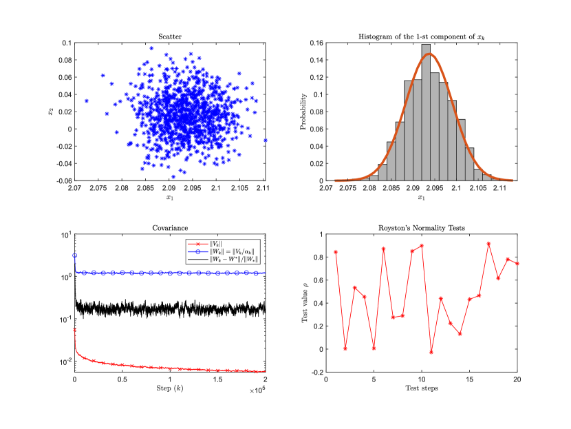
Figure 1: (Color Online). Numerical simulation of vSGD with $a=0.25$. Top left: Scatter plot of the first two components of $\{x_{k}\}$ after $2\times 10^{5}$ steps. Top right: The distribution of the first component of $\{x_{k}\}$ after $2\times 10^{5}$ steps. Bottom Left: $\|V_{k}\|=\|\mathbb{E}(x_{k}x_{k}^{T})\|$ (red stars), $\|W_{k}\|=\|\mathbb{E}(x_{k}x_{k}^{T})/\alpha_{k}\|$ (blue circles) and relative error $\|W_{k}-W^{*}\|/\|W^{*}\|$ (black line). Bottom right: Test values $\rho$ per $10^{4}$ steps.

In this section, we will present numerical experiments for a toy model to validate the theoretical analysis for the CLT for the SGD-type methods.

We consider a logistic regression problem, i.e., the finite sum with penalty function, $\mu$-strongly convex function

$$f(x)=\frac{1}{N}\sum_{i=1}^{n}\left[\ln(1+e^{w_{i}^{T}x})-y_{i}w_{i}^{T}x\right]+\frac{\beta}{2}\|x\|^{2},x\in\mathbb{R}^{d}$$

By computing, we have

$$\nabla f(x)=\frac{1}{N}\sum_{i=1}^{n}\left[\frac{w_{i}}{1+e^{w_{i}^{T}x}}+(1-y_{i})w_{i}\right]+\beta x,\nabla^{2}f(x)=\frac{1}{N}\sum_{i=1}^{n}\left[\frac{w_{i}w_{i}^{T}e^{w_{i}^{T}x}}{(1+e^{w_{i}^{T}x})^{2}}\right]+\beta I.$$

In the following numerical experiments, we choose learning rates $\alpha_{k}=0.1\cdot k^{-a}$ and $\beta=0.05$, $d=10$, the batch size is 1.

Test of vSGD

We choose the sample size $M=1000$ in the simulation of vSGD with learning rates $\alpha_{k}=0.1\cdot k^{-0.25}$, and make statistical plots after $2\times 10^{5}$ steps (Figure 1).

The top left panel of Figure 1 shows the scatter plot of $\{x_{k}\}$ at the final simulation step. The top right panel shows the distribution of the first component of $\{x_{k}\}$ at the final simulation step, which perfectly fits a normal distribution. Other components of $\{x_{k}\}$ shows similar behavior, which is omitted here. To check whether $W_{k}=\mathbb{E}x_{k}x_{k}^{T}/\alpha_{k}\rightarrow W^{*}$, we first present the results to show how $W_{k}$ change with the number of iterations in the bottom left panel of Figure 1, which demonstrates convergence in a very early stage of iterations. To further quantify how far $W_{k}$ is from $W^{*}$, we utilize different sample sizes $M=100,250,500,1000,2000$ and learning schedules $\alpha_{k}=k^{-a}$ with $a=0.25,0.50,0.75$ to make the study, and the results are shown in Table 1. To understand its meaning, we note that we indeed use $\tilde{W}_{k}=\sum_{m=1}^{M}x_{k}(\omega_{m})x_{k}^{T}(\omega_{m})/(M\alpha_{k})$ to approximate $W_{k}=\mathbb{E}x_{k}x_{k}^{T}/\alpha_{k}$, and we have the bias-variance error decomposition

$$\tilde{W}_{k}-W^{*}=\tilde{W}_{k}-W_{k}+W_{k}-W^{*}\sim O(M^{-1/2})+O(k^{a-1}).$$

When $a$ is relatively small ($a=0.25,0.5$ in Table 1), the bias error can be neglected and we may expect the decay ratio $\sqrt{2}/2$ when $M$ is doubled. This can be exactly observed in the cases $a=0.25,0.5$. However, when $a=0.75$, the bias error is not that small compared with the sampling error, and we can not get such perfect scaling behavior although the error decays with the increasing sample size.

Figure 2: (Color Online). Numerical simulation of mSGD with $a=0.5$ and $\mu=0.2$. Top left: Scatter plot of the first components of $\{x_{k}\}$ and $\{v_{k}\}$ after $2\times 10^{5}$ steps. Top right: Distribution of the first component of $\{Z_{k}\}$ after $2\times 10^{5}$ steps. Bottom left: $\|V_{k}\|=\|\mathbb{E}(Z_{k}Z_{k}^{T})\|$ (red stars), $\|W_{k}\|=\|\mathbb{E}(Z_{k}Z_{k}^{T})/\alpha_{k}\|$ (blue circles) and relative error $\|W_{k}-W^{*}\|/\|W^{*}\|$ (black line). Bottom right: Test values $\rho$ per $10^{4}$ steps.

Table 1: Relative error $\|\tilde{W}_{k}-W^{*}\|/\|W^{*}\|$ for vSGD with different sample sizes $M$ and learning rates $\alpha_{k}=k^{-a}$.

Sample size $M$	100	250	500	1000	2000
$a=0.25$	0.122	0.0761	0.0545	0.0385	0.0274
$a=0.50$	0.123	0.0791	0.0535	0.0400	0.0268
$a=0.75$	0.151	0.102	0.0957	0.0808	0.0646

To further quantitatively check $\mathrm{Cov}(x_{k})^{-1/2}x_{k}\rightarrow N(0,1)$, we use Royston’s multivariate normality test [24] to check whether $\{x_{k}\}$ is normally distributed at the $k$th simulation step. The test value is $\rho=p-\sigma$, where $p$ is the $p$-value associated with the Royston’s statistic and $\sigma$ is the given significance ($\sigma=0.05$ in the experiments). The value $\rho>0$ indicates that $\{x_{k}\}$ passes the normal distribution test. The bottom right panel of Figure 1 shows the value of $\rho$ per $10^{4}$ steps, which clearly verifies $\mathrm{Cov}(x_{k})^{-1/2}x_{k}\rightarrow N(0,1).$

Test of mSGD

We also choose $M=2000$ samples in the simulation of mSGD with learning rates $\alpha_{k}=0.1\cdot k^{-a}$ to verify our CLT results after $5\times 10^{5}$ iteration steps (Figure 2).

We perform simulations using the mSGD method with constant damping $\mu=0.2$ and learning rates $\alpha_{k}=0.1\cdot k^{-0.5}$. The corresponding statistical plots are shown in Figure 2, and similar insights can be gained as the vSGD case. The top left panel shows the scatter plot of $\{x_{k}\}$ and $\{v_{k}\}$ at the final simulation step. The top right panel shows the distribution of the first component of $\{Z_{k}\}$ at the final simulation step. To verify $W_{k}=\mathbb{E}x_{k}x_{k}^{T}/\alpha_{k}\rightarrow W^{*}$, we present the results to show how $W_{k}$ change with the number of iterations in bottom left panel of Figure 2. Since the eigenvalues of $D$ are complex-valued, the oscillatory relaxation can be observed in the convergence process. The bottom right panel shows the value of $\rho$ per $10^{4}$ steps. The positive values of $\rho$ suggest $\mathrm{Cov}(Z_{k})^{-1/2}Z_{k}\rightarrow N(0,1).$

We also perform simulations using the mSGD method with vanishing damping $\mu_{k}=k^{-0.15}$ and learning rates $\alpha_{k}=0.5\cdot k^{-0.75}$. The numerical results again support our theoretical analysis $\mathrm{Cov}(Z_{k})^{-1/2}Z_{k}\rightarrow N(0,1)$, and they pass the normality test well. However, we will omit it due to the limit of space.

7 Conclusion

In this article, we re-established the CLT of vSGD under more general learning rates conditions. We also studied the mSGD and NaSGD with constant damping $\mu_{k}\equiv\tilde{\mu}$ and vanishing damping $\mu_{k}\rightarrow 0$ by taking advantage of the Lyapunov function technique, which are not previously known. The CLT for the time average was also investigated, and we found that the CLT for the time average held in the linear case, while it was not true in general nonlinear situation. Numerical tests were carried out to verify the theoretical analysis. Applications and further extensions of the results obtained in this paper will be of future interest.

8 Appendix: Proof of Lemmas in the main text

8.1 Proof of Lemma 3.1

The proof of Lemma 3.1 relies on the following lemma.

Lemma 8.1.

Assume the learning rates $\{\alpha_{k}\}$ satisfy Assumption (A1) and the positive sequence $\beta_{k}\rightarrow 0$. Consider the triplet $(z_{k},\beta_{k},c)$ with the relation

$$z_{k}\leq(1-c\alpha_{k})z_{k-1}+\alpha_{k}\beta_{k},\qquad z_{k},c>0.$$ (71)

We have: (a) $z_{k}\rightarrow 0$. Further assume there exists $M>0$, such that $\beta_{n}\geq M\prod_{k=m+1}^{n}(1-h\alpha_{k})\beta_{m}$, for any $n>m$, where $\beta_{k}$ satisfies the $h$-slow condition with $h<c$. Then we have: (b) $z_{n}\leq K\beta_{n}$, where $K>0$ is a constant.

Proof.

Proof of Lemma 8.1 To establish (a), we first assume $\sup_{k}\alpha_{k}<c^{-1}$ without loss of generality. Let $B_{n}=\prod_{k=1}^{n}(1-c\alpha_{k})$, we have

$$z_{n}\leq\sum_{k=1}^{n}B_{n}B_{k}^{-1}\alpha_{k}\beta_{k}+B_{n}z_{0}.$$

By $B_{n}B_{k}^{-1}c\alpha_{k}=B_{n}B_{k}^{-1}-B_{n}B_{k-1}^{-1}$, we get $\sum_{k=1}^{n}B_{n}B_{k}^{-1}\alpha_{k}\rightarrow c^{-1}.$

Let $\gamma_{n}=\sup_{k\geq n}{\beta_{k}},$ then for large enough $m,n$ and $m<n$, we have

$$z_{n}\leq B_{n}B_{m}^{-1}z_{m}+\sum_{k=m+1}^{n}B_{n}B_{k}^{-1}\alpha_{k}\gamma_{m}\leq c^{-1}\gamma_{m}+B_{n}B_{m}^{-1}z_{m}.$$

Taking $m=0,$ we obtain that $\{z_{k}\}$ is bounded. Then for any $\varepsilon>0$, there exists $M>0$, such that $\gamma_{m}<c\varepsilon/2$, for any $m>M$. And there exists $N>0$, such that $B_{n}B_{k}^{-1}<\varepsilon/2$, for any $m>N$, which gives $z_{k}\rightarrow 0.$

For (b), letting $C_{n}=\prod_{k=1}^{n}(1-c\alpha_{k})(1-h\alpha_{k})^{-1}$, we get $\sum_{k=1}^{n}\alpha_{k}C_{n}C_{k}^{-1}\rightarrow(c-h)^{-1}$. By

$$z_{n}\leq\sum_{k=1}^{n}C_{n}C_{k}^{-1}\alpha_{k}\beta_{n}+B_{n}z_{0}$$

and $B_{n}z_{0}\rightarrow 0$, we obtain that there exists a constant $K>0$ such that $z_{n}\leq K\beta_{n}$. ∎

The same result can be obtained if condition (71) is replaced with

$$z_{k}\leq(1-c\alpha_{k}+o(\alpha_{k}))z_{k-1}+\alpha_{k}\beta_{k}.$$

Proof.

Proof of Lemma 3.1 Consider the Lyapunov equation $D^{T}W+WD=Q$ with $Q\succ 0,W\succ 0$. There exists $c>0$, such that $Q/2\succ 2cW$. We have

$$A_{m}^{-T}A_{n}^{T}WA_{n}A_{m}^{-1} =A_{m}^{-T}A_{n-1}^{T}\left(W-\alpha_{n}\left(D^{T}W+WD\right)+o\left(\alpha_{n}\right)\right)A_{n-1}A_{m}^{-1}$$

$$\preceq A_{m}^{-T}A_{n-1}^{T}\left(W-\alpha_{n}Q+o\left(\alpha_{n}\right)\right)A_{n-1}A_{m}^{-1}$$

$$\preceq A_{m}^{-T}A_{n-1}^{T}(W+o\left(\alpha_{n}\right))A_{n-1}A_{m}^{-1}-A_{m}^{-T}A_{n-1}^{T}QA_{n-1}A_{m}^{-1}\frac{\alpha_{n}}{2}$$

$$\preceq\left(1-2c\alpha_{n}\right)A_{m}^{-T}A_{n-1}^{T}WA_{n-1}A_{m}^{-1},$$

where $m,n$ are large enough and $m<n$. We can get

$$A_{m}^{-T}A_{n}^{T}WA_{n}A_{m}^{-1}\preceq\prod_{k=m+1}^{n}\left(1-2c\alpha_{k}\right)W,$$

which gives

$$\left\|A_{m}^{-T}A_{n}^{T}WA_{n}A_{m}^{-1}\right\|_{2}\leq K\prod_{k=m+1}^{n}\left(1-2c\alpha_{k}\right),$$

where $K=\lambda_{\max}(W)$. So we have

$$\left\|\sum_{k=1}^{n}A_{n}A_{k}^{-1}WA_{k}^{-T}A_{n}^{T}\alpha_{k}\beta_{k}\right\|_{2}\leq K\sum_{k=1}^{n}\prod_{i=k+1}^{n}\left(1-2c\alpha_{i}\right)\alpha_{k}\left|\beta_{k}\right|.$$

Let $z_{n}=\sum_{k=1}^{n}\prod_{i=k+1}^{n}\left(1-2c\alpha_{i}\right)\alpha_{k}\left|\beta_{k}\right|$ and consider the triplet $\left(z_{k},\left|\beta_{k}\right|,2c\right)$ in Lemma 8.1, then we know that $z_{n}\rightarrow 0$, which means

$$\sum_{k=1}^{\infty}A_{n}A_{k}^{-1}WA_{k}^{-T}A_{n}^{T}\alpha_{k}\beta_{k}\rightarrow 0.$$

The proof is completed. ∎

8.2 Proof of Lemma 3.2

Proof.

Proof of Lemma 3.2 We will separate the cases $p=1$ and $p>1$.

Case $p=1$. By the $L$-smoothness and $\mu$-strong convexity of $f$, we have

$$\begin{split}\mathbb{E}\|X_{k}\|^{2}&\leq\mathbb{E}\|X_{k-1}\|^{2}-2\alpha_{k}X_{k}^{T}\nabla f(x_{k-1})+\alpha_{k}^{2}(1+K_{\xi})\|\nabla f(x_{k-1})\|^{2}+M\alpha_{k}^{2}\\ &\leq\big{(}1-2\mu\alpha_{k}+(1+K_{\xi})L^{2}\alpha_{k}^{2}\big{)}\mathbb{E}\|X_{k-1}\|^{2}+M\alpha_{k}^{2}.\end{split}$$

Now take the triplet $(\mathbb{E}\|X_{k}\|^{2},M\alpha_{k},2\mu)$ in Lemma 8.1. We get $\mathbb{E}\|X_{k}\|^{2}\rightarrow 0.$ And with the $h_{0}$-slow condition of $\alpha_{k}$, we know that there exists $C>0$, such that $\mathbb{E}\|X_{k}\|^{2}\leq C\alpha_{k}$.

Case $p>1$. Define $Y_{k-1}=X_{k-1}-\alpha_{k}\nabla f(x_{k-1})$. Through $\mu$-strongly convex and $L$-smooth condition of $f$, we have

$$\begin{split}\|Y_{k-1}\|^{2p}&=\big{(}\|X_{k-1}\|^{2}-2\alpha_{k}X_{k-1}^{T}\nabla f(x_{k-1})+\alpha_{k}^{2}\|\nabla f(x_{k-1})\|^{2}\big{)}^{p}\\ &\leq\|X_{k-1}\|^{2p}(1-2\mu\alpha_{k}+L^{2}\alpha_{k}^{2})^{p}.\end{split}$$

For $p\leq 1+\frac{\delta_{0}}{2}$, we have

$$\mathbb{E}\|\xi_{k}\|^{2p}\leq M_{p}+V_{p}\mathbb{E}\|\nabla f(x_{k-1})\|^{2p}\leq M_{p}+V_{p}L^{2p}\mathbb{E}\|X_{k-1}\|^{2p}$$

by Assumption (15). By the inequality $(a+b)^{p}\leq a^{p}+2^{p-1}p(a^{p-1}b+b^{p})$ for $p>1$ and $a,b>0$, we get

$$\begin{split}\quad\mathbb{E}\|X_{k}\|^{2p}&=\mathbb{E}\|Y_{k-1}+\alpha_{k}\xi_{k}\|^{2p}=\mathbb{E}|Y_{k-1}^{T}Y_{k-1}+2\alpha_{k}\xi_{k}^{T}Y_{k-1}+\alpha_{k}^{2}\xi_{k}^{T}\xi_{k}|^{p}\\ &\leq C\big{\{}\mathbb{E}(\|\xi_{k}\|^{2}|Y_{k-1}^{T}Y_{k-1}+2\alpha_{k}\xi_{k}^{T}Y_{k-1}|^{p-1})\alpha_{k}^{2}+\mathbb{E}\|\xi_{k}\|^{2p}\alpha_{k}^{2p}\big{\}}\\ &~{}~{}~{}~{}+\mathbb{E}|Y_{k-1}^{T}Y_{k-1}+2\alpha_{k}\xi_{k}^{T}Y_{k-1}|^{p}.\end{split}$$

Define $q=p/(p-1)$. By using Hölder’s inequality, for $\varepsilon_{1}>0$, we have

$$\mathbb{E}\big{(}\|\xi_{k}\|^{2}|Y_{k-1}^{T}Y_{k-1}+2\alpha_{k}\xi_{k}^{T}Y_{k-1}|^{p-1}\big{)}\alpha_{k}^{2}\leq\alpha_{k}\Big{(}\frac{\varepsilon_{1}}{q}\mathbb{E}|Y_{k-1}^{T}Y_{k-1}+2\alpha_{k}\xi_{k}^{T}Y_{k-1}|^{p}+\frac{\alpha_{k}^{p}}{p\varepsilon_{1}^{p-1}}\mathbb{E}\|\xi_{k}\|^{2p}\Big{)},$$

which means

$$\mathbb{E}\|X_{k}\|^{2p}\leq(1+C\varepsilon_{1}\alpha_{k})\mathbb{E}|Y_{k-1}^{T}Y_{k-1}+2\alpha_{k}\xi_{k}^{T}Y_{k-1}|^{p}+C\alpha_{k}^{p+1}\mathbb{E}\|\xi_{k}\|^{2p}.$$

By Hölder’s inequality and $(a+b)^{p}\leq a^{p}+pa^{p-1}b+D_{p}(a^{p-2}b^{2}+b^{p})$ for $p>1$ and $a,b>0$, where $D_{p}=2^{p-2}p(p-1)$, for any $\varepsilon_{2},~{}\varepsilon_{3}>0,$ we have

$$\begin{split}&\quad\ \mathbb{E}\big{|}Y_{k-1}^{T}Y_{k-1}+2\alpha_{k}\xi_{k}^{T}Y_{k-1}\big{|}^{p}\\ &\leq\mathbb{E}\|Y_{k-1}\|^{2p}+p\mathbb{E}(\xi_{k}^{T}Y_{k-1}\|Y_{k-1}\|^{2p-2})+D_{p}\big{(}\alpha_{k}^{2}\mathbb{E}(\|\xi_{k}\|^{2}\|Y_{k-1}\|^{2p-2})+\alpha_{k}^{p}\mathbb{E}(\|\xi_{k}\|^{p}\|Y_{k-1}\|^{p})\big{)}\\ &\leq\mathbb{E}\|Y_{k-1}\|^{2p}+C\alpha_{k}\left(\mathbb{E}\frac{\alpha_{k}^{p}\|\xi_{k}\|^{2p}}{\varepsilon_{2}^{p-1}}+\varepsilon_{2}\mathbb{E}\|Y_{k-1}\|^{2p}\right)+C\alpha_{k}^{p-1}\left(\mathbb{E}\frac{\alpha_{k}^{p}\|\xi_{k}\|^{2p}}{\varepsilon_{3}}+\varepsilon_{3}\mathbb{E}\|Y_{k-1}\|^{2p}\right)\\ &\leq(1+C(\varepsilon_{2}+\varepsilon_{3})\alpha_{k})\mathbb{E}\|Y_{k-1}\|^{2p}+C\alpha_{k}^{p+1}\mathbb{E}\|\xi_{k}\|^{2p}.\end{split}$$

Then we get

$$\mathbb{E}\|X_{k}\|^{2p}\leq(1+C\varepsilon_{1}\alpha_{k})(1+C(\varepsilon_{2}+\varepsilon_{3})\alpha_{k})(1-2\mu\alpha_{k}+L^{2}\alpha_{k}^{2})^{p}\mathbb{E}\|X_{k-1}\|^{2p}+C(1+\mathbb{E}\|X_{k-1}\|^{2p})\alpha_{k}^{p+1}.$$

By the arbitrariness of $\varepsilon_{1},\varepsilon_{2},\varepsilon_{3}$, we have

$$\begin{split}\mathbb{E}\|X_{k}\|^{2p}\leq(1-(2\mu-\varepsilon)p\alpha_{k}+o(\alpha_{k}))\mathbb{E}\|X_{k-1}\|^{2p}+C\alpha_{k}^{p+1}\end{split}$$

for any $0<\varepsilon<2\mu$. Now take the triplet $(\mathbb{E}\|X_{k}\|^{2p},C\alpha_{k}^{p},2\mu-\varepsilon)$ in Lemma 8.1, we have

$$\begin{split}\mathbb{E}\|X_{k}\|^{2p}\leq U_{p}\alpha_{k}^{p}\end{split}$$

with $U_{p}>0$, which gives the upper bounds of $X_{k}$ in $L^{2p}$ for $p\in[1,1+\delta_{0}/2]$. ∎

8.3 $L^{2p}$ bounds for mSGD with constant damping $\mu_{k}\equiv\tilde{\mu}$

Proof.

Proof For mSGD, we first consider the case $p=1$. Define the Hamiltonian $H_{k}=f(x_{k})-f(x^{*})+\|v_{k}\|^{2}/2$ and $\bar{H}_{k}=\|\nabla f(x_{k})\|^{2}+\|v_{k}\|^{2}$.

By (42) and $L$-smoothness of $f$ and $\mathbb{E}[\|\xi_{k}\|^{2}|\mathcal{F}_{k-1}]\leq M+K_{\xi}\|\nabla f(x_{k-1})\|^{2}$, we have

$$\begin{split}\mathbb{E}[f(x_{k})|\mathcal{F}_{k-1}]&\leq f(x_{k-1})+\alpha_{k}\mathbb{E}[\nabla f(x_{k-1})^{T}v_{k}|\mathcal{F}_{k-1}]+\frac{L\alpha_{k}^{2}}{2}\mathbb{E}[\|v_{k}\|^{2}|\mathcal{F}_{k-1}]\\ &\leq f(x_{k-1})+\alpha_{k}\nabla f(x_{k-1})^{T}v_{k-1}+C\alpha_{k}^{2}(1+O(\bar{H}_{k-1})),\end{split}$$

and

$$\begin{split}\mathbb{E}\Big{[}\frac{\|v_{k}\|^{2}}{2}|\mathcal{F}_{k-1}\Big{]}&\leq\frac{\|v_{k-1}\|^{2}}{2}+\frac{1}{2}\mathbb{E}[\|v_{k}-v_{k-1}\|^{2}|\mathcal{F}_{k-1}]-\alpha_{k}\left(\tilde{\mu}\|v_{k-1}\|^{2}+\nabla f(x_{k-1})v_{k-1}\right)\\ &\leq\frac{\|v_{k-1}\|^{2}}{2}-\alpha_{k}(\tilde{\mu}\|v_{k-1}\|^{2}+\nabla f(x_{k-1})v_{k-1})+C\alpha_{k}^{2}(1+O(\bar{H}_{k-1})),\end{split}$$

thus

$$\begin{split}\mathbb{E}[H_{k}|\mathcal{F}_{k-1}]&\leq H_{k-1}-\tilde{\mu}\alpha_{k}\|v_{k-1}\|^{2}+C\alpha_{k}^{2}(1+O(\bar{H}_{k-1})).\end{split}$$

By introducing the term $\tilde{Z}_{k}=v_{k}^{T}\nabla f(x_{k})$, with $L$-smoothness of $f$, we get

$$\begin{split}\mathbb{E}[\tilde{Z}_{k}|\mathcal{F}_{k-1}]&=\tilde{Z}_{k-1}+\mathbb{E}[v_{k}^{T}(\nabla f(x_{k})-\nabla f(x_{k-1}))|\mathcal{F}_{k-1}]+\mathbb{E}[(v_{k}-v_{k-1})^{T}\nabla f(x_{k-1})|\mathcal{F}_{k-1}]\\ &\leq\tilde{Z}_{k-1}+\alpha_{k}(L\mathbb{E}[\|v_{k}\|^{2}|\mathcal{F}_{k-1}]-\|\nabla f(x_{k-1})\|^{2}-\tilde{\mu}v_{k-1}^{T}\nabla f(x_{k-1}))\\ &=\tilde{Z}_{k-1}+\alpha_{k}(L\|v_{k-1}\|^{2}-\|\nabla f(x_{k-1})\|^{2}-\tilde{\mu}v_{k-1}^{T}\nabla f(x_{k-1}))\\ &\quad+\alpha_{k}^{2}(O(\bar{H}_{k-1})+o(1)).\end{split}$$

Now we consider the Lyapunov function $H^{E}_{k}=\mathbb{E}\tilde{H}_{k}$ with $\tilde{H}_{k}=H_{k}+\zeta\tilde{Z}_{k}$, where $\zeta>0$ is small enough. From the $L$-smoothness and strong convexity of $f$, we have $\tilde{H}_{k}=\Theta(\bar{H}_{k})$. Then

$$\begin{split}&\mathbb{E}[\tilde{H}_{k}|\mathcal{F}_{k-1}]\leq\tilde{H}_{k-1}-\alpha_{k}F_{k-1}+C\alpha_{k}^{2}(1+O(\tilde{H}_{k-1})),\end{split}$$

where $F_{k-1}=\zeta\|\nabla f(x_{k-1})+\frac{\tilde{\mu}}{2}v_{k-1}\|^{2}+(\tilde{\mu}-\zeta(\frac{\tilde{\mu}^{2}}{4}+L))\|v_{k-1}\|^{2}$. Since $f$ is strongly convex, it is easy to get $F_{k}=\Theta(\bar{H}_{k})$, which means that there exists $K>0$ such that

$$\begin{split}\mathbb{E}[\tilde{H}_{k}|\mathcal{F}_{k-1}]&\leq(1-K\alpha_{k}+o(\alpha_{k}))\tilde{H}_{k-1}+C\alpha_{k}^{2}.\end{split}$$

Then we have

$$\begin{split}H^{E}_{k}&\leq(1-K\alpha_{k}+o(\alpha_{k}))H^{E}_{k-1}+C\alpha_{k}^{2}.\end{split}$$

Taking the triplet as $(H^{E}_{k},C\alpha_{k},K)$ in Lemma 8.1, we have $H^{E}_{k}\leq U_{1}\alpha_{k}$, where $U_{1}>0$. Then the $L^{2}$ bound for mSGD is obtained as a result of $\mathbb{E}\|Z_{k}\|^{2}\leq CH^{E}_{k}$.

The estimate for $p\in[1,1+\delta_{0}/2]$ is similar to the derivations in Appendix 8.2 for vSGD and we omit it. ∎

8.4 $L^{2p}$ bounds for NaSGD with constant damping $\mu_{k}\equiv\tilde{\mu}$

Proof.

Proof The analysis for NaSGD is similar to mSGD. For $p=1$, we consider the Hamiltonian $H_{k}=f(x_{k})-f(x^{*})+\|v_{k}\|^{2}/2$. Let $\bar{H}_{k}=\|\nabla f(x_{k})\|^{2}+\|v_{k}\|^{2}$. By (49) with $y_{k-1}=x_{k-1}+\beta_{k}v_{k-1}$, we have

$$\begin{split}\mathbb{E}[H_{k}|\mathcal{F}_{k-1}]&\leq H_{k-1}+\alpha_{k}[v_{k-1}^{T}(\nabla f(x_{k-1})-\nabla f(y_{k-1}))-\tilde{\mu}\|v_{k-1}\|^{2}]+o(\alpha_{k})\\ &\leq H_{k-1}-(\tilde{\mu}+\mu\beta_{k})\alpha_{k}\|v_{k-1}\|^{2}+C\alpha_{k}^{2}(1+O(\bar{H}_{k-1})).\end{split}$$

And for $\tilde{Z}_{k}=v_{k}^{T}\nabla f(x_{k})$, we have

$$\begin{split}\mathbb{E}[\tilde{Z}_{k}|\mathcal{F}_{k-1}]&\leq Z_{k-1}+\alpha_{k}(L\|v_{k-1}\|^{2}-\nabla f(x_{k-1})^{T}\nabla f(y_{k-1})-\tilde{\mu}v_{k-1}^{T}\nabla f(x_{k-1}))+\alpha_{k}^{2}O(\bar{H}_{k-1}).\end{split}$$

By $L$-smoothness of $f$, we get

$$|\nabla f(x_{k-1})^{T}(\nabla f(x_{k-1})-\nabla f(y_{k-1}))|\leq L\beta_{k}|v_{k-1}^{T}\nabla f(x_{k-1})|\leq\hat{\beta}L\lambda\|\nabla f(x_{k-1})\|^{2}+\frac{\hat{\beta}L}{\lambda}v_{k-1}^{2},$$

where $\hat{\beta}=\sup_{k}\beta_{k}$ and $\lambda=1/(2L\hat{\beta})$. Then we have

$$\begin{split}\mathbb{E}[\tilde{Z}_{k}|\mathcal{F}_{k-1}]&\leq Z_{k-1}+\alpha_{k}\Big{(}(L+\frac{L\hat{\beta}}{\lambda})\|v_{k-1}\|^{2}-(1-L\hat{\beta}\lambda)\|\nabla f(x_{k-1})\|^{2}-\tilde{\mu}v_{k-1}^{T}\nabla f(x_{k-1})\Big{)}\\ &+C\alpha_{k}^{2}(1+O(\bar{H}_{k-1})).\end{split}$$

Now we consider the Lyapunov function $H^{E}_{k}=\mathbb{E}\tilde{H}_{k}=\mathbb{E}(H_{k}+\zeta\tilde{Z}_{k})$ with small enough $\zeta>0$. Similar to analysis of mSGD in Appendix 8.3, we have

$$H^{E}_{k}\leq(1-K\alpha_{k}+o(\alpha_{k}))H^{E}_{k-1}+C\alpha_{k}^{2}.$$

The rest analysis is similar to the derivations in Appendix 8.3. ∎

8.5 Proof of Lemma 4.2

Proof.

Proof of Lemma 4.2 For mSGD with $\mu_{k}\rightarrow 0$, consider the Lyapunov function $H^{E}_{k}=\mathbb{E}\tilde{H}_{k}$, where $\tilde{H}_{k}=H_{k}+\lambda\mu_{k}\tilde{Z}_{k},$ with $0<\lambda<1/L$. From the $L$-smoothness and strong convexity of $f$, we have $\tilde{H}_{k}=\Theta(\bar{H}_{k})$. Similar to mSGD, we have

$$\begin{split}\mathbb{E}[\tilde{H}_{k}|\mathcal{F}_{k-1}]&\leq\tilde{H}_{k-1}-\alpha_{k}\tilde{F}_{k-1}-\lambda(\mu_{k}-\mu_{k-1})v_{k-1}^{T}\nabla f(x_{k-1})+C(1+O(\bar{H}_{k-1}))\alpha_{k}^{2},\end{split}$$

where $\tilde{F}_{k-1}=\lambda\mu_{k}(\|\nabla f(x_{k-1})\|^{2}+v_{k-1}^{T}\nabla f(x_{k-1}))+(1-L\lambda)\mu_{k}\|v_{k-1}\|^{2}.$

Further, let $\lambda<(L+L_{\mu}^{2}/4)^{-1}$. By (54), we have $\tilde{F}_{k}+\lambda(\mu_{k+1}-\mu_{k})\tilde{Z}_{k}=\mu_{k+1}\Theta(\bar{H}_{k})$. Similar to the analysis of mSGD in Appendix 8.3, there exists $K>0$ such that

$$\begin{split}\mathbb{E}[\tilde{H}_{k}|\mathcal{F}_{k-1}]&\leq(1-K\alpha_{k}\mu_{k}+o(\alpha_{k}\mu_{k}))\tilde{H}_{k-1}+C(1+O(\tilde{H}_{k-1}))\alpha_{k}^{2}.\\ \end{split}$$

Then we have

$$H^{E}_{k}\leq(1-K\alpha_{k}\mu_{k}+o(\alpha_{k}\mu_{k}))H^{E}_{k-1}+C\alpha_{k}^{2}.$$

Taking the triplet as $(H^{E}_{k},C\alpha_{k}/\mu_{k},K)$ and using $\{\alpha_{k}\mu_{k}\}$ instead of $\{\alpha_{k}\}$ in Lemma 8.1, we have $H^{E}_{k}\leq C\alpha_{k}/\mu_{k}$.

The estimate for $p\in[1,1+\delta_{0}/2]$ is also similar to the derivations in Appendix 8.2. ∎

References

- [1] M. Assran and M. Rabbat. On the convergence of Nesterov’s accelerated gradient method in stochastic settings. In Proceedings of the 37th International Conference on Machine Learning, volume 119 of Proceedings of Machine Learning Research, pages 410–420. PMLR, 13–18 Jul 2020.
- [2] A. Barakat and P. Bianchi. Convergence rates of a momentum algorithm with bounded adaptive step size for nonconvex optimization. In Proceedings of The 12th Asian Conference on Machine Learning, volume 129 of Proceedings of Machine Learning Research, pages 225–240. PMLR, 18–20 Nov 2020.
- [3] D. P. Bertsekas and J. N. Tsitsiklis. Gradient convergence in gradient methods with errors. SIAM Journal on Optimization, 10(3):627–642, 2000.
- [4] V. S. Borkar. Stochastic approximation: a dynamical systems viewpoint, volume 48. Springer, 2009.
- [5] L. Bottou, F. E. Curtis, and J. Nocedal. Optimization methods for large-scale machine learning. SIAM Review, 60(2):223–311, 2018.
- [6] H. Chen. Stochastic Approximation and Its Applications. Kluwer Academic Press, New York, 2003.
- [7] S. Ghadimi and G. Lan. Stochastic first- and zeroth-order methods for nonconvex stochastic programming. SIAM Journal on Optimization, 23(4):2341–2368, 2013.
- [8] P. Hall and C. C. Heyde. Martingale limit theory and its application. Academic press, New York, 1980.
- [9] R. Jin, Y. Xing, and X. He. On the convergence of msgd and adagrad for stochastic optimization. arXiv preprint arXiv:2201.11204, 2022.
- [10] V. R. Konda and J. N. Tsitsiklis. Convergence rate of linear two-time-scale stochastic approximation. The Annals of Applied Probability, 14(2):796–819, 2004.
- [11] J. Lei and U. V. Shanbhag. Variance-reduced accelerated first-order methods: Central limit theorems and confidence statements. arXiv preprint arXiv:2006.07769, 2020.
- [12] Y. Liu, Y. Gao, and W. Yin. An improved analysis of stochastic gradient descent with momentum. Advances in Neural Information Processing Systems, 33:18261–18271, 2020.
- [13] E. Moulines and F. Bach. Non-asymptotic analysis of stochastic approximation algorithms for machine learning. Advances in neural information processing systems, 24, 2011.
- [14] Y. Nesterov. A method for solving the convex programming problem with convergence rate . Proceedings of the USSR Academy of Sciences, 269:543–547, 1983.
- [15] Y. Nesterov. Introductory Lectures on Convex Optimization. Kluwer Academic Publishers, New York, 2004.
- [16] L. M. Nguyen, P. H. Nguyen, P. Richtárik, K. Scheinberg, M. Takáč, and M. van Dijk. New convergence aspects of stochastic gradient algorithms. Journal of Machine Learning Research, 20(176):1–49, 2019.
- [17] B. T. Polyak. Some methods of speeding up the convergence of iteration methods. USSR Computational Mathematics and Mathematical Physics, 4(5):1–17, 1964.
- [18] B. T. Polyak and A. B. Juditsky. Acceleration of stochastic approximation by averaging. SIAM Journal on Control and Optimization, 30(4):838–855, 1992.
- [19] S. J. Reddi, A. Hefny, S. Sra, B. Poczos, and A. Smola. Stochastic variance reduction for nonconvex optimization. In Proceedings of The 33rd International Conference on Machine Learning, volume 48 of Proceedings of Machine Learning Research, pages 314–323. PMLR, 20–22 Jun 2016.
- [20] C. Robert and G. Casella. Monte Carlo Statistical Methods. Springer Science & Business Media, New York, 2nd edition edition, 2004.
- [21] J. Sirignano and K. Spiliopoulos. Stochastic gradient descent in continuous time: A central limit theorem. Stochastic Systems, 10(2):124–151, 2020.
- [22] W. Su, S. Boyd, and E. J. Candès. A differential equation for modeling nesterov’s accelerated gradient method: Theory and insights. Journal of Machine Learning Research, 17(153):1–43, 2016.
- [23] Y. W. Teh, A. H. Thiery, and S. J. Vollmer. Consistency and fluctuations for stochastic gradient langevin dynamics. Journal of Machine Learning Research, 17(7):1–33, 2016.
- [24] A. Trujillo-ortiz, R. Hernandez-Walls, K. Barba-Rojo, and L. Cupul-Magana. Roystest. royston’s multivariate normality test. URL http://www. mathworks. com/matlabcentral/fileexchange/17811, 2007.
- [25] S. Varadhan. Probability Theory. American Mathematical Society, Providence, 2001.