Can we achieve robustness from data alone?

Abstract

We introduce a meta-learning algorithm for adversarially robust classification. The proposed method tries to be as model agnostic as possible and optimizes a dataset prior to its deployment in a machine learning system, aiming to effectively erase its non-robust features. Once the dataset has been created, in principle no specialized algorithm (besides standard gradient descent) is needed to train a robust model. We formulate the data optimization procedure as a bi-level optimization problem on kernel regression, with a class of kernels that describe infinitely wide neural nets (Neural Tangent Kernels). We present extensive experiments on standard computer vision benchmarks using a variety of different models, demonstrating the effectiveness of our method, while also pointing out its current shortcomings. In parallel, we revisit prior work that also focused on the problem of data optimization for robust classification (Ilyas et al., 2019), and show that being robust to adversarial attacks after standard (gradient descent) training on a suitable dataset is more challenging than previously thought.

1 Introduction

The discovery of the adversarial vulnerability of neural nets (Szegedy et al., 2014; Goodfellow et al., 2015; Papernot et al., 2017; Carlini & Wagner, 2017) - their brittleness when exposed to imperceptible perturbations in the data - has shifted the focus of the machine learning community from standard gradient techniques to more complex training algorithms that are rooted in robust optimization. In principle, if $\mathcal{P}$ denotes a data distribution and $\Delta$ is a set of allowed perturbations of the input space, we would like to solve the following problem (Madry et al., 2018):

$$\inf_{\theta}\mathbb{E}_{(x,y)\sim\mathcal{P}}\sup_{\delta\in\Delta}\mathcal{L}(f(x+\delta;\theta,\mathcal{D}_{\mathrm{train}}),y),$$ (1)

where $f$ is a model parameterized by $\theta$ (e.g. a neural network), $\mathcal{D}_{\mathrm{train}}$ denotes a finite dataset used for training, and $\mathcal{L}$ is a loss function used for classification.

Since solving this problem is generally intractable, it is common to employ an iterative algorithm that interchangeably performs steps of gradient ascent/descent, a procedure called adversarial training (Goodfellow et al., 2015; Madry et al., 2018). Here, training data is augmented on the fly through perturbations coming from the very model it is training. While adversarial training in its many variants (e.g. (Zhang et al., 2019; Wong et al., 2020a)) has been successful and currently constitutes the only defense that consistently withstands adversarial attacks, it is computationally expensive and the produced models still fall short in absolute accuracy (Croce et al., 2020).

However, once we focus on non-parametric models $f$ (such as kernel ridge regression), we can pose a more “direct” problem

$$\inf_{\mathcal{D}_{\mathrm{train}}}\mathbb{E}_{(x,y)\sim\mathcal{P}}\sup_{\delta\in\Delta}\mathcal{L}(f(x+\delta;\mathcal{D}_{\mathrm{train}}),y),$$ (2)

where instead of optimizing the model parameters, we optimize the training data. The above formulation has the benefit of directly optimizing the quantity of interest, that is the robust loss at the end of “training”/deployment. Additionally, since the outcome of this optimization is a dataset, it can be deployed with any other model, and, given favorable transfer properties, might yield good performance even outside the scope it was optimized for, without the need for costly adversarial training of the new model. This latter hope is not unfounded, since adversarial examples themselves have been shown to be rather universal and transferable across models (Papernot et al., 2017; Moosavi-Dezfooli et al., 2017).

Datasets are more modular than models in terms of compatibility with different frameworks and codebases; and robust datasets could accelerate research in trustworthy machine learning. Recent work has explored the role of data in many machine learning areas. Wang et al. (2018b) have initiated a growing body of work on dataset distillation. Data pruning techniques (Paul et al., 2021) have been successfully used for finding sparse networks (Paul et al., 2022) or improving neural scaling laws (Sorscher et al., 2022), making our exploration into data-induced robustness even more timely.

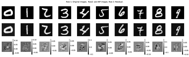
Figure 1: Samples from MNIST - one per class, before (top row) and after (middle row) optimization with adv-KIP. The bottom row shows the residual between the images of that column. Performance of NTK kernel regression on original data: 98.46% clean test accuracy, 0.07% robust test accuracy. On optimized data: 97.67% clean test accuracy, 42.94% robust test accuracy. adv-KIP hyperparameters: $\epsilon=0.3$, 10 PGD steps, $\alpha=0.1$, fully connected ReLU NTK with 3 layers, dataset size is 40,000.

In this work, we initiate such a data-based approach to robustness in a principled way. We propose a gradient-based approach for solving the optimization problem in Eq. (2), adopting kernel regression; focusing on a particular class of kernel functions, Neural Tangent Kernels (NTKs). Kernel regression with NTKs is known to describe the training process of infinitely wide networks (Jacot et al., 2018; Lee et al., 2019; Arora et al., 2019), providing a natural choice for the optimization of datasets for eventual deployment in neural networks. Prior work on dataset distillation (the process of distilling information from one dataset to a smaller, optimized, one) has found that meta-optimization using NTKs produces highly transferable datasets suitable for neural network training (Nguyen et al., 2021a, b). Their algorithm, Kernel Inducing Point (KIP), serves as an inspiration for this work; thus we give the name adv-KIP to our novel meta-learning algorithm for iteratively solving Eq. (2).

We perform a wide range of experiments on standard image recognition datasets (MNIST and CIFAR-10) using adv-KIP with a variety of different kernels and perturbation sets $\Delta$, and discuss important design choices (dataset size, meta-optimizer, loss choices etc). We establish that the meta-learning algorithm converges to training datasets which look similar to the original ones (see Fig. 1), when used as a training set guarantee similar performance on an (unperturbed) test set, but additionally, and importantly, are also able to produce models capable of defending against gradient-based attacks.

However, we find that the models struggle to withstand non-gradient based, or adaptive, attacks. Interestingly, we observe that both neural networks and kernels that are trained on our optimized datasets have vanishing gradients with respect to the input, thus causing gradient based attacks to fail. This phenomenon, known in the literature under the umbrella term of obfuscated gradient (Athalye et al., 2018), has been observed in the past, but has been largely connected to (failed) defensive interventions on models and architectures (stochastic/discrete layers etc. ). Our findings show that it can also be observed in more “benign” settings, and can also be a property of the data alone.

Armed with these insights, we revisit seminal work of Ilyas et al. (2019) that put forward a dichotomy between robust and non-robust features (Tsipras et al., 2019; Allen-Zhu & Li, 2022; Tsilivis & Kempe, 2022) in the data. To bolster their argument, Ilyas et al. (2019) construct a dataset (using an already adversarially trained model) thought to contain solely robust features and demonstrate that a freshly initialized neural network (standardly) trained on this dataset is able to achieve non-trivial performance against gradient based attacks. Remarkably, upon re-examination, we find that models trained with these optimized datasets also suffer from the vanishing gradient problem and fail to withstand adaptive attacks, thus shattering a long standing claim in the community. Collectively, our findings establish that adversarial robustness from data alone is far more challenging than previously thought. We believe that our insights will help design and faster debug other data-based approaches in the future.

In summary, our contributions are two-fold:

• We devise a principled data based meta-learning algorithm, adv-KIP, tackling the bi-level optimization for adversarially robust classification in a novel way, with potentially wider applicability. We perform experiments on standard computer vision benchmarks and analyze the properties of models (kernels and neural networks) fit on the optimized datasets demonstrating that they enjoy remarkable robustness against gradient-based attacks.

• We show that robustness from data alone is more challenging than previously assumed. Standard models trained with gradient descent on datasets from adv-KIP suffer from the “obfuscated gradient” phenomenon, without explicitly adding non-smooth elements to the computational pipeline. We find that this is also the case for models trained with datasets presumably containing solely robust features (Ilyas et al., 2019). That is, all these models fail to withstand non-gradient based adversarial attacks, once the size of the perturbation is large enough. We examine and discuss the properties of all the models, in terms of confidence and calibration and draw lessons for future dataset design.

2 Preliminaries

Adversarial Training. Eq. 1 establishes the min-max underpinning for the construction of adversarially robust classifiers (Madry et al., 2018). The most common way to approximate the solution of this optimization problem for a neural network $f$ is to first generate adversarial examples by running multiple steps of projected gradient descent (PGD) (Kurakin et al., 2017; Madry et al., 2018). When the set of allowed perturbations $\Delta$ is ${\mathcal{B}_{\mathbf{x}}^{\epsilon}}$ - the $\ell_{\infty}$ ball of radius $\epsilon$ and center $\mathbf{x}$ - the iterative $N$-step approximation is given by

$$\mathbf{x}^{k+1}=\Pi_{\mathcal{B}_{\mathbf{x}^{0}}^{\epsilon}}\left(\mathbf{x}^{k}+\alpha\cdot\mathrm{sign}(\nabla_{\mathbf{x}^{k}}\mathcal{L}(f(\mathbf{x}^{k}),y)\right),$$ (3)

where $\mathbf{x}^{0}=\mathbf{x}$ is the original example, $\alpha$ is a learning step, $\tilde{\mathbf{x}}=\mathbf{x}^{N}$ is the final adversarial example, and $\Pi$ is the projection on the valid constraint set of the data. During adversarial training we alternate steps of generating adversarial examples (using $f$ from the current network) and training on this data instead of the original one. Several variations of this approach have been proposed in the literature (e.g. (Zhang et al., 2019; Shafahi et al., 2019; Wong et al., 2020b)), modifying either the attack used for data generation (inner loop in Eq. (1)) or the loss in the outer loop.

Kernel Regression, NTK and KIP. Kernel regression is a fundamental non-linear regression method. Given a dataset $(\mathcal{X},\mathcal{Y})$ , where $\mathcal{X}\in\mathbb{R}^{n\times d}$ and $\mathcal{Y}\in\mathbb{R}^{n\times k}$ (e.g., a set of one-hot vectors), kernel regression computes an estimate

$$\hat{f}(\mathbf{x})=K(\mathbf{x},\mathcal{X})^{\top}K(\mathcal{X},\mathcal{X})^{-1}\mathcal{Y},$$ (4)

where $K(\mathbf{x},\mathcal{X})=[k(\mathbf{x},\mathbf{x}_{1}),\ldots,k(\mathbf{x},\mathbf{x}_{n})]^{\top}\in\mathbb{R}^{n}$, $K(\mathcal{X},\mathcal{X})_{ij}=k(\mathbf{x}_{i},\mathbf{x}_{j})$ and $k$ is a kernel function that measures similarity between points in $\mathbb{R}^{d}$.

Recent work in deep learning theory has established a profound connection between kernel regression and the infinite width, low learning rate limit of deep neural networks (Jacot et al., 2018; Lee et al., 2019; Arora et al., 2019). In particular, it can be shown that the evolution of such suitably initialized infinitely wide neural networks admits a closed form solution as in Eq. (4), with a network-dependent kernel function $k$. Focusing on a scalar neural net $f$ for ease of notation, it is given by:

$$k(\mathbf{x}_{i},\mathbf{x}_{j})=\nabla_{\theta}f(\mathbf{x}_{i};\theta)^{\top}\nabla_{\theta}f(\mathbf{x}_{j};\theta),$$ (5)

where $\theta$ are the parameters of the network. This expression becomes constant (in time) in the infinite width limit.

Many fruitful applications of NTK theory to machine learning practice have already benefited from the equivalence between kernels and neural networks (Tancik et al., 2020; Chen et al., 2021; Nguyen et al., 2021b). Our work builds on a recently proposed dataset distillation (Wang et al., 2018a) algorithm called Kernel Inducing Points (KIP) (Nguyen et al., 2021a, b). These works introduce a meta-learning algorithm for data distillation from an original training set $\mathcal{D}$, to an optimized source set $(\mathcal{X}_{S},\mathcal{Y}_{S})$ of reduced size but of similar generalization properties. The closed form of Eq. (4) allows to express this objective via a loss function on a target data set $(\mathcal{X}_{T},\mathcal{Y}_{T})$ as:

$$\mathcal{L}_{\mathrm{KIP}}(\mathcal{X}_{S},\mathcal{Y}_{S})=\|\mathcal{Y}_{T}-K(\mathcal{X}_{T},\mathcal{X}_{S})^{\top}K(\mathcal{X}_{S},\mathcal{X}_{S})^{-1}\mathcal{Y}_{S}\|_{2}.$$ (6)

The error of Eq. (6) can be minimized via gradient descent on $\mathcal{X}_{S}$ (and optionally $\mathcal{Y}_{S}$). Starting with a smaller subset of $\mathcal{D}$, sampling a target dataset from $\mathcal{D}$ to simulate test points, and backpropagating the gradients of the error with respect to the data allows to progressively find better and better synthetic data. Importantly, leveraging the NTK for kernel regression renders the datasets suitable for deployment on actual neural nets as well.

Prior work on dataset optimization. To the best of our knowledge, the idea of trying to obtain robust classifiers through data or representation optimization is rather unexplored. Garg et al. (2018) design a spectral method to extract robust embeddings from a dataset. Awasthi et al. (2021) formulate an adversarially robust formulation of PCA, to extract provably robust representations. Ilyas et al. (2019) construct a robust dataset by traversing the representation layer of a previously trained robust classifier, which presumably contains solely robust features. Yet, all of these methods achieve substantially lower robust accuracy compared to adversarial training.

3 adv-KIP Algorithm

In this section, we introduce our meta-learning approach, adv-KIP, for adversarially robust classification. It optimizes a dataset prior to its deployment so that a model fit on it will have predictions that are robust against worst case perturbations of a testing input. That is, our algorithm inputs a dataset, outputs a dataset and carries out optimization (i.e. gradient updates) on the data level. Similarly to the KIP method (Nguyen et al., 2021a, b) outlined in Section 2, our method works with kernel machines, and especially with NTKs. However, the goal here is slightly different from the KIP objective; instead of deriving a dataset of reduced size, we aim to create one that induces better robustness properties on the original unmodified test set. For further connections with previous work in adversarially robust classification, see App. A.1.

We modify the meta-objective of Eq. (6), and instead of optimizing the data $(\mathcal{X}_{S},\mathcal{Y}_{S})$ with respect to the “clean” loss of Eq. (6), we minimize

$$\tilde{\mathcal{L}}(\mathcal{X}_{S},\mathcal{Y}_{S})=\|\mathcal{Y}_{T}-K(\tilde{\mathcal{X}}_{T},\mathcal{X}_{S})^{\top}K(\mathcal{X}_{S},\mathcal{X}_{S})^{-1}\mathcal{Y}_{S}\|_{2},$$ (7)

where, in a slight abuse of notation, $\tilde{\mathcal{X}}_{T}=\mathcal{X}_{T}+\tilde{\delta}$, and

$$\tilde{\delta}=\arg\max_{\delta\in\Delta}\mathcal{L}(K(\tilde{\mathcal{X}}_{T},\mathcal{X}_{S})^{\top}K(\mathcal{X}_{S},\mathcal{X}_{S})^{-1}\mathcal{Y}_{S},\mathcal{Y}_{T}).$$ (8)

In other words, we optimize the data $(\mathcal{X}_{S},\mathcal{Y}_{S})$ to achieve the best possible performance of kernel regression on the target data set after the adversarial attack. Notice that this approach solves the problem outlined in Eq. (2), by adding an inner maximization problem to the KIP framework. Solving this optimization now requires an inner loop that tackles the maximization in Eq. (8). As is common, we employ first order gradient methods to solve this, namely projected gradient ascent (on the loss of the kernel machine). Algorithm 1 describes our generic robust training data set distillation framework for the case of an $\ell_{\infty}$ threat model, though it is easily modified to any constraint set $\Delta$.

Input: A training dataset $\mathcal{D}_{\mathrm{train}}=\{\mathcal{X},\mathcal{Y}\}$.

Parameters : Number of (meta) $\mathrm{epochs}$, number of $\mathrm{pgd\_steps}$, pgd step size $\alpha$, max attack size $\epsilon$, (meta) learning rate $\lambda$.

Output: A new dataset $\mathcal{D}_{\mathrm{rob}}$.

1 Sample data $\mathcal{S}=\{\mathcal{X}_{S},\mathcal{Y}_{S}\}$ from $\mathcal{D}_{\mathrm{train}}$;

2 for $\mathrm{i}\leftarrow 1$ to $\mathrm{epochs}$ do

3       Sample data $\mathcal{T}=\{\mathcal{X}_{T},\mathcal{Y}_{T}\}$ from $\mathcal{D}_{\mathrm{train}}$;

4       for $\mathrm{j}\leftarrow 1$ to $\mathrm{pgd\_steps}$ do

5             $\mathcal{X}_{T}\leftarrow\mathcal{X}_{T}+\alpha\cdot\mathrm{sign}(\nabla_{\mathcal{X}_{T}}\mathcal{L}_{\mathrm{ce}}(K_{\mathcal{X}_{T}\mathcal{X}_{S}}K_{\mathcal{X}_{S}\mathcal{X}_{S}}^{-1}\mathcal{Y}_{S},\mathcal{Y}_{T}))$;

6             $\mathcal{X}_{T}\leftarrow\Pi_{\mathcal{B}_{\epsilon}}(\mathcal{X}_{T})$;

7            

8      $\mathcal{X}_{S}\leftarrow\mathcal{X}_{S}-\lambda\nabla_{\mathcal{X}_{S}}\mathcal{L}(K_{\mathcal{X}_{T}\mathcal{X}_{S}}K_{\mathcal{X}_{S}\mathcal{X}_{S}}^{-1}\mathcal{Y}_{S},\mathcal{Y}_{T})$;

9       $\mathcal{Y}_{S}\leftarrow\mathcal{Y}_{S}-\lambda\nabla_{\mathcal{Y}_{S}}\mathcal{L}(K_{\mathcal{X}_{T}\mathcal{X}_{S}}K_{\mathcal{X}_{S}\mathcal{X}_{S}}^{-1}\mathcal{Y}_{S},\mathcal{Y}_{T})$;

10      

$\mathcal{D}_{\mathrm{rob}}\leftarrow(\mathcal{X}_{S},\mathcal{Y}_{S})$

Algorithm 1 adv-KIP for $\ell_{\infty}$ adversarial attacks

Algorithmic choices / Hyperparameters: There are several options to specialize in Algorithm 1:

Outer loss function (lines 7 and 8): This can be either the mean squared error (as in Eq. (7)) or the more flexible cross entropy loss. Both quantify the discrepancy between the prediction of the kernel machine on the perturbed data and the ground truth labels. Alternatively, a loss that balances clean and robust accuracy (see e.g. (Zhang et al., 2019)) can be used.

Inner loss function (line 5): Instead of using the cross entropy loss for the generation of adversarial examples, we can also adopt previously proposed methods, like the CW-loss (Carlini & Wagner, 2017).

Optimization of labels (line 8): This is related to an interesting question raised in prior work: How important are rigid one-hot labels for robust classification (see e.g. (Papernot et al., 2016) for an ultimately unsuccessful defense). Algorithm 1 as presented here optimizes the labels, by backpropagating the loss gradients. It has the flexibility, however, to omit this part (by omitting line 8).

Dataset Size $|\mathcal{X}_{S}|$: While the goal of the algorithm is to ultimately produce a robust dataset, a reduced dataset size could be a useful by-product, by initializing with $|\mathcal{X}_{S}|<|\mathcal{X}|$ samples.

Meta-Optimizer (lines 7 and 8): Algorithm 1 presents the simplest possible version of adv-KIP; but the (meta) optimization of the data $\{\mathcal{X}_{S},\mathcal{Y}_{S}\}$ can also be implemented with other algorithms, such as adaptive gradient methods. Indeed, in the experiments, following the code implementation of KIP (Nguyen et al., 2021a), we adopt the Adam optimizer (Kingma & Ba, 2015) instead of gradient descent.

Algorithmic Framework for Broader Data-Based Problems: Algorithm 1 is an approach to a particular min-max problem given in Eq. (2). The advantage of deploying the NTK here is that it affords an analytic surrogate expression for the output of the trained neural networks, which allows to compute gradients with respect to the input dataset. We expect that our framework can be adopted and be helpful in other problems in data-centric machine learning, such as, for instance, average case robustness (Hendrycks & Dietterich, 2019), discrimination against minority groups (Hashimoto et al., 2018), few-shot learning (where the inner loop would optimize for accuracy on a small out-of-distribution target set) and possibly others.

4 Experiments

We evaluate the performance of adv-KIP on standard computer vision benchmarks. Specifically, we perform experiments on MNIST (Deng, 2012) and CIFAR-10 (Krizhevsky, 2009) against $\ell_{\infty}$ and $\ell_{2}$ adversaries. In all cases, robust performance is measured on the original test dataset. We experiment with kernels that correspond to fully connected and convolutional architectures of relatively small depth, due to the high computational cost of evaluating the NTK expressions. All our experiments are based on expressions available through the Neural Tangents library (Novak et al., 2020), built on top of JAX (Bradbury et al., 2018). Adversarial attacks are implemented using the CleverHans library (Papernot et al., 2018) (or slightly modified versions for efficient deployment on kernels). FCd and Convd denote the NTK of a $d$-layer infinitely wide fully-connected ReLU neural network and (fully) convolutional ReLU neural network with an additional fully connected last layer, respectively.

4.1 Meta-Learning and Kernel results

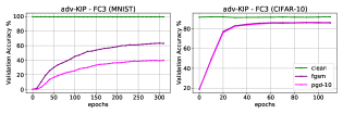
Figure 2: Validation accuracies during meta-optimization with adv-KIP. Setting: FC3 kernel, $|\mathcal{X}_{S}|=40K$, $|\mathcal{X}_{T}|=10K$, $\ell_{\infty}$ adversary, (left) MNIST $\epsilon=0.3$, $\alpha=0.1$, 10 PGD steps, (right) CIFAR-10 $\epsilon=8/255$, $\alpha=2/255$, 10 PGD steps.

We implement Algorithm 1 with the Adam optimizer (with fixed learning rate equal to $1e$-3) for a few hundred epochs with multi-step PGD attacks, using standard values of perturbation budget $\epsilon,\alpha$. The datasets are initialized as balanced, i.e. they contain the same number of samples from each class. The performance of the algorithm is evaluated every few epochs on a hold out validation set (part of the original training dataset), and we terminate if validation robust accuracy ceases to increase.

For both MNIST and CIFAR-10, we observe that adv-KIP is able to converge in a few epochs of meta-training (see Fig. 2). Validation accuracy against FGSM and PGD attacks increases with the number of outer loop steps, essentially without compromising performance on clean data. Note that at the start of the optimization (corresponding to the original data) the robustness of the kernel machine is very low, as expected from studies on neural nets.

Table 1 summarizes the test results on kernel machines. All kernel classifiers are fit with the adv-KIP-produced dataset meta-optimized with the same kernel. We see that just 5,000 images on MNIST suffice to yield a Conv3 classifier scoring $96.31\%$ test accuracy and $76.62\%$ robust test accuracy (evaluated against strong PGD attacks of same strength as used in the inner-loop optimization with radius $\epsilon=0.3$). Notice that all the robust benefit comes from the new, optimized images (no change in the model). We also note that the convolutional kernel achieves better performance, despite the fact that we deploy it with a much smaller dataset $\mathcal{X}_{S}$ of size $5,000$. This indicates that convolutional architectures might be more amenable to meta-optimization than their fully connected counterparts. On CIFAR-10, we see a marked drop in both clean and robust accuracy; note, however, that fully connected kernels are not very competitive classifiers for CIFAR-10 images. To achieve some level of robustness with these simple architectures gives credence to our approach. To the best of our knowledge, this is a first (empirical) demonstration of some robustness of simple machine learning models, such as kernel methods, to adversarial attacks.

As an ablation study, we measure robust accuracy on datasets produced by the original KIP algorithm (Nguyen et al., 2021a, b) which is designed for reduction of dataset size, while keeping (clean) accuracy as uncompromised as possible. It could be reasonable to hypothesize that such information compression might possibly lead to an increase of robustness as well, but we find that this is not at all the case. We also experimented with larger KIP datasets of the same cardinality as the ones of Table 1. In all cases, we find that KIP datasets do not provide any robust accuracy, neither against FGSM nor PGD attacks (see Appendix A.2 for more details). This indicates the clear need to adjust the optimization objective to robust performance, as is done in the adv-KIP algorithm.

Table 1: Test accuracy $\%$ (clean and robust) of kernel machines using the optimized adv-KIP datasets. For MNIST ($\ell_{\infty}$): $\epsilon=0.3$, $\alpha=0.1$, $10$ PGD steps. For CIFAR-10 ($\ell_{\infty}$): $\epsilon=8/255$, $\alpha=2/255$, $6$ PGD steps. For CIFAR-10 ($\ell_{2}$): $\epsilon=1.$, $\alpha=0.2$, $10$ PGD steps. These exact same hyperparameters are used for attacks in the inner loop of the dataset meta-optimization.

			Robust
Dataset	Kernel, $|\mathcal{X}_{s}|$	Clean	FGSM	PGD
MNIST ($\ell_{\infty}$)	Conv3, 5k	96.31	94.82	76.62
	FC7, 30k	97.21	67.04	50.34
CIFAR-10 ($\ell_{\infty}$)	FC2, 40k	59.65	20.49	20.37
	FC3, 40k	60.14	36.44	36.30
CIFAR-10 ($\ell_{2}$)	FC3, 40k	59.84	29.90	29.63

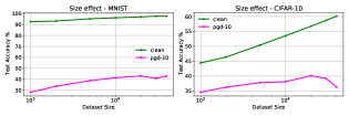
Figure 3: Performance of adv-KIP outputs as a function of dataset size. Setting: FC3 kernel, $|\mathcal{X}_{T}|=10k$, $\ell_{\infty}$ adversary, $\epsilon=0.3$ ($\epsilon=8/255$), $\alpha=0.1$ ($\alpha=2/255$).

We also examine the importance of scale on the final robustness of the dataset. We run adv-KIP on MNIST and CIFAR-10, using an FC3 kernel for a wide variety of different dataset sizes $|\mathcal{X}_{S}|$, while keeping the rest of the hyperparameters the same. We optimize for 500 meta epochs and use early stopping if robust validation accuracy ceases to improve. For all the runs, we observe that we stop early, so we conclude that all the datasets were given a fair chance. On the test set we then evaluate the same kernel classifier fit with the optimized data, recording clean and robust accuracy. The scaling laws are shown in Fig 3. We observe diminishing returns on the performance of the models, after we exceed some required sample size. For the more challenging setting (CIFAR-10) it is the clean accuracy that sees the greater increase. The fact that the robust curve “bends” in the end might mean that we could optimize more agressively by harming clean accuracy (without implementing early stopping).

4.2 Neural Networks results

In this section, we study whether datasets produced with adv-KIP can be used to train robust neural networks.

Wide fully connected neural networks. As a first step, we perform experiments on the same architecture as in the NTK used in the meta-optimization of the dataset. We consider fully connected ReLU models with 2, 3, 5 and 7 layers of width $1024$ and train them using Adam. We refer to App. A.3 and A.4 for full experimental details and results. We find that in all cases the networks learn successfully with clean and robust test performance that matches or exceeds those of the kernels (even when evaluating against stronger attacks with more PGD steps than used during the meta-optimization). We view this is an indication that features learned by kernels are surprisingly relevant for (robust) classification in neural networks.

Robustness of Common Architectures. We now turn our attention to commonly employed convolutional neural networks to study the relevance of our datasets for robust classification using modern architectures. In particular we report how datasets generated using FC kernels transfer to such convolutional architectures, since the small datasets generated from Conv kernels were challenging to fit with neural networks. We consider a simple CNN with 3 convolutional layers with max-pooling operations on MNIST, and AlexNet (Krizhevsky et al., 2012), VGG11 (Simonyan & Zisserman, 2015) and ResNet20 (He et al., 2016) on CIFAR-10. We perform a sweep over different learning rates and training algorithms (gradient descent, gradient descent with weight decay and Adam). Experimental details can be found in App. A.3.

Tables 2 and 3 summarize our findings. We note an astonishing “boost” in robust test accuracy against gradient-based attacks of these convolutional networks (in all models but ResNet) when compared to the previous results on kernels and fully connected networks. Very remarkably, it seems that datasets optimized for relatively simple kernels “transfer” their PGD-performance to networks far removed from the idealistic infinite width regime, even to more expressive architectures. We also note that the results are robust to the initialization of the networks, as evidenced by the deviations reported in the tables.

Table 2: MNIST with simple-CNN: Test accuracies when trained on adv-KIP datasets optimized with FC kernels (first 3 rows). We also show test accuracies for the adversarially trained simple-CNN (without any data augmentation). AA refers to the AutoAttack test suite. Setting: $\ell_{\infty}$, $\epsilon=0.3,\alpha=0.1$.

		Robust
Dataset	Clean	FGSM	PGD40	AA
FC3	98.15 $\pm$ 0.12	98.06 $\pm$ 0.18	97.17 $\pm$ 0.10	0.00 $\pm$ 0.00
FC5	97.96 $\pm$ 0.55	97.87 $\pm$ 0.64	97.20 $\pm$ 0.74	0.00 $\pm$ 0.00
FC7	98.03 $\pm$ 0.16	97.91 $\pm$ 0.22	97.14 $\pm$ 0.43	0.00 $\pm$ 0.00
Adversarial Training	99.11	97.52	95.82	88.77

Table 3: CIFAR-10: Test accuracies of several convolutional architectures trained on an adv-KIP dataset produced from an FC3 kernel of $|\mathcal{X}_{S}|=40,000$ (upper), and Adversarial Training baselines (lower). Setting: $\ell_{\infty}$, $\epsilon=8/255,\alpha=2/255$. For further results on smaller attack radii, see Table 8 in App. A.5.

adv-KIP
Neural Net	Clean	FGSM	PGD20	AA
Simple CNN	72.10 $\pm$ 0.10	67.45 $\pm$ 0.37	67.03 $\pm$ 0.24	0.00 $\pm$ 0.00
AlexNet	68.87 $\pm$ 0.76	49.30 $\pm$ 0.69	49.06 $\pm$ 0.63	0.89 $\pm$ 1.41
VGG11	74.88 $\pm$ 0.45	53.98 $\pm$ 9.71	53.18 $\pm$ 10.32	0.27 $\pm$ 0.18
ResNet20	81.53 $\pm$ 0.59	4.82 $\pm$ 1.45	0.20 $\pm$ 0.16	0.00 $\pm$ 0.00
Adversarial Training Baseline
Neural Net	Clean	FGSM	PGD20	AA
Simple CNN	58.07	33.94	31.49	26.18
AlexNet	44.35	30.12	24.41	18.95
VGG11	69.69	31.41	24.88	24.09
ResNet20	73.95	46.37	39.17	35.35

Fig. 4 (top left) shows accuracy curves for the CNN when trained on the optimized CIFAR-10 dataset. While accuracy on the train (optimized) data together with the clean test accuracy increase rapidly, it is only after 250 epochs that robust accuracy starts to increase (after we hit 0 training loss). We hypothesize that this might be due to the fact that adv-KIP optimizes using the expression that corresponds to the end of training in neural networks.

It seems promising at first that modern networks trained with adv-KIP datasets without much tuning enjoy astonishing defense properties against PGD-attacks in various settings, similar, or in some cases even higher, than what truly robust models (i.e adversarially trained) obtain. However, as can be seen in the last column of Tables 2 and 3, when we evaluate their robustness with the adaptive methods of AutoAttack (Croce & Hein, 2020), we observe a sharp drop in the performance (close to 0% in all cases). The purpose of the AutoAttack benchmark, which includes 4 different attacks, some of which do not use gradient information, is to provide a minimal adaptive attack suite to uncover shortcomings in a defense. See Table 9 in App. A.6 for a breakdown of robustness by AutoAttack components.

We find that datasets produced with adv-KIP suffer from what is commonly termed the obfuscated gradient phenomenon (Athalye et al., 2018), a situation where model gradients do not provide good directions for generating successful adversarial examples. However, in the past, this has only been observed with techniques that were either introducing non-differentiable parts in the inference pipeline or stochasticity to the model. Interestingly, we now observe this phenomenon from altering the training data alone and, even more remarkably, from data optimized using kernels.

To check whether this is a shortcoming of our optimization method or a more general phenomenon related to ”robustified” datasets, we turn our attention next to the only other method we are aware of that provides some notable robustness via standard training (Ilyas et al., 2019).

4.3 Non-robustness of Robust Features dataset

To illustrate the theory of the presence of robust and non-robust features in the data, Ilyas et al. (2019) have introduced a “robustified” data set (termed Robust Features Dataset or RFD from now on), which was sufficient to ensure robust predictions on the test set by standard training only. RFD is generated by traversing the representation layer of an adversarially trained neural network, and was thus believed to provide a general sense of robustness (Ilyas et al., 2019). More specifically, given a mapping $x\mapsto g(x)$ of an input $x$ to the penultimate (“representation”) layer of an adversarially trained neural net, a “robustified” input is obtained by optimizing $\min_{x_{r}}\|g(x)-g(x_{r})\|_{2}$, starting from a random data point using gradient descent, thus enforcing that the robust representations of $x$ and $x_{r}$ are similar; while $x_{r}$ does not contain non-robust features given a starting point that is uncorrelated with the label of $x$.

We use an $\ell_{\infty}$-adversarially trained ResNet50 to generate an RFD version of CIFAR-10. To ensure a fair comparison with our methods, we train the same set of models as in the previous subsection. Table 4 contains the results.

Table 4: Test accuracies for various models trained on a 50K $\ell_{\infty}$ Robust Features dataset (Ilyas et al., 2019)) for CIFAR-10. Setting: $\ell_{\infty}$, $\epsilon=8/255,\alpha=2/255$. For further results on smaller attack radius, see Table 7 in App. A.5.

Robust Features dataset (Ilyas et al., 2019)
Neural Net	Clean	PGD20	AA
Simple CNN	59.15 $\pm$ 0.37	52.91 $\pm$ 0.66	0.00 $\pm$ 0.00
AlexNet	51.62 $\pm$ 1.14	25.64 $\pm$ 4.32	0.02 $\pm$ 0.03
VGG11	61.59 $\pm$ 0.80	34.64 $\pm$ 8.47	0.40 $\pm$ 0.42
ResNet20	66.29 $\pm$ 0.70	7.35 $\pm$ 3.10	0.00 $\pm$ 0.00

Confirming the findings of Ilyas et al. (2019), we see that the trained models record high robustness against PGD attacks. However, all of the models fail to defend against AutoAttack. This is a surprising finding, since the dataset was generated using adversarially trained networks that guarantee a wide sense of robustness (Croce et al., 2020). In Fig. 4 (middle), we can see that the simple CNN when trained on the RFD exhibits remarkably similar accuracy curves as when being trained on an adv-KIP dataset. In the next subsection, we dive deeper into the similarities between the two classes of datasets.

4.4 Overconfidence gives a false sense of security

Figure 4: Several statistics of CNN models trained on an adv-KIP dataset (first row), an RFD (second row), and trained with adversarial training (third row). From Left to Right: Accuracy, Test Loss (decomposed in correctly and wrongly classified examples); Average Gradient Norm of Test data; Confidence Histogram. Base dataset: CIFAR-10.

We analyze properties of models that were trained with either an adv-KIP or an RF dataset and yield superficial robustness. We discover many common properties and signatures of failure, and contrast them to adversarially trained neural networks. These similarities might be germane to all attempts that explicitly optimize the dataset with gradient based approaches.

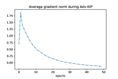
Figure 6: The average gradient norm of an FC3 kernel on a validation set during the distillation procedure of Algorithm 1. We see that the training data evolves to cause gradient shrinkage of the model. Setting: CIFAR-10, FC3, $|\mathcal{X}_{S}|$ = 40k, $|\mathcal{X}_{T}|$ = 10k, 10 PGD steps, cross entropy loss in outer loop.

Fig. 4 (second and third column) shows the loss value and the gradient magnitude of the models throughout training, where we further decomposed the metrics into 2 parts; one coming from correctly classified images and one from misclassified ones. We observe that for both datasets the loss increases on the misclassified examples, concurrently with an increase of the average norm of the gradient. In contrast, for correctly classified examples we see both quantities progressively vanish. This behavior, together with the false sense of robustness that AutoAttack evaluation reveals, suggests that the model learns to shatter the gradients locally in the neighborhood of correctly classified examples, causing simple gradient-based attacks to fail. We find that during our distillation procedure this is indeed the case (Fig. 6 in the Appendix), and the data optimization effectively shrinks the gradients of the model.

In other words, the model essentially “sacrifices” performance on the subset of data that is misclassified, in order to fit the rest in a pseudo robust way. This is in sharp contrast with the situation during adversarial training, where the loss decreases on all data simultaneously (Fig. 4, third row). This is already an indication of failure of learning. Interestingly, Fig. 4 (third column) shows that this failure of learning is also evident in the gradient norms of the loss with respect to the input. The average gradient norm on the wrongly classified points explodes with the number of epochs for both the adv-KIP dataset and the RFD.

Finally, we study the calibration of the models. In particular, we compute confidence histograms and reliability diagrams (Guo et al., 2017) for the 3 models. As Fig. 4 (last column) shows, the models that were trained with the adv-KIP dataset or the RFD are extremely confident on nearly all test examples, being poorly calibrated, while the adversarially trained model has a completely different, more balanced, profile (it is less confident than accurate). We refer to Fig. 5 in App. A.8 for the reliability diagram of the 3 models that provides further evidence for the above. In a sense, this overconfidence on the samples is what makes the gradients non-informative.

Understanding why the solution of Eq. (2) (data level) with gradient based methods gives a false sense of robustness, while the solution of Eq. (1) (parameters level) also with gradient based methods induces more widespread robustness seems a very interesting and challenging open question for future work to address.

5 Conclusion

In this work, we approached the problem of robust classification in machine learning from a data-based point of view. We introduced a meta-learning algorithm, adv-KIP, which produces datasets that furnish a great range of classifiers with notable robustness against gradient-based attacks. However, our analysis demonstrates that this robustness is rather fallacious and the models essentially learn representations that provide no meaningful gradients. Quite remarkably, when we revisited seminal prior work (Ilyas et al., 2019) that claimed standard training on a robust dataset can be an actual defense versus adversarial attacks, we found the same pathological situation. We believe our findings provide many new insights on the role of data in adversarially robust classification and should be helpful for potential new data-based approaches in the future.

Appendix A Appendix

A.1 Related Work

Distributionally Robust Optimization and Adversarial Augmentation. Related to our work are also works on distributionally robust optimization (Sinha et al., 2018) and adversarial data augmentation for out-of-distribution generalization (Volpi et al., 2018). The latter proposes an algorithm that augments the training dataset on-the-fly (i.e. during training of a neural net) with worst-case samples from a target distribution. In contrast, our method optimizes the original dataset against worst-case samples/adversarial examples from the original distribution, which correspond to a final predictor (kernel machine). The only prior work that gives an algorithm based on NTK theory to derive dataset perturbations in some adversarial setting is due to Yuan & Wu (2021), yet with entirely different focus. It deals with what is coined generalization attacks: the process of altering the training data distribution to prevent models to generalise on clean data. To our knowledge, KIP (Nguyen et al., 2021a, b) and this NTGA algorithm are the only examples of leveraging NTKs for dataset optimization.

A.2 KIP baseline

The original KIP algorithm (Nguyen et al., 2021a, b) is designed to reduce the size of the training set, while keeping the induced accuracy close to the original one. It could be reasonable to hypothesize that such information compression might possibly lead to an increase of robustness as well. As a sanity check we evaluate the robust accuracy of these datasets. We also produce larger dataset using the KIP algorithm (of the same size as used in our adv-KIP experiments). Table 5 shows that effectively the robustness of the datasets remains close to 0, as is the case for the original datasets. This indicates the clear need to adjust the optimization objective to robust performance, as is done in the adv-KIP algorithm.

Table 5: KIP baseline datasets (reproduced). Setting: No preprocessing/data augmentation, $|\mathcal{X}_{T}|=$1,000 images, learned labels, mse loss, lr=$1$e-3, datasets were optimized for 1000 epochs, with potential early stopping if validation accuracy did not increase across 200 epochs. Random seed denotes different draws of the initial support images. Standard setting for robust evaluation: $\epsilon=0.3$ and $\epsilon=8/255$, respectively.

	Kernel, $|\mathcal{X}_{s}|$	Clean	FGSM
MNIST	FC3, 5k	97.51 $\pm$ 0.03	0.00 $\pm$ 0.00
	FC7, 30k	98.23 $\pm$ 0.06	0.00 $\pm$ 0.00
CIFAR-10	FC3, 1k	48.45 $\pm$ 0.34	2.50 $\pm$ 0.21
	FC3, 5k	52.48 $\pm$ 0.23	0.22 $\pm$ 0.05
	FC3, 10k	54.04 $\pm$ 0.41	0.10 $\pm$ 0.04

We also evaluated FC$\{3,5,7\}$ and Conv$\{3,5,7\}$ kernels (together with a Convolutional Kernel with 1 hidden layer followed by global average-pooling) on datasets (with 50 images per class) released by (Nguyen et al., 2021b) and we found their FGSM robustness to be 0$\%$ in all cases. URLs for the datasets we considered: 1st and 2nd.

A.3 Experimental Details for Neural Network experiments

For all models trained on an adv-KIP dataset or an RFD, we use the Adam optimizer and perform a small grid search for the learning rate, picking the best model with respect to robust accuracy.

On MNIST, we train fully connected networks of width 1024 in Sec. A.4, and the simple-CNN network in Sec. 4. FC networks are trained for 2,000 epochs and the simple-CNN network for 800 epochs.

On CIFAR-10, we again train fully connected networks of width 1024 in Sec. A.4, and the simple-CNN, AlexNet and VGG11 networks in Sec. 4. We train all these networks for 2,000 epochs.

For the Adversarial Training baseline, on MNIST, we adopt the setting of (Madry et al., 2018), that is we train the simple-CNN network with the Adam optimizer towards convergence, and set the initial learning rate to 1e-4. In (Madry et al., 2018) the number of epochs was set to 100, while we use 200. On CIFAR-10, since we do not use data augmentation, we train with both SGD and Adam for 200 epochs for each model, and pick the better one in terms of robustness. For the simple-CNN and AlexNet, the Adam optimizer is better. For VGG11, we use the SGD optimizer, with initial learning rate 1e-1, decay rate of 10 at the 100-th and the 150-th epoch, and with weight decay 5e-4.

Simple-CNN architecture: We use a simple convolutional architecture with three convolutional layers and a linear layer. Each convolutional layer computes a convolution with a 3$\times$3 kernel, followed by a ReLU and a max-pooling layer (of kernel size 2$\times$2 and stride 2). The linear layer is fully-connected with ten outputs. All convolutional layers have a fixed width of 64.

Training of Convolutional Nets: We use the Adam optimizer (Kingma & Ba, 2015) and perform a small grid search over the fixed learning rate. We stop training when robust validation accuracy ceases to decrease, where we measure against PGD40 attacks for MNIST and PGD20 attacks for CIFAR-10, as is often standard. We report the best results across the sweep for FGSM and PGD test accuracies. After picking the best learning rate, for each experiment in this paper, we report the mean and standard deviation of three experiments with different seeds.

Description of Evaluation Metrics: For all the adversarial attack related measurements including FGSM, $\ell_{\infty}$ PGD and $\ell_{2}$ PGD, we adopt the CleverHans code implementation (Papernot et al., 2018). For $\ell_{\infty}$ PGD, on MNIST we use step size 0.1 and radius 0.3, while on CIFAR-10 we use step size 2/255 and radius 8/255. For $\ell_{2}$ PGD on CIFAR-10, we use step size 15/255 and radius 128/255.

For AutoAttack, we adopt the open-source original implementation (Croce & Hein, 2020, 2021). As for the other attacks, we set $\epsilon=0.3$ for MNIST and 8/255 for CIFAR-10 for $\ell_{\infty}$ attacks and adopt the 128/255 radius for CIFAR-10 for the $\ell_{2}$ adversary.

A.4 Transfer Results to Wide FC Networks

Here, we evaluate how well datasets produced with kernel methods in Algorithm 1 transfer to relatively wide neural nets of the same architecture and depth as the NTKs used in the adv-KIP optimization. We implement multilayer fully connected neural nets of width 1024 and perform a hyperparameter search for the (constant) learning rate. We use the Adam optimizer (Kingma & Ba, 2015) and test for both FGSM and PGD accuracy, where we apply the most common PGD attacks (PGD40 for MNIST and PGD20 for CIFAR-10). Table 6 summarize our results.

Table 6: Transferability : Kernel to Neural Network of same architecture, test accuracy in $\%$. For MNIST, we test with PGD-40, and for CIFAR, we test with PGD-20.

			Robust
Dataset	Kernel, $|\mathcal{X}_{s}|$	Clean	FGSM	PGD
MNIST	FC3, 30k	80.08	77.67	53.85
	FC5, 30k	97.75	64.83	35.14
	FC7, 30k	97.45	70.58	40.70
CIFAR-10	FC2, 40k	46.29	20.98	16.89
	FC3, 40k	46.33	40.07	39.15

We find that robustness properties transfer well from kernels to their corresponding neural networks. Our sweeps also show that this holds for a rather wide range of learning rates, evidencing a certain insensitivity to exact parameter choices.

A.5 Smaller Radius AutoAttack Results

To further investigate, we deploy a fine-grained series of smaller radius AutoAttack to the models trained with our adv-KIP dataset and the $\ell_{\infty}$ RF Dataset. The test results are shown in Table 7 and 8. Our adv-KIP dataset shows consistently better PGD and AA robustness across multiple models.

Table 7: AutoAttack Test accuracies for various models trained on the $\ell_{\infty}$ RFD.

CIFAR-10 AutoAttack Accuracy, Smaller Radius
Neural Net	AA $\ell_{\infty}$ 4/255	AA $\ell_{2}$ 64/255	AA $\ell_{\infty}$	AA $\ell_{2}$
Simple CNN	0.02 $\pm$ 0.01	4.91 $\pm$ 0.29	0.00 $\pm$ 0.00	0.06 $\pm$ 0.03
AlexNet	0.98 $\pm$ 0.15	5.98 $\pm$ 0.78	0.02 $\pm$ 0.03	0.37 $\pm$ 0.13
VGG11	3.92 $\pm$ 1.76	19.85 $\pm$ 3.31	0.40 $\pm$ 0.42	4.71 $\pm$ 2.05
ResNet20	0.02 $\pm$ 0.02	4.12 $\pm$ 0.87	0.00 $\pm$ 0.00	0.05 $\pm$ 0.04

Table 8: AutoAttack Test accuracies for various models trained on our adv-KIP Dataset.

CIFAR-10 AutoAttack Accuracy, Smaller Radius
Neural Net	AA $\ell_{\infty}$ 4/255	AA $\ell_{2}$ 64/255	AA $\ell_{\infty}$	AA $\ell_{2}$
Simple CNN	0.02 $\pm$ 0.00	7.48 $\pm$ 0.20	0.00 $\pm$ 0.00	0.14 $\pm$ 0.01
AlexNet	4.98 $\pm$ 2.32	19.27 $\pm$ 1.81	0.89 $\pm$ 1.41	3.94 $\pm$ 2.65
VGG11	6.20 $\pm$ 0.76	31.41 $\pm$ 1.85	0.27 $\pm$ 0.18	8.56 $\pm$ 1.00
ResNet20	0.00 $\pm$ 0.00	0.69 $\pm$ 0.04	0.00 $\pm$ 0.00	0.00 $\pm$ 0.00

A.6 AutoAttack Suite Decomposition Analysis

In Table 9, we decompose the AA test suite into its individual components and evaluate them independently on models trained on our Adv-KIP dataset, the $\ell_{2}$ RFD dataset, and the $\ell_{\infty}$ RFD dataset. A clear trend of high APGD-CE accuracy and low other accuracies emerges. This corroborates our discussion that the fake robustness arises from the dynamics of overconfidence that operates on the logits to make the gradient vanish.

Table 9: Test Accuracy on CIFAR-10 with the $\ell_{\infty}$ AA suite decomposition. $\epsilon=8/255.$

CIFAR-10 Accuracy with individual $\ell_{\infty}$ AutoAttack Components
Dataset	Neural Net	Clean	APGD-CE	APGD-T	FAB-T	SQUARE
adv-KIP	Simple CNN	72.10 $\pm$ 0.10	66.33 $\pm$ 0.21	0.00 $\pm$ 0.00	0.00 $\pm$ 0.01	0.03 $\pm$ 0.01
	AlexNet	68.87 $\pm$ 0.76	44.55 $\pm$ 0.78	1.44 $\pm$ 2.03	7.42 $\pm$ 1.14	5.41 $\pm$ 2.24
	VGG11	74.88 $\pm$ 0.45	48.81 $\pm$ 9.90	0.63 $\pm$ 0.15	6.33 $\pm$ 1.09	9.06 $\pm$ 1.67
	ResNet20	81.53 $\pm$ 0.59	0.36 $\pm$ 0.05	0.00 $\pm$ 0.00	0.00 $\pm$ 0.00	0.01 $\pm$ 0.01
$\ell_{\infty}$ RFD	Simple CNN	59.15 $\pm$ 0.37	52.18 $\pm$ 0.47	0.00 $\pm$ 0.00	0.00 $\pm$ 0.00	0.03 $\pm$ 0.01
	AlexNet	51.62 $\pm$ 1.14	21.36 $\pm$ 4.10	0.10 $\pm$ 0.17	1.56 $\pm$ 1.87	0.93 $\pm$ 0.18
	VGG11	61.59 $\pm$ 0.80	29.72 $\pm$ 8.37	1.09 $\pm$ 1.15	4.39 $\pm$ 3.69	4.62 $\pm$ 2.32
	ResNet20	66.29 $\pm$ 0.70	9.37 $\pm$ 1.67	0.00 $\pm$ 0.00	0.00 $\pm$ 0.00	0.10 $\pm$ 0.01
$\ell_{2}$ RFD	Simple CNN	65.25 $\pm$ 0.44	60.02 $\pm$ 0.39	0.00 $\pm$ 0.00	0.00 $\pm$ 0.00	0.07 $\pm$ 0.05
	AlexNet	57.07 $\pm$ 1.25	21.42 $\pm$ 5.12	0.15 $\pm$ 0.23	0.18 $\pm$ 0.09	0.93 $\pm$ 0.80
	VGG11	68.41 $\pm$ 1.95	38.46 $\pm$ 10.44	0.95 $\pm$ 1.39	4.42 $\pm$ 3.08	6.31 $\pm$ 5.46
	ResNet20	72.36 $\pm$ 0.15	0.19 $\pm$ 0.04	0.00 $\pm$ 0.00	0.00 $\pm$ 0.01	0.21 $\pm$ 0.07

A.7 Robustness of the publicly available RFD

Here, we replicate the results of Sec. 4.3 for the publicly available RFD dataset of (Ilyas et al., 2019). Since it stems from a network trained against an $\ell_{2}$ adversary, we have also included evaluation against $\ell_{2}$-attacks. We refer to Table 10 for the results. For all models, we observe a dramatic drop in their robustness once they are evaluated against AutoAttack.

Table 10: Test accuracies for various models trained on the publicly-available 50K $\ell_{2}$ Robust Features dataset (RFD) for CIFAR-10.

CIFAR-10 Accuracy with $\ell_{2}$ Robust Features dataset (Ilyas et al., 2019)
Neural Net	Clean	PGD $\ell_{\infty}$ 20	PGD $\ell_{2}$ 20	AA $\ell_{\infty}$	AA $\ell_{2}$	AA $\ell_{\infty}$ 4/255	AA $\ell_{2}$ 64/255
Simple CNN	65.25 $\pm$ 0.44	60.73 $\pm$ 0.24	63.73 $\pm$ 0.40	0.00 $\pm$ 0.00	0.47 $\pm$ 0.11	0.09 $\pm$ 0.05	10.42 $\pm$ 0.60
AlexNet	57.07 $\pm$ 1.25	25.12 $\pm$ 5.46	26.58 $\pm$ 4.80	0.01 $\pm$ 0.02	0.62 $\pm$ 0.25	1.21 $\pm$ 0.52	8.11 $\pm$ 1.80
VGG11	68.41 $\pm$ 1.95	42.92 $\pm$ 11.23	47.49 $\pm$ 6.12	1.19 $\pm$ 0.77	6.94 $\pm$ 2.47	4.65 $\pm$ 2.21	26.33 $\pm$ 3.00
ResNet20	72.36 $\pm$ 0.15	0.08 $\pm$ 0.04	35.71 $\pm$ 3.04	0.00 $\pm$ 0.00	0.19 $\pm$ 0.06	0.05 $\pm$ 0.02	7.21 $\pm$ 1.44

A.8 Details on the Confidence and Reliability Visualization

It has been shown that calibration of modern neural networks can be poor, despite advances in accuracy (Guo et al., 2017; Lakshminarayanan et al., 2017; Wenzel et al., 2020; Havasi et al., 2020). (Guo et al., 2017) point out that more accurate and larger models tend to have worse calibration. A common measurement of miscalibration is the Expected Calibration Error (ECE) (Naeini et al., 2015), which quantifies the difference in expectation between confidence and accuracy using binning. Since obtaining accurate estimation of ECE is difficult, due to the dependency of the estimator on the binning scheme, we adopt the reliability diagram (DeGroot & Fienberg, 1983; Niculescu-Mizil & Caruana, 2005) and the confidence histogram (Guo et al., 2017), both tools with nice visualization. In the confidence histogram, we display the distribution of the predicted confidence, i.e., the output probability of the predicted label, as a histogram. In the reliability diagram, we calculate the expected sample accuracy as a function of the confidence level by grouping all samples by their confidence. For a well-calibrated model, the reliability diagram should output the identity function, so we also plot the gap between the well-calibrated accuracy v.s. real accuracy. Fig. 5 shows the reliability diagram of Simple CNNs trained on an adv-KIP dataset (left), RFD (middle) and adversarially trained on CIFAR-10 (right). We notice how poorly calibrated are the models that were trained with the synthetic datasets, which is consistent with the findings of Fig. 4 of the main text.

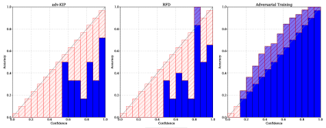
Figure 5: Relability Diagram for a Simple CNN trained on an adv-KIP dataset (left), an RFD (right), and optimized with adversarial training on CIFAR-10.

A.9 Results using modifications of adv-KIP

In this section, we present results where we modified the loss of either the inner or the outer loop of adv-KIP.

In particular, for the inner loop, we replace the cross entropy with a rescaled version of the CW loss (Carlini & Wagner, 2017), called DLR loss (Croce & Hein, 2020). Let $z$ represent the pre-softmax logits. Recall that the cross entropy loss is defined as:

$$\mathrm{CE}(x,y)=-z_{y}+\log(\sum_{i=1}^{K}e^{z_{j}})$$ (9)

Carlini & Wagner (2017) proposed to use the following (CW) loss for an attack:

$$\mathrm{CW}(x,y)=-z_{y}+\max_{i\neq y}z_{i}$$ (10)

We implement a variant of the above loss, namely the Difference of Logits Ratio (DLR) loss proposed in (Croce & Hein, 2020):

$$\mathrm{DLR}(x,y)=-\frac{z_{y}-\max_{i\neq y}z_{i}}{z_{\pi_{1}}-z_{\pi_{3}}}$$ (11)

where $\pi$ is the ordering of the components of $z$ in decreasing order (the untargeted version). This loss is invariant to scaling of the logits, and it has been used to detect cases where attacking the cross entropy loss fails due to overconfidence of the model.

For the outer loop,we incorporate the TRADES loss (Zhang et al., 2019) that aims to balance performance on clean and perturbed input points. Given a specific input $(x,y)$, TRADES optimizes over

$$\mathcal{L}(f(x;\theta),y)+\lambda\max_{x^{\prime}\in\mathcal{B}(x)}\mathcal{L}(f(x;\theta),f(x^{\prime};\theta)),$$ (12)

where $\lambda$ is a hyperparameter responsible for trading one accuracy for robustness (and vice versa). In our case, the loss reads as

$$\mathcal{L}(K_{\mathcal{X}_{T}\mathcal{X}_{S}}K_{\mathcal{X}_{S}\mathcal{X}_{S}}^{-1}\mathcal{Y}_{S},\mathcal{Y}_{T})+\lambda\max_{\mathcal{X}_{T^{\prime}}\in\mathcal{B}(\mathcal{X}_{T})}\mathcal{L}(K_{\mathcal{X}_{T}\mathcal{X}_{S}}K_{\mathcal{X}_{S}\mathcal{X}_{S}}^{-1}\mathcal{Y}_{S},K_{\mathcal{X}_{T^{\prime}}\mathcal{X}_{S}}K_{\mathcal{X}_{S}\mathcal{X}_{S}}^{-1}\mathcal{Y}_{S}).$$ (13)

Tables 11 and 12 summarize our results on neural networks trained on the modified adv-KIP datasets with $\ell_{\infty}$ attacks. We do not see any notable deviation from the results that were presented in the main text.

		Robust
Neural Net	Clean	FGSM	PGD $\ell_{\infty}$ 20	AA
Simple CNN	70.87 $\pm$ 0.44	65.06 $\pm$ 0.52	64.88 $\pm$ 0.51	0.00 $\pm$ 0.00
AlexNet	63.58 $\pm$ 5.50	47.62 $\pm$ 8.51	47.08 $\pm$ 8.65	0.11 $\pm$ 0.11
VGG11	73.72 $\pm$ 1.90	63.05 $\pm$ 4.14	62.76 $\pm$ 4.40	2.11 $\pm$ 3.28

Table 11: Test accuracies of several convolutional architectures trained on an adv-KIP CIFAR-10 DLR dataset from the FC3 kernel, with 40,000 samples. Setting: $\ell_{\infty}$, $\epsilon=8/255.$

		Robust
Neural Net	Clean	FGSM	PGD $\ell_{\infty}$ 20	AA
Simple CNN	67.39 $\pm$ 0.18	58.21 $\pm$ 0.33	58.03 $\pm$ 0.34	0.00 $\pm$ 0.00
AlexNet	59.69 $\pm$ 1.13	47.44 $\pm$ 8.00	47.08 $\pm$ 8.47	0.29 $\pm$ 0.17
VGG11	68.31 $\pm$ 1.17	60.97 $\pm$ 3.37	60.61 $\pm$ 3.46	3.58 $\pm$ 2.01

Table 12: Test accuracies of several convolutional architectures trained on an adv-KIP CIFAR-10 TRADES dataset from the FC3 kernel, with 40,000 samples. Setting: $\ell_{\infty}$, $\epsilon=8/255.$

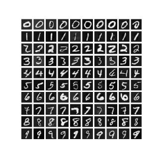
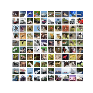
Figure 7: MNIST (left) and CIFAR-10 (right) distilled images with trained labels from an FC7 kernel.

References

- Allen-Zhu & Li (2022) Allen-Zhu, Z. and Li, Y. Feature purification: How adversarial training performs robust deep learning. In 2021 IEEE 62nd Annual Symposium on Foundations of Computer Science (FOCS), pp. 977–988. IEEE, 2022.
- Arora et al. (2019) Arora, S., Du, S. S., Hu, W., Li, Z., Salakhutdinov, R., and Wang, R. On exact computation with an infinitely wide neural net. In Wallach, H. M., Larochelle, H., Beygelzimer, A., d’Alché-Buc, F., Fox, E. B., and Garnett, R. (eds.), Advances in Neural Information Processing Systems 32: Annual Conference on Neural Information Processing Systems 2019, NeurIPS 2019, December 8-14, 2019, Vancouver, BC, Canada, pp. 8139–8148, 2019.
- Athalye et al. (2018) Athalye, A., Carlini, N., and Wagner, D. A. Obfuscated gradients give a false sense of security: Circumventing defenses to adversarial examples. In Dy, J. G. and Krause, A. (eds.), Proceedings of the 35th International Conference on Machine Learning, ICML 2018, Stockholmsmässan, Stockholm, Sweden, July 10-15, 2018, volume 80 of Proceedings of Machine Learning Research, pp. 274–283. PMLR, 2018.
- Awasthi et al. (2021) Awasthi, P., Chatziafratis, V., Chen, X., and Vijayaraghavan, A. Adversarially robust low dimensional representations. In Belkin, M. and Kpotufe, S. (eds.), Conference on Learning Theory, COLT 2021, 15-19 August 2021, Boulder, Colorado, USA, volume 134 of Proceedings of Machine Learning Research, pp. 237–325. PMLR, 2021.
- Bradbury et al. (2018) Bradbury, J., Frostig, R., Hawkins, P., Johnson, M. J., Leary, C., Maclaurin, D., Necula, G., Paszke, A., VanderPlas, J., Wanderman-Milne, S., and Zhang, Q. JAX: composable transformations of Python+NumPy programs, 2018. URL http://github.com/google/jax.
- Carlini & Wagner (2017) Carlini, N. and Wagner, D. A. Towards evaluating the robustness of neural networks. In 2017 IEEE Symposium on Security and Privacy, SP 2017, San Jose, CA, USA, May 22-26, 2017, pp. 39–57. IEEE Computer Society, 2017.
- Chen et al. (2021) Chen, W., Gong, X., and Wang, Z. Neural architecture search on imagenet in four GPU hours: A theoretically inspired perspective. In 9th International Conference on Learning Representations, ICLR 2021, Virtual Event, Austria, May 3-7, 2021. OpenReview.net, 2021.
- Croce & Hein (2020) Croce, F. and Hein, M. Reliable evaluation of adversarial robustness with an ensemble of diverse parameter-free attacks. In ICML, 2020.
- Croce & Hein (2021) Croce, F. and Hein, M. Mind the box: -apgd for sparse adversarial attacks on image classifiers. In ICML, 2021.
- Croce et al. (2020) Croce, F., Andriushchenko, M., Sehwag, V., Debenedetti, E., Flammarion, N., Chiang, M., Mittal, P., and Hein, M. Robustbench: a standardized adversarial robustness benchmark. arXiv preprint arXiv:2010.09670, 2020.
- DeGroot & Fienberg (1983) DeGroot, M. H. and Fienberg, S. E. The comparison and evaluation of forecasters. Journal of the Royal Statistical Society: Series D (The Statistician), 32(1-2):12–22, 1983.
- Deng (2012) Deng, L. The mnist database of handwritten digit images for machine learning research. IEEE Signal Processing Magazine, 29(6):141–142, 2012.
- Garg et al. (2018) Garg, S., Sharan, V., Zhang, B. H., and Valiant, G. A spectral view of adversarially robust features. In Bengio, S., Wallach, H. M., Larochelle, H., Grauman, K., Cesa-Bianchi, N., and Garnett, R. (eds.), Advances in Neural Information Processing Systems 31: Annual Conference on Neural Information Processing Systems 2018, NeurIPS 2018, December 3-8, 2018, Montréal, Canada, pp. 10159–10169, 2018.
- Goodfellow et al. (2015) Goodfellow, I. J., Shlens, J., and Szegedy, C. Explaining and harnessing adversarial examples. In Bengio, Y. and LeCun, Y. (eds.), 3rd International Conference on Learning Representations, ICLR 2015, San Diego, CA, USA, May 7-9, 2015, Conference Track Proceedings, 2015.
- Guo et al. (2017) Guo, C., Pleiss, G., Sun, Y., and Weinberger, K. Q. On calibration of modern neural networks. In International conference on machine learning, pp. 1321–1330. PMLR, 2017.
- Hashimoto et al. (2018) Hashimoto, T. B., Srivastava, M., Namkoong, H., and Liang, P. Fairness without demographics in repeated loss minimization. In Dy, J. G. and Krause, A. (eds.), Proceedings of the 35th International Conference on Machine Learning, ICML 2018, Stockholmsmässan, Stockholm, Sweden, July 10-15, 2018, Proceedings of Machine Learning Research, 2018.
- Havasi et al. (2020) Havasi, M., Jenatton, R., Fort, S., Liu, J. Z., Snoek, J., Lakshminarayanan, B., Dai, A. M., and Tran, D. Training independent subnetworks for robust prediction. arXiv preprint arXiv:2010.06610, 2020.
- He et al. (2016) He, K., Zhang, X., Ren, S., and Sun, J. Deep residual learning for image recognition. In Proceedings of the IEEE conference on computer vision and pattern recognition, pp. 770–778, 2016.
- Hendrycks & Dietterich (2019) Hendrycks, D. and Dietterich, T. G. Benchmarking neural network robustness to common corruptions and perturbations. In 7th International Conference on Learning Representations, ICLR 2019, New Orleans, LA, USA, May 6-9, 2019, 2019.
- Ilyas et al. (2019) Ilyas, A., Santurkar, S., Tsipras, D., Engstrom, L., Tran, B., and Madry, A. Adversarial examples are not bugs, they are features. In Wallach, H. M., Larochelle, H., Beygelzimer, A., d’Alché-Buc, F., Fox, E. B., and Garnett, R. (eds.), Advances in Neural Information Processing Systems 32: Annual Conference on Neural Information Processing Systems 2019, NeurIPS 2019, December 8-14, 2019, Vancouver, BC, Canada, pp. 125–136, 2019.
- Jacot et al. (2018) Jacot, A., Hongler, C., and Gabriel, F. Neural tangent kernel: Convergence and generalization in neural networks. In Bengio, S., Wallach, H. M., Larochelle, H., Grauman, K., Cesa-Bianchi, N., and Garnett, R. (eds.), Advances in Neural Information Processing Systems 31: Annual Conference on Neural Information Processing Systems 2018, NeurIPS 2018, December 3-8, 2018, Montréal, Canada, pp. 8580–8589, 2018.
- Kingma & Ba (2015) Kingma, D. P. and Ba, J. Adam: A method for stochastic optimization. In Bengio, Y. and LeCun, Y. (eds.), 3rd International Conference on Learning Representations, ICLR 2015, San Diego, CA, USA, May 7-9, 2015, Conference Track Proceedings, 2015.
- Krizhevsky (2009) Krizhevsky, A. Learning multiple layers of features from tiny images. Technical report, 2009.
- Krizhevsky et al. (2012) Krizhevsky, A., Sutskever, I., and Hinton, G. E. Imagenet classification with deep convolutional neural networks. In Pereira, F., Burges, C., Bottou, L., and Weinberger, K. (eds.), Advances in Neural Information Processing Systems, volume 25. Curran Associates, Inc., 2012.
- Kurakin et al. (2017) Kurakin, A., Goodfellow, I. J., and Bengio, S. Adversarial examples in the physical world. In 5th International Conference on Learning Representations, ICLR 2017, Toulon, France, April 24-26, 2017, Workshop Track Proceedings, 2017.
- Lakshminarayanan et al. (2017) Lakshminarayanan, B., Pritzel, A., and Blundell, C. Simple and scalable predictive uncertainty estimation using deep ensembles. Advances in neural information processing systems, 30, 2017.
- Lee et al. (2019) Lee, J., Xiao, L., Schoenholz, S., Bahri, Y., Novak, R., Sohl-Dickstein, J., and Pennington, J. Wide Neural Networks of Any Depth Evolve as Linear Models Under Gradient Descent. In Wallach, H., Larochelle, H., Beygelzimer, A., d'Alché-Buc, F., Fox, E., and Garnett, R. (eds.), Advances in Neural Information Processing Systems, volume 32. Curran Associates, Inc., 2019.
- Madry et al. (2018) Madry, A., Makelov, A., Schmidt, L., Tsipras, D., and Vladu, A. Towards Deep Learning Models Resistant to Adversarial Attacks. In International Conference on Learning Representations, 2018.
- Moosavi-Dezfooli et al. (2017) Moosavi-Dezfooli, S., Fawzi, A., Fawzi, O., and Frossard, P. Universal adversarial perturbations. In 2017 IEEE Conference on Computer Vision and Pattern Recognition, CVPR 2017, Honolulu, HI, USA, July 21-26, 2017, pp. 86–94. IEEE Computer Society, 2017.
- Naeini et al. (2015) Naeini, M. P., Cooper, G., and Hauskrecht, M. Obtaining well calibrated probabilities using bayesian binning. In Twenty-Ninth AAAI Conference on Artificial Intelligence, 2015.
- Nguyen et al. (2021a) Nguyen, T., Chen, Z., and Lee, J. Dataset meta-learning from kernel ridge-regression. In 9th International Conference on Learning Representations, ICLR 2021, Virtual Event, Austria, May 3-7, 2021. OpenReview.net, 2021a.
- Nguyen et al. (2021b) Nguyen, T., Novak, R., Xiao, L., and Lee, J. Dataset distillation with infinitely wide convolutional networks. CoRR, abs/2107.13034, 2021b.
- Niculescu-Mizil & Caruana (2005) Niculescu-Mizil, A. and Caruana, R. Predicting good probabilities with supervised learning. In Proceedings of the 22nd international conference on Machine learning, pp. 625–632, 2005.
- Novak et al. (2020) Novak, R., Xiao, L., Hron, J., Lee, J., Alemi, A. A., Sohl-Dickstein, J., and Schoenholz, S. S. Neural tangents: Fast and easy infinite neural networks in python. In 8th International Conference on Learning Representations, ICLR 2020, Addis Ababa, Ethiopia, April 26-30, 2020. OpenReview.net, 2020.
- Papernot et al. (2016) Papernot, N., McDaniel, P. D., Wu, X., Jha, S., and Swami, A. Distillation as a defense to adversarial perturbations against deep neural networks. In IEEE Symposium on Security and Privacy, SP 2016, San Jose, CA, USA, May 22-26, 2016, pp. 582–597. IEEE Computer Society, 2016. doi: 10.1109/SP.2016.41. URL https://doi.org/10.1109/SP.2016.41.
- Papernot et al. (2017) Papernot, N., McDaniel, P. D., Goodfellow, I. J., Jha, S., Celik, Z. B., and Swami, A. Practical black-box attacks against machine learning. In Karri, R., Sinanoglu, O., Sadeghi, A., and Yi, X. (eds.), Proceedings of the 2017 ACM on Asia Conference on Computer and Communications Security, AsiaCCS 2017, Abu Dhabi, United Arab Emirates, April 2-6, 2017, pp. 506–519. ACM, 2017.
- Papernot et al. (2018) Papernot, N., Faghri, F., Carlini, N., Goodfellow, I., Feinman, R., Kurakin, A., Xie, C., Sharma, Y., Brown, T., Roy, A., Matyasko, A., Behzadan, V., Hambardzumyan, K., Zhang, Z., Juang, Y.-L., Li, Z., Sheatsley, R., Garg, A., Uesato, J., Gierke, W., Dong, Y., Berthelot, D., Hendricks, P., Rauber, J., and Long, R. Technical report on the cleverhans v2.1.0 adversarial examples library. arXiv preprint arXiv:1610.00768, 2018.
- Paul et al. (2021) Paul, M., Ganguli, S., and Dziugaite, G. K. Deep learning on a data diet: Finding important examples early in training. In Ranzato, M., Beygelzimer, A., Dauphin, Y., Liang, P., and Vaughan, J. W. (eds.), Advances in Neural Information Processing Systems, volume 34, pp. 20596–20607. Curran Associates, Inc., 2021.
- Paul et al. (2022) Paul, M., Larsen, B. W., Ganguli, S., Frankle, J., and Dziugaite, G. K. Lottery tickets on a data diet: Finding initializations with sparse trainable networks. In Oh, A. H., Agarwal, A., Belgrave, D., and Cho, K. (eds.), Advances in Neural Information Processing Systems, 2022. URL https://openreview.net/forum?id=QLPzCpu756J.
- Shafahi et al. (2019) Shafahi, A., Najibi, M., Ghiasi, A., Xu, Z., Dickerson, J. P., Studer, C., Davis, L. S., Taylor, G., and Goldstein, T. Adversarial training for free! In Wallach, H. M., Larochelle, H., Beygelzimer, A., d’Alché-Buc, F., Fox, E. B., and Garnett, R. (eds.), Advances in Neural Information Processing Systems 32: Annual Conference on Neural Information Processing Systems 2019, NeurIPS 2019, December 8-14, 2019, Vancouver, BC, Canada, pp. 3353–3364, 2019.
- Simonyan & Zisserman (2015) Simonyan, K. and Zisserman, A. Very deep convolutional networks for large-scale image recognition. In International Conference on Learning Representations, 2015.
- Sinha et al. (2018) Sinha, A., Namkoong, H., and Duchi, J. C. Certifying some distributional robustness with principled adversarial training. In 6th International Conference on Learning Representations, ICLR 2018, Vancouver, BC, Canada, April 30 - May 3, 2018, Conference Track Proceedings. OpenReview.net, 2018.
- Sorscher et al. (2022) Sorscher, B., Geirhos, R., Shekhar, S., Ganguli, S., and Morcos, A. S. Beyond neural scaling laws: beating power law scaling via data pruning. In Oh, A. H., Agarwal, A., Belgrave, D., and Cho, K. (eds.), Advances in Neural Information Processing Systems, 2022. URL https://openreview.net/forum?id=UmvSlP-PyV.
- Szegedy et al. (2014) Szegedy, C., Zaremba, W., Sutskever, I., Bruna, J., Erhan, D., Goodfellow, I., and Fergus, R. Intriguing properties of neural networks, 2014.
- Tancik et al. (2020) Tancik, M., Srinivasan, P. P., Mildenhall, B., Fridovich-Keil, S., Raghavan, N., Singhal, U., Ramamoorthi, R., Barron, J. T., and Ng, R. Fourier features let networks learn high frequency functions in low dimensional domains. In Larochelle, H., Ranzato, M., Hadsell, R., Balcan, M., and Lin, H. (eds.), Advances in Neural Information Processing Systems 33: Annual Conference on Neural Information Processing Systems 2020, NeurIPS 2020, December 6-12, 2020, virtual, 2020.
- Tsilivis & Kempe (2022) Tsilivis, N. and Kempe, J. What can the neural tangent kernel tell us about adversarial robustness? In Advances in Neural Information Processing Systems. Curran Associates, Inc., 2022.
- Tsipras et al. (2019) Tsipras, D., Santurkar, S., Engstrom, L., Turner, A., and Madry, A. Robustness may be at odds with accuracy. In 7th International Conference on Learning Representations, ICLR 2019, New Orleans, LA, USA, May 6-9, 2019, 2019.
- Volpi et al. (2018) Volpi, R., Namkoong, H., Sener, O., Duchi, J. C., Murino, V., and Savarese, S. Generalizing to unseen domains via adversarial data augmentation. In Bengio, S., Wallach, H. M., Larochelle, H., Grauman, K., Cesa-Bianchi, N., and Garnett, R. (eds.), Advances in Neural Information Processing Systems 31: Annual Conference on Neural Information Processing Systems 2018, NeurIPS 2018, December 3-8, 2018, Montréal, Canada, pp. 5339–5349, 2018.
- Wang et al. (2018a) Wang, T., Zhu, J., Torralba, A., and Efros, A. A. Dataset distillation. CoRR, abs/1811.10959, 2018a.
- Wang et al. (2018b) Wang, T., Zhu, J.-Y., Torralba, A., and Efros, A. A. Dataset distillation, 2018b. URL https://arxiv.org/abs/1811.10959.
- Wenzel et al. (2020) Wenzel, F., Snoek, J., Tran, D., and Jenatton, R. Hyperparameter ensembles for robustness and uncertainty quantification. Advances in Neural Information Processing Systems, 33:6514–6527, 2020.
- Wong et al. (2020a) Wong, E., Rice, L., and Kolter, J. Z. Fast is better than free: Revisiting adversarial training. In 8th International Conference on Learning Representations, ICLR 2020, Addis Ababa, Ethiopia, April 26-30, 2020, 2020a.
- Wong et al. (2020b) Wong, E., Rice, L., and Kolter, J. Z. Fast is better than free: Revisiting adversarial training. In 8th International Conference on Learning Representations, ICLR 2020, Addis Ababa, Ethiopia, April 26-30, 2020. OpenReview.net, 2020b.
- Yuan & Wu (2021) Yuan, C.-H. and Wu, S.-H. Neural tangent generalization attacks. In Meila, M. and Zhang, T. (eds.), Proceedings of the 38th International Conference on Machine Learning, volume 139 of Proceedings of Machine Learning Research, pp. 12230–12240. PMLR, 18–24 Jul 2021.
- Zhang et al. (2019) Zhang, H., Yu, Y., Jiao, J., Xing, E. P., Ghaoui, L. E., and Jordan, M. I. Theoretically principled trade-off between robustness and accuracy. In Chaudhuri, K. and Salakhutdinov, R. (eds.), Proceedings of the 36th International Conference on Machine Learning, ICML 2019, 9-15 June 2019, Long Beach, California, USA, volume 97 of Proceedings of Machine Learning Research, pp. 7472–7482. PMLR, 2019.