AutoWeird: Weird Translational Scoring Function Identified by Random Search

Abstract

Scoring function (SF) measures the plausibility of triplets in knowledge graphs. Different scoring functions can lead to huge differences in link prediction performances on different knowledge graphs. In this report, we describe a weird scoring function found by random search on the open graph benchmark (OGB). This scoring function, called AutoWeird, only uses tail entity and relation in a triplet to compute its plausibility score. Experimental results show that AutoWeird achieves top-1 performance on ogbl-wikikg2 data set, but has much worse performance than other methods on ogbl-biokg data set. By analyzing the tail entity distribution and evaluation protocol of these two data sets, we attribute the unexpected success of AutoWeird on ogbl-wikikg2 to inappropriate evaluation and concentrated tail entity distribution. Such results may motivate further research on how to accurately evaluate the performance of different link prediction methods for knowledge graphs.

1 Introduction

Scoring function (SF), which measures the plausibility of triplets in knowledge graphs (KGs), plays an important role to learn from KGs [13, 7]. To fairly evaluate different SFs, open graph benchmark (OGB) [5] sets up leaderboards to evaluate the different models on large-scale graphs. Among the two leaderboards for link prediction task in KG, we observe that the leading models on ogbl-wikikg2 have similar forms by modeling embeddings as translations in vector spaces. To analyze the success of these SFs and try to design a better SF, we are motivated to use automated machine learning (AutoML) techniques [14, 17, 18] to search SFs in this type.

Based on the translational models [1, 12, 15, 2, 16], we first set up a search space that can cover all these translational models as special cases. Then, we conduct random search in this space to explore new designs of scoring functions. After evaluating $10$ SFs, we identified a weird SF which does not contain head entity embedding but outperforms the existing models. This is abnormal as triplets in KGs are formed by head entity, relation and tail entity. By analyzing the distribution of tail entities, we guess the success of such a weird SF may attribute to the concentrated distribution and the evaluation protocol with random negative sampling.

This tech-report is organized as follows. First, we introduce the search space, search algorithm and the training objective in Section 2. Then in Section 3, we show the the top-1 performance achieved by the weird translation-based SF on ogbl-wikikg2 and our analysis on the searched results.

2 Method

The scoring function used here is found by automated machine learning techniques (AutoML) [6, 14]. We first describe the search space where we find the scoring function (SF) in Section 2.1. And our search algorithm is introduced in Section 2.2.

2.1 Search space

Our search space is motivated by translation-based models [1, 12, 15, 2, 16] on the ogbl-wikikg2 leaderboard . Our search space is designed as follows:

• We set up the entity embeddings with two parts ${\bm{e}}_{0},{\bm{e}}_{1}$, relation embeddings with three parts ${\bm{r}}_{0},{\bm{r}}_{1},{\bm{r}}_{2}$. All these vectors have same dimension $d$, i.e. ${\bm{e}}_{0},{\bm{e}}_{1},{\bm{r}}_{0},{\bm{r}}_{1},{\bm{r}}_{2}\in\mathbb{R}^{d}$.

• The scoring function is given by combining the the different components, i.e., $s(h,r,t)=-\|f({\bm{e}}_{0}^{h},{\bm{e}}_{1}^{h},{\bm{r}}_{0},{\bm{r}}_{1},{\bm{r}}_{2},{\bm{e}}_{0}^{t},{\bm{e}}_{1}^{t})\|_{1}$, where ${\bm{e}}_{0}^{h},{\bm{e}}_{1}^{h}$ denote the embeddings for head entity $h$, ${\bm{e}}_{0}^{t},{\bm{e}}_{1}^{t}$ denote the embeddings for tail entity $t$, ${\bm{r}}_{0},{\bm{r}}_{1},{\bm{r}}_{2}$ denote the embeddings for relation $r$, and $\|\cdot\|_{1}$ is the $\ell_{1}$ norm.

• The function $f(\cdot)$ outputs a vector in $\mathbb{R}^{d}$, and is computed by adding/subtracting first-order terms (${\bm{e}}_{0}^{h},{\bm{e}}_{1}^{h},{\bm{r}}_{0},{\bm{r}}_{1},{\bm{r}}_{2},{\bm{e}}_{0}^{t},{\bm{e}}_{1}^{t}$) and/or second-order terms (element-wise product between any of these two vectors), e.g., $\bm{e}_{0}^{h}\circ\bm{e}_{1}^{t}$ and $\bm{e}_{0}^{h}\circ\bm{r}_{1}$, for entity and relation embeddings.

We can see that many translation-based SFs that are already on the OGB leaderboard [5] can all be covered in this search space. Some examples are listed in Table 1.

Table 1: Example knowledge graph embedding models that can be covered by our search space.

Model	Scoring Function
TransE [1]	$-\|{\bm{e}}_{0}^{h}-{\bm{e}}_{0}^{t}+{\bm{r}}_{0}\|$
InterHT [12]	$-\|{\bm{e}}_{0}^{h}\circ{\bm{e}}_{1}^{t}-{\bm{e}}_{1}^{h}\circ{\bm{e}}_{0}^{t}+{\bm{r}}_{0}\|$
TripleRE [15]	$-\|{\bm{e}}_{0}^{h}\circ{\bm{r}}_{1}-{\bm{e}}_{0}^{t}\circ{\bm{r}}_{2}+{\bm{r}}_{0}\|$
PairRE [2]	$-\|{\bm{e}}_{0}^{h}\circ{\bm{r}}_{1}-{\bm{e}}_{0}^{t}\circ{\bm{r}}_{2}\|$
TranS [16]	$-\|{\bm{e}}_{0}^{h}\circ{\bm{e}}_{1}^{t}-{\bm{e}}_{1}^{h}\circ{\bm{e}}_{0}^{t}+{\bm{r}}_{0}+{\bm{e}}_{0}^{h}\circ{\bm{r}}_{1}+{\bm{e}}_{0}^{t}\circ{\bm{r}}_{2}\|$
AutoWeird	$-\|-{\bm{e}}_{1}^{t}\circ{\bm{r}}_{2}+{\bm{e}}_{0}^{t}\circ{\bm{r}}_{0}+{\bm{e}}_{0}^{t}\circ{\bm{r}}_{2}-{\bm{r}}_{0}\|$

This search space covers a large number of different scoring functions. Note that with 7 different vectors ${\bm{e}}_{0}^{h},{\bm{e}}_{1}^{h},{\bm{r}}_{0},{\bm{r}}_{1},{\bm{r}}_{2},{\bm{e}}_{0}^{t},{\bm{e}}_{1}^{t}$, the total number of first-order and second-order terms is $7+7\times 7=56$. And for each of these 56 terms, we have three possible choices for its coefficient: 1, -1 and 0, where 0 coefficient means that it does not appear in $f(\cdot)$. Therefore, the total number of possible scoring functions can be as large as $3^{56}\approx 5.23\times 10^{26}$.

2.2 Search algorithm

To find new scoring functions from this search space, we consider the following bi-level optimization problem:

$$\min_{\bm{\alpha}}\mathcal{M}_{\text{val}}\left(\{{\bm{e}}(\bm{\alpha}),{\bm{r}}(\bm{\alpha})\}\right)\quad\text{s.t.}\quad\{{\bm{e}}(\bm{\alpha}),{\bm{r}}(\bm{\alpha})\}=\min_{\{{\bm{e}},{\bm{r}}\}}\mathcal{L}_{\text{tr}}(\{{\bm{e}},{\bm{r}}\};s_{\bm{\alpha}}),$$

where $\bm{\alpha}$ denotes the hyper-parameters that specify the SF $s_{\bm{\alpha}}$, $\mathcal{M}_{\text{val}}$ refers to the validation performance (e.g., MRR on the validation set), and $\mathcal{L}_{\text{tr}}$ refers to the training loss. We use the self-adversarial negative sampling loss [9], which is defined as follows:

$$\mathcal{L}(\{{\bm{e}},{\bm{r}}\};s_{\bm{\alpha}})=-\log\ \sigma(\gamma-s_{\bm{\alpha}}(h,r,t))-\sum_{i=1}^{n}\frac{1}{k}\log\ \sigma(s_{\bm{\alpha}}(h^{\prime}_{i},r,t^{\prime}_{i})-\gamma),$$ (1)

where $\gamma$ is a fixed margin, $\sigma$ is the sigmoid function, and $(h^{\prime}_{i},r,t^{\prime}_{i})$ is the $i$-th negative triplet.

For simplicity, we use random search to solve this problem. We first restrict the $f(\cdot)$ function to be computed by 5 first-order or second-order terms, and randomly choose 4 terms among all 56 terms. Then for each term, we randomly assign a coefficient 1 or -1 for it. The final function $f(\cdot)$ is computed by summing over these terms multiplied by their coefficients. We repeat the random search for 10 times. The searched SF, referred as AutoWeird, is also shown in Table 1. Different with all previous scoring functions, it only uses information from the relation ($\bm{r}_{0},\bm{r}_{2}$) and tail entity ($\bm{e}_{0}^{t}$ and $\bm{e}_{1}^{t}$) to compute the score. Intuitively, it should have bad performances as it does not consider the head entity. However, as will be demonstrated in experimental parts, it can achieve state-of-the-art performances on some KG data sets.

3 Experiments

In this section, we will first introduce the dataset. Then we will introduce implementation details, experimental results, and the post-analysis on the results.

3.1 Dataset and metric

The ogbl-wikikg2 [5] is a large KG dataset extracted from Wikidata [11]. It contains a set of triplet edges, capturing the different types of relations between entities in the world. There are $2,500,604$ entities, $535$ relation types and $17,137,181$ triplets in the whole data set.

We use original dataset splitting configuration. It splits the triplets according to time, simulating a realistic KG completion scenario that aims to fill in missing triplets that are not present at a certain timestamp. The training set contains 16,109,182 triplets, the validation set contains 429,456 triplets, and the test set contains 598,543 triplets.

Following the official guideline, we evaluate the KG embedding performance by predicting new triplet edges according to the training edges. The evaluation metric follows the standard filtered metric [1] which is widely used in KG. Specifically, each test triplet edges are corrupted by replacing its head or tail with randomly-sampled 500 negative entities, while ensuring the resulting triplets do not appear in KG. The goal is to rank the true head (or tail) entities higher than the negative entities, which is measured by Mean Reciprocal Rank (MRR).

3.2 Implementation details

In our experiments, the Adam [8] optimizer is used with a learning rate of $0.0005$. The batch size of the model is set to 512. To prevent overfitting, we use dropout technique, and set it to 0.1. The negative sampling size is set to 128. And the dimension $d$ of each embedding vector ${\bm{e}}_{0},{\bm{e}}_{1},{\bm{r}}_{0},{\bm{r}}_{1},{\bm{r}}_{2}\in\mathbb{R}^{d}$ is set to 200. The maximum number of training steps is 300,000. We validate the model every 20 thousand steps. The number of anchors for NodePiece are 20,000. And $\gamma$ in the loss function is set to 6. These hyper-parameters are selected according to the performance on the validation set.

3.3 Results

The results on ogbl-wikikg2 are shown in Table 2. By only using information from relation and tail entity, the AutoWeird model still achieves an MRR of 0.7368 on validation set and 0.7368 on test set, which outperforms all previous models on the ogbl-wikikg2 dataset. The revised version of AutoWeird model also has a performance better than all the previous methods. These counter-intuitive results demonstrate some hidden problems on the evaluation of KG embedding models. Hence, we conduct a post-analysis in the next subsection.

Table 2: Results on the ogbl-wikikg2 dataset.

Model	#Params	#Dims	Test MRR	Valid MRR
TransE [1]	1251M	500	0.4256 $\pm$ 0.0030	0.4272 $\pm$ 0.0030
RotatE [9]	1250M	250	0.4332 $\pm$ 0.0025	0.4353 $\pm$ 0.0028
PairRE [2]	500M	200	0.5208 $\pm$ 0.0027	0.5423 $\pm$ 0.0020
AutoSF [17]	500M	-	0.5458 $\pm$ 0.0052	0.5510 $\pm$ 0.0063
ComplEx [10]	1251M	250	0.5027 $\pm$ 0.0027	0.3759 $\pm$ 0.0016
TripleRE [15]	501M	200	0.5794 $\pm$ 0.0020	0.6045 $\pm$ 0.0024
ComplEx-RP [3]	250M	50	0.6392 $\pm$ 0.0045	0.6561 $\pm$ 0.0070
AutoSF + NodePiece [4]	6.9M	-	0.5703 $\pm$ 0.0035	0.5806 $\pm$ 0.0047
TripleREv2 + NodePiece [15]	7.3M	200	0.6582 $\pm$ 0.0020	0.6616 $\pm$ 0.0018
InterHT + NodePiece [12]	19.2M	200	0.6779 $\pm$ 0.0018	0.6893 $\pm$ 0.0015
TripleREv3 + NodePiece [15]	36.4M	200	0.6866 $\pm$ 0.0014	0.6955 $\pm$ 0.0008
TranS + NodePiece [16]	19.2M	200	0.6882 $\pm$ 0.0019	0.6988 $\pm$ 0.0006
AutoWeird + NodePiece	19.2M	200	0.7353 $\pm$ 0.0006	0.7362 $\pm$ 0.0006
EntOccur	-	-	0.4419	0.4467

Table 3: Results on the ogbl-biokg dataset.

Model	#Params	#Dims	Test MRR	Valid MRR
TransE [1]	188M	500	0.7452 $\pm$ 0.0004	0.7456 $\pm$ 0.0003
RotatE [9]	188M	250	0.7989 $\pm$ 0.0004	0.7997 $\pm$ 0.0002
ComplEx [10]	188M	250	0.8095 $\pm$ 0.0007	0.8105 $\pm$ 0.0001
PairRE [2]	188M	200	0.8164 $\pm$ 0.0005	0.8172 $\pm$ 0.0005
AutoSF [17]	93.8M	-	0.8309 $\pm$ 0.0008	0.8317 $\pm$ 0.0007
TripleRE [15]	470M	200	0.8348 $\pm$ 0.0007	0.8360 $\pm$ 0.0006
ComplEx-RP [3]	188M	1000	0.8492 $\pm$ 0.0002	0.8497 $\pm$ 0.0002
AutoBLM+KGBench [18]	192M	-	0.8536 $\pm$ 0.0003	0.8548 $\pm$ 0.0002
AutoWeird	376M	500	0.6755 $\pm$ 0.0004	0.6752 $\pm$ 0.0003
EntOccur	-	-	0.3387	0.3387

3.4 Post-analysis: why AutoWeird is effective?

To analyze why AutoWeird is effective, we first count the occurrence of tail entities after adding inverse relations to the data set. Specifically, for each entity, we count how many times it appears as the tail entity in the training set. As is shown in Figure 1(a), a few number of entities has more than one million occurrences in the training set. Such a concentrated distribution also exists in the test triplets (Figure 1(b)), leading to a strong bias to the high occurrence entities.

Note that the evaluation protocol in ogbl-wikikg2 is to rank the positive tail entities over a set of 500 randomly sampled negative entities. Hence, the bias will become more severe during evaluation. As in Figure 1(a) and 1(b), if we only randomly sample $500$ entities from $10^{6}$ entities, the majority of them will has low occurrence.

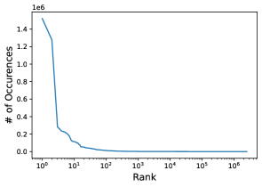
(a) Training set of ogbl-wikikg2.

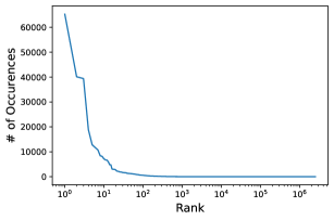
(b) Testing set of ogbl-wikikg2.

(c) Training set of ogbl-biokg.

(d) Testing set of ogbl-biokg.

Figure 1: Tail entity occurrence distribution for different KG data sets.

Based on these observations, we design a simple method, named as EntOccur, by using the occurrence as scores. For each triplet $(h,r,t)$ in the training set, we count the occurrence of entities $t$ for each relation $r$. Then the score of $(h,r,t)$ in inference is directly set as the occurrence of $t$ with respect to the specific relation $r$. As in Table 2, such a simple model EntOccur outperforms some embedding models like TransE and RotatE.

We further evaluate the searched SF AutoWeird and the simple solution EntOccur on the other KG link prediction dataset ogbl-biokg [5]. By comparing the performance of AutoWeird and EntOccur with the results on the leaderboard in Table 3, AutoWeird and EntOccur are much worse. By comparaing ogbl-biokg with ogbl-wikikg2, we find that

• the distributions of tail entity occurrence in ogbl-biokg in Figure 1(c) and 1(d) are not as concentrated as those of ogbl-wikikg2 in Figure 1(a) and 1(b);

• the number of entities in ogbl-biokg is $93,773$, much smaller than ogbl-wikikg2 with $2,500,604$;

• the negative samples for evaluation in ogbl-biokg have the same type with the positive tail entity.

Hence, the negative entities in ogbl-biokg have higher correlation with the positive tail entity than ogbl-wikikg2, alleviating the bias towards entities with high occurrence. As such, we attribute the success of AutoWeird in ogbl-wikikg2 to the inappropriate evaluation protocol.

In conclusion, these results show that there is a relatively strong correlation between relations and a few high occurrence entities in ogbl-wikikg2. And the correlation may lead to the weird scoring function, AutoWeird in Table 1. A better way to compare the different models may be (1) using the full set of negative entities, or (2) using some highly correlated negative entities, or (3) using the larger number of negative entities rather than $500$ randomly sampled ones. However, due to the time complexity in evaluating millions of negative entities for each triplet in ogbl-wikikg2, we leave it as a future work.

4 Conclusion

In this paper, we propose a novel search space for the scoring function in knowledge graph embedding model. We find a novel scoring function from this search space by random search, which only depends on tail entity and relation. Empirical results on the ogbl-wikikg2 dataset demonstrate that the searched scoring function is able to achieve state-of-the-art results among all previous models. These strange results should motivate us to consider potential problems on the evaluation of KG embedding models.

References

- [1] A. Bordes, N. Usunier, A. Garcia-Duran, J. Weston, and O. Yakhnenko. Translating embeddings for modeling multi-relational data. Advances in neural information processing systems, 26, 2013.
- [2] L. Chao, J. He, T. Wang, and W. Chu. Pairre: Knowledge graph embeddings via paired relation vectors. arXiv preprint arXiv:2011.03798, 2020.
- [3] Y. Chen, P. Minervini, S. Riedel, and P. Stenetorp. Relation prediction as an auxiliary training objective for improving multi-relational graph representations. arXiv preprint arXiv:2110.02834, 2021.
- [4] M. Galkin, J. Wu, E. Denis, and W. L. Hamilton. Nodepiece: Compositional and parameter-efficient representations of large knowledge graphs. arXiv preprint arXiv:2106.12144, 2021.
- [5] W. Hu, M. Fey, M. Zitnik, Y. Dong, H. Ren, B. Liu, M. Catasta, and J. Leskovec. Open graph benchmark: Datasets for machine learning on graphs. arXiv preprint arXiv:2005.00687, 2020.
- [6] F. Hutter, L. Kotthoff, and J. Vanschoren. Automated machine learning: methods, systems, challenges. Springer Nature, 2019.
- [7] S. Ji, S. Pan, E. Cambria, P. Marttinen, and S. Y. Philip. A survey on knowledge graphs: Representation, acquisition, and applications. IEEE Transactions on Neural Networks and Learning Systems, 2021.
- [8] D. P. Kingma and J. Ba. Adam: A method for stochastic optimization. arXiv preprint arXiv:1412.6980, 2014.
- [9] Z. Sun, Z.-H. Deng, J.-Y. Nie, and J. Tang. Rotate: Knowledge graph embedding by relational rotation in complex space. arXiv preprint arXiv:1902.10197, 2019.
- [10] T. Trouillon, C. R. Dance, Éric Gaussier, J. Welbl, S. Riedel, and G. Bouchard. Knowledge graph completion via complex tensor factorization. Journal of Machine Learning Research, 18(130):1–38, 2017.
- [11] D. Vrandečić and M. Krötzsch. Wikidata: a free collaborative knowledgebase. Communications of the ACM, 57(10):78–85, 2014.
- [12] B. Wang, Q. Meng, Z. Wang, D. Wu, W. Che, S. Wang, Z. Chen, and C. Liu. Interht: Knowledge graph embeddings by interaction between head and tail entities. arXiv preprint arXiv:2202.04897, 2022.
- [13] Q. Wang, Z. Mao, B. Wang, and L. Guo. Knowledge graph embedding: A survey of approaches and applications. TKDE, 29(12):2724–2743, 2017.
- [14] Q. Yao and M. Wang. Taking human out of learning applications: A survey on automated machine learning. arXiv preprint arXiv:1810.13306, 2018.
- [15] L. Yu, Z. Luo, D. Lin, H. Liu, and Y. Deng. Triplere: Knowledge graph embeddings via triple relation vectors. arXiv preprint arXiv:2112.0095, 2021.
- [16] X. Zhang, Q. Yang, and D. Xu. Trans: Transition-based knowledge graph embedding with synthetic relation representation. arXiv preprint arXiv:2204.08401, 2022.
- [17] Y. Zhang, Q. Yao, W. Dai, and L. Chen. Autosf: Searching scoring functions for knowledge graph embedding. In 2020 IEEE 36th International Conference on Data Engineering (ICDE), pages 433–444. IEEE, 2020.
- [18] Y. Zhang, Q. Yao, and J. T. Kwok. Bilinear scoring function search for knowledge graph learning. IEEE Transactions on Pattern Analysis and Machine Intelligence, 2022.