Degree Centrality Algorithms For Homogeneous Multilayer Networks

Abstract

Centrality measures for simple graphs/networks are well-defined and each has numerous main-memory algorithms. However, for modeling complex data sets with multiple types of entities and relationships, simple graphs are not ideal. Multilayer networks (or MLNs) have been proposed for modeling them and have been shown to be better suited in many ways. Since there are no algorithms for computing centrality measures directly on MLNs, existing strategies reduce (aggregate or collapse) the MLN layers to simple networks using Boolean AND or OR operators. This approach negates the benefits of MLN modeling as these computations tend to be expensive and furthermore results in loss of structure and semantics.
      In this paper, we propose heuristic-based algorithms for computing centrality measures (specifically, degree centrality) on MLNs directly (i.e., without reducing them to simple graphs) using a newly-proposed decoupling-based approach which is efficient as well as structure and semantics preserving. We propose multiple heuristics to calculate the degree centrality using the network decoupling-based approach and compare accuracy and precision with Boolean OR aggregated Homogeneous MLNs (HoMLN) for ground truth. The network decoupling approach can take advantage of parallelism and is more efficient compared to aggregation-based approaches. Extensive experimental analysis is performed on large synthetic and real-world data sets of varying characteristics to validate the accuracy and efficiency of our proposed algorithms.

1 Introduction

In graph-based applications, an important requirement is to measure the importance of a node/vertex, which can translate to meaningful real-world inferences on the data set. For example, cities that act as airline hubs, people on social networks who can maximize the reach of an advertisement/tweet/post, identification of mobile towers whose malfunctioning can lead to the maximum disruption, and so on. Centrality measures include degree centrality [Bródka et al., 2011], closeness centrality [Cohen et al., 2014], eigenvector centrality [Solá et al., 2013], stress centrality [Shi and Zhang, 2011], betweenness centrality [Brandes, 2001], harmonic centrality[Boldi and Vigna, 2014], and PageRank centrality [Pedroche et al., 2016], are some of the well-defined and widely-used local and global centrality measures.

These centrality measurements use a set of criteria to determine the importance of a node or edge in a graph. Degree centrality metric measures the importance of a node in a graph in terms of its degree, which is the number of 1-hop neighbors a node has in the graph. Most centrality metrics are clearly defined for simple graphs or monographs, and there are numerous techniques for calculating them on simple graphs. However, for modeling complex data sets with multiple types of entities and relationships, multilayer networks have been shown to be a better alternative due to the clarity of representation, ability to preserve the structure and semantics of different types of information for the same set of nodes, and support for parallelism [Kivelä et al., 2014, Santra et al., 2017b, Fortunato and Castellano, 2009].

A multilayer network [De Domenico et al., 2013] is made up of layers, each of which is a simple graph with nodes (that correspond to entities) and edges (that correspond to relationships). Nodes within a layer are connected (intra-layer edges) based on a relationship between nodes. Nodes in a layer may also be optionally connected to nodes in other layers through inter-layer edges. As an example, the diverse interactions among the same set of people across different social media (such as Facebook, LinkedIn, and Twitter) can be modeled using a multilayer network (see Figure 1.) Because the entities in each layer are the same, but the relationships in each layer are different (Facebook-friends, Twitter-relationships, LinkedIn-connections), this sort of MLN is referred to as homogeneous MLNs (or HoMLNs). As the edges between layers are implicit, they are not shown. It is also feasible to build MLNs with different types of entities and relationships within and between layers. This form of heterogeneous MLNs (or HeMLNs) is required for modeling, for example, the DBLP data set [dbl,] with authors, articles, and conferences [Kivelä et al., 2014]. Hybrid Multilayer networks (HyMLNs) include both types of layers.

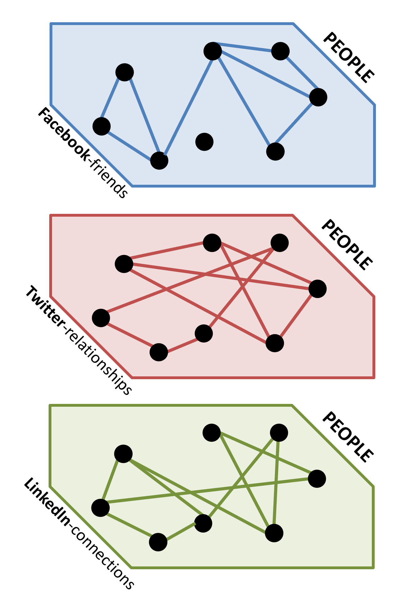
Figure 1: Social Media HoMLN Example

For a social-network HoMLN such as the one shown in Figure 1, it will be interesting to find out the set of people who are the most influential in a single network or across multiple (or a subset of) social networks. This corresponds to finding out the centrality nodes of an MLN using corresponding one or more layers. Extant algorithms that calculate centrality measures on multilayer networks are limited to simple graphs/networks and lead to the loss of structure and semantics when reduction is used. This paper presents heuristic-based algorithms for computing degree centrality nodes (or DC nodes) on HoMLNs directly with high accuracy/precision and efficiency. Boolean OR composition of layers is used for ground truth in this paper.

For comparing the accuracy of the decoupling-based algorithm, we use Boolean operators for aggregation of layers and use simple graph algorithms on them for ground truth. Other types of aggregations are also possible. The aggregation of layers using AND and OR Boolean operators for homogeneous MLNs are straightforward as the nodes are the same in each layer and the operator semantics are applied to the edges. Both AND and OR operators are commutative and distributive. OR aggregation is likely to increase the size of the graph (number of edges) used for ground truth. Accuracy is computed by comparing the ground truth results for the graph with the results obtained by the decoupling-based algorithm for the layers of the same graph. The naive algorithm uses only the results of each layer and applies the operators to the results. Typically, the naive approach does not yield good accuracy requiring additional information from each layer to be retained and used for the composition algorithm using heuristics. As layers are processed independently (may be in parallel), no information about the other layer is assumed while processing a layer.

We adapt the decoupling-based approach proposed in  [Santra et al., 2017a, Santra et al., 2017b] for our algorithms. Based on this approach, we compute centrality on each layer independently once and keep minimal additional information from each layer for composing. With this, we can efficiently estimate the degree centrality (DC) nodes of the HoMLN. This approach has been shown to be application independent, efficient, lends itself to parallel processing (of each layer), and is flexible for computing centrality measures on any subset of layers. The naive approach to which we compare our proposed heuristic-based accuracy retains no additional information from the layers apart from the degree centrality nodes and their values. Contributions of this paper are:

• Algorithms for directly computing degree centrality nodes of Homogeneous MLNs (HoMLNs.)

• Several heuristics to improve accuracy, precision, and efficiency of computed results.

• Decoupling-based approach to preserve structure and semantics of MLNs.

• Experimental analysis on large number of synthetic and real-world graphs with diverse characteristics.

• Accuracy, Precision, and Efficiency comparisons with ground truth and naive approach.

The rest of the paper is organized as follows: Section 2 discusses related work. Section 3 introduces the decoupling approach for MLN analysis and discusses its advantages and challenges. Section 4 discusses ground truth and naive approach to degree centrality. Sections 5, and 6 describe composition-based degree centrality computation for HoMLNs using heuristics for accuracy and precision, respectively. Section 7.1 describes the experimental setup and the data sets. Section 7.2 discusses result analysis followed by conclusions in Section 8.

2 Related Work

Because complex and massive real-world data sets are becoming more popular and accessible, there is a pressing need to describe them as graphs and analyze them in various ways. However, the use of MLN for modeling poses additional challenges in terms of computing centrality measures on MLNs instead of simple graphs. Centrality measures including MLN centrality shed light on various properties of the network. Although there have been numerous studies on recognizing central entities in simple graphs, there have been few studies on detecting central entities in multilayer networks. Existing research for finding central entities in multilayer networks is use-case specific, and there is no standard paradigm for addressing the problem of detecting central entities in a multilayer network.

Degree centrality is the most common and widely-used centrality measure. Degree centrality is used to identify essential proteins [Tang et al., 2013]. It is also used in identifying epidemics in animals [Candeloro et al., 2016] and the response of medication in children with epilepsy [Wang et al., 2021]. The most common and prominent use of degree centrality is in the domain of social network analysis. Some of the common use of degree centrality in social network analysis is identifying the most influential node [Srinivas and Velusamy, 2015], influential spreaders of information [Liu et al., 2016], finding opinion leaders in a social network [Risselada et al., 2016], etc.

Despite being one of the most common and widely used centrality measures, very few algorithms or solutions exist to directly calculate the degree centrality of an MLN. In this study [Bródka et al., 2011], the author proposes a solution to find degree centrality in a 10-layer MLN consisting of the Web 2.0 social network dataset. Similar to the previous work, in [Rachman et al., 2013], authors identify the degree centrality of nodes using the Kretschmer method. The authors in this study [Yang et al., 2014] proposed a node prominence profile-based method to effectively predict the degree centrality in a network. In another study [Gaye et al., 2016], authors propose a solution to find the top-K influential person in an MLN social network using diffusion probability. More recently there has been some work in developing algorithms for MLNs using the decoupling-based approach [Santra et al., 2017b].

The majority of degree centrality computation algorithms are main memory based and are not suitable for large graphs. They are also use-case specific. The authors adapt a decoupling-based technique proposed in [Santra et al., 2017b] for MLNs, where each layer can be analyzed individually and in parallel, and graph characteristics for a HoMLN can be calculated utilizing the information gathered for each layer. Our algorithms follow the network decoupling methodology, which has been demonstrated to be efficient, flexible, and scalable. Achieving desired accuracy/precision/recall, however, is the challenge. Our approach is not strictly main-memory based as each layer outputs results into a file which are used for the decomposition algorithm. Also, as each layer is likely to be smaller than the OR aggregation of layers, larger size MLNs can be accommodated in our approach.

3 Network Decoupling Approach

Existing multilayer network analysis approaches convert or transform an MLN into a simple graph . Aggregating or projecting the network layers into a simple graph accomplishes this. Edge aggregation is used to bring homogeneous MLNs together into a simple graph. Although aggregating an MLN into a simple network enables the use of currently available techniques for centrality and community discovery (of which there are many), the MLN’s structure and semantics are not retained, causing information loss.

We use the network decoupling strategy for MLN analysis to overcome the aforementioned difficulties. Figure 2 shows the proposed network decoupling strategy. It entails determining two functions: one for analysis ($\Psi$) and the other for composition ($\Theta$). Each layer is analyzed independently using the analysis function (and in parallel). The partial results (as defined by the MLN) from each of the two layers are then combined using a composition function/algorithm to obtain the HoMLN results for the two layers. MLNs with more than two layers can use this binary composition repeatedly. Independent analysis permits the use of existing techniques for each layer. Decoupling, on the other hand, increases efficiency, flexibility, and scalability along with extending the existing graph analysis algorithms to compute directly on MLNs.

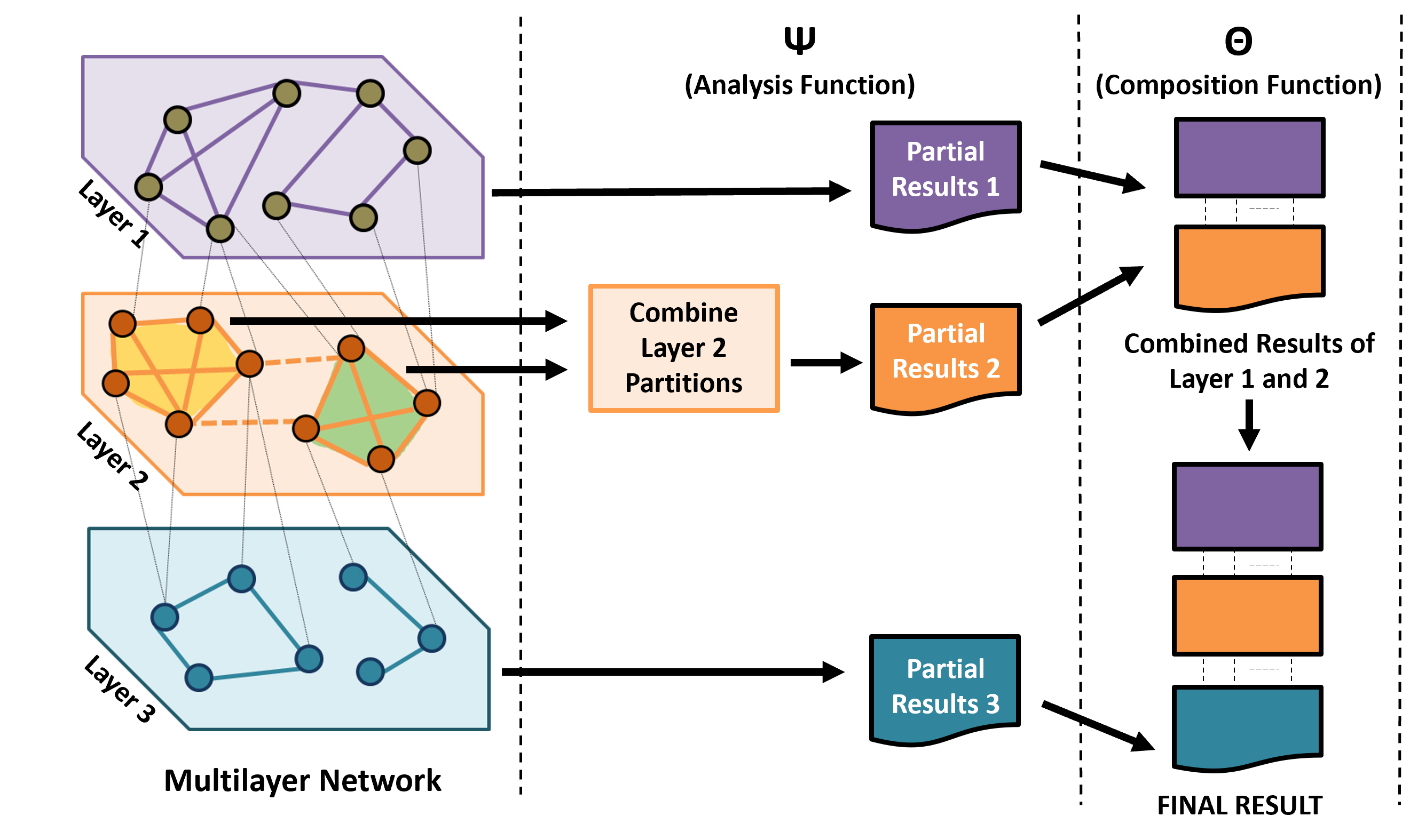
Figure 2: Overview of the network decoupling approach.

As the network decoupling method preserves the structure and semantics of the data, drill-down and visualization of final results are easy to support. Each layer (or graph) is likely to be smaller, consume less memory than the whole MLN, and composition is done separately. The analysis function results are preserved and used in the composition. The requirement to recompute is reduced because the result of a single analysis function can be used by several composition functions, increasing the efficiency of the decoupling-based approach. Individual layers can be analyzed using any of the available simple graph centrality algorithms. This method is also application-independent. As a result, the decoupling-based approach can be used to extend existing centrality algorithms to MLNs. To compose the outputs of analysis functions (partial results) into the final results, we only need to define the composition function.

One of the major challenges with the decoupling approach is to determine the minimum additional information to retain as part of the layer analysis step to be used during composition to improve the overall accuracy with respect to the ground truth. For many composition algorithms we have looked into, there is a trade-off between using more information from each layer and improving accuracy. This trade-off is demonstrated in this paper for one of the heuristics.

The decoupling approach’s layer-wise analysis has a number of advantages. First, only a smaller layer of the network needs to be loaded into memory, rather than the whole network. Second, the analysis of individual layers can be parallelized, reducing the algorithm’s overall execution time. Finally, the composition function ($\Theta$) relies on intuition, which is built into the heuristic and takes substantially less calculation than $\Psi$.

The accuracy of an MLN analysis algorithm is determined by the information we keep (in addition to the output) during individual layer analysis. The basic minimum information we may maintain from each layer in terms of centrality measurements is the high centrality nodes of that layer, as well as their centrality values. The accuracy should potentially improve as we retain more relevant data for composition. However, determining what is relevant and should be retained to improve accuracy is the main challenge of this approach. The key hurdles are identifying the most beneficial minimal information and the intuition for their effectiveness.

4 Degree Centrality for MLNs

The degree of a node in a graph is the total number of edges that are incident on it. Degree hubs are nodes in a network that have a degree larger than or equal to the network’s average degree. Degree hubs are specified for simple graphs. In [abhishek_hubify], the authors have proposed three algorithms to estimate degree hubs in AND composed multilayer networks. However, there are no algorithms for calculating degree hubs for OR composed HoMLNs. If the HoMLN layers are composed of a Boolean operation such as OR, we can expand the notion of a hub from a simple graph to HoMLNs. In this paper, we suggest various composition functions to maximize accuracy, precision, and efficiency while estimating degree hubs in OR composed multilayer networks.

The ground truth is used to evaluate the performance and accuracy of our suggested heuristics for detecting the degree hubs of a multilayer network.

The degree centrality of a vertex $u$ in a network is defined as $C_{D}(u)=\textit{Number of adjacent neighbors}$. This value is divided by the maximum number of edges a vertex can have to normalize it. The equation for normalized degree centrality is:

$$C_{D}(v)=\frac{degree(v)}{n-1}$$ (1)

High centrality hubs or degree hubs are the vertices with normalized degree centrality values higher than the other vertices.

Even though there are different variations of degree centrality such as the group degree centrality [Everett and Borgatti, 1999], time scale degree centrality [Uddin and Hossain, 2011], and complex degree centrality [Kretschmer and Kretschmer, 2007], in this paper, we only address the normalized degree centrality for Boolean OR composed undirected homogeneous multilayer networks. We propose several algorithms to identify high centrality degree hubs in Boolean OR composed MLNs. We test the accuracy and efficiency of our algorithm against the ground truth. With extensive experiments on data sets of varying characteristics, we show that our approaches perform better than the naive approach and are efficient compared to the ground truth.

For degree centrality, the ground truth is calculated as follows:

• First, all the layers of the network are aggregated into a single layer using the Boolean OR composition function.

• Degree centrality of the aggregated graphs is calculated and the hubs are identified.

We compare the hubs computed by our algorithms against ground truth for accuracy and/or precision. We use Jaccard’s coefficient as the measure to compare the accuracy of our solutions with the ground truth.

Our aim is to design heuristics based on intuition and algorithms using the network decouple approach so that our accuracy for degree centrality is much better than the naive approach and closer to the ground truth. Efficiency is expected be better than that of the ground truth. For the naive composition approach, we estimate the degree hubs in OR composed layers as the union of the degree hubs of the individual layers (for OR aggregation). Even though our solution works for any arbitrary number of layers, we have focused on two layers due to its cascading effect for higher number of layers.

5 Degree Centrality Heuristics for Accuracy

We measure accuracy with respect to ground truth using the Jaccard coefficient. An accuracy of 1 indicates an exact match with the ground truth without any false positives or false negatives. The goal is to get accuracy as close to 1 as possible using the decoupling approach. For most applications, high accuracy is desired. In this section, we present two heuristic-based composition algorithms with better overall accuracy as compared to the naive approach.

5.1 Degree Centrality Heuristic Accuracy 1 (DC-A1)

Intuitively, with the information from each layer, we are trying to estimate the degree of a node when the layers are aggregated. If we can do it effectively, we can use the approximated average degree of the OR aggregation to determine whether a node is a hub when layers are combined. Based on the OR operator semantics, the estimated degree $estDeg_{xORy}(u)$ of a node $u$ in the OR composed layer can be $max(deg_{x}(u),deg_{y}(u))$. This happens when the one-hop neighbor of the node $u$ in layer $x$ is a subset of the one-hope neighbor of the same node in layer $y$ or vice-versa. We can use this estimated degree value of the nodes to directly calculate the degree hubs of the HoMLN in the OR composed layer. The algorithm 1 describes the steps of the composition or $\Theta$ step using this heuristic.

Algorithm 1 Procedure for Heuristic DC-A1

Require: $deg_{x}$, $deg_{y}$, $DHxORy\leftarrow\emptyset$

1:for $u\in x$ do

2:     $estDeg_{xORy}(u)\leftarrow max(deg_{x}(u),deg_{y}(u))$

3:end for

4:Calculate $DH{{}^{\prime}}_{xORy}$ using $estDeg_{xORy}(u)$

As can be seen from Table 1 and Figure 3, this heuristic improves accuracy for data sets where the edge distribution is equal and further accuracy improves as the data set size increases. This is as expected as equal distribution of edges provides a better estimated degree for the combined layers. And for data sets with a larger number of edges, even with non-equal distribution, the average degree of the combined layers is smoother than for small data sets. This observation holds for the other synthetic data sets as well. For real-world data sets, both DC-A1 and DC-A2 are uniformly significantly better than the naive and do not deviate much from synthetic data sets with wider coverage of edge distributions and degree distributions.

5.2 Degree Centrality Heuristic Accuracy 2 (DC-A2)

In the DC-A1 heuristic, we assumed that the one-hop neighbors of a node $u$ in layer $x$ are going to be a subset of one-hop neighbors of the same node in layer $y$ or vice-versa. When we are estimating the degree of a node $u$ in the OR composed layer, there is a minimum value and maximum value for the estimated degree value of that node. The minimum of the estimated degree value is $max(deg_{x}(u),deg_{y}(u))$. Similarly, the maximum value of the estimated degree could be $min(((deg_{x}(u)+deg_{y}(u)),(n-1))$ when there is no common one-hop neighbour among layer $x$ and $y$ for node $u$. Here $n$ is the number of nodes in each layer of the HoMLN. Based on observations of various datasets, the estimated degree of a node $u$ in the OR composed layers is neither the possible minimum nor possible maximum value, rather somewhere close to the average of these values. Thus, we estimate the estimated degree of node $u$ in the OR composed layer, $estDeg_{xORy}(u)$, as the average of $max(deg_{x}(u),deg_{y}(u))$ and $min(((deg_{x}(u)+deg_{y}(u)),(n-1))$. We then use the $estDeg_{xORy}(u)$ of the nodes to calculate the degree hubs of the OR composed layer.

Note that in this heuristic, we are not using any additional information than heuristic DC-A1, but changing our estimation to a more meaningful, realistic value than taking an extreme. With this simple change in the heuristic, again from Table 1 and Figure 3, one can see a significant improvement in accuracy over DC-A1. In fact, some of the accuracies reach as high as 0.98 which is as good as 1. One can also see that the edge distribution and data set size differences no longer have the kind of impact seen in DC-A1. also, real-world data sets match the synthetic ones to some extent.

6 Degree Centrality Heuristics for Precision

As mentioned in the previous section, we use the Jaccard coefficient as a measure of accuracy to compare the performance of our heuristics. Based on use cases, the Jaccard coefficient might not be the only measure for many real-world applications. For example, An airline is trying to expand its operation to a new city based on the air route and operation of other competitors. This problem can be modeled as a problem to find the degree hubs of a HoMLN where each node of the HoMLN is a city and each layer represent the route of the competitors among these cities. In this scenario, a high precision algorithm is preferred as a false positive in identifying a hub might lead the airline to expand to a city without much traffic and incur loss due to the expansion. Advertising on multiple social networks also has a similar need to avoid false positives. Hence, in general, it is meaningful to identify heuristics that do not produce any false positives or any false negatives depending upon the application’s need. In this section, we provide two heuristic-based composition algorithms to find the degree hubs of a HoMLN with high precision.

6.1 Degree Centrality Heuristic Precision 1 (DC-P1)

For the Boolean OR operator composed ground-truths, if a node is a degree hub (DH) in layer $x$ or layer $y$, then it is likely that the node is going to be a degree hub in the OR composed ground truth. We use this intuition as the basis for heuristic DC-P1 which is used to develop the first composition algorithm for the $\Theta$ function to compute high precision degree hubs.

As we previously mentioned, in the analysis function $(\Psi)$ of the decoupling approach we analyze the layers of the HoMLN and use the partial results and additional information to obtain the final results for the MLN. In DC-P1, after the analysis $(\Psi)$ phase of each layer (say layer $x$), we keep the set of degree hubs $DH_{x}$, the average degree $avgDeg_{x}$, and the set of one-hop neighbors of each degree hub (say, $u$) $NBD_{x}(u)$.

Table 1: Summary of Synthetic Data Set-1

Base Graph	GID	Edge Dist. %	#Edges
#Nodes, #Edges		in Layers	L1	L2	L1 OR L2
100KV, 500KE	1	70,30	350000	150000	499587
	2	60,40	200000	300000	499505
	3	50,50	250000	250000	499505
100KV, 1ME	4	70,30	700000	300000	998303
	5	60,40	600000	400000	998176
	6	50,50	500000	500000	997998
100KV, 2ME	7	70,30	600000	1400000	1993608
	8	60,40	1200000	800000	1992855
	9	50,50	1000000	1000000	1992207
300KV, 1.5ME	10	70,30	1050000	450000	1499463
	11	60,40	900000	600000	1499425
	12	50,50	750000	750000	1499347
300KV, 3ME	13	70,30	2100000	900000	2997825
	14	60,40	1800000	1200000	2997627
	15	50,50	1500000	1500000	2997538
300KV, 6ME	16	70,30	4200000	1800000	5991761
	17	60,40	3600000	2400000	5990599
	18	50,50	3000000	3000000	5990044
500KV, 2.5ME	19	70,30	1750000	750000	2499344
	20	60,40	1500000	1000000	2499238
	21	50,50	1250000	1250000	2499166
500KV, 5ME	22	70,30	3500000	1500000	4997388
	23	60,40	3000000	2000000	4996910
	24	50,50	2500000	2500000	4997209
500KV, 10ME	25	70,30	7000000	3000000	9989402
	26	60,40	6000000	4000000	9989190
	27	50,50	5000000	5000000	9987447

During the $\Theta$ step, we use the stored partial results and additional information to estimate the hubs for two layers (say layer $x$ and layer $y$). As for the OR composed ground-truth graph, the number of edges for a node is likely to increase. We can estimate the average degree of the OR composed layer, $avgEstDeg_{xORy}$, to be the maximum between $avgDeg_{x}$ and $avgDeg_{y}$. For each node present in either $DH_{x}$ or $DH_{y}$, if the union of their one-hop neighbors set is more than $avgEstDeg_{xORy}$, we consider that node a degree hub in the OR composed layer of $x$ and $y$. Algorithm 2 shows the detailed steps of the composition algorithm ($\Theta$.)

Algorithm 2 Procedure for $\Theta$ using Heuristic DC-P1

Require: $DH_{x}$, $avgDeg_{x}$, $DH_{y}$, $avgDeg_{y}$, $NBD_{x}$, $NBD_{y}$, $DH_{xORy}\leftarrow\emptyset$

1:$avgEstDeg_{xORy}\leftarrow max(avgDeg_{x},avgDeg_{y})$

2:for $u\in DH_{x}\cup DH_{y}$ do

3:     if $|NBD_{x}(u)\cup NBD_{y}(u)|>=avgEstDeg_{xORy}$ then

4:         $DH{{}^{\prime}}_{xORy}\leftarrow DH{{}^{\prime}}_{xORy}\cup u$

5:     end if

6:end for

Degree hubs and their values for each layer allow us to compute the higher bound of the average for the aggregated graph. One-hop neighbor information is used to reduce or eliminate false positives. However, as these are retained only for hubs, information is still not complete. Even with this limited additional information, as we will see in the experimental section (Section 7.2), there is a significant improvement in precision over the naive for all data sets. For the synthetic data sets, we get a precision of 100% and for the real-world data sets we get a mean precision of 96% (Refer to Section 7.2).

6.2 Degree Centrality Heuristic Precision 2 (DC-P2)

Based on how the edges are distributed in the layers of an MLN, the actual average degree of the OR composed ground truth, $avgDeg_{xORy}$, of layers $x$ and $y$ might differ from the estimated $avgEstDeg_{xORy}$ in DC-P1. If the $avgEstDeg_{xORy}$ is substantially greater than $avgEstDeg_{xORy}$, then a lot of nodes will not be included as a hub in the OR composed layer despite having enough common neighbors across both layers $x$ and $y$. Similarly, if $avgEstDeg_{xORy}$ is smaller than $avgEstDeg_{xORy}$, a lot of false positives will be generated as hubs in the OR composed layer.

To better estimate the $avgEstDeg_{xORy}$, we keep the degree of each node from each layer as additional information during the $\Psi$ step. This allows us to estimate the individual degree of a node $u$ in the OR composed layer from its degree information in layer $x$ and layer $y$. If the degree of a node $u$ in layer $x$ is $deg_{x}(u)$ and degree of the same node in layer $y$ is $deg_{y}(u)$, then estimated degree of node $u$ in the OR composed layer, $estDeg_{xORy}(u)$, is going to be $max(deg_{x}(u),deg_{y}(u))$. Using the estimated degree $estDeg_{xORy}(u)$ of each node $u$, we calculate the $avgEstDeg_{xORy}$. The rest of the steps of the algorithm are same as 2.

7 Experimental Analysis

7.1 Data Sets and Environment

Table 2: Summary of Real World Data Set

Base Graph	GID	Edge Dist. %	#Edges
#Nodes, #Edges		in Layers	L1	L2	L1 OR L2
735KV, 2.6ME	amazon-2008_1	50,50	1306357	1304863	1958865
	amazon-2008_2	70,30	1828100	784552	2063141
	amazon-2008_3	90,10	2349969	261133	2376256
325KV, 1.7ME	cnr-2000_1	50,50	876444	876383	1314919
	cnr-2000_2	70,30	1226781	525244	1384962
	cnr-2000_3	90,10	1577646	175236	1595367
100KV, 1.5ME	uk-2007-05_1	50,50	759899	761252	1141215
	uk-2007-05_2	70,30	1065435	455957	1202326
	uk-2007-05_3	90,10	1369767	152167	1385013

The NetworkX [Hagberg et al., 2008] package is used in our Python implementation. The experiments were carried out on a single node SDSC Expanse [Towns et al., 2014]. Each node in the cluster runs the CentOS Linux operating system using an AMD EPYC 7742 CPU with 128 cores and 256GB of RAM hardware. Both synthetic and real-world data sets were used to evaluate the proposed methodologies. PaRMAT [Khorasani et al., 2015], a parallel version of the popular graph generator RMAT [Chakrabarti et al., 2004], which uses the Recursive-Matrix-based graph generation technique, was used to create the synthetic data sets.

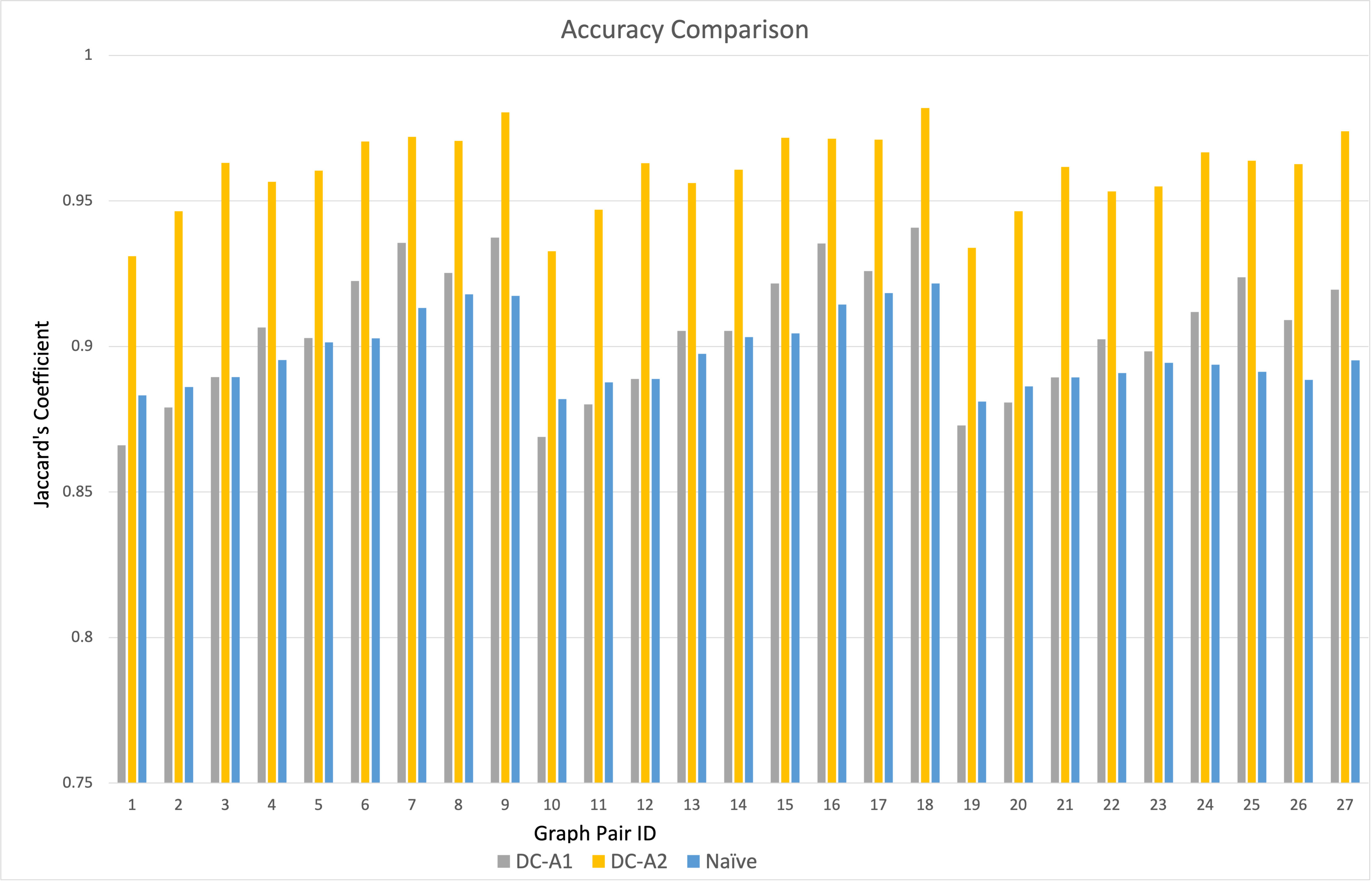
Figure 3: Accuracy Comparison for Synthetic Dataset 1(Refer Table 1).

We use PaRMAT to produce three sets of synthetic data sets for each base graph for experimentation. Our synthetic data set consists of 27 HoMLNs with two layers, each with a different edge distribution. The base graphs start with 100K vertices with 500K edges and go up to 500K vertices and 10 million edges. In the first synthetic data set, both HoMLN layers have power-law degree distribution. In the second synthetic data set, one layer (L1) follows power-law degree distribution and the other one (L2) follows normal degree distribution. In the final synthetic data set, both layers have normal degree distribution.

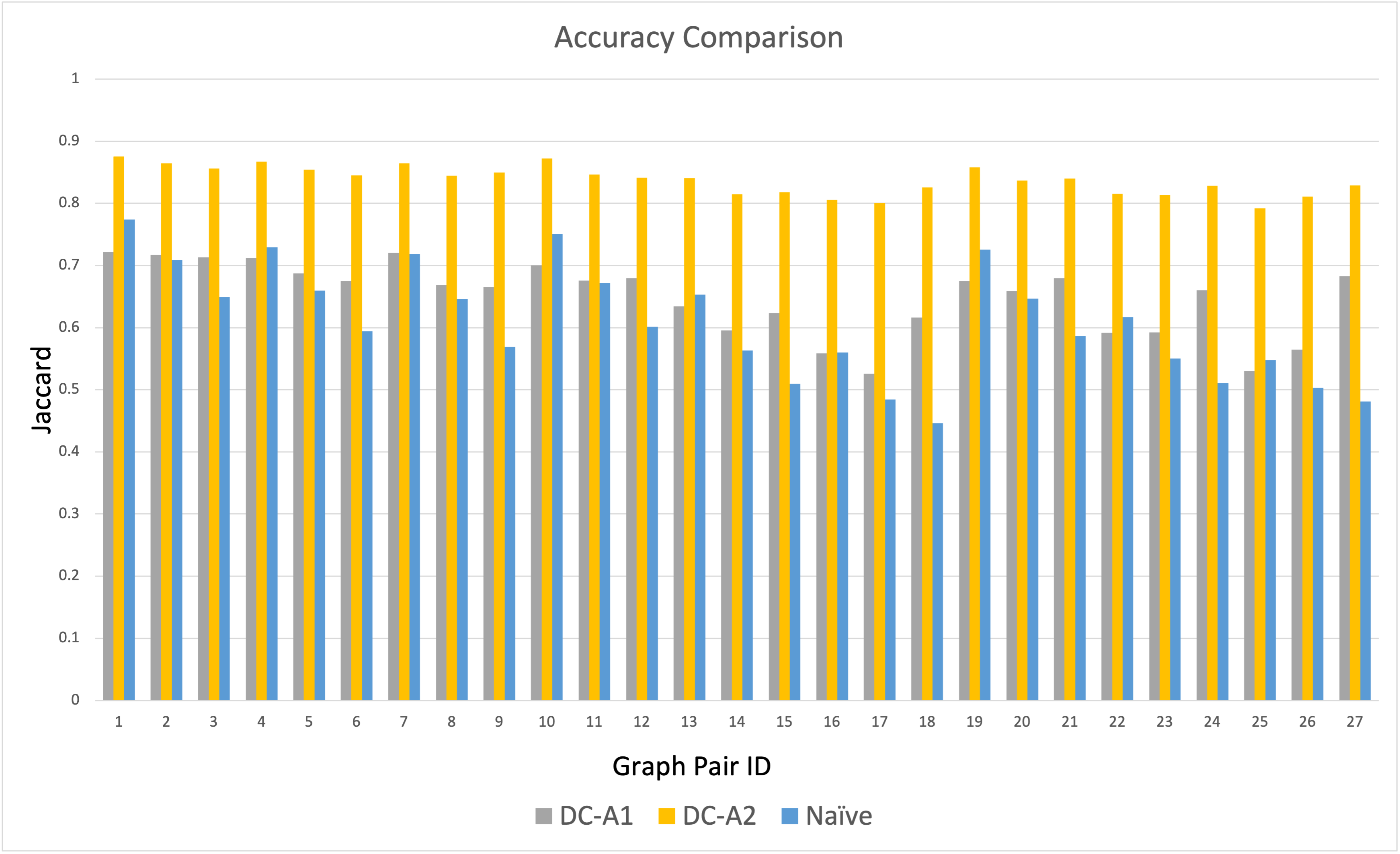
Figure 4: Accuracy Comparison for Synthetic Dataset 2.

For each of the aforementioned data sets, three edge distributions (70, 30; 60, 40; and 50, 50) for a total of 81 HoMLNs with varied edge distributions, number of nodes, and edges are used for experimentation and validation of the proposed heuristics. Table 1 shows the different 2-layer HoMLN used in our data set used in our experiments which are part of the synthetic data set 1. The synthetic data set 1 consists of HoMLN where both the layers have the power-law distribution of edges (L1: Power-law, L2: Power-law). The other two data sets, synthetic data set 2 and 3 have a similar number of nodes and edges in each layer but have (L1: Power-law, L2: Normal) and (L1: Normal, L2: Normal) edge distribution.

Table 3: Accuracy Improvement of DC-A1 and DC-A2 over Naive

Data Set	Degree Distribution	Mean Accuracy
	L1, L2	DC-A1	DC-A2	DC-A1 vs. Naive	DC-A2 vs. Naive
Synthetic-1	Power law, Power law	90.53%	96.01%	+0.86%	+6.96%
Synthetic-2	Power law, Normal	64.90%	83.74%	+6.48%	+37.38%
Synthetic-3	Normal, Normal	76.14%	88.72%	-4.32%	+11.47%
Real world	Power law, Power law	93.11%	98.9%	+10.03%	+10.92%

For our real-world-like data set, the network layers are generated from real-world like monographs using a random number generator. The real-world-like graphs are generated using RMAT with parameters to mimic real-world graph data sets as discussed in [Chakrabarti, 2005]. As a result, the graphs are not single connected components and neither are their ground truth graph.

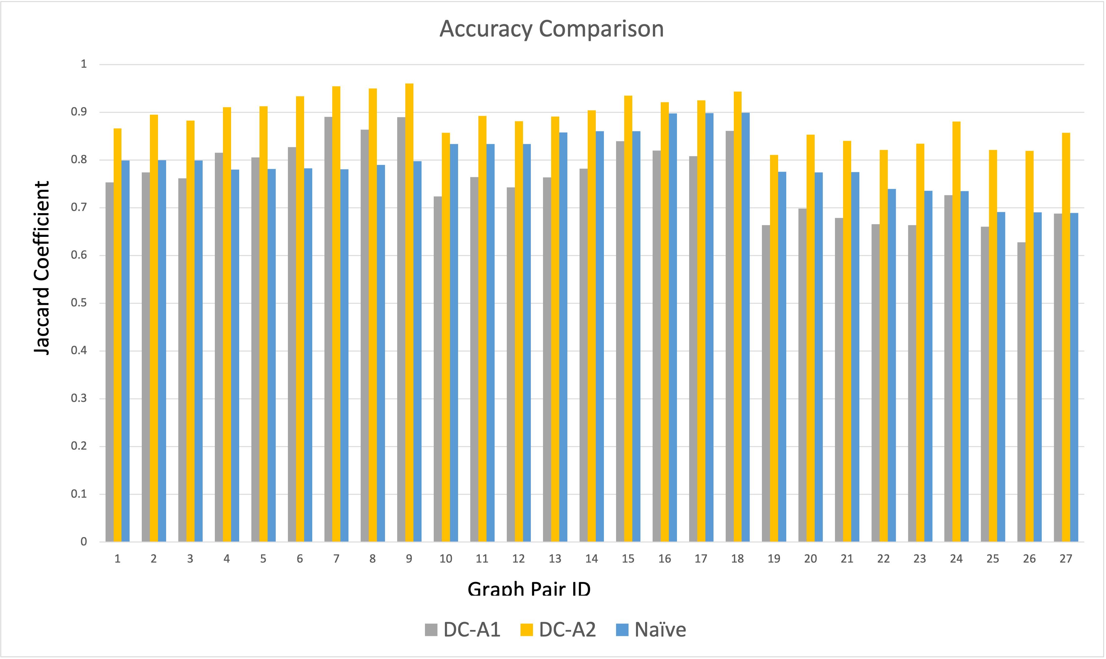
Figure 5: Accuracy Comparison for Synthetic Dataset 3.

7.2 Result Analysis and Discussion

In this section, we present our experimental results. We have tested our proposed heuristics on large real-world and synthetic datasets. As a measure of accuracy, we use the Jaccard coefficient and precision. We compare the execution time of our heuristics against the ground truth execution time as a measure of performance. The Figures 3, 4, and 5 shows the Jaccard coefficient for accuracy of the proposed heuristics-based approaches DC-A1, DC-A2, and the naive approach for the synthetic dataset 1 dataset 2, and dataset 3 respectively. While calculating the Jaccard coefficient, we consider the nodes with equal to or higher than the average degree value in the ground truth as degree hubs. The heuristic DC-A2 performs the best when the accuracy metric is the Jaccard coefficient. It always shows higher accuracy than the naive approach. The heuristic DC-A1 performs better than the naive approach in most cases. Figure 6 shows the Jaccard’s coefficient for the proposed heuristics in real-world dataset [Boldi and Vigna, 2004] [Boldi et al., 2011]. Both heuristics DC-A1 and DC-A2 perform better than the naive approach for all the HoMLN in the dataset. Table 3 shows the mean accuracy and average percentage gain in accuracy for the synthetic and real-world data sets. For all data sets, DC-A2 outperforms the naive approach.

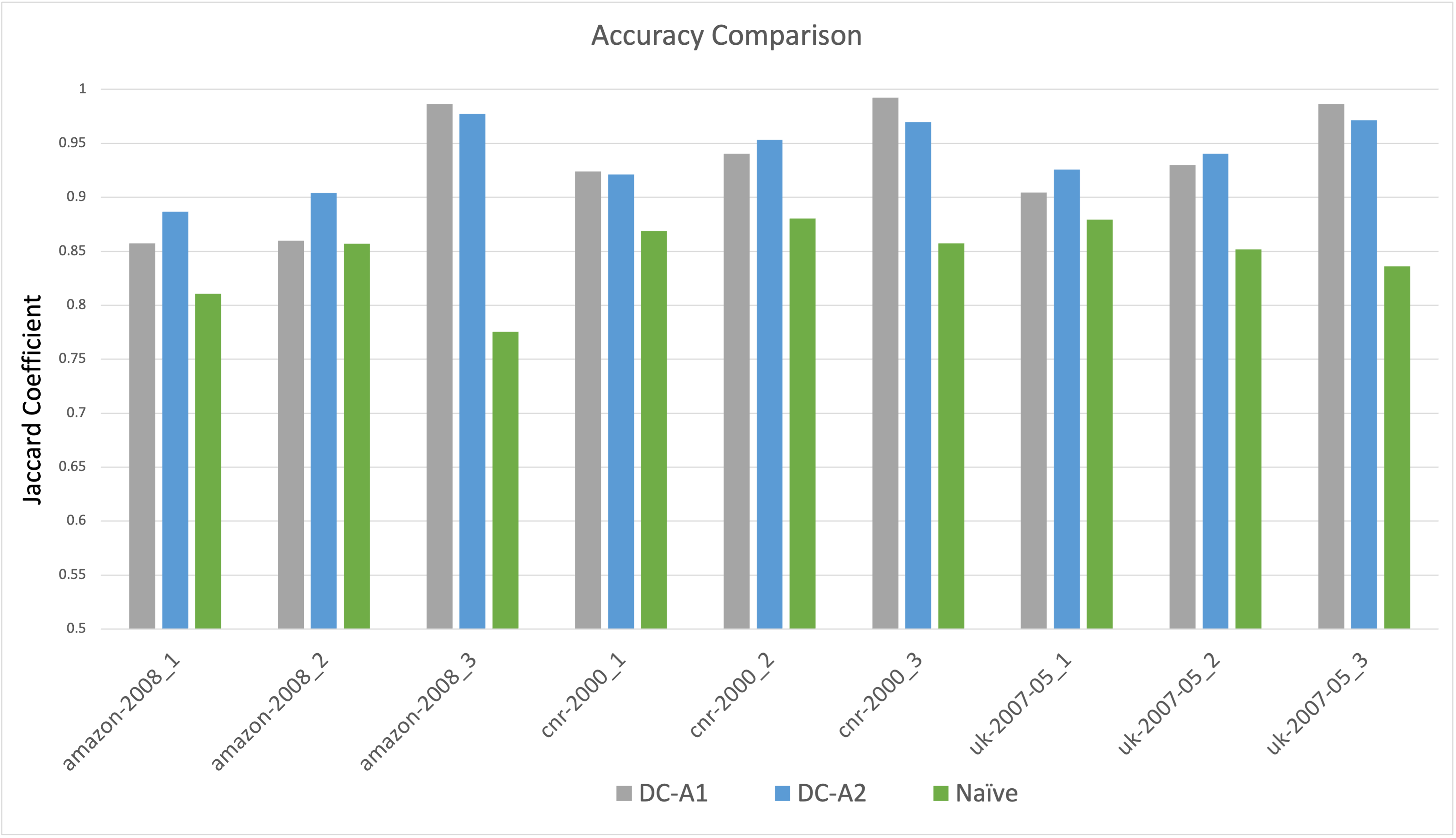
Figure 6: Accuracy Comparison for Real World Dataset(Refer Table 2).

The DC-A1 heuristic performs poorly when both layers have a normal distribution of edges, but performs better than naive in other cases. One reason for the low percentage gain compared to the naive approach is, that for Boolean OR aggregated HoMLN, the naive approach itself has relatively high accuracy.

When precision is used as the measure of accuracy, DC-P1 and DC-P2 outperform DC-A1, DC-A2, as well as the naive approach. For the synthetic data sets, the precision of DC-P1 and DC-P2 is always 100% 7 and more than 96% for the real-world data sets 8.

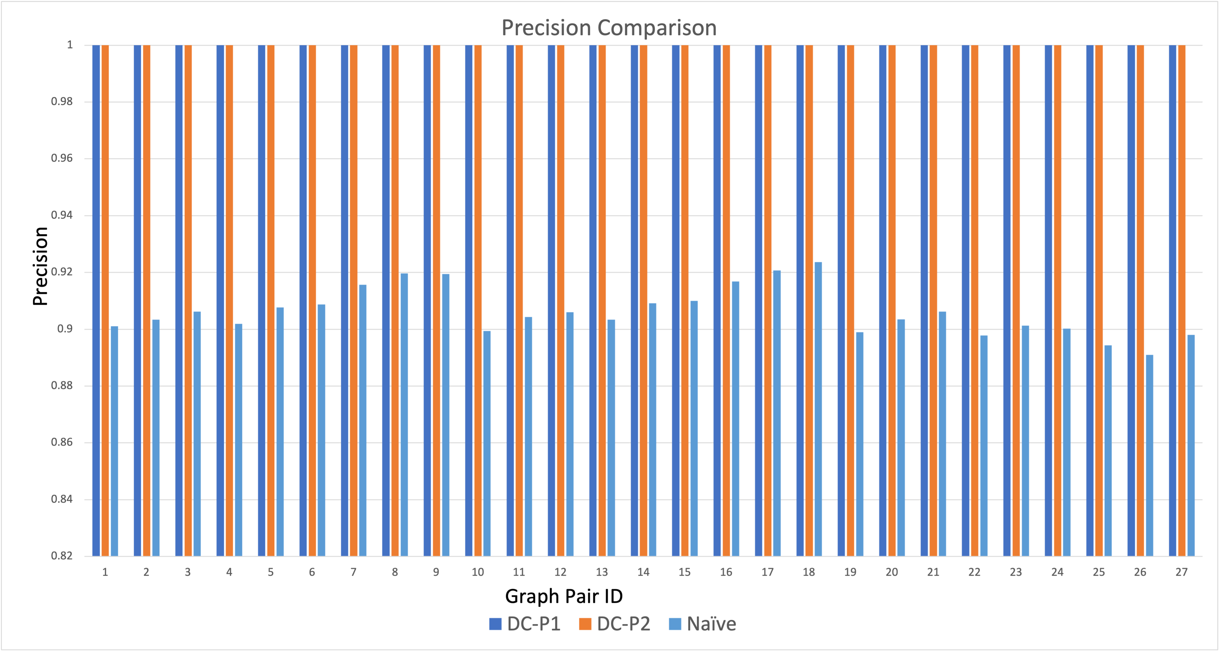
Figure 7: Precision Comparison for Synthetic Dataset 1 (Refer Table 1).

Figure 9 shows the comparison of the execution time of our proposed solutions against the ground truth time for 3 of the largest HoMLN of the synthetic data set 1. The execution time of our approach is calculated as maximum $\Psi$ time of the layers + $\Theta$ time. The ground truth time is computed as time required to aggregate layers into a single graph using Boolean OR function + time required to find the degree hubs of the aggregated graph.

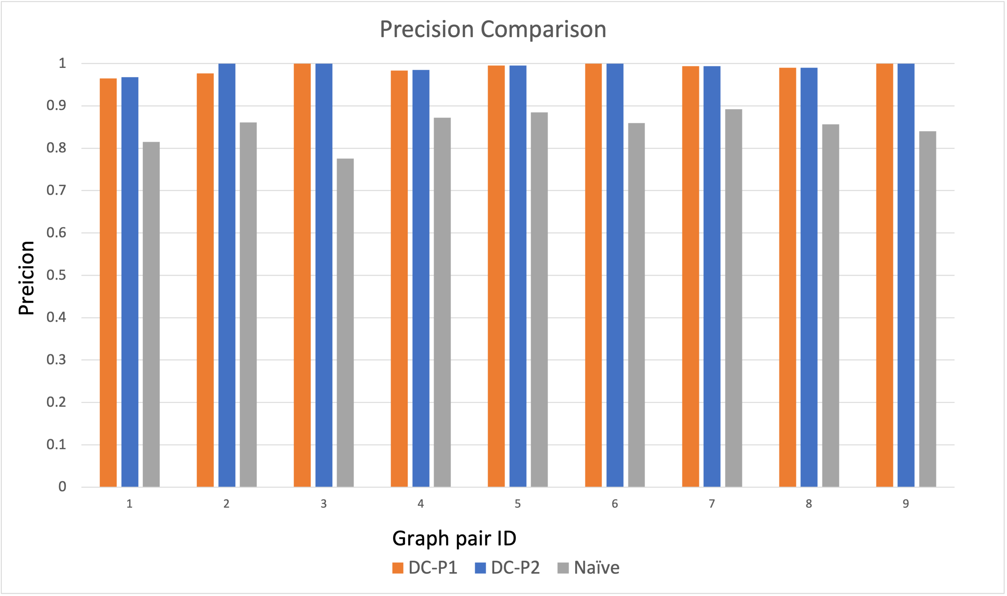
Figure 8: Precision Comparison for real world dataset(Refer Table 2).

As we can see from Figure 9, ground truth execution time is more than an order of magnitude as compared to our proposed approaches in all cases (plotted on log scale).

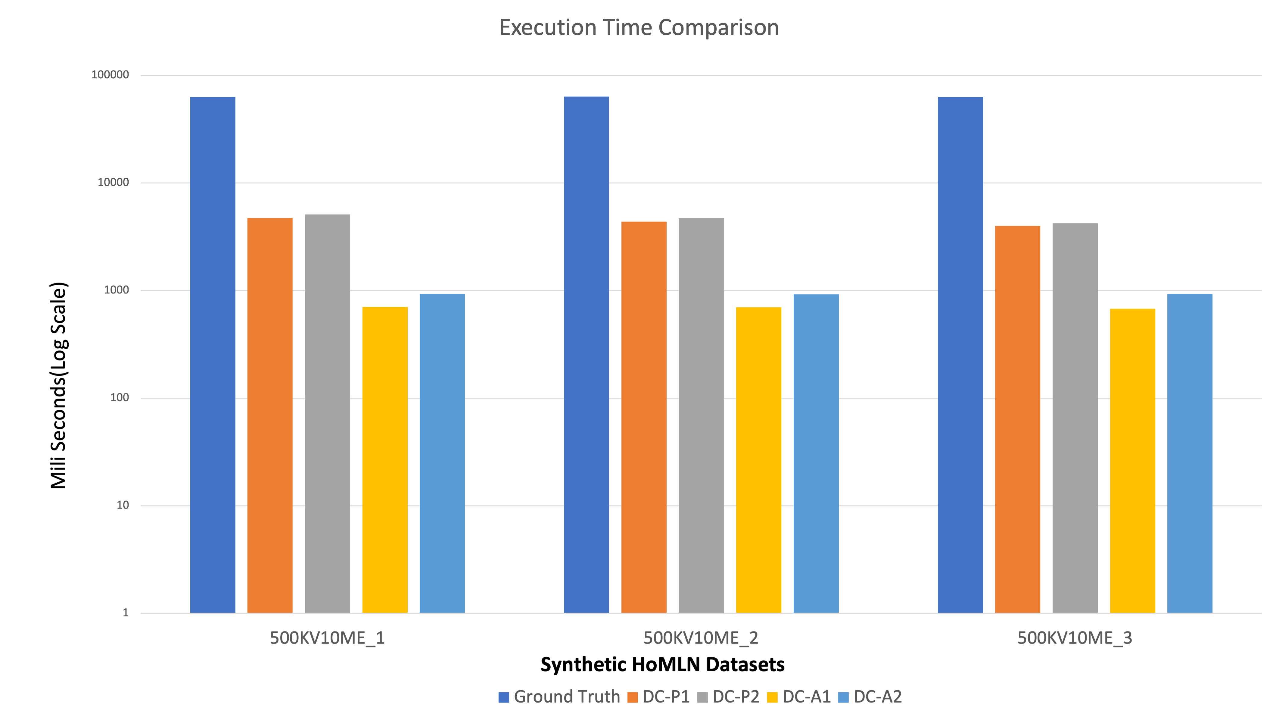
Figure 9: Comparison of Execution Time of the Heuristics against Execution Time of Ground Truth.

As previously mentioned in Section 3, it is a challenge to identify and keep the minimum amount of information required in the network decoupling approach. Theoretically, as more information is kept, the accuracy should go up. For this demonstration, we used a HoMLN consisting of 100K nodes from the synthetic dataset 2 where the first layer follows the power-law distribution and the second layer follows the normal distribution. This HoMLN was taken to minimize any similarity among the layers. The additional information kept is the one-hop neighbors of the nodes in each layer.

In Figure 10 we show that as more information is kept in each layer, the accuracy increases. If no information is kept, we get the lowest accuracy. If we keep one-hop neighbors of all the nodes, we get 100% accuracy.

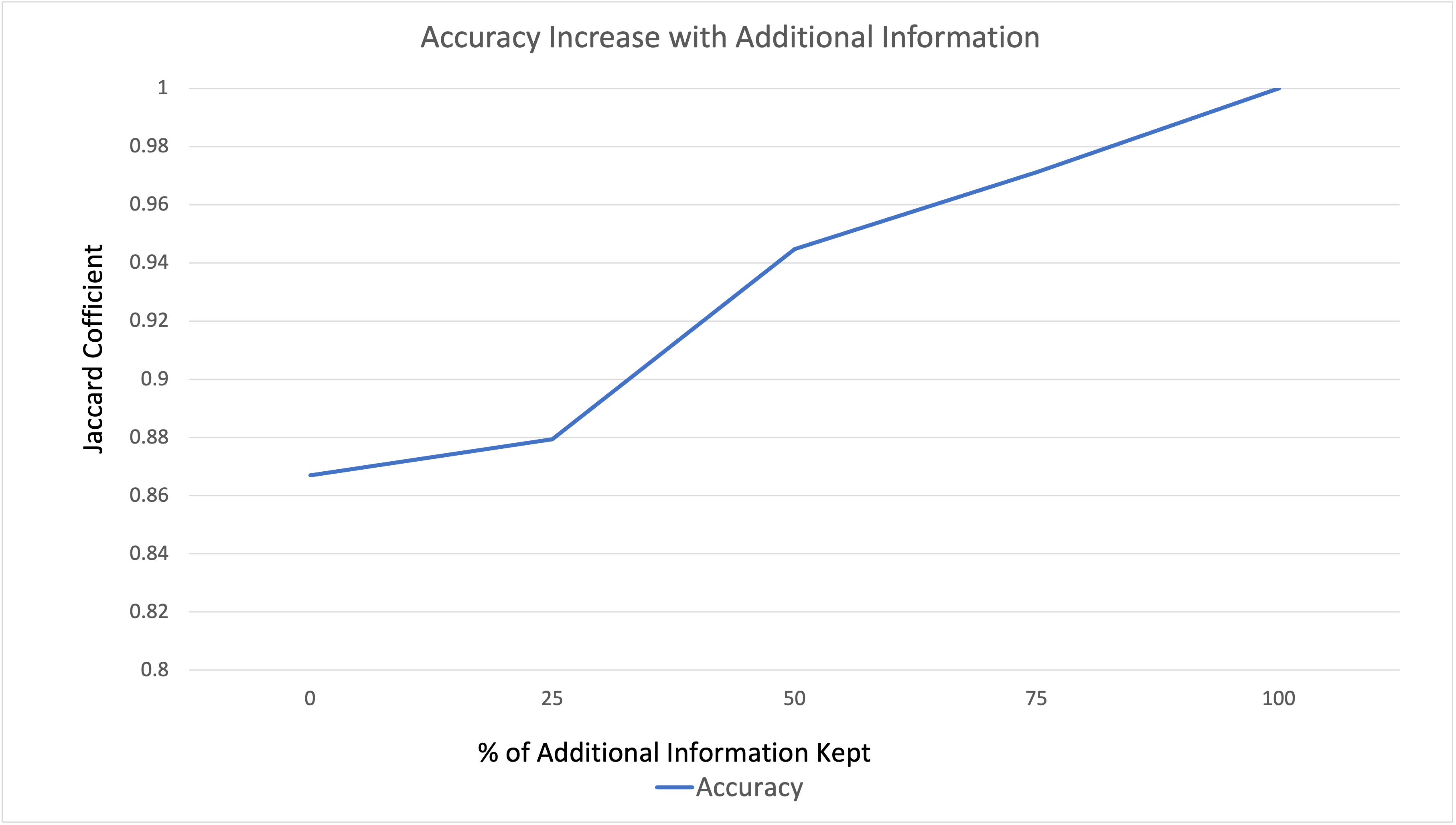
Figure 10: Demonstration of increase in accuracy as more information is kept in each layer for DC-A2.

8 Conclusions and Future Work

In this paper, we proposed several heuristics-based algorithms to compute degree hubs in a HoMLN directly using the decoupling approach. Some of the heuristics (DC-A1 and DC-A2) achieve high accuracy whereas others (DC-P1 and DC-P2) achieve a precision of 1. All proposed algorithms show more than an order of magnitude improvement in efficiency as compared to the traditional aggregation approach used for ground truth. Our hypothesis with respect to more information leading to higher accuracy is also established. Future work includes understanding the cascading effects of accuracy and precision when more layers are used. Also, how to identify and retain additional information that can be used to improve the accuracy of multiple layer centrality computation.

REFERENCES

- dbl, DBLP Data Stats: https://dblp.uni-trier.de/statistics/recordsindblp, Accessed: 24-May-2020.
- Boldi et al., 2011 Boldi, P., Rosa, M., Santini, M., and Vigna, S. (2011). Layered label propagation: A multiresolution coordinate-free ordering for compressing social networks. In Srinivasan, S., Ramamritham, K., Kumar, A., Ravindra, M. P., Bertino, E., and Kumar, R., editors, Proceedings of the 20th international conference on World Wide Web, pages 587–596. ACM Press.
- Boldi and Vigna, 2004 Boldi, P. and Vigna, S. (2004). The WebGraph framework I: Compression techaniques. In Proc. of the Thirteenth International World Wide Web Conference (WWW 2004), pages 595–601, Manhattan, USA. ACM Press.
- Boldi and Vigna, 2014 Boldi, P. and Vigna, S. (2014). Axioms for centrality. Internet Mathematics, 10(3-4):222–262.
- Brandes, 2001 Brandes, U. (2001). A faster algorithm for betweenness centrality. The Journal of Mathematical Sociology, 25(2):163–177.
- Bródka et al., 2011 Bródka, P., Skibicki, K., Kazienko, P., and Musiał, K. (2011). A degree centrality in multi-layered social network. In 2011 International Conference on Computational Aspects of Social Networks (CASoN), pages 237–242.
- Candeloro et al., 2016 Candeloro, L., Savini, L., and Conte, A. (2016). A new weighted degree centrality measure: The application in an animal disease epidemic. PloS one, 11(11):e0165781.
- Chakrabarti, 2005 Chakrabarti, D. (2005). Tools for large graph mining. Carnegie Mellon University.
- Chakrabarti et al., 2004 Chakrabarti, D., Zhan, Y., and Faloutsos, C. (2004). R-mat: A recursive model for graph mining. In Proceedings of the 2004 SIAM International Conference on Data Mining, pages 442–446. SIAM.
- Cohen et al., 2014 Cohen, E., Delling, D., Pajor, T., and Werneck, R. F. (2014). Computing classic closeness centrality, at scale. In Proceedings of the Second ACM Conference on Online Social Networks, COSN ’14, page 37–50, New York, NY, USA. Association for Computing Machinery.
- De Domenico et al., 2013 De Domenico, M., Solé-Ribalta, A., Cozzo, E., Kivelä, M., Moreno, Y., Porter, M. A., Gómez, S., and Arenas, A. (2013). Mathematical formulation of multilayer networks. Physical Review X, 3(4):041022.
- Everett and Borgatti, 1999 Everett, M. G. and Borgatti, S. P. (1999). The centrality of groups and classes. The Journal of mathematical sociology, 23(3):181–201.
- Fortunato and Castellano, 2009 Fortunato, S. and Castellano, C. (2009). Community structure in graphs. In Ency. of Complexity and Systems Science, pages 1141–1163.
- Gaye et al., 2016 Gaye, I., Mendy, G., Ouya, S., Diop, I., and Seck, D. (2016). Multi-diffusion degree centrality measure to maximize the influence spread in the multilayer social networks. In International Conference on e-Infrastructure and e-Services for Developing Countries, pages 53–65. Springer.
- Hagberg et al., 2008 Hagberg, A., Swart, P., and S Chult, D. (2008). Exploring network structure, dynamics, and function using networkx. Technical report, Los Alamos National Lab.(LANL), Los Alamos, NM (United States).
- Khorasani et al., 2015 Khorasani, F., Gupta, R., and Bhuyan, L. N. (2015). Scalable simd-efficient graph processing on gpus. In Proceedings of the 24th International Conference on Parallel Architectures and Compilation Techniques, PACT ’15, pages 39–50.
- Kivelä et al., 2014 Kivelä, M., Arenas, A., Barthelemy, M., Gleeson, J. P., Moreno, Y., and Porter, M. A. (2014). Multilayer networks. Journal of Complex Networks, 2(3):203–271.
- Kretschmer and Kretschmer, 2007 Kretschmer, H. and Kretschmer, T. (2007). A new centrality measure for social network analysis applicable to bibliometric and webometric data. Collnet Journal of Scientometrics and Information Management, 1(1):1–7.
- Liu et al., 2016 Liu, Y., Wei, B., Du, Y., Xiao, F., and Deng, Y. (2016). Identifying influential spreaders by weight degree centrality in complex networks. Chaos, Solitons & Fractals, 86:1–7.
- Pedroche et al., 2016 Pedroche, F., Romance, M., and Criado, R. (2016). A biplex approach to pagerank centrality: From classic to multiplex networks. Chaos: An Interdisciplinary Journal of Nonlinear Science, 26(6):065301.
- Rachman et al., 2013 Rachman, Z. A., Maharani, W., and Adiwijaya (2013). The analysis and implementation of degree centrality in weighted graph in social network analysis. In 2013 International Conference of Information and Communication Technology (ICoICT), pages 72–76.
- Risselada et al., 2016 Risselada, H., Verhoef, P. C., and Bijmolt, T. H. (2016). Indicators of opinion leadership in customer networks: self-reports and degree centrality. Marketing Letters, 27(3):449–460.
- Santra et al., 2017a Santra, A., Bhowmick, S., and Chakravarthy, S. (2017a). Efficient community re-creation in multilayer networks using boolean operations. In International Conference on Computational Science, ICCS 2017, 12-14 June 2017, Zurich, Switzerland, pages 58–67.
- Santra et al., 2017b Santra, A., Bhowmick, S., and Chakravarthy, S. (2017b). Hubify: Efficient estimation of central entities across multiplex layer compositions. In IEEE International Conference on Data Mining Workshops.
- Shi and Zhang, 2011 Shi, Z. and Zhang, B. (2011). Fast network centrality analysis using gpus. BMC Bioinformatics, 12(1).
- Solá et al., 2013 Solá, L., Romance, M., Criado, R., Flores, J., García del Amo, A., and Boccaletti, S. (2013). Eigenvector centrality of nodes in multiplex networks. Chaos: An Interdisciplinary Journal of Nonlinear Science, 23(3):033131.
- Srinivas and Velusamy, 2015 Srinivas, A. and Velusamy, R. L. (2015). Identification of influential nodes from social networks based on enhanced degree centrality measure. In 2015 IEEE International Advance Computing Conference (IACC), pages 1179–1184.
- Tang et al., 2013 Tang, X., Wang, J., Zhong, J., and Pan, Y. (2013). Predicting essential proteins based on weighted degree centrality. IEEE/ACM Transactions on Computational Biology and Bioinformatics, 11(2):407–418.
- Towns et al., 2014 Towns, J., Cockerill, T., Dahan, M., Foster, I., Gaither, K., Grimshaw, A., Hazlewood, V., Lathrop, S., Lifka, D., Peterson, G. D., Roskies, R., Scott, J., and Wilkins-Diehr, N. (2014). Xsede: Accelerating scientific discovery. Computing in Science and Engineering, 16(05):62–74.
- Uddin and Hossain, 2011 Uddin, S. and Hossain, L. (2011). Time scale degree centrality: A time-variant approach to degree centrality measures. In 2011 International Conference on Advances in Social Networks Analysis and Mining, pages 520–524. IEEE.
- Wang et al., 2021 Wang, X., Hu, T., Yang, Q., Jiao, D., Yan, Y., and Liu, L. (2021). Graph-theory based degree centrality combined with machine learning algorithms can predict response to treatment with antiepileptic medications in children with epilepsy. Journal of Clinical Neuroscience, 91:276–282.
- Yang et al., 2014 Yang, Y., Dong, Y., and Chawla, N. V. (2014). Predicting node degree centrality with the node prominence profile. Scientific reports, 4(1):1–7.