Non-asymptotic near optimal algorithms for two sided matchings

Abstract

A two-sided matching system is considered, where servers are assumed to arrive at a fixed rate, while the arrival rate of customers is modulated via a price-control mechanism. We analyse a loss model, wherein customers who are not served immediately upon arrival get blocked, as well as a queueing model, wherein customers wait in a queue until they receive service. The objective is to maximize the platform profit generated from matching servers and customers, subject to quality of service constraints, such as the expected wait time of servers in the loss system model, and the stability of the customer queue in the queuing model. For the loss system, subject to a certain relaxation, we show that the optimal policy has a bang-bang structure. We also derive approximation guarantees for simple pricing policies. For the queueing system, we propose a simple bi-modal matching strategy and show that it achieves near optimal profit.

I Introduction

Two-sided queues, where customers and servers both arrive to a platform/aggregator and then wait to be matched, have been made fairly popular by ride hailing applications like Uber and Lyft that match passengers with drivers, meal delivery couriers like Grubhub and DoorDash that match diners with delivery couriers, and crowdsourcing platforms like Amazon MTurk, where tasks are matched to workers/volunteers. The objective of the platform is to maximize profit, while improving the market efficiency.

To earn revenue, the platform sets a two sided or one sided price. With two sided pricing, both the customers and the servers are advertised a (possibly different) price, and customers willing to pay the quoted price and servers who are willing to serve for the quoted price enter the system. The platform profit is then the difference between the two prices. In a one sided price model, only the customers are quoted a price, and customers who are willing to pay enter the system. The server arrival rate is assumed to be fixed, and insensitive to price. In this model, the platform keeps a fraction of the revenue (made from customers) to itself and distributes the rest uniformly across all servers. In many practical systems, server payoffs are better modelled as long-term rewards [1], and thus considering one sided pricing is reasonable. In both models, the price is dynamically adjusted to maximize profit, and to efficiently match supply and demand.

With two-sided queues, we consider two well studied models: the loss model, and the queueing model. For both models, we assume one sided pricing, where the platform advertises a state dependent price that determines the rate of arrival of customers, while the rate of arrival of servers is fixed and insensitive to the platform price.

Under the loss model, servers arrive into a queue and wait, while arriving customers are instantaneously matched to the head of the line server, if any. A customer arriving when no servers are present is lost. The objective we consider with the loss model is to maximize a linear combination of the platform’s profit and the expected delay experienced by servers, and the goal is to find the optimal dynamic price to maximize this objective function.

With the queuing model, both the servers and the customers wait in their respective queues, and are matched appropriately. In this case, we consider the objective of maximizing the platform’s profit subject to the stability of the customer queue. The goal is to design a dynamic pricing and matching strategy to achieve optimal platform profit while ensuring the stability of the customer queue.

Prior Work: With a single sided queue (where server is fixed and only customers arrive), [2] considered a loss-system with finite resource capacity. A customer arriving when all resources are occupied is lost, and the problem is to decide the price of admission given the state of the system at each time to maximize the expected payoff. Similar pricing models have been considered for a queuing system, where customers wait in a queue, and server’s service distribution is exponential with a tuneable parameter. Optimal admission control, with and without pricing, and service parameter selection, so as to maximize a linear combination of expected payoff and expected waiting time has been considered in [3, 4, 5, 6, 7, 8], assuming Poisson arrivals. In particular, [6] exactly characterizes the optimal policy, though not in closed-form, while [8] derives an asymptotically optimal dynamic pricing policy.

Two sided queues have been considered in [1, 9, 10, 11, 12, 13, 14, 15], where both customers and servers arrive over time, and wait to be matched. In particular, most of these papers are motivated from ride-hailing applications such as Uber, Lyft, or meal delivery services Grubhub, DoorDash, etc. Some of the results [13, 1, 14, 15] in this area focus on the importance of dynamic pricing over static pricing. Under a suitable fluid scaled limit of this system, [1] showed that static pricing is sufficient to optimize the objective function, and dynamic pricing only helps in improving the robustness of the system.

An extension of this two-sided queue model with multiple types of servers and customers has also been considered in [16, 17, 18, 19, 10], where an additional bipartite matching decision has to be made. In [16], limiting results of matching rates between certain customer and server types with FCFS scheduling have been analyzed. Without pricing, the optimal matching to minimize the queueing cost has been analyzed in [18] under a suitably scaled large system limit. With the objective of minimizing the discounted reward obtained by matching customers and servers over a finite horizon, while accounting for the waiting costs, [19] analyzed fixed pricing strategies, while dynamic pricing strategies were considered in [20, 10]. Most of these analyses are presented using a large system scaling regime.

To summarize, in prior work, either exactly optimal but non-closed form policies have been characterized, or structural properties of the optimal policy have been established, or performance analysis of simple strategies has been performed. Importantly, to the best of our knowledge, any analysis of an explicit policy has been via an asymptotic (large system) scaling.

Our Contributions: Compared to prior work, the focus of this work is to consider simple (one-sided) pricing strategies for two-sided queues without considering any large system limits, e.g., fluid limits or asymptotics, with near-optimal performance. Specifically, we model server arrivals as an exogenous random process (independent of the system state and the matching/pricing policy). On the other hand, customer arrivals are modulated by the price $p$ posted by the platform. Formally, we model the customer arrival rate $\mu(p)$ as a non-increasing concave function of the platform price $p$. We consider two variants of our model: a loss model where customers not served upon arrival are blocked, and a queueing model, where customers wait in a FCFS queue until they are matched with a server. Our contributions for these two models are as follows.

I-1 Loss System

For the loss system, we consider that the customer and server arrival processes are Poisson, and the objective is to maximize a linear combination of the platform’s profit and the expected delay experienced by servers.

When function $\mu(p)$ is linear in $p$ (which is an important case [21] in pricing/profit models), we consider a suitable relaxation of the objective, for which we show that the optimal pricing strategy has a simple bang-bang style threshold structure. This means that the price is set to be the maximum feasible value when the number of servers is less than a threshold, and to the minimum feasible value when the number of servers exceeds the same threshold. This bang-bang structure of the optimal policy implies that computing the optimal policy boils down to a simple one-dimensional search. Moreover, the same structure can also be exploited to speed up online learning of the optimal policy via reinforcement learning (see [22]). While the relaxation we consider is quite similar to models studied in the literature, that a linear price sensitivity function admits such a simple optimal policy has not been observed before, to the best of our knowledge. Additionally, we show that a simple static pricing model can be near-optimal under certain conditions. Specifically, we derive universal upper bounds on the objective value attainable by any policy, and show that static pricing can achieve a performance that is ‘close’ to the upper bounds in many cases.

I-2 Queueing System

Compared to the loss system, with the queueing system, we consider general customer and server arrival distributions, and a discrete time setup. The objective function is to maximize the platform’s profit subject to the customer queue being stable. Towards that end, we propose an algorithm that charges a static price, and uses a bi-modal matching strategy with a single threshold $U$, to decide the number of customer-server pairs that should be matched at each time slot. The main idea of the algorithm is to choose a static price thereby making the customer arrival rate constant over time. The threshold $U$ is chosen in such way that the rate of customer departures (number of customer-server matched pairs) in each time slot is close to the revenue-optimal departure rate. Small perturbations in the departure rate, required to maintain the customer queue at a steady level, result in near-optimal performance.

In particular, we show that the proposed strategy has an additive sub-optimality gap of $O\left(\frac{\log U}{U}\right)$. Moreover, the expected delay experienced by customers with the proposed strategy is $O(U)$. Thus, even though we do not explicitly include the expected delay experienced by the customers in the objective function and only enforce the constraint that the customer queue should be stable, a by-product of the proposed algorithm and its analysis is that the expected delay experienced by the customers is also controlled by the threshold $U.$ Thus, given additional QoS constraints on the expected delay experienced by the customers, we can choose the threshold $U$ to achieve a tradeoff between the sub-optimality gap and the expected delay.

II Loss model

In this section, we consider the case where customers do not wait, i.e., customers that arrive when there are no servers in the system get lost/blocked.

II-A Model and Preliminaries

We model the loss system in continuous time. Servers arrive to the platform as per a Poisson process with rate $\lambda.$ Upon arrival, servers wait in an infinite buffer queue, until they are matched to a customer. The customer arrival rate $\mu=g(p)$ is a function of the platform’s posted price $p,$ where $g$ is a strictly decreasing and concave function of $p.$ Specifically, when the platform posts price $p,$ the time until the next customer arrival is assumed to be exponentially distributed with mean $1/g(p).$ Thus, the function $g$ captures the price sensitivity of the customer base.

We assume that the price $p$ is constrained to lie in $[p_{\min},p_{\max}],$ where $0<p_{\min}<p_{\max},$ and that the price defaults to $p_{\max}$ when there are no servers available. Customers that arrive when there are no servers are blocked/lost, i.e., customers do not queue.

Under the above model, given the memorylessness in server and customer interarrival times, the state of the system is captured by the number of servers in the queue. Denoting the platform’s price when there are $i$ servers in the queue by $p_{i},$ the state evolves as per the (controlled) birth-death Markov chain depicted in Figure 1. Here, $\mu_{i}:=g(p_{i})$ and $\mu_{i}\in[g(p_{\max}),g(p_{\min})].$

Figure 1: Birth death chain for server evolution

The goal of the platform is to set prices $(p_{i},\ i\in\mathbb{N})$ so as to maximize $\tilde{C}=\lambda E\left[P\right]-\tilde{w}E\left[N\right],$ where $P$ denotes the stationary price seen by a (matched) customer, $N$ denotes the stationary number of servers in the system, and $\tilde{w}$ is a positive weight. The impicit constraint here is of course that the server queue is stable, i.e., the Markov chain describing the temporal evolution of the number of waiting servers is positive recurrent. The first term in $\tilde{C}$ is the revenue rate for the platform, the second may be interpreted as the (holding) cost associated with servers idling. By Little’s law, maximizing $\tilde{C}$ is equivalent to maximizing

$$C=\frac{\tilde{C}}{\lambda}=E\left[P\right]-\tilde{w}E\left[T\right]=E\left[P\right]-wE\left[N\right]$$

where $T$ denotes the stationary server sojourn time, $w=\frac{\tilde{w}}{\lambda}.$

The optimal policy can be computed numerically using standard machinery from the theory of Markov decision process (see, for example, [23]). Related problem formulations are also analysed in [2, 6]; these references characterize structural properties of the optimal policy. However, our goal here is to consider a relaxed version of the above objective, which admits a more explicit analysis.

We now describe our relaxed objective. For a given policy $(p_{i},\ i\in\mathbb{N}),$ let the stationary distribution associated with the server occupancy be denoted by $\pi=(\pi_{i},\ i\in\mathbb{N}).$ Our objective $C$ may be expressed in terms of $\pi$ as follows:

$$C =\underbrace{\sum_{i=1}^{\infty}\pi_{i-1}p_{i}}_{E\left[P\right]}-w\underbrace{\sum_{i=1}^{\infty}i\pi_{i}}_{E\left[N\right]}.$$

It is important to note that in the expression for $E\left[P\right],$ we have $\pi_{i-1}$ multiplying $p_{i}$ because the long run fraction of (server) departures out of state $i$ (i.e., departures that leave behind $i-1$ servers in the system) equals the long run fraction of server arrivals that see $i-1$ servers in the system, which, by PASTA, equals $\pi_{i-1}.$ Our relaxed objective is now stated as follows.

$$C_{\text{rel}} =\sum_{i=1}^{\infty}\pi_{i-1}p_{i-1}-w\sum_{i=1}^{\infty}i\pi_{i}=\sum_{i=0}^{\infty}\pi_{i}p_{i}-w\sum_{i=1}^{\infty}i\pi_{i}$$ (1)

Note that under this relaxation, the term $\sum_{i=1}^{\infty}\pi_{i-1}p_{i}$ in the objective is replaced by the more tractable term $\sum_{i=1}^{\infty}\pi_{i-1}p_{i-1}.$ The motivation for this relaxation is of course to align the distribution used to average price with the stationary distribution. Clearly, $C_{\text{rel}}$ and $C$ would be close when the price varies slowly with state. Specifically, for static pricing policies, the two objectives are identical. However, even for the bang-bang type policies we consider later, we find that two objectives are aligned, as we demonstrate as part of our numerical experiments in Section II-E.

Most of our results will be derived for the case where the price sensitivity function $g$ is linear:

Assumption 1.

$g(p)$ depends linearly on $p,$ i.e., $g(p)=\beta-\alpha p,$ where $\beta,\alpha>0.$ Moreover, $\mu_{\max}:=\beta-\alpha p_{\min}>\lambda,$ and $\mu_{\min}:=\beta-\alpha p_{\max}>0.$

We also consider a more general class of concave price sensitivity functions, and prove bounds on the sub-optimality of simple static pricing policies for this class.

Assumption 2.

$g(p)=(\beta-\alpha p)^{\theta},$ where $\theta\in(0,1],$ and $\beta,\alpha>0.$ Moreover, $\mu_{\max}:=(\beta-\alpha p_{\min})^{\theta}>\lambda,$ and $\mu_{\min}:=(\beta-\alpha p_{\max})^{\theta}>0.$

Under both assumptions, note that $p_{\max}<\frac{\beta}{\alpha}.$ Thus, $\frac{\beta}{\alpha}$ is a trivial upper bound on the objective value achievable. More refined bounds will be derived in Section II-D.

II-B Linear price sensitivity & relaxed objective: Optimal policy

Throughout this section, we make Assumption 1, and consider the relaxed objective $C_{\text{rel}}$ (see (1)). Recall that the number of servers evolves as per the birth death Markov chain shown in Figure 1. Here, $p_{i},$ or equivalently $\mu_{i}=g(p_{i}),$ can be interpreted as the ‘action’ taken in state $i.$ Recall also that $p_{0}=p_{\max};$ let $\mu_{0}:=g(p_{0})=\mu_{\min}.$

We begin by rewriting $C_{\text{rel}}$ as follows.

Lemma 1.

Under Assumption 1, $C_{\text{rel}}=\frac{1}{\alpha}\left(\beta-\pi_{0}\mu_{0}-\lambda\right)-w\sum_{i=1}^{\infty}i\pi_{i}.$

Lemma 1 states that under linear price sensivity, the first term in the relaxed objective decreases linearly in $\pi_{0}.$ In other words, maximizing the first term boils down to minimizing $\pi_{0}.$ We now exploit this property to show that the optimal policy is of bang-bang type.

Theorem 3.

Under Assumption 1 (wherein the price sensitivity function $g$ is linear), there exists a policy that optimizes $C_{\text{rel}}$ of the form

$$p_{i}=\left\{\begin{array}[]{cl}p_{\max}&\text{ for }i<\ell^{*}\\ p^{*}&\text{ for }i=\ell^{*}\\ p_{\min}&\text{ for }i>\ell^{*}\end{array}\right.,$$

where $\ell^{*}\in\mathbb{N}\cup\{\infty\},$ $p^{*}\in[p_{\min},p_{\max}].$

The bang-bang policy stated in Theorem 3 has the following interpretation: When there are fewer than $\ell^{*}$ servers in the system, the platform sets the maximum price, thereby limiting customer arrivals as far as possible so as to provide the maximum upward drift to the server queue. On the other hand, when the number of servers exceeds $\ell^{*},$ the platform sets the minimum price, thereby maximizing the rate of customer arrivals and providing the maximum downward drift to the server queue. Finally, when there are exactly $\ell^{*}$ servers, the platform sets an intermediate price $p^{*}.$ Thus, the platform in effect seeks to maintain the number of servers at around $\ell^{*}$ to the extent that its control over customer arrivals permits. As will be apparent from the proof of Theorem 3, the aforementioned policy effectively minimizes the probability that the server queue becomes empty, subject to an upper bound on the expected stationary number of servers in the system.

Remark 4.

It is important to note that the bang-bang structure of the optimal policy as stated in Theorem 3 is significantly stronger than the monotonicity properties that are typically established in structured MDPs (see, for example, [24]). Moreover, note that Theorem 3 is proved using the representation of the relaxed objective in Lemma 1, which in turn relies heavily on the linearily of the price sensitivity function $g.$

Remark 5.

While the optimal policy as stated in Theorem 3 is parameterized by $(\ell^{*},p^{*}),$ it can also be parameterized via a single parameter $x^{*}\in\mathbb{R}_{+}.$ The two parameterizations are related as follows: $\ell^{*}=\left\lceil x^{*}\right\rceil,$ and $p^{*}=p_{\max}-(\left\lceil x^{*}\right\rceil-x^{*})(p_{\max}-p_{\min}).$ This one-dimensional parameterization simplifies the task of computing the optimal policy as a function of the system parameters, and is amenable to efficient online learning via standard stochastic approximation techniques (see [22]).

Proof of Theorem 3.

It suffices to show that an optimal policy of the specified form exists for any constrained optimization of the following form, parameterized by $\mathcal{C}>0.$

$$\max\ \frac{1}{\alpha}\left(\beta-\pi_{0}\mu_{0}-\lambda\right)\qquad s.t.\ \sum_{i=1}^{\infty}i\pi_{i}\leq\mathcal{C}$$

Equivalently, it suffices to show that an optimal policy of the specified form exists for any constrained optimization of the following form:

$$\min\ \pi_{0}\qquad s.t.\ \sum_{i=1}^{\infty}i\pi_{i}\leq\mathcal{C}$$ (2)

That this problem, which is well motivated in its own right, has an optimal solution of the bang-bang form specified, is proved as Lemma 2. ∎

The optimization (2) is a natural and well-motivated problem in the context of controlled birth death Markov chains over $\mathbb{Z}_{+}$, where the goal is to minimize the stationary probability of state 0, subject to an upper bound on the expectation of the steady state distribution. Since this problem is interesting in its own right, we study it (independently of its application to our dynamic pricing model) in the following section.

II-C A bang-bang lemma for controlled Markov chains

Consider a birth death Markov chain over state space $\mathbb{Z}_{+}.$ The transition rate from state $i$ to $i+1$ is denoted by $\lambda_{i}$ for $i\geq 0$ and the transition rate from state $i$ to $i-1$ is denoted by $\mu_{i}$ for $i\geq 1.$ For $i\geq 1$ $\rho_{i}:=\frac{\lambda_{i-1}}{\mu_{i}}.$

Assuming the chain is positive recurrent, the stationary distribution is given by $\pi_{i}=\frac{h_{i}}{\sum_{j=0}^{\infty}h_{j}},$ where $h_{0}=1,$ $h_{i}=\prod_{j=1}^{i}\rho_{j}$ for $i\geq 1.$

With $\rho_{i}$ constrained to lie in $[\underline{\rho},\bar{\rho}],$ where $0<\underline{\rho}<\bar{\rho},$ our goal is to minimize $\pi_{0}$ subject to a moment condition on the stationary distribution. Formally, this is posed as:

$$\begin{array}[]{rl}\min.&\pi_{0}\\ s.t.&\sum_{i=0}^{\infty}i\pi_{i}\leq C\\ &\rho_{i}\in[\underline{\rho},\bar{\rho}]\quad(i\geq 1)\end{array}$$ (3)

An implicit constraint here is of course that the chain is positive recurrent. Clearly, $\underline{\rho}<1$ is necessary and sufficient for the feasibility of positive recurrence of the chain. Note also that if $\underline{\rho}<1$ and $\frac{\underline{\rho}}{1-\underline{\rho}}>C,$ then the optimization (3) is infeasible (since the expected steady state value of the chain is easily seen to be at least $\frac{\underline{\rho}}{1-\underline{\rho}}$). Thus, the optimization (3) is well posed if $\underline{\rho}<1$ and $\frac{\underline{\rho}}{1-\underline{\rho}}\leq C.$ Under these conditions, the following lemma shows that the optimal control is of bang-bang type.

Lemma 2.

Assuming $\underline{\rho}<1$ and $\frac{\underline{\rho}}{1-\underline{\rho}}\leq C,$ the optimal solution of (3) is of the form

$$\rho_{i}=\left\{\begin{array}[]{cl}\bar{\rho}&\text{ for }i<\ell^{*}\\ r^{*}&\text{ for }i=\ell^{*}\\ \underline{\rho}&\text{ for }i>\ell^{*}\end{array}\right.,$$

where $\ell^{*}\in\mathbb{N}\cup\{\infty\},$ $r^{*}\in[\underline{\rho},\bar{\rho}].$

This lemma is proved by showing that any feasible policy that does not have the above bang bang structure can be improved upon via a perturbation towards this structure (details can be found in [25]). The proof arguments are similar to those in [26], where a bang-bang style policy is shown to be optimal in a different context.

II-D Single (static) price policies

Next, we consider the simplest pricing policy: a constant, state-independent price, under the relaxed objective $C_{\text{rel}}.$ While static pricing might seem naive, we show that under certain conditions, if the static price is chosen carefully, the suboptimality relative to the (unknown) optimal policy can be bounded. This is somewhat analogous to what happens with the classical server speed scaling problem, where it is known that a suitably chosen static speed choice is constant competitive under a stochastic workload model [27, 28].

We begin by deriving some universal upper bounds on the objective value under any policy (not necessarily static).

II-D1 Universal upper bounds

Lemma 3.

Under Assumption 2, for any policy, we have $C_{\text{rel}}\leq g^{-1}(\lambda).$

Lemma 4 (Light traffic bound).

Under Assumption 2, for any policy, $C_{\text{rel}}\leq\max_{p\in[p_{\min},p_{\max}]}\left(p-\frac{\tilde{w}}{g(p)}\right).$

Next, we apply these upper bounds to study the competitiveness of static pricing for the case of linear price sensitivity.

II-D2 Competitiveness under linear model

We begin by specializing the above universal bounds to Assumption 1, i.e., $g(p)=\beta-\alpha p,$ where $\beta,\alpha>0.$ An application of Lemma 3 for this case yields: $C_{\text{rel}}\leq\frac{\beta-\lambda}{\alpha}.$ Next, application of Lemma 4 yields: $C_{\text{rel}}\leq\max_{p\in\mathbb{R}}\left(p-\frac{\tilde{w}}{\beta-\alpha p}\right)=\frac{\beta-2\sqrt{\tilde{w}\alpha}}{\alpha}.$ Combining the two bounds above together, under Assumption 1, for any policy,

$$C_{\text{rel}}\leq\frac{\beta}{\alpha}-\max\left(\frac{\lambda}{\alpha},\frac{2\sqrt{\tilde{w}\alpha}}{\alpha}\right).$$ (4)

Clearly, the condition $\beta>2\sqrt{\tilde{w}\alpha}$ is a necessary condition for positive objective value under any policy. Now the optimal static price is given by $p^{*}=\operatorname*{arg\,max}_{p\in[p_{\min},p_{\max}]}\left(p-\frac{\tilde{w}}{\beta-\alpha p-\lambda}\right).$ If $\mu_{\max}=\beta-\alpha p_{\min}\geq\lambda+\sqrt{\alpha\tilde{w}},$ then $p^{*}=\frac{\beta-\sqrt{\alpha\tilde{w}}-\lambda}{\alpha}.$ The static policy that always chooses the price $p^{*}$ would then have payoff

$$C_{\text{rel}}(p^{*})=\frac{\beta-2\sqrt{\alpha\tilde{w}}-\lambda}{\alpha}.$$ (5)

Comparing (4) and (5), it follows that so long as $\mu_{\max}\geq\lambda+\sqrt{\alpha\tilde{w}},$ i.e., it is feasible to maintain a $\sqrt{\alpha\tilde{w}}$ slack in the customer arrival rate relative to the server arrival rate, the reduction in payoff from $\frac{\beta}{\alpha}$ under the optimal static pricing policy is at most twice that under any policy. Reframing the objective as a minimization of the payoff reduction from its (unattainable) upper bound $\frac{\beta}{\alpha},$ this implies a competitive ratio of at most two.

II-D3 Competitiveness under non-linear model

We now consider the more general concave price sensitivity model specified by Assumption 2. Specializing our two upper bounds to this particular choice of $g(\cdot),$ we get that under any policy,

$$C_{\text{rel}}\leq\frac{\beta}{\alpha}-\max\left(\frac{\lambda^{1/\theta}}{\alpha},\frac{B}{\alpha}\right),$$ (6)

where $B:=(\tilde{w}\alpha\theta)^{1/(\theta+1)}(1+1/\theta).$

Unlike in the linear case however, this non-linear model for $g(\cdot)$ does not admit a closed form characterization of the optimal static price. We thus consider two separate cases based on which term contributes to the max in (6). For each of these cases, a different reasonable choice of static price is considered.

Case 1 (heavy traffic): $\lambda^{1/\theta}\geq B$

Consider the static policy that sets the price $p$ such that $\mu=(\beta-\alpha p)^{\theta}=\gamma\lambda,$ where $\gamma>1.$ Clearly, such a $\gamma$ exists, given that $\mu_{\max}>\lambda.$ The payoff under this policy is

$$C_{\text{rel}} =\frac{\beta}{\alpha}-\frac{(\gamma\lambda)^{1/\theta}}{\alpha}-\frac{w}{(\gamma-1)\lambda}.$$

For large $\lambda,$ the last term above would be negligible, meaning the payoff reduction from $\frac{\beta}{\alpha}$ would be (approximately) at most a factor of $\gamma^{1/\theta}$ of that under any policy.

Case 2 (light traffic): $\lambda^{1/\theta}<B$

In this case, consider the static policy that sets the price such that $\mu=(\beta-\alpha p)^{\theta}=\gamma B^{\theta},$ where $\gamma>1.$ Such a choice is of course feasible only when $\mu_{\max}>B^{\theta}.$ If so, the cost under this policy is bounded as:

$$C_{\text{rel}} \geq\frac{\beta}{\alpha}-\frac{\gamma^{1/\theta}B}{\alpha}-\frac{w}{(\gamma-1)B^{\theta}}.$$

For large $B,$ the last term above would be negligible, meaning the payoff reduction from $\frac{\beta}{\alpha}$ would be (approximately) at most a factor of $\gamma^{1/\theta}$ of that under any policy, as before.

II-E Numerical experiments

Since we have used the relaxed objective $C_{\text{rel}}$ in the preceding sections, we now present some numerical results illustrating the connection between $C_{\text{rel}}$ and $C.$ Specifically, we compare both objectives over the (one-dimensional) space of bang-bang policies of the kind we proved as optimal for $C_{\text{rel}}$ for linear price sensitivity.

In Figure 2, we plot $C_{\text{rel}}$ and $C$ as a function of a single parameter $x$ that specifies the bang bang policy, as described in Section II-B, for different values of $w.$ We note that increasing the weight $w$ on the holding cost decreases the objective values, and decreases the optimal choice of $x,$ as expected. However, what is interesting to note is that the optimal choice of $x$ under the relaxed objective matches almost perfectly with the optimal choice under the original objective. This suggests that the optimal bang-bang policy under the relaxed objective is also a near optimal choice (within the class of bang-bang policies) for our original objective.

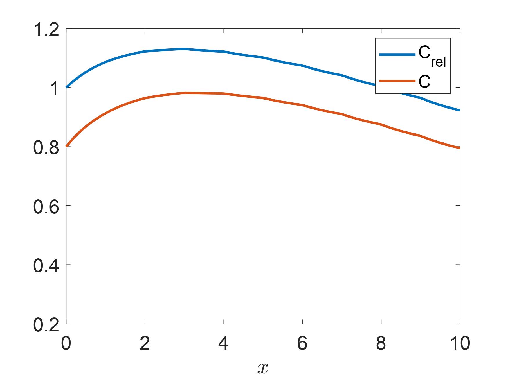
(a) $w=0.05$

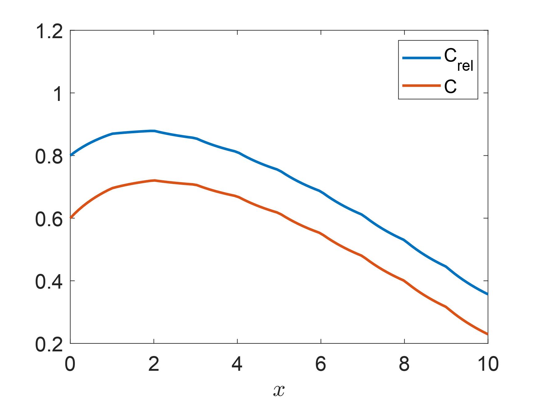
(b) $w=0.1$

Figure 2: Comparison of the original objective $C$ and the relaxed objective $C_{\text{rel}}$ for bang-bang policies. The policy parameters are related to the $x$-axis label as follows: $\ell=\left\lceil x\right\rceil,$ $p=p_{\max}-(\left\lceil x\right\rceil-x)(p_{\max}-p_{\min}).$ Chosen system parameters are as follows: $\lambda=2,$ $p_{\min}=1,$ $p_{\max}=2,$ $\beta=3.5,$ $\alpha=1.$

III Queueing Model

Consider a discrete time system, where the arrival rate for servers is insensitive to price and is equal to $\lambda(t)=\lambda$ for each time $t$. The customers respond to price set by the platform, and the arrival rate of customers in any time slot $t$ is $\mu(p(t))$ if the price chosen by the platform is $p(t)$ at time $t$. We assume the natural model, where $\mu(p)$ is a non-increasing continuous function of $p$. In addition, we assume that $\mu(p)$ is a concave function, and $p\mu(p)$ is a unimodal function of $p$, following prior work [11]. Recall that for notational convenience in Section II, we assumed that the customer arrival rate is $\mu=g(p)$, while in this section, we use simply $\mu(p)$.

Under this model, let $A(t)$ and $B(t)$ be the number of servers and customers that arrive in time slot $t$, following i.i.d. processes, with rate $\lambda$ and $\mu(p(t))$, respectively. In particular, $\lambda={\mathbb{E}}\{A(t)\}$ and $\mu(p(t))={\mathbb{E}}\{B(t)\}$. Let $M(t)$ be the set of customers that depart (number of customer-server pairs that are matched) at time $t$. Since there are two queues corresponding to servers and customers, making both queues stable (that allows the existence of steady state distribution) simultaneously is not possible without some exogenous constraint (unless we have a separate price lever for each queue, as is done in [10]). So to keep the server queue stable, we consider an upper limit ${\bar{S}}$ on the number of outstanding servers, while ensuring the stability of customer queue will be part of the considered problem. Thus, a server arriving when the server queue size is ${\bar{S}}$ is not admitted.

The number of servers $S(t)$, and customers $C(t)$, in the system at time $t$, evolve as follows.

$$S(t+1) =\min\{(S(t)+A(t)-|M(t)|)^{+},{\bar{S}}\},$$ (7)

$$C(t+1) =(C(t)+B(t)-|M(t)|)^{+},$$ (8)

where $|M(t)|$ is the number of customer-server pairs that are matched by the platform in time slot $t$, and $(x)^{+}=\max\{0,x\}$. The evolution of $S(t)$ and $C(t)$ is hence coupled via $M(t)$.

Remark 6.

Compared to Section II, where we considered a loss model, in this section, customers wait in the queue, and depart only when they are matched to any server. Moreover, we are considering a more general system than Section II, that evolves in discrete time, and the customer and server arrival processes are not restricted to follow a Poisson distribution.

Customer $i$ arriving at time $t$ sees or commits to price $p_{i}=p(t)$, and let the platform make profit of $p_{i}$ when customer $i$ is matched (departs) to some server at time $t^{\prime}\geq t$. Thus, the profit made by the platform at time $t$ is determined by the set of $M(t)$ customers that depart at time $t$, and the price they saw when they arrived $p_{i},i\in M(t)$. Thus, given the price $p(t)$ chosen by the platform, its profit (that is a function of price $p(t)$) is given by

$${\mathbf{V}}=\lim_{T\rightarrow\infty}\frac{1}{T}\sum_{t=1}^{T}V\left(\sum_{i\in M(t)}p_{i}\right),$$ (9)

where $V$ is a non-decreasing concave function.

Note that in defining the platform’s profit (9), we have not directly accounted for the payment to the servers, however, that is implicitly captured by assuming that the platform keeps a constant factor of the profit to itself and distributes the rest uniformly across all servers. Thus, maximizing profit, is equivalant to maximizing the payment to the servers. Servers not being incentivised per-customer matching is well justified following [1], which shows that servers payoffs are better modelled as long-term rewards.

The optimization problem that we consider is as follows.

$$\max_{p(t),M(t)}\quad{\mathbf{V}}\quad\text{s.t.}\ \underbrace{\lim_{T\rightarrow\infty}\frac{1}{T}\sum_{t=1}^{T}{\mathbb{E}}\{C(t)\}<\infty}_{\text{stability of customer queue}}.$$ (10)

The stability condition in (10) takes care of the fact that the delay seen by arriving customers is bounded.

Remark 7.

An alternate formulation to (10) is to maximize ${\mathbf{V}}$ subject to a constraint on the expected delay seen by the customers, or maximize a linear combination of ${\mathbf{V}}$ and expected delay seen by the customers. Both these alternatives are, however, more challenging to solve in the setting considered, where we are not considering any scaling limit regime, unlike [1] and similar papers. In what will follow, the algorithm we propose to solve (10), will have a parameter that will tradeoff the sub-optimality gap (Theorem 10) and the expected delay (Lemma 8) seen by the customers. Thus, given a constraint on the expected delay seen by the customers, we can tune the parameter and bound the sub-optimality gap.

Let the optimal price be $p^{\star}(t)$ and optimal matching decision be $M^{\star}(t)$ to maximize (10) under the stability constraint, and let the optimal profit be ${\mathbf{V}}_{\mathsf{OPT}}$. Next, we upper bound ${\mathbf{V}}_{\mathsf{OPT}}$. Towards that end, we define a critical quantity $p^{\star}$, as follows.

$$p^{\star}=\arg\max_{p,\lambda\geq\mu(p)}p\cdot\mu(p).$$ (11)

Note that since $\mu(p)$ is assumed to be a non-increasing continuous concave function of $p$, it follows that $p\mu(p)$ is a concave function. Using this fact, we get the following upper bound on ${\mathbf{V}}_{\mathsf{OPT}}$.

Lemma 5.

${\mathbf{V}}_{\mathsf{OPT}}\leq V(p^{\star}\mu(p^{\star})).$

Lemma 5 essentially says that the largest profit is possible if the price is set as constant $p^{\star}$, and the number of matched customer-server pairs $|M(t)|$ is a constant equal to the expected customer arrival rate $\mu(p^{\star})$ at price $p^{\star}$. The proof follows from a straightforward application of Jensen’s inequality, given that $V$ is a concave function.

Next, we propose an algorithm for setting the price $p(t)$, and choosing the number of matched customers $|M(t)|$ in each time slot $t$, and lower bound its profit.

Algorithm $\mathcal{A}$: Following the definitions of S(t) (7) and C(t) (8), let $N(t)=\min\{S(t),C(t)\}$. Solving (11), either we have $\lambda>\mu(p^{\star})$ or $\lambda=\mu(p^{\star})$.

If $\lambda>\mu(p^{\star})$, the algorithm chooses constant price $p(t)=p^{\star}$, $\forall\ t$, defined in (11), and the number of customer-server pairs matched in slot $t$ using FIFO schedule are

$$|M_{\mathcal{A}}(t)|=\begin{cases}0&\text{if}\ N(t)<\mu(p^{\star})-\delta,\\ \mu(p^{\star})-\delta&\text{if}\ \mu(p^{\star})-\delta\leq N(t)\leq U/2,\\ \mu(p^{\star})+\delta&\text{if}\ N(t)>U/2,\end{cases}$$ (12)

where $U<{\bar{S}}$ is some threshold, and $\delta>0$ that will be chosen later. Threshold $U$ will control both the profit made by the platform as well as the expected waiting time of any customer.

If $\lambda=\mu(p^{\star})$, then $p(t)=p^{\star}+\epsilon$ (to ensure that the customer arrival rate is lower than the server arrival rate), while choice of $|M_{\mathcal{A}}(t)|$ remains unchanged as in (12).

For the rest of this section, we consider the case when $\lambda>\mu(p^{\star})$. All results will go through even when $\lambda=\mu(p^{\star})$ with an additional $O(\epsilon)$ penalty.

Remark 8.

Note that we are not enforcing the integrality constraint on $|M_{\mathcal{A}}(t)|$, similar to prior works [29, 30] on dynamic decision problems with server-customer queues, where the consideration is that the number of servers/customers is large enough at an aggregate scale, and $|M_{\mathcal{A}}(t)|$ can be thought of as the fraction of customers served.

With algorithm $\mathcal{A}$, for both cases, $\lambda>\mu(p^{\star})$ or $\lambda=\mu(p^{\star})$, the arrival rate of servers is more than the arrival rate of customers with the algorithm, ensuring stability of the customer queue, satisfying the constraint in (10). Thus, we only need to derive a lower bound on the profit of algorithm $\mathcal{A}$, for which we need the following definition. Let $\sigma^{2}_{C}=\lim_{T\rightarrow\infty}\frac{1}{T}\text{var}\left(\sum_{t=1}^{T}B(t)\right)$ be the variance of process $B(t)$, number of arrivals of customers at time $t$.

Remark 9.

With the algorithm $\mathcal{A}$ that charges price $p(t)=p^{\star}$, the process $B(t)$ (the number of customer arrivals with mean $\mu(p^{\star})$) is an i.i.d. process. Therefore, $\sigma^{2}_{C}$ is well-defined.

The main result of this section is the following.

Theorem 10.

Choosing $\delta=\alpha\left(\frac{\log U}{U}\right),$ where $\alpha=\beta\sigma^{2}_{C}$ and $\beta\geq 2$, for algorithm $\mathcal{A}$,

$${\mathbf{V}}_{\mathcal{A}}\geq{\mathbf{V}}_{\mathsf{OPT}}-{\mathcal{O}}\left(\left(\frac{\log U}{U}\right)^{2}\right).$$

Thus, algorithm $\mathcal{A}$ is near-optimal and the sub-optimality gap is governed by the choice of threshold $U$.

Proof Sketch: Let $N$ be distributed as as per the steady state distribution of $N(t)$ with algorithm $\mathcal{A}$. By definition, algorithm $\mathcal{A}$ can achieve profit close to $V(p^{\star}\mu(p^{\star}))$ (where ${\mathbf{V}}_{\mathsf{OPT}}\leq V(p^{\star}\mu(p^{\star}))$) as long as $N>\mu(p^{\star})-\delta$. So the main result is to show that for $\mathcal{A}$, $P_{\text{outage}}={\mathbb{P}}(N<\mu(p^{\star})-\delta)={\mathcal{O}}\left(U^{-\beta}\right)$ for $\delta=\alpha\left(\frac{\log U}{U}\right),$ where $\alpha=\beta\sigma^{2}_{C}$ and $\beta\geq 2$, which we prove in Lemma 6. ∎

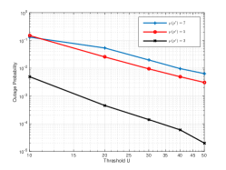
Figure 3: Outage probability with Poisson driver and customer arrivals with different values of $\mu(p^{\star})$ and $\Delta=.1$, respectively, as a function of $U$.

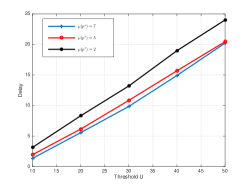
Figure 4: Expected delay experienced by a customer with Poisson driver and customer arrivals with different value of $\mu(p^{\star})$ and $\Delta=.1$, respectively, as a function of $U$.

Lemma 6.

For algorithm $\mathcal{A}$ (12) with price $p(t)=p^{\star},\ \forall\ t$,

$$P_{\text{outage}}={\mathbb{P}}(N<\mu(p^{\star})-\delta)={\mathcal{O}}\left(U^{-\beta}\right),$$

by choosing $\delta=\alpha\left(\frac{\log U}{U}\right),$ where $\alpha=\beta\sigma^{2}_{C}$ and $\beta\geq 2$.

Similar to the Lemma 6, we can get an upper bound on the $P(N\geq x)$ for $x\geq U$ as follows.

Lemma 7.

For algorithm $\mathcal{A}$ (12) with price $p(t)=p^{\star},\ \forall\ t$,

$${\mathbb{P}}(N\geq x)={\mathcal{O}}\left(U^{-\beta}\right)$$

by choosing $\delta=\alpha\left(\frac{\log U}{U}\right)$, where $\alpha=\beta\sigma^{2}_{C}$ and $\beta\geq 2$, and $x>U$.

Proof of Lemma 7 is identical to that of Lemma 6 and is omitted. An important consequence of Lemma 7 is a bound on the expected customer queue length, which using Little’s law gives a bound on the average delay seen by the customers.

Corollary 11.

${\mathbb{E}}\{N\}={\mathcal{O}}(U)$ by choosing $\beta\geq 3$.

Lemma 7 helps us in bounding the expected waiting time ${\mathbb{E}}\{W\}$ seen by any customer using Little’s Law. Recall that with algorithm $\mathcal{A}$, the customer arrival rate is constant $\mu(p^{\star})$, and the system is stable. Thus, the expected customer departure rate is also $\mu(p^{\star})$. Thus, using Little’s Law,

$${\mathbb{E}}\{W\}={\mathbb{E}}\{N\}/\mu(p^{\star})={\mathcal{O}}\left(\frac{U}{\mu(p^{\star})}\right).$$ (13)

Thus, we have proved the following lemma.

Lemma 8.

With algorithm $\mathcal{A}$, the expected waiting time ${\mathbb{E}}\{W\}$ seen by any customer is ${\mathbb{E}}\{W\}={\mathcal{O}}\left(\frac{U}{\mu(p^{\star})}\right).$

Discussion: The upshot of Theorem 10 is that near optimal profit can be obtained with static pricing, and advantage of dynamic pricing is arbitrarily small. Similar conclusions have been derived in earlier papers e.g., [1], with an objective function that is a sum of the platform profit and the expected delay seen by the servers, however, these results were shown in limiting regimes, such as scaling the number of customers and servers, and considering a fluid limit. Moreover, Lemma 8 shows that the static pricing policy that achieves near optimal profit has bounded expected delay for customers, as a function of the parameter $U$ that also controls the sub-optimality gap. Thus, threshold level $U$ provides a tradeoff between the sub-optimality gap from Theorem 10 and the expected delay seen by a customer (13), and can be appropriately chosen given QoS requirements.

In Figs. 3 and 4, we illustrate the tradeoff between the sub-optimality gap and the expected customer delay as a function of $U$, when both the customer and the server arrival distributions are Poisson. Recall that the sub-optimality gap is essentially controlled by the outage probability. Thus, we plot the outage probability and expected customer queue length (that controls the expected delay), as a function of $U$ for different values of $\mu(p^{\star})$ and $\Delta=\lambda-\mu(p^{\star})=0.1$. This way we avoid making specific choices of $V$ and $\mu$, while still capturing the quantities of interest. We observe that the simulated performance remains unchanged for higher values of $\Delta$, since the minimum of the two rates $\lambda$, $\mu(p^{\star})$, controls the performance. Hence to avoid cluttered plots, we only illustrate the $\Delta=0.1$ case. For simulations, we use $\beta=2$, $\sigma_{C}^{2}=2$ that completely defines algorithm $\mathcal{A}$’s choice of $\delta$. As promised by theory, the outage probability falls off as power-law with respect to $U$, while the expected delay is close to $U/2$.

IV Conclusions

In this paper, we have considered simple pricing strategies for two sided queue matching problems, that have typically been either analysed in large system limits, or for which optimal but non-closed form policies are known. We considered both the loss and the queueing systems, which are relevant for practical applications. For the loss system, we showed an important structural result that the optimal policy is of the bang bang type when the customer arrival rate is a linear function of the price. For the queueing model, we propose a simple static pricing strategy, and a bi-modal matching decision that is shown to be near-optimal, together with a bound on the expected delay seen by the customers.

V Appendices

V-A Proof of Lemma 1

Proof.

Under Assumption 1, we rewrite the first term of $C_{\text{rel}}$ as follows.

$$\sum_{i=0}^{\infty}\pi_{i}p_{i} =\frac{1}{\alpha}\sum_{i=0}^{\infty}\pi_{i}(\beta-\mu_{i})$$

$$=\frac{\beta-\pi_{0}\mu_{0}-\sum_{i=1}^{\infty}\pi_{i}\mu_{i}}{\alpha}$$

$$\stackrel{{\scriptstyle(a)}}{{=}}\frac{\beta-\pi_{0}\mu_{0}-\sum_{i=1}^{\infty}\pi_{i-1}\lambda}{\alpha}$$

$$=\frac{\beta-\pi_{0}\mu_{0}-\lambda}{\alpha}.$$

Step$(a)$ follows from the reversibility of the birth death Markov chain, which gives $\pi_{i-1}\lambda=\pi_{i}\mu_{i}$ for $i\geq 1.$ ∎

V-B Proof of Lemma 2

This section is devoted to the proof of Lemma 2, which shows that any feasible policy that does not have the above bang-bang structure can be improved upon by making a perturbation ‘towards this structure’. We start with the following lemma.

Lemma 9.

Assuming positive recurrence, for any $i\geq 1,$ $\pi(0)$ is a strictly decreasing function of $\rho_{i}$ and $\sum_{i=0}^{\infty}i\pi_{i}$ is a strictly increasing function of $\rho_{i}.$

The proof of Lemma 9 is trivial; we omit the proof.

Proof of Lemma 2.

If $\bar{\rho}<1$ and $\frac{\bar{\rho}}{1-\bar{\rho}}\leq C,$ then the optimal solution, in light of Lemma 9, is: $\rho_{i}=\bar{\rho}$ for all $i$ (i.e., $\ell^{*}=\infty$).

Thus, in the remainder of this proof, we assume that either (i) $\bar{\rho}\geq 1,$ or (ii) $\bar{\rho}<1$ and $\frac{\bar{\rho}}{1-\bar{\rho}}>C.$ In this case, in light of Lemma 9, moment constraint in (3) must hold with equality at the optimum.

Let

$$f(\rho) :=\frac{1}{\pi_{0}}=\sum_{j=0}^{\infty}h_{j},$$

$$m(\rho) :=\sum_{i=0}^{\infty}(i-C)h_{i}.$$

Denoting the optimal solution of (3) by $\rho^{*},$ note that $m(\rho^{*})=0.$

The statement of the lemma now follows from the following claim.

Claim 1: Consider $\rho=(\rho_{i},\ i\geq 1)$ such that

• $m(\rho)=0,$ and

• there exists $i\geq 1$ satisfying $\rho_{i}<\bar{\rho},$ $\rho_{i+1}>\underline{\rho}.$

Then $\rho$ is not optimal. Specifically, one can construct $\tilde{\rho}$, where $\tilde{\rho}_{j}=\rho_{j}$ for $j\neq i,i+1,$ and for $\epsilon,\delta>0,$ $\tilde{\rho}_{i}=\rho_{i}+\epsilon,$ $\tilde{\rho}_{i+1}=\rho_{i-1}-\delta,$ such that $m(\tilde{\rho})=0,$ $f(\tilde{\rho})>f(\rho).$

Proof of Claim 1: First, consider the difference $f(\tilde{\rho})-f(\rho).$

$$f(\tilde{\rho})-f(\rho) = \sum_{j}\tilde{h}_{j}-\sum_{j}h_{j}=h_{i-1}\left((\tilde{\rho}_{i}-\rho_{i})+\sum_{j\geq i+1}^{\infty}\left(\prod_{k=i}^{j}\tilde{\rho}_{k}-\prod_{k=i}^{j}\rho_{k}\right)\right)$$ (14)

$$= h_{i-1}\bigg{(}(\tilde{\rho_{i}}-\rho_{i})+(\tilde{\rho_{i}}\tilde{\rho}_{i+1}-\rho_{i}\rho_{i+1})+\sum_{j\geq i+2}^{\infty}(\tilde{\rho}_{i}\tilde{\rho}_{i+1}-\rho_{i}\rho_{i+1})\prod_{k=i+2}^{j}\rho_{k}\bigg{)}$$

$$= h_{i-1}\bigg{(}(\tilde{\rho}_{i}-\rho_{i})+(\tilde{\rho}_{i}\tilde{\rho}_{i+1}-\rho_{i}\rho_{i+1})\bigg{(}1+\sum_{j\geq i+2}^{\infty}\prod_{k=i+2}^{j}\rho_{k}\bigg{)}\bigg{)}.$$

Next, consider the difference $m(\tilde{\rho})-m(\rho).$

$$m(\tilde{\rho})-m(\rho) = \sum_{j}\tilde{h}_{j}(j-C)\ -\ \sum_{j}h_{j}(j-C)=\sum_{j}(\tilde{h}_{j}-h_{j})(j-C)$$

$$= h_{i-1}\bigg{(}(\tilde{\rho}_{i}-\rho_{i})(i-C)+(\tilde{\rho}_{i}\tilde{\rho}_{i+1}-\rho_{i}\rho_{i+1})\bigg{(}(i+1-C)+\sum_{j\geq i+2}(j-C)\prod_{k=i+2}^{j}\rho_{k}\bigg{)}\bigg{)}.$$

Setting the above difference to zero gives us the following condition that relates the perturbations $\epsilon$ and $\delta.$

$$\tilde{\rho}_{i}\tilde{\rho}_{i+1}-\rho_{i}\rho_{i+1}=\frac{-(\tilde{\rho}_{i}-\rho_{i})(i-C)}{(i+1-C)+\sum_{j\geq i+2}(j-C)\prod_{k=i+2}^{j}\rho_{k}}.$$

Substituting the above into (14), we have

$$f(\tilde{\rho})-f(\rho) = h_{i-1}\bigg{(}(\tilde{\rho_{i}}-\rho_{i})-\frac{(\tilde{\rho}_{i}-\rho_{i})(i-C)\big{(}1+\sum_{j\geq i+2}^{\infty}\prod_{k=i+2}^{j}\rho_{k}\big{)}}{(i+1-C)+\sum_{j\geq i+2}(j-C)\prod_{k=i+2}^{j}\rho_{k}}\bigg{)}$$

$$=\ \frac{h_{i-1}(\tilde{\rho_{i}}-\rho_{i})}{(i+1-C)+\sum_{j\geq i+2}(j-C)\prod_{k=i+2}^{j}\rho_{k}}\bigg{(}1+\sum_{j\geq i+2}(j-i)\prod_{k=i+2}^{j}\rho_{k}\bigg{)}.$$

It thus suffices to show that

$$(i+1-C)+\sum_{j\geq i+2}(j-C)\prod_{k=i+2}^{j}\rho_{k}>0.$$ (15)

This is trivial if $i+1\geq C.$ Suppose then that $i+1<C.$ In this case, note that

$$m(\rho)=\sum_{j=0}^{i}(j-C)h_{j}+\sum_{j=i+1}^{\infty}(j-C)h_{j}=0.$$

Since the first term above is negative, it follows that the second is positive, i.e.,

$$\sum_{j=i+1}^{\infty}(j-C)h_{j}=h_{i+1}\left((i+1-C)+\sum_{j\geq i+2}(j-C)\prod_{k=i+2}^{j}\rho_{k}\right)>0,$$

which implies (15). ∎

V-C Proofs of results in Section II-D1

Proof of Lemma 3.

The proof follows by considering only the revenue component of the objective, and via an application of Jensen’s inequality.

$$C_{\text{rel}}\leq\sum_{i=0}^{\infty}\pi_{i}g^{-1}(\mu_{i})\leq g^{-1}\left(\sum_{i=0}^{\infty}\pi_{i}\mu_{i}\right)\leq g^{-1}(\lambda).$$

In the last step above, we use $\lambda=\sum_{i=1}^{\infty}\pi_{i}\mu_{i}\leq\sum_{i=0}^{\infty}\pi_{i}\mu_{i}.$ ∎

Proof of Lemma 4.

Consider a tagged server arriving into the system in steady state. If the server is matched at price $p,$ its mean sojourn time is at least $\frac{1}{g(p)}.$ Optimizing with respect to $p$ yields the upper bound. Since we are ignoring congestion from other (waiting) servers, this bound is expected to be tight in light traffic. ∎

V-D Proof of Lemma 5

Proof.

Consider stationary Markov policies which apply a finite collection of prices $\{p_{k},\ k\in\mathcal{K}\},$ such that the long run fraction of time price $p_{k}$ is used by the platform is $\theta_{k}>0.$ Since the customer queue must be stable, we have

$$\lambda\geq\sum_{k\in\mathcal{K}}\theta_{k}\mu(p_{k}).$$

Let $N_{k,t}$ denote the number of times price $p_{k}$ has been used until time $t,$ and $B_{k,i}$ is the random number of customer arrivals that take place the $i$th time price $p_{k}$ is used. Clearly, $\{B_{k,i}\}_{i\geq 1}$ is an i.i.d. sequence with mean $\mu(p_{k}).$ Using this, we bound the objective as follows.

$$\frac{1}{T}\sum_{t=1}^{T}V(\sum_{i\in M(t)}p_{i}) \leq V\left(\frac{\sum_{t=1}^{T}\sum_{i\in M(t)}p_{i}}{T}\right)$$

$$=V\left(\frac{\sum_{t=1}^{T}p(t)B(t)-\sum_{j\in C(t+1)}p_{j}}{T}\right)$$

$$=V\left(\frac{\sum_{k\in\mathcal{K}}p_{k}\sum_{i=1}^{N_{k,t}}B_{k,i}-\sum_{j\in C(t+1)}p_{j}}{T}\right)$$

$$=V\left(\sum_{k\in\mathcal{K}}p_{k}\frac{\sum_{i=1}^{N_{k,t}}B_{k,i}}{N_{k,t}}\frac{N_{k,t}}{T}-\frac{\sum_{j\in C(t+1)}p_{j}}{T}\right)$$

Letting $T\rightarrow\infty,$ we get that almost surely,

$$\limsup_{T\rightarrow\infty}\frac{1}{T}\sum_{t=1}^{T}V(\sum_{i\in M(t)}p_{i}) \leq V\left(\sum_{k\in K}p_{k}\mu(p_{k})\theta_{k}\right)$$

$$\leq V\left(p^{\star}\mu(p^{\star})\right).$$

The last step above uses the concavity of the function $p\mu(p).$ ∎

V-E Proof of Theorem 10

Proof.

With algorithm $\mathcal{A}$ (12), since a constant price $p(t)=p^{\star}$ is charged to all the customers, we rewrite the profit (9) as

$${\mathbf{V}}_{\mathcal{A}}=\lim_{T\rightarrow\infty}\frac{1}{T}\sum_{t=1}^{T}V(p^{\star}|M_{\mathcal{A}}(t)|).$$ (16)

Note that this rewriting of the profit (9) is possible only for algorithms that charge a constant price across time, however, ${\mathbf{V}}_{\mathsf{OPT}}$ allows arbitrary pricing $p(t)$.

Next, we show that

$$\lim_{T\rightarrow\infty}\frac{1}{T}\sum_{t=1}^{T}V(p^{\star}|M_{\mathcal{A}}(t)|)\geq V(p^{\star}\mu(p^{\star}))-O\left(\left(\frac{\log U}{U}\right)^{2}\right).$$

Let $V^{+}$ and $V^{-}$ be the profit made by the algorithm $\mathcal{A}$ when $N\geq U/2$ by using $|M_{\mathcal{A}}(t)|=\mu(p^{\star})+\delta$, and when $N<U/2$ (assuming $N(t)>\mu(p^{\star})-\delta$), with $|M_{\mathcal{A}}(t)|=\mu(p^{\star})-\delta$, respectively. The Taylor series expansion of the profit ($V^{+}$ and $V^{-}$) about $p^{\star}\mu(p^{\star})$ can be written as

$$\begin{split}V^{+}=V(p^{\star}(\mu(p^{\star})+\delta))&=V\left(p^{\star}\mu(p^{\star})\right)+V^{(1)}\left(p^{\star}\mu(p^{\star})\right)\delta^{\prime}+V^{(2)}\left(p^{\star}\mu(p^{\star})\right)\delta^{\prime 2}+o(\delta^{\prime 2}),\end{split}$$ (17)

$$\begin{split}V^{-}=V(p^{\star}(\mu(p^{\star})-\delta))&=V\left(p^{\star}\mu(p^{\star})\right)-V^{(1)}\left(p^{\star}\mu(p^{\star})\right)\delta^{\prime}+V^{(2)}\left(p^{\star}\mu(p^{\star})\right)\delta^{\prime 2}+o(\delta^{\prime 2}).\end{split}$$ (18)

where $V^{(i)}$ is the $i^{th}$ derivative of $V$ and $\delta^{\prime}=p^{\star}\delta$.

Define $\rho^{+}$ as the fraction of time that $N>\frac{U}{2}$, and $\rho^{-}$ as the fraction of time that $N\leq\frac{U}{2}$. Then the profit (16) can be written as

$${\mathbf{V}}_{\mathcal{A}} \stackrel{{\scriptstyle(a)}}{{=}}\rho^{+}V^{+}+\left(\rho^{-}-P_{\text{outage}}\right)V^{-},$$

$$\begin{split}&\stackrel{{\scriptstyle(b)}}{{=}}V(p^{\star}\mu(p^{\star}))+V^{(1)}(p^{\star}\mu(p^{\star}))(\rho^{+}\delta^{\prime}-\rho^{-}\delta^{\prime})+\Theta\left(\frac{(\log U)^{2}}{U^{2}}\right),\end{split}$$ (19)

where (a) follows from the fact that at most $|M_{\mathcal{A}}(t)|=\mu(p^{\star})-\delta$ when $N<U/2$ and $V^{-}$ is overestimated, (b) follows from (17) and (18) and Lemma 6, i.e., $P_{\text{outage}}=\Theta\left(U^{-\beta}\right)$, with $\delta=\Theta\left(\frac{\log U}{U}\right)$, $\rho^{+}+\rho^{-}=1$, and $V^{(2)}(\mu(p^{\star}))$ is constant.

By applying the conservation of customer arrivals, i.e., the departed customers is equal to the arrived customers, we have $\rho^{+}\left(\mu(p^{\star})+\delta\right)+(\rho^{-}-P_{\text{outage}})\left(\mu(p^{\star})-\delta\right)=\mu(p^{\star})$, following (12).

Rearranging this, and substituting the expression for $P_{\text{outage}}$ from Lemma 6, we get

$$\rho^{+}\delta-\rho^{-}\delta=\Theta\left(U^{-\beta}\right).$$ (20)

Using (20), from (19),

$${\mathbf{V}}_{\mathcal{A}} \stackrel{{\scriptstyle(a)}}{{\geq}}V(p^{\star}\mu(p^{\star}))+\Theta\left(U^{-\beta}\right)+\Theta\left(\frac{(\log U)^{2}}{U^{2}}\right).$$

From Lemma 5, ${\mathbf{V}}_{\mathsf{OPT}}\leq V(p^{\star}\mu(p^{\star}))$. Hence, we get that

$${\mathbf{V}}_{\mathsf{OPT}}-V_{\mathcal{A}}\leq\Theta\left(\frac{(\log U)^{2}}{U^{2}}\right),$$

since $\beta\geq 2$. ∎

Next, provide the remaining proof of Lemma 6.

Proof of Lemma 6.

Let the event $N<\mu(p^{\star})-\delta$ be called as the outage event. Since we are letting $U$ large, the outage event is similar to $N=0$. Hence, we will try to bound the outage probability ${\mathbb{P}}(N=0)=\lim_{T\rightarrow\infty}\frac{1}{T}\sum_{t=1}^{T}{\mathbb{P}}(N(t)=0)$.

We will break the time into intervals $\mathcal{I}$, where each interval has $\frac{U}{2L}>1$ time slots, and $L$ is some constant to be chosen later. Without loss of generality, we let $\frac{U}{2L}$ to be an integer. We call slot $t\in\mathcal{I}_{i}$ if slot $t$ falls in the interval $\mathcal{I}_{i}=[i\frac{U}{2L},\ \ (i+1)\frac{U}{2L}]$. Let the system be in operation since time $-\infty$.

Then event $E_{i}$ is defined as $N(0)=0$ and $\mathcal{I}_{-i}$ be the last interval during which $N(t)\geq U/2$, i.e., $t\in\mathcal{I}_{-i}$.

The basic idea in defining $E_{i}$, is that throughout time consisting of $i$ intervals, starting from interval $\mathcal{I}_{-i}$ till interval $\mathcal{I}_{0}$, the algorithm (12) will be using $|M_{\mathcal{A}}(t)|=\mu(p^{\star})-\delta$ since $N(t)\geq U/2$ throughout, while the arrival process $N(t)$ has increments with mean at least $\mu(p^{\star})$. Thus, there is a positive bias to the process $N(t)$, during interval $\mathcal{I}_{-i}$ till interval $\mathcal{I}_{0}$, and hence the probability $P(E_{i})$ is expected to be exponentially small with respect to $U$.

Under these definitions,

$${\mathbb{P}}(N=0)=\sum_{i=0}^{\infty}P(E_{i}).$$

We define two events that only depend on server arrivals $A(t)$ and customer arrivals $B(t)$ in time slot $t$, respectively. Let

$$F_{i1}:\sum_{t=-i\frac{U}{2L}}^{0}\left(|M_{\mathcal{A}}(t)|-B(t)\right)>U/2,$$

and

$$F_{i2}:\sum_{t=-i\frac{U}{2L}}^{0}\left(|M_{\mathcal{A}}(t)|-A(t)\right)>U/2.$$

We claim that event $E_{i}$ implies that at least one of $F_{i1}$ or $F_{i2}$, since the arrivals for either $A(t)$ or $B(t)$ are insufficient compared to $|M_{\mathcal{A}}(t)|$ for event $F_{i1}$ or $F_{i2}$ to happen.

To prove the claim consider the following two cases. The condition we know is that at time $t$, $N(t)=\min\{S(t),C(t)\}=U/2$. Case I : $S(t)=U/2$ and $C(t)\geq U/2$. Therefore, if both $F_{i1}$ and $F_{i2}$ are false, then $N(0)>0$, and hence $E_{i}$ is also false. Identical argument holds when Case II : $S(t)\geq U/2$ and $C(t)=U/2$.

Thus, we have that $E_{i}$ implies $F_{i1}\cup F_{i2}$, and therefore $P(E_{i})\leq P(F_{i1})+P(F_{i2})$.

Moreover, since $B(t)$ (with arrival rate $\lambda>\mu(p^{\star}))$ stochastically dominates $A(t)$ (with arrival rate $\mu(p^{\star})$), we have $P(F_{i1})\leq P(F_{i2})$. Hence, we have

$$P(E_{i})\leq 2P(F_{i2}).$$

B(t)

Next, we upper bound $P(F_{i2})$ using Chernoff’s bound as follows, where the proof is similar to [31], and is provided for completeness..

We begin by noting that $P(F_{i1})=P\left(\sum_{t=-i\frac{U}{2L}}^{0}\left(|M_{\mathcal{A}}(t)|-B(t)\right)>U/2\right)$ and

$P\left(\sum_{t=-i\frac{U}{2L}}^{0}\left(|M_{\mathcal{A}}(t)|-B(t)\right)>U/2\right)$

$$\stackrel{{\scriptstyle(a)}}{{\leq}} {\mathbb{E}}\left\{\exp\left(\theta_{i}\sum_{t=-i\frac{U}{2L}}^{0}\left(|M_{\mathcal{A}}(t)|-B(t)\right)\right)\right\}\exp\left(-\theta_{i}U/2\right)$$ (21)

$$\stackrel{{\scriptstyle(b)}}{{\leq}} {\mathbb{E}}\left\{\exp\left(-\theta_{i}\sum_{t=-i\frac{U}{2L}}^{0}B(t)\right)\right\}\exp\left(\theta_{i}\frac{U}{2L}\left(\mu(p^{\star})-\delta\right)\right)\exp\left(-\theta_{i}U/2\right),$$ (22)

$$\stackrel{{\scriptstyle(b)}}{{=}} \exp\left(-\frac{U}{2}\left(\theta_{i}\left(1-\frac{i+1}{L}(\mu(p^{\star})-\delta)\right)-\frac{i+1}{L}\mathcal{M}_{C}(-\theta_{i})+\epsilon_{i}(U,\theta_{i})\right)\right),$$ (23)

where $(a)$ follows from Chernoff’s bound for $\theta_{i}\geq 0$, $(b)$ follows since $|M_{\mathcal{A}}(t)|\leq\mu(p^{\star})-\delta$ for all slots $t$ from $-i\frac{U}{2L}$ till $0$, where for $(c)$ we define $\mathcal{M}_{C}(s)=\lim_{T\rightarrow\infty}\frac{1}{T}{\mathbb{E}}\left\{\exp\left(s\sum_{t=1}^{T}B(t)\right)\right\}$ as the semi-invariant log-moment generating function of $B(t)$ the number of customer arrivals in slot $t$, and $\epsilon_{i}(U,\theta_{i})\rightarrow 0$ as $U\rightarrow\infty$. Note that $\epsilon_{i}(U,\theta_{i})$ appears since the limit of the summation in $(a)$ is from $t=-i\frac{U}{2L}$ to $0$, and not from $t=0$ to $\infty$ and no limits are taken.

From (23), let $f_{i}(\theta)=\left(\theta\left(1-\frac{i+1}{L}(\mu(p^{\star})-\delta)\right)-\frac{i+1}{L}\mathcal{M}_{C}(-\theta)\right),$ and

$$\theta_{i}^{*}=\arg\max_{\theta}f_{i}(\theta).$$

Note that ${\mathbb{E}}\{B(t)\}=\mu(p^{\star})>\mu(p^{\star})-\delta$. Hence the function $\theta(\mu(p^{\star})-\delta)+\mathcal{M}_{C}(-\theta)$ has a negative slope at $\theta=0$. Hence, there exists a $\theta^{\prime}$ such that $\theta^{\prime}(\mu(p^{\star})-\delta)+\mathcal{M}_{C}(\theta^{\prime})<0$. Moreover, we get that for such a $\theta^{\prime}$, there exists ${\mathsf{i}}$ such that for $i\geq{\mathsf{i}}$ and $\gamma>0$, such that

$$f_{i}(\theta^{\prime})\geq f_{\mathsf{OPT}}+{\mathsf{i}}\gamma,$$ (24)

where

$$f_{\mathsf{OPT}}=\inf_{i\geq 0}\sup_{\theta\geq 0}f_{i}(\theta).$$

Recall that

$${\mathbb{P}}(N=0)=\sum_{i=0}^{\infty}P(E_{i})\leq 2\sum_{i=0}^{\infty}P(F_{i2}).$$ (25)

Writing a partial sum $P(F_{i2})$ for $i\geq{\mathsf{i}}$ from (23),

$$\sum_{i\geq{\mathsf{i}}}P(F_{i2}) \leq\sum_{i\geq{\mathsf{i}}}\exp\left(-\frac{U}{2}\left(\theta_{i}\left(1-\frac{i+1}{L}(\mu(p^{\star})-\delta)\right)-\frac{i+1}{L}\mathcal{M}_{C}(\theta_{i})+\epsilon_{i}(U,\theta_{i})\right)\right),$$

$$\leq\sum_{i\geq{\mathsf{i}}}\exp\left(-\frac{U}{2}\left(f_{i}(\theta^{\prime})+\epsilon_{i}(U,\theta^{\prime})\right)\right),$$ (26)

$$\stackrel{{\scriptstyle(a)}}{{\leq}}\sum_{i\geq{\mathsf{i}}}\exp\left(-\frac{U}{2}\left(f_{\mathsf{OPT}}+{\mathsf{i}}\gamma+\inf_{i\geq{\mathsf{i}}}\epsilon_{i}(U,\theta^{\prime})\right)\right),$$ (27)

$$=\exp\left(-f_{\mathsf{OPT}}\frac{U}{2L}\right)\frac{\exp\left(-\frac{U}{2}\left(({\mathsf{i}}+1)\gamma+\inf_{i>{\mathsf{i}}}\epsilon_{i}(U,\theta^{\prime})\right)\right)}{1-\exp\left(-\gamma\frac{U}{2}\right)},$$ (28)

where $(a)$ follows from (24). Thus, $\sup_{U\rightarrow\infty}\frac{2}{U}\log(\sum_{i\geq{\mathsf{i}}}P(F_{i1}))=0$.

The sum of $P(F_{i2})$ for the first ${\mathsf{i}}-1$ terms is at most

$$\sum_{i<{\mathsf{i}}}P(F_{i2}) \leq\sum_{i<{\mathsf{i}}}\exp\left(-\frac{U}{2}\left(\theta_{i}\left(1-\frac{i+1}{L}(\mu(p^{\star})-\delta)\right)-\frac{i+1}{L}\mathcal{M}_{C}(\theta_{i})+\epsilon_{i}(U,\theta_{i})\right)\right),$$

$$\leq\sum_{i\leq{\mathsf{i}}}\exp\left(-f_{\mathsf{OPT}}\frac{U}{2}\right)\left(({\mathsf{i}}+1)\min_{0\leq i<{\mathsf{i}}}\exp(\epsilon_{i}(U,\theta_{i}^{*})\right).$$ (29)

Combining, (28) and (29),

$$\sup_{U\rightarrow\infty}\frac{2}{U}\log(\sum_{i=0}^{\infty}P(F_{i2}))=-f_{\mathsf{OPT}}.$$

Thus, from (25)

$$\sup_{U\rightarrow\infty}\frac{2}{U}\log{\mathbb{P}}(N=0)\leq-f_{\mathsf{OPT}}.$$ (30)

This is true for all values of $L$, thus we let $L\rightarrow\infty$, and tighten the bound (30) as follows by using the definition of $f_{\mathsf{OPT}}$.

$$\sup_{U\rightarrow\infty}\frac{2}{U}\log{\mathbb{P}}(N=0)\leq-f_{\mathsf{OPT}}= -\inf_{i\geq 0}\sup_{\theta\geq 0}f_{i}(\theta),$$ (31)

$$= \inf_{i\geq 0}\sup_{\theta\geq 0}\left(\theta\left(1-\frac{i}{L}(\mu(p^{\star})-\delta)\right)-\frac{i}{L}\mathcal{M}_{C}(-\theta)\right),$$ (32)

$$= \inf_{T\geq 0}\sup_{\theta\geq 0}\left(\theta\left(1-T(\mu(p^{\star})-\delta)\right)-T\mathcal{M}_{C}(-\theta)\right),$$ (33)

$$= \inf_{T\geq 0}\sup_{\theta\geq 0}T\left(-\theta\left(-\frac{1}{T}+(\mu(p^{\star})-\delta)\right)-\mathcal{M}_{C}(-\theta)\right).$$ (34)

This infimum and supremum is achieved at $T=\tau^{*}$ and $\theta=T$, where $\tau^{*}$ is such that $\mathcal{M}_{C}(-\tau^{*})=\tau^{*}(\mu(p^{\star})-\delta)$.

Hence, we get that

$$\sup_{U\rightarrow\infty}\frac{2}{U}\log{\mathbb{P}}(N=0)\leq-\tau^{*}.$$

Rewriting $\tau^{*}$ as the root of $g(\tau)=\mathcal{M}_{C}(-\tau^{*})-\tau^{*}(\mu(p^{\star})-\delta)$, Lemma 10 implies that $\frac{d\tau^{*}}{d\delta}=-\frac{2}{\sigma^{2}_{C}}+o(\delta)$. Thus, we get $\tau^{*}=\frac{2\delta}{\sigma^{2}_{C}}+o(\delta)$.

Therefore, choosing $\delta=\alpha\frac{\log U}{U}$ and $\alpha=\beta\sigma^{2}_{C}$ for $\beta\geq 2$, we get

$${\mathbb{P}}(N=0)=O(U^{-\beta}).$$

∎

Lemma 10.

$$\frac{d\tau^{*}}{d\delta}\Bigr{|}_{\delta=0}=-\frac{2}{\sigma^{2}_{C}},$$

where $\sigma^{2}_{C}=\lim_{T\rightarrow\infty}\frac{1}{T}\text{var}\left(\sum_{t=1}^{T}B(t)\right)$, the variance of process $B(t)$, the number of arrivals of customers.

Recall that since the price $p(t)$ is a constant, process $B(t)$ is an i.i.d. process and $\sigma^{2}_{C}$ is well defined.

References

- [1] S. Banerjee, R. Johari, and C. Riquelme, “Pricing in ride-sharing platforms: A queueing-theoretic approach,” in Proceedings of the Sixteenth ACM Conference on Economics and Computation, 2015, pp. 639–639.
- [2] I. C. Paschalidis and J. N. Tsitsiklis, “Congestion-dependent pricing of network services,” IEEE/ACM transactions on networking, vol. 8, no. 2, pp. 171–184, 2000.
- [3] D. W. Low, “Optimal pricing for an unbounded queue,” IBM Journal of research and Development, vol. 18, no. 4, pp. 290–302, 1974.
- [4] S. Stidham Jr and R. R. Weber, “Monotonic and insensitive optimal policies for control of queues with undiscounted costs,” Operations research, vol. 37, no. 4, pp. 611–625, 1989.
- [5] J. M. George and J. M. Harrison, “Dynamic control of a queue with adjustable service rate,” Operations research, vol. 49, no. 5, pp. 720–731, 2001.
- [6] B. Ata and S. Shneorson, “Dynamic control of an M/M/1 service system with adjustable arrival and service rates,” Management Science, vol. 52, no. 11, pp. 1778–1791, 2006.
- [7] K. M. Adusumilli and J. J. Hasenbein, “Dynamic admission and service rate control of a queue,” Queueing Systems, vol. 66, no. 2, pp. 131–154, 2010.
- [8] J. Kim and R. S. Randhawa, “The value of dynamic pricing in large queueing systems,” Operations Research, vol. 66, no. 2, pp. 409–425, 2018.
- [9] L. M. Nguyen and A. L. Stolyar, “A queueing system with on-demand servers: local stability of fluid limits,” Queueing Systems, vol. 89, no. 3, pp. 243–268, 2018.
- [10] S. Mahavir Varma, P. Bumpensanti, S. Theja Maguluri, and H. Wang, “Dynamic pricing and matching for two-sided queues,” ACM SIGMETRICS Performance Evaluation Review, vol. 48, no. 1, pp. 105–106, 2020.
- [11] M. Sood, S. Moharir, and A. A. Kulkarni, “Pricing in two-sided markets in the presence of free upgrades,” in COMSNETS, 2018.
- [12] Y. Kanoria and P. Qian, “Near optimal control of a ride-hailing platform via mirror backpressure,” arXiv preprint arXiv:1903.02764, 2019.
- [13] C. Yan, H. Zhu, N. Korolko, and D. Woodard, “Dynamic pricing and matching in ride-hailing platforms,” Naval Research Logistics (NRL), vol. 67, no. 8, pp. 705–724, 2020.
- [14] O. Besbes, F. Castro, and I. Lobel, “Surge pricing and its spatial supply response,” Management Science, 2020.
- [15] B. Hu, M. Hu, and H. Zhu, “Surge pricing and two-sided temporal responses in ride hailing,” Available at SSRN 3278023, 2020.
- [16] R. Caldentey, E. H. Kaplan, and G. Weiss, “FCFS infinite bipartite matching of servers and customers,” Advances in Applied Probability, vol. 41, no. 3, pp. 695–730, 2009.
- [17] I. Adan and G. Weiss, “Exact fcfs matching rates for two infinite multitype sequences,” Operations research, vol. 60, no. 2, pp. 475–489, 2012.
- [18] I. Gurvich and A. Ward, “On the dynamic control of matching queues,” Stochastic Systems, vol. 4, no. 2, pp. 479–523, 2015.
- [19] M. Hu and Y. Zhou, “Dynamic type matching,” Rotman School of Management Working Paper, no. 2592622, 2020.
- [20] Y. Chen and M. Hu, “Pricing and matching with forward-looking buyers and sellers,” Manufacturing & Service Operations Management, vol. 22, no. 4, pp. 717–734, 2020.
- [21] M. S. Lobo and S. Boyd, “Pricing and learning with uncertain demand,” in INFORMS Revenue Management Conference, 2003.
- [22] A. Roy, V. Borkar, A. Karandikar, and P. Chaporkar, “Online reinforcement learning of optimal threshold policies for markov decision processes,” arXiv preprint arXiv:1912.10325, 2019.
- [23] M. L. Puterman, Markov decision processes: Discrete stochastic dynamic programming. John Wiley & Sons, 2014.
- [24] R. F. Serfozo, “Monotone optimal policies for markov decision processes,” in Stochastic Systems: Modeling, Identification and Optimization, II, 1976, pp. 202–215.
- [25] R. Vaze and J. Nair, “Non-asymptotic near optimal algorithms for two sided matchings,” 2022. [Online]. Available: www.ee.iitb.ac.in/\~jayakrishnan.nair/papers/TwoSidedQueues.pdf
- [26] K. Chaudhary, V. Kavitha, and J. Nair, “Dynamic scheduling in a partially fluid, partially lossy queueing system,” 2019. [Online]. Available: https://arxiv.org/abs/1904.06480
- [27] A. Wierman, L. L. Andrew, and A. Tang, “Power-aware speed scaling in processor sharing systems: Optimality and robustness,” Performance Evaluation, vol. 69, no. 12, pp. 601–622, 2012.
- [28] R. Vaze and J. Nair, “Multiple server srpt with speed scaling is competitive,” IEEE/ACM Transactions on Networking, vol. 28, no. 4, pp. 1739–1751, 2020.
- [29] M. Lin, A. Wierman, L. L. Andrew, and E. Thereska, “Dynamic right-sizing for power-proportional data centers,” IEEE/ACM Transactions on Networking, vol. 21, no. 5, pp. 1378–1391, 2012.
- [30] B. Berg, R. Vesilo, and M. Harchol-Balter, “heSRPT: Optimal parallel scheduling of jobs with known sizes,” arXiv preprint arXiv:1903.09346, 2019.
- [31] R. Srivastava and C. E. Koksal, “Basic performance limits and tradeoffs in energy-harvesting sensor nodes with finite data and energy storage,” IEEE/ACM Transactions on Networking, vol. 21, no. 4, pp. 1049–1062, 2012.