DCT Approximations Based on Chen’s Factorization

In this paper, two 8-point multiplication-free DCT approximations based on the Chen’s factorization are proposed and their fast algorithms are also derived. Both transformations are assessed in terms of computational cost, error energy, and coding gain. Experiments with a JPEG-like image compression scheme are performed and results are compared with competing methods. The proposed low-complexity transforms are scaled according to Jridi-Alfalou-Meher algorithm to effect 16- and 32-point approximations. The new sets of transformations are embedded into an HEVC reference software to provide a fully HEVC-compliant video coding scheme. We show that approximate transforms can outperform traditional transforms and state-of-the-art methods at a very low complexity cost.

Keywords
Approximate DCT, Chen’s factorization, Fast algorithms, Image and video compression, Low-complexity transforms

1 Introduction

Discrete transforms are very useful tools in digital signal processing and compressing technologies [10, 23]. In this context, the discrete cosine transform (DCT) plays a key role [2] since it is a practical approximation for the Karhunen-Loève transform (KLT) [15]. The KLT has the property of being optimal in terms of energy compaction when the intended signals are modeled after a highly correlated first-order Markov process [10]. This is a widely accepted supposition for natural images [17].

Particularly, the DCT type II (DCT-II) of order 8 is a widely employed method [10], being adopted in several industry standards of image and video compression, such as JPEG [17], MPEG-1 [40], MPEG-2 [25], H.261 [26], H.263 [27], H.264 [39], and the state-of-the-art HEVC [38]. Aiming at the efficient computation of the DCT, many fast algorithms have been reported in literature [12, 33, 43, 53]. Nevertheless, these methods usually need expensive arithmetic operations, as multiplications, and an arithmetic on floating point, demanding major hardware requirements [32].

An alternative to the exact DCT computation is the use of DCT approximations that employ integer arithmetic only and do not require multiplications [10, 23]. In this context, several approximations for the DCT-II were proposed in literature. Often the elements of approximate transform matrices are defined over the set $\mathcal{P}=\{0,\pm\frac{1}{2},\pm 1,\pm 2\}$ [20, 14]. Relevant methods include the signed DCT (SDCT) [20] and the Bouguezel-Ahmad-Swamy (BAS) series of approximations [7, 8, 9, 3].

Transform matrices with elements in $\mathcal{P}$ have null multiplicative complexity [5]. Thus their associate hardware implementations require only additions and bit-shifting operations [3]. This fact renders such multiplierless approximations suitable for hardware-software implementations on devices/sensors operating at low computational power and severe energy consumption constraints [11, 39, 40].

In this work, we aim at the following goals:

• the proposition of new multiplication-free approximations for the 8-point DCT-II, based on Chen’s algorithm [12];

• the derivation of fast algorithms for the introduced transforms;

• a comprehensive assessment of the new approximations in terms of coding and image compression performance compared to popular alternatives;

• the extension of the proposed 8-point transforms to 16- and 32-point DCT approximations by means of the scalable recursive method proposed in [29]; and

• the embedment of the obtained approximations into an HEVC-compliant reference software [28].

This paper unfolds as follows. Section 2 presents Chen’s factorization for the 8-point DCT-II. In Section 3, we present two novel 8-point multiplierless transforms and their fast algorithms. The proposed approximations are assessed and mathematically compared with competing methods in Section 4. Section 5 provides comprehensive image compression analysis based on a JPEG-like compression scheme. Several images are compressed and assessed for quality according to the approximate transforms. Section 6 extends the 8-point transforms to 16- and 32-point DCT approximations and considers a real-world video encoding scheme based on these particular DCT approximations. Final conclusions and remarks are drawn in Section 7.

2 Chen’s factorization for the DCT

Chen et al. [12] proposed a fast algorithm for the DCT-II based on a factorization for the DCT type IV (DCT-IV). These two versions of the DCT differ in the sample points of the cosine function used in their transformation kernel [48, 10]. The $(m,n)$-th element of the $N$-point DCT-II and DCT-IV transform matrices, respectively denoted as $\mathbf{C}_{N}^{\mbox{\scriptsize II}}$ and $\mathbf{C}_{N}^{\mbox{\scriptsize IV}}$, are given by:

$$\left[\mathbf{C}_{N}^{\mbox{\scriptsize II}}\right]_{m,n}= \left[\sqrt{\frac{2}{N}}\,\,c_{m}\cos\!\left(\frac{m(2n+1)\pi}{2N}\right)\right]_{m,n},$$

$$\left[\mathbf{C}_{N}^{\mbox{\scriptsize IV}}\right]_{m,n}= \left[\sqrt{\frac{2}{N}}\,\cos\!\left(\frac{(2m+1)(2n+1)\pi}{4N}\right)\right]_{m,n},$$

where $m,n=0,1,\ldots,N-1$ and

$$c_{m}=\left\{\begin{array}[]{cl}1/\sqrt{2},&\text{if $m=0$},\\ 1,&\text{if $m\neq 0$}.\\ \end{array}\right.$$

In the following, let $\mathbf{0}_{N}$ the zero matrix of order $N$, $\mathbf{I}_{N}$ the $N\times N$ identity and $\bar{\mathbf{I}}_{N}$ the counter-identity matrix, which is given by:

$$\bar{\mathbf{I}}_{N}=\left[\begin{smallmatrix}\ \ &\ \ &\ \ &\ \ \\ 0&\@cdots&0&1\\[1.42271pt] 0&\@cdots&1&0\\[1.42271pt] \@vdots&\udots&\@vdots&\@vdots\\[1.42271pt] 1&\@cdots&0&0\\[1.42271pt] \end{smallmatrix}\right].$$

In [47], Wang demonstrated that the 8-point DCT-II matrix possesses the following factorization:

$$\mathbf{C}_{8}^{\mbox{\scriptsize II}}=\frac{1}{2}\,\mathbf{P}_{8}\left[\begin{array}[]{cc}\mathbf{C}_{4}^{\mbox{\scriptsize II}}&\mathbf{0}_{4}\\ \mathbf{0}_{4}&\bar{\mathbf{I}}_{4}\,\mathbf{C}_{4}^{\mbox{\scriptsize IV}}\,\bar{\mathbf{I}}_{4}\\ \end{array}\right]\mathbf{B}_{8},$$ (1)

where $\mathbf{P}_{8}$ and $\mathbf{B}_{8}$ are permutation and pre-addition matrices given by, respectively:

$$\mathbf{P}_{8}=\left[\begin{smallmatrix}\ \ &\ \ &\ \ &\ \ &\ \ &\ \ &\ \ &\ \ \\[1.42271pt] 1&0&0&0&0&0&0&0\\[1.42271pt] 0&0&0&0&0&0&0&1\\[1.42271pt] 0&1&0&0&0&0&0&0\\[1.42271pt] 0&0&0&0&0&0&1&0\\[1.42271pt] 0&0&1&0&0&0&0&0\\[1.42271pt] 0&0&0&0&0&1&0&0\\[1.42271pt] 0&0&0&1&0&0&0&0\\[1.42271pt] 0&0&0&0&1&0&0&0\\[1.42271pt] \end{smallmatrix}\right],\ \mathbf{B}_{8}=\left[\begin{array}[]{rr}\mathbf{I}_{4}&\bar{\mathbf{I}}_{4}\\ \bar{\mathbf{I}}_{4}&-\mathbf{I}_{4}\\ \end{array}\right].$$

Additionally, Chen et al. suggested in [12] that the matrix $\mathbf{C}_{4}^{\mbox{\scriptsize IV}}$ admits the following factorization:

$$\mathbf{C}_{4}^{\mbox{\scriptsize IV}}=\mathbf{Q}\,\mathbf{A}_{1}\,\mathbf{A}_{2}\,\mathbf{A}_{3},$$ (2)

where

$$\mathbf{Q}=\left[\begin{smallmatrix}\ \ &\ \ &\ \ &\ \ \\ 1&0&0&0\\[1.42271pt] 0&0&1&0\\[1.42271pt] 0&1&0&0\\[1.42271pt] 0&0&0&1\\[1.42271pt] \end{smallmatrix}\right],\;\mathbf{A}_{1}=\left[\begin{smallmatrix}\ \ &\ \ &\ \ &\ \ \\ \beta_{0}&\phantom{-}0&\phantom{-}0&\phantom{-}\beta_{3}\\[1.42271pt] 0&\phantom{-}\beta_{2}&\phantom{-}\beta_{1}&\phantom{-}0\\[1.42271pt] 0&\phantom{-}\beta_{1}&-\beta_{2}&\phantom{-}0\\[1.42271pt] \beta_{3}&\phantom{-}0&\phantom{-}0&-\beta_{0}\\[1.42271pt] \end{smallmatrix}\right],\;\mathbf{A}_{2}=\left[\begin{smallmatrix}\ \ &\ \ &\ \ &\ \ \\ 1&\phantom{-}1&\phantom{-}0&\phantom{-}0\\[1.42271pt] 1&-1&\phantom{-}0&\phantom{-}0\\[1.42271pt] 0&\phantom{-}0&-1&\phantom{-}1\\[1.42271pt] 0&\phantom{-}0&\phantom{-}1&\phantom{-}1\\[1.42271pt] \end{smallmatrix}\right],\;\mathbf{A}_{3}=\left[\begin{smallmatrix}\ \ &\ \ &\ \ &\ \ \\ 0&\phantom{-}0&\phantom{-}0&\phantom{-}1\\[1.42271pt] 0&\phantom{-}\alpha&\phantom{-}\alpha&\phantom{-}0\\[1.42271pt] 0&-\alpha&\phantom{-}\alpha&\phantom{-}0\\[1.42271pt] 1&\phantom{-}0&\phantom{-}0&\phantom{-}0\\[1.42271pt] \end{smallmatrix}\right],$$

with $\alpha=\cos\!\left(\frac{\pi}{4}\right)$ and $\beta_{n}=\cos\!\left(\frac{(2n+1)\pi}{16}\right)$.

Replacing (2) in (1) and expanding the factorization, we obtain:

$$\mathbf{C}_{8}^{\mbox{\scriptsize II}}=\frac{1}{2}\,\mathbf{P}_{8}\,\mathbf{M}_{1}\,\mathbf{M}_{2}\,\mathbf{M}_{3}\,\mathbf{M}_{4}\,\mathbf{B}_{8}\ ,$$ (3)

where

$$\mathbf{M}_{1}= \left[\begin{array}[]{cc}\mathbf{I}_{4}&\mathbf{0}_{4}\\ \mathbf{0}_{4}&\bar{\mathbf{I}}_{4}\,\mathbf{Q}\end{array}\right],\ \mathbf{M}_{2}=\left[\begin{array}[]{cc}\mathbf{P}_{4}&\mathbf{0}_{4}\\ \mathbf{0}_{4}&\mathbf{A}_{1}\end{array}\right],\ \mathbf{M}_{3}=\left[\begin{array}[]{cc}\widetilde{\mathbf{C}}&\mathbf{0}_{4}\\ \mathbf{0}_{4}&\mathbf{A}_{2}\end{array}\right],$$

$$\mathbf{M}_{4}= \left[\begin{array}[]{cc}\mathbf{B}_{4}&\mathbf{0}_{4}\\ \mathbf{0}_{4}&\mathbf{A}_{3}\end{array}\right],\ \mathbf{P}_{4}=\left[\begin{smallmatrix}\ \ &\ \ &\ \ &\ \ \\ 1&0&0&0\\[1.42271pt] 0&0&0&1\\[1.42271pt] 0&1&0&0\\[1.42271pt] 0&0&1&0\\[1.42271pt] \end{smallmatrix}\right],\ \mathbf{B}_{4}=\left[\begin{array}[]{rr}\mathbf{I}_{2}&\bar{\mathbf{I}}_{2}\\ \bar{\mathbf{I}}_{2}&-\mathbf{I}_{2}\end{array}\right],$$

$$\widetilde{\mathbf{C}}= \left[\begin{array}[]{cc}\mathbf{C}_{2}^{\mbox{\scriptsize II}}&\mathbf{0}_{4}\\ \mathbf{0}_{4}&\bar{\mathbf{I}}_{2}\,\mathbf{C}_{2}^{\mbox{\scriptsize IV}}\,\bar{\mathbf{I}}_{2}\end{array}\right]=\left[\begin{smallmatrix}\ \ &\ \ &\ \ &\ \ \\ \alpha&\phantom{-}\alpha&\phantom{-}0&\phantom{-}0\\[1.42271pt] \alpha&-\alpha&\phantom{-}0&\phantom{-}0\\[1.42271pt] 0&\phantom{-}0&-\gamma_{0}&\phantom{-}\gamma_{1}\\[1.42271pt] 0&\phantom{-}0&\phantom{-}\gamma_{1}&\phantom{-}\gamma_{0}\\[1.42271pt] \end{smallmatrix}\right],$$

with $\gamma_{n}=\cos\!\left(\frac{(2n+1)\pi}{8}\right)$. The expression in (3) is referred to as Chen’s factorization for the 8-point DCT-II.

Without any fast algorithm, the computation of the DCT-II requires 64 multiplications and 56 additions. Using the Chen’s factorization in (3) the arithmetic complexity is reduced to 16 multiplications and 26 additions. The quantities $\alpha$, $\beta_{n}$, and $\gamma_{n}$, presented in $\mathbf{M}_{2}$, $\mathbf{M}_{3}$, and $\mathbf{M}_{4}$, are irrational numbers and demand non-trivial multiplications.

For the sake of notation, hereafter the DCT-II is referred to as DCT.

3 Proposed DCT approximations

In this section, new approximations for the DCT are sought. To this end, we notice that the factorization (3) naturally induces the following mapping:

$$\operatorname{T}_{C}:\mathbb{R}\times\mathbb{R}^{4}\times\mathbb{R}^{2} \leftrightline\mathrel{\mkern-3.1mu}\rightarrow\mathcal{M}_{8}(\mathbb{R})$$

$$(\alpha,\bm{\beta},\bm{\gamma}) \leftrightline\mathrel{\mkern-3.1mu}\rightarrow\mathbf{P}_{8}\,\mathbf{M}_{1}\,\mathbf{M}_{2}\,\mathbf{M}_{3}\,\mathbf{M}_{4}\,\mathbf{B}_{8},$$ (4)

where $\mathcal{M}_{8}(\mathbb{R})$ is the space of 88 matrices with real-valued entries, $\alpha\in\mathbb{R}$, $\bm{\beta}=[\beta_{0}\ \ \beta_{1}\ \ \beta_{2}\ \ \beta_{3}]\in\mathbb{R}^{4}$, and $\bm{\gamma}=[\gamma_{0}\ \ \gamma_{1}]\in\mathbb{R}^{2}$. Now the matrices $\mathbf{M}_{2}$, $\mathbf{M}_{3}$, and $\mathbf{M}_{4}$ are seen as matrix functions, where the constants in (3) are understood as parameters:

$$\begin{split}\mathbf{M}_{2}&=\mathbf{M}_{2}(\bm{\beta}),\\ \mathbf{M}_{3}&=\mathbf{M}_{3}(\alpha,\bm{\gamma}),\\ \mathbf{M}_{4}&=\mathbf{M}_{4}(\alpha).\end{split}$$ (5)

In particular, for the values

$$\begin{split}\alpha=\,&\cos\left(\frac{\pi}{4}\right),\\ \beta_{n}=\,&\cos\left(\frac{(2n+1)\pi}{16}\right),\ n=0,1,2,3,\\ \gamma_{n}=\,&\cos\left(\frac{(2n+1)\pi}{8}\right),\ n=0,1,\end{split}$$ (6)

we have $\operatorname{T}_{C}(\alpha,\bm{\beta},\bm{\gamma})=2\,\mathbf{C}_{8}^{\mbox{\scriptsize II}}$. In the following, we vary the values of parameters $\alpha$, $\bm{\beta}$, and $\bm{\gamma}$ aiming at the derivation of low-complexity matrices whose elements are restricted to the set $\mathcal{P}=\{0,\pm\frac{1}{2},\pm 1,\pm 2\}$.

To facilitate our approach, we consider the signum and round-off functions, respectively, given by:

$$\operatorname{sign}(x) =\begin{cases}1,&\ \mbox{if}\ x>0,\\ 0,&\ \mbox{if}\ x=0,\\ -1,&\ \mbox{if}\ x<0,\end{cases}$$

$$\operatorname{round}(x) =\operatorname{sign}(x)\,\left\lfloor\left|x\right|+\frac{1}{2}\right\rfloor$$

where $\lfloor x\rfloor=\max\,\{m\in\mathbb{Z}\mid m\le x\}$ is the floor function for $x\in\mathbb{R}$. These functions coincide with their definitions implemented in C and MATLAB computer languages. When applied to vectors or matrices, $\operatorname{sign}(\cdot)$ and $\operatorname{round}(\cdot)$ operate entry-wise.

Thereby, considering the values in (6) and applying directly the functions above, we obtain the approximate vectors shown below:

$$(\widetilde{\alpha},\widetilde{\bm{\beta}},\widetilde{\bm{\gamma}})= \operatorname{sign}[(\alpha,\bm{\beta},\bm{\gamma})]=\left[1\ \ 1\ \ 1\ \ 1\ \ 1\ \ 1\ \ 1\right],$$

$$(\widehat{\alpha},\widehat{\bm{\beta}},\widehat{\bm{\gamma}})= \operatorname{round}[(\alpha,\bm{\beta},\bm{\gamma})]=\left[1\ \ 1\ \ 0\ \ 1\ \ 1\ \ 1\ \ 0\right].$$

Then, the following matrices are generated according to (5):

$$\widetilde{\mathbf{M}}_{2}=\, \mathbf{M}_{2}(\widetilde{\bm{\beta}}),\ \widehat{\mathbf{M}}_{2}=\mathbf{M}_{2}(\widehat{\bm{\beta}}),$$

$$\widetilde{\mathbf{M}}_{3}=\, \mathbf{M}_{3}(\widetilde{\alpha},\widetilde{\bm{\gamma}}),\ \widehat{\mathbf{M}}_{3}=\mathbf{M}_{3}(\widehat{\alpha},\widehat{\bm{\gamma}}),$$

$$\widetilde{\mathbf{M}}_{4}=\, \mathbf{M}_{4}(\widetilde{\alpha}),\ \widehat{\mathbf{M}}_{4}=\mathbf{M}_{4}(\widehat{\alpha}),$$

which are explicitly given by:

$$\widetilde{\mathbf{M}}_{2}= \begin{bmatrix}\begin{smallmatrix}&&&&&&&\\ 1&\phantom{-}0&\phantom{-}0&\phantom{-}0&\phantom{-}0&\phantom{-}0&\phantom{-}0&\phantom{-}0\\ 0&\phantom{-}0&\phantom{-}0&\phantom{-}1&\phantom{-}0&\phantom{-}0&\phantom{-}0&\phantom{-}0\\ 0&\phantom{-}1&\phantom{-}0&\phantom{-}0&\phantom{-}0&\phantom{-}0&\phantom{-}0&\phantom{-}0\\ 0&\phantom{-}0&\phantom{-}1&\phantom{-}0&\phantom{-}0&\phantom{-}0&\phantom{-}0&\phantom{-}0\\ 0&\phantom{-}0&\phantom{-}0&\phantom{-}0&\phantom{-}1&\phantom{-}0&\phantom{-}0&\phantom{-}1\\ 0&\phantom{-}0&\phantom{-}0&\phantom{-}0&\phantom{-}0&\phantom{-}1&\phantom{-}1&\phantom{-}0\\ 0&\phantom{-}0&\phantom{-}0&\phantom{-}0&\phantom{-}0&\phantom{-}1&-1&\phantom{-}0\\ 0&\phantom{-}0&\phantom{-}0&\phantom{-}0&\phantom{-}1&\phantom{-}0&\phantom{-}0&-1\\[1.42271pt] \end{smallmatrix}\end{bmatrix},\;\ \ \widehat{\mathbf{M}}_{2}=\begin{bmatrix}\begin{smallmatrix}&&&&&&&\\ 1&\phantom{-}0&\phantom{-}0&\phantom{-}0&\phantom{-}0&\phantom{-}0&\phantom{-}0&\phantom{-}0\\ 0&\phantom{-}0&\phantom{-}0&\phantom{-}1&\phantom{-}0&\phantom{-}0&\phantom{-}0&\phantom{-}0\\ 0&\phantom{-}1&\phantom{-}0&\phantom{-}0&\phantom{-}0&\phantom{-}0&\phantom{-}0&\phantom{-}0\\ 0&\phantom{-}0&\phantom{-}1&\phantom{-}0&\phantom{-}0&\phantom{-}0&\phantom{-}0&\phantom{-}0\\ 0&\phantom{-}0&\phantom{-}0&\phantom{-}0&\phantom{-}1&\phantom{-}0&\phantom{-}0&\phantom{-}0\\ 0&\phantom{-}0&\phantom{-}0&\phantom{-}0&\phantom{-}0&\phantom{-}1&\phantom{-}1&\phantom{-}0\\ 0&\phantom{-}0&\phantom{-}0&\phantom{-}0&\phantom{-}0&\phantom{-}1&-1&\phantom{-}0\\ 0&\phantom{-}0&\phantom{-}0&\phantom{-}0&\phantom{-}0&\phantom{-}0&\phantom{-}0&-1\\[1.42271pt] \end{smallmatrix}\end{bmatrix},$$

$$\widetilde{\mathbf{M}}_{3}= \begin{bmatrix}\begin{smallmatrix}&&&&&&&\\ 1&\phantom{-}1&\phantom{-}0&\phantom{-}0&\phantom{-}0&\phantom{-}0&\phantom{-}0&\phantom{-}0\\ 1&-1&\phantom{-}0&\phantom{-}0&\phantom{-}0&\phantom{-}0&\phantom{-}0&\phantom{-}0\\ 0&\phantom{-}0&-1&\phantom{-}1&\phantom{-}0&\phantom{-}0&\phantom{-}0&\phantom{-}0\\ 0&\phantom{-}0&\phantom{-}1&\phantom{-}1&\phantom{-}0&\phantom{-}0&\phantom{-}0&\phantom{-}0\\ 0&\phantom{-}0&\phantom{-}0&\phantom{-}0&\phantom{-}1&\phantom{-}1&\phantom{-}0&\phantom{-}0\\ 0&\phantom{-}0&\phantom{-}0&\phantom{-}0&\phantom{-}1&-1&\phantom{-}0&\phantom{-}0\\ 0&\phantom{-}0&\phantom{-}0&\phantom{-}0&\phantom{-}0&\phantom{-}0&-1&\phantom{-}1\\ 0&\phantom{-}0&\phantom{-}0&\phantom{-}0&\phantom{-}0&\phantom{-}0&\phantom{-}1&\phantom{-}1\\[1.42271pt] \end{smallmatrix}\end{bmatrix},\;\ \ \widehat{\mathbf{M}}_{3}=\begin{bmatrix}\begin{smallmatrix}&&&&&&&\\ 1&\phantom{-}1&\phantom{-}0&\phantom{-}0&\phantom{-}0&\phantom{-}0&\phantom{-}0&\phantom{-}0\\ 1&-1&\phantom{-}0&\phantom{-}0&\phantom{-}0&\phantom{-}0&\phantom{-}0&\phantom{-}0\\ 0&\phantom{-}0&-1&\phantom{-}0&\phantom{-}0&\phantom{-}0&\phantom{-}0&\phantom{-}0\\ 0&\phantom{-}0&\phantom{-}0&\phantom{-}1&\phantom{-}0&\phantom{-}0&\phantom{-}0&\phantom{-}0\\ 0&\phantom{-}0&\phantom{-}0&\phantom{-}0&\phantom{-}1&\phantom{-}1&\phantom{-}0&\phantom{-}0\\ 0&\phantom{-}0&\phantom{-}0&\phantom{-}0&\phantom{-}1&-1&\phantom{-}0&\phantom{-}0\\ 0&\phantom{-}0&\phantom{-}0&\phantom{-}0&\phantom{-}0&\phantom{-}0&-1&\phantom{-}1\\ 0&\phantom{-}0&\phantom{-}0&\phantom{-}0&\phantom{-}0&\phantom{-}0&\phantom{-}1&\phantom{-}1\\[1.42271pt] \end{smallmatrix}\end{bmatrix},$$

$$\widetilde{\mathbf{M}}_{4}= \begin{bmatrix}\begin{smallmatrix}&&&&&&&\\ 1&\phantom{-}0&\phantom{-}0&\phantom{-}1&\phantom{-}0&\phantom{-}0&\phantom{-}0&\phantom{-}0\\ 0&\phantom{-}1&\phantom{-}1&\phantom{-}0&\phantom{-}0&\phantom{-}0&\phantom{-}0&\phantom{-}0\\ 0&\phantom{-}1&-1&\phantom{-}0&\phantom{-}0&\phantom{-}0&\phantom{-}0&\phantom{-}0\\ 1&\phantom{-}0&\phantom{-}0&-1&\phantom{-}0&\phantom{-}0&\phantom{-}0&\phantom{-}0\\ 0&\phantom{-}0&\phantom{-}0&\phantom{-}0&\phantom{-}0&\phantom{-}0&\phantom{-}0&\phantom{-}1\\ 0&\phantom{-}0&\phantom{-}0&\phantom{-}0&\phantom{-}0&\phantom{-}1&\phantom{-}1&\phantom{-}0\\ 0&\phantom{-}0&\phantom{-}0&\phantom{-}0&\phantom{-}0&-1&\phantom{-}1&\phantom{-}0\\ 0&\phantom{-}0&\phantom{-}0&\phantom{-}0&\phantom{-}1&\phantom{-}0&\phantom{-}0&\phantom{-}0\\[1.42271pt] \end{smallmatrix}\end{bmatrix}=\widehat{\mathbf{M}}_{4}.$$

Invoking the factorization from (3), we define the following new transforms:

$$\widetilde{\mathbf{T}}_{8}\triangleq\operatorname{T}_{C}\left(\widetilde{\alpha},\widetilde{\bm{\beta}},\widetilde{\bm{\gamma}}\right)= \,\mathbf{P}_{8}\,\mathbf{M}_{1}\,\widetilde{\mathbf{M}}_{2}\,\widetilde{\mathbf{M}}_{3}\,\widetilde{\mathbf{M}}_{4}\,\mathbf{B}_{8},$$ (7)

$$\widehat{\mathbf{T}}_{8}\triangleq\operatorname{T}_{C}\left(\widehat{\alpha},\widehat{\bm{\beta}},\widehat{\bm{\gamma}}\right)= \,\mathbf{P}_{8}\,\mathbf{M}_{1}\,\widehat{\mathbf{M}}_{2}\,\widehat{\mathbf{M}}_{3}\,\widehat{\mathbf{M}}_{4}\,\mathbf{B}_{8}.$$ (8)

The numerical evaluation of (7) and (8) reveals the following matrix transforms:

$$\widetilde{\mathbf{T}}_{8}=\left[\begin{smallmatrix}&\ \ \ &\ \ \ &\ \ \ &\ \ \ &\ \ \ &\ \ \ &\ \ \ \\[1.42271pt] 1&\phantom{-}1&\phantom{-}1&\phantom{-}1&\phantom{-}1&\phantom{-}1&\phantom{-}1&\phantom{-}1\\[1.42271pt] 1&\phantom{-}2&\phantom{-}0&\phantom{-}1&-1&\phantom{-}0&-2&-1\\[1.42271pt] 1&\phantom{-}1&-1&-1&-1&-1&\phantom{-}1&\phantom{-}1\\[1.42271pt] 1&\phantom{-}0&-2&-1&\phantom{-}1&\phantom{-}2&\phantom{-}0&-1\\[1.42271pt] 1&-1&-1&\phantom{-}1&\phantom{-}1&-1&-1&\phantom{-}1\\[1.42271pt] 1&-2&\phantom{-}0&\phantom{-}1&-1&\phantom{-}0&\phantom{-}2&-1\\[1.42271pt] 1&-1&\phantom{-}1&-1&-1&\phantom{-}1&-1&\phantom{-}1\\[1.42271pt] 1&\phantom{-}0&\phantom{-}2&-1&\phantom{-}1&-2&\phantom{-}0&-1\\[1.42271pt] \end{smallmatrix}\right],\;\widehat{\mathbf{T}}_{8}=\left[\begin{smallmatrix}&\ \ \ &\ \ \ &\ \ \ &\ \ \ &\ \ \ &\ \ \ &\ \ \ \\[1.42271pt] 1&\phantom{-}1&\phantom{-}1&\phantom{-}1&\phantom{-}1&\phantom{-}1&\phantom{-}1&\phantom{-}1\\[1.42271pt] 1&\phantom{-}1&\phantom{-}1&\phantom{-}0&\phantom{-}0&-1&-1&-1\\[1.42271pt] 1&\phantom{-}0&\phantom{-}0&-1&-1&\phantom{-}0&\phantom{-}0&\phantom{-}1\\[1.42271pt] 1&\phantom{-}0&-2&-1&\phantom{-}1&\phantom{-}2&\phantom{-}0&-1\\[1.42271pt] 1&-1&-1&\phantom{-}1&\phantom{-}1&-1&-1&\phantom{-}1\\[1.42271pt] 1&-2&\phantom{-}0&\phantom{-}1&-1&\phantom{-}0&\phantom{-}2&-1\\[1.42271pt] 0&-1&\phantom{-}1&\phantom{-}0&\phantom{-}0&\phantom{-}1&-1&\phantom{-}0\\[1.42271pt] 0&-1&\phantom{-}1&-1&\phantom{-}1&-1&\phantom{-}1&\phantom{-}0\\[1.42271pt] \end{smallmatrix}\right].$$

Above transformations have simple inverse matrices. Direct matrix inversion rules applied to (7) and (8) furnish:

$$\widetilde{\mathbf{T}}_{8}^{-1}= \,\frac{1}{2}\,\mathbf{B}_{8}\,\widetilde{\mathbf{M}}_{4}^{-1}\,\widetilde{\mathbf{M}}_{3}^{-1}\,\widetilde{\mathbf{M}}_{2}^{-1}\,\mathbf{M}_{1}\,\mathbf{P}_{8},$$ (9)

$$\widehat{\mathbf{T}}_{8}^{-1}= \,\frac{1}{2}\,\mathbf{B}_{8}\,\widehat{\mathbf{M}}_{4}^{-1}\,\widehat{\mathbf{M}}_{3}^{-1}\,\widehat{\mathbf{M}}_{2}^{-1}\,\mathbf{M}_{1}\,\mathbf{P}_{8},$$ (10)

where

$$\mathbf{P}_{8}^{-1}= \,\mathbf{P}_{8},\;\mathbf{M}_{1}^{-1}=\,\mathbf{M}_{1},\;\widetilde{\mathbf{M}}_{2}^{-1}=\,\frac{1}{2}\,\left[\begin{smallmatrix}&&&&&&&\\[1.42271pt] 2&\phantom{-}0&\phantom{-}0&\phantom{-}0&\phantom{-}0&\phantom{-}0&\phantom{-}0&\phantom{-}0\\[1.42271pt] 0&\phantom{-}0&\phantom{-}2&\phantom{-}0&\phantom{-}0&\phantom{-}0&\phantom{-}0&\phantom{-}0\\[1.42271pt] 0&\phantom{-}0&\phantom{-}0&\phantom{-}2&\phantom{-}0&\phantom{-}0&\phantom{-}0&\phantom{-}0\\[1.42271pt] 0&\phantom{-}2&\phantom{-}0&\phantom{-}0&\phantom{-}0&\phantom{-}0&\phantom{-}0&\phantom{-}0\\[1.42271pt] 0&\phantom{-}0&\phantom{-}0&\phantom{-}0&\phantom{-}1&\phantom{-}0&\phantom{-}0&\phantom{-}1\\[1.42271pt] 0&\phantom{-}0&\phantom{-}0&\phantom{-}0&\phantom{-}0&\phantom{-}1&\phantom{-}1&\phantom{-}0\\[1.42271pt] 0&\phantom{-}0&\phantom{-}0&\phantom{-}0&\phantom{-}0&\phantom{-}1&-1&\phantom{-}0\\[1.42271pt] 0&\phantom{-}0&\phantom{-}0&\phantom{-}0&\phantom{-}1&\phantom{-}0&\phantom{-}0&-1\\[1.42271pt] \end{smallmatrix}\right],\;\widehat{\mathbf{M}}_{2}^{-1}=\frac{1}{2}\,\left[\begin{smallmatrix}&&&&&&&\\[1.42271pt] 2&\phantom{-}0&\phantom{-}0&\phantom{-}0&\phantom{-}0&\phantom{-}0&\phantom{-}0&\phantom{-}0\\[1.42271pt] 0&\phantom{-}0&\phantom{-}2&\phantom{-}0&\phantom{-}0&\phantom{-}0&\phantom{-}0&\phantom{-}0\\[1.42271pt] 0&\phantom{-}0&\phantom{-}0&\phantom{-}2&\phantom{-}0&\phantom{-}0&\phantom{-}0&\phantom{-}0\\[1.42271pt] 0&\phantom{-}2&\phantom{-}0&\phantom{-}0&\phantom{-}0&\phantom{-}0&\phantom{-}0&\phantom{-}0\\[1.42271pt] 0&\phantom{-}0&\phantom{-}0&\phantom{-}0&\phantom{-}2&\phantom{-}0&\phantom{-}0&\phantom{-}0\\[1.42271pt] 0&\phantom{-}0&\phantom{-}0&\phantom{-}0&\phantom{-}0&\phantom{-}1&\phantom{-}1&\phantom{-}0\\[1.42271pt] 0&\phantom{-}0&\phantom{-}0&\phantom{-}0&\phantom{-}0&\phantom{-}1&-1&\phantom{-}0\\[1.42271pt] 0&\phantom{-}0&\phantom{-}0&\phantom{-}0&\phantom{-}0&\phantom{-}0&\phantom{-}0&-2\\[1.42271pt] \end{smallmatrix}\right],$$

$$\widetilde{\mathbf{M}}_{3}^{-1}= \,\frac{1}{2}\,\widetilde{\mathbf{M}}_{3},\;\widehat{\mathbf{M}}_{3}^{-1}=\,\frac{1}{2}\,\left[\begin{smallmatrix}&&&&&&&\\[1.42271pt] 1&\phantom{-}1&\phantom{-}0&\phantom{-}0&\phantom{-}0&\phantom{-}0&\phantom{-}0&\phantom{-}0\\[1.42271pt] 1&-1&\phantom{-}0&\phantom{-}0&\phantom{-}0&\phantom{-}0&\phantom{-}0&\phantom{-}0\\[1.42271pt] 0&\phantom{-}0&-2&\phantom{-}0&\phantom{-}0&\phantom{-}0&\phantom{-}0&\phantom{-}0\\[1.42271pt] 0&\phantom{-}0&\phantom{-}0&2&\phantom{-}0&\phantom{-}0&\phantom{-}0&\phantom{-}0\\[1.42271pt] 0&\phantom{-}0&\phantom{-}0&\phantom{-}0&\phantom{-}1&\phantom{-}1&\phantom{-}0&\phantom{-}0\\[1.42271pt] 0&\phantom{-}0&\phantom{-}0&\phantom{-}0&\phantom{-}1&-1&\phantom{-}0&\phantom{-}0\\[1.42271pt] 0&\phantom{-}0&\phantom{-}0&\phantom{-}0&\phantom{-}0&\phantom{-}0&-1&\phantom{-}1\\[1.42271pt] 0&\phantom{-}0&\phantom{-}0&\phantom{-}0&\phantom{-}0&\phantom{-}0&\phantom{-}1&\phantom{-}1\\[1.42271pt] \end{smallmatrix}\right],\;\widetilde{\mathbf{M}}_{4}^{-1}=\frac{1}{2}\,\left[\begin{smallmatrix}&&&&&&&\\[1.42271pt] 1&\phantom{-}0&\phantom{-}0&\phantom{-}1&\phantom{-}0&\phantom{-}0&\phantom{-}0&\phantom{-}0\\[1.42271pt] 0&\phantom{-}1&\phantom{-}1&\phantom{-}0&\phantom{-}0&\phantom{-}0&\phantom{-}0&\phantom{-}0\\[1.42271pt] 0&\phantom{-}1&-1&\phantom{-}0&\phantom{-}0&\phantom{-}0&\phantom{-}0&\phantom{-}0\\[1.42271pt] 1&\phantom{-}0&\phantom{-}0&-1&\phantom{-}0&\phantom{-}0&\phantom{-}0&\phantom{-}0\\[1.42271pt] 0&\phantom{-}0&\phantom{-}0&\phantom{-}0&\phantom{-}0&\phantom{-}0&\phantom{-}0&\phantom{-}2\\[1.42271pt] 0&\phantom{-}0&\phantom{-}0&\phantom{-}0&\phantom{-}0&\phantom{-}1&-1&\phantom{-}0\\[1.42271pt] 0&\phantom{-}0&\phantom{-}0&\phantom{-}0&\phantom{-}0&\phantom{-}1&\phantom{-}1&\phantom{-}0\\[1.42271pt] 0&\phantom{-}0&\phantom{-}0&\phantom{-}0&\phantom{-}2&\phantom{-}0&\phantom{-}0&\phantom{-}0\\[1.42271pt] \end{smallmatrix}\right]=\widehat{\mathbf{M}}_{4}^{-1},$$

and

$$\mathbf{B}_{8}^{-1}= \,\frac{1}{2}\,\mathbf{B}_{8}.$$

Figure 1 depicts the signal flow graphs (SFG) of the proposed fast algorithm for the transform $\widehat{\mathbf{T}}_{8}$ and its inverse $\widehat{\mathbf{T}}_{8}^{-1}$. Figure 1(a) and 1(b) are linked to (8) and (10), respectively. The SFGs for the $\widetilde{\mathbf{T}}_{8}$ and $\widetilde{\mathbf{T}}_{8}^{-1}$ are similar and were suppressed for brevity.

(a) $\widehat{\mathbf{T}}_{8}$

(b) $\widehat{\mathbf{T}}_{8}^{-1}$

Figure 1: Signal flow graph for $\widehat{\mathbf{T}}_{8}$ and $\widehat{\mathbf{T}}_{8}^{-1}$ (dotted lines indicates multiplication by $-1$).

3.1 Orthogonality and near orthogonality

The proposed transforms lead to nonorthogonal approximations for the DCT. This is also the case for the well-known SDCT [20] and the BAS approximation described in [7]. Indeed, for image/video processing, orthogonality is not strict requirement; being near orthogonality sufficient for very good energy compaction properties.

To quantify how close a given matrix is to an orthogonal matrix, we adopt the deviation from diagonality measure [16], which is described as follows. Let $\mathbf{M}$ be a square matrix. The deviation from diagonality of $\mathbf{M}$ is given by:

$$\operatorname{\delta}(\mathbf{M})=1-\frac{\|\operatorname{diag}(\mathbf{M})\|_{\text{F}}^{2}}{\|\mathbf{M}\|_{\text{F}}^{2}},$$

where $\|\cdot\|_{\text{F}}$ denotes the Frobenius norm [51, p. 115]. For diagonal matrices, the function $\delta(\cdot)$ returns zero. Therefore for a full rank low-complexity transformation matrix $\mathbf{T}$, we can measure its closeness to orthogonality by calculating $\operatorname{\delta}(\mathbf{T}\,\mathbf{T})$.

Both the 8-point SDCT [20] and the BAS approximation proposed in [7] are nonorthogonal and good DCT approximations. Their orthogonalization matrices have deviation from diagonality equal to 0.20 and 0.1774, respectively. Comparatively, matrices $\widetilde{\mathbf{T}}_{8}$ and $\widehat{\mathbf{T}}_{8}$ have deviation from diagonality equal to $0.0714$ and $0.0579$, respectively. Because these values are smaller than those for the SCDT and BAS approximations, the proposed transformations are more “nearly orthogonal” than such approximations.

In [45], the problem of deriving DCT approximations based on nonorthogonal matrices was addressed. The approach consists of a variation of the polar decomposition method as described in [21]. Let $\mathbf{T}$ be a full rank low-complexity transformation matrix. If $\mathbf{T}$ satisfies the condition:

$$\mathbf{T}\,\mathbf{T}=\mathbf{D},$$ (11)

where $\mathbf{D}$ is a diagonal matrix, then it is possible to derive an orthonormal approximation $\hat{\mathbf{C}}$ linked to $\mathbf{T}$. This is accomplished by means of the polar decomposition [21]:

$$\hat{\mathbf{C}}=\mathbf{S}\,\mathbf{T},$$

where $\mathbf{S}=\sqrt{\left(\mathbf{T}\,\mathbf{T}\right)^{-1}}$ is a positive definite matrix and $\sqrt{\cdot}$ denotes the matrix square root operation [22].

From the computational point-of-view, it is desirable that $\mathbf{S}$ be a diagonal matrix [13]. In this case, the computational complexity of $\hat{\mathbf{C}}$ is the same as that of $\mathbf{T}$, except for the scaling factors in the diagonal matrix $\mathbf{S}$. Moreover, in several applications, such scaling factors can be embedded into related computation step. For example, in JPEG-like compression the quantization step can absorb the diagonal elements [3, 9, 31, 14].

Since the transformations $\widetilde{\mathbf{T}}_{8}$ and $\widehat{\mathbf{T}}_{8}$ do not satisfy (11), one may consider approximating $\mathbf{S}$ itself by replacing the off-diagonal elements of $\mathbf{D}$ by zeros, at the expense of not obtaining a precisely orthogonal approximation $\hat{\mathbf{C}}$. Therefore, we consider the following approximate matrix for $\mathbf{S}$:

$$\mathbf{S}^{\prime}=\sqrt{\left[\operatorname{diag}(\mathbf{T}\,\mathbf{T})\right]^{-1}}$$

where $\operatorname{diag}(\cdot)$ returns the diagonal matrix from its matrix argument. Thus, the near orthogonal approximations for the DCT-II associated to the proposed transforms are given by:

$$\widetilde{\mathbf{C}}_{8}=\widetilde{\mathbf{S}}_{8}\,\widetilde{\mathbf{T}}_{8},$$

$$\widehat{\mathbf{C}}_{8}=\widehat{\mathbf{S}}_{8}\,\widehat{\mathbf{T}}_{8},$$

where

$$\widetilde{\mathbf{S}}_{8}= \,\operatorname{diag}\left(\frac{1}{\sqrt{8}}\,,\,\frac{1}{\sqrt{12}}\,,\,\frac{1}{\sqrt{8}}\,,\,\frac{1}{\sqrt{12}}\,,\,\frac{1}{\sqrt{8}}\,,\,\frac{1}{\sqrt{12}}\,,\,\frac{1}{\sqrt{8}}\,,\,\frac{1}{\sqrt{12}}\right),$$

$$\widehat{\mathbf{S}}_{8}= \,\operatorname{diag}\left(\frac{1}{\sqrt{8}}\,,\,\frac{1}{\sqrt{6}}\,,\,\frac{1}{2}\,,\,\frac{1}{\sqrt{12}}\,,\,\frac{1}{\sqrt{8}}\,,\,\frac{1}{\sqrt{12}}\,,\,\frac{1}{2}\,,\,\frac{1}{\sqrt{6}}\right).$$

Notice that $\widetilde{\mathbf{S}}_{8}$ and $\widehat{\mathbf{S}}_{8}$ derive from (3.1).

4 Performance assessment and computational cost

To measure the proximity of the new multiplierless transforms with respect to the exact DCT, we elected the total error energy [14] as figure of merit. We also considered the coding gain relative to the KLT [18] as the measure for coding performance evaluation. For comparison, we separated the classical approximations SDCT [20] and BAS [7]—which are nonorthogonal—as well as the HT [42] and the WHT [23], both orthogonal.

4.1 Performance measures

4.1.1 Total error energy

The total error energy $\epsilon_{\scriptsize\mbox{\,total}}$ is a measure of spectral similarity between the exact DCT and the considered approximate DCT [14]. Although originally defined over the spectral domain [20], the total error energy for a given DCT approximation matrix $\hat{\mathbf{C}}$ can be written as:

$$\epsilon_{\scriptsize\mbox{\,total}}=\pi\,\|\mathbf{C}-\hat{\mathbf{C}}\|_{{}_{F}}^{2},$$

where $\mathbf{C}$ is the exact DCT matrix and $\|\cdot\|_{{}_{F}}$ denotes the Frobenius norm [51]. The total error energy measurements for all discussed approximations are listed in Table 1.

Table 1: Total error energy of the considered transforms

	$\widehat{\mathbf{C}}_{8}$	$\widetilde{\mathbf{C}}_{8}$	SDCT	BAS	WHT	HT
$\epsilon_{\scriptsize\mbox{\,total}}$	$1.79$	$3.64$	$3.32$	$4.12$	$5.05$	$47.61$

The proposed approximation $\widehat{\mathbf{C}}_{8}$ presents the lower total error energy among all considered transforms, at the same time that requires only 22 additions. The BAS transform, which possess the smallest arithmetic cost among the considered methods, presents a considerably higher total error energy. Thus, $\widehat{\mathbf{C}}_{8}$ and SDCT outperform BAS. Comparatively, HT and WHT are less suitable approximations for the DCT.

4.1.2 Coding gain relative to the KLT

For coding performance evaluation, images are assumed to be modeled after a first-order Markov process with correlation coefficient $\rho$, where $0\leq\rho<1$ [32, 10, 18]. Natural images satisfy the above assumptions [32]. Then, the $(m,n)$-th element of the covariance matrix $\mathbf{R}_{\mathbf{x}}$ of the input signal $\mathbf{x}$ is given by $r^{(\mathbf{x})}_{m,n}=\rho^{|m-n|}$ [10].

Let $\mathbf{h}_{k}$ and $\mathbf{g}_{k}$ be the $k$th rows of $\hat{\mathbf{C}}$ and $\hat{\mathbf{C}}^{-1}$, respectively. Thus, the coding gain of $\hat{\mathbf{C}}$ is given by:

$$C_{g}(\hat{\mathbf{C}})=10\,\log_{10}\!\left[\tprod\slimits@_{k=1}^{N}\frac{1}{(A_{k}\,B_{k})^{1/N}}\right]\quad(\text{in dB}),$$

where $A_{k}=\operatorname{su}[(\mathbf{h}_{k}\,\mathbf{h}_{k})\circ\mathbf{R}_{\mathbf{x}}]$, $\operatorname{su}(\cdot)$ returns the sum of the elements of its matrix argument [35], operator is the element-wise matrix product [41], $B_{k}=\|\mathbf{g}_{k}\|_{2}^{2}$, and $\|\cdot\|_{2}$ is the Euclidean norm. For orthogonal transforms, the unified coding gain collapses into the usual coding gain as defined in [10, 18].

High coding gain values indicate better energy compaction capability into the transform domain [32]. In this sense, the KLT is optimal [10, 15]. Thus, an appropriate measure for evaluating the coding gain is given by [18]:

$$C_{g}(\hat{\mathbf{C}})-C_{g}({\mbox{KLT}}),$$

where $C_{g}({\mbox{KLT}})$ denotes the coding gain corresponding to the KLT. For example, for $N=8$ and $\rho=0.95$, the coding gains linked to the KLT and DCT are 8.8462 dB and 8.8259 dB, respectively [10]. Hence, the DCT coding gain relative to the KLT is $C_{g}({\mathbf{C}})-C_{g}({\mbox{KLT}})=-0.0203$.

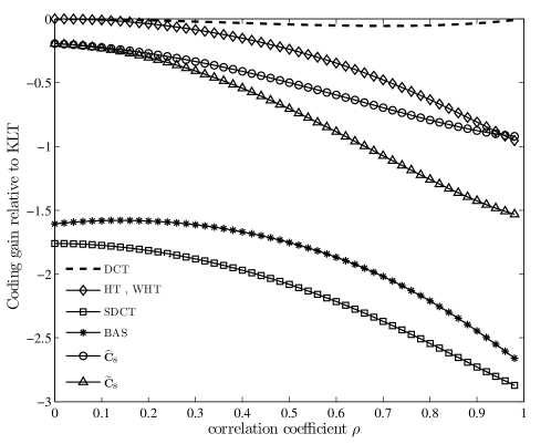
Figure 2: Coding gain relative to the KLT for the considered transforms.

Figure 2 compares the values of coding gain relative to the KLT for the considered transforms in the range $0\leq\rho<1$. As expected, the DCT has the smallest difference with respect to the KLT, followed by the HT and WHT (both with the same values). Roughly orthogonal transforms tend to show better coding gain performance when compared to nonorthogonal. The proposed transforms $\widehat{\mathbf{C}}_{8}$ and $\widetilde{\mathbf{C}}_{8}$ could outperform the SDCT and BAS, both nonorthogonal transformations. As $\rho\to 1$, the approximation $\widehat{\mathbf{C}}_{8}$ performs as well as the HT and WHT. This scenario is realistic for image compression, because natural images exhibit high inter-pixel correlation [17].

4.2 Computational cost

The low-complexity matrices associated to the proposed approximations and their inverses possess multiplierless matrix factorizations as shown in (7), (8), (9), and (10). Therefore, the only truly multiplicative elements are the ones found in the diagonal matrices $\widetilde{\mathbf{S}}_{8}$ and $\widehat{\mathbf{S}}_{8}$. However, in the context of image and video coding, such diagonal matrices can easily absorbed in the quantization step [3, 9, 31, 14]. As a consequence, in that context, the introduced approximations can be understood as fully multiplierless operations.

Table 2 presents the arithmetic complexity of the considered transforms. The computational cost of the exact DCT according to the Chen’s factorization (cf. (3)) [12] and the integer DCT for HEVC [34] are also included for comparison. The proposed approximation $\widehat{\mathbf{C}}_{8}$ requires only 22 additions. On the other hand, the computational cost of $\widetilde{\mathbf{C}}_{8}$ is comparatively larger.

Table 2: Arithmetic complexity of the considered 8-point transforms

Transform	Mult	Add	Shift	Total
DCT [12]	$16$	$26$	$0$	$42$
HEVC [34]	$0$	$50$	$30$	$80$
$\widehat{\mathbf{C}}_{8}$	$0$	$22$	$0$	$22$
$\widetilde{\mathbf{C}}_{8}$	$0$	$26$	$0$	$26$
SDCT [20]	$0$	$24$	$0$	$24$
BAS [7]	$0$	$21$	$0$	$21$
WHT [23]	$0$	$24$	$0$	$24$
HT [42]	$0$	$24$	$0$	$24$

5 Low-complexity image compression

In this section, we describe a JPEG-like image compression computational experiment. Proposed transformations are evaluated in terms of their data compression capability.

5.1 JPEG-like compression

We considered a set of 30 standard 8-bit 512512 gray scale images obtained from [1]. The images were subdivided into 88 blocks. Each block $\mathbf{A}$ was submitted to the 2-D transformation given by [44]:

$$\hat{\mathbf{B}}=\hat{\mathbf{C}}\,\mathbf{A}\,\hat{\mathbf{C}}^{-1},$$

where $\hat{\mathbf{C}}$ is a particular transformation. The 64 obtained coefficients in $\hat{\mathbf{B}}$ were arranged according to the standard zig-zag sequence [46]. The first $r$ coefficients were retained, being the remaining coefficients discarded. We adopted $1\leq r\leq 45$. Then for each block $\hat{\mathbf{B}}$, the 2-D inverse transform was applied to reconstruct the compressed image:

$$\hat{\mathbf{A}}=\hat{\mathbf{C}}^{-1}\,\hat{\mathbf{B}}\,\hat{\mathbf{C}}.$$

Finally, the resulting image was compared with the original image according to the peak signal-to-noise ratio (PSNR) [24] and the structural similarity index (SSIM) [50, 49]. The absolute percentage error (APE) for such metrics relative to the exact DCT was also considered. The PSNR is the most commonly used measure for image quality evaluation. However, the SSIM measure consider visual human system characteristics which are not considered by PSNR [50]. Following the methodology proposed in [14], the average values of the measures over the 30 standard images were computed. It leads to statistically more robust results when compared with single image analysis [30].

5.2 Results

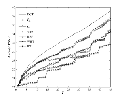
(a) Average PSNR

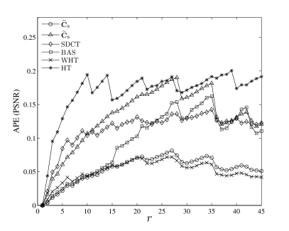
(b) Average PSNR absolute percentage error relative to the DCT.

Figure 3: PSNR measures for several compression ratios.

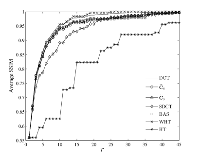
(a) Average SSIM

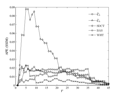
(b) Average SSIM absolute percentage error relative to the DCT

Figure 4: SSIM measures for several compression ratios.

Results of the still image compression experiment are presented in Figure 4 and 4. In Figure 4(b), the curve corresponding to the HT was suppressed because it presents excessively high values in comparison with other curves. In terms of PSNR, $\widehat{\mathbf{C}}_{8}$ outperforms both the SDCT and the BAS approximations; and provides similar results as to those furnished by the WHT, but at a lower computational cost. For SSIM results, both transforms $\widetilde{\mathbf{C}}_{8}$ and $\widehat{\mathbf{C}}_{8}$ show similar results. In terms of PSNR, the proposed approximation $\widehat{\mathbf{C}}_{8}$ performs closely to the WHT. Figure 3(a) and 3(b) show that $\widehat{\mathbf{C}}_{8}$ is superior to the WHT at high compression ratios ($r\leq 15$).

A qualitative analysis is displayed in Figure 5. Standard Elaine image was compressed and reconstructed according to the SDCT, WHT, HT, BAS, and the proposed approximation $\widehat{\mathbf{C}}_{8}$ for visual inspection. Compressed image resulted from the exact DCT is also exhibited. All images were compressed with $r=6$, which represents a removal of approximately $90.6\%$ of the transformed coefficients. The visual analysis of the obtained images shows the superiority of the proposed transform $\widehat{\mathbf{C}}_{8}$ over the SDCT in image compression. Furthermore, Table 3 lists the PSNR and SSIM values for the Elaine image, for $r=6$. The PSNR and SSIM values are listed for two additional images (Lenna and Boat images). The proposed transform $\widehat{\mathbf{C}}_{8}$ outperforms the HT, WHT, and SDCT approximations in terms of PSNR and SSIM and BAS approximation in terms of PSNR for the Elaine and Lenna images.

(a) DCT

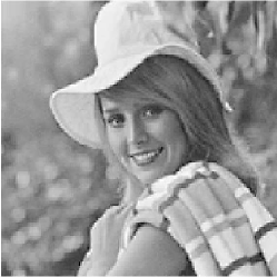
(b) SDCT

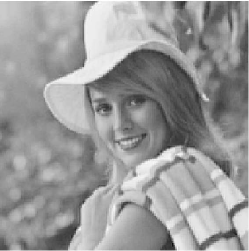
(c) WHT

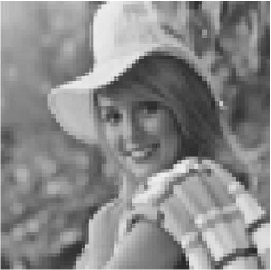
(d) HT

(e) BAS

(f) $\widehat{\mathbf{C}}_{8}$

Figure 5: Elaine image ($r=6$): 5(a) DCT, 5(b) SDCT, 5(c) WHT, 5(d) HT, 5(e) BAS and 5(f) $\widehat{\mathbf{C}}_{8}$.

Table 3: Quality measures for three compressed images, considering $r=6$

	Elaine image		Lenna image		Boat image
Transform	PSNR	SSIM	PSNR	SSIM	PSNR	SSIM
DCT [12]	$31.03$	$0.95$	$29.90$	$0.95$	$26.94$	$0.92$
$\widehat{\mathbf{C}}_{8}$	$30.00$	$0.94$	$28.79$	$0.94$	$26.04$	$0.91$
BAS [7]	$29.45$	$0.94$	$28.28$	$0.95$	$26.13$	$0.92$
WHT [23]	$28.91$	$0.92$	$27.93$	$0.92$	$25.85$	$0.90$
SDCT [20]	$27.59$	$0.88$	$26.26$	$0.88$	$24.09$	$0.85$
HT [42]	$25.44$	$0.77$	$24.27$	$0.75$	$24.27$	$0.68$

5.3 Blocking artifact analysis

A visually undesirable effect in image compression is the emergence of blocking artifacts [17, p. 573]. Figure 6 shows a qualitative comparison in terms of blocking artifact resulted from $\widehat{\mathbf{C}}_{8}$, WHT, and BAS. The proposed approximation $\widehat{\mathbf{C}}_{8}$ effected a lower degree of blocking artifact comparatively with the WHT and BAS.

(a) WHT

(b) BAS

(c) $\widehat{\mathbf{C}}_{8}$

Figure 6: Blocking artifact effect in the Elaine image ($r=6$): 6(a) WHT, 6(b) BAS and 6(c) $\widehat{\mathbf{C}}_{8}$.

6 HEVC-compliant video encoding

In this section, we aim at demonstrating the practical real-world applicability of the proposed DCT approximations for video coding. However, the HEVC standard requires not only an 8-point transform, but also 4-, 16-, and 32-point transforms. In order to derive Chen’s DCT approximations for larger blocklengths, we considered the algorithm proposed by Jridi-Alfalou-Meher (JAM) [29]. We embedded these low-complexity transforms into a publicly available reference software compliant with the HEVC standard [28].

The JAM algorithm consists of a scalable method for obtaining higher order transforms from an 8-point DCT approximation. An $N$-point DCT approximation $\check{\mathbf{T}}_{N}$, where $N$ is a power of two, is recursively obtained through:

$$\check{\mathbf{T}}_{N}=\frac{1}{\sqrt{2}}\mathbf{M}^{\text{per}}_{N}\begin{bmatrix}\check{\mathbf{T}}_{\frac{N}{2}}&\mathbf{0}_{\frac{N}{2}}\\ \mathbf{0}_{\frac{N}{2}}&\check{\mathbf{T}}_{\frac{N}{2}}\end{bmatrix}\mathbf{M}^{\text{add}}_{N},$$

where

$$\mathbf{M}^{\text{add}}_{N}=\begin{bmatrix}\mathbf{I}_{\frac{N}{2}}&\mathbf{\bar{I}}_{\frac{N}{2}}\\ \mathbf{\bar{I}}_{\frac{N}{2}}&-\mathbf{I}_{\frac{N}{2}}\end{bmatrix}\quad\text{ and }\quad\mathbf{M}^{\text{per}}_{N}=\begin{bmatrix}\mathbf{P}_{N-1,\frac{N}{2}}&\mathbf{0}_{1,\frac{N}{2}}\\ \mathbf{0}_{1,\frac{N}{2}}&\mathbf{P}_{N-1,\frac{N}{2}}\end{bmatrix},$$

and $\mathbf{P}_{N-1,\frac{N}{2}}$ is an $(N-1)\times(N/2)$ resulting from expanding the identity matrix $\mathbf{I}_{\frac{N}{2}}$ by interlacing it with zero rows. The matrix $\mathbf{M}^{\text{per}}_{N}$ is a permutation matrix and does not introduce any arithmetic cost. Matrix $\mathbf{M}^{\text{add}}_{N}$ contributes with only $N$ additions. Furthermore, the scaling factor $1/\sqrt{2}$ can be merged into the image compression quantization step and does not contribute to the arithmetic complexity of the transform. Thus, the additive complexity of $\mathbf{\check{T}}_{N}$ is equal to twice the additive complexity of $\mathbf{\check{T}}_{\frac{N}{2}}$ plus $N$ additions [29].

6.1 Chen’s DCT approximations for large blocklengths

In its original form, the JAM algorithm employs the 8-point DCT approximation introduced in [14]. In this section, we adapt the JAM algorithm to derive DCT approximations based on Chen’s algorithm for arbitrary power-of-two ($N>8$) blocklengths. We are specially interested in 16- and 32-point low-complexity transformations for subsequent embedding into the HEVC standard. Let $N>8$ be a power of two. We introduce the Chen’s signed and rounded transformations, respectively, according to the following recursion:

$$\widetilde{\mathbf{T}}_{N}=\mathbf{M}^{\text{per}}_{N}\begin{bmatrix}\widetilde{\mathbf{T}}_{\frac{N}{2}}&\mathbf{0}_{\frac{N}{2}}\\ \mathbf{0}_{\frac{N}{2}}&\widetilde{\mathbf{T}}_{\frac{N}{2}}\end{bmatrix}\mathbf{M}^{\text{add}}_{N}\quad\text{ and }\quad\widehat{\mathbf{T}}_{N}=\mathbf{M}^{\text{per}}_{N}\begin{bmatrix}\widehat{\mathbf{T}}_{\frac{N}{2}}&\mathbf{0}_{\frac{N}{2}}\\ \mathbf{0}_{\frac{N}{2}}&\widehat{\mathbf{T}}_{\frac{N}{2}}\end{bmatrix}\mathbf{M}^{\text{add}}_{N}.$$ (12)

Based on (7) and (8), $\widetilde{\mathbf{T}}_{\frac{N}{2}}$ and $\widehat{\mathbf{T}}_{\frac{N}{2}}$ admit the following factorizations:

$$\widetilde{\mathbf{T}}_{\frac{N}{2}} =\check{\mathbf{P}}_{\frac{N}{2}}\,\mathbf{M}_{\frac{N}{2}}^{(1)}\,\,\widetilde{\mathbf{M}}_{\frac{N}{2}}^{(2)}\,\,\widetilde{\mathbf{M}}_{\frac{N}{2}}^{(3)}\,\,\widetilde{\mathbf{M}}_{\frac{N}{2}}^{(4)}\,\,\check{\mathbf{B}}_{\frac{N}{2}},$$

$$\widehat{\mathbf{T}}_{\frac{N}{2}} =\check{\mathbf{P}}_{\frac{N}{2}}\,\mathbf{M}_{\frac{N}{2}}^{(1)}\,\,\widehat{\mathbf{M}}_{\frac{N}{2}}^{(2)}\,\,\widehat{\mathbf{M}}_{\frac{N}{2}}^{(3)}\,\,\widehat{\mathbf{M}}_{\frac{N}{2}}^{(4)}\,\,\check{\mathbf{B}}_{\frac{N}{2}}.$$

Thus, applying the factorizations above in (12) and expanding them, we obtain:

$$\widetilde{\mathbf{T}}_{N} =\check{\mathbf{P}}_{N}\,\mathbf{M}_{N}^{(1)}\,\,\widetilde{\mathbf{M}}_{N}^{(2)}\,\,\widetilde{\mathbf{M}}_{N}^{(3)}\,\,\widetilde{\mathbf{M}}_{N}^{(4)}\,\,\check{\mathbf{B}}_{N},$$ (13)

$$\widehat{\mathbf{T}}_{N} =\check{\mathbf{P}}_{N}\,\mathbf{M}_{N}^{(1)}\,\,\widehat{\mathbf{M}}_{N}^{(2)}\,\,\widehat{\mathbf{M}}_{N}^{(3)}\,\,\widehat{\mathbf{M}}_{N}^{(4)}\,\,\check{\mathbf{B}}_{N},$$ (14)

where

$$\check{\mathbf{P}}_{N} =\mathbf{M}^{\text{per}}_{N}\begin{bmatrix}\check{\mathbf{P}}_{\frac{N}{2}}&\mathbf{0}_{\frac{N}{2}}\\ \mathbf{0}_{\frac{N}{2}}&\check{\mathbf{P}}_{\frac{N}{2}}\end{bmatrix},\quad\check{\mathbf{B}}_{N}=\begin{bmatrix}\check{\mathbf{B}}_{\frac{N}{2}}&\mathbf{0}_{\frac{N}{2}}\\ \mathbf{0}_{\frac{N}{2}}&\check{\mathbf{B}}_{\frac{N}{2}}\end{bmatrix}\mathbf{M}^{\text{add}}_{N},\quad\mathbf{M}_{N}^{(1)}=\begin{bmatrix}\mathbf{M}_{\frac{N}{2}}^{(1)}&\mathbf{0}_{\frac{N}{2}}\\ \mathbf{0}_{\frac{N}{2}}&\mathbf{M}_{\frac{N}{2}}^{(1)}\end{bmatrix},$$

$$\widetilde{\mathbf{M}}_{N}^{(i)} =\begin{bmatrix}\widetilde{\mathbf{M}}_{\frac{N}{2}}^{(i)}&\mathbf{0}_{\frac{N}{2}}\\ \mathbf{0}_{\frac{N}{2}}&\widetilde{\mathbf{M}}_{\frac{N}{2}}^{(i)}\end{bmatrix},\quad\widehat{\mathbf{M}}_{N}^{(i)}=\begin{bmatrix}\widehat{\mathbf{M}}_{\frac{N}{2}}^{(i)}&\mathbf{0}_{\frac{N}{2}}\\ \mathbf{0}_{\frac{N}{2}}&\widehat{\mathbf{M}}_{\frac{N}{2}}^{(i)}\end{bmatrix},\quad i=2,3,4.$$

Their inverse transformations possess the following factorizations:

$$\widetilde{\mathbf{T}}_{N}^{-1} =\frac{4}{N}\,\check{\mathbf{B}}_{N}\,\left.\widetilde{\mathbf{M}}_{N}^{(4)}\right.^{-1}\left.\widetilde{\mathbf{M}}_{N}^{(3)}\right.^{-1}\left.\widetilde{\mathbf{M}}_{N}^{(2)}\right.^{-1}\left.\mathbf{M}_{N}^{(1)}\right.\check{\mathbf{P}}_{N},$$ (15)

$$\widehat{\mathbf{T}}_{N}^{-1} =\frac{4}{N}\,\check{\mathbf{B}}_{N}\,\left.\widehat{\mathbf{M}}_{N}^{(4)}\right.^{-1}\left.\widehat{\mathbf{M}}_{N}^{(3)}\right.^{-1}\left.\widehat{\mathbf{M}}_{N}^{(2)}\right.^{-1}\left.\mathbf{M}_{N}^{(1)}\right.\check{\mathbf{P}}_{N},$$ (16)

where

$$\check{\mathbf{P}}_{N} =\begin{bmatrix}\check{\mathbf{P}}_{\frac{N}{2}}&\mathbf{0}_{\frac{N}{2}}\\ \mathbf{0}_{\frac{N}{2}}&\check{\mathbf{P}}_{\frac{N}{2}}\end{bmatrix}\left.\mathbf{M}^{\text{per}}_{N}\right.,\quad\check{\mathbf{B}}_{N}=\left.\mathbf{M}^{\text{add}}_{N}\right.\begin{bmatrix}\check{\mathbf{B}}_{\frac{N}{2}}&\mathbf{0}_{\frac{N}{2}}\\ \mathbf{0}_{\frac{N}{2}}&\check{\mathbf{B}}_{\frac{N}{2}}\end{bmatrix},\quad\left.\mathbf{M}_{N}^{(1)}\right.=\begin{bmatrix}\left.\mathbf{M}_{\frac{N}{2}}^{(1)}\right.&\mathbf{0}_{\frac{N}{2}}\\ \mathbf{0}_{\frac{N}{2}}&\left.\mathbf{M}_{\frac{N}{2}}^{(1)}\right.\end{bmatrix},$$

$$\left.\widetilde{\mathbf{M}}_{N}^{(i)}\right.^{-1} =\begin{bmatrix}\left.\widetilde{\mathbf{M}}_{\frac{N}{2}}^{(i)}\right.^{-1}&\mathbf{0}_{\frac{N}{2}}\\ \mathbf{0}_{\frac{N}{2}}&\left.\widetilde{\mathbf{M}}_{\frac{N}{2}}^{(i)}\right.^{-1}\end{bmatrix},\quad\left.\widehat{\mathbf{M}}_{N}^{(i)}\right.^{-1}=\begin{bmatrix}\left.\widehat{\mathbf{M}}_{\frac{N}{2}}^{(i)}\right.^{-1}&\mathbf{0}_{\frac{N}{2}}\\ \mathbf{0}_{\frac{N}{2}}&\left.\widehat{\mathbf{M}}_{\frac{N}{2}}^{(i)}\right.^{-1}\end{bmatrix},\quad i=2,3,4.$$

In particular, for $N=16$, we have from (7) and (8) that $\check{\mathbf{P}}_{8}=\mathbf{P}_{8}$, $\check{\mathbf{B}}_{8}=\mathbf{B}_{8}$, $\mathbf{M}_{8}^{(1)}=\mathbf{M}_{1}$, $\widetilde{\mathbf{M}}_{8}^{(i)}=\widetilde{\mathbf{M}}_{i}$, $\widehat{\mathbf{M}}_{8}^{(i)}=\widehat{\mathbf{M}}_{i}$, $i=2,3,4$, and therefore it yields:

$$\widetilde{\mathbf{T}}_{16} =\check{\mathbf{P}}_{16}\,\mathbf{M}_{16}^{(1)}\,\,\widetilde{\mathbf{M}}_{16}^{(2)}\,\,\widetilde{\mathbf{M}}_{16}^{(3)}\,\,\widetilde{\mathbf{M}}_{16}^{(4)}\,\,\check{\mathbf{B}}_{16},$$

$$\widehat{\mathbf{T}}_{16} =\check{\mathbf{P}}_{16}\,\mathbf{M}_{16}^{(1)}\,\,\widehat{\mathbf{M}}_{16}^{(2)}\,\,\widehat{\mathbf{M}}_{16}^{(3)}\,\,\widehat{\mathbf{M}}_{16}^{(4)}\,\,\check{\mathbf{B}}_{16},$$

where

$$\check{\mathbf{P}}_{16} =\mathbf{M}^{\text{per}}_{16}\begin{bmatrix}\mathbf{P}_{8}&\mathbf{0}_{8}\\ \mathbf{0}_{8}&\mathbf{P}_{8}\end{bmatrix},\quad\check{\mathbf{B}}_{16}=\begin{bmatrix}\mathbf{B}_{8}&\mathbf{0}_{8}\\ \mathbf{0}_{8}&\mathbf{B}_{8}\end{bmatrix}\mathbf{M}^{\text{add}}_{16},\quad\mathbf{M}_{16}^{(1)}=\begin{bmatrix}\mathbf{M}_{1}&\mathbf{0}_{8}\\ \mathbf{0}_{8}&\mathbf{M}_{1}\end{bmatrix},$$

$$\widetilde{\mathbf{M}}_{16}^{(i)} =\begin{bmatrix}\widetilde{\mathbf{M}}_{i}&\mathbf{0}_{8}\\ \mathbf{0}_{8}&\widetilde{\mathbf{M}}_{i}\end{bmatrix},\quad\widehat{\mathbf{M}}_{16}^{(i)}=\begin{bmatrix}\widehat{\mathbf{M}}_{i}&\mathbf{0}_{8}\\ \mathbf{0}_{8}&\widehat{\mathbf{M}}_{i}\end{bmatrix},\quad i=2,3,4.$$

The near orthogonal DCT approximations linked to the proposed low-complexity matrices are given by (cf. Section 3.1):

$$\widetilde{\mathbf{C}}_{N}=\widetilde{\mathbf{S}}_{N}\,\widetilde{\mathbf{T}}_{N},\quad\widehat{\mathbf{C}}_{N}=\widehat{\mathbf{S}}_{N}\,\widehat{\mathbf{T}}_{N},$$

where $\widetilde{\mathbf{S}}_{N}=\sqrt{[\operatorname{diag}(\widetilde{\mathbf{T}}_{N}\,\widetilde{\mathbf{T}}_{N})]^{-1}}$ and $\widehat{\mathbf{S}}_{N}=\sqrt{[\operatorname{diag}(\widehat{\mathbf{T}}_{N}\,\widehat{\mathbf{T}}_{N})]^{-1}}$.

Because the entries of $\widetilde{\mathbf{T}}_{8}$ and $\widehat{\mathbf{T}}_{8}$ and their inverses are in the set $\mathcal{P}=\{0,\pm\frac{1}{2},\pm 1,\pm 2\}$, we have that the matrices in (13), (14), (15) and (16) also have entries in $\mathcal{P}$. Moreover, (13), (14), (15) and (16) can also be recursively obtained from (7), (8), (9), and (10). Thus, $\widetilde{\mathbf{C}}_{N}$ and $\widehat{\mathbf{C}}_{N}$ are low-complexity DCT approximations for blocklength $N$. The arithmetic complexity of the proposed 16- and 32-point Chen’s approximations and transformations prescribed in the HEVC standard are presented in Table 4. In terms of hardware implementation, the circuitry corresponding to $\widetilde{\mathbf{C}}_{8}$ and $\widehat{\mathbf{C}}_{8}$ and their inverses can be re-used for the hardware implementation of both the direct and inverse Chen’s DCT approximations for larger blocklengths.

Table 4: Arithmetic complexity of the considered 16- and 32-point transforms

Transform	Mult	Add	Shift	Total
16-point exact DCT [12]	$44$	$74$	$0$	$118$
16-point transform in HEVC [34]	$0$	$186$	$86$	$272$
$\widehat{\mathbf{C}}_{16}$	$0$	$60$	$0$	$60$
$\widetilde{\mathbf{C}}_{16}$	$0$	$68$	$0$	$68$
32-point exact DCT [12]	$116$	$194$	$0$	$310$
32-point transform in HEVC [34]	$0$	$682$	$278$	$960$
$\widehat{\mathbf{C}}_{32}$	$0$	$152$	$0$	$152$
$\widetilde{\mathbf{C}}_{32}$	$0$	$168$	$0$	$168$

6.2 Results

The proposed approximations were embedded into the HEVC reference software [28]. For video coding experiments we considered two set of videos, namely: (i) Group A, which consider eleven CIF videos from [52]; (ii) Group B, with six standard video sequence, one for each class specified in the Common Test Conditions (CTC) document for HEVC [6]. Such classification is based on the resolution, frame rate and, as consequence, the main applications of these kind of media [36]. All test parameters were set according to the CTC document, including the quantization parameter (QP) that assumes values in {22, 27, 32, 37}. As suggested in [29], we selected the Main profile and All-Intra mode for our experiments.

The PSNR measurements—already furnished by the reference software—were obtained for each video frame and YUV channel. The overall PSNR was obtained from each frame according to [37]. We averaged the PSNR values for the first 100 frames of all videos in each group. Figure 7 shows the average PSNR in terms of the quantization parameter (QP) for each set of 8-, 16-, and 32-point transforms: $\widetilde{\mathbf{C}}_{N}$, $\widehat{\mathbf{C}}_{N}$, and the original transforms in the HEVC standard. Results in Figure 7 show no significant degradation in terms of PSNR regardless of the video group. The proposed approximations resulted in essentially the same frame quality while having a very low computational cost when compared to those originally employed in HEVC.

Additionally, we computed the Bjøntegaard delta PSNR (BD-PSNR) and delta rate (BD-Rate) [19, 4] for compressed videos considering all discussed 8- to 32-point transformations. The first 11 rows of Table 5 present the results for the Group A whilst the remaining ones correspond to Group B. We report a negligible impact in video quality associated to the results from the modified HEVC with the approximate transforms. Similar to the still images experiments, $\widehat{\mathbf{C}}_{N}$ performed better than $\widetilde{\mathbf{C}}_{N}$ with a degradation of no more than 0.70dB and 0.58dB for Groups A and B, respectively. These declines in PSNR represent an increase of 10.63% and 7.02% in bitrate, respectively.

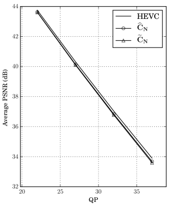
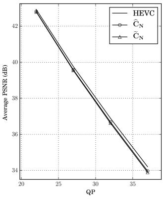
Figure 7: Average PSNR for QP in {22,27,32,37} for videos in Groups (a) A and (b) B.

Table 5: Bjøntegaard metrics for the approximate transforms and tested video sequences

Video information	BD-PSNR (dB)		BD-Rate (%)
	$\widetilde{\mathbf{C}}_{N}$	$\widehat{\mathbf{C}}_{N}$	$\widetilde{\mathbf{C}}_{N}$	$\widehat{\mathbf{C}}_{N}$
Akiyo	0.4600	0.2990	$-7.0310$	$-4.6870$
Bowing	0.5301	0.4316	$-7.4519$	$-6.1509$
Coastguard	0.7596	0.7026	$-11.3634$	$-10.6298$
Container	0.4075	0.3750	$-6.3002$	$-5.8044$
Foreman	0.2263	0.1627	$-4.4006$	$-3.2148$
Hall_monitor	0.2754	0.1952	$-4.7577$	$-3.4125$
Mobile	0.2752	0.2629	$-2.7072$	$-2.5860$
Mother_daughter	0.4202	0.3384	$-7.8362$	$-6.4112$
News	0.2539	0.1975	$-3.4211$	$-2.6772$
Pamphlet	0.4253	0.3680	$-5.8660$	$-5.1057$
Silent	0.3029	0.2399	$-5.7215$	$-4.6042$
PeopleOnStreet	0.5350	0.4734	$-9.6530$	$-8.6227$
BasketballDrive	0.3372	0.2531	$-11.7780$	$-9.0093$
RaceHorses	0.6444	0.5781	$-7.7823$	$-7.0233$
BlowingBubbles	0.2563	0.1986	$-4.3438$	$-3.4080$
KristenAndSara	0.4651	0.3807	$-8.8416$	$-7.3234$
BasketballDrillText	0.1984	0.1565	$-3.7436$	$-2.9711$

As a qualitative example, Figure 6.2 displays particular frames of Silent and PeopleOnStreet video sequences after compression according to the original HEVC and to the modified versions of HEVC based on the proposed transforms. Visual inspection shows no sign of image quality degradation.

(a) HEVC

(b) $\widetilde{\mathbf{C}}_{N}$

(d) HEVC

(e) $\widetilde{\mathbf{C}}_{N}$

(f) $\widehat{\mathbf{C}}_{N}$

Figure 8: Qualitative comparison of frames from Silent and PeopleOnStreet videos compressed with proposed Chen’s DCT approximations and default HEVC transforms and QP=32.

7 Conclusion

We introduced two new multiplierless DCT approximations based on the Chen’s factorization. The suggested approximations were assessed and compared with other well-known approximations. The proposed transformation $\widehat{\mathbf{C}}_{8}$ presented low total error energy and very close similarity to the exact DCT. Furthermore, $\widehat{\mathbf{C}}_{8}$ presents very close coding gain when compared to the optimal KLT. The approximation $\widehat{\mathbf{C}}_{8}$ outperformed the SDCT, BAS, and HT as tools for JPEG-like still image compression at a lower computational cost. Adapting the JAM scalable method, we also proposed low-complexity Chen’s DCT approximations $\widetilde{\mathbf{C}}_{N}$ and $\widehat{\mathbf{C}}_{N}$, were $N\geq 16$ is a power of two; we also provided fast algorithms for their implementations. The introduced 8-, 16-, and 32-point approximations were embedded into an HEVC reference software and assessed for video compression. Finally, the proposed low-complexity transforms are suitable for image and video coding, being a realistic alternative for efficient and low complexity image/video coding.

References

• [1] The USC-SIPI Image Database, University of Southern California, Signal and Image Processing Institute., 2011.
• [2] N. Ahmed, T. Natarajan, and K. R. Rao, Discrete Cosine Transform, IEEE Trans. Comput., C-23 (1974), pp. 90–93.
• [3] F. M. Bayer and R. J. Cintra, DCT-like transform for image compression requires 14 additions only, Electron. Lett., 48 (2012), pp. 919–921.
• [4] G. Bjøntegaard, Calculation of average PSNR differences between RD-curves, in 13th VCEG Meeting, Austin, TX, USA, Apr 2001. Document VCEG-M33.
• [5] R. E. Blahut, Fast Algorithms for Signal Processing, Cambridge University Press, 2010.
• [6] F. Bossen, Common test conditions and software reference configurations, 2013. Document JCT-VC L1100.
• [7] S. Bouguezel, M. O. Ahmad, and M. N. S. Swamy, A multiplication-free transform for image compression, in 2nd International Conference on Signals, Circuits and Syst. (SCS), Nov. 2008, pp. 1–4.
• [8]  , A novel transform for image compression, in IEEE 53rd International Midwest Symposium on Circuits Syst. (MWSCAS), Aug. 2010, pp. 509–512.
• [9]  , A low-complexity parametric transform for image compression, in IEEE International Symposium on Circuits Syst. (ISCAS), May 2011, pp. 2145–2148.
• [10] V. Britanak, P. C. Yip, and K. R. Rao, Discrete Cosine and Sine Transforms: General Properties, Fast Algorithms and Integer Approximations, Elsevier Science, 2010.
• [11] T. S. Chang, C. S. Kung, and C. W. Jen, A simple processor core design for DCT/IDCT, IEEE Trans. Circuits Syst. Video Technol., 10 (2000), pp. 439–447.
• [12] W. H. Chen, C. Smith, and S. Fralick, A fast computational algorithm for the Discrete Cosine Transform, IEEE Trans. Commun., 25 (1977), pp. 1004–1009.
• [13] R. J. Cintra, An integer approximation method for discrete sinusoidal transforms, Circuits, Syst., and Signal Process., 30 (2011), pp. 1481–1501.
• [14] R. J. Cintra and F. M. Bayer, A DCT approximation for image compression, IEEE Signal Process. Lett., 18 (2011), pp. 579–582.
• [15] M. Effros, H. Feng, and K. Zeger, Suboptimality of the Karhunen-Loève transform for transform coding, IEEE Trans. Inf. Theory, 50 (2004), pp. 1605–1619.
• [16] B. N. Flury and W. Gautschi, An algorithm for simultaneous orthogonal transformation of several positive definite symmetric matrices to nearly diagonal form, SIAM J. Sci. Stat. Comput., 7 (1986), pp. 169–184.
• [17] R. C. Gonzalez and R. E. Woods, Digital image processing, Prentice-Hall, Inc., Upper Saddle River, NJ, USA, 3rd ed., 2006.
• [18] J. Han, Y. Xu, and D. Mukherjee, A butterfly structured design of the hybrid transform coding scheme, in Picture Coding Symposium, 2013, pp. 1–4.
• [19] P. Hanhart and T. Ebrahimi, Calculation of average coding efficiency based on subjective quality scores, J. Vis. Commun. Image R., 25 (2014), pp. 555–564.
• [20] T. I. Haweel, A new square wave transform based on the DCT, Signal Process., 81 (2001), pp. 2309–2319.
• [21] N. J. Higham, Computing the polar decomposition with applications, SIAM J. Sci. Stat. Comput., 7 (1986), pp. 1160–1174.
• [22] N. J. Higham, Computing real square roots of a real matrix, Linear Algebra Appl., 88–89 (1987), pp. 405–430.
• [23] K. J. Horadam, Hadamard matrices and their applications, Cryptography Commun., 2 (2010), pp. 129–154.
• [24] Q. Huynh-Thu and M. Ghanbari, Scope of validity of PSNR in image/video quality assessment, Electron. Lett., 44 (2008), pp. 800–801.
• [25] International Organisation for Standardisation, Generic coding of moving pictures and associated audio information – Part 2: Video, ISO/IEC JTC1/SC29/WG11 - coding of moving pictures and audio, ISO, 1994.
• [26] International Telecommunication Union, ITU-T recommendation H.261 version 1: Video codec for audiovisual services at $p\times 64$ kbits, tech. rep., ITU-T, 1990.
• [27]  , ITU-T recommendation H.263 version 1: Video coding for low bit rate communication, tech. rep., ITU-T, 1995.
• [28] Joint Collaborative Team on Video Coding (JCT-VC), HEVC reference software documentation, 2013. Fraunhofer Heinrich Hertz Institute.
• [29] M. Jridi, A. Alfalou, and P. K. Meher, A generalized algorithm and reconfigurable architecture for efficient and scalable orthogonal approximation of DCT, IEEE Trans. Circuits Syst. I, Reg. Papers, 62 (2015), pp. 449–457.
• [30] S. M. Kay, Fundamentals of Statistical Signal Processing, Volume I: Estimation Theory, vol. 1 of Prentie Hall Signal Processing Series, Prentice Hall, Upper Saddle River, NJ, 1993.
• [31] K. Lengwehasatit and A. Ortega, Scalable variable complexity approximate forward DCT, IEEE Trans. Circuits Syst. Video Technol., 14 (2004), pp. 1236–1248.
• [32] J. Liang and T. D. Tran, Fast multiplierless approximations of the DCT with the lifting scheme, IEEE Trans. Signal Process., 49 (2001), pp. 3032–3044.
• [33] C. Loeffler, A. Ligtenberg, and G. S. Moschytz, Practical fast 1-D DCT algorithms with 11 multiplications, in International Conference on Acoust., Speech, Signal Process. (ICASSP), May 1989, pp. 988–991.
• [34] P. K. Meher, S. Y. Park, B. K. Mohanty, K. S. Lim, and C. Yeo, Efficient Integer DCT Architectures for HEVC, IEEE Trans. Circuits Syst. Video Technol., 24 (2014), pp. 168–178.
• [35] J. K. Merikoski, On the trace and the sum of elements of a matrix, Linear Algebra Appl., 60 (1984), pp. 177–185.
• [36] M. Naccari and M. Mrak, Chapter 5 - perceptually optimized video compression, in Academic Press Library in signal Processing Image and Video Compression and Multimedia, vol. 5, Elsevier, 2014, pp. 155–196.
• [37] J.-R. Ohm, G. J. Sullivan, H. Schwarz, T. K. Tan, and T. Wiegand, Comparison of the coding efficiency of video coding standards - including high efficiency video coding (HEVC), IEEE Trans. Circuits Syst. Video Technol., 22 (2012), pp. 1669–1684.
• [38] M. T. Pourazad, C. Doutre, M. Azimi, and P. Nasiopoulos, HEVC: The new gold standard for video compression: How does HEVC compare with H.264/AVC?, IEEE Consum. Electron. Mag., 1 (2012), pp. 36–46.
• [39] A. Puri, X. Chen, and A. Luthra, Video coding using the H.264/MPEG-4 AVC compression standard, Signal Process.: Image Commun., 19 (2004), pp. 793–849.
• [40] N. Roma and L. Sousa, Efficient hybrid DCT-domain algorithm for video spatial downscaling, EURASIP J. Adv. Signal Process, 2007 (2007), pp. 1–16.
• [41] G. A. F. Seber, A Matrix Handbook for Statisticians, John Wiley & Sons, Inc, 2008.
• [42] J. Seberry, B. J. Wysocki, and T. A. Wysocki, On some applications of Hadamard matrices, Metrika, 62 (2005), pp. 221–239.
• [43] N. Suehiro and M. Hatori, Fast algorithms for the DFT and other sinusoidal transforms, IEEE Trans. Acoust., Speech, Signal Process., 34 (1986), pp. 642–644.
• [44] T. Suzuki and M. Ikehara, Integer DCT based on direct-lifting of DCT-IDCT for lossless-to-lossy image coding, IEEE Trans. Image Process., 19 (2010), pp. 2958–2965.
• [45] C. Tablada, F. Bayer, and R. Cintra, A class of DCT approximations based on the Feig-–Winograd algorithm, Signal Process., 113 (2015), pp. 38–51.
• [46] G. Wallace, The JPEG still picture compression standard, IEEE Trans. Consum. Electron., 38 (1992), pp. 18–34.
• [47] Z. Wang, Reconsideration of: A fast computational algorithm for the Discrete Cosine Transform, IEEE Trans. Commun., 31 (1983), pp. 121–123.
• [48]  , Fast algorithms for the discrete W transform and for the Discrete Fourier Transform, IEEE Trans. Acoust., Speech, Signal Process., 32 (1984), pp. 803–816.
• [49] Z. Wang and A. C. Bovik, Mean squared error: Love it or leave it? A new look at signal fidelity measures, IEEE Signal Process. Mag., 26 (2009), pp. 98–117.
• [50] Z. Wang, A. C. Bovik, H. R. Sheikh, and E. P. Simoncelli, Image quality assessment: from error visibility to structural similarity, IEEE Trans. Image Process., 13 (2004), pp. 600–612.
• [51] D. Watkins, Fundamentals of Matrix Computations, Pure and Applied Mathematics: A Wiley Series of Texts, Monographs and Tracts, Wiley, 2004.
• [52] Xiph.Org Foundation, Xiph.org video test media, 2014.
• [53] W. Yuan, P. Hao, and C. Xu, Matrix factorization for fast DCT algorithms, in IEEE International Conference on Acoust., Speech, Signal Process. (ICASSP), vol. 3, May 2006, pp. 948–951.