]sites.google.com/a/alaska.edu/chungsangng/

A “Galactic Disk”-Model for Three-Dimensional Bernstein-Greene-Kruskal Modes in a Finite Magnetic Field

Abstract

A new model, inspired by the structure of galactic disks, for three-dimensional Bernstein-Greene-Kruskal (BGK) modes in a plasma with a uniform finite background magnetic field is presented. These modes are exact nonlinear solutions of the steady-state Vlasov equation, with an electric potential and a magnetic potential perturbation localized in all three spatial dimensions that satisfies the Poisson equation, and the Ampère Law, self-consistently. The existence of solutions is shown analytically in the limit of small electric and magnetic field perturbations associated with the disk species, and numerically using an iterative method that converges up to moderately strong field perturbations.

Introduction.— A fundamental problem in plasma physics is whether small kinetic scale structures can form in high temperature collisionless plasmas. One possible solution for such structures was obtained by Bernstein, Greene, and Kruskal, known as the BGK mode [1]. The original BGK mode is a one-dimensional (1D) steady-state solution of the Vlasov-Poisson system of equations, which means the solution depends on one Cartesian coordinate such that the electric potential for a localized solution tends to zero as this coordinate tends to $\pm\infty$. There have been a large volume of research on BGK modes than we can cite here in a short paper. A more comprehensive discussion on relevant literature can be found in our recent paper [2], as well as a recent review paper [3]. Here we restrict our discussion on three-dimensional (3D) BGK modes, which have a localized electric potential that tends to zero along any direction in a 3D spatial space. Motivated by multi-dimensional features observed in space plasmas [4], a theory of 3D BGK modes was developed in a plasma within a uniform magnetic field with infinite field strength [5, 6, 7], which has been further developed recently [8]. The original theory has imposed a cylindrical symmetry, mainly for convenience, so the solution depends on two coordinates. It is considered 3D since the electric potential is localized in the sense mentioned above. In the other extreme in the parameter space, another 3D BGK mode was found in an unmagnetized (zero magnetic field) plasma [9]. That mode is still considered 3D despite having spherical symmetry such that the solution depends only on the spherical radial coordinate, because the electric potential tends to zero along all radial directions within a 3D spatial space. The physical mechanism for this mode is different from other solutions discussed so far, since it is not based on particle trapping. Instead, it is due to the dependence on another conserved quantity, the angular momentum associated with the spherical symmetry, in addition to the energy in the particle distribution function. For a magnetic field with a finite field strength, in between the above two extremes, no exact 3D BGK mode solutions are found so far. However, a theory of 2D BGK modes under this condition was developed [10], with the distribution function depending also on the canonical angular momentum, which was later developed further [2], with the additional dependence on the canonical momentum along the direction of the background magnetic field. These solutions are considered 2D since the localized electric potential tends to zero along any directions on a 2D plane perpendicular to the magnetic field direction, despite depending only on the spatial cylindrical radial coordinate after imposing the cylindrical symmetry.

The kinetic theory of a plasma turns out to be formally very similar to that of galactic dynamics such that “many of the mathematical tools that have been developed to study stellar systems are borrowed from plasma physics” [11]. In the linear regime, fundamental concepts like Landau damping and Case-Van Kampen modes are also very relevant to waves and instabilities within a stellar system [12]. In the nonlinear regime, a stellar equilibrium, such as a galaxy, can be obtained theoretically using a mathematical framework similar to constructing a 3D BGK mode [9]. One major difference between the two systems is that the gravitational interaction between stars is always attractive, while the electric force is repulsive between charges of the same sign. Because of this difference, finding an equilibrium solution for a stellar system turns out to be much easier than for a plasma.

In the development of a theory of 3D BGK modes for a magnetized plasma with a finite field strength, the direction of the influence of ideas is reversed here. Our new model is inspired by the existence of disk galaxies, one of the most magnificent structures in the universe that can be easily observed. In this “Galactic Disk”-model, the BGK mode is supported by introducing a localized disk species that is also spinning (due to the dependence of the canonical angular momentum in the distribution function of the disk species), similar to a disk galaxy (although without spiral arms due to the imposed cylindrical symmetry). In the following, we first present the mathematical formulation of this model, showing analytically the existence of solutions in the limit of weak electric and magnetic field perturbations associated with the disk. We then present numerical solutions beyond this limit, using an iteration scheme that converges up to a case with moderately large electric and magnetic field perturbations. Possible implications of the new models are then discussed, with the interesting possibility that the existence of disk-like structures in a plasma might provide insights to fundamental problems in galactic dynamics.

A “Galactic Disk”-Model.— We start the construction of 3D BGK modes by requiring the distribution function $f_{s}$ for species $s$ to be a time-steady solution satisfying the Vlasov (Collisionless Boltzmann) equations,

$$\frac{\partial f_{s}}{\partial t}+\textbf{v}\cdot\frac{\partial f_{s}}{\partial\textbf{r}}+\frac{q_{s}}{m_{s}}(\textbf{E}+\textbf{v}\times\textbf{B})\cdot\frac{\partial f_{s}}{\partial\textbf{v}}=0\;,$$ (1)

where $q_{s}$ and $m_{s}$ are the charge and mass of the $s$ particle, with $f_{s}$ assumed to be independent of time $t$ so that $f_{s}=f_{s}(\textbf{r},\textbf{v})$ depends only on spatial and velocity space independent variables r and v. While generally we can have as many $s$ species as we want, we will for simplicity restrict our study here to $s=i$, $e$, $d$, for the three species, ions, electrons, and the “disk” particles. In the numerical examples presented in this paper, we will further choose ions to be protons, and the $d$ particles to be another population of electrons, distinguished from the main $e$ species. Under this choice, we have $m_{i}=m_{p}$, the proton mass, $m_{d}=m_{e}$, the electron mass, and $q_{i}=e>0$, $q_{e}=q_{d}=-e$ with $e$ being the magnitude of the electron charge. For general expressions, it is convenient to define $M_{s}=m_{s}/m_{e}$, and $Z_{s}=q_{s}/e$. The electric field $\textbf{E}=-\nabla\psi$ and the magnetic field $\textbf{B}=\nabla\times\textbf{A}$ in Eq. (1), or the electric potential $\psi$ and the magnetic potential A, are related self-consistently and nonlinearly with $f_{s}$ through the Gauss Law (Poisson equation) and the Ampère Law,

$$\nabla^{2}\psi=-\frac{\rho_{q}}{\epsilon_{0}} = -\frac{1}{\epsilon_{0}}\sum_{s}q_{s}\int d^{3}vf_{s}\;,$$ (2)

$$\nabla\times\nabla\times\textbf{A}=\mu_{0}\textbf{J} = \mu_{0}\sum_{s}q_{s}\int d^{3}vf_{s}\textbf{v}\;.$$ (3)

We are looking for localized 3D BGK modes in a magnetic field $\textbf{B}=B_{\infty}\hat{z}$, and a uniform background plasma with Maxwellian electrons and ions with density $n_{e0}$ and $n_{i0}=n_{e0}/Z_{i}$, and temperature $T_{e0}$ and $T_{i0}$ respectively. Therefore, we impose boundary conditions for $\psi$ and the magnetic potential perturbation $\textbf{a}=\textbf{A}-0.5B_{\infty}\rho\hat{\phi}$ that they tend to zero as $|\textbf{r}|\rightarrow\infty$ along any direction in a 3D spatial space. Note that we are using a cylindrical coordinate system with coordinates $\rho$, $\phi$, $z$ and corresponding unit vectors $\hat{\rho}$, $\hat{\phi}$, $\hat{z}$. The origin of the coordinate system is chosen to be the center of the mode structure. To simplify expressions, from now on we will normalize our equations using the electron thermal velocity $v_{e}=(k_{B}T_{e0}/m_{e})^{1/2}$ as the unit for v, with $k_{B}$ being the Boltzmann constant and $T_{e0}$ the background electron temperature, the electron Debye length $\lambda_{D}=v_{e}/\omega_{pe}=v_{e}(\epsilon_{0}m_{e}/n_{e0})^{1/2}/e$ as the unit for r, $n_{e0}e\lambda^{2}_{D}/\epsilon_{0}$ as the unit for $\psi$, $n_{e0}e\lambda_{D}/\epsilon_{0}v_{e}$ as the unit for B, $n_{e0}/v^{3}_{e}$ as the unit for $f_{e}$, and $n_{i0}/v^{3}_{e}$ as the unit for $f_{i}$.

To look for time steady solutions of Eq. (1) for $f_{s}$, it is well known that we can simply require $f_{s}$ to depend only on conserved quantities. One obvious conserved quantity is the total (kinetic plus electrostatic potential) particle energy with a normalized form proportional to $w_{s}=v^{2}/2+\zeta_{s}\psi$, with $\zeta_{s}=Z_{s}/M_{s}$. To make use of another conserved quantity, we need to impose a cylindrical symmetry such that physical quantities do not depend on $\phi$. With this symmetry, another conserved quantity is the $z$-component of the canonical angular momentum, with a normalized form proportional to $l_{s}=2\rho(v_{\phi}+\zeta_{s}A_{\phi})$, where the subscript $\phi$ indicates the $\phi$-component. Note that in the theory of 2D BGK modes [10, 2], with solutions also independent of $z$, there is another conserved quantity, i.e., the $z$-component of the canonical momentum, with a normalized form proportional to $v_{z}+\zeta_{s}A_{z}$. For the 3D case, with one less conserved quantity, the task of finding a solution satisfying Eqs. (2) and (3) becomes much more difficult. In the theory of 3D BGK modes in the limit of an infinitely strong background magnetic field [5, 6, 7], another conserved quantity is simply the radial coordinate $\rho$, since charged particles move only along the background magnetic field lines under this assumption. To obtain a solution without the drastic assumption of infinite magnetic field strength, it would be very helpful to make use of another conserved quantity. Inspired by the dynamics of galaxies, a dynamical system closely related to the Vlasov system considered here, we will employ the non-classical integral of motion (or the third integral) that allows the existence of thin galactic disks (see Section 4.5 of Ref. [11]). In contrast with classical integrals of motions $w_{s}$ and $l_{s}$ discussed above, non-classical integrals of motion cannot be expressed as functions of coordinates of the phase space. Instead, they are expressed as a restriction of particle motions. We impose this particular non-classical integral of motion by introducing a disk species with a normalized distribution

$$f_{d}=\frac{h_{d}}{2\pi\tau_{d}}\delta\left(v_{z}\right)\delta\left(z\right)e^{-k_{d}l_{d}-w_{d}/\tau_{d}}\;,$$ (4)

where $w_{d}$ and $l_{d}$ are defined as above with $s=d$, $\tau_{d}=v^{2}_{d}/v^{2}_{e}$ with $v_{d}$ being the thermal velocity of the particles of the disk species, $k_{d}$ and $h_{d}$ are constants. Moreover, for a localized disk with $f_{d}\rightarrow 0$ as $\rho\rightarrow\infty$, the asymptotic magnetic field strength has to satisfy $B_{\infty}>2k_{d}\tau_{d}/\zeta_{d}>0$. One can check that the form of $f_{d}$ in Eq. (4) satisfies the Vlasov equation, Eq. (1), if $\psi$ and A have the cylindrical symmetry, as well as a reflection symmetry with respect to the $z=0$ plane, i.e.,

$$\psi\left(\rho,-z\right)=\psi\left(\rho,z\right),\,A_{\phi}\left(\rho,-z\right)=A_{\phi}\left(\rho,z\right)\;,$$ (5)

with $\textbf{A}=A_{\phi}(\rho,z)\hat{\phi}$, such that on the $z=0$ plane $\textbf{E}=E_{\rho}(\rho)\hat{\rho}$ and $\textbf{B}=B_{z}(\rho)\hat{z}$. Therefore, all disk particles will stay on the $z=0$ plane, because their velocity and acceleration vectors are also on the same plane. The dependence on $w_{d}$ and $l_{d}$ can be more general than in Eq. (4). The present form is chosen for simplicity so that the moments from $f_{d}$ can be integrated into simple analytic expressions. The disk species is also the first attempt to use a non-classical integral of motion that is most easily incorporated into the form of $f_{d}$. Results from the current work thus suggest the possibility to employ other non-classical integrals of motion as well, although doing so might be significantly more difficult.

The ion and electron distribution functions, $f_{i}$ and $f_{e}$ can also be chosen as rather general functions of $w_{s}$ and $l_{s}$. For simplicity, we set them in this paper to be Boltzmann distributions

$$f_{e}=e^{-w_{e}}/\left(2\pi\right)^{3/2},\,f_{i}=e^{-w_{i}/\tau_{i}}/\left(2\pi\tau_{i}\right)^{3/2}\;,$$ (6)

where $\tau_{i}=v^{2}_{i}/v^{2}_{e}$ with $v_{i}$ being the ion thermal velocity. The normalized charge density $\rho_{q}$ from Eqs. (4) and (6) is then

$$\rho_{q}=e^{-\zeta_{i}\psi/\tau_{i}}-e^{\psi}+\sigma\delta\left(z\right)\;,$$ (7)

where $\sigma$ is a surface charge density on the $z=0$ plane,

$$\sigma(\rho)=Z_{d}h_{d}e^{-2k_{d}\rho\left(\zeta_{d}A_{\phi}-k_{d}\tau_{d}\rho\right)-\zeta_{d}\psi/\tau_{d}}\;.$$ (8)

Similarly, because the disk has a rotational flow in the $\phi$-direction, there is a normalized current density $\textbf{J}=\nabla\times\mathbf{B}=-\xi(\rho)\delta(z)\hat{\phi}$, which is totally a surface current density, with

$$\xi(\rho)=2\beta_{d}^{2}k_{d}\rho Z_{d}h_{d}e^{-2k_{d}\rho\left(\zeta_{d}A_{\phi}-k_{d}\tau_{d}\rho\right)-\zeta_{d}\psi/\tau_{d}}\;,$$ (9)

where $\beta_{d}=v_{d}/c$ with $c$ being the speed of light in vacuum. With the charge density given by Eq. (7), the normalized form of Eq. (2) can be written as

$$\frac{\partial}{\rho\partial\rho}\left(\rho\frac{\partial\psi}{\partial\rho}\right)+\frac{\partial^{2}\psi}{\partial z^{2}}=e^{\psi}-e^{-\zeta_{i}\psi/\tau_{i}}\;,$$ (10)

for $z>0$ with $\psi\left(\rho,0\right)=\psi\left(\rho,z\rightarrow 0\right)$ and the symmetry condition Eq. (5), subject to boundary conditions $\psi\left(\rho\rightarrow\infty,z\right)\rightarrow 0$, $\psi\left(\rho,z\rightarrow\infty\right)\rightarrow 0$, as well as

$$\frac{\partial\psi\left(\rho,0^{+}\right)}{\partial z}=-\sigma\left(\rho;\psi,a_{\phi}\right)/2,\;\frac{\partial\psi\left(0,z\right)}{\partial\rho}=0\;,$$ (11)

where the semicolon notation in $\sigma$ is to indicate that it depends on $\psi$ and $a_{\phi}$ also, with $a_{\phi}=A_{\phi}-B_{\infty}\rho/2$,. Similarly, the normalized form of Eq. (3) can be written as

$$\frac{\partial^{2}a_{\phi}}{\partial\rho^{2}}+\frac{1}{\rho}\frac{{\partial a}_{\phi}}{\partial\rho}-\frac{a_{\phi}}{\rho^{2}}+\frac{\partial^{2}a_{\phi}}{\partial z^{2}}=0\;,$$ (12)

for $z>0$ with $a_{\phi}\left(\rho,0\right)=a_{\phi}\left(\rho,z\rightarrow 0\right)$ and the symmetry condition Eq. (5), subject to boundary conditions $a_{\phi}\left(\rho\rightarrow\infty,z\right)\rightarrow 0$, $a_{\phi}\left(\rho,z\rightarrow\infty\right)\rightarrow 0$, as well as

$$\frac{\partial a_{\phi}\left(\rho,0^{+}\right)}{\partial z}=\xi\left(\rho;\psi,a_{\phi}\right)/2,\;a_{\phi}\left(\rho\rightarrow 0,z\right)\rightarrow 0\;.$$ (13)

Eqs. (10) to (13) thus formulate a set of nonlinear partial differential equations for the two functions $\psi(\rho,z)$ and $a_{\phi}(\rho,z)$. Due to the complicated structure, it is likely that solutions can only be found numerically. While there can be many different numerical schemes for this problem, here we will only present a straightforward one by using Hankel transforms

$$\psi\left(\rho,z\right) = \int_{0}^{\infty}kdk\widetilde{\psi}\left(k,z\right)J_{0}\left(k\rho\right),\;$$

$$a_{\phi}\left(\rho,z\right) = \int_{0}^{\infty}kdk{\widetilde{a}}_{\phi}\left(k,z\right)J_{1}\left(k\rho\right)\;,$$ (14)

where $J_{0}$ and $J_{1}$ are Bessel functions of zeroth and first order respectively. Eqs. (10) and (11) can then be written as

$$\frac{\partial^{2}\widetilde{\psi}\left(k,z\right)}{\partial z^{2}}-\left(k^{2}+1+\frac{\zeta_{i}}{\tau_{i}}\right)\widetilde{\psi}\left(k,z\right)=-\gamma\left(k,z\right)\;,$$ (15)

where $\gamma\left(k,z\right)=\int_{0}^{\infty}{\rho d\rho\Gamma(\rho,z)J_{0}\left(k\rho\right)}$, with $\Gamma\left(\rho,z\right)=\exp({-\zeta}_{i}\psi/\tau_{i})-\exp(\psi)+\left(1+\zeta_{i}/\tau_{i}\right)\psi$, subject to the Neumann boundary condition on the $z=0$ plane

$$\frac{\partial\widetilde{\psi}\left(k,0^{+}\right)}{\partial z}=-\frac{1}{2}\int_{0}^{\infty}{\rho d\rho\sigma\left(\rho;\psi,a_{\phi}\right)J_{0}\left(k\rho\right)}\;.$$ (16)

Since $\gamma\left(k,z\rightarrow\infty\right)\rightarrow 0$, the solution $\widetilde{\psi}\propto\exp\left[-\left(k^{2}+1+\zeta_{i}/\tau_{i}\right)^{1/2}z\right]$ will be chosen for Eq. (15) in the $z\rightarrow\infty$ limit, in order to satisfy the boundary condition $\psi\left(\rho,z\rightarrow\infty\right)\rightarrow 0$. Similarly, Eqs. (12) and (13) become ${\widetilde{a}}_{\phi}\left(k,z\right)={\widetilde{a}}_{\phi}\left(k,0\right)\exp\left(-kz\right)$, with

$${\widetilde{a}}_{\phi}\left(k,0\right)=-\frac{1}{2k}\int_{0}^{\infty}{\rho d\rho\xi\left(\rho;\psi,a_{\phi}\right)J_{1}\left(k\rho\right)}\;.$$ (17)

By employing Hankel transforms, we therefore reduce the partial differential operator in Eq. (10) to an ordinary differential operator in Eq. (15), but pay the price of making it also an integral equation through the right-hand-sides of Eqs. (15) to (17). There is also an advantage that all boundary conditions can now be satisfied in a straightforward manner. Moreover, this formulation allows us to write down the solution in the weak field limit in closed form. From Eqs. (8) and (9) we see that in the limit of $h_{d}\rightarrow 0$, both the surface charge density and surface current density tend to zero. We should then expect $\psi\rightarrow\psi_{0}=0$, and $a_{\phi}\rightarrow a_{\phi 0}=0$ such that $A_{\phi}\rightarrow A_{\phi 0}=B_{\infty}\rho/2$. The right-hand-sides of Eqs. (16) and (17) no longer depend on $\psi$ and $a_{\phi}$ if we set $\sigma\left(\rho;\psi,a_{\phi}\right)\rightarrow\sigma\left(\rho;\psi_{0},a_{\phi 0}\right)=Z_{d}h_{d}\exp\left[-k_{d}\left(\zeta_{d}B_{\infty}-2k_{d}\tau_{d}\right)\rho^{2}\right]$, and $\xi\left(\rho;\psi,a_{\phi}\right)\rightarrow\xi\left(\rho;\psi_{0},a_{\phi 0}\right)=2\beta_{d}^{2}k_{d}\rho Z_{d}h_{d}\exp\left[-k_{d}\left(\zeta_{d}B_{\infty}-2k_{d}\tau_{d}\right)\rho^{2}\right]$. In the same way, the right-hand-side of Eq. (15) becomes zero because $\Gamma\rightarrow O(\psi_{0}^{2})\rightarrow 0$. The solutions for $\psi(\rho,z)$ and $a_{\phi}(\rho,z)$ in the limit of $h_{d}\rightarrow 0$ can then be solved analytically as integrals of the forms of

$$\psi\left(\rho,z\right) = \frac{Z_{d}h_{d}}{4k_{d}\left(\zeta_{d}B_{\infty}-2k_{d}\tau_{d}\right)}\int_{0}^{\infty}\frac{kdkJ_{0}\left(k\rho\right)}{\sqrt{k^{2}+1+\frac{\zeta_{i}}{\tau_{i}}}}$$ (18)

$$e^{\frac{-k^{2}}{4k_{d}\left(\zeta_{d}B_{\infty}-2k_{d}\tau_{d}\right)}-|z|\sqrt{k^{2}+1+\frac{\zeta_{i}}{\tau_{i}}}}\;,$$

$$a_{\phi}\left(\rho,z\right) = \frac{-\beta_{d}^{2}k_{d}Z_{d}h_{d}}{\left[2k_{d}\left(\zeta_{d}B_{\infty}-2k_{d}\tau_{d}\right)\right]^{2}}\int_{0}^{\infty}kdkJ_{1}\left(k\rho\right)$$ (19)

$$e^{\frac{-k^{2}}{4k_{d}\left(\zeta_{d}B_{\infty}-2k_{d}\tau_{d}\right)}-k|z|}\;.$$

It is straightforward to verify that the integrals in Eqs. (18) and (19) are well behaved such that 3D BGK solutions do exist in the weak field limit $h_{d}\rightarrow 0$. To show the existence of solutions for a finite $h_{d}$, one can try putting solutions from Eqs. (18) and (19) back into the right-hand-sides of Eqs. (15) to (17) and then solve Eq. (15) numerically in a straightforward manner, because the equation becomes an linear ODE for a new $\widetilde{\psi}$ after using the old $\psi$ and $a_{\phi}$ on the right-hand-side. The new solutions for $\psi(\rho,z)$ and $a_{\phi}(\rho,z)$ can then be put back to the iteration scheme to improve the solutions until they converge. In the following, we present one example to show that this iteration scheme does result in converged solutions up to a rather large $h_{d}$.

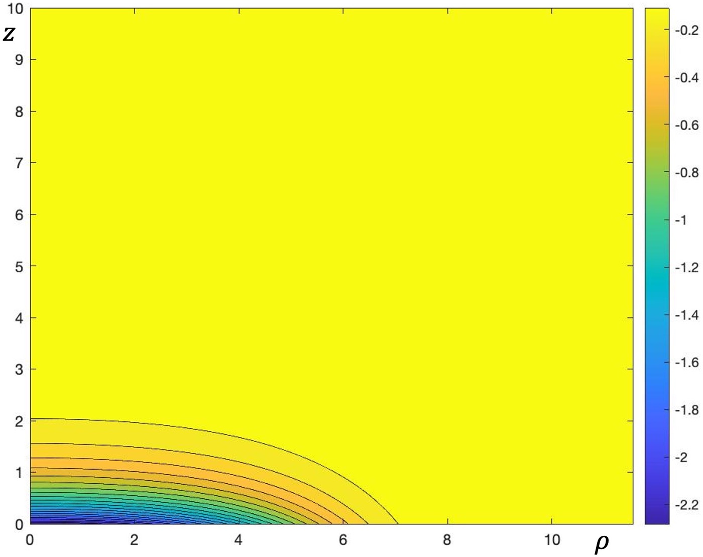
Figure 1: Color coded contour plot of the electric potential $\psi(\rho,z)$ solved from a run with $B_{\infty}=1$, $\zeta_{i}=\tau_{i}=1/1836$, $\zeta_{d}=Z_{d}=-1$, $\beta_{d}^{2}=0.01$, $\tau_{d}=1$, $k_{d}=-0.3$, and $h_{d}=79$.

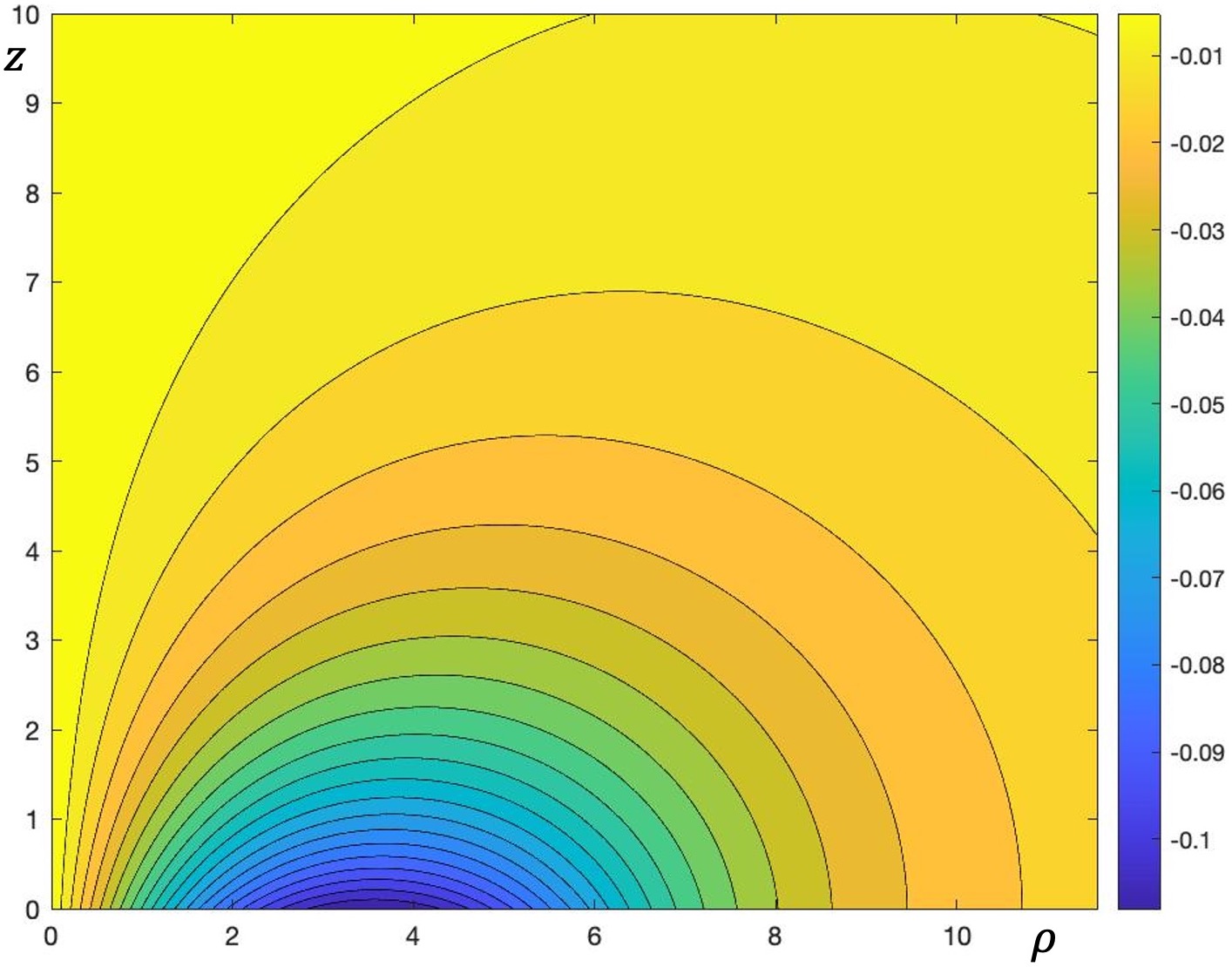
Figure 2: Color coded contour plot of the magnetic potential perturbation $a_{\phi}(\rho,z)$ solved from the same run for Fig. 1.

Numerical Solutions.— Numerical solutions $\psi(\rho,z)$ and $a_{\phi}(\rho,z)$ for Eqs. (14) to (17) are calculated on a uniform grid over a domain $\rho=(0,\rho_{max})$, and $z=(0,z_{max})$. The domain is chosen such that $\psi(\rho,z)$ and $a_{\phi}(\rho,z)$ are expected to be small for $\rho>\rho_{max}$, and $z>z_{max}$. Direct and inverse Hankel transforms are performed using numerical functions for $J_{0}$ and $J_{1}$, and integrated using an extended trapezoidal rule [13]. Because the main goal of this study is to show the existence of solutions, we have chosen to use simple straightforward numerical methods so that results can be easily verified. Therefore, we have not employed a fast Hankel transform method, which would require other more complicated numerical implementation such as a nonuniform grid. However, such a method to increase numerical efficiency can certainly be included in the future development of the code. We have confirmed the accuracy of our method in performing Hankel transforms, by comparing an analytical test function with itself after a pair of direct and inverse transforms. Eq. (15), with the boundary condition Eq. (16), is solved numerically as a linear ODE, with the right-hand-sides treated as known terms, using a second order finite difference discretization solved by a tridiagonal matrix method [14], to make sure that $\widetilde{\psi}$ is on a branch that is exponentially small for large $z$.

As outlined briefly above, the iteration scheme starts with setting $\psi=\psi_{i}$ and $a_{\phi}=a_{\phi i}$ on the right-hand-sides of Eqs. (15) to (17). New solutions $\psi=\psi_{f}$ and $a_{\phi}=a_{\phi f}$ are then solved by the method described above on the uniform grid. The convergency of solutions is tested by calculating a deviation parameter

$$d=\left[\frac{2\left<\left(\psi_{f}-\psi_{i}\right)^{2}\right>}{\left<\psi_{f}^{2}\right>+\left<\psi_{i}^{2}\right>}\right]^{1/2}+\left[\frac{2\left<\left(a_{\phi f}-a_{\phi i}\right)^{2}\right>}{\left<a_{\phi f}^{2}\right>+\left<a_{\phi i}^{2}\right>}\right]^{1/2}\;,$$ (20)

as a measure of the fractional difference between the old and new solutions, where the notation $\left<\dots\right>$ indicates a sum over all grid points of the quantity within the angle brackets. Obviously, the method converges if $d=0$. For a finite $d$, one then set $\psi_{i}=\psi_{f}$ and $a_{\phi i}=a_{\phi f}$ and repeat the process in the hope of getting a smaller $d$. In practice, solutions are considered converged if $d$ is smaller than a certain tolerance. To start the first iteration, the easiest choice is $\psi_{i}=a_{\phi i}=0$, which is equivalent to solving for the zeroth order (or $h_{d}\rightarrow 0$) solutions given by Eqs. (18) and (19). For a larger $h_{d}$, a faster choice is to use converged solutions $\psi$ and $a_{\phi}$ for a slightly smaller value of $h_{d}$, if they are available.

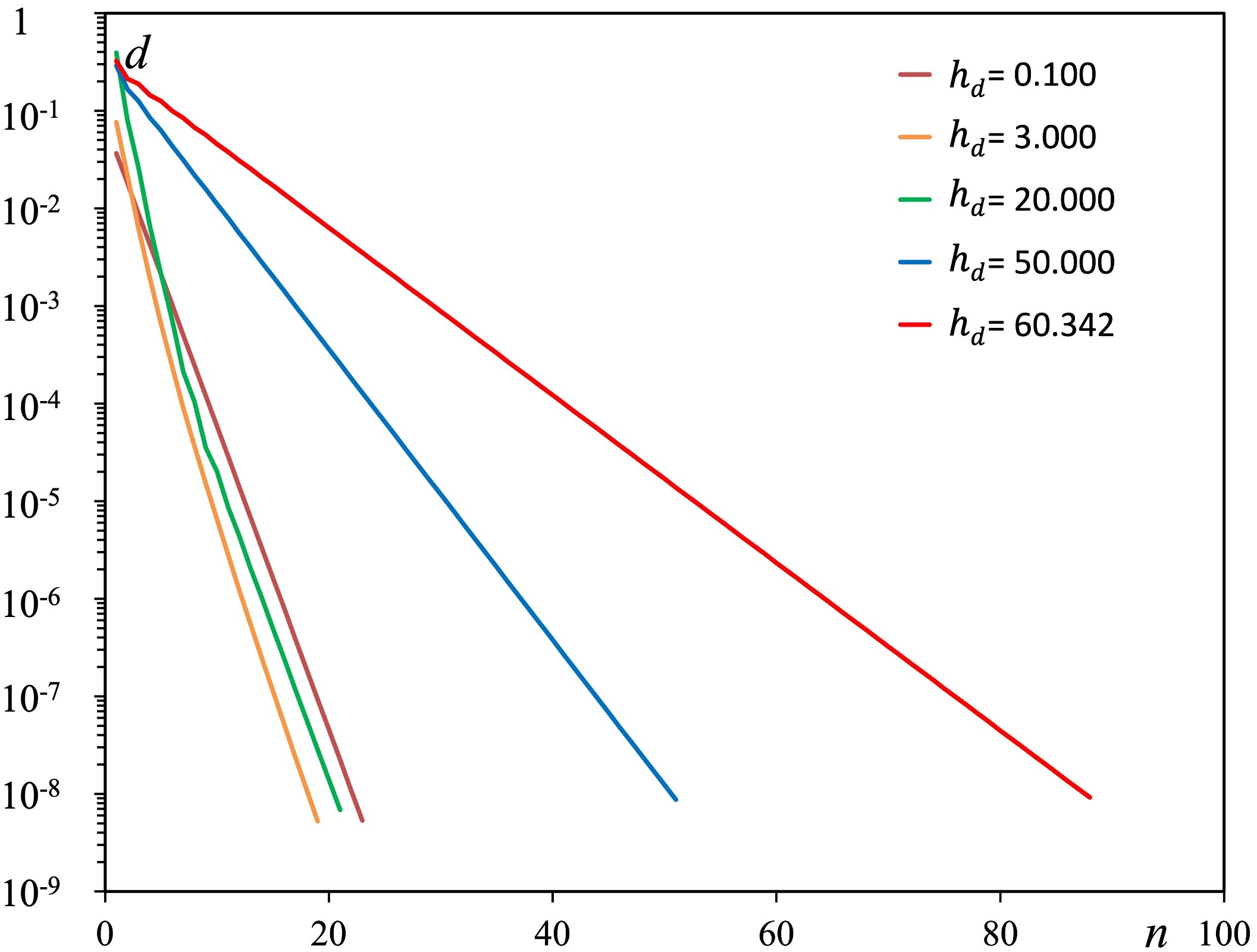
Figure 3: The deviation parameter $d$ as a function of the number of iteration $n$ for some runs with different $h_{d}$, but with other parameters the same as in the run for Figs. 1 and 2.

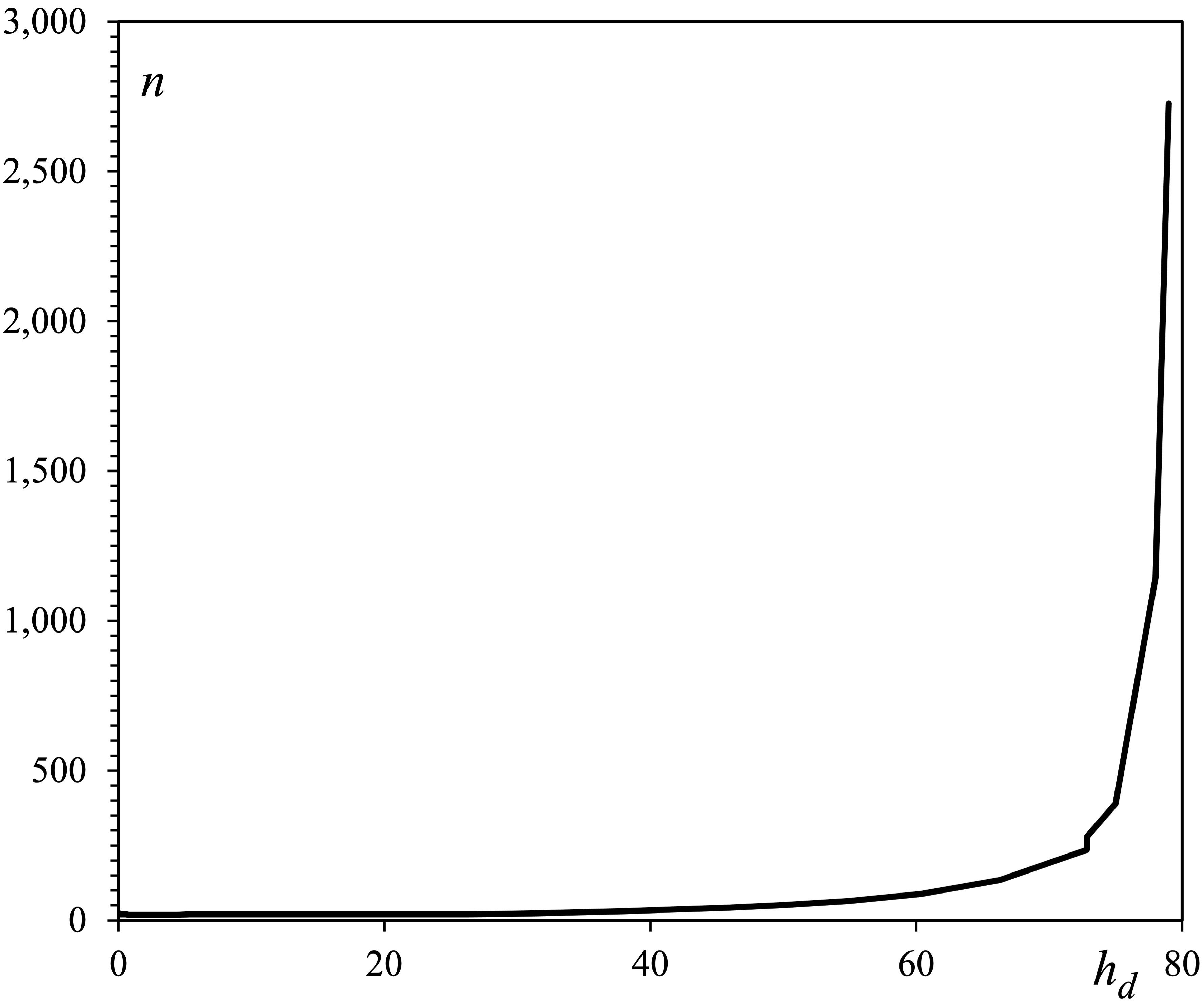
Figure 4: The number of iterations $n$ it takes for $d<10^{-8}$ as a function of $h_{d}$, using parameters the same as in Fig. 3.

In the following, we present a specific case showing that this iteration scheme is convergent up to a moderately large $h_{d}$ value. The parameters for this case are $B_{\infty}=1$, $\zeta_{i}=\tau_{i}=1/1836$, $\zeta_{d}=Z_{d}=-1$, $\beta_{d}^{2}=0.01$, $\tau_{d}=1$, and $k_{d}=-0.3$. This represents a proton plasma with an electron disk species, and with all species having the same background temperature. Obviously, this set of parameters can take many different values. However, just this one case is enough for our purpose to show the existence of solutions. Fig. 1 shows a color coded contour plot of the solution $\psi(\rho,z)$ for a run with these parameters and $h_{d}=79$, over a $1024^{2}$ grid with $\rho_{max}=11.547$, and $z_{max}=10$. The contour plot of $a_{\phi}(\rho,z)$ for this case is shown in Fig. 2. This run stops at the iteration when the $d$ value is just below the tolerance of $10^{-8}$. Many more runs with these parameters but with smaller $h_{d}$ were performed. Fig. 3 shows how $d$ changes with the number of iteration $n$ for some of these runs. We see in Fig. 3 that $d$ decreases exponentially with $n$ as $d\rightarrow 0$. However, the convergence becomes slower as $h_{d}$ increases. The $h_{d}=0.1$ case in Fig. 3 uses the iteration method as described above by setting $\psi_{i}=\psi_{f}$ and $a_{\phi i}=a_{\phi f}$ in the next iteration. It was found later that the convergence can get faster by setting the new $\psi_{i}$ and $a_{\phi i}$ as $(\psi_{i}+\psi_{f})/2$ and $(a_{\phi i}+a_{\phi f})/2$ instead. This method was used for $h_{d}=3$, which is why $d$ for this case decreases faster than the $h_{d}=0.1$ case. Obviously, this method does not change the determination of whether the solution is converged, as long as $d\rightarrow 0$. The reason why the new method has a better convergence can be traced to the fact that each iteration has a tendency of overshooting the “true” solution so that an average between the old and new solutions can result in a trial closer to the “true” solution.

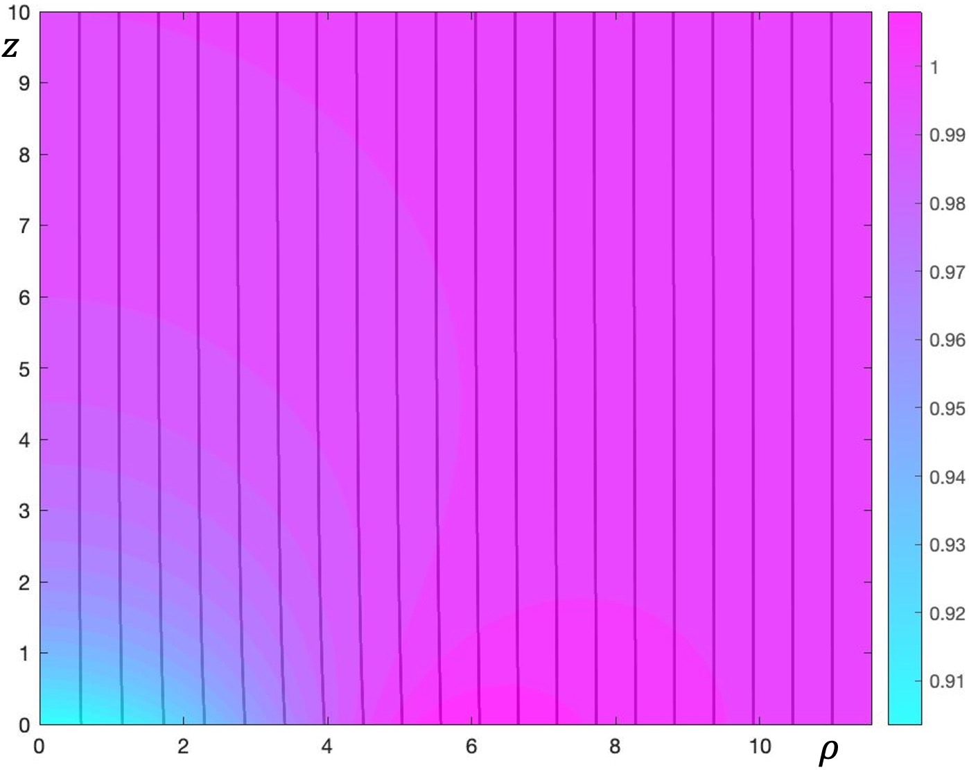
Figure 5: Color coded map for the total magnetic field strength $B$, overlaying with magnetic field lines (dark curves), from the same run for Figs. 1 and 2.

Fig. 3 does not include the $h_{d}=79$ case shown in Figs. 1 and 2 because that case converges very slowly and it takes $n=2726$ iterations for $d$ to decrease below $10^{-8}$. To show this trend, we plot the number of iterations $n$ it takes for $d<10^{-8}$ as a function of $h_{d}$ in Fig. 4. Due to the drastic increase of the number of iterations for solutions to converge as shown in Fig. 4, we have not been able to obtain converged solutions with $h_{d}>79$. Currently it is not known whether this is an absolute mathematical convergence limit, or if it can be extended by employing a different numerical method to obtain solutions. For our purpose, the existence of solutions is shown if converged solutions can be found for any finite $h_{d}$ values. The largest $h_{d}$ value of 79 in fact is corresponding to moderately large electric and magnetic field perturbations. Because we are using normalized quantities, the fact that the $\psi$ solution shown in Fig. 1 has a magnitude larger than 2 with spatial scale of the order of unity shows that the electric field is also of the order of unity, in the normalized unit. For $a_{\phi}$, the total magnetic field is the curl of it plus the background uniform magnetic field with a strength $B_{\infty}=1$. Fig. 5 shows the color coded map for the total magnetic field strength $B$, overlaying with magnetic field lines (dark curves). We see that $B$ has a decrease of about 10 % of $B_{\infty}$ around the origin, the center of the structure. Correspondingly, magnetic field lines have slight bends around the same region, although overall it looks very similar to a uniform magnetic field. The magnetic structure of such a BGK mode is diamagnetic, independent of the charge of the disk species, different from the sign of $\psi$. We confirm this with some other runs using ions as the disk species (not shown in this paper).

Finally, we remark that numerical solutions presented above have been verified in two other ways. Firstly, we have run some cases with selected $h_{d}$ values, including the $h_{d}=79$ case, on a $2048^{2}$ grid with both $\rho_{max}$ and $z_{max}$ increased by a factor of 1.5. Effectively the linear resolution for the new runs is also a factor of 1.5 higher than the old runs. It is confirm that both the new and the old run with the same $h_{d}$ have essentially the same $\psi$ and $a_{\phi}$ over the old domain, and with these fields extend to decreasingly small values in the new domain outside the old domain. Using the higher resolution and larger domain also does not change the apparent convergence limit of $h_{d}=79$. We therefore confirm that the size of the domain and the resolution used in the old runs are adequate enough to produce accurate solutions. Secondly, we substitute the final converged $\psi$ and $a_{\phi}$ solutions for cases with selected $h_{d}$ values, again including the $h_{d}=79$ case, into the set of Eqs. (10) to (13), with derivatives evaluated using second order finite differencing. We confirm that the sum of all terms for each of these equations is a small fraction of the sum of the absolute value of these terms. This provides a test of the solutions independent of the use of Hankel transforms, although we are not solving solutions using a separate numerical scheme based on a fully finite difference method.

Discussion.— In this paper, we have presented a new “Galactic Disk”-model for constructing 3D BGK mode solutions within a finite magnetic field. The main ingredient of this model that enables the existence of solutions is a rotating thin disk species, inspired by the existence of thin disk galaxies, with the recognition of the similarities between galactic dynamics and the physics of a kinetic plasma. Now that the existence of similar disk structures in a plasma is shown theoretically, it is of fundamental interest to find out whether such structures can exist in nature, or be constructed in a laboratory experiment. This is important not only to small-scale kinetic physics of plasmas, but also to the large-scale galactic dynamics. If experimental studies of disk structures in a plasma are possible, it can in turn provide insights to the dynamics of disk galaxies. There are still fundamental unsolved problems, such as the formation of spiral arm structures, partially due to the enormous time scale in galactic dynamics, making it difficult to observe how galaxies evolve in time. Studies of the dynamics of plasmas obviously do not suffer from the same problem.

This time-steady equilibrium of the disk species is enabled by a non-classical integral of motion, and maintained by a reflection symmetry. Therefore, this new model can potentially be a first step in trying to construct 3D solutions using other non-classical integrals of motion, which might allow more regular forms of solutions than the discontinuous delta-function form in the current model.

We have shown the existence of solutions for this model by presenting numerical solutions for one example with an electron disk species. The numerical method in solving these solutions is chosen because of simplicity rather than efficiency. Solutions are checked with an increase of the linear resolution and the domain size, as well as a direct substitution into equations using finite difference for derivatives. Therefore, the existence of solutions have been carefully verified, with solutions converged up to a case with moderately strong electric and magnetic field perturbations. We have not attempted to develop the numerical method further to solve for solutions more efficiently, or to extend the convergence limit of the iteration scheme. However, this should be an interesting direction for future research, to see whether solutions exist for even larger $h_{d}$ such that the magnetic field reverses direction at the center. The magnetic configuration for a self-consistent localized electron-scale equilibrium with such a magnetic field reversal would be like a spheromak.

The physical mechanism of this 3D BGK mode for a finite magnetic field is very different from the 3D BGK mode for a zero magnetic field [9], or the 3D BGK mode for an infinite magnetic field [5, 6, 7]. It is quite unlikely that our solutions can tend to these solutions in the zero or infinite field strength limits. Therefore, this shows that there can be multiple physical mechanisms for the existence of different forms of 3D BGK modes that do not tend to each other continuously. The physical mechanism is more similar to the “magnetic hole” type 2D BGK mode solutions [10, 2], except now the added electron vortex is only on a single plane while it is invariant along the whole $z$ direction for the 2D case.

Just as in many other theories of time-steady equilibrium, the existence of solutions in this model does not answer important questions regarding how such structures can form, and whether they are dynamically stable. Because these questions involve the time evolution of kinetic plasmas, they most likely can only be answered definitely by direct numerical simulations. While some preliminary studies of the stability problem for the 2D BGK modes have been conducted [15], a more comprehensive study in this direction is still on-going, since a large amount of computing is involved. The stability study for this “Galactic Disk”-model is certainly an interesting extension of this effort. Even if these disk structures turn out to be unstable, they can still be important transient phenomena, if there exists processes that can produce similar structures dynamically. Moreover, it can still be very interesting to find out what a 3D BGK mode would relax to, after an instability takes its course.

Data availability statement: Computing codes and data producing results for this paper are available at https://github.com/chungsangng/gd.