Prediction Intervals in the Beta Autoregressive Moving Average Model

B. G. Palm Programa de Pós-graduação em Engenharia de Produção, Universidade Federal de Santa Maria, RS, Brazil, E-mail: brunagpalm@gmail.com F. M. Bayer Departamento de Estatística and LACESM, Universidade Federal de Santa Maria, RS, Brazil, E-mail: bayer@ufsm.br R. J. Cintra Signal Processing Group, Departamento de Estatística, UFPE, Brazil, E-mail: rjdsc@de.ufpe.br

{onecolabstract}

In this paper, we propose five prediction intervals for the beta autoregressive moving average model. This model is suitable for modeling and forecasting variables that assume values in the interval $(0,1)$ . Two of the proposed prediction intervals are based on approximations considering the normal distribution and the quantile function of the beta distribution. We also consider bootstrap-based prediction intervals, namely: (i) bootstrap prediction errors (BPE) interval; (ii) bias-corrected and acceleration (BCa) prediction interval; and (iii) percentile prediction interval based on the quantiles of the bootstrap-predicted values for two different bootstrapping schemes. The proposed prediction intervals were evaluated according to Monte Carlo simulations. The BCa prediction interval offered the best performance among the evaluated intervals, showing lower coverage rate distortion and small average length. We applied our methodology for predicting the water level of the Cantareira water supply system in São Paulo, Brazil.

Keywords
${\beta}$ ARMA model, prediction intervals, bootstrap, time series, forecast

1 Introduction

Prediction of future values is a relevant problem in the statistical analysis of time series and it is a subject of interest in different areas of research (Homburg et al., 2020; Trucíos and Hotta, 2016; Hyndman and Athanasopoulos, 2018; Vidoni, 2009). Forecasting is often based on point estimate derived from past values of the time series under consideration (Cheung et al., 1998). However, predictions can also be presented in interval form (Pascual et al., 2005) by means of prediction intervals. Such intervals can be used as a reference for comparing different forecasting methods, facilitating the choice of the most suitable approach and the exploration of different forecasting scenarios (Chatfield, 1993; Abberger, 2006), and are widely explored in the literature. For instance, prediction intervals for count time series are discussed in Homburg et al. (2020). Prediction intervals based on a deep residual network and residual-based bootstrap methods for hydrological data are derived in Yan et al. (2021) and Beyaztas et al. (2018), respectively. In Trucíos and Hotta (2016), prediction intervals for univariate volatility models with leverage effect are introduced. Prediction intervals for long memory data are presented in Rupasinghe et al. (2014) and Rupasinghe and Samaranayake (2012).

Usually, the construction of the prediction intervals is based on: (i) the assumption that the errors of the model are normally distributed (Thombs and Schucany, 1990; Pascual et al., 2004; Clements and Kim, 2007; Li, 2011; Trucíos and Hotta, 2016) and (ii) the knowledge of the model parameters (Pascual et al., 2004; Trucíos and Hotta, 2016). However, if such conditions do not hold, then the nominal coverage of the prediction intervals can be unsatisfactory (Thombs and Schucany, 1990) and prediction intervals can be derived based on the bootstrap method, with unknown parameters and without assuming any specific distribution (Efron, 1979; Masarotto, 1990; Davison and Hinkley, 1997). This method has been widely-employed in time series modeling and it is capable of providing accurate prediction intervals and inferential improvements, as exemplified in bias correction of estimators (Palm and Bayer, 2018; Kilian, 1998), construction of confidence intervals for model parameters (Spierdijk, 2016), calculation of Fourier coefficients for the autocovariance function (Dehay et al., 2018), model selection criteria (Bayer and Cribari-Neto, 2015; Cavanaugh and Shumway, 1997), prediction intervals (Staszewska-Bystrova and Winker, 2016), and hypothesis testing (Morley and Sinclair, 2009).

A well-known and popular time series framework for modeling and forecasting is the autoregressive moving average (ARMA) model (Box et al., 2008; Oppenheim and Schafer, 2009). However, if the data under analysis do not satisfy normality, the ARMA model may not be suitable (Box et al., 2008). For instance, normal-based forecasting of data that are restricted to the interval $(0,1)$ , such as rates and proportions, can result in values outside the specific limits (Cribari-Neto and Zeileis, 2010; Ferrari and Pinheiro, 2011). This is due to the fact that the normal distribution support is the whole real line and not just the standard unit interval $(0,1)$ . Another approach for modeling of double-bounded data is the transformation of the variable of interest, $y$ . However, the results from such transformation should be interpreted in terms of the mean of the transformed variable and not of the mean of $y$ (Cribari-Neto and Zeileis, 2010). That could be in disagreement with Jensen inequality, because the conditional mean of the transformed variable may differ from the transformation of the conditional mean of the variable (Grillenzoni, 1998; White, 1984).

In this context, the beta autoregressive moving average model ( ${\beta}$ ARMA) (Rocha and Cribari-Neto, 2009) offers a suitable way to model continuous data from the interval $(0,1)$ . This particular model assumes that the variable of interest is beta-distributed. Because the support of the beta distribution is $(0,1)$ , the ${\beta}$ ARMA model forecast data is naturally suitable for continuous data in the interval $(0,1)$ , providing forecasts that are more consistent with this type of actual data. The ${\beta}$ ARMA model has been extended and explored in the literature. In Pumi et al. (2021), a dynamic model for double-bounded time series with chaotic-driven conditional averages based on the beta distribution is proposed and discussed. An study of forecasting Brazilian mortality rates due to occupational accidents using the ${\beta}$ ARMA model is presented in Melchior et al. (2020). The ${\beta}$ ARMA models for long-range dependence and sazonal series are derived in Pumi et al. (2019) and Bayer et al. (2018), respectively. Finally, bootstrap-based inferential improvements and goodness-of-fit test for hydrological time series modeling based on the ${\beta}$ ARMA model are discussed in Palm and Bayer (2018) and Scher et al. (2020), respectively.

In Rocha and Cribari-Neto (2009), it is derived an approach for point estimation, large data record results, and point forecast for the ${\beta}$ ARMA model. Nevertheless, to the best of our knowledge, the problem of deriving prediction intervals for the ${\beta}$ ARMA model has not been addressed in literature. Thus, we aim at filling this gap with a first treatment on the subject. Our goal in this paper is to present a methodology for deriving prediction intervals for the ${\beta}$ ARMA model.

One of the proposed methods is based on the beta-distribution quantiles. Another proposed interval is based on the method used in the ARMA class of models, considering the normal distribution and the variance of the prediction error (Box et al., 2008). Both intervals are considered without bootstrapping. The approach proposed in Espinheira et al. (2014) for the construction of the bias-corrected and acceleration (BCa) prediction interval for the beta regression model is adapted to the ${\beta}$ ARMA model. Another employed method is a modification of the method proposed in Masarotto (1990) for standard autoregressive models. We also considered an interval based on the quantiles of the predictions yielded from the residual and block bootstrapping schemes. The methods proposed in Box et al. (2008), Masarotto (1990), and Espinheira et al. (2014), may suffer drawbacks, such as unguaranteed assumptions of (i) knowledge of parameters (Box et al., 2008); (ii) normality when data may not be normal (Masarotto, 1990); and (iii) independence for time series data (Espinheira et al., 2014).

The paper is organized as follows. Section 2 discusses ${\beta}$ ARMA model, presenting point forecasting and residual analysis. In Section 3, the proposed prediction intervals and different types of bootstrap resampling schemes are showed. Section 4 describes Monte Carlo simulation for the proposed methods and numerical results are examined. To further evaluate the proposed method, an application to real-world measured data is detailed and discussed in Section 5. Finally, Section 6 concludes the work.

2 The Beta Autoregressive Moving Average Model

The ${\beta}$ ARMA model was proposed in Rocha and Cribari-Neto (2009) and can be described as follows. Let $\{y_{t}\}_{t\in\mathds{Z}}$ be a stochastic process for which $y_{t}\in(0,1)$ with probability 1, for all $t\in\mathds{Z}$ and let $\mathcal{F}_{t}=\sigma\{y_{t},y_{t-1},\dots\}$ denote the sigma-field generated by past observations up to time $t$ . Assume that, conditionally on the information set $\mathcal{F}_{t-1}$ , each $y_{t}$ is distributed according to $\operatorname{Beta}(\mu_{t},\phi)$ distribution, where $\mu_{t}\in(0,1)$ is the conditional mean and $\phi>0$ is the precision parameter. This parametrization of the beta distribution is commonly employed in the context of time series and regression models, where the goal is to model the mean of the response variable (Ferrari and Cribari-Neto, 2004; Rocha and Cribari-Neto, 2009). The conditional density of $y_{t}$ , given $\mathcal{F}_{t-1}$ , is (Rocha and Cribari-Neto, 2009):

\displaystyle\begin{split}f(y_{t}\mid\mathcal{F}_{t-1})=\frac{\Gamma(\phi)}{\Gamma(\mu_{t}\phi)\Gamma((1-\mu_{t})\phi)}y_{t}^{\mu_{t}\phi-1}(1-y_{t})^{(1-\mu_{t})\phi-1},\qquad 0<y_{t}<1,\quad t>0.\end{split}

(1)

The conditional mean and conditional variance of $y_{t}$ are given, respectively, by:

	$\displaystyle\operatorname{E}(y_{t}\mid\mathcal{F}_{t-1})$	$\displaystyle=\mu_{t},$
	$\displaystyle\operatorname{Var}(y_{t}\mid\mathcal{F}_{t-1})$	$\displaystyle=\frac{V(\mu_{t})}{1+\phi},$

where $V(\mu_{t})=\mu_{t}(1-\mu_{t})$ . For a fixed value of $\mu_{t}$ , the variance of $y_{t}$ decreases as $\phi$ increases (Rocha and Cribari-Neto, 2009).

The ${\beta}$ ARMA $(p,q)$ model is defined by the following structure:

g(\mu_{t})=\eta_{t}=\beta+\sum_{i=1}^{p}\varphi_{i}g(y_{t-i})+\sum_{j=1}^{q}\theta_{j}r_{t-j},

(2)

where $g:(0,1)\rightarrow\mathbb{R}$ relates $\mu_{t}$ to the linear predictor $\eta_{t}$ (Benjamin et al., 2003), being a strictly monotone, twice continuously-differentiable link function as in the beta regression model (Ferrari and Cribari-Neto, 2004); $\beta\in\mathbb{R}$ is a constant; $\varphi=(\varphi_{1},\varphi_{2},\ldots,\varphi_{p})^{\top}$ and $\theta=(\theta_{1},\theta_{2},\ldots,\theta_{q})^{\top}$ are the autoregressive and moving average parameters, respectively; and $p$ and $q$ are the orders of the model (Rocha and Cribari-Neto, 2009). The ${\beta}$ ARMA model, proposed in Rocha and Cribari-Neto (2009), also includes a term that accommodates covariates, as discussed in Benjamin et al. (2003), for a class of generalized ARMA models.

As suggested in Rocha and Cribari-Neto (2009) and Benjamin et al. (2003), the moving average term of a generalized ARMA model can be defined in several ways, such as the error on the predictor scale, $r_{t}=g(y_{t})-g(\mu_{t})$ , or on the original scale, $r_{t}=y_{t}-\mu_{t}$ . In this paper, we adopt the error on the predictor scale; thus, the model input $r_{t}$ and the model output are on the scale of $g(y_{t})$ . Therefore, the transfer function of the system, which transforms $r_{t}$ into $y_{t}$ , is given by a dynamic linear relationship that can lead to a controllable system (Box et al., 2008). The conditional variance of the error term is furnished by (Rocha and Cribari-Neto, 2009):

\displaystyle\operatorname{Var}\Big{(}g(y_{t})-g(\mu_{t})\mid\mathcal{F}_{t-1}\Big{)}=\sigma_{t}^{2}\approx\left[g^{\prime}(\mu_{t})\right]^{2}\frac{V(\mu_{t})}{1+\phi}.

(3)

The usual choices for the link function $g(\cdot)$ include the logit, probit, and complementary log-log functions (Koenker and Yoon, 2009). The parameters of the ${\beta}$ ARMA model can be estimated by maximizing the logarithm of the conditional likelihood function. More details on point estimation and large data record results for the ${\beta}$ ARMA model, conditional score function, and conditional Fisher information matrix are available in Rocha and Cribari-Neto (2009) and Rocha and Cribari-Neto (2017).

2.1 Forecasting

Let $y_{1},y_{2},\ldots,y_{n}$ be a sample from the $\beta$ ARMA model, where the conditional maximum likelihood estimation (CMLE) can be employed to obtain estimates $\widehat{\mu}_{t}$ of the conditional mean $\mu_{t}$ and $n$ is the sample size. The estimates $\widehat{\gamma}=(\widehat{\beta},\widehat{\varphi}^{\top},\widehat{\theta}^{\top},\widehat{\phi})^{\top}$ , for $\gamma=(\beta,\varphi^{\top},\theta^{\top},\phi)^{\top}$ , can be applied in Eq. (2), providing $\widehat{\mu}_{t}$ and the predicted values, $\widehat{y}_{n}(h)$ , $h$ steps forward:

\displaystyle\widehat{y}_{n}(h)=g^{-1}\left(\widehat{\beta}+\sum\limits_{i=1}^{p}\widehat{\varphi}_{i}g^{\star}(y_{n+h-i})+\sum\limits_{j=1}^{q}\widehat{\theta}_{j}r^{\star}_{n+h-j}\right),

where

\displaystyle g^{\star}(y_{n+h-i})

\displaystyle=\begin{cases}g(\widehat{y}_{n}(h-i)),&\text{if $i<h$},\\ g(y_{n+h-i}),&\text{if $i\geq h$},\end{cases}

and

\displaystyle r^{\star}_{n+h-j}

\displaystyle=\begin{cases}0,&\text{if $j<h$},\\ g(y_{n+h-j})-g(\widehat{\mu}_{n+h-j}),&\text{if $j\geq h$}.\end{cases}

The diagnostic analysis of the fitted model is based on the assessment of the behavior of residuals. The residuals are functions of the observed and predicted values one step ahead (Kedem and Fokianos, 2005). In particular, the ordinary residuals are given by (Kedem and Fokianos, 2005):

\displaystyle\mathcal{R}_{1}(y_{t},\widehat{\mu}_{t})=g(y_{t})-g(\widehat{\mu}_{t}).

As an alternative to ordinary residuals, we consider the standardized residuals (Kedem and Fokianos, 2005). For ${\beta}$ ARMA models, the standardized residuals in the predictor scale can be defined by:

\displaystyle\mathcal{R}_{2}(y_{t},\widehat{\mu}_{t})

\displaystyle=\frac{g(y_{t})-g(\widehat{\mu}_{t})}{\sqrt{[g^{\prime}(\widehat{\mu}_{t})]^{2}V(\widehat{\mu}_{t})/(1+\widehat{\phi})}}.

The radical term is an approximate estimate of the standard deviation furnished by the truncated Taylor series expansion of the variance of $r_{t}$ in Eq. (3). Another option for residual evaluation is given by (Espinheira et al., 2008):

\displaystyle\mathcal{R}_{3}(y_{t},\widehat{\mu}_{t})

\displaystyle=\frac{y_{t}^{\ast}-\widehat{\mu}_{t}^{\ast}}{\sqrt{\widehat{\nu}_{t}}},

where $\widehat{\nu}_{t}=\psi^{\prime}(\widehat{\mu}_{t}\widehat{\phi})+\psi^{\prime}(\left(1-\widehat{\mu}_{t}\right)\widehat{\phi})$ , $y_{t}^{\ast}=\log\{y_{t}/\left(1-y_{t}\right)\}$ , $\widehat{\mu}_{t}^{\ast}=\psi(\widehat{\mu}_{t}\widehat{\phi})-\psi((1-\widehat{\mu}_{t})\widehat{\phi})$ , $\psi(\cdot)$ and $\psi^{\prime}(\cdot)$ are the digamma and trigamma functions, respectively (Abramowitz and Stegun, 1964).

Zero mean and constant variance of the standardized residuals indicate a good model fit (Kedem and Fokianos, 2005). The absence of autocorrelation, partial autocorrelation, and conditional heteroscedasticity in the series of residuals are expected (Box et al., 2008). Such conditions can be verified by means of the residual correlogram or Box-Pierce (Box and Pierce, 1970), Ljung-Box (Ljung and Box, 1978), and Lagrange multiplier tests (Engle, 1982).

3 Prediction Intervals

Although, the estimate of the mean square error of a predicted value serves as an indicator of the forecast error performance, prediction intervals can offer probabilistic interpretations (Guttman, 1970; Stine, 1982). Indeed, a prediction interval is defined by the upper and lower limits associated with a prescribed probability (Chatfield, 1993) for each future value $y_{n+h}$ , $h=1,2,\ldots,H$ , where $H$ is the desirable forecast horizon.

In general, the intervals have the following format:

[LL_{h};UL_{h}],

where $LL_{h}$ and $UL_{h}$ are the lower and upper prediction limits, respectively, for $y_{n+h}$ . When the errors are not normally distributed and the parameters are unknown, the coverage rate assumes values that are lower than the nominal coverage (Thombs and Schucany, 1990; Masarotto, 1990). The coverage of the intervals is expected to be close to the nominal level, $1-\alpha$ , where $\alpha$ is the significance level. To circumvent such restrictive assumptions, bootstrap methods (Efron and Tibshirani, 1993; Davison and Hinkley, 1997) have been considered for the construction of prediction intervals, furnishing less distorted results.

The prediction intervals proposed for the ${\beta}$ ARMA model are presented in the following sections. First we introduce two prediction intervals without bootstrapping based (i) on the Box & Jenkins approach and (ii) on the quantile function of the beta distribution, which are described in Sections 3.1 and 3.2, respectively. Second we propose three bootstrap-based prediction intervals in Sections 3.3, 3.4, and 3.5. The methods are respectively based on: (i) the bootstrap prediction error; (ii) the BCa prediction interval of the beta regression model; and (iii) the quantiles of the bootstrap predicted values from two different resampling schemes.

3.1 Approximate Intervals Based on Normal Distribution (BJ)

Considering known parameters and normal moving averages errors, we introduce a variation of the Box & Jenkins (BJ) prediction interval for the ARMA model (Box et al., 2008). The BJ prediction interval for the ${\beta}$ ARMA model is proposed as follows:

	$\displaystyle LL_{h}$	$\displaystyle=g^{-1}\left\{g(\widehat{y}_{n}(h))+z_{\alpha/2}\sqrt{\widehat{V}_{n}(h)}\right\},$
	$\displaystyle UL_{h}$	$\displaystyle=g^{-1}\left\{g(\widehat{y}_{n}(h))+z_{1-\alpha/2}\sqrt{\widehat{V}_{n}(h)}\right\},$

where $z_{\alpha/2}$ and $z_{1-\alpha/2}$ are the quantiles $\alpha/2$ and $1-\alpha/2$ of the standard normal distribution, respectively. The variance of the prediction error for $h$ steps forward $V_{n}(h)$ and its estimate $\widehat{V}_{n}(h)$ is defined in Box et al. (2008) as $V_{n}(h)=(1+\Psi_{1}^{2}+\Psi_{2}^{2}+\cdots+\Psi_{H-1}^{2})\sigma^{2}_{n+h},$ where $\Psi_{j}=\varphi_{1}\Psi_{j-1}+\cdots+\varphi_{p+d}\Psi_{j-p-d}-\theta_{j}$ with $\Psi_{0}=1$ , $\Psi_{m}=0$ for $m<0$ , and $\widehat{V_{n}(h)}=(1+\widehat{\Psi}_{1}^{2}+\widehat{\Psi}_{2}^{2}+\cdots+\widehat{\Psi}_{H-1}^{2})\widehat{\sigma}^{2}_{n+h},$ where $\widehat{\Psi}_{j}=\widehat{\varphi}_{1}\widehat{\Psi}_{j-1}+\cdots+\widehat{\varphi}_{p+d}\widehat{\Psi}_{j-p-d}-\widehat{\theta_{j}}$ and $\widehat{\sigma}^{2}_{n+h}=[g^{\prime}(\widehat{y}_{n}(h))]^{2}\frac{V(\widehat{y}_{n}(h))}{1+\widehat{\phi}}$ .

3.2 Approximate Interval Based on the Beta Distribution Quantiles (Qbeta)

Another prediction interval introduced in this work is based on the beta distribution quantiles (Qbeta). We suppose that the conditional probability of the future process value $y_{n+h}$ , given the previous information up to instant $n$ , follows the beta distribution with mean $\widehat{y}_{n}(h)$ and precision $\phi_{h}$ . As the forecasting horizon increases, the variability of the prediction error also increases. To measure the loss of precision of the predicted values, we consider the following estimator of parameter $\phi_{h}$ , using Eq. (3), as:

\displaystyle{\phi}_{h}

\displaystyle\approx\frac{[g^{\prime}({\widehat{{y}}_{n}(h))}]^{2}[{\widehat{{y}}_{n}(h)}(1-\widehat{y}_{n}(h))]-{V_{n}(h)}}{{V_{n}(h)}}.

However, the value of the quantity $V_{n}(h)$ is unknown and it needs to be estimated, as shown in Box et al. (2008). An estimate for $\phi_{h}$ is directly given by:

\displaystyle\widehat{\phi}_{h}

\displaystyle=\frac{[g^{\prime}(\widehat{y}_{n}(h))]^{2}[\widehat{y}_{n}(h)(1-\widehat{y}_{n}(h))]-\widehat{V}_{n}(h)}{\widehat{V}_{n}(h)}.

As a consequence, the limits of the Qbeta prediction interval for each $h$ are furnished by:

	$\displaystyle LL_{h}$	$\displaystyle=\mathfrak{u}_{n}^{(\alpha/2)}(h),$
	$\displaystyle UL_{h}$	$\displaystyle=\mathfrak{u}_{n}^{(1-\alpha/2)}(h),$

where $\mathfrak{u}^{\alpha}_{n}(h)$ is the $\alpha$ quantile function of the $\operatorname{Beta}(\widehat{y}_{n}(h),\widehat{\phi}_{h})$ distribution.

However, the prediction intervals presented above may show lower coverage rates when compared with nominal levels, if the assumption of normality and knowledge of the parameters are not satisfied (Thombs and Schucany, 1990; Trucíos and Hotta, 2016). This issue can be addressed by means of the bootstrapping method, as it is based on the empirical distribution of the prediction errors or of the predicted values (Thombs and Schucany, 1990). In the next section, bootstrap-based prediction intervals are presented.

3.3 Bootstrap Prediction Errors Interval (BPE)

In Masarotto (1990), a bootstrap interval based on the bootstrap prediction errors (BPE) is introduced. Such method aims at building the empirical distribution of prediction errors, considering the estimated parameters by the model and the sample size of the time series. By (i) adapting the BPE interval for the ${\beta}$ ARMA model and (ii) considering the predicted value $g(\widehat{y}_{n}(h))$ and the prediction residual $\mathcal{R}_{2}(\cdot,\cdot)$ , we have the following limits:

	$\displaystyle LL_{h}^{b}$	$\displaystyle=g^{-1}\left\{g(\widehat{y}_{n}(h))+\sqrt{\left[g^{\prime}(\widehat{y}_{n}(h))\right]^{2}V(\widehat{y}_{n}(h))/(1+\widehat{\phi}_{h})}\mathcal{R}_{2(\alpha/2)}(y_{n+h}^{b},\widehat{y}^{b}_{n}(h))\right\},$
	$\displaystyle UL_{h}^{b}$	$\displaystyle=g^{-1}\left\{g(\widehat{y}_{n}(h))+\sqrt{\left[g^{\prime}(\widehat{y}_{n}(h))\right]^{2}V(\widehat{y}_{n}(h))/(1+\widehat{\phi}_{h})}\mathcal{R}_{2(1-\alpha/2)}(y_{n+h}^{b},\widehat{y}^{b}_{n}(h))\right\},$

where $\mathcal{R}_{2(\alpha/2)}(y_{n+h}^{b},\widehat{y}^{b}_{n}(h))$ and $\mathcal{R}_{2(1-\alpha/2)}(y_{n+h}^{b},\widehat{y}^{b}_{n}(h))$ are the $\alpha/2$ and $1-\alpha/2$ quantiles of the standardized residuals $\mathcal{R}_{2}(y_{n+h}^{b},\widehat{y}^{b}_{n}(h))$ , respectively, for $b=1,2,\ldots,B$ , and the quantity $B$ is the number of bootstrap replications. The bootstrap sample $y_{t}^{b}$ is an occurrence of the beta distribution with mean $\widehat{\mu}_{t}$ and precision $\widehat{\phi}$ . Each instantiation $y_{n+h}^{b}$ stems from the $\operatorname{Beta}(\widehat{y}_{n}^{b}(h),\widehat{\phi}_{h})$ distribution, where $\widehat{y}^{b}_{n}(h)$ is defined by Eq. (4).

3.4 Bias-corrected and Accelerated Bootstrap Prediction Interval

The BCa interval (Efron and Tibshirani, 1993) is based on the percentiles of the bootstrap distribution of $g(y_{n}(h))$ . The percentiles depend on $a$ and $z_{0}$ , where $a$ is the skewness correction (acceleration) and $z_{0}$ is the bias correction of $g(y_{n}(h))$ (Davison and Hinkley, 1997). Based on the distribution of the residuals of the bootstrap estimates $\mathcal{R}_{3}(y_{n+h}^{b},\widehat{y}^{b}_{n}(h))$ , the following estimate for $z_{0}$ was introduced in Espinheira et al. (2014):

\displaystyle\widehat{z}_{0}=\Phi^{-1}\left\{\frac{\#\!\left[\mathcal{R}_{3}(y_{n+h}^{b},\widehat{y}^{b}_{n}(h))<\mathcal{R}_{m})\right]}{B}\right\},

where $\Phi^{-1}(\cdot)$ is the inverse of the cumulative standard normal distribution function (Efron and Tibshirani, 1993), $\mathcal{R}_{m}$ is the median of the residuals $\mathcal{R}_{3}(y[n],\widehat{\mu}[n])$ , and $\#(\cdot)$ returns the number of times that its argument holds true. In Espinheira et al. (2014), the following estimate for $a$ was supplied:

\displaystyle\widehat{a}=\frac{1}{6}\frac{\widehat{\omega}_{n}(h)}{\widehat{\upsilon}^{3/2}_{n}(h)},

where $\widehat{\omega}_{n}(h)=\widehat{\phi}^{3}_{h}\{\psi^{\prime\prime}(\widehat{y}_{n}(h)\widehat{\phi}_{h})-\psi^{\prime\prime}((1-\widehat{y}_{n}(h))\widehat{\phi}_{h})\}$ , $\widehat{\upsilon}_{n}(h)=\widehat{\phi}^{2}_{h}\{\psi^{\prime}(\widehat{y}_{n}(h)\widehat{\phi}_{h})+\psi^{\prime}((1-\widehat{y}_{n}(h))\widehat{\phi}_{h})\}$ , and $\psi^{\prime\prime}(\cdot)$ is the derivative of the trigamma function.

The construction of the BCa prediction interval for the ${\beta}$ ARMA model is based on the algorithm presented in Espinheira et al. (2014) and Espinheira et al. (2017), where the prediction limits are given by:

	$\displaystyle LL_{h}^{b}$	$\displaystyle=\frac{1}{1+\exp\left\{-\widehat{y}^{\ast}_{n}(h)-\delta_{(\alpha/2)}\sqrt{\widehat{\nu}_{n}(h)}\right\}},$
	$\displaystyle UL_{h}^{b}$	$\displaystyle=\frac{1}{1+\exp\left\{-\widehat{y}^{\ast}_{n}(h)-\delta_{(1-\alpha/2)}\sqrt{\widehat{\nu}_{n}(h)}\right\}},$

where $\tilde{\alpha}=\Phi\left\{\widehat{z}_{0}+[(\widehat{z}_{0}+z_{\alpha})^{-1}-\widehat{a}]^{-1}\right\}$ , $\Phi(\cdot)$ is the cumulative distribution function of the standard normal distribution, $\tilde{\alpha}=\Phi\left\{\widehat{z}_{0}+[(\widehat{z}_{0}+z_{\alpha})^{-1}-\widehat{a}]^{-1}\right\}$ , $\delta_{(\alpha/2)}=\mathcal{R}_{3(\tilde{\alpha}/2)}(y_{n}^{\ast b}(h),\widehat{y}^{b}_{n}(h))$ , $\delta_{(1-\alpha/2)}=\mathcal{R}_{3(1-\tilde{\alpha}/2)}(y_{n}^{\ast b}(h),\widehat{y}^{b}_{n}(h))$ , The quantity $y_{n}^{\ast b}(h)$ is defined in Espinheira et al. (2017), $\widehat{y}^{\ast}_{n}(h)=\log(\widehat{y}_{n}(h)/(1-\widehat{y}_{n}(h)))$ , and $\widehat{\nu}_{n}(h)=\psi^{\prime}(\widehat{y}_{n}(h)\widehat{\phi}_{h})+\psi^{\prime}(\left(1-\widehat{y}_{n}(h)\right)\widehat{\phi}_{h})$ .

3.5 Bootstrap Percentile Interval

Another way to construct prediction intervals is by finding the percentiles of the $B$ replications in the considered experiment (Davison and Hinkley, 1997). For instance, one can consider the use of percentile intervals (Efron and Tibshirani, 1993), which are based on $B$ bootstrap resamplings of the predicted values $\widehat{y}_{n}(h)$ , furnishing:

\displaystyle[\widehat{y}_{n}^{I}(h);\widehat{y}_{n}^{S}(h)],

where $\widehat{y}_{n}^{I}(h)$ and $\widehat{y}_{n}^{S}(h)$ are the $\alpha/2$ and $1-\alpha/2$ quantiles of of $y_{n+h}^{b}$ , $b=1,2,\ldots,B$ .

The percentile prediction intervals were constructed considering two methods of bootstrap resampling. One approach is based on block resampling (Davison and Hinkley, 1997), and the other one is the residual method with bootstrap samples computed as

\displaystyle y_{t}^{b}=g^{-1}\left(\widehat{y}_{t}^{\ast}+\mathcal{R}_{1}^{\ast}(y_{t},\widehat{\mu}_{t})\right),

where the residuals $\mathcal{R}_{1}^{\ast}(y_{t},\widehat{\mu}_{t})$ are uniformly random draws from $\mathcal{R}_{1}(y_{1},\widehat{\mu}_{1}),\mathcal{R}_{1}(y_{2},\widehat{\mu}_{2}),\ldots,\mathcal{R}_{1}(y_{n},\widehat{\mu}_{n})$ and $\widehat{y}_{t}^{\ast}=\log\{\widehat{\mu}_{t}/(1-\widehat{\mu}_{t})$ . Bootstrap forecast realizations for future values $y_{n+h}^{b}$ are given by:

\displaystyle\widehat{y}_{n}^{b}(h)=g^{-1}\left(\widehat{\beta}^{b}+\sum_{i=1}^{p}\widehat{\varphi}_{i}^{b}g^{\star}(y_{n+h-i}^{b})+\sum_{j=1}^{q}\widehat{\theta}_{j}^{b}r_{n+h-j}^{\star b}\right),

(4)

where

\displaystyle g^{\star}(y_{n+h-i}^{b})

\displaystyle=\begin{cases}g(\widehat{y}_{n}^{b}(h-i)),&\text{if $i<h$},\\ g(y_{n+h-i}^{b}),&\text{if $i\geq h$},\end{cases}

and

\displaystyle r_{n+h-j}^{\star b}

\displaystyle=\begin{cases}g(y_{n+h-j}^{b})-g(\widehat{y}_{n}^{b}(h-j)),&\text{if $j<h$},\\ g(y_{n+h-j}^{b})-g(\widehat{\mu}^{b}_{n+h-j}),&\text{if $j\geq h$}.\end{cases}

4 Prediction Intervals Comparison

The numerical evaluation of the ${\beta}$ ARMA model prediction intervals was performed considering Monte Carlo simulations. The number $R$ of Monte Carlo replications and the number of bootstrap resampling were both set equal to $1{,}000$ , as suggested in Trucíos and Hotta (2016). The adopted sample size forecast horizon, and significance level were $n=100$ , $H=10$ , and $\alpha=0.10$ , respectively. The computational implementation was developed in R language (R Development Core Team, 2017).

We generated $n+H$ data points, where the ending $H$ observations were used to assess the prediction intervals. The structure of the mean of the ${\beta}$ ARMA model was given according to Eq. (2), employing the logit link function $\operatorname{logit}(\mu_{t})=\log(\frac{\mu_{t}}{1-\mu_{t}})$ . We analyzed the following simulation scenarios:

I.

${\beta}$ ARMA $(1,1)$ : $\beta=-0.3$ , $\varphi_{1}=-0.4$ , and $\theta_{1}=0.3$ ;
II.

${\beta}$ ARMA $(1,1)$ : $\beta=0.95$ , $\varphi_{1}=0.65$ , and $\theta_{1}=-0.95$ ;
III.

$\beta$ AR $(2)$ : $\beta=-0.3$ , $\varphi_{1}=0.8$ , and $\varphi_{2}=-0.8$ ;
IV.

$\beta$ AR $(2)$ : $\beta=0.9$ , $\varphi_{1}=0.3$ , and $\varphi_{2}=0.3$ ;
V.

$\beta$ MA $(2)$ : $\beta=-0.8$ , $\theta_{1}=0.8$ , and $\theta_{2}=-0.8$ ;
VI.

$\beta$ MA $(2)$ : $\beta=1.5$ , $\theta_{1}=-0.2$ , and $\theta_{2}=0.6$ .

The above choice of parameters aims at capturing different characterizations of $\mu$ . For example, Scenarios I, III, and V adopt $\mu\approx 0.4$ (almost symmetric distribution), and Scenarios II, IV, and VI employ $\mu\approx 0.9$ (asymmetric distribution). All models adopt $\phi=120$ . We also experimented with other values of $\phi$ , $\alpha$ , and $n$ ; however the results were not significantly different and are omitted for brevity. The results for Scenarios I and II were separated as representative cases for the parameter range of the ${\beta}$ ARMA model; results for remaining scenarios are detailed in the Appendix.

To evaluate the prediction intervals, coverage rates $(\text{CR}_{h})$ for each interval at coverage level of $90\%$ were computed according to:

\displaystyle\text{CR}_{h}=\frac{\#(LL_{h}<y_{n+h}<UL_{h})}{R}.

It is desirable that $\text{CR}_{h}$ approaches the nominal coverage level $(1-\alpha)=0.90$ . Additionally, we computed the rates for the actual future value above the upper limit or below the lower limit. Thus, we have the average upper interval $(\text{CR}_{h}^{U})$ and the average lower interval $(\text{CR}_{h}^{L})$ furnished by (Trucíos and Hotta, 2016; Pascual et al., 2004):

	$\displaystyle\text{CR}_{h}^{U}$	$\displaystyle=\frac{\#(UL_{h}<y_{n+h})}{R},$
	$\displaystyle\text{CR}_{h}^{L}$	$\displaystyle=\frac{\#(LL_{h}>y_{n+h})}{R}.$

Good prediction intervals, exhibit: $\text{CR}_{h}^{U}\approx\text{CR}_{h}^{L}\approx\alpha/2$ . The average length $(\text{A}_{h})$ of the intervals was also computed, according to (Trucíos and Hotta, 2016):

\displaystyle\text{A}_{h}

\displaystyle=\frac{1}{R}\sum\limits^{R}_{i=1}(UL_{h}^{(i)}-LL_{h}^{(i)}).

The quantity $\text{A}_{h}$ is expected to be as small as possible. The measures $\text{CR}_{h}$ , $\text{CR}_{h}^{U}$ , $\text{CR}_{h}^{L}$ , and $\text{A}_{h}$ were also considered in Thombs and Schucany (1990), Pascual et al. (2004), Pascual et al. (2006), and Trucíos and Hotta (2016) for evaluation of the prediction intervals.

To obtain an overall evaluation performance of the predicted intervals, we considered the prediction interval coverage probability (PICP) as a figure of merit, which is given by (Quan et al., 2014):

\displaystyle\text{PICP}=\frac{1}{H}\sum\limits_{h=1}^{H}\text{CR}_{h}.

PICP values that are close to the nominal coverage level indicate good performance. Finally, we computed the prediction interval normalized average width (PINAW) measure, which is defined as (Quan et al., 2014):

\displaystyle\text{PINAW}=\frac{\frac{1}{H}\sum\limits_{h=1}^{H}\text{A}_{h}}{\text{max}(y_{t})-\text{min}(y_{t})}.

The quantity PINAW is sought to be as small as possible.

Table 1 displays the Monte Carlo simulation results for Scenario I. This model consists of one autoregressive term and one moving average term with $\mu\approx 0.4$ (almost symmetric distribution). The BCa prediction interval shows values of coverage rate closer to the nominal values when compared to other prediction intervals. The Qbeta, BCa, and residual percentile prediction intervals exhibit $\text{CR}_{h}^{L}$ closer to $\text{CR}_{h}^{U}$ when compared with the remaining intervals.

Table 1: Estimated coverage rates, average length, and balanced of the prediction intervals for the Scenario I

BJ Prediction Interval
$h$	$1$	$2$	$3$	$4$	$5$	$6$	$7$	$8$	$9$	$10$
$\text{CR}_{h}$	$0.897$	$0.879$	$0.882$	$0.885$	$0.863$	$0.869$	$0.878$	$0.883$	$0.863$	$0.884$
$\text{A}_{h}$	$0.150$	$0.177$	$0.193$	$0.207$	$0.215$	$0.223$	$0.228$	$0.233$	$0.236$	$0.240$
$\text{CR}_{h}^{L}$	$0.046$	$0.061$	$0.053$	$0.064$	$0.069$	$0.070$	$0.065$	$0.062$	$0.072$	$0.057$
$\text{CR}_{h}^{U}$	$0.057$	$0.060$	$0.065$	$0.051$	$0.068$	$0.061$	$0.057$	$0.055$	$0.065$	$0.059$
Qbeta Prediction Interval
$\text{CR}_{h}$	$0.890$	$0.874$	$0.874$	$0.882$	$0.860$	$0.861$	$0.867$	$0.879$	$0.855$	$0.873$
$\text{A}_{h}$	$0.147$	$0.173$	$0.189$	$0.202$	$0.211$	$0.218$	$0.223$	$0.228$	$0.231$	$0.234$
$\text{CR}_{h}^{L}$	$0.050$	$0.064$	$0.057$	$0.063$	$0.070$	$0.072$	$0.067$	$0.062$	$0.073$	$0.058$
$\text{CR}_{h}^{U}$	$0.060$	$0.062$	$0.069$	$0.055$	$0.070$	$0.067$	$0.066$	$0.059$	$0.072$	$0.069$
BPE Prediction Interval
$\text{CR}_{h}$	$0.853$	$0.806$	$0.792$	$0.760$	$0.731$	$0.746$	$0.721$	$0.740$	$0.711$	$0.700$
$\text{A}_{h}$	$0.149$	$0.170$	$0.178$	$0.190$	$0.193$	$0.200$	$0.201$	$0.207$	$0.207$	$0.211$
$\text{CR}_{h}^{L}$	$0.078$	$0.096$	$0.110$	$0.113$	$0.152$	$0.127$	$0.156$	$0.123$	$0.164$	$0.138$
$\text{CR}_{h}^{U}$	$0.069$	$0.098$	$0.098$	$0.127$	$0.117$	$0.127$	$0.123$	$0.137$	$0.125$	$0.162$
BCa Prediction Interval
$\text{CR}_{h}$	$0.904$	$0.914$	$0.913$	$0.906$	$0.898$	$0.904$	$0.918$	$0.917$	$0.899$	$0.908$
$\text{A}_{h}$	$0.172$	$0.203$	$0.223$	$0.238$	$0.248$	$0.256$	$0.262$	$0.268$	$0.272$	$0.275$
$\text{CR}_{h}^{L}$	$0.038$	$0.050$	$0.041$	$0.052$	$0.050$	$0.048$	$0.046$	$0.036$	$0.054$	$0.043$
$\text{CR}_{h}^{U}$	$0.058$	$0.036$	$0.046$	$0.042$	$0.052$	$0.048$	$0.036$	$0.047$	$0.047$	$0.049$
Block Percentile Prediction Interval
$\text{CR}_{h}$	$0.884$	$0.879$	$0.878$	$0.874$	$0.862$	$0.861$	$0.863$	$0.863$	$0.869$	$0.877$
$\text{A}_{h}$	$0.251$	$0.252$	$0.251$	$0.251$	$0.250$	$0.250$	$0.249$	$0.249$	$0.249$	$0.249$
$\text{CR}_{h}^{L}$	$0.055$	$0.062$	$0.069$	$0.071$	$0.069$	$0.074$	$0.076$	$0.063$	$0.073$	$0.055$
$\text{CR}_{h}^{U}$	$0.061$	$0.059$	$0.053$	$0.055$	$0.069$	$0.065$	$0.061$	$0.074$	$0.058$	$0.068$
Residual Percentile Prediction Interval
$\text{CR}_{h}$	$0.951$	$0.931$	$0.920$	$0.904$	$0.890$	$0.883$	$0.889$	$0.883$	$0.874$	$0.890$
$\text{A}_{h}$	$0.226$	$0.231$	$0.235$	$0.237$	$0.240$	$0.242$	$0.243$	$0.244$	$0.246$	$0.246$
$\text{CR}_{h}^{L}$	$0.020$	$0.040$	$0.035$	$0.053$	$0.053$	$0.061$	$0.060$	$0.055$	$0.066$	$0.053$
$\text{CR}_{h}^{U}$	$0.029$	$0.029$	$0.045$	$0.043$	$0.057$	$0.056$	$0.051$	$0.062$	$0.060$	$0.057$

Figure 1 features a graphical summary of the considered measures for Qbeta, residual percentile, and BCa prediction intervals. These three intervals were separated because they behave similarly and their associated coverage rates $\text{CR}_{h}$ are closer to the nominal values for both assessed scenarios. The coverage rates are shown in Figure 1(a), being close to the nominal value of $0.90$ . The BCa prediction interval presents $\text{CR}_{h}$ values closer to the nominal level in $90\%$ of the occurrences when compared to the Qbeta and residual percentile prediction intervals. Additionally, the Qbeta and residual percentile prediction intervals present the largest variations in terms of $\text{CR}_{h}$ . Figure 1(b) presents the obtained average lengths; all the considered prediction intervals present average length values close to zero. Among the evaluated prediction intervals, the Qbeta prediction interval offers smaller values of average length but shows coverage rates farther from the nominal value, $0.90$ .

Refer to caption — (a) Comparison of the $\text{CR}_{h}$

Table 2 brings the Monte Carlo simulation results for Scenario II, which possesses one autoregressive term and one moving average term for $\mu\approx 0.9$ (asymmetric distribution). The prediction intervals offer similar results, except for the BJ prediction interval. The $\text{CR}_{h}$ values for the BJ prediction interval have noticeably departed from the values of coverage level obtained from the other prediction intervals. For instance, at $h=6$ and $h=9$ , the $\text{CR}_{h}$ values for the BJ prediction interval are equal to $0.385$ and $0.384$ , respectively. A possible reason for the distortion of the BJ prediction interval is the fact that the distribution of $y$ presents a greater asymmetry, due to the fact that $\mu=0.9$ is closer to the upper limit of the unit interval. Therefore, the normality assumption becomes inappropriate. As a consequence, BJ prediction interval performs poorly when $\mu$ is close to $0$ or $1$ . For the EPB and residual percentile prediction intervals, the values of $\text{CR}_{h}^{L}$ and $\text{CR}_{h}^{U}$ are similar when compared with the remaining prediction intervals.

Table 2: Estimated coverage rates, average length, and balanced of the prediction intervals for the Scenario II

BJ Prediction Interval
$h$	$1$	$2$	$3$	$4$	$5$	$6$	$7$	$8$	$9$	$10$
$\text{CR}_{h}$	$0.395$	$0.423$	$0.438$	$0.397$	$0.447$	$0.385$	$0.430$	$0.435$	$0.384$	$0.415$
$\text{A}_{h}$	$0.026$	$0.027$	$0.026$	$0.026$	$0.026$	$0.026$	$0.026$	$0.026$	$0.026$	$0.026$
$\text{CR}_{h}^{L}$	$0.234$	$0.252$	$0.272$	$0.304$	$0.293$	$0.315$	$0.311$	$0.288$	$0.325$	$0.296$
$\text{CR}_{h}^{U}$	$0.371$	$0.325$	$0.290$	$0.299$	$0.260$	$0.300$	$0.259$	$0.277$	$0.291$	$0.289$
Qbeta Prediction Interval
$\text{CR}_{h}$	$0.924$	$0.926$	$0.936$	$0.935$	$0.932$	$0.925$	$0.935$	$0.941$	$0.934$	$0.931$
$\text{A}_{h}$	$0.082$	$0.086$	$0.088$	$0.088$	$0.088$	$0.088$	$0.088$	$0.088$	$0.088$	$0.088$
$\text{CR}_{h}^{L}$	$0.027$	$0.041$	$0.043$	$0.038$	$0.047$	$0.044$	$0.052$	$0.043$	$0.042$	$0.046$
$\text{CR}_{h}^{U}$	$0.049$	$0.033$	$0.021$	$0.027$	$0.021$	$0.031$	$0.013$	$0.016$	$0.024$	$0.023$
BPE Prediction Interval
$\text{CR}_{h}$	$0.843$	$0.847$	$0.886$	$0.864$	$0.864$	$0.861$	$0.857$	$0.882$	$0.848$	$0.862$
$\text{A}_{h}$	$0.101$	$0.078$	$0.081$	$0.075$	$0.076$	$0.074$	$0.076$	$0.074$	$0.074$	$0.074$
$\text{CR}_{h}^{L}$	$0.005$	$0.049$	$0.056$	$0.074$	$0.085$	$0.086$	$0.100$	$0.085$	$0.106$	$0.097$
$\text{CR}_{h}^{U}$	$0.152$	$0.104$	$0.058$	$0.062$	$0.051$	$0.053$	$0.043$	$0.033$	$0.046$	$0.041$
BCa Prediction Interval
$\text{CR}_{h}$	$0.897$	$0.903$	$0.895$	$0.894$	$0.900$	$0.882$	$0.899$	$0.913$	$0.897$	$0.895$
$\text{A}_{h}$	$0.078$	$0.078$	$0.080$	$0.078$	$0.080$	$0.078$	$0.079$	$0.079$	$0.078$	$0.078$
$\text{CR}_{h}^{L}$	$0.073$	$0.068$	$0.081$	$0.067$	$0.071$	$0.067$	$0.075$	$0.061$	$0.062$	$0.066$
$\text{CR}_{h}^{U}$	$0.030$	$0.029$	$0.024$	$0.039$	$0.029$	$0.051$	$0.026$	$0.026$	$0.041$	$0.039$
Block Percentile Prediction Interval
$\text{CR}_{h}$	$0.950$	$0.926$	$0.945$	$0.924$	$0.924$	$0.915$	$0.932$	$0.933$	$0.929$	$0.926$
$\text{A}_{h}$	$0.096$	$0.090$	$0.090$	$0.088$	$0.088$	$0.088$	$0.088$	$0.088$	$0.088$	$0.088$
$\text{CR}_{h}^{L}$	$0.015$	$0.035$	$0.021$	$0.029$	$0.032$	$0.029$	$0.034$	$0.032$	$0.030$	$0.029$
$\text{CR}_{h}^{U}$	$0.035$	$0.039$	$0.034$	$0.047$	$0.044$	$0.056$	$0.034$	$0.035$	$0.041$	$0.045$
Residual Percentile Prediction Interval
$\text{CR}_{h}$	$0.940$	$0.915$	$0.916$	$0.902$	$0.906$	$0.887$	$0.906$	$0.908$	$0.899$	$0.899$
$\text{A}_{h}$	$0.088$	$0.084$	$0.082$	$0.080$	$0.080$	$0.080$	$0.080$	$0.080$	$0.080$	$0.080$
$\text{CR}_{h}^{L}$	$0.029$	$0.043$	$0.050$	$0.044$	$0.054$	$0.048$	$0.060$	$0.051$	$0.048$	$0.051$
$\text{CR}_{h}^{U}$	$0.031$	$0.042$	$0.034$	$0.054$	$0.040$	$0.065$	$0.034$	$0.041$	$0.053$	$0.050$

Figure 2(a) shows that the residual percentile and BCa prediction intervals return values for coverage rates closer to the nominal values. As discussed in Scenario I, the BCa prediction interval presents $\text{CR}_{h}$ values closer to the nominal level in comparison with the other two considered prediction intervals ( $60\%$ of the observations) and the smallest variation in the $\text{CR}_{h}$ . Additionally, Figure 2(b) presents the average length results; the BCa prediction interval is linked to the lowest average length. Thus, the BCa prediction interval offers good values of $\text{CR}_{h}$ and a small average length.

Finally, Table 3 presents the measurements of PICP and PINAW. The evaluated figures of merit are in agreement with the results based on the coverage rate and average length. The BCa and residual percentile prediction intervals outperformed the remaining methods for both considered scenarios. Moreover, a combined analysis of PICP and PINAW confirms the above conclusions, i.e., PICP is close to the nominal level and PINAW presenting small values.

Table 3: Numerical results of the figures of merit PICP and PINAW used to evaluate the prediction intervals

	Figure of merit
Prediction Interval	PICP	PINAW	PICP	PINAW
	Scenario I		Scenario II
BJ	$0.8783$	$0.2102$	$0.4149$	$0.0261$
Qbeta	$0.8715$	$0.2056$	$0.9319$	$0.0872$
BPE	$0.7560$	$0.1906$	$0.8614$	$0.0783$
BCa	$0.9081$	$0.2417$	$0.8975$	$0.0786$
Block Percentile	$0.8710$	$0.2501$	$0.9304$	$0.0892$
Residual Percentile	$0.9015$	$0.2390$	$0.9078$	$0.0814$

In a general manner, the BJ prediction interval presents values of coverage rates farther from nominal values when considering asymmetric distributions ( $\mu\approx 0.9$ ). Among the non-bootstrap-based intervals, the Qbeta prediction interval presents smaller distortions when compared to the interval BJ. On the other hand, bootstrap prediction intervals show values of $\text{CR}_{h}$ closer to the coverage level values in comparison with the prediction intervals without bootstrapping. Under Scenarios III and IV, which consider only autoregressive terms, BPE prediction interval generates values of $\text{CR}_{h}$ distant from the nominal values when compared to the results from the models that consider moving average terms. In the Appendix, we provide detailed results. This way, in the ${\beta}$ ARMA model, the use of moving average terms generates more accurate results in BPE prediction interval.

The discussed methods presented variable performances depending on the selected scenario. However, BCa prediction interval in the considered models shows smaller average length, presents $\text{CR}_{h}^{L}$ close to $\text{CR}_{h}^{U}$ , and mainly with values of $\text{CR}_{h}$ constant and close to the coverage level values of the intervals. In terms of $\text{CR}_{h}^{L}$ , $\text{CR}_{h}^{U}$ , and $\text{CR}_{h}$ , the residual prediction interval shows performance similarly to the BCa prediction interval. However, when average length is considered, the BCa prediction interval maintains its good performance; whereas the residual prediction interval offers poorer results. Thus, BCa prediction interval generally presents the best performance under all the evaluated scenarios. As a consequence, we identify the BCa prediction interval as a method capable of performing well according to all discussed figures of merit.

5 Water Level Prediction

This section presents an application of the proposed prediction intervals to measured data. The employed data set corresponds to the water level of the reservoirs from the Metropolitan Area of São Paulo, Brazil (Cantareira System) (SABESP, 2015). The water level is the proportion of water available in relation to the total storage capacity of the reservoir. The data were measured in the period of January 2003 to July 2015, consisting of 151 monthly observations. The ending ten observations were separated for assessment of the considered prediction intervals.

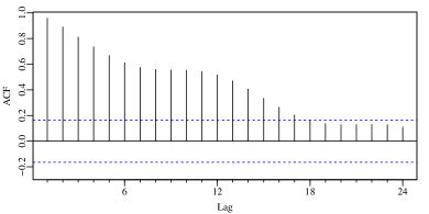
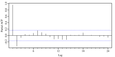
Figure 3(a) displays the considered time series with unconditional mean of $0.530$ . The kurtosis and skewness are equal to $-0.858$ and $0.054$ , respectively, indicating that the unconditional distribution of the data has shorter tails. This fact can also be verified on the data histogram in Figure 3(b). Therefore, selecting a model or a prediction interval that assumes normality would not be suitable, leading to less reliable conclusions. The maximum value of the data was $0.997$ , observed in April 2010, and the lower volume, $0.061$ , in January 2015. Figures 3(c) and 3(d) present the sampling autocorrelation function (ACF) and the sampling partial autocorrelation function (PACF), respectively.

The model selection was based on the three-stage iterative Box-Jenkins methodology (Box et al., 2008), i.e., identification (considering an exhaustive search aiming at minimizing the AIC), estimation, and diagnostic checking. Adopting a significance level of $p=0.1$ and restringing the search space to models with orders less or equal to $12$ , we successfully adjusted the employed data using the autoregressive terms $g(y_{t-1})$ , $g(y_{t-2})$ , $g(y_{t-3})$ , and $g(y_{t-4})$ , and considering the logit link function. The diagnostic analysis of the fitted model was based on the standardized residual $\mathcal{R}_{2}(y_{t},\widehat{\mu}_{t})$ . If the model is correct, then the residual is approximately normal with unit variance and around zero. Table 4 presents the fit of the selected model and the diagnostic analysis. Considering the Lagrange Multiplier, Box-Pierce, and Ljung-Box tests, the residuals of the fitted model do not exhibit conditional heteroscedasticity or autocorrelation. To perform the diagnostic tests, we followed the methodology proposed in Hyndman and Athanasopoulos (2018) to define the number of lags, which is given by: $\text{Number of lags}=\min\left(10,n/5\right)$ . As the employed data set consists of $151$ monthly observations, the number of lags is equal to $10$ .

Table 4:

{\beta}

ARMA model adjusted for the water levels of the Cantareira System.

Diagnostic analysis
	${\alpha}$	${\varphi}_{1}$	${\varphi}_{2}$	${\varphi}_{3}$	${\varphi}_{4}$	${\phi}$
Estimator	$0.0077$	$1.3838$	$-0.6626$	$0.4940$	$-0.2706$	$86.4070$
Standard Error	$0.0182$	$0.0130$	$0.0219$	$0.0307$	$0.0282$	$10.4190$
Test						$p$ -value
Lagrange Multiplier						$0.9624$
Box-Pierce						$0.1341$
Ljung-Box						$0.1153$

To assess the overall performance of the evaluated predicted intervals for water level data, we considered three figures of merit, namely: (i) coverage width-based criterion (CWC) (Quan et al., 2014); (ii) Winkler score (Score) (Quan et al., 2014; Winkler, 1972); and (iii) accumulated width deviation (AWD) (Wang et al., 2018), which are defined, respectively, as:

	CWC	$\displaystyle=\text{PINAW}+\Phi(\text{PICP})\exp\left\{-\kappa[\text{PICP}-(1-\alpha)]\right\},$
	$\displaystyle\overline{S}$	$\displaystyle=\frac{1}{H}\sum\limits_{h=1}^{H}\mid\text{S}_{h}\mid,$
	AWD	$\displaystyle=\frac{1}{H}\sum\limits_{h=1}^{H}\text{AWD}_{h},$

where $\kappa$ is a value which determines how much penalty is assigned to prediction intervals with a low coverage probability (Khosravi et al., 2010); $\Phi(\text{PICP})=0$ , for $\text{PICP}\geq 1-\alpha$ , and $\Phi(\text{PICP})=1$ , otherwise. Additionally, $\text{S}_{h}$ and $\text{AWD}_{h}$ are defined, respectively, as

\displaystyle\text{S}_{h}

\displaystyle=\begin{cases}-2\alpha A_{h}-4(LL_{h}-y_{n+h}),&\text{if $y_{n+h}<LL_{h}$},\\ -2\alpha A_{h},&\text{if $LL_{h}<y_{n+h}<UL_{h}$},\\ -2\alpha A_{h}-4(y_{n+h}-UL_{h}),&\text{if $UL_{h}>y_{n+h}$},\end{cases}

and

\displaystyle\text{AWD}_{h}

\displaystyle=\begin{cases}\frac{LL_{h}-y_{n+h}}{A_{h}},&\text{if $y_{n+h}<LL_{h}$},\\ 0,&\text{if $LL_{h}<y_{n+h}<UL_{h}$},\\ \frac{y_{n+h}-UL_{h}}{A_{h}},&\text{if $UL_{h}>y_{n+h}$}.\end{cases}

The above measures are expected to be as close to zero as possible.

Table 5 presents the measured values of PICP, PINAW, CWC, Score, and AWD of the proposed prediction intervals. We set $\kappa=2$ and $\kappa=10$ for the CWC measure aiming at evaluating its behavior variations. The Qbeta, BCa, and residual percentile prediction intervals excel in term of the considered figures of merit. Thus, the prediction intervals for measured water level show performance similar to the Monte Carlo simulations. Therefore, we recommend the use of the BCa prediction interval in order to obtain accurate prediction intervals.

Table 5: Numerical results of the prediction intervals evaluation based on PICP, PINAW, CWC, Score, and AWD figures of merit

Prediction Interval	PICP	PINAW	CWC ( $\kappa=2$ )	CWC ( $\kappa=10$ )	Score	AWD
BJ	$0.8000$	$0.2122$	$1.4336$	$2.9304$	$0.0848$	$0.0110$
Qbeta	$1.0000$	$0.3495$	$0.3495$	$0.3495$	$0.0699$	$0.0000$
BPE	$0.7000$	$0.1466$	$1.6384$	$7.5357$	$0.1498$	$0.0631$
BCa	$1.0000$	$0.8994$	$0.8994$	$0.8994$	$0.1799$	$0.0000$
Block	$0.4000$	$0.7104$	$3.4287$	$149.1236$	$0.5611$	$0.0916$
Residual	$0.9000$	$0.6566$	$0.6566$	$0.6566$	$0.1504$	$0.0004$

We also performed a sensitivity analysis based on the BCa prediction interval considering the methodology proposed in Wang et al. (2018) and Espinheira et al. (2014). For such, we constructed BCa prediction intervals considering four different number of bootstrap replications aiming at capturing the effectiveness and robustness of the prediction interval. The sensitivity analysis was evaluated in terms of PICP, PINAW, CWC, Score, and AWD figures of merit; the results are presented in Table 6. We note that the coverage rate and average length remained constant when we increased the number of bootstrap replications, i.e., PICP, PINAW, CWC, Score, and AWD show similar values regardless of the considered number of iterations.

Table 6: Numerical results of the BCa prediction interval sensitivity analysis

Number of bootstrap iterations	PICP	PINAW	CWC ( $\kappa=2$ )	Score	AWD
$500$	$1.0000$	$0.8706$	$0.8706$	$0.1741$	$0.0000$
$1000$	$1.0000$	$0.8994$	$0.8994$	$0.1799$	$0.0000$
$2000$	$1.0000$	$0.8962$	$0.8962$	$0.1792$	$0.0000$
$5000$	$1.0000$	$0.8896$	$0.8896$	$0.1779$	$0.0000$

Finally, we compared BCa prediction interval to the prediction interval furnished by the traditional ARMA model (Box et al., 2008). Figure 4 presents the last 12 observations with the last ten original data values and prediction interval BCa for $\alpha=0.10$ . For all observations, the BCa prediction interval presents prediction limits within the support of the data, while the lower limits of the ARMA model prediction interval show values smaller than zero. Thus, the results from the ARMA model lack physical meaning because the data of interest is defined over the interval $(0,1)$ . This application emphasizes the importance of a judicious model selection for the construction of reliable prediction intervals for beta-distributed time series data. In the ARMA model case, the erroneous assumption of normality led to results without clear meaning, since they were outside the interval $(0,1)$ . The proposed BCa prediction interval in $\beta$ ARMA model was identified as the most suitable interval for this type of data.

6 Conclusions

Generally, the ARMA models are used for modeling and forecasting variables over time. ARMA models may not be suitable when the variable of interest does not satisfy normality, as exemplified by variables that take values in the continuous interval $(0,1)$ , such as rates and proportions. Under such conditions, the ${\beta}$ ARMA model, which assumes the beta distribution to the variable of interest, becomes a more appropriate tool.

The present work proposed five methods for deriving prediction intervals under the ${\beta}$ ARMA model. Two of the introduced methods do not require bootstrapping and are based on the predictions intervals for ARMA model and beta quantiles distributions. The remaining three proposed methods resort to bootstrapping and stem from the BPE, BCa, and percentile intervals.

The prediction intervals with bootstrapping presented better coverage rate than the non-bootstrapping intervals. The BCa prediction interval exhibited constant values in all scenarios considered, with lower average length and coverage rates close to nominal values. Thus, the BCa prediction interval is more reliable, regardless of the discussed scenarios.

The proposed intervals methods were applied to measured data from reservoir water level in the Metropolitan Area of São Paulo. BCa prediction interval was considered and compared to the traditional ARMA models. The limits of the ARMA model prediction interval presented negative values in clear conflict with the support of the data of interest. Such mismatch highlights the necessity of choosing an appropriate prediction interval. Moreover, the proposed BCa prediction interval showed values within the correct interval $(0,1)$ . As a conclusion, we recommend the use of the BCa prediction interval for constructing of accurate prediction intervals for data restricted to the interval $(0,1)$ . In future studies, we aim at addressing prediction intervals for the ${\beta}$ ARMA model in the presence of long dependence (Pumi et al., 2019) and seasonality (Bayer et al., 2018), as well as, for competitive models that assume other distributions for the doubly limited response variable, such as Kumaraswamy (Bayer et al., 2017) and beta binomial (Palm et al., 2021).

Acknowledgements

We gratefully acknowledge partial financial support from Fundação de Amparo à Pesquisa do Estado do Rio Grande do Sul (FAPERGS), Conselho Nacional de Desenvolvimento Científico and Tecnológico (CNPq), and Coordenação de Aperfeiçoamento de Pessoal de Nível Superior (CAPES), Brazil.

Appendix

In this appendix, the numerical results for Scenarios III, IV, V, and VI are presented with coverage level equal to $0.90$ . Tables 7 and 8 show the numerical results of simulations for Scenarios III and V, respectively, with $\mu\approx 0.4$ and $n=100$ . Scenarios IV and VI are found in Tables 9 and 10, respectively, for $n=100$ and $\mu\approx 0.9$ .

Table 7: Estimated coverage rates, average length, and balanced of the prediction intervals for the Scenario III

BJ Prediction Interval
$h$	$1$	$2$	$3$	$4$	$5$	$6$	$7$	$8$	$9$	$10$
$\text{CR}_{h}$	$0.900$	$0.878$	$0.883$	$0.877$	$0.887$	$0.891$	$0.885$	$0.900$	$0.890$	$0.888$
$\text{A}_{h}$	$0.146$	$0.187$	$0.188$	$0.218$	$0.230$	$0.233$	$0.246$	$0.250$	$0.252$	$0.260$
$\text{CR}_{h}^{L}$	$0.054$	$0.062$	$0.054$	$0.068$	$0.053$	$0.054$	$0.056$	$0.058$	$0.048$	$0.057$
$\text{CR}_{h}^{U}$	$0.046$	$0.060$	$0.063$	$0.055$	$0.060$	$0.055$	$0.059$	$0.042$	$0.062$	$0.055$
Qbeta Prediction Interval
$\text{CR}_{h}$	$0.895$	$0.882$	$0.883$	$0.884$	$0.891$	$0.893$	$0.886$	$0.899$	$0.891$	$0.891$
$\text{A}_{h}$	$0.146$	$0.187$	$0.189$	$0.219$	$0.231$	$0.234$	$0.248$	$0.251$	$0.254$	$0.261$
$\text{CR}_{h}^{L}$	$0.054$	$0.059$	$0.053$	$0.062$	$0.047$	$0.048$	$0.055$	$0.058$	$0.043$	$0.054$
$\text{CR}_{h}^{U}$	$0.051$	$0.059$	$0.064$	$0.054$	$0.062$	$0.059$	$0.059$	$0.043$	$0.066$	$0.055$
BPE Prediction Interval
$\text{CR}_{h}$	$0.685$	$0.646$	$0.687$	$0.657$	$0.673$	$0.646$	$0.672$	$0.658$	$0.646$	$0.653$
$\text{A}_{h}$	$0.107$	$0.134$	$0.140$	$0.163$	$0.171$	$0.175$	$0.185$	$0.187$	$0.189$	$0.195$
$\text{CR}_{h}^{L}$	$0.150$	$0.177$	$0.166$	$0.160$	$0.155$	$0.186$	$0.158$	$0.168$	$0.173$	$0.177$
$\text{CR}_{h}^{U}$	$0.165$	$0.177$	$0.147$	$0.183$	$0.172$	$0.168$	$0.170$	$0.174$	$0.181$	$0.170$
BCa Prediction Interval
$\text{CR}_{h}$	$0.814$	$0.855$	$0.842$	$0.862$	$0.895$	$0.883$	$0.882$	$0.903$	$0.899$	$0.904$
$\text{A}_{h}$	$0.142$	$0.193$	$0.198$	$0.236$	$0.251$	$0.252$	$0.269$	$0.274$	$0.277$	$0.287$
$\text{CR}_{h}^{L}$	$0.088$	$0.065$	$0.078$	$0.070$	$0.048$	$0.057$	$0.051$	$0.053$	$0.048$	$0.049$
$\text{CR}_{h}^{U}$	$0.098$	$0.080$	$0.080$	$0.068$	$0.057$	$0.060$	$0.067$	$0.044$	$0.053$	$0.047$
Block Percentile Prediction Interval
$\text{CR}_{h}$	$0.891$	$0.892$	$0.873$	$0.886$	$0.904$	$0.875$	$0.879$	$0.894$	$0.886$	$0.886$
$\text{A}_{h}$	$0.261$	$0.273$	$0.270$	$0.271$	$0.272$	$0.271$	$0.271$	$0.271$	$0.271$	$0.271$
$\text{CR}_{h}^{L}$	$0.050$	$0.055$	$0.069$	$0.059$	$0.049$	$0.064$	$0.055$	$0.058$	$0.054$	$0.061$
$\text{CR}_{h}^{U}$	$0.059$	$0.053$	$0.058$	$0.055$	$0.047$	$0.061$	$0.066$	$0.048$	$0.060$	$0.053$
Residual Percentile Prediction Interval
$\text{CR}_{h}$	$0.929$	$0.917$	$0.896$	$0.882$	$0.910$	$0.884$	$0.877$	$0.898$	$0.888$	$0.880$
$\text{A}_{h}$	$0.247$	$0.251$	$0.263$	$0.269$	$0.269$	$0.272$	$0.272$	$0.273$	$0.273$	$0.273$
$\text{CR}_{h}^{L}$	$0.032$	$0.037$	$0.057$	$0.062$	$0.043$	$0.059$	$0.055$	$0.056$	$0.053$	$0.062$
$\text{CR}_{h}^{U}$	$0.039$	$0.046$	$0.047$	$0.056$	$0.047$	$0.057$	$0.068$	$0.046$	$0.059$	$0.058$

Table 8: Estimated coverage rates, average length, and balanced of the prediction intervals for the Scenario V

BJ Prediction Interval
$h$	$1$	$2$	$3$	$4$	$5$	$6$	$7$	$8$	$9$	$10$
$\text{CR}_{h}$	$0.854$	$0.880$	$0.846$	$0.845$	$0.847$	$0.841$	$0.820$	$0.875$	$0.847$	$0.832$
$\text{A}_{h}$	$0.182$	$0.183$	$0.183$	$0.183$	$0.183$	$0.183$	$0.183$	$0.183$	$0.183$	$0.183$
$\text{CR}_{h}^{L}$	$0.098$	$0.067$	$0.083$	$0.097$	$0.081$	$0.085$	$0.104$	$0.064$	$0.087$	$0.095$
$\text{CR}_{h}^{U}$	$0.048$	$0.053$	$0.071$	$0.058$	$0.072$	$0.074$	$0.076$	$0.061$	$0.066$	$0.073$
Qbeta Prediction Interval
$\text{CR}_{h}$	$0.918$	$0.919$	$0.902$	$0.907$	$0.902$	$0.898$	$0.888$	$0.918$	$0.905$	$0.887$
$\text{A}_{h}$	$0.208$	$0.211$	$0.211$	$0.211$	$0.211$	$0.211$	$0.211$	$0.211$	$0.211$	$0.211$
$\text{CR}_{h}^{L}$	$0.052$	$0.040$	$0.050$	$0.050$	$0.040$	$0.049$	$0.053$	$0.042$	$0.045$	$0.055$
$\text{CR}_{h}^{U}$	$0.030$	$0.041$	$0.048$	$0.043$	$0.058$	$0.053$	$0.059$	$0.040$	$0.050$	$0.058$
BPE Prediction Interval
$\text{CR}_{h}$	$0.828$	$0.835$	$0.840$	$0.837$	$0.836$	$0.840$	$0.820$	$0.855$	$0.851$	$0.835$
$\text{A}_{h}$	$0.191$	$0.193$	$0.195$	$0.194$	$0.194$	$0.194$	$0.194$	$0.194$	$0.194$	$0.194$
$\text{CR}_{h}^{L}$	$0.100$	$0.076$	$0.081$	$0.083$	$0.077$	$0.074$	$0.093$	$0.078$	$0.075$	$0.081$
$\text{CR}_{h}^{U}$	$0.072$	$0.089$	$0.079$	$0.080$	$0.087$	$0.086$	$0.087$	$0.067$	$0.074$	$0.084$
BCa Prediction Interval
$\text{CR}_{h}$	$0.854$	$0.884$	$0.899$	$0.910$	$0.896$	$0.900$	$0.890$	$0.909$	$0.906$	$0.888$
$\text{A}_{h}$	$0.199$	$0.203$	$0.212$	$0.212$	$0.212$	$0.212$	$0.212$	$0.212$	$0.212$	$0.212$
$\text{CR}_{h}^{L}$	$0.079$	$0.051$	$0.044$	$0.045$	$0.041$	$0.046$	$0.051$	$0.042$	$0.039$	$0.052$
$\text{CR}_{h}^{U}$	$0.067$	$0.065$	$0.057$	$0.045$	$0.063$	$0.054$	$0.059$	$0.049$	$0.055$	$0.060$
Block Percentile Prediction Interval
$\text{CR}_{h}$	$0.860$	$0.875$	$0.896$	$0.907$	$0.896$	$0.898$	$0.885$	$0.916$	$0.906$	$0.880$
$\text{A}_{h}$	$0.198$	$0.200$	$0.209$	$0.208$	$0.208$	$0.208$	$0.209$	$0.209$	$0.208$	$0.209$
$\text{CR}_{h}^{L}$	$0.078$	$0.059$	$0.053$	$0.053$	$0.042$	$0.050$	$0.060$	$0.045$	$0.045$	$0.065$
$\text{CR}_{h}^{U}$	$0.062$	$0.066$	$0.051$	$0.040$	$0.062$	$0.052$	$0.055$	$0.039$	$0.049$	$0.055$
Residual Percentile Prediction Interval
$\text{CR}_{h}$	$0.881$	$0.882$	$0.898$	$0.900$	$0.895$	$0.901$	$0.884$	$0.920$	$0.901$	$0.883$
$\text{A}_{h}$	$0.206$	$0.2084$	$0.209$	$0.209$	$0.209$	$0.210$	$0.209$	$0.209$	$0.210$	$0.210$
$\text{CR}_{h}^{L}$	$0.069$	$0.060$	$0.049$	$0.057$	$0.043$	$0.050$	$0.061$	$0.044$	$0.048$	$0.061$
$\text{CR}_{h}^{U}$	$0.050$	$0.058$	$0.053$	$0.043$	$0.062$	$0.049$	$0.055$	$0.036$	$0.051$	$0.056$

Table 9: Estimated coverage rates, average length, and balanced of the prediction intervals for the Scenario IV

BJ Prediction Interval
$h$	$1$	$2$	$3$	$4$	$5$	$6$	$7$	$8$	$9$	$10$
$\text{CR}_{h}$	$0.459$	$0.468$	$0.487$	$0.493$	$0.470$	$0.458$	$0.490$	$0.475$	$0.481$	$0.459$
$\text{A}_{h}$	$0.035$	$0.037$	$0.039$	$0.040$	$0.041$	$0.041$	$0.042$	$0.042$	$0.042$	$0.042$
$\text{CR}_{h}^{L}$	$0.250$	$0.231$	$0.224$	$0.207$	$0.210$	$0.220$	$0.190$	$0.206$	$0.207$	$0.213$
$\text{CR}_{h}^{U}$	$0.291$	$0.301$	$0.289$	$0.300$	$0.320$	$0.322$	$0.320$	$0.319$	$0.312$	$0.328$
Qbeta Prediction Interval
$\text{CR}_{h}$	$0.886$	$0.886$	$0.885$	$0.869$	$0.894$	$0.859$	$0.890$	$0.885$	$0.867$	$0.860$
$\text{A}_{h}$	$0.084$	$0.088$	$0.094$	$0.096$	$0.097$	$0.098$	$0.098$	$0.099$	$0.099$	$0.099$
$\text{CR}_{h}^{L}$	$0.069$	$0.068$	$0.060$	$0.055$	$0.050$	$0.060$	$0.037$	$0.040$	$0.053$	$0.057$
$\text{CR}_{h}^{U}$	$0.045$	$0.046$	$0.055$	$0.076$	$0.056$	$0.081$	$0.073$	$0.075$	$0.080$	$0.083$
BPE Prediction Interval
$\text{CR}_{h}$	$0.745$	$0.750$	$0.779$	$0.775$	$0.786$	$0.773$	$0.799$	$0.814$	$0.783$	$0.800$
$\text{A}_{h}$	$0.076$	$0.082$	$0.089$	$0.091$	$0.092$	$0.092$	$0.093$	$0.093$	$0.093$	$0.093$
$\text{CR}_{h}^{L}$	$0.068$	$0.062$	$0.065$	$0.063$	$0.068$	$0.088$	$0.067$	$0.069$	$0.074$	$0.080$
$\text{CR}_{h}^{U}$	$0.187$	$0.188$	$0.156$	$0.162$	$0.146$	$0.139$	$0.134$	$0.117$	$0.143$	$0.120$
BCa Prediction Interval
$\text{CR}_{h}$	$0.857$	$0.863$	$0.876$	$0.865$	$0.879$	$0.869$	$0.882$	$0.894$	$0.870$	$0.873$
$\text{A}_{h}$	$0.083$	$0.088$	$0.094$	$0.096$	$0.097$	$0.097$	$0.097$	$0.098$	$0.098$	$0.098$
$\text{CR}_{h}^{L}$	$0.091$	$0.088$	$0.083$	$0.076$	$0.072$	$0.076$	$0.062$	$0.061$	$0.067$	$0.075$
$\text{CR}_{h}^{U}$	$0.052$	$0.049$	$0.041$	$0.059$	$0.049$	$0.055$	$0.056$	$0.045$	$0.063$	$0.052$
Block Percentile Prediction Interval
$\text{CR}_{h}$	$0.906$	$0.912$	$0.905$	$0.884$	$0.909$	$0.895$	$0.908$	$0.913$	$0.894$	$0.881$
$\text{A}_{h}$	$0.105$	$0.106$	$0.106$	$0.106$	$0.107$	$0.106$	$0.106$	$0.106$	$0.106$	$0.106$
$\text{CR}_{h}^{L}$	$0.046$	$0.044$	$0.050$	$0.045$	$0.038$	$0.044$	$0.029$	$0.033$	$0.040$	$0.055$
$\text{CR}_{h}^{U}$	$0.048$	$0.044$	$0.045$	$0.071$	$0.053$	$0.061$	$0.063$	$0.054$	$0.066$	$0.064$
Residual Percentile Prediction Interval
$\text{CR}_{h}$	$0.916$	$0.894$	$0.891$	$0.873$	$0.895$	$0.873$	$0.895$	$0.901$	$0.876$	$0.872$
$\text{A}_{h}$	$0.098$	$0.099$	$0.099$	$0.099$	$0.099$	$0.099$	$0.099$	$0.099$	$0.099$	$0.099$
$\text{CR}_{h}^{L}$	$0.050$	$0.059$	$0.062$	$0.057$	$0.052$	$0.064$	$0.045$	$0.043$	$0.056$	$0.063$
$\text{CR}_{h}^{U}$	$0.034$	$0.047$	$0.047$	$0.070$	$0.053$	$0.063$	$0.060$	$0.056$	$0.068$	$0.065$

Table 10: Estimated coverage rates, average length, and balanced of the prediction intervals for the Scenario VI

BJ Prediction Interval
$h$	$1$	$2$	$3$	$4$	$5$	$6$	$7$	$8$	$9$	$10$
$\text{CR}_{h}$	$0.825$	$0.820$	$0.745$	$0.737$	$0.767$	$0.761$	$0.755$	$0.773$	$0.751$	$0.755$
$\text{A}_{h}$	$0.097$	$0.099$	$0.099$	$0.099$	$0.099$	$0.099$	$0.099$	$0.099$	$0.099$	$0.099$
$\text{CR}_{h}^{L}$	$0.060$	$0.065$	$0.105$	$0.099$	$0.090$	$0.099$	$0.091$	$0.096$	$0.095$	$0.096$
$\text{CR}_{h}^{U}$	$0.115$	$0.115$	$0.150$	$0.164$	$0.143$	$0.140$	$0.154$	$0.131$	$0.1544$	$0.149$
Qbeta Prediction Interval
$\text{CR}_{h}$	$0.955$	$0.948$	$0.904$	$0.891$	$0.907$	$0.905$	$0.906$	$0.903$	$0.905$	$0.890$
$\text{A}_{h}$	$0.138$	$0.140$	$0.140$	$0.140$	$0.140$	$0.140$	$0.140$	$0.140$	$0.140$	$0.140$
$\text{CR}_{h}^{L}$	$0.018$	$0.025$	$0.043$	$0.043$	$0.037$	$0.044$	$0.039$	$0.048$	$0.043$	$0.047$
$\text{CR}_{h}^{U}$	$0.027$	$0.027$	$0.053$	$0.066$	$0.056$	$0.051$	$0.055$	$0.049$	$0.052$	$0.063$
BPE Prediction Interval
$\text{CR}_{h}$	$0.824$	$0.828$	$0.790$	$0.784$	$0.809$	$0.809$	$0.795$	$0.801$	$0.794$	$0.798$
$\text{A}_{h}$	$0.119$	$0.121$	$0.122$	$0.123$	$0.122$	$0.122$	$0.122$	$0.122$	$0.122$	$0.122$
$\text{CR}_{h}^{L}$	$0.085$	$0.089$	$0.099$	$0.077$	$0.083$	$0.088$	$0.090$	$0.095$	$0.089$	$0.095$
$\text{CR}_{h}^{U}$	$0.091$	$0.083$	$0.111$	$0.139$	$0.108$	$0.103$	$0.115$	$0.104$	$0.117$	$0.107$
BCa Prediction Interval
$\text{CR}_{h}$	$0.883$	$0.883$	$0.901$	$0.882$	$0.907$	$0.893$	$0.898$	$0.888$	$0.898$	$0.880$
$\text{A}_{h}$	$0.124$	$0.129$	$0.137$	$0.137$	$0.137$	$0.137$	$0.137$	$0.137$	$0.137$	$0.137$
$\text{CR}_{h}^{L}$	$0.061$	$0.064$	$0.048$	$0.058$	$0.047$	$0.060$	$0.051$	$0.061$	$0.053$	$0.061$
$\text{CR}_{h}^{U}$	$0.056$	$0.053$	$0.051$	$0.060$	$0.046$	$0.047$	$0.051$	$0.051$	$0.049$	$0.059$
Block Percentile Prediction Interval
$\text{CR}_{h}$	$0.898$	$0.890$	$0.899$	$0.885$	$0.902$	$0.902$	$0.897$	$0.895$	$0.897$	$0.889$
$\text{A}_{h}$	$0.128$	$0.132$	$0.137$	$0.137$	$0.137$	$0.137$	$0.137$	$0.137$	$0.137$	$0.138$
$\text{CR}_{h}^{L}$	$0.041$	$0.051$	$0.046$	$0.046$	$0.041$	$0.046$	$0.045$	$0.050$	$0.049$	$0.053$
$\text{CR}_{h}^{U}$	$0.061$	$0.059$	$0.055$	$0.069$	$0.057$	$0.052$	$0.058$	$0.055$	$0.054$	$0.058$
Residual Percentile Prediction Interval
$\text{CR}_{h}$	$0.914$	$0.900$	$0.898$	$0.878$	$0.903$	$0.893$	$0.900$	$0.898$	$0.897$	$0.888$
$\text{A}_{h}$	$0.135$	$0.137$	$0.137$	$0.137$	$0.137$	$0.137$	$0.137$	$0.1374$	$0.137$	$0.137$
$\text{CR}_{h}^{L}$	$0.037$	$0.049$	$0.048$	$0.052$	$0.038$	$0.049$	$0.041$	$0.049$	$0.048$	$0.049$
$\text{CR}_{h}^{U}$	$0.049$	$0.051$	$0.054$	$0.070$	$0.059$	$0.058$	$0.059$	$0.053$	$0.055$	$0.063$

References

Abberger (2006) Abberger, K. (2006). Kernel smoothed prediction intervals for ARMA models. Statistical Papers, 47(1), 1–15.
Abramowitz and Stegun (1964) Abramowitz, M., Stegun, I. A. (1964). Handbook of mathematical functions: With formulas, graphs, and mathematical tables, vol 55. Courier Corporation.
Bayer and Cribari-Neto (2015) Bayer, F. M., Cribari-Neto, F. (2015). Bootstrap-based model selection criteria for beta regressions. Test, 24(4), 776–795.
Bayer et al. (2017) Bayer, F. M., Bayer, D. M., Pumi, G. (2017). Kumaraswamy autoregressive moving average models for double bounded environmental data. Journal of Hydrology, 555, 385–396.
Bayer et al. (2018) Bayer, F. M., Cintra, R. J., Cribari-Neto, F. (2018). Beta seasonal autoregressive moving average models. Journal of Statistical Computation and Simulation, 88(15), 2961–2981.
Benjamin et al. (2003) Benjamin, M. A., Rigby, R. A., Stasinopoulos, D. M. (2003). Generalized autoregressive moving average models. Journal of the American Statistical Association, 98(461), 214–223.
Beyaztas et al. (2018) Beyaztas, U., Arikan, B. B., Beyaztas, B. H., Kahya, E. (2018). Construction of prediction intervals for Palmer Drought Severity Index using bootstrap. Journal of Hydrology, 559, 461–470.
Box et al. (2008) Box, G., Jenkins, G. M., Reinsel, G. (2008). Time series analysis: Forecasting and control. Hardcover, John Wiley & Sons.
Box and Pierce (1970) Box, G. E. P., Pierce, D. A. (1970). Distribution of residual autocorrelations in autoregressive-integrated moving average time series models. Journal of the American Statistical Association, 65(332), 1509–1526.
Cavanaugh and Shumway (1997) Cavanaugh, J. E., Shumway, R. H. (1997). A bootstrap variant of AIC for state-space model selection. Statistica Sinica, 7(2), 473–496.
Chatfield (1993) Chatfield, C. (1993). Calculating interval forecasts. Journal of Business & Economic Statistics, 11(2), 121–135.
Cheung et al. (1998) Cheung, S. H., Wu, K. H., Chan, W. S. (1998). Simultaneous prediction intervals for autoregressive integrated moving average models: A comparative study. Computacional Statistics & Data Analysis, 28(3), 297–306.
Clements and Kim (2007) Clements, M. P., Kim (2007). Bootstrap prediction intervals for autoregressive time series. Computacional Statistics & Data Analysis, 51(7), 3580–3594.
Cribari-Neto and Zeileis (2010) Cribari-Neto, F., Zeileis, A. (2010). Beta regression in R. Journal of Statistical Software, 34(2).
Davison and Hinkley (1997) Davison, A. C., Hinkley, D. V. (1997). Bootstrap methods and their application. Cambridge University Press.
Dehay et al. (2018) Dehay, D., Dudek, A. E., El Badaoui, M. (2018). Bootstrap for almost cyclostationary processes with jitter effect. Digital Signal Processing, 73, 93–105.
Efron (1979) Efron, B. (1979). Bootstrap methods: another look at the jackknife. The Annals of Statistics, 7(1), 1–26.
Efron and Tibshirani (1993) Efron, B., Tibshirani, R. J. (1993). An introduction to the bootstrap. Chapman & Hall.
Engle (1982) Engle, R. F. (1982). Autoregressive conditional heteroskedasticity with estimates of the variance of UK inflation. Econometrica, 50(4), 987–1007.
Espinheira et al. (2008) Espinheira, P. L., Ferrari, S. L. P., Cribari-Neto, F. (2008). On beta regression residuals. Journal of Applied Statistics, 35(4), 407–419.
Espinheira et al. (2014) Espinheira, P. L., Ferrari, S. L., Cribari-Neto, F. (2014). Bootstrap prediction intervals in beta regressions. Computational Statistics, 29(5), 1263–1277.
Espinheira et al. (2017) Espinheira, P. L., Ferrari, S. L., Cribari-Neto, F. (2017). Erratum to: Bootstrap prediction intervals in beta regressions. Computational Statistics, 32(4), 1777–1777.
Ferrari and Cribari-Neto (2004) Ferrari, S. L. P., Cribari-Neto, F. (2004). Beta regression for modelling rates and proportions. Journal of Applied Statistics, 31(7), 799–815.
Ferrari and Pinheiro (2011) Ferrari, S. L. P., Pinheiro, E. C. (2011). Improved likelihood inference in beta regression. Journal of Statistical Computation and Simulation, 81(4), 431–443.
Grillenzoni (1998) Grillenzoni, C. (1998). Forecasting unstable and nonstationary time series. International Journal of Forecasting, 14(4), 469–482.
Guttman (1970) Guttman, I. (1970). Statistical tolerance regions: Classical and Bayesian. Hafner Publishing.
Homburg et al. (2020) Homburg, A., Weiß, C. H., Alwan, L. C., Frahm, G., Göb, R. (2020). A performance analysis of prediction intervals for count time series. Journal of Forecasting.
Hyndman and Athanasopoulos (2018) Hyndman, R. J., Athanasopoulos, G. (2018). Forecasting: Principles and practice. OTexts.
Kedem and Fokianos (2005) Kedem, B., Fokianos, K. (2005). Regression models for time series analysis. John Wiley & Sons.
Khosravi et al. (2010) Khosravi, A., Nahavandi, S., Creighton, D., Atiya, A. F. (2010). Lower upper bound estimation method for construction of neural network-based prediction intervals. IEEE Transactions on Neural Networks, 22(3), 337–346.
Kilian (1998) Kilian, L. (1998). Small-sample confidence intervals for impulse response functions. Review of Economics and Statistics, 80(2), 218–230.
Koenker and Yoon (2009) Koenker, R., Yoon, J. (2009). Parametric links for binary choice models: A Fisherian–Bayesian colloquy. Journal of Econometrics, 152(2), 120–130.
Li (2011) Li, J. (2011). Bootstrap prediction intervals for SETAR models. International Journal of Forecasting, 27(2), 320–332.
Ljung and Box (1978) Ljung, G. M., Box, G. E. P. (1978). On a measure of a lack of fit in time series models. Biometrika, 65(2), 297–303.
Masarotto (1990) Masarotto, G. (1990). Bootstrap prediction intervals for autoregressions. International Journal of Forecasting, 6(2), 229–329.
Melchior et al. (2020) Melchior, C., Zanini, R. R., Guerra, R. R., Rockenbach, D. A. (2020). Forecasting brazilian mortality rates due to occupational accidents using autoregressive moving average approaches. International Journal of Forecasting.
Morley and Sinclair (2009) Morley, J., Sinclair, T. M. (2009). Bootstrap tests of stationarity. Research Program on Forecasting Working Paper, (2008-011).
Oppenheim and Schafer (2009) Oppenheim, A. V., Schafer, R. W. (2009). Discrete-Time Signal Processing. Pearson.
Palm and Bayer (2018) Palm, B. G., Bayer, F. M. (2018). Bootstrap-based inferential improvements in beta autoregressive moving average model. Communications in Statistics-Simulation and Computation, 47(4), 977–996.
Palm et al. (2021) Palm, B. G., Bayer, F. M., Cintra, R. J. (2021). Signal detection and inference based on the beta binomial autoregressive moving average model. Digital Signal Processing, 109, 102,911, URL https://www.sciencedirect.com/science/article/pii/S1051200420302566.
Pascual et al. (2004) Pascual, L., Romo, J., Ruiz, E. (2004). Bootstrap predictive inference for ARIMA processes. Journal of Time Series Analysis, 25(4), 449–465.
Pascual et al. (2005) Pascual, L., Romo, J., Ruiz, E. (2005). Bootstrap prediction intervals for power-transformed time series. International Journal of Forecasting, 21(2), 219–235.
Pascual et al. (2006) Pascual, L., Romo, J., Ruiz, E. (2006). Bootstrap prediction for returns and volatilities in GARCH models. Computacional Statistics & Data Analysis, 50(9), 2293–2312.
Pumi et al. (2019) Pumi, G., Valk, M., Bisognin, C., Bayer, F. M., Prass, T. S. (2019). Beta autoregressive fractionally integrated moving average models. Journal of Statistical Planning and Inference, 200, 196–212.
Pumi et al. (2021) Pumi, G., Prass, T. S., Souza, R. R. (2021). A dynamic model for double-bounded time series with chaotic-driven conditional averages. Scandinavian Journal of Statistics, 48(1), 68–86.
Quan et al. (2014) Quan, H., Srinivasan, D., Khosravi, A. (2014). Uncertainty handling using neural network-based prediction intervals for electrical load forecasting. Energy, 73, 916–925.
R Development Core Team (2017) R Development Core Team (2017). R: A language and environment for statistical computing. R Foundation for Statistical Computing, Vienna, Austria, ISBN 3-900051-07-0.
Rocha and Cribari-Neto (2009) Rocha, A. V., Cribari-Neto, F. (2009). Beta autoregressive moving average models. Test, 18(3), 529–545.
Rocha and Cribari-Neto (2017) Rocha, A. V., Cribari-Neto, F. (2017). Erratum to: Beta autoregressive moving average models. Test, 26(2), 451–459.
Rupasinghe and Samaranayake (2012) Rupasinghe, M., Samaranayake, V. (2012). Asymptotic properties of sieve bootstrap prediction intervals for FARIMA processes. Statistics & Probability Letters, 82(12), 2108–2114.
Rupasinghe et al. (2014) Rupasinghe, M., Mukhopadhyay, P., Samaranayake, V. (2014). Obtaining prediction intervals for FARIMA processes using the sieve bootstrap. Journal of Statistical Computation and Simulation, 84(9), 2044–2058.
SABESP (2015) SABESP (2015). Companhia de Saneamento Básico do Estado de São Paulo. URL http://www2.sabesp.com.br/mananciais/.
Scher et al. (2020) Scher, V. T., Cribari-Neto, F., Pumi, G., Bayer, F. M. (2020). Goodness-of-fit tests for $\beta$ ARMA hydrological time series modeling. Environmetrics, 31(3), e2607.
Spierdijk (2016) Spierdijk, L. (2016). In press: Confidence intervals for ARMA-GARCH value-at-risk: The case of heavy tails and skewness. Computational Statistics & Data Analysis.
Staszewska-Bystrova and Winker (2016) Staszewska-Bystrova, A., Winker, P. (2016). Improved bootstrap prediction intervals for SETAR models. Statistical Papers, 57(1), 89–98.
Stine (1982) Stine, R. A. (1982). Prediction intervals for time series. PhD thesis, Princeton University.
Thombs and Schucany (1990) Thombs, L. A., Schucany, W. R. (1990). Bootstrap prediction intervals for autoregression. Journal of the American Statistical Association, 85(410), 486–492.
Trucíos and Hotta (2016) Trucíos, C., Hotta, L. K. (2016). Bootstrap prediction in univariate volatility models with leverage effect. Mathematics and Computers in Simulation, 120, 91–103.
Vidoni (2009) Vidoni, P. (2009). A simple procedure for computing improved prediction intervals for autoregressive models. Journal of Time Series Analysis, 30(6), 577–590.
Wang et al. (2018) Wang, J., Niu, T., Lu, H., Guo, Z., Yang, W., Du, P. (2018). An analysis-forecast system for uncertainty modeling of wind speed: A case study of large-scale wind farms. Applied Energy, 211, 492–512.
White (1984) White, H. (1984). Asymptotic theory for econometricians. Academic Press.
Winkler (1972) Winkler, R. L. (1972). A decision-theoretic approach to interval estimation. Journal of the American Statistical Association, 67(337), 187–191.
Yan et al. (2021) Yan, L., Feng, J., Hang, T., Zhu, Y. (2021). Flow interval prediction based on deep residual network and lower and upper boundary estimation method. Applied Soft Computing, p 107228.