A Universal Trade-off Between the Model Size, Test Loss, and Training Loss of Linear Predictors

Abstract

In this work we establish an algorithm and distribution independent non-asymptotic trade-off between the model size, excess test loss, and training loss of linear predictors. Specifically, we show that models that perform well on the test data (have low excess loss) are either “classical” – have training loss close to the noise level, or are “modern” – have a much larger number of parameters compared to the minimum needed to fit the training data exactly.

We also provide a more precise asymptotic analysis when the limiting spectral distribution of the whitened features is Marchenko-Pastur. Remarkably, while the Marchenko-Pastur analysis is far more precise near the interpolation peak, where the number of parameters is just enough to fit the training data, it coincides exactly with the distribution independent bound as the level of overparametrization increases.

1 Introduction

Classical statistics and machine learning models have traditionally been analyzed in regimes where the training loss (also known as the empirical risk) approximates the test loss. In contrast, many modern deep learning systems obtain a much lower loss on the training set than on the test set. In recent years there has been a growing theoretical understanding that different models that fit noisy data perfectly (interpolate the data) can nevertheless generalize optimally or nearly optimally. This phenomenon, which has come to be known as “benign overfitting” [1] or “harmless interpolation” [2] can be shown to provably occur in a wide array of settings including for non-parametric weighted nearest neighbor type methods [3, 4, 5, 6], linear regression [7, 1, 2, 8, 9, 10, 11, 12], random features and kernel methods [13, 14, 15, 16], and neural networks [17, 18, 19, 17, 20], to give just some representative examples of recent literature. Each of these works reveal a set of sufficient conditions on the data and learning algorithm for which benign overfitting is possible. However, a common aspect is overparametrization: the number of model parameters is significantly larger than what is required to fit all the training data.

Indeed, a striking feature of many current models is their size, reaching billions or even trillions parameters [21]. A clue to understanding the need for a large number of parameters is provided by the double descent generalization curve proposed in [22] which qualitatively describes the relation between model size and its test performance. The shape of the curve suggests that interpolating models need to be significantly over-parameterized compared to the “interpolation threshold” (the minimum number of parameters needed to fit the training data) to achieve near-optimal performance. However, despite the demonstration of double descent and benign overfitting for many specific settings, there is little literature which seeks to understand necessary conditions for such phenomena to occur. The most significant step in this direction was made by Holzmüller [23] which shows that double descent is universal for minimum norm (ridgeless) linear regression and implies the necessity of overparameterization for these interpolating models to have good performance.

Yet, in practice models are trained using iterative (gradient-based) methods which are typically stopped early, well before convergence to a truly interpolating solution. Indeed, pushing models to fit the data perfectly can be prohibitively computationally expensive and is usually unnecessary. Thus, while the interpolation analyses are insightful for understanding modern machine learning, they are a limit case for the settings of most practical interest.

In this paper, we aim to shed light on these issues by analyzing the connection between the training (empirical) loss, the expected (test) loss and the number of parameters for general linear models. Specifically, we show that for any algorithm producing a linear predictor with near-optimal expected loss, the output model must either be “classical” with the training loss relatively large – close to the noise level, or have a large excess over-parameterization (i.e., the number of parameters relative to the minimum necessary to just fit the training data without concern for generalization). The trade-off between the empirical loss and the number of parameters is universal in the sense that it holds for any algorithm which outputs a linear predictor using any non-degenerate feature map for any regression problem with noise.

Furthermore, we provide a more precise analysis under additional distributional and asymptotic assumptions. Remarkably, the universal bound is tight (up to constant factors) for this far more special “asymptotic Gaussian” case when the model is sufficiently over-parameterized and obtains training loss strictly below the noise level.

To introduce the setting of interest, consider a general regression problem where we are given a training set of $n$ samples ${\mathcal{D}}_{n}=\{({\boldsymbol{x}}_{i},y_{i})\}_{i=1}^{n}$ with ${\boldsymbol{x}}_{i}\in\mathbb{R}^{d}$ and $y_{i}\in\mathbb{R}$. We assume that each point is sampled $({\boldsymbol{x}}_{i},y_{i})\sim_{i.i.d.}P$ for some distribution $P$ on $\mathbb{R}^{d}\times\mathbb{R}$. For a function $f:\mathbb{R}^{d}\to\mathbb{R}$ we define its training (empirical) loss $\widehat{R}_{n}(f)$ and its expected (test) loss $R(f)$ as

$$\widehat{R}_{n}(f):=\frac{1}{n}\sum\limits_{i=1}^{n}(y-f({\boldsymbol{x}}_{i}))^{2},~{}~{}~{}~{}R(f):=\mathbb{E}_{({\boldsymbol{x}},y)}(y-f({\boldsymbol{x}}))^{2}.$$

The regression function is defined as $f_{\star}({\boldsymbol{x}}):=\mathbb{E}(y\,|\,{\boldsymbol{x}})$. It is well-known that $f_{\star}({\boldsymbol{x}})$ is the optimal predictor for regression in the sense of minimizing the expected loss:

$$f_{\star}({\boldsymbol{x}})=\arg\min_{f}R(f).$$

Thus for an arbitrary predictor $f$, it makes sense to consider the excess loss

$${\mathcal{E}}(f):=R(f)-R(f_{\star})$$

as a measure of the performance of $f$ compared to the best theoretically achievable test loss. Finally we assume that the problem has noise level of at least $\sigma^{2}$, that is for almost all ${\boldsymbol{x}}$

$$\text{Var}(y\,|\,{\boldsymbol{x}})\geq\sigma^{2}.$$

Note that the last condition directly implies that $R(f_{\star})\geq\sigma^{2}$. We now consider a general $p$-dimensional linear feature model $\phi_{p}:\mathbb{R}^{d}\to\mathbb{R}^{p}$ of the form

$$\beta({\boldsymbol{x}})={\boldsymbol{\beta}}^{\mathsf{T}}\phi_{p}({\boldsymbol{x}}),~{}~{}{\boldsymbol{\beta}}\in\mathbb{R}^{p}.$$

Here the map $\phi_{p}$ can be deterministic or random. The optimal linear predictor $\beta_{\star}$ is given by

$$\beta_{\star}=\arg\min_{{\boldsymbol{\beta}}\in\mathbb{R}^{p}}R(\beta).$$

It is clear that the excess loss of $\beta$ compared to best predictor $f_{\star}$ is bounded from below by the excess loss of $\beta$ compared to the best linear predictor $\beta_{\star}$

$${\mathcal{E}}(\beta)\geq{\mathcal{E}}^{\mathrm{lin}}(\beta):=R(\beta)-R(\beta_{\star}).$$

Assume now that we have an algorithm $\mathcal{A}$ that given the training data ${\mathcal{D}}_{n}$, outputs a linear predictor $\beta={\mathcal{A}}({\mathcal{D}}_{n})$, with the empirical loss bounded by $\tau\geq 0$ relative to the noise level almost surely i.e.,

$$\widehat{R}_{n}({\mathcal{A}}({\mathcal{D}}_{n}))/\sigma^{2}\leq\tau.$$

Additionally, assume that $\phi_{p}$ is non-degenerate (see Section 2 for the exact conditions). Our main result is the following lower bound on the expected excess loss

$$\mathbb{E}_{{\mathcal{D}}_{n}\sim P^{n}}~{}{\mathcal{E}}({\mathcal{A}}({\mathcal{D}}_{n}))\geq\mathbb{E}_{{\mathcal{D}}_{n}\sim P^{n}}~{}{\mathcal{E}}^{\mathrm{lin}}({\mathcal{A}}({\mathcal{D}}_{n}))\geq\begin{cases}\sigma^{2}\frac{n}{p}{\color[rgb]{0,0,0}(1-\sqrt{\tau})^{2}},~{}~{}&\tau<1\\ 0&\tau\geq 1\\ \end{cases}$$ (1)

Remark 1.

The case of $\tau\geq 1$ necessarily results in a trivial bound. Indeed, suppose that $\text{Var}(y\,|\,{\boldsymbol{x}})=\sigma^{2}$, and the optimal predictor is linear. Then the “oracle” algorithm that always outputs $\beta_{\star}$ for any input has expected training loss $\mathbb{E}_{{\mathcal{D}}_{n}\sim P^{n}}~{}[\widehat{R}_{n}(\beta_{\star})]=\sigma^{2}$ while its expected excess loss $\mathbb{E}_{{\mathcal{D}}_{n}\sim P^{n}}~{}[{\mathcal{E}}(\beta_{\star})]=0$. In general, our lower bound applies to any algorithm (even ones with knowledge of $\beta_{\star}$) and for any problem instance. In contrast, minimax results lower bound the performance of any algorithm on worst case problem instances.

While the bound above is very general, a more precise analysis is possible asymptotically under additional distributional assumptions. Assume that $n,p\to\infty$ with limiting ratio $\lim{n/p}=\gamma$ and that the limiting spectral distribution is Marchenko-Pastur with aspect ratio $\gamma$ (see Appendix B), which is the case if for example the covariates are Gaussian. Additionally assume that the true model is linear with additive noise obeying certain mild moment conditions (see Section 3 for details). Define

$${\mathcal{E}}_{\star}(\tau)=\inf_{{\mathcal{A}}\text{ s.t. }\widehat{R}_{n}({\mathcal{A}}({\mathcal{D}}_{n}))\leq\tau\sigma^{2}}\mathbb{E}_{{\mathcal{D}}_{n}\sim P^{n}}~{}[{\mathcal{E}}({\mathcal{A}}({\mathcal{D}}_{n}))]$$

i.e., ${\mathcal{E}}_{\star}(\tau)$ is the minimal expected excess loss for any algorithm with training loss at most $\tau\sigma^{2}$. In this setting, it turns out that the bound in Eq. (1) becomes tight when $p\gg n$ namely,

$${\color[rgb]{0,0,0}{\mathcal{E}}_{\star}(\tau)\sim}\;\sigma^{2}\frac{n}{p}(1-\tau^{1/2})^{2}{\color[rgb]{0,0,0}\text{ as }p/n\to\infty,}~{}~{}\tau\in[0,1].$$ (2)

For small $\tau$ and $\gamma<1$ the bound can be improved to the following :

$${\mathcal{E}}_{\star}(\tau)\geq\sigma^{2}\frac{n}{p-n}\quantity(1-{\tau}^{1/2}\sqrt{\frac{p}{p-n}})^{2},~{}~{}\tau\in[0,1-\gamma].$$ (3)

In fact, the bound is tight up to an $o(\sqrt{\tau})$ error term. Furthermore, under the same conditions, at the interpolation peak $p=n$, we have the following precise expression for the minimal expected excess loss

$${{\mathcal{E}}_{\star}(\tau)}={\sigma^{2}}\quantity(\frac{1}{4\tau}+\frac{\tau}{4}-\frac{1}{2}).$$ (4)

A few observations are now in order.

Comparison at interpolation ($\tau=0$).

A special case of our general result Equation 1 is for $\tau=0$, namely when we only consider models that interpolate the data. It is instructive to compare our bound with some of the existing work in that setting. For $\tau=0$ we obtain a lower bound for the excess loss of $\sigma^{2}\cdot n/p$ which matches the result in [2] (Corollary 1). The result in [2] is given for the well-specified linear setting and requires specific covariate assumptions such as Gaussianity, but holds with high probability rather than just in expectation.

A lower bound for minimum norm interpolating linear models without distributional assumptions is given in [23]. The bound is of the form $\sigma^{2}\cdot n/(p-n+1)$ and is significantly tighter near the interpolation peak $p=n$. Remarkably, their general bound which holds under minimal assumptions, almost matches the exact computation for the Gaussian case in [8] which yields $\sigma^{2}\cdot n/(p-n-1)$ for $p\geq n+2$.

Remark 2.

We note that while the results in [23] are stated for minimum norm predictors, their analysis implies an algorithm independent lower bound for interpolating models, which is sharper than our bound in Equation 1 for $\tau=0$.

Comparison between interpolating and non-interpolating regimes.

We will now compare the interpolating regime ($\tau=0$) with the non-interpolating regime ($\tau>0$).

a. The peak behavior ($p\approx n$). The general results in [23] demonstrate a sharp peak at the interpolation threshold $p=n$. Indeed, the analysis for the Gaussian setting [8] shows that the peak is in fact infinite. Note however, any non-zero regularization attenuates the peak, making it finite (e.g., [14]). Note that $\tau$ can also be viewed as regularization. In the asymptotic MP setting Equation 4 shows that the expected loss has a pole singularity $\tau^{-1}$ at the peak. Thus the transition between interpolating and non-interpolating regimes is discontinuous in terms of the height of the interpolation peak. Hence we see that our general bound in Equation 1 is loose close to the peak, which is to be expected as it is continuous in $\tau$ at $0$, while the actual expected loss is discontinuous. In contrast, the Marchenko-Pastur setting bound in Equation 3 is much more accurate.

b. The “tail” behavior ($p\gg n$). In sharp contrast to the peak, our general bound show that the “tail” ($p\gg n$) behavior of the generalization curve is remarkably stable with respect to $\tau$. Achieving nearly optimal excess risk requires either $\tau>1-o(1)$ or $p\gg n$ (or both, of course). Thus interpolating and non-interpolating solutions require essentially the same level of over-parameterization to approach optimality as long as the loss of non-interpolating models is at least slightly lower than the noise level.

Furthermore, for any empirical loss smaller than the noise level ($\tau<1$), when $p\gg n$ the general bound in Equation 1 matches the asymptotic analysis in the Marchenko-Pastur setting . This is remarkable, as the general bound is not asymptotic and makes essentially no assumptions on the covariate distribution, regression function, or the structure of the noise, yet it is still tight in the limit of increasing overparametrization.

While the interpolation peak is a striking feature of the generalization curve, the tail behavior is arguably more important for understanding practical applications. Indeed, the tail behaviour seems consistent with over-parameterization in practical models which are routinely trained so that the training loss is significantly lower than the test loss but far from zero. In contrast, the peak is a less robust phenomenon which describes only specific regime of training and is highly sensitive to the presence of regularization.

Convergence rates.

A classical line of statistical analysis is concerned with convergence rates for various estimation problems. Typically statistical rates for regression (see e.g., [25]) are of the form

$${\mathcal{E}}(\hat{f}_{n})=O(n^{-\alpha}),~{}~{}~{}\alpha>0$$

where $\hat{f}_{n}$ is a predictor based on a training set with $n$ samples and $\alpha$ may depend on some notion of data dimensionality, such as the dimension of the data manifold.

We note that such parametric or non-parametric rates are easily compatible with our analysis. As a corollary of our lower bound Equation 1, we can see that in order to achieve such a rate with a linear model the model either needs to have excess over-parameterization inversely proportional to the rate, i.e., $p=\Omega(n^{1+\alpha})$ or to be in the “classical regime” where $\tau=1-o_{n}(1)$ i.e., the train error essentially at the noise level. Note that in general (e.g., for a random feature model  [26]) the number of features $p$ is a property of the model and is distinct from any notion of data dimensionality. Moreover, note that to simply achieve low training error it is only necessary that $p=\Omega(n)$ as only $p=n$ features are necessary to interpolate the training data, hence the condition $p=\Omega(n^{1+\alpha})$ is additionally requiring at least $n^{\alpha}$ times the number of parameters to achieve the desired excess loss rate.

Interestingly, there are also settings where near-interpolation is necessary to approach optimal generalization [27, 28, 29]. Our results imply that in these settings significant excess over-parameterization is unavoidable. Of the aforementioned works, the most closely related to ours work [27] which studies high-dimensional linear regression. Moreoever, they study the optimal test loss subject to a training loss constraint as we do in this paper. However, a key difference is that their results hold in a Bayesian setting where the true model is drawn from some prior distribution and all losses are averaged over this prior whereas our results hold even for a fixed target function. In particular, only in our setting can an estimator achieve zero excess loss using finitely many samples.

Finally, we note that the trade-off presented in this paper is reminiscent of the trade-off between smoothness and over-parameterization discovered in [30], which shows that over-parameterization is necessary to fit noisy data smoothly. In contrast to [30] which does not consider generalization, predictors that generalizes well while fitting noise need to be “spiky” rather than smooth, hence over-parameterization in our paper serves a different function.

2 Universal Lower Bound

First let us introduce some notation. We define the training data matrices

$${\boldsymbol{X}}:=\left({\boldsymbol{x}}_{1}^{\mathsf{T}},\ldots,{\boldsymbol{x}}_{n}^{\mathsf{T}}\right)\in\mathbb{R}^{n\times d},~{}~{}~{}~{}{\boldsymbol{y}}:=(y_{1},\ldots,y_{n})\in\mathbb{R}^{n}$$

so that ${\mathcal{D}}_{n}=({\boldsymbol{X}},{\boldsymbol{y}})\sim P^{n}$. If $({\boldsymbol{x}},y)\sim P$ then we will use $P_{X}$ to denote the marginal distribution on ${\boldsymbol{x}}$. We will use the following abbreviated notation for the expectations

$$\mathbb{E}_{{\boldsymbol{y}},{\boldsymbol{X}}}:=\mathbb{E}_{{\mathcal{D}}_{n}\sim P^{n}},~{}~{}~{}~{}\mathbb{E}_{({\boldsymbol{x}},y)}:=\mathbb{E}_{({\boldsymbol{x}},y)\sim P},~{}~{}~{}~{}\mathbb{E}_{{\boldsymbol{x}}}:=\mathbb{E}_{{\boldsymbol{x}}\sim P_{X}}.$$

We define the feature matrix and feature covariance matrix

$${\boldsymbol{\Phi}}:=\left(\phi_{p}({\boldsymbol{x}}_{1})^{\mathsf{T}},\ldots,\phi_{p}({\boldsymbol{x}}_{n})^{\mathsf{T}}\right)\in\mathbb{R}^{n\times p},~{}~{}~{}~{}{\boldsymbol{\Sigma}}:=\mathbb{E}_{{\boldsymbol{x}}}[\phi_{p}({\boldsymbol{x}})\phi_{p}({\boldsymbol{x}})^{\mathsf{T}}]\in\mathbb{R}^{p\times p}.$$

We will also make use of the whitened feature-matrix

$${\boldsymbol{W}}:={\boldsymbol{\Phi}}{\boldsymbol{\Sigma}}^{-1/2}\in\mathbb{R}^{n\times p}$$

and the whitened empirical covariance matrix

$${\boldsymbol{G}}:=\frac{1}{p}{\boldsymbol{W}}{\boldsymbol{W}}^{\mathsf{T}}\in\mathbb{R}^{n\times n}.$$

We now state our main result

Theorem 1 (Universal Lower Bound).

Let $n,p\geq 1$. Assume that $P$ and $\phi_{p}$ satisfy the following

1. $\mathbb{E}y^{2}<\infty$ which implies $R(f_{\star})<\infty$,

2. $\text{Var}(y\,|\,{\boldsymbol{x}})\geq\sigma^{2}$ almost surely over ${\boldsymbol{x}}$,

3. $\rank({\boldsymbol{\Phi}})=\min(n,p)$ almost surely.

Then for any algorithm ${\mathcal{A}}$ which outputs a linear feature model ${\mathcal{A}}({\mathcal{D}}_{n})$ with training loss almost surely at most $\tau\sigma^{2}$

$$\mathbb{E}_{{\mathcal{D}}_{n}\sim P^{n}}~{}{\mathcal{E}}({\mathcal{A}}({\mathcal{D}}_{n}))\geq\sigma^{2}\frac{n}{p}{\color[rgb]{0,0,0}(1-\sqrt{\tau})^{2}}.$$

Remark 3.

Note that we can consider the feature map $\phi_{p}$ to be random as well, for instance taking $\phi_{p}$ to be a neural network with output dimension $p$ and random weights ${\boldsymbol{\theta}}$. It is often the case that Assumption 3 will hold almost surely over ${\boldsymbol{\theta}}$ (see Theorem 10 in [23]). Since the weights are independent of the data, as an immediate corollary to Theorem 1 we get the same lower bound when additionally taking expectation over ${\boldsymbol{\theta}}$.

Now that we have stated our main result and gave some of its interpretations and consequences, we will move on to giving its proof which is pleasantly elementary. We will start by setting up relevant definitions and providing some starting lemmas, before moving on to the core proof.

2.1 Proof of Theorem 1

Under the assumptions of Theorem 1 we define the minimal excess test loss of $\tau$-overfitting $p$-dimensional linear feature models trained on the dataset ${\mathcal{D}}_{n}$ of $n$ samples as

$${\mathcal{E}}_{\star}(\tau;n,p):=\min_{{\boldsymbol{\beta}}\in\mathbb{R}^{p}}{\mathcal{E}}(\beta)\text{ s.t. }\widehat{R}_{n}(\beta)\leq\tau\sigma^{2}.$$

It then suffices to show that

$$\mathbb{E}_{{\mathcal{D}}_{n}\sim P^{n}}[{\mathcal{E}}_{\star}(\tau;n,p)]\geq\sigma^{2}\frac{n}{p}{\color[rgb]{0,0,0}(1-\sqrt{\tau})^{2}}.$$

We will bound the excess test loss ${\mathcal{E}}(\beta)$ by comparing it with the excess loss with respect to the optimal linear model ${\mathcal{E}}^{\mathrm{lin}}(\beta)$. Let us denote the optimal linear predictor as

$${\boldsymbol{\beta}}_{\star}:=\operatorname*{arg\,min}_{{\boldsymbol{\beta}}\in\mathbb{R}^{p}}R(\beta).$$ (5)

For further analysis we will need the following two basic lemmas which are standard results characterizing the excess linear loss. The proofs can be found in Appendix A.

Lemma 1 (Optimal Linear Predictor).

Define ${\boldsymbol{\beta}}_{\star}$ as in Eq. (5). Then

1. $\beta_{\star}$ is the orthogonal projection of $f_{\star}$ onto the subspace of linear functions ${\mathcal{H}}=\{\beta({\boldsymbol{x}}):{\boldsymbol{\beta}}\in\mathbb{R}^{p}\}$ in $L^{2}$,

2. ${\mathcal{E}}(f):=R(f)-R(f_{\star})=\mathbb{E}_{{\boldsymbol{x}}}[(f({\boldsymbol{x}})-f_{\star}({\boldsymbol{x}}))^{2}]$,

3. ${\mathcal{E}}^{\mathrm{lin}}(\beta):=R(\beta)-R(\beta_{\star})=\mathbb{E}_{{\boldsymbol{x}}}[(\beta({\boldsymbol{x}})-\beta_{\star}({\boldsymbol{x}}))^{2}]$.

The first claim above establishes the equivalent characterization of the optimal linear predictor as a projection of the optimal predictor onto the space of linear functions. The second claim asserts that the excess loss of a given function is its $L^{2}$ distance to the optimal function, and similarly the third claim asserts that the excess loss a linear function is its $L^{2}$ distance to the optimal linear function. We now state the second lemma.

Lemma 2 (Excess Linear Loss).

The excess loss is lower bounded by the excess linear loss, that is ${\mathcal{E}}(\beta)\geq{\mathcal{E}}^{\mathrm{lin}}(\beta)$. Moreover we can write the excess linear loss explicitly as

$${\mathcal{E}}^{\mathrm{lin}}(\beta)=\norm{{\boldsymbol{\Sigma}}^{1/2}({\boldsymbol{\beta}}-{\boldsymbol{\beta}}_{\star})}^{2}.$$

The results above concern the excess (linear) loss of a given predictor. However to establish lower bounds we will consider the minimal value of this quantity subject to a training loss constraint. Define the minimal excess linear loss ${\mathcal{E}}^{\mathrm{lin}}_{\star}(\tau)$ for training dataset ${\mathcal{D}}_{n}$ as

$${\mathcal{E}}^{\mathrm{lin}}_{\star}(\tau)=\min_{{\boldsymbol{\beta}}\in\mathbb{R}^{p}}{\mathcal{E}}^{\mathrm{lin}}(\beta)\text{ s.t. }\widehat{R}_{n}(\beta)\leq\tau\sigma^{2}.$$

Let ${\boldsymbol{W}}={\boldsymbol{\Phi}}{\boldsymbol{\Sigma}}^{-1/2}$ be the whitened features. Define the random vectors

$${\boldsymbol{\xi}}_{\mathrm{noise}}=(y_{i}-f_{\star}({\boldsymbol{x}}_{i}))_{i\in[n]}\in\mathbb{R}^{n},~{}~{}~{}~{}{\boldsymbol{\xi}}_{\mathrm{lin}}=(f_{\star}({\boldsymbol{x}}_{i})-\beta_{\star}({\boldsymbol{x}}_{i}))_{i\in[n]}\in\mathbb{R}^{n}$$

and let ${\boldsymbol{\xi}}={\boldsymbol{\xi}}_{\mathrm{noise}}+{\boldsymbol{\xi}}_{\mathrm{lin}}$. We give an alternate optimization problem for characterizing the minimal excess linear loss which will be more amenable to analysis later on. The same equivalence (for $\tau=0)$ appears in the proof of Theorem 1 in [2], however as it is not a very standard result in the literature and is crucial to the rest of our analysis, we record the statement and its proof here.

Lemma 3 (Minimal Excess Linear Loss).

We can equivalently write ${\mathcal{E}}^{\mathrm{lin}}_{\star}(\tau)$ as

$${\mathcal{E}}^{\mathrm{lin}}_{\star}(\tau)~{}=~{}\min_{{\boldsymbol{b}}\in\mathbb{R}^{p}}\norm{{\boldsymbol{b}}}_{2}^{2}~{}~{}\mathrm{s.t.}~{}\frac{1}{n}\norm{{\boldsymbol{W}}{\boldsymbol{b}}-{\boldsymbol{\xi}}}_{2}^{2}\leq\tau\sigma^{2},$$ (6)

and ${\mathcal{E}}_{\star}(\tau)\geq{\mathcal{E}}^{\mathrm{lin}}_{\star}(\tau)$.

Proof.

By definition we can write the training loss as

$$\widehat{R}_{n}(\beta)=\frac{1}{n}\norm{{\boldsymbol{\Phi}}{\boldsymbol{\beta}}-{\boldsymbol{y}}}^{2}.$$

Note that ${\boldsymbol{y}}={\boldsymbol{\Phi}}{\boldsymbol{\beta}}_{\star}+{\boldsymbol{\xi}}$, hence

$${\boldsymbol{\Phi}}{\boldsymbol{\beta}}-{\boldsymbol{y}} ={\boldsymbol{\Phi}}{\boldsymbol{\beta}}-({\boldsymbol{\Phi}}{\boldsymbol{\beta}}_{\star}+{\boldsymbol{\xi}})$$

$$={\boldsymbol{\Phi}}({\boldsymbol{\beta}}-{\boldsymbol{\beta}}_{\star})-{\boldsymbol{\xi}}$$

$$={\boldsymbol{\Phi}}{\boldsymbol{\Sigma}}^{-1/2}{\boldsymbol{\Sigma}}^{1/2}({\boldsymbol{\beta}}-{\boldsymbol{\beta}}_{\star})-{\boldsymbol{\xi}}$$

$$={\boldsymbol{W}}{\boldsymbol{\Sigma}}^{1/2}({\boldsymbol{\beta}}-{\boldsymbol{\beta}}_{\star})-{\boldsymbol{\xi}}.$$

Therefore by Lemma 2 we see that ${\mathcal{E}}^{\mathrm{lin}}_{\star}(\tau)$ is equivalent to

$$\min_{{\boldsymbol{\beta}}}\norm{{\boldsymbol{\Sigma}}^{1/2}({\boldsymbol{\beta}}-{\boldsymbol{\beta}}_{\star})}^{2}\text{ s.t. }\frac{1}{n}\norm{{\boldsymbol{W}}{\boldsymbol{\Sigma}}^{1/2}({\boldsymbol{\beta}}-{\boldsymbol{\beta}}_{\star})-{\boldsymbol{\xi}}}^{2}\leq\tau\sigma^{2},$$

which after making the following substitution over the optimization variable

$${\boldsymbol{b}}={\boldsymbol{\Sigma}}^{1/2}({\boldsymbol{\beta}}-{\boldsymbol{\beta}}_{\star})$$

can be seen to be equivalent to Eq. (6). ∎

Before proceeding to the proof of the theorem, we state one more lemma which will be useful for dealing with quadratic forms involving the noise vector. The proof is in Appendix A.

Lemma 4 (Expectation Over Noise).

Let $f:\mathbb{R}^{n\times d}\to\mathbb{S}^{n}_{+}$ be any PSD matrix valued function. Then,

$$\mathbb{E}_{{\boldsymbol{y}},{\boldsymbol{X}}}[{\boldsymbol{\xi}}^{\mathsf{T}}f({\boldsymbol{X}}){\boldsymbol{\xi}}]\geq\sigma^{2}\mathbb{E}_{{\boldsymbol{X}}}\Tr(f({\boldsymbol{X}})).$$

Moreover, if $\text{Var}(y\,|\,{\boldsymbol{x}})=\sigma^{2}$ almost surely and $f_{\star}=\beta_{\star}$ then the above is an equality.

We are now ready to give the proof of our main Theorem 1. We will proceed to lower bound ${\mathcal{E}}^{\mathrm{lin}}_{\star}(\tau)$ which will then imply the lower bound in Theorem 1 by the previous lemmas. To lower bound ${\mathcal{E}}^{\mathrm{lin}}_{\star}(\tau)$ we will apply weak duality to the optimization problem in Lemma 3. Interestingly, as we will see later (see Eq. (13)), it turns out that this dual lower bound reveals that the minimal excess linear loss can be bounded below by the test loss of a ridge regression estimator on an auxiliary problem coming from Lemma 3 (see Remark 5).

Proof of Theorem 1.

Consider the optimization problem in Eq. (6) defining ${\mathcal{E}}^{\mathrm{lin}}_{\star}(\tau)$. The associated Lagrangian is

$${\mathcal{L}}({\boldsymbol{b}},\eta)=\norm{{\boldsymbol{b}}}_{2}^{2}+\eta\quantity(\frac{1}{n}\norm{{\boldsymbol{W}}{\boldsymbol{b}}-{\boldsymbol{\xi}}}_{2}^{2}-\tau\sigma^{2})$$

for $\eta\geq 0$ and the dual function is

$$g(\eta)=\inf_{{\boldsymbol{b}}}{\mathcal{L}}({\boldsymbol{b}},\eta).$$

After some rearrangement, we can rewrite the Lagrangian as

$${\mathcal{L}}({\boldsymbol{b}},\eta)={\boldsymbol{b}}^{\mathsf{T}}\quantity({\mathbf{I}}+\frac{\eta}{n}{\boldsymbol{W}}^{\mathsf{T}}{\boldsymbol{W}}){\boldsymbol{b}}-\frac{2\eta}{n}{\boldsymbol{b}}^{\mathsf{T}}{\boldsymbol{W}}{\boldsymbol{\xi}}+\frac{\eta}{n}\norm{{\boldsymbol{\xi}}}_{2}^{2}-\eta\tau\sigma^{2}$$

which is a convex quadratic objective in ${\boldsymbol{b}}$. Hence we can minimize it by setting the derivative to zero. The gradient of ${\mathcal{L}}({\boldsymbol{b}},\eta)$ is given by

$$\gradient_{{\boldsymbol{b}}}~{}{\mathcal{L}}({\boldsymbol{b}},\eta) =2\quantity({\mathbf{I}}+\frac{\eta}{n}{\boldsymbol{W}}^{\mathsf{T}}{\boldsymbol{W}}){\boldsymbol{b}}-\frac{2\eta}{n}{\boldsymbol{W}}^{\mathsf{T}}{\boldsymbol{\xi}}$$

hence setting this equal to zero and solving for the optimal ${\boldsymbol{b}}$ we get

$${\boldsymbol{b}}_{\star}(\eta) =\operatorname*{arg\,min}_{{\boldsymbol{b}}}{\mathcal{L}}({\boldsymbol{b}},\eta)$$

$$=\eta(n{\mathbf{I}}+\eta{\boldsymbol{W}}^{\mathsf{T}}{\boldsymbol{W}})^{-1}{\boldsymbol{W}}^{\mathsf{T}}{\boldsymbol{\xi}}$$

$$={\boldsymbol{W}}^{\mathsf{T}}((n/\eta){\mathbf{I}}+{\boldsymbol{W}}{\boldsymbol{W}}^{\mathsf{T}})^{-1}{\boldsymbol{\xi}}$$

$$=\frac{1}{p}{\boldsymbol{W}}^{\mathsf{T}}\quantity(\frac{n}{p}\frac{1}{\eta}{\mathbf{I}}+\frac{1}{p}{\boldsymbol{W}}{\boldsymbol{W}}^{\mathsf{T}})^{-1}{\boldsymbol{\xi}}.$$

By weak duality we have that for any $\eta\geq 0$,

$${\mathcal{E}}^{\mathrm{lin}}_{\star}(\tau)\geq g(\eta)={\mathcal{L}}({\boldsymbol{b}}_{\star}(\eta),\eta).$$

For convenience we make the following change of variables

$$\lambda:=\frac{n}{p}\frac{1}{\eta}$$

which is a bijection between $[0,+\infty]$ and itself. Thus in terms of $\lambda$ we can write

$${\mathcal{L}}({\boldsymbol{b}},\lambda) =\norm{{\boldsymbol{b}}}^{2}+\frac{n}{p\lambda}\quantity(\frac{1}{n}\norm{{\boldsymbol{W}}{\boldsymbol{b}}-{\boldsymbol{\xi}}}^{2}-\tau\sigma^{2})$$ (7)

$${\boldsymbol{b}}_{\star}(\lambda) ={\color[rgb]{0,0,0}\frac{1}{p}{\boldsymbol{W}}^{\mathsf{T}}\quantity(\lambda{\mathbf{I}}+\frac{1}{p}{\boldsymbol{W}}{\boldsymbol{W}}^{\mathsf{T}})^{-1}{\boldsymbol{\xi}}}$$ (8)

where interestingly ${\boldsymbol{b}}_{\star}(\lambda)$ happens to be the ridge regression estimator with ridge parameter $\lambda$ on whitened covariates ${\boldsymbol{W}}$ with pure noise target ${\boldsymbol{\xi}}$. For all $\lambda\geq 0$ we have the lower bound

$${\mathcal{E}}^{\mathrm{lin}}_{\star}(\tau)\geq g(\lambda).$$

Taking expectations, we have the following bound

$$\mathbb{E}_{{\boldsymbol{y}},{\boldsymbol{X}}}\quantity[{\mathcal{E}}^{\mathrm{lin}}_{\star}(\tau)]\geq\mathbb{E}_{{\boldsymbol{y}},{\boldsymbol{X}}}\quantity[{\mathcal{L}}({\boldsymbol{b}}_{\star}(\lambda),\lambda)]=\mathbb{E}_{{\boldsymbol{y}},{\boldsymbol{X}}}\norm{{\boldsymbol{b}}_{\star}(\lambda)}^{2}+\frac{n}{p\lambda}\mathbb{E}_{{\boldsymbol{y}},{\boldsymbol{X}}}\quantity(\frac{1}{n}\norm{{\boldsymbol{W}}{\boldsymbol{b}}_{\star}(\lambda)-{\boldsymbol{\xi}}}_{2}^{2}-\tau\sigma^{2}).$$ (9)

Let ${\boldsymbol{G}}={\boldsymbol{W}}{\boldsymbol{W}}^{{\mathsf{T}}}/p$ and ${\boldsymbol{G}}(\lambda)={\boldsymbol{G}}+\lambda{\mathbf{I}}$. Denote the eigenvalues of ${\boldsymbol{G}}$ as $\lambda_{1}\geq\lambda_{2}\geq\ldots\geq\lambda_{n}$. We will show

$$\mathbb{E}_{{\boldsymbol{y}},{\boldsymbol{X}}}\norm{{\boldsymbol{b}}_{\star}(\lambda)}^{2}\geq\frac{\sigma^{2}}{p}\mathbb{E}_{{\boldsymbol{X}}}\Tr({\boldsymbol{G}}(\lambda)^{-1}{\boldsymbol{G}}{\boldsymbol{G}}(\lambda)^{-1}) =\frac{\sigma^{2}}{p}\mathbb{E}_{{\boldsymbol{X}}}\sum\limits_{i=1}^{n}\frac{\lambda_{i}}{(\lambda_{i}+\lambda)^{2}}$$ (10)

$$\mathbb{E}_{{\boldsymbol{y}},{\boldsymbol{X}}}\frac{1}{n}\norm{{\boldsymbol{W}}{\boldsymbol{b}}_{\star}(\lambda)-{\boldsymbol{\xi}}}_{2}^{2}\geq\frac{\sigma^{2}}{n}\mathbb{E}_{{\boldsymbol{X}}}\Tr({\boldsymbol{G}}{\boldsymbol{G}}(\lambda)^{-1}-{\mathbf{I}})^{2} =\frac{\sigma^{2}}{n}\mathbb{E}_{{\boldsymbol{X}}}\sum\limits_{i=1}^{n}\quantity(\frac{\lambda}{\lambda_{i}+\lambda})^{2}$$ (11)

using Lemma 4. For Eq. (10) we have the following

$$\mathbb{E}_{{\boldsymbol{y}},{\boldsymbol{X}}}\norm{{\boldsymbol{b}}_{\star}(\lambda)}^{2} =\frac{1}{p}\mathbb{E}_{{\boldsymbol{y}},{\boldsymbol{X}}}\quantity[{\boldsymbol{\xi}}^{\mathsf{T}}{\boldsymbol{G}}(\lambda)^{-1}{\boldsymbol{G}}{\boldsymbol{G}}(\lambda)^{-1}{\boldsymbol{\xi}}]$$

$$\geq\frac{\sigma^{2}}{p}\mathbb{E}_{{\boldsymbol{X}}}\Tr({\boldsymbol{G}}(\lambda)^{-1}{\boldsymbol{G}}{\boldsymbol{G}}(\lambda)^{-1}).$$

Similarly, for Eq. (11)

$$\mathbb{E}_{{\boldsymbol{y}},{\boldsymbol{X}}}\frac{1}{n}\norm{{\boldsymbol{W}}{\boldsymbol{b}}_{\star}(\lambda)-{\boldsymbol{\xi}}}_{2}^{2} =\frac{1}{n}\mathbb{E}_{{\boldsymbol{y}},{\boldsymbol{X}}}[{\boldsymbol{\xi}}^{\mathsf{T}}({\boldsymbol{G}}{\boldsymbol{G}}(\lambda)^{-1}-{\mathbf{I}})^{2}{\boldsymbol{\xi}}]$$

$$\geq\frac{\sigma^{2}}{n}\mathbb{E}_{{\boldsymbol{X}}}\Tr({\boldsymbol{G}}{\boldsymbol{G}}(\lambda)^{-1}-{\mathbf{I}})^{2}.$$

Note that by the full rank assumption, $\lambda_{1}\geq\cdots\geq\lambda_{\min(n,p)}>0$ and $\lambda_{\min(n,p)+1}=\ldots=\lambda_{n}=0$ almost surely. Define the function $f:[0,+\infty]\to\mathbb{R}$ as

$$f(\lambda):=\frac{1}{n}\sum\limits_{i=1}^{n}\quantity(\frac{\lambda}{\lambda_{i}+\lambda})^{2}=\frac{1}{n}\sum\limits_{i=1}^{\min(n,p)}\quantity(\frac{\lambda}{\lambda_{i}+\lambda})^{2}+\max(0,1-p/n).$$

Note that $f$ is continuous and $\inf_{\lambda}f(\lambda)=f(0)=\max(0,1-p/n)$ and $\sup_{\lambda}f(\lambda)=f(\infty)=1$. Therefore as long as $1-p/n\leq\tau$ there exists $\lambda_{\star}$ such that

$$f(\lambda_{\star})=\frac{1}{n}\sum\limits_{i=1}^{n}\quantity(\frac{\lambda_{\star}}{\lambda_{i}+\lambda_{\star}})^{2}=\tau.$$ (12)

Otherwise if $1-p/n>\tau$, then by taking $\lambda\to 0$, we have that

$$\frac{1}{\lambda}\cdot\mathbb{E}_{{\boldsymbol{y}},{\boldsymbol{X}}}\quantity(\frac{1}{n}\norm{{\boldsymbol{W}}{\boldsymbol{b}}_{\star}(\lambda)-{\boldsymbol{\xi}}}_{2}^{2}-\tau\sigma^{2})\to\infty,$$

which by inequality Eq. (9) implies $\mathbb{E}_{{\boldsymbol{y}},{\boldsymbol{X}}}\quantity[{\mathcal{E}}^{\mathrm{lin}}_{\star}(\tau)]=+\infty$ and any lower bound holds trivially. Thus we will assume that $p/n\geq 1-\tau$, in which case we will be able to obtain a non-vacuous result. Let $\lambda_{\star}$ be the random variable dependent on ${\boldsymbol{X}}$ that satisfies Eq. (12). Then by Eq. (11) we have that

$$\mathbb{E}_{{\boldsymbol{y}},{\boldsymbol{X}}}\quantity(\frac{1}{n}\norm{{\boldsymbol{W}}{\boldsymbol{b}}_{\star}(\lambda_{\star})-{\boldsymbol{\xi}}}_{2}^{2}-\tau\sigma^{2})\geq 0.$$

Thus from Eq. (9) we have that

$$\mathbb{E}_{{\boldsymbol{y}},{\boldsymbol{X}}}\quantity[{\mathcal{E}}^{\mathrm{lin}}_{\star}(\tau)] \geq\mathbb{E}_{{\boldsymbol{y}},{\boldsymbol{X}}}\norm{{\boldsymbol{b}}_{\star}(\lambda_{\star})}^{2}+\frac{n}{p\lambda_{\star}}\mathbb{E}_{{\boldsymbol{y}},{\boldsymbol{X}}}\quantity(\frac{1}{n}\norm{{\boldsymbol{W}}{\boldsymbol{b}}_{\star}(\lambda_{\star})-{\boldsymbol{\xi}}}_{2}^{2}-\tau\sigma^{2})$$

$$\geq\mathbb{E}_{{\boldsymbol{y}},{\boldsymbol{X}}}\norm{{\boldsymbol{b}}_{\star}(\lambda_{\star})}^{2}.$$ (13)

Hence from Eq. (10) we have

$$\mathbb{E}_{{\boldsymbol{y}},{\boldsymbol{X}}}\quantity[{\mathcal{E}}^{\mathrm{lin}}_{\star}(\tau)]\geq\sigma^{2}\frac{n}{p}\cdot\mathbb{E}_{{\boldsymbol{X}}}~{}\frac{1}{n}\sum\limits_{i=1}^{n}\frac{\lambda_{i}}{(\lambda_{i}+\lambda_{\star})^{2}}.$$ (14)

Thus to lower bound $\mathbb{E}[{\mathcal{E}}^{\mathrm{lin}}_{\star}(\tau)]$ we can try to lower bound the following

$$\frac{1}{n}\sum\limits_{i=1}^{n}\frac{\lambda_{i}}{(\lambda_{i}+\lambda_{\star})^{2}}~{}~{}\text{ subject to }~{}~{}\frac{1}{n}\sum\limits_{i=1}^{n}\quantity(\frac{\lambda_{\star}}{\lambda_{i}+\lambda_{\star}})^{2}=\tau,$$ (15)

by a quantity that we can later easily bound in expectation over ${\boldsymbol{X}}$. Note that if $\lambda_{1}=\ldots=\lambda_{n}=\lambda$, then

$$\lambda_{\star}=\lambda\frac{\sqrt{\tau}}{(1-\sqrt{\tau})}~{}~{}\text{ and }~{}~{}\frac{1}{n}\sum\limits_{i=1}^{n}\frac{\lambda_{i}}{(\lambda_{i}+\lambda_{\star})^{2}}=\frac{1}{\lambda}(1-\sqrt{\tau})^{2}$$ (16)

and if $\lambda_{\star}=0$ then

$$\sum\limits_{i=1}^{n}\frac{\lambda_{i}}{(\lambda_{i}+\lambda_{\star})^{2}}=\frac{1}{n}\sum\limits_{i=1}^{n}\frac{1}{\lambda_{i}}\geq\frac{n}{\sum\limits_{i=1}^{n}\lambda_{i}}$$ (17)

where the last inequality is the AM-HM inequality (Lemma 11). Therefore a possible lower bound for Eq. (15) is

$$\frac{1}{n}\sum\limits_{i=1}^{n}\frac{\lambda_{i}}{(\lambda_{i}+\lambda_{\star})^{2}}\geq\frac{n}{\sum\limits_{i=1}^{n}\lambda_{i}}(1-\sqrt{\tau})^{2},$$ (18)

as it satisfies the edge cases in Eqs. (16) and (17). We will show that this inequality in fact holds.

By Eq. (12), to prove that Eq. (18) holds, it suffices to show that for any $a_{1}\geq\ldots\geq a_{n}\geq 0$ and $x\geq 0$,

$$\frac{1}{n}\sum\limits_{i=1}^{n}\frac{a_{i}}{(a_{i}+x)^{2}}\geq\frac{n}{\sum\limits_{i=1}^{n}a_{i}}\quantity(1-\sqrt{\frac{1}{n}\sum\limits_{i=1}^{n}\quantity(\frac{x}{a_{i}+x})^{2}})^{2}$$

which upon rearranging is equivalent to

$$\sqrt{\frac{1}{n}\sum\limits_{i=1}^{n}\frac{a_{i}}{(a_{i}+x)^{2}}}\sqrt{\frac{1}{n}\sum\limits_{i=1}^{n}a_{i}}+\sqrt{\frac{1}{n}\sum\limits_{i=1}^{n}\quantity(\frac{x}{a_{i}+x})^{2}}\geq 1.$$ (19)

Let us fix $a_{1}\geq\ldots\geq a_{n}\geq 0$ and consider the function $g:[0,\infty)\to[0,\infty)$ defined as the left-hand side of the above

$$g(x)=\sqrt{\frac{1}{n}\sum\limits_{i=1}^{n}\frac{a_{i}}{(a_{i}+x)^{2}}}\sqrt{\frac{1}{n}\sum\limits_{i=1}^{n}a_{i}}+\sqrt{\frac{1}{n}\sum\limits_{i=1}^{n}\quantity(\frac{x}{a_{i}+x})^{2}}.$$ (20)

We can show $g(x)$ is decreasing by computing the derivative which is given as follows

$$g^{\prime}(x)=\frac{1}{n}\sum\limits_{i=1}^{n}\frac{a_{i}}{(a_{i}+x)^{3}}\cdot\quantity[\quantity(\frac{1}{n}\sum\limits_{i=1}^{n}\frac{1}{(a_{i}+x)^{2}})^{-1/2}-\quantity(\frac{1}{n}\sum\limits_{i=1}^{n}a_{i})^{1/2}\cdot\quantity(\frac{1}{n}\sum\limits_{i=1}^{n}\frac{a_{i}}{(a_{i}+x)^{2}})^{-1/2}].$$

Therefore to show that $g^{\prime}(x)\leq 0$, by rearranging the above expression it suffices show that

$$\frac{1}{n}\sum\limits_{i=1}^{n}\frac{a_{i}}{(a_{i}+x)^{2}}\leq\quantity(\frac{1}{n}\sum\limits_{i=1}^{n}a_{i})\cdot\quantity(\frac{1}{n}\sum\limits_{i=1}^{n}\frac{1}{(x+a_{i})^{2}}).$$

The above however follows immediately from Chebyshev’s Sum Inequality (Lemma 12). Therefore we have shown that $g(x)$ is decreasing. Since in Eq. (20) it is easy to see that $\lim\limits_{x\to\infty}g(x)=1$, it follows that $g(x)\geq 1$ for all $x\geq 0$, which proves Eq. (19). Now taking Eq. (19) and plugging in to Eq. (14) we get that

$$\mathbb{E}_{{\boldsymbol{y}},{\boldsymbol{X}}}~{}{\mathcal{E}}^{\mathrm{lin}}_{\star}(\tau) \geq\sigma^{2}\frac{n}{p}\cdot\mathbb{E}_{{\boldsymbol{X}}}~{}\frac{1}{n}\sum\limits_{i=1}^{n}\frac{\lambda_{i}}{(\lambda_{i}+\lambda_{\star})^{2}}$$

$$\geq\sigma^{2}\frac{n}{p}\cdot\mathbb{E}_{{\boldsymbol{X}}}~{}\frac{n}{\sum\limits_{i=1}^{n}\lambda_{i}}(1-\sqrt{\tau})^{2}$$

$$\geq\sigma^{2}\frac{n}{p}(1-\sqrt{\tau})^{2}\frac{n}{\mathbb{E}_{{\boldsymbol{X}}}\sum\limits_{i=1}^{n}\lambda_{i}} (\text{Jensen's Inequality})$$

$$=\sigma^{2}\frac{n}{p}(1-\sqrt{\tau})^{2},$$

where the last equality holds since $\mathbb{E}_{{\boldsymbol{X}}}\sum\limits_{i=1}^{n}\lambda_{i}=\mathbb{E}_{{\boldsymbol{X}}}\Tr({\boldsymbol{G}})=n$. ∎

Remark 4.

One may wonder if the following lower bound

$$\frac{1}{n}\sum\limits_{i=1}^{n}\frac{\lambda_{i}}{(\lambda_{i}+\lambda_{\star})^{2}}\geq\frac{1}{n}\sum\limits_{i=1}^{n}\frac{1}{\lambda_{i}}(1-\sqrt{\tau})^{2},$$ (21)

could have been used in place of Eq. (18) as it also satisfies the same edge cases. This however is not a valid inequality. To see this, take $n=2$ and let $\lambda_{1}=\varepsilon$, $\lambda_{2}=1-\varepsilon$, and $\tau\in(1/2,1)$. Then as $\varepsilon\to 0$, it is easy to see since

$$\tau=\frac{1}{n}\sum\limits_{i=1}^{n}\quantity(\frac{\lambda_{\star}}{\lambda_{i}+\lambda_{\star}})^{2}\approx\frac{1}{2}+\frac{1}{2}\quantity(\frac{\lambda_{\star}}{1+\lambda_{\star}})^{2}$$

it must be that $\lambda_{\star}$ is bounded below and does not go to 0. However that means that the left-hand side of Eq. (21) is bounded above whereas the right hand side goes to infinity.

Remark 5.

The lower bound via weak duality (see Eq. (13)) reveals that the minimal excess linear loss is lower bounded by the test loss of a ridge estimator on a different, auxiliary problem coming from Lemma 3. In this auxiliary problem the covariates are whitened and the training targets are the noise ${\boldsymbol{\xi}}$ as opposed to ${\boldsymbol{y}}$. The ridge parameter of the estimator is exactly the Lagrange multiplier corresponding to the training error constraint. This ridge estimator requires oracle knowledge of the feature covariance ${\boldsymbol{\Sigma}}$ and the noise vector ${\boldsymbol{\xi}}$. Note that the lower bound arises purely from the variance due to label noise since this oracle ridge estimator is an unbiased estimator for the original problem.

3 Lower Bounds under Marchenko-Pastur Asymptotics

In this section we analyze ${\mathcal{E}}_{\star}(\tau;n,p)$ more precisely under additional asymptotic distributional assumptions. As mentioned earlier, this will allow us to assess the tightness of our general lower bound given in Theorem 1. Specifically, we assume the following setting which has been used to analyse ridge regression in several prior works including [31, 32, 7]:

[MP]

Assume $n,p\to\infty$ so that $n/p\to\gamma\in(0,+\infty)$. Recall the matrix ${\boldsymbol{G}}={\boldsymbol{W}}{\boldsymbol{W}}^{\mathsf{T}}/p$ which has eigenvalues $\lambda_{1},\ldots,\lambda_{n}$. Let $\mu_{p}$ be the empirical spectral distribution of ${\boldsymbol{G}}$,

$$\mu_{p}(A)=\frac{1}{n}\quantity|\{\lambda_{i}\in A\}|,~{}~{}~{}~{}A\subset\mathbb{R}.$$

Then we have the following convergence in the weak topology

$$\mu_{p}\to\mathsf{MP}(\gamma)$$

where $\mathsf{MP}(\gamma)$ is the Marchenko-Pastur distribution with aspect ratio $\gamma$ (see Appendix B).

[Lin]

The optimal model is linear and noise is additive:

$$y={\boldsymbol{\beta}}_{\star}^{\mathsf{T}}\phi({\boldsymbol{x}})+\varepsilon,$$

where the noise $\varepsilon$ satisfies $\mathbb{E}[\varepsilon]=0$, $\mathbb{E}[\varepsilon^{2}]=\sigma^{2}$, and $\mathbb{E}[\varepsilon^{4+\eta}]<\infty$ for some $\eta>0$.

Remark 6.

Assumption MP holds whenever the entries of  ${\boldsymbol{W}}$ are distributed i.i.d with mean zero and variance $1$. In particular, this holds if $\phi({\boldsymbol{x}})\sim{\mathcal{N}}(0,{\boldsymbol{\Sigma}})$ for any ${\boldsymbol{\Sigma}}\succ{\boldsymbol{0}}$. By assuming the optimal model is linear we have that ${\mathcal{E}}_{\star}(\tau)={\mathcal{E}}^{\mathrm{lin}}_{\star}(\tau)$. Additionally, since $\text{Var}(y\,|\,{\boldsymbol{x}})=\text{Var}(\varepsilon)=\sigma^{2}$ almost surely, the inequality in Lemma 4 is an equality.

Let $m(z;\gamma)$ denote the Stieltjes transform of the Marchenko-Pastur Law and let $m^{\prime}(z;\gamma)$ be the derivative with respect to $z$ (see Appendix B). Under the above assumptions we have the following analytical characterization of the asymptotic minimal excess error.

Proposition 1 (MP Asymptotics).

Under Assumptions MP and Lin, the asymptotic minimal excess error is given by the following analytical expression

$${\mathcal{E}}_{\star}(\tau,\gamma):=\lim\limits_{\begin{subarray}{c}n,p\to\infty\\ n/p\to\gamma\end{subarray}}{\mathcal{E}}_{\star}(\tau;n,p)=\sigma^{2}\gamma[m(-\lambda;\gamma)-\lambda m^{\prime}(-\lambda;\gamma)]$$ (22)

where $\lambda$ satisfies the fixed point equation

$$\lambda^{2}m^{\prime}(-\lambda;\gamma)=\tau.$$ (23)

Proof.

For any $\lambda\geq 0$, by Assumption Lin we can use Proposition 13 to get the asymptotic versions of Eqs. (10), (11)

$$\norm{{\boldsymbol{b}}_{\star}(\lambda)}^{2} \sim\sigma^{2}\frac{1}{p}\Tr({\boldsymbol{G}}(\lambda)^{-1}{\boldsymbol{G}}{\boldsymbol{G}}(\lambda)^{-1})$$

$$\frac{1}{n}\norm{{\boldsymbol{W}}{\boldsymbol{b}}_{\star}(\lambda)-{\boldsymbol{\xi}}}^{2} \sim\sigma^{2}\frac{1}{n}\Tr({\boldsymbol{G}}{\boldsymbol{G}}(\lambda)^{-1}-{\mathbf{I}})^{2}$$

where $a_{n}\sim b_{n}$ denotes that $|a_{n}-b_{n}|\to 0$ almost surely. Then by Assumption MP

$$\frac{1}{p}\Tr({\boldsymbol{G}}(\lambda)^{-1}{\boldsymbol{G}}{\boldsymbol{G}}(\lambda)^{-1}) =\frac{1}{p}\sum\limits_{i=1}^{n}\frac{\lambda_{i}}{(\lambda_{i}+\lambda)^{2}}=\frac{n}{p}\int\frac{s}{(s+\lambda)^{2}}\differential{\mu_{p}(s)}\to\gamma\int\frac{s}{(s+\lambda)^{2}}\differential{\mathsf{MP}_{\gamma}(s)},$$

$$\frac{1}{n}\Tr({\boldsymbol{G}}{\boldsymbol{G}}(\lambda)^{-1}-{\mathbf{I}})^{2} =\frac{1}{n}\sum\limits_{i=1}^{n}\quantity(\frac{\lambda}{\lambda_{i}+\lambda})^{2}=\int\quantity(\frac{\lambda}{s+\lambda})^{2}\differential{\mu_{p}(s)}\to\int\quantity(\frac{\lambda}{s+\lambda})^{2}\differential{\mathsf{MP}_{\gamma}(s)}.$$

Therefore if $\lambda_{\star}$ is the unique solution to the fixed point equation

$$\int\quantity(\frac{\lambda_{\star}}{s+\lambda_{\star}})^{2}\differential{\mathsf{MP}_{\gamma}(s)}=\tau$$ (24)

then the constraint becomes tight almost surely

$$\frac{1}{n}\norm{{\boldsymbol{W}}{\boldsymbol{b}}_{\star}(\lambda_{\star})-{\boldsymbol{\xi}}}^{2}-\tau\sigma^{2}\to 0.$$

The pair $({\boldsymbol{b}}(\lambda_{\star}),\lambda_{\star})$ is the unique KKT point and since a minimizer of the primal problem exists due to continuity of the objective and compactness of the constraint set, this pair is asymptotically the primal/dual optimal variables and

$${\mathcal{E}}_{\star}(\tau;n,p)\sim\norm{{\boldsymbol{b}}_{\star}(\lambda_{\star})}^{2}\to\sigma^{2}\gamma\int\frac{s}{(s+\lambda_{\star})^{2}}\differential{\mathsf{MP}_{\gamma}(s)}$$

where $\lambda_{\star}$ satisfies Eq. (24). We can write the integrals that appear above in terms of the Stieltjes transform

$$\int\frac{s}{(s+z)^{2}}\differential{\mathsf{MP}_{\gamma}(s)} =\int\quantity[\frac{1}{s+z}-\frac{z}{(s+z)^{2}}]\differential{\mathsf{MP}_{\gamma}(s)}=m(-z;\gamma)-zm^{\prime}(-z;\gamma),$$

$$\int\quantity(\frac{z}{s+z})^{2}\differential{\mathsf{MP}_{\gamma}(s)} =z^{2}\int\frac{1}{(s+z)^{2}}\differential{\mathsf{MP}_{\gamma}(s)}=z^{2}m^{\prime}(-z;\gamma).$$

Thus we can write ${\mathcal{E}}_{\star}(\tau,\gamma)$ as

$$\sigma^{2}\gamma[m(-\lambda;\gamma)-\lambda m^{\prime}(-\lambda;\gamma)]\text{ s.t. }\lambda^{2}m^{\prime}(-\lambda;\gamma)=\tau.$$

∎

Remark 7.

Note that by Remark 5, ${\mathcal{E}}_{\star}(\tau,\gamma)$ should be equal to the asymptotic test risk of a ridge regression predictor on isotropic Gaussian covariates with ridge parameter $\lambda$ satisfying Eq. (23), when the target function is zero. Indeed our calculations match results obtained in previous calculations of this limiting risk, for example Corollary 5 in [7].

For convenience in later proofs, let use define the following functions

$$E(\lambda,\gamma) =m(-\lambda;\gamma)-\lambda m^{\prime}(-\lambda;\gamma),$$ (25)

$$f(\lambda,\gamma) =\lambda^{2}m^{\prime}(-\lambda;\gamma).$$ (26)

Note that $f$ is strictly increasing in $\lambda$, so we can define the inverse function $f^{-1}(\tau,\gamma)$ so that

$$f(f^{-1}(\tau,\gamma),\gamma)=\tau.$$ (27)

Using our characterization of the minimal excess error in Proposition 1 we will now derive lower bounds in Theorems 2 and 4 and an exact expression when $\gamma=1$ in Theorem 5.

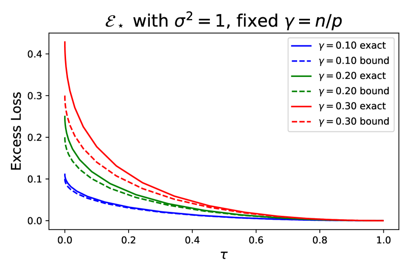
(a) For fixed $\gamma=n/p$ we plot the exact value of ${\mathcal{E}}_{\star}(\tau)$ using Eq. (22) [solid] and the lower bound from Eq. (28) [dashed].

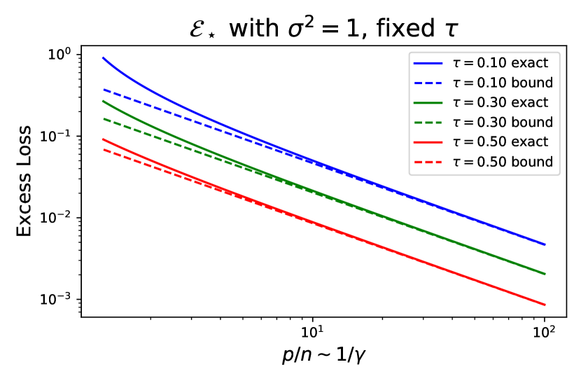
(b) For fixed $\tau$ we plot the exact value of ${\mathcal{E}}_{\star}(1/\gamma)$ using Eq. (22) [solid] and the lower bound from Eq. (28) [dashed].

Theorem 2 (MP Lower Bound).

By Theorem 1, for fixed $\tau\in[0,1]$, the minimum excess error satisfies

$${\mathcal{E}}_{\star}(\tau,\gamma)\geq\sigma^{2}\gamma(1-\sqrt{\tau})^{2}$$ (28)

for all $\gamma\in(0,+\infty)$. The dependence on $\tau$ is in fact tight since

$$\inf_{\gamma\in(0,\infty)}{\mathcal{E}}_{\star}(\tau,\gamma)/\gamma=\sigma^{2}(1-\sqrt{\tau})^{2}.$$ (29)

Proof.

Observe that as $\gamma\to 0$, the spectral eigenvalue distribution of ${\boldsymbol{W}}{\boldsymbol{W}}^{\mathsf{T}}/p$ is converging to a point mass at 1. Therefore, recalling the function $f$ defined in Eq. (26), by the Dominated Convergence Theorem

$$\lim_{\gamma\to 0}f(\lambda,\gamma)=\lim_{\gamma\to 0}\int_{s\in[1-\sqrt{\gamma},1+\sqrt{\gamma}]}\frac{\lambda^{2}}{(s+\lambda)^{2}}\differential{H}_{\gamma}(s)=\frac{\lambda^{2}}{(1+\lambda)^{2}}$$

hence by continuity

$$\lim_{\gamma\to 0}f^{-1}(\tau,\gamma)=\frac{{\color[rgb]{0,0,0}\sqrt{\tau}}}{(1-{\color[rgb]{0,0,0}\sqrt{\tau}})}.$$

Thus letting $\lambda=\lim_{\gamma\to 0}f^{-1}(\tau,\gamma)$, we get

$$\lim_{\gamma\to 0}\frac{{\mathcal{E}}_{\star}(\tau,\gamma)}{\sigma^{2}\gamma}=\lim_{\gamma\to 0}\int_{s\in[1-\sqrt{\gamma},1+\sqrt{\gamma}]}\frac{s}{(s+\lambda)^{2}}\differential{H}_{\gamma}(s)=\frac{1}{(1+\lambda)^{2}}=(1-{\color[rgb]{0,0,0}\sqrt{\tau}})^{2}.$$

By Eq. (28), we have that the limit equals the infimum

$$\lim_{\gamma\to 0}\frac{{\mathcal{E}}_{\star}(\tau,\gamma)}{\sigma^{2}\gamma}=\inf_{\gamma\in(0,\infty)}\frac{{\mathcal{E}}_{\star}(\tau,\gamma)}{\sigma^{2}\gamma}$$

which shows Eq. (29). ∎

From the above Theorem 2 we saw that ${\mathcal{E}}_{\star}(\tau,\gamma)/\gamma\to(1-\sqrt{\tau})^{2}$ as $\gamma\to 0$, achieving its infimum in the limit. In the following theorem we will show that moreover ${\mathcal{E}}_{\star}(\tau,\gamma)/\gamma$ is strictly increasing in $\gamma$ which implies in particular that Eq. (28) becomes strictly looser as $\gamma$ grows.

Theorem 3.

For fixed $\tau\in(0,1]$, the ratio of the minimum excess error ${\mathcal{E}}_{\star}(\tau,\gamma)$ to $\gamma$ is increasing in $\gamma$, that is

$${\color[rgb]{0,0,0}\derivative{{\mathcal{E}}_{\star}(\tau,\gamma)/\gamma}{\gamma}=\sigma^{2}}\derivative{E(f^{-1}(\tau,\gamma),\gamma)}{\gamma}\;{\color[rgb]{0,0,0}>}\;0,\;{\color[rgb]{0,0,0}\gamma\in(0,+\infty)}$$

where the function $E$ is defined in Eq. (25).

Proof.

Let $\lambda=f^{-1}(\tau,\gamma)$. By the chain rule

$$\derivative{E(f^{-1}(\tau,\gamma),\gamma)}{\gamma}=\partialderivative{E(\lambda,\gamma)}{\gamma}+\partialderivative{E(\lambda,\gamma)}{\lambda}\partialderivative{f^{-1}(\tau,\gamma)}{\gamma}.$$ (30)

We will compute the following three terms in Eq. (30)

$$(1):~{}~{}\partialderivative{E(\lambda,\gamma)}{\gamma},~{}~{}~{}~{}(2):~{}~{}\partialderivative{E(\lambda,\gamma)}{\lambda},~{}~{}~{}~{}(3):~{}~{}\partialderivative{f^{-1}(\tau,\gamma)}{\gamma}.$$

The computation of the first two terms is direct

$$\partialderivative{E(\lambda,\gamma)}{\gamma} =\partialderivative{m(-\lambda;\gamma)}{\gamma}-\lambda\partialderivative{m^{\prime}(-\lambda;\gamma)}{\gamma},$$

$$\partialderivative{E(\lambda,\gamma)}{\lambda} =-2m^{\prime}(-\lambda;\gamma)+\lambda m^{\prime\prime}(-\lambda;\gamma).$$

For the third term, we take the derivative with respect to $\gamma$ on both sides of Eq. (27) which yields

$$\partialderivative{f(\lambda,\gamma)}{\lambda}\partialderivative{f^{-1}(\tau,\gamma)}{\gamma}+\partialderivative{f(\lambda,\gamma)}{\gamma}=0.$$

Hence after re-arranging we have

$$\partialderivative{f^{-1}(\tau,\gamma)}{\gamma}=-\frac{\partialderivative{f(\lambda,\gamma)}{\gamma}}{\partialderivative{f(\lambda,\gamma)}{\lambda}}=-\frac{\lambda^{2}\partialderivative{m^{\prime}(-\lambda;\gamma)}{\gamma}}{2\lambda m^{\prime}(-\lambda;\gamma)-\lambda^{2}m^{\prime\prime}(-\lambda;\gamma)}.$$

Computing the product of terms (2) and (3) gives

$$\partialderivative{E(\lambda,\gamma)}{\lambda}\partialderivative{f^{-1}(\tau,\gamma)}{\gamma}=\lambda\partialderivative{m^{\prime}(-\lambda;\gamma)}{\gamma}.$$

Finally putting everything together in Eq. (30) yields

$$\derivative{E(f^{-1}(\tau,\gamma),\gamma)}{\gamma} =\partialderivative{E(\lambda,\gamma)}{\gamma}+\partialderivative{E(\lambda,\gamma)}{\lambda}\partialderivative{f^{-1}(\tau,\gamma)}{\gamma}$$

$$=\partialderivative{m(-\lambda;\gamma)}{\gamma}-\lambda\partialderivative{m^{\prime}(-\lambda;\gamma)}{\gamma}+\lambda\partialderivative{m^{\prime}(-\lambda;\gamma)}{\gamma}$$

$$=\partialderivative{m(-\lambda;\gamma)}{\gamma}\Bigg{|}_{\lambda=f^{-1}(\tau,\gamma)}\,{\color[rgb]{0,0,0}>}\,0,$$

where the last inequality follows from Lemma 10. ∎

The previous bound provides a lower bound on the minimum excess risk that holds for all $\tau\in[0,1]$ and becomes tight as $\gamma\to 0$ i.e. the amount of overparametrization becomes large. However, the bound is loose for small $\tau$ near the interpolation peak $\gamma=1$. To understand behavior in this regime, for a fixed $\gamma$ we compute a local expansion of ${\mathcal{E}}_{\star}(\tau,\gamma)$ around ${\mathcal{E}}_{\star}(0,\gamma)$. Instead of directly analyzing the function ${\mathcal{E}}_{\star}(\tau,\gamma)$, we work with the function $\sqrt{{\mathcal{E}}_{\star}(t,\gamma)}$ where we re-parametrize in terms of $t:=\sqrt{\tau}$. We then obtain the bound by taking the first-order Taylor expansion of this function around $t=0$ and then arguing it is a lower bound by showing the function is convex. In the end we convert this into lower bound on the original function ${\mathcal{E}}_{\star}(\tau,\gamma)$. It is important to re-parametrize in terms of $\sqrt{\tau}$ since the derivative of ${\mathcal{E}}_{\star}(\tau,\gamma)$ with respect to $\tau$ at $0$ is $-\infty$, as is also true for the lower bound in Eq. (28). Intriguingly, as we explain in Remark 8, taking the Taylor expansion of the square-root of ${\mathcal{E}}_{\star}$ yields a tighter approximation rather than directly expanding ${\mathcal{E}}_{\star}$.

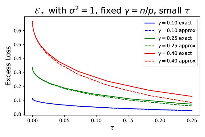
Figure 2: For fixed $\gamma=n/p$ we plot the exact value of ${\mathcal{E}}_{\star}(\tau)$ using Eq. (22) [solid] and the first-order Taylor approximation around $\tau=0$ from Eq. 31 [dashed]. Observe that as $\gamma\to 1$ the approximation becomes less tight for larger values of $\tau$.

Theorem 4 (MP lower bound for small $\tau$).

For fixed $\gamma\in(0,1)$ and $\tau\in[0,1-\gamma]$ we have

$${\mathcal{E}}_{\star}(\tau,\gamma)\geq\frac{\sigma^{2}\gamma}{1-\gamma}\quantity(1-\frac{\sqrt{\tau}}{\sqrt{1-\gamma}})^{2}.$$ (31)

Moreover, the lower bound is tight up to $o(\sqrt{\tau})$ error.

Proof.

In the proof we will often suppress the dependence on $\gamma$ and express dependence on $\tau$ in terms of $t:=\sqrt{\tau}$. In particular, recalling the functions $E$, $f$, and $f^{-1}$ defined in Eqs. (25), (26), and (27) we use

$${\mathcal{E}}_{\star}(t) :={\mathcal{E}}_{\star}(\tau,\gamma),~{}~{}~{}~{}f^{-1}(t) :=f^{-1}(\tau,\gamma)$$

$$E(\lambda) :=E(\lambda,\gamma),~{}~{}~{}~{}f(\lambda) :=f(\lambda,\gamma),$$

and as a result Eq. (27) becomes

$$f(f^{-1}(t))=t^{2}.$$ (32)

The first-order Taylor approximation of $\sqrt{{\mathcal{E}}_{\star}(t)}$ around $t=0$ is given by

$$P_{1}(t):=\sqrt{{\mathcal{E}}_{\star}(0)}+t\cdot\derivative{t}\sqrt{{\mathcal{E}}_{\star}(t)}\Bigr{|}_{t=0}=\sqrt{{\mathcal{E}}_{\star}(0)}+\frac{t}{2\sqrt{{\mathcal{E}}_{\star}(0)}}\cdot{\mathcal{E}}_{\star}^{\prime}(0).$$ (33)

where as $t\to 0^{+}$

$$\sqrt{{\mathcal{E}}_{\star}(t)}=P_{1}(t)+o(t).$$ (34)

Note that since $\lim_{t\to 0^{+}}f^{-1}(t,\gamma)=0$ for any $\gamma$, by Lemma 8 we

$${\mathcal{E}}_{\star}(0)=\sigma^{2}\gamma\lim_{\lambda\to 0^{+}}[m(-\lambda;\gamma)-\lambda m^{\prime}(-\lambda;\gamma)]=\sigma^{2}\gamma\lim_{\lambda\to 0^{+}}m(-\lambda;\gamma)=\frac{\sigma^{2}\gamma}{1-\gamma}.$$

Furthermore letting $\lambda=f^{-1}(t)$, we have by the chain rule

$${\mathcal{E}}_{\star}^{\prime}(t)=\sigma^{2}\gamma\derivative{E(f^{-1}(t))}{t}=\sigma^{2}\gamma\derivative{E(\lambda)}{\lambda}\derivative{f^{-1}(t)}{t}.$$ (35)

We can directly calculate the first term

$$\derivative{E(\lambda)}{\lambda}=-2m(-\lambda;\gamma)+\lambda m^{\prime\prime}(-\lambda;\gamma).$$

By differentiating both sides of Eq. (32) with respect to $t$ we get

$$\derivative{f^{-1}(t)}{t}\derivative{f(\lambda)}{\lambda}=2t.$$

Therefore rearranging the above gives

$$\derivative{f^{-1}(t)}{t}=\frac{2t}{f^{\prime}(\lambda)} =\frac{2t}{2\lambda m^{\prime}(-\lambda;\gamma)-\lambda^{2}m^{\prime\prime}(-\lambda;\gamma)}$$

$$=\frac{2\lambda\sqrt{m^{\prime}(-\lambda;\gamma)}}{2\lambda m^{\prime}(-\lambda;\gamma)-\lambda^{2}m^{\prime\prime}(-\lambda;\gamma)}$$

$$=\frac{2\sqrt{m^{\prime}(-\lambda;\gamma)}}{2m^{\prime}(-\lambda;\gamma)-\lambda m^{\prime\prime}(-\lambda;\gamma)}.$$

Hence from Eq. (35) we see

$${\mathcal{E}}_{\star}^{\prime}(t)=-2\sigma^{2}\gamma\sqrt{m^{\prime}(-\lambda,\gamma)}.$$ (36)

Observe that since $m^{\prime}(-\lambda;\gamma)\geq 0$, the derivative ${\mathcal{E}}_{\star}^{\prime}(t)\leq 0$. Furthermore, since $\lambda$ is increasing in $t$ and $m^{\prime}(-\lambda;\gamma)$ is decreasing in $\lambda$, it follows that $m^{\prime}(-\lambda;\gamma)$ is decreasing in $t$. Thus ${\mathcal{E}}_{\star}^{\prime}(t)$ is increasing, i.e. ${\mathcal{E}}_{\star}^{\prime\prime}(t)\geq 0$. Using Lemma 9

$${\mathcal{E}}_{\star}^{\prime}(0)=\lim_{\lambda\to 0^{+}}-2\sigma^{2}\gamma\sqrt{m^{\prime}(-\lambda,\gamma)}=-2\gamma\sigma^{2}\frac{1}{(1-\gamma)^{3/2}}.$$

Plugging this into the Taylor approximation $P_{1}(t)$ in Eq. (33) we get that

$$P_{1}(t) =\sigma\sqrt{\frac{\gamma}{1-\gamma}}-\sigma t\sqrt{\frac{1-\gamma}{\gamma}}\frac{\gamma}{(1-\gamma)^{3/2}}$$

$$=\sigma\sqrt{\frac{\gamma}{1-\gamma}}\quantity(1-t\frac{1}{\sqrt{1-\gamma}}).$$

We now show that $\sqrt{{\mathcal{E}}_{\star}(t)}\geq P_{1}(t)$ by showing that $\sqrt{{\mathcal{E}}_{\star}(t)}$ is convex on $[0,1]$ for which it suffices to show that the second derivative is non-negative. Computing the second derivative, we get

$$\derivative[2]{t}\sqrt{{\mathcal{E}}_{\star}(t)}=\frac{{\mathcal{E}}_{\star}(t)}{2\sqrt{{\mathcal{E}}_{\star}(t)}}-\frac{{\mathcal{E}}_{\star}^{\prime}(t)}{4{\mathcal{E}}_{\star}(t)^{3/2}}.$$

We can see that this is always non-negative since ${\mathcal{E}}_{\star}(t)\geq 0$ and from Eq. (36) and the accompanying remarks ${\mathcal{E}}_{\star}^{\prime}(t)\leq 0$ and ${\mathcal{E}}_{\star}^{\prime\prime}(t)\geq 0$. Returning to the original $\tau$ parameterization, we have that for all $\tau\in[0,1]$

$$\sqrt{{\mathcal{E}}_{\star}(\tau)}\geq P_{1}(\sqrt{\tau})=\sigma\sqrt{\frac{\gamma}{1-\gamma}}\quantity(1-\sqrt{\frac{\tau}{1-\gamma}}).$$

Note that for $\tau\leq 1-\gamma$, both sides of the above inequality are non-negative. Hence we can square both sides yielding

$${\mathcal{E}}_{\star}(\tau,\gamma)\geq\sigma^{2}\frac{\gamma}{1-\gamma}\quantity(1-\sqrt{\frac{\tau}{1-\gamma}})^{2}$$

which was the desired lower bound. The fact that the bound is tight up to $o(\sqrt{\tau})$ follows from Eq. (34). ∎

Remark 8.

Observe that from the above computations the first-order expansion of ${\mathcal{E}}_{\star}(t)$ is given by

$${\mathcal{E}}_{\star}(0)+\sqrt{\tau}{\mathcal{E}}_{\star}^{\prime}(0)=\sigma^{2}\sqrt{\frac{\gamma}{1-\gamma}}\quantity(1-2\sqrt{\frac{\tau}{1-\gamma}})<\sigma^{2}\frac{\gamma}{1-\gamma}\quantity(1-\sqrt{\frac{\tau}{1-\gamma}})^{2}\leq{\mathcal{E}}_{\star}(\tau)$$

which shows that expanding the square-root of the minimum excess error yields a tighter bound.

Note that the bound in Eq. (31) matches the lower bound in Theorem 2 as $\gamma\to 0$. Interestingly, this bound has the form of a multiplicative factor of the minimum interpolation $(\tau=0)$ loss and is only valid for small $\tau$. We will in fact show that no bound of that form can capture the behavior of the excess loss for arbitrarily small $\tau>0$ as $\gamma\to 1$ in Theorem 5. In particular, we now show a discontinuity at $\tau=0$ when considering the peak $n=p$.

Theorem 5 (Excess Loss at Peak).

For $\gamma=1$ and $\tau\in(0,1)$,

$$\frac{{\mathcal{E}}_{\star}(\tau,1)}{\sigma^{2}}=\frac{1}{4\tau}+\frac{\tau}{4}-\frac{1}{2}$$

hence as $\tau\to 0$,

$${\mathcal{E}}_{\star}(\tau,1)=\Theta(\tau^{-1}).$$

Proof.

Consider the Stieltjes transform $m(-z;\gamma)$ and its derivative. At the interpolation peak $\gamma=1$, we have

$$m(-z;1) =\frac{1}{2}\quantity(\sqrt{1+4/z}-1)$$

$$m^{\prime}(-z;1) =-\frac{z+2}{2z\sqrt{z^{2}+4z}}+\frac{\sqrt{z^{2}+4z}}{2z^{2}}.$$

One can then check that

$$z^{2}m^{\prime}(-z;1)=\frac{1}{\sqrt{1+4/z}}.$$

Hence the fixed point equation Eq. (23) can be written as

$$\tau=\lambda^{2}m^{\prime}(-\lambda;1)=\frac{1}{\sqrt{1+4/\lambda}}$$

which implies that $\lambda$ satisfies the following

$$\sqrt{1+4/\lambda} =\frac{1}{\tau},$$

$$\frac{1}{\lambda} =\frac{1}{4}\quantity(\frac{1}{\tau^{2}}-1).$$

Using the above relations, we can compute the minimum excess error using Eq. (22)

$$\frac{{\mathcal{E}}_{\star}(\tau,1)}{\sigma^{2}} =m(-\lambda;1)-\lambda m^{\prime}(-\lambda;1)$$

$$=\frac{1}{2}\quantity(\sqrt{1+4/\lambda}-1)-\frac{\tau}{\lambda}$$

$$=\frac{1}{2}\quantity(\frac{1}{\tau}-1)-\frac{1}{4}\quantity(\frac{1}{\tau}-\tau)$$

$$=\frac{1}{4\tau}+\frac{\tau}{4}-\frac{1}{2}.$$

∎

Remark 9.

As mentioned earlier, a consequence of the above is that we cannot have a lower bound of the form ${\mathcal{E}}_{\star}(\tau;n,p)\geq{\mathcal{E}}_{\star}(0;n,p)\cdot f(\tau)$ for some function $f$ which satisfies $f(\tau)>0$ for $\tau>0$ since for any $\tau>0$,

$$\lim_{\gamma\to 1}\frac{{\mathcal{E}}_{\star}(\tau,\gamma)}{{\mathcal{E}}_{\star}(0,\gamma)}=0.$$

4 Conclusion

In this work we demonstrated a trade-off between the expected loss, empirical loss, and the number of parameters for general linear models. In particular we have shown that near-optimal algorithms output models that are either classical (with empirical loss approaching the noise level) or have significant excess over-parameterization, i.e., have many more parameters than the number needed to fit the training data. This trade-off is universal as it is non-asymptotic, holds for any algorithm, and any data distribution (under mild non-degeneracy assumptions).

We also provided a more precise asymptotic lower bound under Marchenko-Pastur distributional assumptions near the classical double descent peak where the amount of overparametrization is just enough to interpolate the data. Remarkably however, as the level of overparametrization increases the minimum excess loss exactly matches the universal bound, demonstrating the tightness of the bound.

The open questions that remain include extending our results to more general non-linear parametric families and to classification settings.

Appendix A Missing Proofs from Section 2.1

In this section of the appendix, we supply missing proofs for some the auxiliary results used in the proof of Theorem 1 in Section 2.1. Recall that we denote the optimal linear predictor as $\beta_{\star}:=\operatorname*{arg\,min}_{{\boldsymbol{\beta}}\in\mathbb{R}^{p}}R(\beta)$.

Lemma 5 (Optimal Linear Predictor).

Define ${\boldsymbol{\beta}}_{\star}$ as in Eq. (5). Then

1. $\beta_{\star}$ is the orthogonal projection of $f_{\star}$ onto the subspace of linear functions ${\mathcal{H}}=\{\beta({\boldsymbol{x}}):{\boldsymbol{\beta}}\in\mathbb{R}^{p}\}$ in $L^{2}$,

2. ${\mathcal{E}}(f):=R(f)-R(f_{\star})=\mathbb{E}_{{\boldsymbol{x}}}[(f({\boldsymbol{x}})-f_{\star}({\boldsymbol{x}}))^{2}$,

3. ${\mathcal{E}}^{\mathrm{lin}}(\beta):=R(\beta)-R(\beta_{\star})=\mathbb{E}_{{\boldsymbol{x}}}[(\beta({\boldsymbol{x}})-\beta_{\star}({\boldsymbol{x}}))^{2}]$.

Proof.

By definition of the optimal linear predictor

$$\beta_{\star} =\operatorname*{arg\,min}_{\beta\in{\mathcal{H}}}R(\beta)$$

$$=\operatorname*{arg\,min}_{\beta\in{\mathcal{H}}}\mathbb{E}_{({\boldsymbol{x}},y)}[(y-\beta({\boldsymbol{x}}))^{2}]$$

$$=\operatorname*{arg\,min}_{\beta\in{\mathcal{H}}}\mathbb{E}_{({\boldsymbol{x}},y)}[(y-f_{\star}({\boldsymbol{x}}))^{2}+(f_{\star}({\boldsymbol{x}})-\beta({\boldsymbol{x}}))^{2}] (\text{since }\mathbb{E}_{y\mid{\boldsymbol{x}}}[y-f_{\star}({\boldsymbol{x}})]=0)$$

$$=\operatorname*{arg\,min}_{\beta\in{\mathcal{H}}}\mathbb{E}_{{\boldsymbol{x}}}[(f_{\star}({\boldsymbol{x}})-\beta({\boldsymbol{x}}))^{2}],$$

which shows Claim 1. For Claim 2

$$R(f)-R(f_{\star}) =\mathbb{E}_{({\boldsymbol{x}},y)}[(y-f({\boldsymbol{x}}))^{2}]-\mathbb{E}_{({\boldsymbol{x}},y)}[(y-f_{\star}({\boldsymbol{x}}))^{2}]$$

$$=\mathbb{E}_{({\boldsymbol{x}},y)}[(f({\boldsymbol{x}})-f_{\star}({\boldsymbol{x}}))^{2}]-2\mathbb{E}_{({\boldsymbol{x}},y)}[(f({\boldsymbol{x}})-f_{\star}({\boldsymbol{x}}))(y-f_{\star}({\boldsymbol{x}}))]$$

$$=\mathbb{E}_{{\boldsymbol{x}}}[(f({\boldsymbol{x}})-f_{\star}({\boldsymbol{x}}))^{2}].$$

For Claim 3

$$R(\beta)-R(\beta_{\star}) ={\mathcal{E}}(\beta)-{\mathcal{E}}(\beta_{\star})$$

$$=\mathbb{E}_{{\boldsymbol{x}}}[(f_{\star}({\boldsymbol{x}})-\beta({\boldsymbol{x}}))^{2}-(f_{\star}({\boldsymbol{x}})-\beta_{\star}({\boldsymbol{x}}))^{2}]$$

$$=\mathbb{E}_{{\boldsymbol{x}}}[(\beta({\boldsymbol{x}})-\beta_{\star}({\boldsymbol{x}}))^{2}]-2\mathbb{E}_{{\boldsymbol{x}}}[(f_{\star}({\boldsymbol{x}})-\beta_{\star}({\boldsymbol{x}}))(\beta({\boldsymbol{x}})-\beta_{\star}({\boldsymbol{x}}))]$$

$$=\mathbb{E}_{{\boldsymbol{x}}}[(\beta({\boldsymbol{x}})-\beta_{\star}({\boldsymbol{x}}))^{2}]$$

where the second equality holds from Claim 2 and the last equality holds from Claim 1 in Lemma 5. ∎

Lemma 6 (Excess Linear Loss).

The excess loss satisfies the following lower bound

$${\mathcal{E}}(\beta)\geq{\mathcal{E}}^{\mathrm{lin}}(\beta)=\norm{{\boldsymbol{\Sigma}}^{1/2}({\boldsymbol{\beta}}-{\boldsymbol{\beta}}_{\star})}^{2}.$$

Proof.

It is clear that ${\mathcal{E}}(\beta)\geq{\mathcal{E}}^{\mathrm{lin}}(\beta)$. Using Lemma 5 and the definition of ${\boldsymbol{\Sigma}}$

$${\mathcal{E}}(\beta) =\mathbb{E}_{{\boldsymbol{x}}}(\beta({\boldsymbol{x}})-\beta_{\star}({\boldsymbol{x}}))^{2}$$

$$=\mathbb{E}_{{\boldsymbol{x}}}({\boldsymbol{\beta}}^{\mathsf{T}}\phi({\boldsymbol{x}})-{\boldsymbol{\beta}}_{\star}^{\mathsf{T}}\phi({\boldsymbol{x}}))^{2}$$

$$=({\boldsymbol{\beta}}-{\boldsymbol{\beta}}_{\star})^{\mathsf{T}}\mathbb{E}_{{\boldsymbol{x}}}[\phi({\boldsymbol{x}})\phi({\boldsymbol{x}})^{\mathsf{T}}]({\boldsymbol{\beta}}-{\boldsymbol{\beta}}_{\star})$$

$$=\norm{{\boldsymbol{\Sigma}}^{1/2}({\boldsymbol{\beta}}-{\boldsymbol{\beta}}_{\star})}^{2}.$$

∎

Recall that we defined the random vectors

$${\boldsymbol{\xi}}_{\mathrm{noise}}=(y_{i}-f_{\star}({\boldsymbol{x}}_{i}))_{i\in[n]}\in\mathbb{R}^{n},~{}~{}~{}~{}{\boldsymbol{\xi}}_{\mathrm{lin}}=(f_{\star}({\boldsymbol{x}}_{i})-\beta_{\star}({\boldsymbol{x}}_{i}))_{i\in[n]}\in\mathbb{R}^{n}$$

and let ${\boldsymbol{\xi}}={\boldsymbol{\xi}}_{\mathrm{noise}}+{\boldsymbol{\xi}}_{\mathrm{lin}}$.

Lemma 7 (Expectation Over Noise).

Let $f:\mathbb{R}^{n\times d}\to\mathbb{S}^{n}_{+}$ be any PSD matrix valued function. Then,

$$\mathbb{E}_{{\boldsymbol{y}},{\boldsymbol{X}}}[{\boldsymbol{\xi}}^{\mathsf{T}}f({\boldsymbol{X}}){\boldsymbol{\xi}}]\geq\sigma^{2}\mathbb{E}_{{\boldsymbol{X}}}\Tr(f({\boldsymbol{X}})).$$ (37)

Moreover, if $\text{Var}(y\,|\,{\boldsymbol{x}})=\sigma^{2}$ almost surely and $f_{\star}=\beta_{\star}$ then the above is an equality.

Proof.

Recalling that ${\boldsymbol{\xi}}={\boldsymbol{\xi}}_{\mathrm{noise}}+{\boldsymbol{\xi}}_{\mathrm{lin}}$. By definition of ${\boldsymbol{\xi}}_{\mathrm{noise}}$ we have that

$$\mathbb{E}_{{\boldsymbol{y}}\mid{\boldsymbol{X}}}[{\boldsymbol{\xi}}_{\mathrm{noise}}]={\boldsymbol{0}}$$

and by the assumption on the noise variance we have almost surely

$$\mathbb{E}_{{\boldsymbol{y}}\mid{\boldsymbol{X}}}[{\boldsymbol{\xi}}_{\mathrm{noise}}{\boldsymbol{\xi}}_{\mathrm{noise}}^{\mathsf{T}}]=\text{diag}((\text{Var}[y\mid{\boldsymbol{x}}_{i}])_{i\in[n]})\succeq\sigma^{2}{\mathbf{I}}.$$ (38)

Using these observations we have

$$\mathbb{E}_{{\boldsymbol{y}}\mid{\boldsymbol{X}}}[{\boldsymbol{\xi}}^{\mathsf{T}}f({\boldsymbol{X}}){\boldsymbol{\xi}}] =\mathbb{E}_{{\boldsymbol{y}}\mid{\boldsymbol{X}}}[{\boldsymbol{\xi}}_{\mathrm{noise}}^{\mathsf{T}}f({\boldsymbol{X}}){\boldsymbol{\xi}}_{\mathrm{noise}}]+2\mathbb{E}_{{\boldsymbol{y}}\mid{\boldsymbol{X}}}[{\boldsymbol{\xi}}_{\mathrm{lin}}^{\mathsf{T}}f({\boldsymbol{X}}){\boldsymbol{\xi}}_{\mathrm{noise}}]+\mathbb{E}_{{\boldsymbol{y}}\mid{\boldsymbol{X}}}[{\boldsymbol{\xi}}_{\mathrm{lin}}^{\mathsf{T}}f({\boldsymbol{X}}){\boldsymbol{\xi}}_{\mathrm{lin}}]$$

$$=\Tr(f({\boldsymbol{X}})\mathbb{E}_{{\boldsymbol{y}}\mid{\boldsymbol{X}}}[{\boldsymbol{\xi}}_{\mathrm{noise}}{\boldsymbol{\xi}}_{\mathrm{noise}}^{\mathsf{T}}])+2{\boldsymbol{\xi}}_{\mathrm{lin}}^{\mathsf{T}}f({\boldsymbol{X}})\mathbb{E}_{{\boldsymbol{y}}\mid{\boldsymbol{X}}}[{\boldsymbol{\xi}}_{\mathrm{noise}}]+{\boldsymbol{\xi}}_{\mathrm{lin}}^{\mathsf{T}}f({\boldsymbol{X}}){\boldsymbol{\xi}}_{\mathrm{lin}}$$

$$=\Tr(f({\boldsymbol{X}})\mathbb{E}_{{\boldsymbol{y}}\mid{\boldsymbol{X}}}[{\boldsymbol{\xi}}_{\mathrm{noise}}{\boldsymbol{\xi}}_{\mathrm{noise}}^{\mathsf{T}}])+{\boldsymbol{\xi}}_{\mathrm{lin}}^{\mathsf{T}}f({\boldsymbol{X}}){\boldsymbol{\xi}}_{\mathrm{lin}}$$

$$\geq\sigma^{2}\Tr(f({\boldsymbol{X}}))+{\boldsymbol{\xi}}_{\mathrm{lin}}^{\mathsf{T}}f({\boldsymbol{X}}){\boldsymbol{\xi}}_{\mathrm{lin}}$$

$$\geq\sigma^{2}\Tr(f({\boldsymbol{X}})),$$

where we used Eq. (38) in the first inequality and we used the assumption that $f({\boldsymbol{X}})$ is a PSD matrix for the last inequality. By iterating expectations we have

$$\mathbb{E}_{{\boldsymbol{y}},{\boldsymbol{X}}}[{\boldsymbol{\xi}}^{\mathsf{T}}f({\boldsymbol{X}}){\boldsymbol{\xi}}]=\mathbb{E}_{{\boldsymbol{X}}}\mathbb{E}_{{\boldsymbol{y}}\mid{\boldsymbol{X}}}[{\boldsymbol{\xi}}^{\mathsf{T}}f({\boldsymbol{X}}){\boldsymbol{\xi}}]\geq\sigma^{2}\mathbb{E}_{{\boldsymbol{X}}}\Tr(f({\boldsymbol{X}}))$$

as desired. Note that if $\text{Var}(y\,|\,{\boldsymbol{x}})=\sigma^{2}$ then Eq. (38) becomes an equality and if $f_{\star}=\beta_{\star}$ then ${\boldsymbol{\xi}}_{\mathrm{lin}}={\boldsymbol{0}}$ and so it easy to see that Eq. (37) is an equality as well. ∎

Appendix B Marchenko-Pastur Law

In this section, we will give some definitions, facts, and results concerning the Marchenko-Pastur Law.

Definition 1 (Marchenko-Pastur Law).

The Marchenko-Pastur Law with aspect ratio $\gamma$, denoted $\mathsf{MP}(\gamma)$, is given the probability distribution

$$\quantity(1-\frac{1}{\gamma})_{+}\delta_{0}+\frac{1}{\gamma 2\pi x}\sqrt{(b-x)(x-a)}$$

where

$$a=(1-\sqrt{\gamma}){\color[rgb]{0,0,0}{}^{2}},~{}~{}~{}~{}b=(1+\sqrt{\gamma}){\color[rgb]{0,0,0}{}^{2}}.$$

Definition 2 (Stieltjes Transform).

For $z>0$ and $\gamma>0$, the Stieltjes transform of the Marchenko-Pastur law is

$$m(-z;\gamma):=\int\frac{1}{s+z}\differential{\mathsf{MP}_{\gamma}(s)}=\frac{-(1-\gamma+z)+\sqrt{(1-\gamma+z)^{2}+4\gamma z}}{2\gamma z}$$

and its derivative satisfies

$$m^{\prime}(-z;\gamma) =\int\frac{1}{(s+z)^{2}}\differential{\mathsf{MP}_{\gamma}(s)}$$

$$=\frac{-(1-\gamma+z)-2\gamma}{2\gamma z\sqrt{(1-\gamma+z)^{2}+4\gamma z}}+\frac{1}{2\gamma z}+\frac{\sqrt{(1-\gamma+z)^{2}+4\gamma z}-(1-\gamma+z)}{2z^{2}\gamma}.$$

Lemma 8.

For any $\gamma>0$,

$$\lim_{z\to 0^{+}}m(-z;\gamma)=\frac{1}{1-\gamma}$$

Proof.

This just follows from a direct computation

$$\lim_{z\to 0^{+}}m(-z;\gamma) =\lim_{z\to 0^{+}}\frac{-(1-\gamma+z)+\sqrt{(1-\gamma+z)^{2}+4\gamma z}}{2\gamma z}$$

$$=\lim_{z\to 0^{+}}\frac{-(1-\gamma+z)^{2}+(1-\gamma+z)^{2}+4\gamma z}{2\gamma z[(1-\gamma+z)+\sqrt{(1-\gamma+z)^{2}+4\gamma z}]}$$

$$=\lim_{z\to 0^{+}}\frac{2}{(1-\gamma+z)+\sqrt{(1-\gamma+z)^{2}+4\gamma z}}=\frac{1}{1-\gamma}.$$

∎

Lemma 9.

For any $\gamma>0$,

$$\lim_{z\to 0^{+}}m^{\prime}(-z;\gamma)=\frac{1}{(1-\gamma)^{3}}$$

Proof.

By the definition of derivative

$$\lim_{z\to 0^{+}}m^{\prime}(-z;\gamma) =\lim_{z\to 0^{+}}\frac{m(-z;\gamma)-m(0;\gamma)}{-z}$$

$$=\lim_{z\to 0^{+}}\frac{1}{z}\quantity(\frac{(1-\gamma+z)-\sqrt{(1-\gamma+z)^{2}+4\gamma z}}{2\gamma z}+\frac{1}{1-\gamma})$$

$$=\lim_{z\to 0^{+}}\frac{(1-\gamma)(1-\gamma+z)-(1-\gamma)\sqrt{(1-\gamma+z)^{2}+4\gamma z}+2\gamma z}{2\gamma(1-\gamma)z^{2}}$$

$$=\lim_{z\to 0^{+}}\frac{(1-\gamma)^{2}+z(1+\gamma)-(1-\gamma)\sqrt{(1-\gamma+z)^{2}+4\gamma z}}{2\gamma(1-\gamma)z^{2}}$$

$$=\lim_{z\to 0^{+}}\frac{[(1-\gamma)^{2}+z(1+\gamma)]^{2}-(1-\gamma)^{2}[(1-\gamma+z)^{2}+4\gamma z]}{2\gamma(1-\gamma)z^{2}[(1-\gamma)^{2}+z(1+\gamma)+(1-\gamma)\sqrt{(1-\gamma+z)^{2}+4\gamma z}]}$$

Observe that the numerator simplifies as

$$[(1-\gamma)^{2}+z(1+\gamma)]^{2}-(1-\gamma)^{2}[(1-\gamma+z)^{2}+4\gamma z]$$

$$=(1-\gamma)^{4}+2z(1-\gamma)^{2}(1+\gamma)+z^{2}(1+\gamma)^{2}-[(1-\gamma)^{4}+2z(1-\gamma)^{2}(1+\gamma)+(1-\gamma)^{2}z^{2}]$$

$$=z^{2}[(1+\gamma)^{2}-(1-\gamma)^{2}]=4z^{2}\gamma.$$

Hence

$$\lim_{z\to 0^{+}}m^{\prime}(-z;\gamma) =\lim_{z\to 0^{+}}\frac{4\gamma}{2\gamma(1-\gamma)[(1-\gamma)^{2}+z(1+\gamma)+(1-\gamma)\sqrt{(1-\gamma+z)^{2}+4\gamma z}]}$$

$$=\frac{2}{(1-\gamma)[(1-\gamma)^{2}+(1-\gamma)\sqrt{(1-\gamma)^{2}}]}=\frac{1}{(1-\gamma)^{3}}.$$

∎

Lemma 10.

For any $z>0$,

$$\partialderivative{m(-z;\gamma)}{\gamma}\,{\color[rgb]{0,0,0}>}\,0.$$

Proof.

We can rewrite the Stieltjes transform as follows

$$m(-z;\gamma) =\frac{-(1-\gamma+z)+\sqrt{(1-\gamma+z)^{2}+4\gamma z}}{2\gamma z}$$

$$=\frac{-(1-\gamma+z)+\sqrt{(1-\gamma+z)^{2}+4\gamma z}}{2\gamma z}\frac{(1-\gamma+z)+\sqrt{(1-\gamma+z)^{2}+4\gamma z}}{(1-\gamma+z)+\sqrt{(1-\gamma+z)^{2}+4\gamma z}}$$

$$=\frac{2}{(1-\gamma+z)+\sqrt{(1-\gamma+z)^{2}+4\gamma z}}.$$

Therefore it suffices to show that

$$f(\gamma)=(1-\gamma+z)+\sqrt{(1-\gamma+z)^{2}+4\gamma z}$$

is decreasing in $\gamma$. Taking the derivative we see that

$$f^{\prime}(\gamma)=-1+\frac{-(1-\gamma+z)+2z}{\sqrt{(1-\gamma+z)^{2}+4\gamma z}}.$$

Note that $f^{\prime}(\gamma)\,{\color[rgb]{0,0,0}<}\,0$ if and only if

$$2z-(1-\gamma+z)\,{\color[rgb]{0,0,0}<}\,\sqrt{(1-\gamma+z)^{2}+4\gamma z}.$$

Squaring both sides and clearing terms this is equivalent to

$$4z^{2}-4z(1-\gamma+z)\,{\color[rgb]{0,0,0}<}\,4\gamma z.$$

Using the fact that $z>0$ we can divide both sides by $4z$ to get

$$z-(1-\gamma+z)\,{\color[rgb]{0,0,0}<}\,\gamma$$

which is clearly true. ∎

Appendix C Auxiliary Lemmas

Lemma 11 (AM-HM inequality).

Let $x_{1},\ldots,x_{n}\in\mathbb{R}$. Then

$$\sum\limits_{i=1}^{n}\frac{1}{x_{i}}\geq n^{2}\quantity(\sum\limits_{i=1}^{n}x_{i})^{-1}.$$

Proof.

By the Cauchy-Schwarz inequality

$$n^{2}=\quantity(\sum\limits_{i=1}^{n}\sqrt{x_{i}}\cdot\frac{1}{\sqrt{x_{i}}})^{2}\leq\sum\limits_{i=1}^{n}\sqrt{x_{i}}^{2}\cdot\sum\limits_{i=1}^{n}\frac{1}{\sqrt{x_{i}}^{2}},$$

which after re-arranging gives the desired inequality. ∎

Lemma 12 (Chebyshev’s Sum Inequality [33]).

If $a_{1}\leq a_{2}\leq\ldots\leq a_{n}$ and $b_{1}\geq\ldots\geq b_{n}$ then

$$\frac{1}{n}\sum\limits_{i=1}^{n}a_{i}b_{i}\leq\quantity(\frac{1}{n}\sum\limits_{i=1}^{n}a_{i})\quantity(\frac{1}{n}\sum\limits_{i=1}^{n}b_{i}).$$

Lemma 13 (Concentration of Quadratic Forms, Lemma 7.6 from [32]).

For each positive integer $n$, let ${\boldsymbol{A}}_{n}$ be a random $n\times n$ PSD matrix. Let $\xi_{1},\xi_{2},\ldots$ be a sequence of i.i.d random variables and denote ${\boldsymbol{\xi}}_{n}=(\xi_{1},\ldots,\xi_{n})$. Then if

• $\sup_{n}\norm{{\boldsymbol{A}}_{n}}=O(1)$

• $\mathbb{E}[\xi_{1}]=0$, $\mathbb{E}[\xi_{1}^{2}]=\sigma^{2}$, and $\mathbb{E}[\xi_{1}^{4+\eta}]$ for some $\eta>0$

we have the following convergence

$$\frac{1}{n}{\boldsymbol{\xi}}_{n}^{\mathsf{T}}{\boldsymbol{A}}_{n}{\boldsymbol{\xi}}_{n}-\frac{\sigma^{2}}{n}\Tr({\boldsymbol{A}}_{n})\to 0$$

almost surely.

References

- [1] Peter L Bartlett, Philip M Long, Gábor Lugosi, and Alexander Tsigler. Benign overfitting in linear regression. Proceedings of the National Academy of Sciences, 117(48):30063–30070, 2020.
- [2] Vidya Muthukumar, Kailas Vodrahalli, Vignesh Subramanian, and Anant Sahai. Harmless interpolation of noisy data in regression. IEEE Journal on Selected Areas in Information Theory, 1(1):67–83, 2020.
- [3] Luc Devroye, Laszlo Györfi, and Adam Krzyżak. The hilbert kernel regression estimate. Journal of Multivariate Analysis, 65(2):209–227, 1998.
- [4] Mikhail Belkin, Daniel J Hsu, and Partha Mitra. Overfitting or perfect fitting? risk bounds for classification and regression rules that interpolate. Advances in neural information processing systems, 31, 2018.
- [5] Mikhail Belkin, Alexander Rakhlin, and Alexandre B Tsybakov. Does data interpolation contradict statistical optimality? In The 22nd International Conference on Artificial Intelligence and Statistics, pages 1611–1619. PMLR, 2019.
- [6] Julien Chhor, Suzanne Sigalla, and Alexandre B Tsybakov. Benign overfitting and adaptive nonparametric regression. arXiv preprint arXiv:2206.13347, 2022.
- [7] Trevor Hastie, Andrea Montanari, Saharon Rosset, and Ryan J Tibshirani. Surprises in high-dimensional ridgeless least squares interpolation. The Annals of Statistics, 50(2):949–986, 2022.
- [8] Mikhail Belkin, Daniel Hsu, and Ji Xu. Two models of double descent for weak features. SIAM Journal on Mathematics of Data Science, 2(4):1167–1180, 2020.
- [9] Frederic Koehler, Lijia Zhou, Danica J Sutherland, and Nathan Srebro. Uniform convergence of interpolators: Gaussian width, norm bounds and benign overfitting. Advances in Neural Information Processing Systems, 34:20657–20668, 2021.
- [10] Alexander Tsigler and Peter L Bartlett. Benign overfitting in ridge regression. arXiv preprint arXiv:2009.14286, 2020.
- [11] Niladri S Chatterji and Philip M Long. Foolish crowds support benign overfitting. Journal of Machine Learning Research, 23(125):1–12, 2022.
- [12] Difan Zou, Jingfeng Wu, Vladimir Braverman, Quanquan Gu, and Sham Kakade. Benign overfitting of constant-stepsize sgd for linear regression. In Conference on Learning Theory, pages 4633–4635. PMLR, 2021.
- [13] Song Mei and Andrea Montanari. The generalization error of random features regression: Precise asymptotics and the double descent curve. Communications on Pure and Applied Mathematics, 75(4):667–766, 2022.
- [14] Song Mei, Theodor Misiakiewicz, and Andrea Montanari. Generalization error of random feature and kernel methods: hypercontractivity and kernel matrix concentration. Applied and Computational Harmonic Analysis, 59:3–84, 2022.
- [15] Tengyuan Liang and Alexander Rakhlin. Just interpolate: Kernel “ridgeless” regression can generalize. The annals of statistics, 2020.
- [16] Ben Adlam and Jeffrey Pennington. The neural tangent kernel in high dimensions: Triple descent and a multi-scale theory of generalization. In International Conference on Machine Learning, pages 74–84. PMLR, 2020.
- [17] Yuan Cao, Zixiang Chen, Mikhail Belkin, and Quanquan Gu. Benign overfitting in two-layer convolutional neural networks. arXiv preprint arXiv:2202.06526, 2022.
- [18] Spencer Frei, Niladri S Chatterji, and Peter L Bartlett. Benign overfitting without linearity: Neural network classifiers trained by gradient descent for noisy linear data. arXiv preprint arXiv:2202.05928, 2022.
- [19] Spencer Frei, Gal Vardi, Peter L Bartlett, and Nathan Srebro. Benign overfitting in linear classifiers and leaky relu networks from kkt conditions for margin maximization. arXiv preprint arXiv:2303.01462, 2023.
- [20] Zhu Li, Zhi-Hua Zhou, and Arthur Gretton. Towards an understanding of benign overfitting in neural networks. arXiv preprint arXiv:2106.03212, 2021.
- [21] Rishi Bommasani, Drew A Hudson, Ehsan Adeli, Russ Altman, Simran Arora, Sydney von Arx, Michael S Bernstein, Jeannette Bohg, Antoine Bosselut, Emma Brunskill, et al. On the opportunities and risks of foundation models. arXiv preprint arXiv:2108.07258, 2021.
- [22] Mikhail Belkin, Daniel Hsu, Siyuan Ma, and Soumik Mandal. Reconciling modern machine-learning practice and the classical bias–variance trade-off. Proceedings of the National Academy of Sciences, 116(32):15849–15854, 2019.
- [23] David Holzmüller. On the universality of the double descent peak in ridgeless regression. arXiv preprint arXiv:2010.01851, 2020.
- [24] Ingo Steinwart and Andreas Christmann. Support vector machines. Springer Science & Business Media, 2008.
- [25] Alexandre B. Tsybakov. Introduction to Nonparametric Estimation. Springer series in statistics. Springer, 2009.
- [26] Ali Rahimi and Benjamin Recht. Random features for large-scale kernel machines. Advances in neural information processing systems, 20, 2007.
- [27] Chen Cheng, John Duchi, and Rohith Kuditipudi. Memorize to generalize: on the necessity of interpolation in high dimensional linear regression. arXiv preprint arXiv:2202.09889, 2022.
- [28] Vitaly Feldman. Does learning require memorization? a short tale about a long tail. In Proceedings of the 52nd Annual ACM SIGACT Symposium on Theory of Computing, pages 954–959, 2020.
- [29] Gavin Brown, Mark Bun, Vitaly Feldman, Adam Smith, and Kunal Talwar. When is memorization of irrelevant training data necessary for high-accuracy learning? In Proceedings of the 53rd Annual ACM SIGACT Symposium on Theory of Computing, pages 123–132, 2021.
- [30] Sebastien Bubeck and Mark Sellke. A universal law of robustness via isoperimetry. In M. Ranzato, A. Beygelzimer, Y. Dauphin, P.S. Liang, and J. Wortman Vaughan, editors, Advances in Neural Information Processing Systems, volume 34, pages 28811–28822. Curran Associates, Inc., 2021.
- [31] Lee H Dicker. Ridge regression and asymptotic minimax estimation over spheres of growing dimension. 2016.
- [32] Edgar Dobriban and Stefan Wager. High-dimensional asymptotics of prediction: Ridge regression and classification. The Annals of Statistics, 46(1):247–279, 2018.
- [33] Godfrey Harold Hardy, John Edensor Littlewood, George Pólya, György Pólya, et al. Inequalities. Cambridge university press, 1952.