Cluster structures on braid varieties

Abstract.

We show the existence of cluster $\mathcal{A}$-structures and cluster Poisson structures on any braid variety, for any simple Lie group. The construction is achieved via weave calculus and a tropicalization of Lusztig’s coordinates. Several explicit seeds are provided and the quiver and cluster variables are readily computable. We prove that these upper cluster algebras equal their cluster algebras, show local acyclicity, and explicitly determine their DT-transformations as the twist automorphisms of braid varieties. The main result also resolves the conjecture of B. Leclerc on the existence of cluster algebra structures on the coordinate rings of open Richardson varieties.

1. Introduction

The object of this article will be to show the existence of cluster $\mathrm{K}_{2}$-structures and cluster Poisson structures on braid varieties for any simple algebraic Lie group. The construction of such cluster structures is achieved via the study of Demazure weaves and their cycles. The initial seed is explicitly obtained by using the weave and a tropicalization of Lie group identities in Lusztig’s coordinates, yielding both a readily computable exchange matrix and an initial set of cluster $\mathcal{A}$-variables. In particular, a conjecture of B. Leclerc on open Richardson varieties is resolved. We also establish general properties of these cluster structures for braid varieties, including local acyclicity and the explicit construction of a Donaldson-Thomas transformation.

1.1. Scientific Context

Cluster algebras, introduced by S. Fomin and A. Zelevinsky [2, 30, 31] in the study of Lie groups, are commutative rings endowed with a set of distinguished generators satisfying remarkable combinatorial and geometric properties. Cluster varieties, a geometric enrichment of cluster algebras introduced by V. Fock and A. Goncharov [24, 25, 26], are algebraic varieties equipped with an atlas of toric charts whose transition maps obey certain combinatorial rules, closely related to the rules of mutation in a cluster algebra. Cluster varieties come in pairs consisting of a cluster $\mathrm{K}_{2}$-variety, also known as a cluster $\mathcal{A}$-variety, and a cluster Poisson variety, also known as a cluster $\mathcal{X}$-variety. In particular, the coordinate ring of a cluster $\mathcal{A}$-variety coincides with an upper cluster algebra [2].

The existence of a cluster structure on an algebraic variety has interesting consequences for its geometry, including the existence of a canonical holomorphic $2$-form [42], canonical bases on its algebra of regular functions, and the splitting of the mixed Hodge structure on its cohomology [54]. A wealth of Lie-theoretic varieties have been shown to admit cluster structures, including the affine cones over partial flag varieties of a simply connected Lie group, double Bott-Samelson varieties generalizing double Bruhat cells, and open positroid varieties, see [2, 30, 35, 39, 66, 67, 68] and references therein. The existence of cluster structures on open Richardson varieties has also been a subject of study, see [12, 34, 35, 48, 55, 58, 60, 70]. Cluster algebras and cluster varieties have been constructed for a wide gamut of moduli spaces, especially in the context of Teichmüller theory [25, 27, 42, 44], birational geometry [45, 46, 47] and more recently symplectic geometry [17, 18, 38]. Braid varieties, as introduced in [14, 15, 49, 59, 68], are moduli spaces of certain configuration of flags; they generalize open Richardson varieties and double Bott-Samelson varieties and have appeared in many areas of algebra and geometry, including the microlocal theory of constructible sheaves [17, 18, 38] and the study of character varieties [5, 6, 7, 59, 69].

The study of cluster structures on braid varieties is the central focus of this paper. The main ingredient that we employ is the theory of weaves, introduced in [18]. As explained in [18, Section 7.1], an application of weaves is the study of exact Lagrangian fillings $L\subset(\mathbb{D}^{4},\lambda_{st})$ of Legendrian links $\Lambda\subset(\partial\mathbb{D}^{4},\xi_{st})$. Specializing to the case that $\Lambda$ has a front given by the ($-1$)-closure of a positive braid $\beta\in\mbox{Br}_{n}^{+}$, see [16, Section 2.2], a weave is a planar diagrammatic representation of a sequence of moves from $\beta$ to (a lift of) its Demazure product. The allowed moves are the two braid relations, i.e., a Reidemeister III move and commutation for non-adjacent Artin generators, and the 0-Hecke product $\sigma_{i}^{2}\to\sigma_{i}$, which inputs the square of an Artin generator $\sigma_{i}\in\mbox{Br}_{n}^{+}$ and outputs the Artin generator itself. Such weaves were studied in [14, Section 4], under the name Demazure weaves, where several results regarding equivalences and mutations were proven. A core contribution of this paper is the construction of a specific collection of cycles in Demazure weaves, for any simple Lie group type, through a tropicalization of the braid identities in Lusztig’s coordinates and an intersection form between them: given a Demazure weave $\mathfrak{W}$ for $\beta$, this allows us to construct an exchange matrix $\varepsilon_{\mathfrak{W}}$.

1.2. Main Results

Let $\mathsf{G}$ be a simple algebraic group with Weyl group $W(\mathsf{G})$. We fix a Borel subgroup $\mathsf{B}\subset\mathsf{G}$ and a Cartan subgroup $T\subset\mathsf{B}$. Pairs of flags $\mathsf{B}_{1},\mathsf{B}_{2}\in\mathsf{G}/\mathsf{B}$ in relative position $w\in W(\mathsf{G})$ is denoted by $\mathsf{B}_{1}\buildrel w\over{\longrightarrow}\mathsf{B}_{2}$. Let $\mbox{Br}(\mathsf{G})$ be the braid group associated with $W(\mathsf{G})$. The Artin generators of $\mbox{Br}(\mathsf{G})$ are denoted by $\sigma_{i}$, which lift the Coxeter generators $s_{i}\in W(\mathsf{G})$, where the index $i$ runs through the simple positive roots of (the Lie algebra of) $\mathsf{G}$. Let $\beta=\sigma_{i_{1}}\cdots\sigma_{i_{r}}$ be a positive braid word and $\delta(\beta)\in W(\mathsf{G})$ be its Demazure product. The braid variety associated with $\beta$ is

$$X(\beta):=\{(\mathsf{B}_{1},\dots,\mathsf{B}_{r+1})\in(\mathsf{G}/\mathsf{B})^{r+1}\mid\mathsf{B}_{1}=\mathsf{B},\mathsf{B}_{k}\buildrel s_{i_{k}}\over{\longrightarrow}\mathsf{B}_{k+1},\mathsf{B}_{r+1}=\delta(\beta)\mathsf{B}\},$$

where $\delta(\beta)\in W(\mathsf{G})\cong N_{\mathsf{G}}(T)/T$ has been lifted to $N_{\mathsf{G}}(T)$; this is well-defined since the flag $\delta(\beta)\mathsf{B}$ does not depend on such a lift. See [14, 15] for basic properties and results on braid varieties, including the fact that they are smooth affine varieties. The cluster algebra, resp. upper cluster algebra, associated with an exchange matrix $\varepsilon$ is denoted by $\mathcal{A}(\varepsilon)$, resp. $\mathrm{up}(\varepsilon)$. The main result of this paper reads as follows:

Theorem 1.1.

Let $\mathsf{G}$ be a simple algebraic Lie group and $\beta\in\operatorname{Br}(\mathsf{G})$ a positive braid. The coordinate ring $\mathbb{C}[X(\beta)]$ of the braid variety $X(\beta)$ is a cluster algebra. In fact, every Demazure weave $\mathfrak{W}$ for $\beta$ gives rise to a natural isomorphism $\mathbb{C}[X(\beta)]\cong\mathcal{A}(\varepsilon_{\mathfrak{W}})$. The cluster algebras $\mathcal{A}(\varepsilon_{\mathfrak{W}})$ associated with different Demazure weaves are mutation equivalent to each other.

Theorem 1.1 is proven by first establishing that $\mathbb{C}[X(\beta)]$ is isomorphic to the upper cluster algebra $\mathrm{up}(\varepsilon_{\mathfrak{W}})$, which contains $\mathcal{A}(\varepsilon_{\mathfrak{W}})$ as a subalgebra, and then showing that $\mathrm{up}(\varepsilon_{\mathfrak{W}})=\mathcal{A}(\varepsilon_{\mathfrak{W}})$. The equality $\mathbb{C}[X(\beta)]=\mathrm{up}(\varepsilon_{\mathfrak{W}})$ is proven by combining our previous work on double Bott-Samelson varieties [68], see also [17, 38], and a localization procedure. The argument also shows that the Lusztig cycles associated to two equivalent Demazure weaves, as defined in [14, 18], yield the same exchange matrix. Note that both Demazure weaves and their associated exchange matrices $\varepsilon_{\mathfrak{W}}$ can be readily constructed, and we provide an algorithmic procedure in the form of the inductive weaves. The cluster $\mathcal{A}$-coordinates for $\mathcal{A}(\varepsilon_{\mathfrak{W}})$ are subtly extracted from generalized minors associated with the (generic) configuration of flags specified by $\mathfrak{W}$, geometrically measuring relative positions of such flags, see Section 5.

Following [15], the open Richardson varieties $\mathcal{R}_{\mathsf{G}}(v,w)$, where $v,w\in W(\mathsf{G})$, are particular instances of braid varieties. See Section 3.6 where the braid $\beta$ is described in terms of $v,w$. Theorem 1.1 thus implies the following result:

Corollary 1.2 (Leclerc’s Conjecture [55]).

Let $\mathsf{G}$ be a simply-laced simple algebraic Lie group and $v,w\in W(\mathsf{G})$. Then the open Richardson variety $\mathcal{R}_{\mathsf{G}}(v,w)$ admits a cluster structure.

Previous work on Leclerc’s Conjecture includes the original source [55], where the category of modules over the preprojective algebra of $\mathsf{G}$ is used to construct an upper cluster algebra contained in $\mathbb{C}[\mathcal{R}_{\mathsf{G}}(u,w)]$ and equality proven in a number of special cases (e.g. $u$ is a suffix of $w$). The recent articles [35, 48, 67] construct upper cluster algebra structures for $\mathbb{C}[\mathcal{R}_{\mathsf{G}}(u,w)]$ for the case $\mathsf{G}=\operatorname{SL}_{n}$ and cluster algebra structures on coordinate rings of positroid varieties. Note that the initial seed in [55] is constructed in a rather indirect way; see also the algorithm recently provided by E. Ménard [60] and [34]. In [12], it is proved that the seed defined via Ménard’s algorithm defines an upper cluster algebra structure on $\mathbb{C}[\mathcal{R}_{\mathsf{G}}(u,w)]$, for $\mathsf{G}$ simply-laced, as in the conjecture. As emphasized above, our construction with weaves and Lusztig cycles directly provides an explicit initial seed, with exchange matrix being constructed by essentially linearly reading the braid, and the cluster variables are explicitly presented as regular functions on $\mathbb{C}[\mathcal{R}_{\mathsf{G}}(u,w)]$. In addition, Theorem 1.1 proves the equality between the upper cluster algebra and the cluster algebra, and applies to open Richardson varieties for non simply-laced types, i.e. we prove Corollary 1.2 even without the simply-laced hypothesis; the hypothesis is only stated so as to match the original conjecture.

As a second corollary of the (proof of) Theorem 1.1, the braid variety $X(\beta)$ is simultaneously equipped with a cluster $\mathcal{X}$-structure associated with $\varepsilon_{\mathfrak{W}}$. Therefore, $X(\beta)$ admits a natural cluster quantization.

Corollary 1.3.

Let $\mathsf{G}$ be a simple algebraic group and $\beta\in\operatorname{Br}(\mathsf{G})$ a positive braid. Then the affine algebraic variety $X(\beta)$ admits the structure of a cluster $\mathcal{X}$-variety. In addition, it admits a Donaldson-Thomas transformation which is realized by a twist automorphism and cluster duality holds.

In Corollary 1.3, we establish the existence of the Donaldson-Thomas transformation by showing that a reddening sequence exists, which suffices by the combinatorial characterization of B. Keller [51]. In this case, the cluster duality conjecture of V. Fock and A. Goncharov [25] states that the coordinate ring $\mathbb{C}[X(\beta)]$ admits a linear basis naturally parameterized by the integer tropicalization of the braid variety $X^{\vee}(\beta)$ associated with the Langlands dual group $\mathsf{G}^{\vee}$. By [46], cluster duality follows from the fact that our exchange matrices are of full rank, which we prove in Section 8, and the existence of a DT-transformation [46]. Moreover, as stated in Corollary 1.3, we explicitly construct the Donaldson-Thomas transformation on $X(\beta)$ as the twist automorphism, see Theorem 8.7.

Finally, the present paper develops several new ingredients in the theory of Demazure weaves, used to prove Theorem 1.1 and its corollaries, and establishes further properties of these cluster $\mathcal{A}$-structures and $\mathcal{X}$-structures. These properties include local acyclicity for the exchange matrices associated to Demazure weaves, the quasi-cluster equivalences induced by cyclic rotations in a braid word, the comparison of the cluster Gekhtman-Shapiro-Vainshtein $K_{2}$-symplectic form with the holomorphic structure constructed in [14, Theorem 1.1], and the comparison of the cluster structures in Theorem 1.1 with the construction of E. Ménard [60] in the case of open Richardson varieties.

Organization of the article. Section 2 contains background on cluster algebras. Section 3 defines braid varieties and summarizes their basic properties. In particular, we show that open Richardson varieties and double Bott-Samelson cells are instances of braid varieties. Section 4 develops results for Demazure weaves in arbitrary simply-laced type. First, weave equivalences and weave mutations are defined and Lemma 4.4 concludes that any two Demazure weaves are related by such local moves. Second, we define Lusztig cycles in a Demazure weave and study their intersections, which leads to the construction of a quiver from a Demazure weave. Section 5 defines cluster variables associated with cycles in a Demazure weave and concludes Theorem 1.1 in the simply-laced case. Theorem 1.1 is proven by first showing that $\mathbb{C}[X(\beta)]$ admits the structure of an upper cluster algebra for the quivers associated to Demazure weaves and then proving the equality $\mathcal{A}=\mathcal{U}$. The upper cluster structure is constructed by considering the Bott-Samelson cluster structure constructed in [68] and showing that erasing the letters in a braid word amounts to freezing and deleting vertices in the quiver, cf. Lemma 5.15. The second step $\mathcal{A}=\mathcal{U}$ is obtained by showing that cyclic rotations of a braid word lead to quasi-cluster transformations; see Theorem 5.17. Section 6 proves Theorem 1.1 in the non simply-laced cases. Section 7 discusses properties of the cluster structures in Theorem 1.1. Section 8 proves Corollary 1.3 and discusses cluster Donaldson-Thomas transformations. Section 9 studies the 2-form on $X(\beta)$ built in [14, 59], proving that it agrees with the cluster 2-form in our cluster structure. Section 10 shows that, in the case of open Richardson varieties, the cluster structures in Theorem 1.1 recover and generalize the seed construction of E. Ménard [60]. Finally, Section 11 provides examples.

Acknowledgements. We are grateful to Ben Elias, Brian Hwang, Bernhard Keller, Allen Knutson, Bernard Leclerc, Anton Mellit, Etienne Ménard, Catharina Stroppel, Daping Weng, and Lauren Williams for many useful discussions. In the development of this manuscript, we have learned of independent work in progress of Pavel Galashin, Thomas Lam, Melissa Sherman-Bennett and David Speyer [36, 37] towards results in line with Theorem 1.1. We are thankful to them for many conversations and useful discussions. R. Casals is supported by the NSF CAREER DMS-1942363 and a Sloan Research Fellowship of the Alfred P. Sloan Foundation. E. Gorsky is partially supported by the NSF grant DMS-1760329. M. Gorsky is supported by the French ANR grant CHARMS (ANR-19-CE40-0017). Parts of this work were done during his stays at the University of Stuttgart, and he is very grateful to Steffen Koenig for the hospitality. L. Shen is supported by the Collaboration Grant for Mathematicians from the Simons Foundation (#711926). J. Simental is grateful for the financial support and hospitality of the Max Planck Institute for Mathematics, where his work was carried out.

2. Preliminaries

Let us first review the key definitions and notations on cluster algebras mainly following [26], see also [28, 30] for more details. By definition, a seed is a tuple $\mathbf{s}:=(I,I^{\operatorname{uf}}\!,\varepsilon,d)$, where $I$ is a finite set, $I^{\operatorname{uf}}\!\subseteq I$ is a subset, $\varepsilon\in\mathbb{Q}^{|I|\times|I|}$ is a rational matrix, $d\in\mathbb{Z}_{>0}^{|I|}$ is a positive integer vector, and they satisfy:

• $\varepsilon_{ij}\in\mathbb{Z}$ unless $i,j\in I\setminus I^{\operatorname{uf}}$.

• The vector $d$ is primitive, i.e. $\gcd(d_{i})_{i\in I}=1$, and the matrix $\widetilde{\varepsilon}_{ij}=\varepsilon_{ij}d^{-1}_{j}$ is skew-symmetric.

The elements of $I^{\operatorname{uf}}$ are referred to as unfrozen elements or mutable elements. The matrix $\varepsilon$ is known as the exchange matrix of the seed; it is by definition skew-symmetrizable. If $d_{i}=1$ for every $i\in I$, the seed itself is said to be skew-symmetric: in this case, the data of the matrix $\varepsilon$ can be visualized by drawing a quiver $Q$ with vertex-set $Q_{0}=I$ and $\max(0,\varepsilon_{ij})$ arrows from vertex $i$ to vertex $j$. We mainly work with skew-symmetric seeds in this manuscript. The greater generality of skew-symmetrizable seeds is only needed when discussing braid varieties on non simply-laced groups, see Section 6.

Given $k\in I^{\operatorname{uf}}$, the mutation $\mu_{k}(\mathbf{s})=\mu_{k}(I,I^{\operatorname{uf}}\!,\varepsilon,d)$ provides a seed $(I,I^{\operatorname{uf}}\!,\varepsilon^{\prime},d)$, where the new exchange matrix $\varepsilon^{\prime}$ is defined as follows:

$$\varepsilon^{\prime}_{ij}=\begin{cases}-\varepsilon_{ij}&\text{if}\ i=k\ \text{or}\ j=k\\ \varepsilon_{ij}+\frac{|\varepsilon_{ik}|\varepsilon_{kj}+\varepsilon_{ik}|\varepsilon_{kj}|}{2}&\text{otherwise}.\end{cases}$$

Mutation is involutive: $\mu_{k}^{2}=\operatorname{id}$. A seed $\mathbf{s}^{\prime}$ is said to be mutation equivalent to $\mathbf{s}$ if there exists a finite sequence of mutations that turn $\mathbf{s}$ into $\mathbf{s}^{\prime}$.

Consider the field of rational functions $\mathbb{C}(x_{i})_{i\in I}$. For each seed $\mathbf{s}^{\prime}$ mutation equivalent to $\mathbf{s}$, we consider a collection of algebraically independent rational functions $(A_{\mathbf{s}^{\prime},i})_{i\in I}\subseteq\mathbb{C}(x_{i})_{i\in I}$. These rational functions are compatible with mutations such that if $\mathbf{s}^{\prime\prime}=\mu_{k}(\mathbf{s}^{\prime})$ then $A_{\mathbf{s}^{\prime\prime},i}=A_{\mathbf{s}^{\prime},i}$ for $i\neq k$, but

$$A_{\mathbf{s}^{\prime\prime},k}=\frac{\prod_{\varepsilon^{\prime}_{ki}\geq 0}A_{\mathbf{s}^{\prime},i}^{\varepsilon^{\prime}_{ki}}+\prod_{\varepsilon^{\prime}_{ki}\leq 0}A_{\mathbf{s}^{\prime},i}^{-\varepsilon^{\prime}_{ki}}}{A_{\mathbf{s}^{\prime},k}}.$$

Note that $A_{\mathbf{s}^{\prime},i}$ is independent of $\mathbf{s}^{\prime}$ if $i\in I\setminus I^{\operatorname{uf}}$. By definition, the cluster algebra $\mathcal{A}(\mathbf{s})$ associated with the seed $\mathbf{s}$ is the $\mathbb{C}[A_{\mathbf{s},i}^{\pm 1}]$-subalgebra, $i\in I\setminus I^{\operatorname{uf}}$, of $\mathbb{C}(x_{i})_{i\in I}$ generated by the set

$$\bigcup_{\mathbf{s}^{\prime}}\{A_{\mathbf{s}^{\prime},i}\mid i\in I\}$$

where the union runs over all the seeds $\mathbf{s}^{\prime}$ which are mutation-equivalent to $\mathbf{s}$. Since all the combinatorics are encoded by the exchange matrix $\varepsilon$, we will denote the cluster algebra $\mathcal{A}(\mathbf{s})$ simply by $\mathcal{A}(\varepsilon)$, or $\mathcal{A}(Q)$ when the exchange matrix $\varepsilon$ is skew-symmetric with quiver $Q$.

The upper cluster algebra $\mathrm{up}(\varepsilon)$ is defined as

$$\mathrm{up}(\varepsilon):=\bigcap_{\mathbf{s}^{\prime}}\mathbb{C}[A_{\mathbf{s}^{\prime},i}^{\pm 1}\mid i\in I],$$

where the intersection again runs over all seeds $\mathbf{s}^{\prime}$ which are mutation equivalent to $\mathbf{s}$. The Laurent phenomenon [30] states that $\mathcal{A}(\varepsilon)\subseteq\mathrm{up}(\varepsilon)$. Thus, for every seed $\mathbf{s}^{\prime}$, the localization $\mathcal{A}(\varepsilon)[\prod_{i\in I}A_{\mathbf{s}^{\prime},i}^{-1}]$ is a Laurent polynomial algebra. Geometrically, every seed $\mathbf{s}^{\prime}$ defines a rank $|I|$ open algebraic torus

$$\mathbb{T}_{\mathbf{s}^{\prime}}\subseteq\operatorname{Spec}(\mathcal{A}(B))$$

known as a cluster torus.

Remark 2.1.

In the notation $[x]_{+}:=\max(x,0)$ and $[x]_{-}:=\min(x,0)$, the cluster mutation rules can be then written as

(1) $$\varepsilon^{\prime}_{ij}=\begin{cases}-\varepsilon_{ij}&\text{if}\ i=k\ \text{or}\ j=k\\ \varepsilon_{ij}+[\varepsilon_{ik}]_{+}[\varepsilon_{kj}]_{+}-[\varepsilon_{ik}]_{-}[\varepsilon_{kj}]_{-}&\text{otherwise}.\end{cases}$$

and

(2) $$A^{\prime}_{k}=\frac{\prod A_{i}^{[\varepsilon_{ki}]_{+}}+\prod A_{i}^{-[\varepsilon_{ki}]_{-}}}{A_{k}}$$

Finally, the idea of tropicalization also plays a role in this manuscript. Let $(\mathbb{Q}(t)_{>0},+,\cdot)$ denote the semifield of subtraction-free rational functions and consider the standard discrete valuation map from $(\mathbb{Q}(t)_{>0},+,\cdot)$ to the semifield $(\mathbb{Z},\min,+)$. The tropicalization of $1+t^{a}$ is $\min(0,a)=[a]_{-}$ and the tropicalization of $\frac{t^{a}}{1+t^{a}}$ is $a-\min(0,a)=[a]_{+}$. Part of the identities we use are tropicalizations of explicit identities with rational functions and can be proven directly. Nevertheless, other identities use abstract results on total positivity, e.g.  see Lemma 4.9. In either case, the idea of tropicalization guides the definition of Lusztig cycles on weaves and significantly clarifies the constructions in the paper.

3. Braid varieties

This section discusses braid varieties and their properties, including the use of pinnings, framings, and their relation to open Richardson varieties and double Bott-Samelson varieties.

3.1. Notations

Throughout the paper we fix an algebraic group $\mathsf{G}$, which for now we assume to be of simply laced type, and choose a pair of opposite Borel subgroups $(\mathsf{B}_{+},\mathsf{B}_{-})$, with unipotent subgroups $\mathsf{U}_{\pm}=[\mathsf{B}_{\pm},\mathsf{B}_{\pm}]$ and maximal torus $T=\mathsf{B}_{+}\cap\mathsf{B}_{-}$. We will also frequently write $\mathsf{B}=\mathsf{B}_{+}$. The flag variety is the quotient $\mathsf{G}/\mathsf{B}$ and we refer to its points as flags; the point $\mathsf{B}\in\mathsf{G}/\mathsf{B}$ is said to be the standard flag. Elements of $\mathsf{G}/\mathsf{B}$ are in correspondence with the set of Borel subgroups of $\mathsf{G}$, in such a way that the Borel subgroup $\mathsf{B}$ corresponds to $\mathsf{B}\in\mathsf{G}/\mathsf{B}$.

We denote the vertex set of the Dynkin diagram of $\mathsf{G}$ by $\mathsf{D}$, the corresponding Weyl group by $W=W(\mathsf{G})$, and its longest element $w_{0}\in W$. The simple reflections in $W$ is denoted by $s_{i},i\in\mathsf{D}$. Note that, upon identification $W=N_{\mathsf{G}}(T)/T$, we have $\mathsf{B}_{-}=w_{0}\mathsf{B}w_{0}$, where we abuse the notation and denote by $w_{0}$ a lift of the longest element to $N_{\mathsf{G}}(T)$. We also consider the associated braid group $\operatorname{Br}_{W}=\operatorname{Br}(\mathsf{G})$, generated by elements $\sigma_{i},i\in\mathsf{D}$ modulo the relations:

(3) $$\begin{cases}\sigma_{i}\sigma_{j}=\sigma_{j}\sigma_{i}&\text{if}\ i,j\ \text{are not adjacent in}\ \mathsf{D}\\ \sigma_{i}\sigma_{j}\sigma_{i}=\sigma_{j}\sigma_{i}\sigma_{j}&\text{if}\ i,j\ \text{are adjacent in}\ \mathsf{D}.\\ \end{cases}$$

An arbitrary product $\beta=\sigma_{i_{1}}\cdots\sigma_{i_{r}}$ is said to be a positive braid word of length $\ell(\beta)=r$, and we denote by $\operatorname{Br}_{W}^{+}$ the positive braid monoid consisting of such words. There is a homomorphism from $\operatorname{Br}_{W}$ to $W$ that sends $\sigma_{i}$ to $s_{i}$. Conversely, given $w\in W$ we can define its minimal-length positive braid lift $\beta(w)\in\operatorname{Br}^{+}_{W}$. We denote a minimal lift of $w_{0}$ by $\Delta:=\beta(w_{0})\in\operatorname{Br}^{+}_{W}$, and we refer to $\Delta$ as the half twist.

Following [23, Definition 1.3] the Demazure product map $\delta:\operatorname{Br}^{+}_{W}\to W$ is inductively defined by

$$\delta(\sigma_{i})=s_{i},\ \delta(\beta\sigma_{i})=\begin{cases}\delta(\beta)s_{i}&\text{if}\ \ell(\delta(\beta)s_{i})=\ell(\delta(\beta))+1\\ \delta(\beta)&\text{if}\ \ell(\delta(\beta)s_{i})=\ell(\delta(\beta))-1.\\ \end{cases}$$

The map $\delta$ is well-defined and that we have

$$\delta(\sigma_{i}\beta)=\begin{cases}s_{i}\delta(\beta)&\text{if}\ \ell(s_{i}\delta(\beta))=\ell(\delta(\beta))+1\\ \delta(\beta)&\text{if}\ \ell(s_{i}\delta(\beta))=\ell(\delta(\beta))-1.\end{cases}$$

Note that $\delta$ is not a homomorphism of monoids, e.g.  $\delta(\sigma_{i}^{k})=s_{i}$ for $k\geq 1$, however $\delta(\beta(w))=w,w\in W$. For $u,v\in W$ we will sometimes write $u*v=\delta(uv)$.

3.2. Relative position

Following the identification $W=N_{\mathsf{G}}(T)/T$, we have a bijection between the Weyl group $W$ and the set of double coset representatives $\mathsf{B}\backslash\mathsf{G}/\mathsf{B}$, see [20]. Moreover, we have the Bruhat and Birkhoff decompositions:

(4) $$\mathsf{G}=\bigsqcup_{w\in W}\mathsf{B}w\mathsf{B}=\bigsqcup_{w\in W}\mathsf{B}_{-}w\mathsf{B}.$$

We say that a pair $(x\mathsf{B},y\mathsf{B})\in\mathsf{G}/\mathsf{B}\times\mathsf{G}/\mathsf{B}$ is in relative position $w\in W$ if $x^{-1}y\in\mathsf{B}w\mathsf{B}$. We denote this relationship by $x\mathsf{B}\buildrel w\over{\longrightarrow}y\mathsf{B}$. The relative position of flags satisfies many properties related to the Coxeter group structure of $W$:

Lemma 3.1.

Let $\mathsf{G}$ be a simple Lie group and $\mathsf{B}\subset\mathsf{G}$ a Borel subgroup. Then the following holds:

• If $x\mathsf{B}\buildrel w\over{\longrightarrow}y\mathsf{B}$, $y\mathsf{B}\buildrel s_{i}\over{\longrightarrow}z\mathsf{B}$ and $w<ws_{i}$, then $x\mathsf{B}\buildrel ws_{i}\over{\longrightarrow}z\mathsf{B}$.

• If $i,j\in\mathsf{D}$ are not adjacent and we have a sequence of flags in the corresponding relative positions

  $$x\mathsf{B}\buildrel s_{i}\over{\longrightarrow}y\mathsf{B}\buildrel s_{j}\over{\longrightarrow}z\mathsf{B},$$

  then there exists a unique flag $y^{\prime}\mathsf{B}$ that fits in the following diagram:

  $$x\mathsf{B}\buildrel s_{j}\over{\longrightarrow}y^{\prime}\mathsf{B}\buildrel s_{j}\over{\longrightarrow}z\mathsf{B}.$$

• If $i,j\in\mathsf{D}$ are adjacent and we are given the sequence of flags:

  $$x\mathsf{B}\buildrel s_{i}\over{\longrightarrow}y_{1}\mathsf{B}\buildrel s_{j}\over{\longrightarrow}y_{2}\mathsf{B}\buildrel s_{i}\over{\longrightarrow}z\mathsf{B},$$

  then there exist unique flags $y^{\prime}_{1}\mathsf{B}$ and $y^{\prime}_{2}\mathsf{B}$ that fit in the following diagram:

  $$x\mathsf{B}\buildrel s_{j}\over{\longrightarrow}y^{\prime}_{1}\mathsf{B}\buildrel s_{i}\over{\longrightarrow}y^{\prime}_{2}\mathsf{B}\buildrel s_{j}\over{\longrightarrow}z\mathsf{B}.$$

Lemma 3.1.(1) follows from the following property of the Bruhat decomposition:

(5) $$(\mathsf{B}w\mathsf{B})(\mathsf{B}s_{i}\mathsf{B})=\begin{cases}\mathsf{B}ws_{i}\mathsf{B},&w<ws_{i}\\ \mathsf{B}w\mathsf{B}\sqcup\mathsf{B}ws_{i}\mathsf{B},&\text{else.}\end{cases}$$

Lemma 3.1.(2) and (3) are deduced from the following result:

Lemma 3.2.

Let $w\in W$ and assume that $w<ws_{i}$ for some $i\in\mathsf{D}$. Consider $x\mathsf{B},z\mathsf{B}\in\mathsf{G}/\mathsf{B}$ such that $x\mathsf{B}\buildrel ws_{i}\over{\longrightarrow}z\mathsf{B}$. Then, there exists a unique flag $y\mathsf{B}$ such that

$$x\mathsf{B}\buildrel w\over{\longrightarrow}y\mathsf{B}\buildrel s_{i}\over{\longrightarrow}z\mathsf{B}.$$

Proof.

Existence follows from (5). For uniqueness, assume that we have $y\mathsf{B},y^{\prime}\mathsf{B}$ satisfying the conclusion of the lemma. Then $z^{-1}y\in\mathsf{B}s_{i}\mathsf{B}$, $z^{-1}y^{\prime}\in\mathsf{B}s_{i}\mathsf{B}$. Since $s_{i}=s_{i}^{-1}$, we have that $y^{-1}y^{\prime}\in(\mathsf{B}s_{i}\mathsf{B})(\mathsf{B}s_{i}\mathsf{B})=\mathsf{B}s_{i}\mathsf{B}\sqcup\mathsf{B}$; it thus suffices to show that $y^{-1}y^{\prime}\not\in\mathsf{B}s_{i}\mathsf{B}$. By contradiction, suppose that $y^{-1}y^{\prime}\in\mathsf{B}s_{i}\mathsf{B}$. Then, since $x\mathsf{B}\buildrel w\over{\longrightarrow}y\mathsf{B}$, we have $x^{-1}y^{\prime}=x^{-1}yy^{-1}y^{\prime}\in(\mathsf{B}w\mathsf{B})(\mathsf{B}s_{i}\mathsf{B})=\mathsf{B}ws_{i}\mathsf{B}$, where we have used $w<ws_{i}$. Nevertheless, this contradicts $x\mathsf{B}\buildrel w\over{\longrightarrow}y^{\prime}\mathsf{B}$, and the result follows. ∎

3.3. Braid varieties

Let $\beta=\sigma_{i_{1}}\cdots\sigma_{i_{r}}\in\operatorname{Br}_{W}^{+}$ be a positive braid word, and let $\delta(\beta)\in W$ be its Demazure product. The notation $\delta:=\delta(\beta)$ will be used for $\delta(\beta)$ if $\beta$ is clear by context. The braid variety associated with $\beta$ is

$$X(\beta):=\{(\mathsf{B}_{1},\dots,\mathsf{B}_{r+1})\in(\mathsf{G}/\mathsf{B})^{r+1}\mid\mathsf{B}_{1}=\mathsf{B},\mathsf{B}_{k}\buildrel s_{i_{k}}\over{\longrightarrow}\mathsf{B}_{k+1},\mathsf{B}_{r+1}=\delta\mathsf{B}\}$$

where $\delta$ is a lift of $\delta\in W\cong N_{\mathsf{G}}(T)/T$ to $N_{\mathsf{G}}(T)$. (The flag $\delta\mathsf{B}$ does not depend on such a lift.) Note that $X(\beta)$ does not depend on the chosen braid word for $\beta$, cf. Lemma 3.1, and there is a canonical isomorphism for the braid varieties of two representatives of the same braid [68, Theorem 2.18]. These have been studied at least in [6, 14, 23, 49, 59, 68] under different names and contexts.

Remark 3.3.

Instead of requiring $\mathsf{B}_{r+1}=\delta\mathsf{B}$, we can require $\mathsf{B}_{r+1}=x\mathsf{B}$ for any flag $x\mathsf{B}\in\mathsf{B}\delta\mathsf{B}/\mathsf{B}$, and obtain an isomorphic variety, see [23, Theorem 3.3] and its proof. The choice of $\mathsf{B}_{r+1}=\delta\mathsf{B}$ allows for certain torus actions to be defined on $X(\beta)$, cf. [14, Section 2.2].

By [23, Theorem 20], $X(\beta)$ is a smooth, irreducible affine variety of dimension $\ell(\beta)-\ell(\delta)$. Its ring of regular functions $\mathbb{C}[X(\beta)]$ is a unique factorization domain [17, Lemma 4.9], and [19, Theorem 3.7] shows that $X(\beta)\cong X(\beta\sigma_{i})$ if $\delta(\beta\sigma_{i})=\delta(\beta)s_{i}$. In particular, we can assume that $\delta(\beta)=w_{0}$ in many arguments. In fact, these isomorphisms can be refined as follows:

Lemma 3.4.

Let $\beta\in\operatorname{Br}_{W}^{+}$ and $i\in\mathsf{D}$.

• If $\delta(\beta\sigma_{i})=\delta s_{i}$, then $X(\beta\sigma_{i})=X(\beta)$.

• If $\delta(\beta\sigma_{i})=\delta$, then $X(\beta)$ is isomorphic to a locally closed subvariety of $X(\beta\sigma_{i})$.

• If $\delta(\sigma_{i}\beta)=\delta$, then $X(\beta)$ is isomorphic to a locally closed subvariety of $X(\sigma_{i}\beta)$.

Proof.

Part (1) is [19, Theorem 3.7] but we provide a proof for the sake of completeness, as follows. Assume that $\delta(\beta\sigma_{i})=\delta s_{i}$, and it suffices to show that given

(6) $$(x_{1}\mathsf{B}\buildrel s_{i_{1}}\over{\longrightarrow}x_{2}\mathsf{B}\longrightarrow\cdots\longrightarrow x_{r+1}\mathsf{B}\buildrel s_{i}\over{\longrightarrow}x_{r+2}\mathsf{B})\in X(\beta\sigma_{i})$$

we are then forced to have $x_{r+1}\mathsf{B}=\delta\mathsf{B}$. Thanks to Lemma 3.2, it is enough to show that $x_{1}\mathsf{B}\buildrel\delta\over{\longrightarrow}x_{r+1}\mathsf{B}$. Since we must have $x_{1}\mathsf{B}\buildrel\delta^{\prime}\over{\longrightarrow}x_{r+1}B$ for some $\delta^{\prime}\leq\delta$, but if $\delta^{\prime}<\delta$ then $\delta^{\prime}s_{i}<\delta s_{i}$, we cannot have $x_{r+1}\mathsf{B}=\delta s_{i}\mathsf{B}$ and Part (1) follows.

For Part (2), consider an element as in (6) above. We must have $x_{1}\mathsf{B}\buildrel\delta^{\prime}\over{\longrightarrow}x_{r+1}\mathsf{B}$ for some $\delta^{\prime}\leq\delta$. If $\delta^{\prime}<\delta$, then we are forced to have $\delta^{\prime}=\delta s_{i}$ and, using Lemma 3.2 again, $x_{r+1}\mathsf{B}=\delta s_{i}\mathsf{B}$. Thus, the locus

$$X^{\circ}(\beta\sigma_{i}):=\{(x_{1}\mathsf{B}\buildrel s_{i_{1}}\over{\longrightarrow}x_{2}\mathsf{B}\longrightarrow\cdots\longrightarrow x_{r+1}\mathsf{B}\buildrel s_{i}\over{\longrightarrow}x_{r+2}\mathsf{B})\in X(\beta\sigma_{i})\mid x_{1}\mathsf{B}\buildrel\delta\over{\longrightarrow}x_{r+1}\mathsf{B}\}\subseteq X(\beta\sigma_{i})$$

coincides with the locus $x_{r+1}\mathsf{B}\neq\delta s_{i}\mathsf{B}$ and is therefore open in $X(\beta\sigma_{i})$. Let us now fix a flag $x\mathsf{B}$ such that $\mathsf{B}=x_{1}\mathsf{B}\buildrel\delta\over{\longrightarrow}x\mathsf{B}\buildrel s_{i}\over{\longrightarrow}x_{r+1}\mathsf{B}=\delta B$. Note, in particular, that $x\mathsf{B}\neq\delta\mathsf{B}$. The locus

$$\{(x_{1}\mathsf{B}\buildrel s_{i_{1}}\over{\longrightarrow}x_{2}\mathsf{B}\longrightarrow\cdots\longrightarrow x_{r+1}\mathsf{B}\buildrel s_{i}\over{\longrightarrow}x_{r+2}\mathsf{B})\in X^{\circ}(\beta\sigma_{i})\mid x_{r+1}\mathsf{B}=x\mathsf{B}\}\subseteq X^{\circ}(\beta\sigma_{i})$$

is closed in $X^{\circ}(\beta\sigma_{i})$ and it is isomorphic to $X(\beta)$, by Remark 3.3. The proof of (3) is analogous. ∎

3.4. Coordinates and pinnings

In this subsection, we provide ambient affine coordinates to describe the braid varieties $X(\beta)$. In particular, we construct an explicit collection of polynomials in $\mathbb{C}[z_{1},\dots,z_{\ell}]$ defining them, where $\ell=\ell(\beta)$. In order to give such coordinates, we first fix a pinning of the group $\mathsf{G}$, see [56, 68]. Namely, for every $i\in\mathsf{D}$ we select isomorphisms $x_{i}:\mathbb{C}\to\mathsf{U}_{i}^{+}$ and $y_{i}:\mathbb{C}\to\mathsf{U}_{i}^{-}$, where $\mathsf{U}_{i}^{+}$ and $\mathsf{U}_{i}^{-}$ are the corresponding root subgroups of $i\in\mathsf{D}$, such that the assignment

$$\left(\begin{matrix}1&z\\ 0&1\end{matrix}\right)\mapsto x_{i}(z),\quad\left(\begin{matrix}b&0\\ 0&b^{-1}\end{matrix}\right)\mapsto\chi_{i}(b),\quad\left(\begin{matrix}1&0\\ z&1\end{matrix}\right)\mapsto y_{i}(z)$$

gives a morphism $\varphi_{i}:\operatorname{SL}_{2}(\mathbb{C})\to\mathsf{G}$, where $\chi_{i}:\mathbb{C}^{\times}\to T$ is the simple coroot corresponding to $i\in\mathsf{D}$. Every simple algebraic group $\mathsf{G}$ admits a pinning and any two pinnings are conjugate, cf. [56]. Given a pinning $(x_{i},y_{i})_{i\in\mathsf{D}}$, define

$$s_{i}:=\varphi_{i}\left(\begin{matrix}0&-1\\ 1&0\end{matrix}\right)\in\mathsf{G}.$$

Note that $s_{i}\in N_{\mathsf{G}}(T)$ is a lift of the simple reflection corresponding to $i\in\mathsf{D}$. Given a permutation $u\in W$, we can define its lift to $\mathsf{G}$ by choosing an arbitrary reduced expression and multiplying $s_{i}$ accordingly. For $z\in\mathbb{C}$, we define

$$B_{i}(z):=x_{i}(z)s_{i}=\varphi_{i}\left(\begin{matrix}z&-1\\ 1&0\end{matrix}\right)\in\mathsf{G}.$$

By [56, Proposition 2.5], the group elements $B_{i}(z)$ satisfy the following properties.

Lemma 3.5.

Let $i,j\in\mathsf{D}$ be two distinct vertices of the Dynkin diagram. Then the following holds:

• If $i$ and $j$ are not adjacent in $\mathsf{D}$, then $B_{i}(z)B_{j}(w)=B_{j}(w)B_{i}(z)$.

• If $i$ and $j$ are adjacent in $\mathsf{D}$, then

  $$B_{i}(z_{1})B_{j}(z_{2})B_{i}(z_{3})=B_{j}(z_{3})B_{i}(z_{1}z_{3}-z_{2})B_{j}(z_{1})$$

The elements $B_{i}(z)$ can be used for an alternative description of flags in $s_{i}$-relative position:

Proposition 3.6.

Fix a flag $x\mathsf{B}\in\mathsf{G}/\mathsf{B}$. Then $\{y\mathsf{B}\in\mathsf{G}/\mathsf{B}\mid x\mathsf{B}\buildrel s_{i}\over{\longrightarrow}y\mathsf{B}\}=\{xB_{i}(z)\mathsf{B}|z\in\mathbb{C}\}.$ In addition, $xB_{i}(z)\mathsf{B}=xB_{i}(z^{\prime})\mathsf{B}$ only if $z=z^{\prime}$.

Proof.

The former statement is [68, Lemma A.6], and the latter follows since, in $\operatorname{SL}_{2}(\mathbb{C})$, the matrix $\varphi_{i}^{-1}(B_{i}(z)B^{-1}_{i}(z^{\prime}))$ is upper triangular if and only if $z=z^{\prime}$. ∎

This description readily yields a set of equations for $X(\beta)$:

Corollary 3.7.

If $\beta=\sigma_{i_{1}}\sigma_{i_{2}}\cdots\sigma_{i_{r}}$, then $X(\beta)\cong\{(z_{1},\dots,z_{r})\in\mathbb{C}^{r}\mid\delta^{-1}B_{i_{1}}(z_{1})\cdots B_{i_{r}}(z_{r})\in\mathsf{B}\},$
where $\delta^{-1}$ denotes the lift of the Weyl group element to $\mathsf{G}$ using $s_{i}$, as above.

Proof.

By Proposition 3.6, for every element $(x_{1}\mathsf{B}\buildrel s_{i_{1}}\over{\longrightarrow}\cdots\buildrel s_{i_{r}}\over{\longrightarrow}x_{r+1}\mathsf{B})\in X(\beta)$ there exists a unique element $(z_{1},\dots,z_{r})\in\mathbb{C}^{r}$ such that:

$$x_{1}\mathsf{B}=\mathsf{B},\qquad x_{2}\mathsf{B}=B_{i_{1}}(z_{1})\mathsf{B},\qquad\dots,\qquad x_{r+1}\mathsf{B}=B_{i_{1}}(z_{1})\cdots B_{i_{r}}(z_{r})\mathsf{B}$$

and the condition $x_{r+1}\mathsf{B}=\delta\mathsf{B}$ translates to $\delta^{-1}B_{i_{1}}(z_{1})\cdots B_{i_{r}}(z_{r})\in\mathsf{B}$. ∎

Note that the condition $\delta^{-1}B_{i_{1}}(z_{1})\cdots B_{i_{r}}(z_{r})\in\mathsf{B}$ can be expressed via the vanishing of several generalized determinantal identities, which implies that $X(\beta)$ is indeed an affine variety, cf. [29]. Note that $X(\beta)=\{0\}$ if $\beta=\beta(w)$ for some element $w\in W$; indeed, in terms of coordinates one verifies that

(7) $$(z_{1},\dots,z_{r})\in X(\beta(w))~{}\Longleftrightarrow~{}z_{1}=\cdots=z_{r}=0.$$

Definition 3.8.

The group element $B_{\beta}(z)$ associated with $\beta=\sigma_{i_{1}}\cdots\sigma_{i_{r}}\in\operatorname{Br}_{W}$ is

$$B_{\beta}(z):=B_{i_{1}}(z_{1})\cdots B_{i_{r}}(z_{r})\in\mathsf{G}.$$

The following identity will be useful, compare to [14, Lemma 2.13].

Corollary 3.9.

Let $i\in\mathsf{D},z\in\mathbb{C}$, $U\in\mathsf{B}$. Then, there exist unique elements $U^{\prime}\in\mathsf{B},z^{\prime}\in\mathbb{C}$ such that

$$UB_{i}(z)=B_{i}(z^{\prime})U^{\prime}.$$

Proof.

Note that $\mathsf{B}\buildrel s_{i}\over{\longrightarrow}UB_{i}(z)\mathsf{B}$. By Proposition 3.6, this implies $UB_{i}(z)\mathsf{B}=B_{i}(z^{\prime})\mathsf{B}$ for some $z^{\prime}\in\mathbb{C}$. By the same argument as in the proof of Proposition 3.6 such $z^{\prime}\in\mathbb{C}$ is unique. ∎

Corollary 3.9 is used to show rotation invariance, see also [15, Section 2.3], in the following sense.

Lemma 3.10.

Let $\beta=\sigma_{i_{1}}\cdots\sigma_{i_{\ell}}$ and assume that $\delta(\beta)=w_{0}$. Let $i_{1}^{*}\in\mathsf{D}$ be such that $w_{0}s_{i_{1}}w_{0}=s_{i_{1}^{*}}$. Then there exists an isomorphism

$$X(\sigma_{i_{1}}\cdots\sigma_{i_{\ell}})\cong X(\sigma_{i_{2}}\cdots\sigma_{i_{\ell}}\sigma_{i_{1}^{*}})$$

such that, in coordinates, it is of the form $(z_{1},z_{2},\dots,z_{\ell})\mapsto(z_{2},\dots,z_{\ell},z_{1}^{\prime})$ for $z^{\prime}_{1}$ depending on $z_{1},\dots,z_{\ell}$.

Proof.

Let us denote $w_{0}=B_{\Delta}(0)\in\mathsf{G}$, and we claim that there exist unique $\tilde{z}\in\mathbb{C}$ and $\tilde{U}\in\mathsf{B}$ such that

(8) $$w_{0}B_{i_{1}}(z)w_{0}=B_{i_{1}^{*}}(\tilde{z})\tilde{U}$$

In order to see this, first note that:

$$s_{i}B_{i}(z)s_{i}=\varphi_{i}\left[\left(\begin{matrix}0&-1\\ 1&0\end{matrix}\right)\left(\begin{matrix}z&-1\\ 1&0\end{matrix}\right)\left(\begin{matrix}0&-1\\ 1&0\end{matrix}\right)\right]=\varphi_{i}\left(\begin{matrix}0&1\\ -1&-z\end{matrix}\right)=B_{i}^{-1}(-z).$$

Choose a reduced word for $\Delta$ of the form $\Delta=\sigma_{i_{1}}\beta(w)=\beta(w)\sigma_{i^{*}_{1}}$ for a reduced word $w$. Then

$$B_{i_{1}}^{-1}(-z)w_{0}=B_{i_{1}}^{-1}(-z)s_{i}B_{w}(0)=s_{i}B_{i_{1}}(z)B_{w}(0)=s_{i}B_{w}(0)B_{i_{1}^{*}}(z)=w_{0}B_{i_{1}^{*}}(z)$$

where the next-to-last equality follows from Lemma 3.5. Thus, we get $w_{0}B_{i_{1}}(z)w_{0}=B_{i_{1}^{*}}^{-1}(-z)$. Now, $B_{i_{1}^{*}}(-z)\in\mathsf{B}s_{i_{1}^{*}}\mathsf{B}$, so the same is true for $B_{i_{1}^{*}}^{-1}(-z)$. It follows that $\mathsf{B}\buildrel s_{i^{*}_{1}}\over{\longrightarrow}B_{i_{1}^{*}}^{-1}(-z)\mathsf{B}$ and thus, using Proposition 3.6, that $B_{i_{1}^{*}}^{-1}(-z)=B_{i_{1}^{*}}(\tilde{z})\tilde{U}$ for a unique $\tilde{z}\in\mathbb{C}$ and $\tilde{U}\in\mathsf{B}$, which is precisely (8).

Now assume that $(z_{1},\dots,z_{\ell})\in X(\sigma_{i_{1}}\cdots\sigma_{i_{\ell}})$. Then, $w_{0}B_{\beta}(z_{1},\dots,z_{\ell})=U\in\mathsf{B}$ and we get:

$$\begin{array}[]{rl}B_{i_{2}}(z_{2})\cdots B_{i_{\ell}}(z_{\ell})&=B_{i_{1}}^{-1}(z_{1})w_{0}U\\ &=w_{0}\tilde{U}B^{-1}_{i_{1}^{*}}(\tilde{z}_{1})U\\ &=w_{0}\tilde{U}U^{\prime}B^{-1}_{i_{1}^{*}}(z^{\prime}_{1})\end{array}$$

where in the last equality we have used Corollary 3.9. Thus, $w_{0}B_{i_{2}}(z_{2})\cdots B_{i_{\ell}}(z_{\ell})B_{i_{1}^{*}}(z^{\prime}_{1})=\tilde{U}U^{\prime}\in\mathsf{B}$. ∎

3.5. Framings

Consider the basic affine space $\mathsf{G}/\mathsf{U}$, where $\mathsf{U}$ is the unipotent radical of $\mathsf{B}$. There is a natural projection $\pi:\mathsf{G}/\mathsf{U}\to\mathsf{G}/\mathsf{B}$ with fibers isomorphic to $\mathsf{B}/\mathsf{U}=T$. A point of $\mathsf{G}/\mathsf{U}$ will be called a framed flag, and its image of $\mathsf{G}/\mathsf{B}$ is referred to as its underlying flag. The following is a straightforward analogue of Proposition 3.6.

Proposition 3.11.

Let $x\mathsf{U}\in\mathsf{G}/\mathsf{U}$ be a framed flag and consider $\widetilde{z},\widetilde{z}^{\prime}\in\mathbb{C}$, $u,u^{\prime}\in\mathbb{C}^{*}$. Suppose that $xB_{i}(\widetilde{z})\chi_{i}(u)\mathsf{U}=xB_{i}(\widetilde{z}^{\prime})\chi_{i}(u^{\prime})\mathsf{U}$. Then $\widetilde{z}=\widetilde{z}^{\prime}$ and $u=u^{\prime}$.

The framed version of Lemma 3.5 reads as follows:.

Lemma 3.12.

Let $i,j\in\mathsf{D}$ be two distinct vertices of the Dynkin diagram. Then the following holds:

• If $i$ and $j$ are not adjacent in $\mathsf{D}$, then $B_{i}(\widetilde{z}_{1})\chi_{i}(u_{1})B_{j}(\widetilde{z}_{2})\chi_{j}(u_{2})=B_{j}(\widetilde{z}_{2})\chi_{j}(u_{2})B_{i}(\widetilde{z}_{1})\chi_{i}(u_{1})$.

• If $i$ and $j$ are adjacent in $\mathsf{D}$, then

  $$B_{i}(\widetilde{z}_{1})\chi_{i}(u_{1})B_{j}(\widetilde{z}_{2})\chi_{j}(u_{2})B_{i}(\widetilde{z}_{3})\chi_{i}(u_{3})=B_{j}(\widetilde{z}^{\prime}_{1})\chi_{j}(u^{\prime}_{1})B_{i}(\widetilde{z}^{\prime}_{2})\chi_{i}(u^{\prime}_{2})B_{j}(\widetilde{z}^{\prime}_{3})\chi_{j}(u^{\prime}_{3})$$

  provided that

  $$u_{1}u_{2}=u^{\prime}_{2}u^{\prime}_{3},\ u_{2}u_{3}=u^{\prime}_{1}u^{\prime}_{2}.$$

  Here $\widetilde{z}^{\prime}_{i}$ are uniquely determined by $\widetilde{z}_{i},u_{i}$ and $u^{\prime}_{i}$.

Proof.

This follows from an $\operatorname{SL}_{3}$-computation, and it is directly verified that

$$\widetilde{z}^{\prime}_{1}=\widetilde{z}_{3}\frac{u_{1}}{u_{2}},\ \widetilde{z}^{\prime}_{2}=\widetilde{z}_{1}\widetilde{z}_{3}\frac{u_{1}u_{3}}{u^{\prime}_{2}}-\widetilde{z}_{2}\frac{u^{\prime}_{1}}{u_{1}},\ \widetilde{z}^{\prime}_{3}=\widetilde{z}_{1}\frac{u^{\prime}_{2}}{u^{\prime}_{1}}.$$

∎

A relation between the $z$-coordinates and the $\widetilde{z}$-coordinates is as follows:

Lemma 3.13.

Let $\beta=\sigma_{i_{1}}\cdots\sigma_{i_{\ell}}$ be a positive braid word and fix $u_{1},\ldots,u_{\ell}\in\mathbb{C}^{*}$. Then the variety

$$\left\{(\widetilde{z}_{1},\ldots,\widetilde{z}_{\ell})\in\mathbb{C}^{\ell}:\delta^{-1}B_{i_{1}}(\widetilde{z}_{1})\chi_{i_{1}}(u_{1})\cdots B_{i_{\ell}}(\widetilde{z}_{\ell})\chi_{i_{\ell}}(u_{\ell})\in\mathsf{B}\right\}\subset\mathbb{C}^{\ell}$$

is isomorphic to the variety $X(\beta)$. Furthermore, the coordinates $\widetilde{z}_{i}$ are related to the coordinates $z_{i}$ on $X(\beta)$ by Laurent monomials in $u_{1},\ldots,u_{\ell}$.

Proof.

Similarly to Corollary 3.9 we have $DB_{i}(z)=B_{i}(z^{\prime})D^{s_{i}}$ where $D\in T,D^{s_{i}}=s_{i}Ds_{i}$ and $z^{\prime}$ is related to $z$ by a monomial in the elements $\chi^{\vee}_{i}(D)$. Using this identity, we move all $\chi_{i_{j}}(u_{j})$ to the right and get

$$\delta^{-1}B_{i_{1}}(\widetilde{z}_{1})\chi_{i_{1}}(u_{1})\cdots B_{i_{\ell}}(\widetilde{z}_{\ell})\chi_{i_{\ell}}(u_{\ell})=\delta^{-1}B_{i_{1}}(z_{1})\cdots B_{i_{\ell}}(z_{\ell})D$$

for some $D\in T$ and some $z_{i}$ related to $\widetilde{z}_{i}$ by monomials in $u_{1},\ldots,u_{\ell}$. Since

$$\delta^{-1}B_{i_{1}}(z_{1})\cdots B_{i_{\ell}}(z_{\ell})D\in B\Leftrightarrow\delta^{-1}B_{i_{1}}(z_{1})\cdots B_{i_{\ell}}(z_{\ell})\in\mathsf{B},$$

we have that $(z_{1},\ldots,z_{\ell})$ defines a point in $X(\beta).$ ∎

3.6. Open Richardson varieties

In the last rest of this section, we study the relationship that braid varieties bear to two families of previously studied varieties: open Richardson varieties and half-decorated double Bott-Samelson varieties. Braid varieties generalize both of these families of varieties in a sense that we now make precise.

Let us recall that we have fixed both a Borel subgroup $\mathsf{B}$ as well as its opposite Borel $\mathsf{B}_{-}$. By the Bruhat (resp. Birkhoff) decomposition (4), every $\mathsf{B}$ (resp.  $\mathsf{B}_{-}$) orbit in $\mathsf{G}/\mathsf{B}$ is of the form $\mathcal{S}_{w}:=\mathsf{B}w\mathsf{B}/\mathsf{B}$ (resp.  $\mathcal{S}^{-}_{w}:=\mathsf{B}_{-}w\mathsf{B}/\mathsf{B}$) for a unique element $w\in W$. Moreover, the space $\mathcal{S}_{w}$ (resp. $\mathcal{S}^{-}_{w}$) is an affine cell of dimension $\ell(w)$ (resp. $\ell(w_{0})-\ell(w)$) and it is known as a Schubert cell (resp. opposite Schubert cell) of the flag variety $\mathsf{G}/\mathsf{B}$. Note that we can describe the Schubert cells in terms of relative positions:

$$\mathcal{S}_{w}=\{x\mathsf{B}\in\mathsf{G}/\mathsf{B}\mid\mathsf{B}\buildrel w\over{\longrightarrow}x\mathsf{B}\},\qquad\mathcal{S}^{-}_{v}=\{y\mathsf{B}\in\mathsf{G}/\mathsf{B}\mid y\mathsf{B}\buildrel v^{-1}w_{0}\over{\longrightarrow}w_{0}\mathsf{B}\}.$$

By definition, the open Richardson variety associated with a pair $v,w\in W$ is

$$\mathcal{R}(v,w):=\mathcal{S}^{-}_{v}\cap\mathcal{S}_{w}.$$

It is known that the intersection $\mathcal{S}^{-}_{v}\cap\mathcal{S}_{w}$ is nonempty if and only if $v\leq w$ in Bruhat order, in which case it is a transverse intersection of dimension $\ell(w)-\ell(v)$.

Theorem 3.14.

Let $v,w\in W$ be such that $v\leq w$. Let $\beta(w),\beta(v^{-1}w_{0})\in\operatorname{Br}_{W}^{+}$ be minimal lifts, and $\ell:=\ell(w)+\ell(v^{-1}w_{0})$. Then the map

$$\begin{array}[]{c}X(\beta(w)\beta(v^{-1}w_{0}))\to\mathcal{R}(v,w)\\ (x_{1}\mathsf{B},x_{2}\mathsf{B},\dots,x_{\ell+1}\mathsf{B})\mapsto x_{\ell(w)+1}\mathsf{B}\end{array}$$

is an isomorphism.

Proof.

This is analogous to the proof of [15, Theorem 4.3]. Indeed, since $\beta(w)$ is a minimal lift of $w$ and $x_{1}\mathsf{B}=\mathsf{B}$, we have $\mathsf{B}\buildrel w\over{\longrightarrow}x_{\ell(w)}\mathsf{B}$, i.e. $x_{\ell(w)+1}\mathsf{B}\in\mathcal{S}_{w}$. Independently, since $v\leq w$ the Demazure product $\delta(\beta(w)\beta(v^{-1}w_{0}))$ is precisely $w_{0}$, we have $x_{\ell+1}\mathsf{B}=w_{0}\mathsf{B}$. The minimality of the lift $\beta(v^{-1}w_{0})$ implies that $x_{\ell(w)+1}\mathsf{B}\buildrel v^{-1}w_{0}\over{\longrightarrow}w_{0}\mathsf{B}$, that is, $x_{\ell(w)+1}\mathsf{B}\in\mathcal{S}^{-}_{v}$. Therefore $x_{\ell(w)+1}\mathsf{B}\in\mathcal{R}(v,w)$, as needed.

Given $x\mathsf{B}\in\mathcal{S}_{w}$, it follows from Lemma 3.2 that, given a reduced decomposition $w=s_{i_{1}}\cdots s_{i_{\ell(w)}}$, there is a unique sequence of flags:

$$\mathsf{B}\buildrel s_{i_{1}}\over{\longrightarrow}\mathsf{B}_{2}\buildrel s_{i_{2}}\over{\longrightarrow}\cdots\buildrel s_{i_{\ell(w)}}\over{\longrightarrow}x\mathsf{B}.$$

Lemma 3.2 also implies that, given a reduced decomposition $v^{-1}w_{0}=s_{i_{\ell(w)+1}}\cdots s_{i_{\ell}}$, there is a unique sequence of flags

$$x\mathsf{B}\buildrel s_{i_{\ell(w)+1}}\over{\longrightarrow}\cdots\buildrel s_{i_{\ell}}\over{\longrightarrow}w_{0}\mathsf{B},$$

and we conclude that the map is an isomorphism. ∎

3.7. Double Bott-Samelson varieties

Let us now describe the relationship that braid varieties bear to double Bott-Samelson varieties, which were introduced in [68], and see also [38, Section 4.1].

Definition 3.15.

Let $\beta\in\mathrm{Br}_{W}^{+}$, the (half-decorated) double Bott-Samelson variety $\operatorname{Conf}(\beta)$ is

$$\operatorname{Conf}(\beta):=\{(z_{1},\dots,z_{r})\in\mathbb{C}^{r}\mid B_{\beta}(z)\in\mathsf{B}_{-}\mathsf{B}=(w_{0}\mathsf{B}w_{0})\mathsf{B}\}.$$

It is shown in [68, §2.4], see also [38, Proposition 4.9], that $\operatorname{Conf}(\beta)$ is a smooth affine variety and that it is an open set in $\mathbb{C}^{r}$ given by the non-vanishing of a single polynomial.

Lemma 3.16.

Let $\beta\in\mathrm{Br}_{W}^{+}$. Then there exists a natural identification

$$X(\Delta\beta)=\operatorname{Conf}(\beta)$$

where $\Delta\in\mathrm{Br}_{W}^{+}$ is a minimal lift of the longest element $w_{0}\in W$.

Proof.

Let us denote by $z_{1},\dots,z_{r}$ the variables corresponding to the letters of $\beta$, and by $w_{1},\dots,w_{s}$ those corresponding to the letters of $\Delta$. Since $\delta(\Delta\beta)=w_{0}$, we have that $(w,z)\in X(\Delta\beta)$ iff $w_{0}B_{\Delta}(w)B_{\beta}(z)\in\mathsf{B}$. Either condition implies $B_{\beta}(z)\in\mathsf{B}_{-}\mathsf{B}$ because the map $w\mapsto B_{\Delta}(w)$ gives an isomorphism $\mathbb{C}^{r}\to\mathsf{U}w_{0}$ so that $w_{0}B_{\Delta}(w)\in\mathsf{B}_{-}$. (See Proposition 3.6, and Equation (5).) Given $z\in\operatorname{Conf}(\beta)$, so that $B_{\beta}(z)\in\mathsf{B}_{-}\mathsf{B}$, we can decompose uniquely $B_{\beta}(z)=x_{-}x_{+}$, where $x_{-}\in\mathsf{U}_{-}=w_{0}\mathsf{U}_{+}w_{0}$. Therefore there exists a unique $w\in\mathbb{C}^{r}$ such that $x_{-}=w_{0}B_{\Delta}(w)$ and the identification follows. ∎

The varieties $\operatorname{Conf}(\beta)$ admit cluster structures, as proven in [68]. This was independently shown in [17] via the microlocal theory of sheaves on weaves for $\mathsf{G}=\operatorname{SL}_{n}$. Let us now briefly review the cluster structure on $\operatorname{Conf}(\beta)$ as in [68], which serves as a starting point for constructing cluster structures on more general braid varieties. The basic combinatorial input in [68] is that of a triangulation of a trapezoid. In our setting, the trapezoid is a triangle and we have a unique triangulation of the form:

where $\beta=\sigma_{i_{1}}\cdots\sigma_{i_{r}}$. There is a quiver $Q(\beta)$ associated with this triangulation: the vertices of $Q(\beta)$ correspond to the letters of $\beta$ and are colored by the vertices of the Dynkin diagram $\mathsf{D}$. For each triangle of the form

we have an $i$-colored vertex in $Q(\beta)$, pictured in blue above. The arrows in the quiver correspond to the following configurations:

where, in the first case, there is no $i$-vertex in-between the pictured $i$-vertices and, in the second case, $i$ and $j$ are adjacent in the Dynkin diagram $\mathsf{D}$ and there are neither $i$- nor $j$-vertices in-between the pictured vertices. For each $i\in\mathsf{D}$ the rightmost $i$-vertex is declared to be frozen, and these are all frozen vertices in $Q(\beta)$. Finally, we add a half-weighted arrow from a frozen $i$-vertex to a frozen $j$-vertex if the last appearance of $\sigma_{i}$ in $\beta$ comes after the last appearance of $\sigma_{j}$ and $i,j$ are adjacent in $\mathsf{D}$.

The cluster variables associated with the vertices of $Q(\beta)$ are constructed as follows. First, note that an $i$-vertex of $Q(\beta)$ is nothing but an element $k=1,\dots,r$ with $i_{k}=i$. For such an element $k$, define

$$\widetilde{A}_{k}:=\Delta_{\omega_{i}}(B_{i_{1}}(z_{1})\cdots B_{i_{k}}(z_{k}))$$

where $\Delta_{\omega_{i}}$ is the generalized principal minor associated to the fundamental weight $\omega_{i}$, cf.  [29, 40]. By [68, Theorem 3.45], the quiver $Q(\beta)$ together with the variables $\widetilde{A}_{k}$ give rise to a cluster structure on $\mathbb{C}[\operatorname{Conf}(\beta)]$. For a coordinate-free interpretation of the cluster variables $\widetilde{A}_{k}$, we consider the following function on pairs $(x\mathsf{U},y\mathsf{U})$ of framed flags:

$$\Delta_{\omega_{i}}(x\mathsf{U},y\mathsf{U}):=\Delta_{\omega_{i}}(x^{-1}y).$$

An element

in $\operatorname{Conf}(\beta)$ admits a unique lift to a sequence of framed flags

subject to the condition that $\mathsf{U}_{0}=\mathsf{U}$, cf. [38, Lemma 4.14]. Then, $\widetilde{A}_{k}=\Delta_{\omega_{i}}(\mathsf{U},\mathsf{U}_{k})$, where $i=i_{k}$.

4. Demazure weaves and Lusztig cycles

This section develops the necessary results in the theory of weaves. The core contribution is the construction of Lusztig cycles and their associated quiver. The former are built using a tropicalization of the Lie group braid relations in Lusztig’s coordinates, hence the name, and the latter is obtained via a new definition of local intersection numbers of cycles on weaves.

4.1. Demazure weaves

The diagrammatic calculus of algebraic weaves is developed in [14], following the original geometric weaves in [18]. In this manuscript, we exclusively use Demazure weaves, see [14, Definition 4.2 (ii)], and we thus use the terms ‘weave’ and ‘Demazure weave’ interchangeably. By definition, a Demazure weave $\mathfrak{W}\subset\mathbb{R}^{2}$ is a planar graph with edges labeled by braid generators $\sigma_{i}$ and vertices of the types specified in Figure 1.

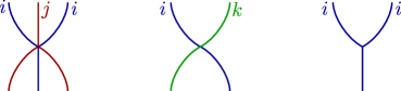
Figure 1. The types of vertices allowed in weaves. Here, we take $i,j$ and $k$ such that $i$ and $j$ are adjacent in $\mathsf{D}$, but $i$ and $k$ are not.

Each (generic) horizontal slice of a weave is a positive braid word, and we interpret weaves as sequences of braid words or “movies” of braids. By [14, Lemma 4.5], the Demazure products of all these braid words remain constant. In particular, if we start from a braid word $\beta$ on the top and the braid word at the bottom is reduced, then we get $\delta(\beta)$ on the bottom. This is expressed with the notation $\mathfrak{W}:\beta\to\delta(\beta)$. By convention, all our weaves will be oriented downwards.

Each slice of an algebraic weave carries a variable, with the variables on top being $z_{1},\dots,z_{r}$; this is capturing the variables in Corollary 3.7. The vertices correspond to the following equations between elements $B_{i}(z)$:

(9) $$B_{i}(z_{1})B_{j}(z_{2})B_{i}(z_{3})=B_{j}(z_{3})B_{i}(z_{1}z_{3}-z_{2})B_{j}(z_{1}),\ \quad B_{i}(z_{1})B_{k}(z_{2})=B_{k}(z_{2})B_{i}(z_{1})$$

(10) $$B_{i}(z_{1})B_{i}(z_{2})=B_{i}(z_{1}-z_{2}^{-1})U,\ \quad U=\varphi_{i}\left(\begin{matrix}z_{2}&-1\\ 0&z_{2}^{-1}\end{matrix}\right)$$

The equation (10) is defined only when $z_{2}\neq 0$ and can be applied in the middle of a product of several braid matrices. In this case, we apply Corollary 3.9 to move the element $U\in\mathsf{B}$ to the right of all the elements $B_{k}(z)$ appearing to the right of $B_{i}(z_{2})$. This implies that at every trivalent vertex we must modify all the variables appearing to the right of this vertex. Finally, we require that all variables on the bottom of the weave are equal to $0$, cf. Equation (7).

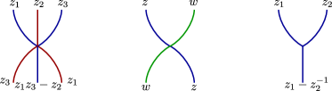
Figure 2. The effect that the basic weaves have on variables, which reflects Equations (9) and (10). Note that the rightmost weave is only defined when $z_{2}\neq 0$.

The results in [14] imply the following:

Lemma 4.1.

$($[14, Proposition 5.3,Corollary 5.5]$)$ Let $\beta\in\operatorname{Br}_{W}^{+}$ be a positive braid word and $\mathfrak{W}$ a Demazure weave. Then $\mathfrak{W}$ defines an open affine subset $T_{\mathfrak{W}}\subseteq X(\beta)$, isomorphic to the algebraic torus $(\mathbb{C}^{*})^{d}$, where $d$ is the number of trivalent vertices. In addition, the variables on all edges of $\mathfrak{W}$ are rational functions in the initial variables $z_{i}$, and (Laurent) coordinates on $T_{\mathfrak{W}}$ are given by the variables on the right incoming edges at trivalent vertices.

The following lemma is a more precise coordinate version of Remark 3.3:

Lemma 4.2.

Let $U_{0}\in\mathsf{B}$ and consider $X_{U_{0}}(\beta):=\{(z_{1},\dots,z_{r})\in\mathbb{C}^{r}\mid\delta^{-1}U_{0}B_{\beta}(z)\in\mathsf{B}\}$. Then there is a canonical isomorphism of varieties

$$\Phi:X(\beta)\xrightarrow{\sim}X_{U_{0}}(\beta).$$

Furthermore, given any weave for $\beta$, the isomorphism $\Phi$ extends uniquely to all variables in the weave, and for any slice $\gamma$ of the weave we have

$$U_{0}B_{\gamma}(\Phi(z))=B_{\gamma}(z)U.$$

Finally, the right incoming edge at every trivalent vertex is multiplied by a scalar depending only on the projection of $U_{0}$ to $T$.

Proof.

The existence and uniqueness of $\Phi$ follows from Corollary 3.9. To prove that $\Phi$ extends to a weave correctly, it is sufficient to check it for any vertex, and this is verified in [14, Section 5.2.1]. The last assertion follows from the identity (compare with [14, Section 5.2.1]):

$$\left(\begin{matrix}a&b\\ 0&c\end{matrix}\right)\left(\begin{matrix}z_{1}&-1\\ 1&0\end{matrix}\right)\left(\begin{matrix}z_{2}&-1\\ 1&0\\ \end{matrix}\right)=\left(\begin{matrix}\frac{z_{1}a+b}{c}&-1\\ 1&0\\ \end{matrix}\right)\left(\begin{matrix}\frac{c}{a}z_{2}&-1\\ 1&0\end{matrix}\right)\left(\begin{matrix}a&0\\ 0&c\end{matrix}\right).\qed$$

Remark 4.3.

The second part of Lemma 4.2 can be interpreted as an analogue of Lemma 4.1 for $X_{U_{0}}(\beta)$. Note, however, that we do not require that the variables $\Phi(z)$ at the bottom vanish, rather that $\Phi$ determines specific values for them $($which depend on the flag $U_{0}^{-1}\delta\mathsf{B}/\mathsf{B})$. In this sense, the second part of the Lemma 4.2 states that the isomorphism $\Phi$ preserves the torus $T_{\mathfrak{W}}$.

Following [18, Section 5], the torus $T_{\mathfrak{W}}$ has the following moduli interpretation, used repeatedly throughout the manuscript. The weave $\mathfrak{W}\subset\mathbb{R}^{2}$ is considered inside a rectangle $R\subset\mathbb{R}^{2}$ in such a way that $\mathfrak{W}\cap\partial R$ only has points in the northern and southern edges of $\partial R$. The northern edge intersection points dictate $\beta$ left-to-right, and the southern edge intersection points dictate $\delta(\beta)$ left-to-right. Then the weave itself $\mathfrak{W}$ describes an incidence problem in the flag variety $\mathsf{G}/\mathsf{B}$ as follows. For each connected component $C$ of $R\setminus\mathfrak{W}$, assign a flag $\mathsf{B}_{C}\in\mathsf{G}/\mathsf{B}$ such that:

1. $\mathsf{B}_{C_{-}}=\mathsf{B}$ for the unique connected component $C_{-}$ of $R\setminus\mathfrak{W}$ intersecting the left boundary of $R$.

2. $\mathsf{B}_{C_{+}}=\delta\mathsf{B}$ for the unique component $C_{+}$ of $R\setminus\mathfrak{W}$ intersecting the right boundary of $R$.

3. If $C,D\subset R\setminus\mathfrak{W}$ are separated by an edge of $\mathfrak{W}$ of color $i$, then we require $\mathsf{B}_{C}\buildrel s_{i}\over{\longrightarrow}\mathsf{B}_{D}$.

See Figure 3 for a depiction. Indeed, equations (9) and (10) imply that all flags $\mathsf{B}_{C}$ are determined by those flags corresponding to components intersecting the northern boundary of $R$. (In the setting of Lemma 4.2 the condition (2) should be replaced by $\mathsf{B}_{C_{+}}=U_{0}^{-1}\delta\mathsf{B}$, cf. Remark 4.3.)

Figure 3. A weave $\mathfrak{W}:\beta\to\delta(\beta)$ with its configuration of flags. Note that the flags $\mathsf{B}_{8},\dots,\mathsf{B}_{19}$ are completely determined by $(\mathsf{B},\mathsf{B}_{1},\dots,\mathsf{B}_{7},\mathsf{B}_{-})\in X(\beta)$, and that the flags $\mathsf{B}_{18}$ and $\mathsf{B}_{19}$ are coordinate flags.

4.2. Weave equivalence and mutations

The notion of weave mutation was introduced in [18, Section 4.8]. Equivalences between weaves, also known as moves, were discussed in [18, Theorem 1.1]. See also [14, Section 4]. The equivalence relation on weaves can be defined as follows:

• Let $\mathfrak{W},\mathfrak{W}^{\prime}:\beta\to\beta^{\prime}$ consist only of braid moves, i.e. 4- and 6- valent vertices, where $\beta,\beta^{\prime}$ are two positive braids words representing the same element in the braid group $\operatorname{Br}^{+}_{W}$. Then $\mathfrak{W}$ and $\mathfrak{W}^{\prime}$ are equivalent.

• Suppose that $i,j\in\mathsf{D}$ are adjacent. Then the weaves $ijij\to jijj\to jij$ and $ijij\to iiji\to iji\to jij$ are equivalent. See Figure 4.

• Suppose that $i,j\in\mathsf{D}$ are not adjacent. Then the weaves $iji\to iij\to ij\to ji$ and $iji\to jii\to ji$ are equivalent. In other words, one can move a $j$-colored strand through an $i$-colored trivalent vertex.

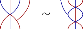
Figure 4. The two equivalent weaves in $(ii)$: the two weaves $ijij\to jijj\to jij$, depicted on the left, and $ijij\to iiji\to iji\to jij$, on the right, are declared equivalent.

The relations (ii) and (iii) are parameterized by rank $2$ subdiagrams of $\mathsf{D}$ which are of types $A_{2}$ and $A_{1}\times A_{1}$ respectively. To ease notation, we often write $i=1$ and $j=2$ for the second case, so that we have an $A_{2}$ subdiagram of $\mathsf{D}$; we therefore refer to the braid word $ijij$ on top of Figure 4 as 1212. Note that the weave calculus in [14, 18] used two more equivalence relations. The first relation was that all weaves from 12121 to 121 are equivalent – by [14, Section 4.2.5] this is a consequence of our equivalence relation (ii) for 1212. The second relation was the Zamolodchikov relation for different paths of reduced expressions for the longest element in $A_{3}$. Such reduced expressions are related by a sequence of braid moves, and hence any two weaves of this type are equivalent by item (i). In the same vein, applying the same braid relation twice $121\to 212\to 121$ is equivalent to doing nothing. Finally, [14, Section 5] shows that two equivalent weaves $\mathfrak{W}_{1}$ and $\mathfrak{W}_{2}$ yield equal tori, i.e. $T_{\mathfrak{W}_{1}}=T_{\mathfrak{W}_{2}}$.

The two weaves for $iii\to i$ depicted in Figure 5 are not equivalent. By definition, these two weaves are said to be are related by weave mutation. Two weaves $\mathfrak{W}_{1},\mathfrak{W}_{2}$ that differ by a weave mutation do not yield equal tori, i.e. $T_{\mathfrak{W}_{1}}\neq T_{\mathfrak{W}_{2}}$.

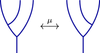
Figure 5. Weave mutation

Lemma 4.4.

Let $\mathfrak{W}_{1},\mathfrak{W}_{2}:\beta\to\delta(\beta)$ be Demazure weaves, where we have fixed a braid word for $\delta(\beta)$. Then $\mathfrak{W}_{1}$ and $\mathfrak{W}_{2}$ are related by a sequence of equivalence moves and mutations.

Proof.

In type $A$ this is proved in [14, Theorem 4.6]. For arbitrary simply laced type, we consider all possible positions in a braid word where one can apply the operations $ii\to i$ and braid relations. If such positions do not overlap, the operations commute. If they overlap, then these involve at most 3 different simple reflections, hence the problem is reduced to a rank 3 subgroup of $W$. Since any rank 3 subgroup is of type $A$, the result follows. A direct proof can also be provided by arguing as in [14, Theorem 4.11]. ∎

4.3. Inductive weaves

Both [18] and [14, Section 4] provide construction for weaves. In this subsection, we introduce two distinguished Demazure weaves $\overrightarrow{\mathfrak{w}}(\beta),\overleftarrow{\mathfrak{w}}(\beta):\beta\to\delta(\beta)$ that will yield the initial cluster seeds in our proofs.

Definition 4.5.

The left inductive weave $\overleftarrow{\mathfrak{w}}(\beta):\beta\to\delta(\beta)$ is the weave constructed as follows:

• $\overleftarrow{\mathfrak{w}}(\beta)$ is the empty weave if $\beta$ is the empty word.

• Suppose that $\delta(\sigma_{i}\beta)=s_{i}\delta(\beta)$. Then $\overleftarrow{\mathfrak{w}}(\sigma_{i}\beta)$ is obtained as the concatenation of $\overleftarrow{\mathfrak{w}}(\beta)$ and a vertical $s_{i}$-strand to its left.

• Suppose that $\delta(\sigma_{i}\beta)=\delta(\beta)$. Then, choose a braid word for $\delta(\beta)$ which starts at $s_{i}$ and form $\overleftarrow{\mathfrak{w}}(\sigma_{i}\beta)$ by appending a trivalent vertex labeled by $s_{i}$ to the bottom left of $\overleftarrow{\mathfrak{w}}(\beta)$.

The right inductive weave $\overrightarrow{\mathfrak{w}}(\beta)$ is defined analogously, instead reading the braid word $\beta$ left-to-right and having all the trivalent vertices to its right.

There are choices in defining the left or right inductive weave, and the weave depends on these choices. Nevertheless, all these inductive weaves are equivalent. Note also that, while the variety $X(\beta)$ does not depend on the choice of a word for $\beta$, both of the weaves $\overleftarrow{\mathfrak{w}}(\beta)$ and $\overrightarrow{\mathfrak{w}}(\beta)$ do depend on the word. We elaborate on this in Section 4.9.

Remark 4.6.

By construction, a weave $\mathfrak{W}:\beta\to\delta(\beta)$ is left $($resp. right$)$ inductive if and only if the left $($resp. right$)$ edge of each trivalent vertex $v$ goes all the way to the top. Thus, trivalent vertices in such weaves can be identified with certain letters in $\beta$. The trivalent vertices in a left $($resp. right$)$ inductive weave are parameterized by the letters in the complement of the rightmost $($resp. leftmost$)$ reduced subword for $\delta(\beta)$ inside the word for $\beta$.

Both left and right inductive weaves are special cases of double inductive weaves defined below in Section 6.4.

4.4. Lusztig cycles

Following the geometry of 1-cycles on surfaces represented by weaves, as developed in [18, Section 2], we now present the algebraic notion of a cycle on a weave $\mathfrak{W}$ that works for any $\mathsf{G}$.

Definition 4.7.

A cycle in $\mathfrak{W}$ is a function $C:E(\mathfrak{W})\to\mathbb{Z}_{\geq 0}$ that assigns a non-negative integer to each edge of the weave. The values of $C$ are referred to as the weights of the edges in $C$.

If two weaves $\mathfrak{W}_{1},\mathfrak{W}_{2}$ can be vertically concatenated (i.e. the southern boundary of $\mathfrak{W}_{1}$ coincides with the northern boundary of $\mathfrak{W}_{2}$) and $C_{i}$ is a cycle on $\mathfrak{W}_{i}$, then the cycles $C_{i}$ can be concatenated provided that their values agree on the southern edges of $\mathfrak{W_{1}}$, which are the northern edges of $\mathfrak{W}_{2}$. We denote the concatenation of the cycles by $C_{2}\circ C_{1}:E(\mathfrak{W}_{2}\circ\mathfrak{W}_{1})\to\mathbb{Z}_{\geq 0}$.

Given a weave $\mathfrak{W}:\beta\to\delta(\beta)$, we will extract a quiver from a particular collection of cycles and an intersection form defined on that collection. Let us focus on constructing such a collection, motivated by work of G. Lusztig on total positivity [56]. For that, let $x_{i}(t)=\exp(E_{i}t)$ be the one-parameter subgroup in $\mathsf{G}$ corresponding to the positive simple root $\alpha_{i}$; in particular, $x_{i}(t_{1})x_{i}(t_{2})=x_{i}(t_{1}+t_{2})$. In addition, if $i,j\in\mathsf{D}$ are not adjacent, then

$$x_{i}(t_{1})x_{j}(t_{2})=x_{j}(t_{2})x_{i}(t_{1}).$$

If $i,j\in\mathsf{D}$ are adjacent, and $t_{1}+t_{3}\neq 0$, then

$$x_{i}(t_{1})x_{j}(t_{2})x_{i}(t_{3})=x_{j}\left(\frac{t_{2}t_{3}}{t_{1}+t_{3}}\right)x_{i}(t_{1}+t_{3})x_{j}\left(\frac{t_{1}t_{2}}{t_{1}+t_{3}}\right).$$

These can be verified directly [56, Proposition 2.5]. These relations can be considered as rational maps

(11) $$\varphi_{1}:(t_{1},t_{2})\mapsto t_{1}+t_{2},\quad\varphi_{2}:(t_{1},t_{2})\mapsto(t_{2},t_{1}),\ \quad\varphi_{3}:(t_{1},t_{2},t_{3})\mapsto\left(\frac{t_{2}t_{3}}{t_{1}+t_{3}},t_{1}+t_{3},\frac{t_{1}t_{2}}{t_{1}+t_{3}}\right).$$

The coordinates $(t_{i})_{i\in\mathsf{D}}$ are referred to as Lusztig’s coordinates for $\mathsf{G}$ in [24, Section 1.2.6] and as Lusztig factorization coordinates in [68, Definition 3.12]. A tropical version of the maps $\varphi_{1},\varphi_{2},\varphi_{3}$ is obtained by replacing multiplication with addition and addition with $\min$. The rational maps $\varphi_{1},\varphi_{2},\varphi_{3}$ then become

(12) $$\Phi_{1}:(a_{1},a_{2})\mapsto\min(a_{1},a_{2}),\quad\Phi_{2}:(a_{1},a_{2})\mapsto(a_{2},a_{1}),\\ \Phi_{3}:(a_{1},a_{2},a_{3})\mapsto\left(a_{2}+a_{3}-\min(a_{1},a_{3}),\min(a_{1},a_{3}),a_{1}+a_{2}-\min(a_{1},a_{3})\right).\hskip 79.6678pt$$

Note that the equations for $\Phi_{1},\Phi_{2}$ and $\Phi_{3}$ do not depend on the indices $i,j$ of the corresponding simple roots, and $\Phi_{3}^{2}(a_{1},a_{2},a_{3})=(a_{1},a_{2},a_{3})$. These tropicalization maps define the following collection of cycles on a Demazure weave.

Definition 4.8.

Let $\mathfrak{W}$ be a Demazure weave. A Lusztig cycle is a cycle $C:E(\mathfrak{W})\to\mathbb{Z}_{\geq 0}$ satisfying the following conditions.

• For a trivalent vertex with incoming edges $e_{1},e_{2}$ and outgoing edge $e$, $C$ satisfies

  $$C(e)=\Phi_{1}(C(e_{1}),C(e_{2}))$$

• For a 4-valent vertex with incoming edges $e_{1},e_{2}$ and outgoing edges $e_{1}^{\prime},e_{2}^{\prime}$, $C$ satisfies

  $$(C(e^{\prime}_{1}),C(e^{\prime}_{2}))=\Phi_{2}(C(e_{1}),C(e_{2}))$$

• For a 6-valent vertex with incoming edges $e_{1},e_{2},e_{3}$ and outgoing edges $e_{1}^{\prime},e_{2}^{\prime},e^{\prime}_{3}$, $C$ satisfies

  $$(C(e^{\prime}_{1}),C(e^{\prime}_{2}),C(e^{\prime}_{3}))=\Phi_{3}(C(e_{1}),C(e_{2}),C(e_{3}))$$

Definition 4.8 implies that the weights of a Lusztig cycle on a weave are completely determined by the weights of the top edges. In fact, the following strengthening holds.

Lemma 4.9.

Let $\mathfrak{W}:\beta\to u$ be a Demazure weave, where $u=\delta(\beta)$ is a choice of reduced braid word, and $C$ a Lusztig cycle. Then, given the input values of $C$ on $\beta$, the output values on $u$ do not depend on the weave $\mathfrak{W}$.

Proof.

Suppose that $\beta=\sigma_{i_{1}}\cdots\sigma_{i_{\ell}}$ and $u=\sigma_{j_{1}}\cdots\sigma_{j_{k}}$, and choose variables $t_{1},\ldots,t_{\ell},t^{\prime}_{1},\ldots,t^{\prime}_{k}\in\mathbb{C}$. Consider the factorization problem

$$x_{\beta}(t)=x_{i_{1}}(t_{1})\cdots x_{i_{\ell}}(t_{\ell})=x_{j_{1}}(t^{\prime}_{1})\cdots x_{j_{k}}(t^{\prime}_{k})=x_{u}(t^{\prime}).$$

For a fixed weave, Equation (11) implies that the variables $t^{\prime}_{j}$ can be written as certain rational functions in $t_{1},\ldots,t_{\ell}$, where both numerator and denominator have nonnegative coefficients. Indeed, apply $\varphi_{1},\varphi_{2},\varphi_{3}$ at every 3-,4- and 6-valent vertex, respectively. By [29, Proposition 2.18], see also [56], the map

$$(t^{\prime}_{1},\ldots,t^{\prime}_{k})\mapsto x_{u}(t^{\prime})=x_{j_{1}}(t^{\prime}_{1})\ldots x_{j_{k}}(t^{\prime}_{k})$$

is an isomorphism between $(\mathbb{C}^{*})^{k}$ and a Zariski open subset of a Schubert cell. In particular, $t^{\prime}_{1},\ldots,t^{\prime}_{k}$ are uniquely determined by $x_{u}(t^{\prime})$ and hence by $t_{1},\ldots,t_{\ell}$. Then the lemma follows by tropicalization of the above argument. ∎

The following identity will be useful.

Lemma 4.10.

Let $a,b,c,d\in\mathbb{Z}$, then

$$\min\left(a,c+d-\min(b,d)\right)+\min(b,d)=\min\left(d,a+b-\min(a,c)\right)+\min(a,c).$$

Proof.

This is a tropicalization of the following identity, which is readily verified by direct computation:

$$\left(t^{a}+\frac{t^{c}t^{d}}{t^{b}+t^{d}}\right)(t^{b}+t^{d})=\left(t^{d}+\frac{t^{a}t^{b}}{t^{a}+t^{c}}\right)(t^{a}+t^{c}).\qed$$

Example 4.11.

Consider the pair of Demazure weaves $\mathfrak{W}_{1},\mathfrak{W}_{2}$ for the braid word $\beta=1212$ as in Figure 4, where $\mathfrak{W}_{1}$ is the left figure and $\mathfrak{W}_{2}$ is the right figure. Suppose that the incoming edges for a cycle have weights $a,b,c,d$. Then $\mathfrak{W}_{1}$ has the form $1212\to 2122\to 212$ and the weights transform as follows:

$$(a,b,c,d)\mapsto\left(b+c-\min(a,c),\min(a,c),a+b-\min(a,c),d\right)\mapsto\\ \left(b+c-\min(a,c),\min(a,c),\min(a+b-\min(a,c),d)\right)=:(a^{\prime},b^{\prime},c^{\prime}).$$

The weave $\mathfrak{W}_{2}$ has the form $1212\to 1121\to 121\to 212$ and the weights transform as:

$$(a,b,c,d)\to(a,c+d-\min(b,d),\min(b,d),b+c-\min(b,d))\to\\ (\min(a,c+d-\min(b,d)),\min(b,d),b+c-\min(b,d))\to(a^{\prime\prime},b^{\prime\prime},c^{\prime\prime}),$$

where we have that

$$b^{\prime\prime}=\min(\min(a,c+d-\min(b,d)),b+c-\min(b,d))=\min(a,c+d-\min(b,d),b+c-\min(b,d))=$$

$$\min(a,\min(b,d)+c-\min(b,d))=\min(a,c).$$

By Lemma 4.10, the weights also satisfy $a^{\prime\prime}=b+c-b^{\prime\prime}=b+c-\min(a,c)$ and

$$c^{\prime\prime}=\min(a,c+d-\min(b,d))+\min(b,d)-b^{\prime\prime}=c^{\prime}.$$

The cycles that lead to an initial quiver are associated to trivalent vertices of a weave. These cycles are not directly Lusztig cycles, but are “Lusztig cycles below the trivalent vertex $v$”, in the following sense.

Definition 4.12.

Let $\mathfrak{W}$ be a Demazure weave and $v\in\mathfrak{W}$ be a trivalent vertex. Given the decomposition $\mathfrak{W}=\mathfrak{W}_{2}\circ\mathfrak{W}_{1}$, where the southernmost edge of $\mathfrak{W}_{1}$ is the outgoing edge of the trivalent vertex $v$, the cycle $\gamma_{v}$ is defined to be the concatenation $\gamma_{v}:=C_{2}\circ C_{1}$, where

• $C_{1}:E(\mathfrak{W}_{1})\to\mathbb{Z}_{\geq 0}$ is the cycle that assigns weight $0$ that all edges except for the (downwards) outgoing edge of the trivalent vertex $v$, to which $C_{1}$ assigns weight $1$.

• $C_{2}:E(\mathfrak{W}_{2})\to\mathbb{Z}_{\geq 0}$ is the unique Lusztig cycle that can be concatenated with $C_{1}$.

The cycles $\gamma_{v}$ in Definition 4.12, $v\in\mathfrak{W}$ a trivalent vertex, will often be referred to as Lusztig cycles as well, in a minor abuse of notation and only when the context is clear, given that they are Lusztig cycles except at their origin vertex $v$. The following terminology is also useful.

Definition 4.13.

Let $\mathfrak{W}$ be a Demazure weave and $v\in\mathfrak{W}$ be a trivalent vertex. By definition, $\gamma_{v}$ is said to bifurcate at a $6$-valent vertex with incoming edges $e_{1},e_{2},e_{3}$ and outgoing edges $e_{1}^{\prime},e_{2}^{\prime},e^{\prime}_{3}$ if

$$\gamma_{v}(e_{1})=\gamma_{v}(e_{3})=0,\gamma_{v}(e_{2})\neq 0.$$

Note that this implies that $\gamma_{v}(e^{\prime}_{1}),\gamma_{v}(e^{\prime}_{3})\neq 0$ and $\gamma_{v}(e^{\prime}_{2})=0$, justifying the terminology. By definition, $\gamma_{v}$ is non-bifurcating if it never bifurcates.

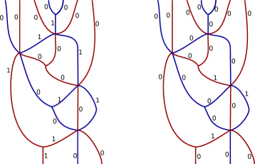
Figure 6. The cycles $\gamma_{v}$ associated to the topmost trivalent vertex (left) and second topmost trivalent vertices (right) of the weave.

Example 4.14.

Consider the weave $\mathfrak{W}:\beta=\sigma_{1}\sigma_{2}\sigma_{2}\sigma_{1}\sigma_{1}\sigma_{2}\sigma_{2}\to\sigma_{2}\sigma_{1}\sigma_{2}$ in Figure 6. The cycles $\gamma_{v}$ for the topmost (resp. second topmost) trivalent vertices are also depicted in Figure 6 left (resp. right). The cycle on the left bifurcates at two $6$-valent vertices, while the cycle on the right is non-bifurcating.

Remark 4.15.

Note that relations similar to those in Definition 4.8 appear in the definition of Mirković-Vilonen polytopes [50, Proposition 5.2]. The connection between the cycles on Demazure weaves and Mirković-Vilonen polytopes is intriguing and we plan to investigate it in the future.

4.5. Local intersections

In our construction, the arrows of the quiver $Q_{\mathfrak{W}}$, which we discuss momentarily, are determined by considering (local) intersection numbers between cycles on $\mathfrak{W}$. Given two cycles $C,C^{\prime}:E(\mathfrak{W})\to\mathbb{Z}_{\geq 0}$ on a weave $\mathfrak{W}$, we now define their intersection number as a sum of local contributions from intersections at the 3-valent and 6-valent vertices and a boundary intersection term.

Definition 4.16 (Local intersection at 3-valent vertex).

Let $\mathfrak{W}$ be a Demazure weave, $v\in\mathfrak{W}$ a trivalent vertex, and $C,C^{\prime}:E(\mathfrak{W})\to\mathbb{Z}_{\geq 0}$ two cycles. Suppose that $C$ $($resp.  $C^{\prime})$ has weights $a_{1},a_{2}$ $($resp. $b_{1},b_{2})$ on the incoming edges of a trivalent vertex $v$, and the weight $a^{\prime}$ $($resp. $b^{\prime})$ on the outgoing edge. By definition, the local intersection number of $C,C^{\prime}$ at $v$ is

$$\sharp_{v}(C\cdot C^{\prime})=\left|\begin{matrix}1&1&1\\ a_{1}&a^{\prime}&a_{2}\\ b_{1}&b^{\prime}&b_{2}\\ \end{matrix}\right|.$$

Definition 4.17 (Local intersection at 6-valent vertex).

Let $\mathfrak{W}$ be a Demazure weave, $v\in\mathfrak{W}$ a hexavalent vertex, and $C,C^{\prime}:E(\mathfrak{W})\to\mathbb{Z}_{\geq 0}$ two cycles. Suppose that $C$ $($resp. $C^{\prime})$ has weights $a_{1},a_{2},a_{3}$ $($resp. $b_{1},b_{2},b_{3})$ on the incoming edges of a 6-valent vertex $v$, and weights $a^{\prime}_{1},a^{\prime}_{2},a^{\prime}_{3}$ $($resp. $b^{\prime}_{1},b^{\prime}_{2},b^{\prime}_{3})$ on the outgoing edges. By definition, the local intersection number of $C,C^{\prime}$ at $v$ is

$$\sharp_{v}(C\cdot C^{\prime})=\frac{1}{2}\left(\left|\begin{matrix}1&1&1\\ a_{1}&a_{2}&a_{3}\\ b_{1}&b_{2}&b_{3}\\ \end{matrix}\right|-\left|\begin{matrix}1&1&1\\ a^{\prime}_{1}&a^{\prime}_{2}&a^{\prime}_{3}\\ b^{\prime}_{1}&b^{\prime}_{2}&b^{\prime}_{3}\\ \end{matrix}\right|\right).$$

Example 4.18.

Let $C,C^{\prime}$ be Lusztig cycles. Suppose $C$ has weights $(a_{1},a_{2},a_{3})=(1,0,0)$ on the top of $v$. Therefore $(a^{\prime}_{1},a^{\prime}_{2},a^{\prime}_{3})=(0,0,1)$. Then their local intersection at $v$ is

$$\sharp_{v}(C\cdot C^{\prime})=\frac{1}{2}\left(b_{2}-b_{3})-(b^{\prime}_{1}-b^{\prime}_{2})\right).$$

Since $b^{\prime}_{1}=b_{2}+b_{3}-b^{\prime}_{2}$, we get $\sharp_{v}(C\cdot C^{\prime})=b^{\prime}_{2}-b_{3}$, and $\sharp_{v}(C^{\prime}\cdot C)=b_{3}-b^{\prime}_{2}.$

Lemma 4.19.

Let $\mathfrak{W}$ be a weave and $v$ a 6-valent vertex $v$. Consider three Lusztig cycles $C,C^{\prime},C^{\prime\prime}$ whose weights are $(a_{1},a_{2},a_{3})$, $(b_{1},b_{2},b_{3})$ and $(c_{1},c_{2},c_{3})$ on the top of $v$. Then the following holds:

• If $(c_{1},c_{2},c_{3})=(b_{1},b_{2},b_{3})+(1,0,1)$ then $\sharp_{v}(C\cdot C^{\prime})=\sharp_{v}(C\cdot C^{\prime\prime})$.

• If $(c_{1},c_{2},c_{3})=(b_{1},b_{2},b_{3})+(0,1,0)$ then $\sharp_{v}(C\cdot C^{\prime})=\sharp_{v}(C\cdot C^{\prime\prime})$.

Proof.

For $(1)$, we have $\min(c_{1},c_{3})=\min(b_{1},b_{3})+1$ and $(c^{\prime}_{1},c^{\prime}_{2},c^{\prime}_{3})=(b^{\prime}_{1},b^{\prime}_{2},b^{\prime}_{3})+(0,1,0)$. The local intersection number being bilinear, it suffices to consider $(b_{1},b_{2},b_{3})=(0,0,0)$. Then $\sharp(C\cdot C^{\prime})=0$ equals

$$\sharp(C\cdot C^{\prime\prime})=\frac{1}{2}\left(\left|\begin{matrix}1&1&1\\ a_{1}&a_{2}&a_{3}\\ 1&0&1\\ \end{matrix}\right|-\left|\begin{matrix}1&1&1\\ a^{\prime}_{1}&a^{\prime}_{2}&a^{\prime}_{3}\\ 0&1&0\\ \end{matrix}\right|\right)=\frac{1}{2}\left((a_{3}-a_{1})-(a^{\prime}_{1}-a^{\prime}_{3})\right)=0,$$

as required. The proof of $(2)$ is similar. ∎

Definition 4.20.

Let $\mathfrak{W}$ be a weave and $C,C^{\prime}:E(\mathfrak{W})\to\mathbb{Z}_{\geq 0}$ cycles. By definition, the intersection number $\sharp_{\mathfrak{W}}(C\cdot C^{\prime})$ of $C$ and $C^{\prime}$ is

$$\sharp_{\mathfrak{W}}(C\cdot C^{\prime}):=\sum_{v\,3\text{-valent}}\sharp_{v}(C\cdot C^{\prime})+\sum_{v\,6\text{-valent}}\sharp_{v}(C\cdot C^{\prime})$$

Note that $\sharp_{\mathfrak{W}}(C\cdot C^{\prime})=-\sharp_{\mathfrak{W}}(C^{\prime}\cdot C)$ and that $\sharp_{\mathfrak{W}}(C\cdot C^{\prime})$ is an integer when $C,C^{\prime}$ are both Lusztig cycles.

4.6. Quiver from local intersections

Let $\mathfrak{W}$ be a Demazure weave. Definition 4.20, along with the following notion of boundary intersections in Definition 4.21, allow us to associate a quiver $Q_{\mathfrak{W}}$ to $\mathfrak{W}$.

Recall the Cartan subgroup $T$. Denote by $X$ and $X^{\vee}$ the lattices of characters and cocharacters of $T$. Consider the perfect pairing

(13) $$(\cdot,\cdot):~{}X\times X^{\vee}\longrightarrow\mathbb{Z}.$$

Let $\{\alpha_{i}\}$ and $\{\alpha_{i}^{\vee}\}$ be the set of simple roots and simple coroots, indexed by the vertices in $\mathsf{D}$. Now given a braid word $\beta=\sigma_{i_{1}}\cdots\sigma_{i_{k}}$, we consider the following sequences of roots and coroots (cf. [19]):

(14) $$\rho_{j}:=s_{i_{1}}\cdots s_{i_{j-1}}(\alpha_{i_{j}}),\qquad\rho_{j}^{\vee}:=s_{i_{1}}\cdots s_{i_{j-1}}(\alpha_{i_{j}}^{\vee}),\qquad\forall 1\leq j\leq k.$$

Note that $\rho_{j}=s_{i_{1}}\cdots s_{i_{j}}(-\alpha_{i_{j}})$. For a weave $\mathfrak{W}$ and a cycle $C$, such that $\beta$ appears as a horizontal section of $\mathfrak{W}$, we denote by $c_{j}$ the weight of $C$ on the $j$-th letter of $\beta$.

Definition 4.21.

Let $\mathfrak{W}$ be a weave and $C,C^{\prime}:E(\mathfrak{W})\to\mathbb{Z}_{\geq 0}$ cycles and $\beta=\sigma_{i_{1}}\cdots\sigma_{i_{r}}$ a braid word which is a horizontal section of $\mathfrak{W}$. By definition, the boundary intersection $\sharp_{\beta}(C\cdot C^{\prime})$ of $C,C^{\prime}$ at $\beta$ is

$$\sharp_{\beta}(C\cdot C^{\prime}):=\frac{1}{2}\sum_{i,j=1}^{r}\operatorname{sign}(j-i)c_{i}c^{\prime}_{j}\cdot(\rho_{i},\rho_{j}^{\vee})$$

where $(\cdot,\cdot)$ is the pairing defined via (13), and

$$\operatorname{sign}(k)=\begin{cases}1&\mbox{if }k>0,\\ 0&\mbox{if }k=0,\\ -1&\mbox{if }k<0.\end{cases}$$

Remark 4.22.

In Definition 4.21 and throughout this section we are assuming that the group $\mathsf{G}$ is of simply laced type. For non-simply laced type Definition 4.21 has to be modified to take into account cycles for the Langlands dual group $\mathsf{G}^{\vee}$ of $\mathsf{G}$, see Section 6.1 and in particular (27) below.

Definition 4.23.

Let $\mathfrak{W}$ be a Demazure weave. By definition, the quiver $Q_{\mathfrak{W}}$ is the quiver whose vertices are (in bijective correspondence with) the trivalent vertices of $\mathfrak{W}$, and whose adjacency matrix is given by

$$\varepsilon_{v,v^{\prime}}:=\sharp_{\mathfrak{W}}(\gamma_{v}\cdot\gamma_{v^{\prime}})+\sharp_{\delta(\beta)}(\gamma_{v}\cdot\gamma_{v^{\prime}}).$$

where $\delta(\beta)$ is the bottom slice of the weave $\mathfrak{W}$.

Remark 4.24.

The entries $\varepsilon_{v,v^{\prime}}$ in Definition 4.23 are always half-integers but not necessarily integers. Note also that the boundary intersection terms for $\varepsilon_{v,v^{\prime}}$ vanish for cycles $\gamma_{v},\gamma_{v^{\prime}}$ (either of) which do not reach the bottom part of the weave: in the language of Subsection 4.7, the boundary intersection terms only appear between frozen vertices, and the weights of arrows between mutable vertices are always integers.

Let us now continue our study of $Q_{\mathfrak{W}}$ and its dependence on the weave $\mathfrak{W}$.

Lemma 4.25.

Let $\mathfrak{W}$ be a weave with no trivalent vertices. Then for any two Lusztig cycles $C,C^{\prime}$ the sum of local intersection numbers equals the difference of boundary intersection numbers.

Proof.

It suffices to verify this for a single 6-valent vertex and a single $4$-valent vertex, which are local computations. For the former, suppose that the Lusztig cycle $C$ has weights $(a_{1},a_{2},a_{3})$ on top of a $6$-valent vertex, while the Lusztig cycle $C^{\prime}$ has weights $(b_{1},b_{2},b_{3})$, also on top. By Lemma 4.19, we can assume that $a_{2}=a_{3}=b_{2}=b_{1}=0$, so the intersection number around the $6$-valent vertex is $\sharp(C\cdot C^{\prime})=-a_{1}b_{3}$. We may also assume that the roots at the top boundary are $\rho_{3}=\alpha_{j}$, $\rho_{2}=\alpha_{i}+\alpha_{j}$ and $\rho_{1}=\alpha_{i}$ where $i,j\in\mathsf{D}$ are adjacent. Thus, the top intersection number is

$$\#_{\mathrm{top}}(C\cdot C^{\prime})=\frac{1}{2}\operatorname{sign}(3-1)a_{1}b_{3}(\alpha_{i},\alpha_{j}^{\vee})=-\frac{1}{2}a_{1}b_{3}$$

and the bottom intersection number is

$$\#_{\mathrm{bottom}}(C\cdot C^{\prime})=\frac{1}{2}\operatorname{sign}(1-3)a^{\prime}_{3}b^{\prime}_{1}(\alpha_{j},\alpha_{i}^{\vee})=\frac{1}{2}a_{1}b_{3}$$

and the result for $6$-valent vertices follows. For a $4$-valent vertex, suppose that we have Lusztig cycles $C$, $C^{\prime}$ with weights $a_{1},a_{2}$ and $b_{1},b_{2}$ at the top, respectively. Then the top boundary intersection number is $a_{1}b_{2}-a_{2}b_{1}$, while the bottom boundary intersection number is $a^{\prime}_{1}b^{\prime}_{2}-a^{\prime}_{2}b^{\prime}_{1}=a_{2}b_{1}-a_{1}b_{2}$. Thus, the difference between the boundary intersection numbers is $0$, as required. ∎

Corollary 4.26.

Let $\mathfrak{W}_{1},\mathfrak{W}_{2}:\beta\to\beta^{\prime}$ be two weaves with no trivalent vertices. Suppose that $C_{\mathfrak{W}_{1}},C^{\prime}_{\mathfrak{W}_{1}}$ are Lusztig cycles in $\mathfrak{W}_{1}$, $C_{\mathfrak{W}_{2}},C^{\prime}_{\mathfrak{W}_{2}}$ are Lusztig cycles in $\mathfrak{W}_{2}$, and the initial weights of $C_{\mathfrak{W}_{1}}$ $($resp. $C^{\prime}_{\mathfrak{W}_{1}})$ are the same as those of $C_{\mathfrak{W}_{2}}$ $($resp. $C^{\prime}_{\mathfrak{W}_{2}})$. Then $\sharp_{\mathfrak{W}_{1}}(C\cdot C^{\prime})=\sharp_{\mathfrak{W}_{2}}(C\cdot C^{\prime}).$

Proof.

Indeed, both intersection numbers are equal to $\sharp_{\beta}(C\cdot C^{\prime})-\sharp_{\beta^{\prime}}(C\cdot C^{\prime}).$ Note that by Lemma 4.9 the output weights of $C_{\mathfrak{W}_{1}}$ $($resp. $C^{\prime}_{\mathfrak{W}_{1}})$ are the same as those of $C_{\mathfrak{W}_{2}}$ $($resp. $C^{\prime}_{\mathfrak{W}_{2}})$. ∎

Corollary 4.26 implies that two weaves $\mathfrak{W},\mathfrak{W}^{\prime}$ that are equivalent via an equivalence that uses only $4$- and $6$-valent vertices, then the corresponding quivers $Q_{\mathfrak{W}}$ and $Q_{\mathfrak{W}^{\prime}}$ coincide. Let us now prove the stronger result that any two equivalent weaves yield the same quiver. For that, it suffices to study weave equivalences that involve $3$-valent vertices, which locally are those in Example 4.11, see Figure 4.

Lemma 4.27.

Let $\mathfrak{W}_{1}:1212\to 2122\to 212$ and $\mathfrak{W}_{2}:1212\to 1121\to 121\to 212$ and $C_{i},C^{\prime}_{i}$ be Lusztig cycles on $\mathfrak{W}_{i}$, $i=1,2$. Suppose that the initial weights of $C_{1}$ $($resp. $C^{\prime}_{1})$ coincide with those of $C_{2}$ $($resp. $C^{\prime}_{2})$, and let $\gamma^{i}_{v}$ be the cycle originating at the unique trivalent vertex of $\mathfrak{W}_{i}$. Then we have the equalities:

• $\sharp_{\mathfrak{W}_{1}}(C_{1},\gamma^{1}_{v})=\sharp_{\mathfrak{W}_{2}}(C_{2},\gamma^{2}_{v})$

• $\sharp_{\mathfrak{W}_{1}}(C_{1},C^{\prime}_{1})=\sharp_{\mathfrak{W}_{2}}(C_{2},C^{\prime}_{2})$

Proof.

For (1), we follow the notations of Example 4.11, so $C_{1},C_{2}$ have weights $a,b,c,d$ on the top. For the weave $\mathfrak{W}_{1}$, the only local intersection is at trivalent vertex and thus

$$\sharp_{\mathfrak{W}_{1}}(C_{1},\gamma_{v}^{1})=a+b-\min(a,c)-d.$$

For $\mathfrak{W}_{1}$, the local intersection at trivalent vertex equals $a-c-d+\min(b,d)$, while the local intersection at the bottom 6-valent vertex equals $b+c-\min(b,d)-\min(a,c)$, as in Example 4.18. By combining these together we also obtain

$$\sharp_{\mathfrak{W}_{2}}(G,G_{v})=(a-c-d+\min(b,d))+(b+c-\min(b,d)-\min(a,c))=a+b-\min(a,c)-d.$$

For (2), Lemma 4.19, implies that adding $(1,0,1,0)$ and $(0,1,0,1)$ on top of either weave does not change the intersection number at any vertex of either weave. Thus we assume that $C_{i}$ and $C^{\prime}_{i}$ have weights $(a,0,0,b)$ and $(c,0,0,d)$ on top, where $a,b,c,d\in\mathbb{Z}$. Note that $a,b,c,d$ could be negative here. Denote $m_{ab}:=\min([a]_{+},b)$ and $m_{cd}:=\min([c]_{+},d)$ and let us compute the intersection numbers for $\mathfrak{W}_{1}$. At the 6-valent vertex we have

$$\frac{1}{2}\left|\begin{matrix}1&1&1\\ a&0&0\\ c&0&0\\ \end{matrix}\right|-\frac{1}{2}\left|\begin{matrix}1&1&1\\ -[a]_{-}&[a]_{-}&[a]_{+}\\ -[c]_{-}&[c]_{-}&[c]_{+}\\ \end{matrix}\right|=[a]_{+}[c]_{-}-[a]_{-}[c]_{+}.$$

At the 3-valent vertex we have

$$\left|\begin{matrix}1&1&1\\ [a]_{+}&m_{ab}&b\\ [c]_{+}&m_{cd}&d\\ \end{matrix}\right|=m_{ab}([d]_{+}+[d]_{-}-[c]_{+})+m_{cd}([a]_{+}-[b]_{+}-[b]_{-})+$$

$$[b]_{+}[c]_{+}+[b]_{-}[c]_{+}-[a]_{+}[d]_{+}-[a]_{+}[d]_{-}.$$

The intersection numbers for $\mathfrak{W}_{2}$ are as follows; at the top 6-valent vertex we have

$$\frac{1}{2}\left|\begin{matrix}1&1&1\\ 0&0&b\\ 0&0&d\\ \end{matrix}\right|-\frac{1}{2}\left|\begin{matrix}1&1&1\\ [b]_{+}&[b]_{-}&-[b]_{-}\\ [d]_{+}&[d]_{-}&-[d]_{-}\\ \end{matrix}\right|=[b]_{-}[d]_{+}-[b]_{+}[d]_{-}.$$

At the 3-valent vertex we have:

$$\left|\begin{matrix}1&1&1\\ a&m_{ab}+[a]_{-}-[b]_{-}&[b]_{+}\\ c&m_{cd}+[c]_{-}-[d]_{-}&[d]_{+}\\ \end{matrix}\right|=m_{ab}([d]_{+}-[c]_{+}-[c]_{-})+m_{cd}([a]_{+}+[a]_{-}-[b]_{+})+$$

$$-[b]_{-}[d]_{+}+[b]_{+}[c]_{+}-[a]_{-}[d]_{-}+[a]_{+}[c]_{-}-[a]_{+}[d]_{-}-[a]_{-}[c]_{+}+[b]_{-}[c]_{-}+[b]_{-}[c]_{+}+[b]_{+}[d]_{-}-[a]_{+}[d]_{+},$$

where we have used the equality $\min(a,[b]_{+})=\min([a]_{+},b)+[a]_{-}-[b]_{-}$. Finally, at the bottom 6-valent vertex we have

$$\frac{1}{2}\left|\begin{matrix}1&1&1\\ m_{ab}+[a]_{-}-[b]_{-}&[b]_{-}&-[b]_{-}\\ m_{cd}+[c]_{-}-[d]_{-}&[d]_{-}&-[d]_{-}\\ \end{matrix}\right|-\frac{1}{2}\left|\begin{matrix}1&1&1\\ -[a]_{-}&[a]_{-}&m_{ab}\\ -[c]_{-}&[c]_{-}&m_{cd}\\ \end{matrix}\right|=m_{ab}([d]_{-}+[c]_{-})-m_{cd}([b]_{-}+[a]_{-})+$$

$$[a]_{-}[d]_{-}-[b]_{-}[c]_{-}.$$

By adding these local intersection indices, we obtain $\sharp_{\mathfrak{W}_{1}}(C_{1},C^{\prime}_{1})=\sharp_{\mathfrak{W}_{2}}(C_{2},C^{\prime}_{2})$ as required. ∎

Corollary 4.28.

Let $\mathfrak{W}_{1},\mathfrak{W}_{2}:\beta\to\delta(\beta)$ be two equivalent weaves, where the same braid word has been fixed for $\delta(\beta)$. Then the quivers $Q_{\mathfrak{W}_{1}}$ and $Q_{\mathfrak{W}_{2}}$ coincide.

Let us now study the effect that weave mutation has on the associated quivers. We use the following:

Lemma 4.29.

Let $a,b,c,d\in\mathbb{Z}$, then the following two identities hold:

• $[b-a+\min(a,b,c)-c]_{-}=-[a+c-b-\min(a,b,c)]_{+}=\min(a,b)-c-a+\min(b,c).$

• $[b-a+\min(a,b,c)-c]_{+}=-[a+c-b-\min(a,b,c)]_{-}=b+\min(a,b,c)-\min(a,b)-\min(b,c).$

Proof.

Part (1) is a tropicalization of the identity

$$1+\frac{t^{b}(t^{a}+t^{b}+t^{c})}{t^{a}t^{c}}=\frac{(t^{a}+t^{b})(t^{b}+t^{c})}{t^{a}t^{c}},$$

and (2) follows by $[(b-a)+(\min(a,b,c)-c),0]_{+}+[(b-a)+(\min(a,b,c)-c)]_{-}=(b-a)+(\min(a,b,c)-c).$ ∎

Lemma 4.30.

Let $\mathfrak{W}_{1},\mathfrak{W}_{2}$ be the two Demazure weaves for $\sigma_{1}^{3}$ depicted in Figure 5. Consider the following three types of cycles: $C,C^{\prime}$ are Lusztig cycles with initial weights $a,b,c$ and $a^{\prime},b^{\prime},c^{\prime}$; $\gamma_{v_{1}}$ is the short cycle connecting the trivalent vertices; $\gamma_{v_{2}}$ is the cycle exiting the bottom trivalent vertex. Then:

• $\sharp_{\mathfrak{W}_{1}}(C,\gamma_{v_{1}})=-\sharp_{\mathfrak{W}_{2}}(C,\gamma_{v_{1}})$.

• $\sharp_{\mathfrak{W}_{1}}(\gamma_{v_{1}},\gamma_{v_{2}})=1,\sharp_{\mathfrak{W}_{2}}(\gamma_{v_{1}},\gamma_{v_{2}})=-1.$

• $\sharp_{\mathfrak{W}_{2}}(C,\gamma_{v_{2}})=\sharp_{\mathfrak{W}_{1}}(C,\gamma_{v_{2}})+\left[\sharp_{\mathfrak{W}_{1}}(C,\gamma_{v_{1}})\right]_{+}=\sharp_{\mathfrak{W}_{1}}(C,\gamma_{v_{2}})-\left[\sharp_{\mathfrak{W}_{1}}(C,\gamma_{v_{1}})\right]_{+}\left[\sharp_{\mathfrak{W}_{1}}(\gamma_{v_{2}},\gamma_{v_{1}})\right]_{-}.$

• $\sharp_{\mathfrak{W}_{2}}(C,C^{\prime})=\sharp_{\mathfrak{W}_{1}}(C,C^{\prime})-[\sharp_{\mathfrak{W}_{1}}(C,\gamma_{v_{1}})]_{+}[\sharp_{\mathfrak{W}_{1}}(C^{\prime},\gamma_{v_{1}})]_{-}+[\sharp_{\mathfrak{W}_{1}}(C,\gamma_{v_{1}})]_{-}[\sharp_{\mathfrak{W}_{1}}(C^{\prime},\gamma_{v_{1}})]_{+}.$

Proof.

For (1), we have $\sharp_{\mathfrak{W}_{1}}(C,\gamma_{v_{1}})=(a-b)+(c-\min(a,b,c)),$ and similarly $\sharp_{\mathfrak{W}_{2}}(C,\gamma_{v_{1}})=(b-c)+(\min(a,b,c)-a),$ and Part (2) is also immediate. For (3) we have

$$\sharp_{\mathfrak{W}_{1}}(C,\gamma_{v_{2}})=\min(a,b)-c,\quad\sharp_{\mathfrak{W}_{2}}(C,\gamma_{v_{2}})=a-\min(b,c).$$

By Lemma 4.29 we obtain $\sharp_{\mathfrak{W}_{2}}(C,\gamma_{v_{2}})-\sharp_{\mathfrak{W}_{1}}(C,\gamma_{v_{2}})=a+c-\min(a,b)-\min(b,c)=\left[\sharp_{\mathfrak{W}_{1}}(G,G_{v_{1}})\right]_{+},$ as required. Finally, For Part (4), let us denote $m=\min(a,b,c),m^{\prime}=\min(a^{\prime},b^{\prime},c^{\prime})$. Then we have

$$\sharp_{\mathfrak{W}_{2}}(C,C^{\prime})-\sharp_{\mathfrak{W}_{1}}(C,C^{\prime})=$$

$$\left|\begin{matrix}1&1&1\\ b&\min(b,c)&c\\ b^{\prime}&\min(b^{\prime},c^{\prime})&c^{\prime}\\ \end{matrix}\right|+\left|\begin{matrix}1&1&1\\ a&m&\min(b,c)\\ a^{\prime}&m^{\prime}&\min(b^{\prime},c^{\prime})\\ \end{matrix}\right|-\left|\begin{matrix}1&1&1\\ a&\min(a,b)&b\\ a^{\prime}&\min(a^{\prime},b^{\prime})&b^{\prime}\\ \end{matrix}\right|-\left|\begin{matrix}1&1&1\\ \min(a,b)&m&c\\ \min(a^{\prime},b^{\prime})&m^{\prime}&c^{\prime}\\ \end{matrix}\right|=$$

$$(a+c)(b^{\prime}+m^{\prime})-(b+m)(a^{\prime}+c^{\prime})-$$

$$(\min(a,b)+\min(b,c))(b^{\prime}+m^{\prime}-a^{\prime}-c^{\prime})+(\min(a^{\prime},b^{\prime})+\min(b^{\prime},c^{\prime}))(b+m-a-c)=$$

$$(a+c-\min(a,b)-\min(b,c))(b^{\prime}+m^{\prime}-\min(a^{\prime},b^{\prime})-\min(b^{\prime},c^{\prime}))-$$

$$(b+m-\min(a,b)-\min(b,c))(a^{\prime}+c^{\prime}-\min(a^{\prime},b^{\prime})-\min(b^{\prime},c^{\prime})).$$

By Lemma 4.29 this equals $-[\sharp_{\mathfrak{W}_{1}}(C,\gamma_{v_{1}})]_{+}[\sharp_{\mathfrak{W}_{1}}(C^{\prime},\gamma_{v_{1}})]_{-}+[\sharp_{\mathfrak{W}_{1}}(C,\gamma_{v_{1}})]_{-}[\sharp_{\mathfrak{W}_{1}}(C^{\prime},\gamma_{v_{1}})]_{+}.$∎

Theorem 4.31.

Let $\mathfrak{W}_{1},\mathfrak{W}_{2}:\beta\to\delta(\beta)$ be two Demazure weaves, where the same braid word has been fixed for $\delta(\beta)$. Then the corresponding quivers $Q_{\mathfrak{W}_{1}}$ and $Q_{\mathfrak{W}_{2}}$ are related by a sequence of mutations.

Proof.

By Lemma 4.4 any two such Demazure weaves are related by a sequence of equivalence moves and weave mutations. By Corollary 4.26 and Lemma 4.27 equivalence moves for weaves do not change the quiver. By Lemma 4.30 and (1) a weave mutation corresponds to the quiver mutation in the cycle $\gamma_{v_{1}}$ connecting two trivalent vertices. ∎

4.7. Frozen vertices

Let $\mathfrak{W}:\beta\to\delta(\beta)$ be a Demazure weave and let $Q_{\mathfrak{W}}$ be its associated quiver. Recall that the vertices of $Q_{\mathfrak{W}}$ are in bijection with the trivalent vertices of $\mathfrak{W}$. In this section, we specify which vertices of $Q_{\mathfrak{W}}$ are frozen.

Definition 4.32.

Let $v$ be a trivalent vertex of $\mathfrak{W}$, equivalently a vertex of the quiver $Q_{\mathfrak{W}}$, and $\gamma_{v}$ is its associated cycle. We say that $v$ is frozen if there exists an edge $e\in E(\mathfrak{W})$ on the southern boundary of $\mathfrak{W}$ such that $\gamma_{v}(e)\neq 0$.

Definition 4.32 allows us to upgrade $Q_{\mathfrak{W}}$ to an iced quiver. Corollary 4.28 is refined as follows.

Lemma 4.33.

Let $\mathfrak{W}_{1},\mathfrak{W}_{2}:\beta\to\delta(\beta)$ be two equivalent weaves. Then the quivers $Q_{\mathfrak{W}_{1}}$ and $Q_{\mathfrak{W}_{2}}$ coincide as iced quivers, i.e. their frozen vertices coincide.

Proof.

For equivalences with only $4$- and $6$-valent vertices, let $v$ be a frozen trivalent vertex and assume that the equivalence moves in the weave are performed after the appearance of the trivalent vertex $v$; otherwise the result is clear. Then, in the area where the moves are performed, $\gamma_{v}$ is a Lusztig cycle and the result in this case now follows by Lemma 4.9. Now assume that $\mathfrak{W}_{1}$ and $\mathfrak{W}_{2}$ are related by a single equivalence involving a $3$-valent vertex, i.e. they are related by a move as in Example 4.11. If $v$ is not the trivalent vertex involved in the move, the computations in Example 4.11 imply the result. Else, the values of $\gamma_{v}$ on the bottom of both weaves in Figure 4 are $(0,0,1)$ and the result follows. ∎

The behavior that weave mutation has on these iced quivers is readily computed as well:

Lemma 4.34.

Let $\mathfrak{W}_{1},\mathfrak{W}_{2}$ be two weave related by one mutation at a trivalent vertex $v\in Q_{\mathfrak{W}_{1}}$. Then:

• The trivalent vertex $v$ is not frozen.

• The quivers $\mu_{v}(Q_{\mathfrak{W}_{1}})$ and $Q_{\mathfrak{W}_{2}}$ coincide as iced quivers.

Proof.

Part (1) is clear by the definition of weave mutation and Definition 4.32. For Part (2) it suffices to notice that, if $C$ is a cycle entering either one of the weaves in Figure 5 with weights $(a,b,c)$, the exiting weight is $\min(a,b,c)$, independently of the weave. ∎

4.8. Quiver comparison for $\Delta\beta$

In the study of braid varieties of the form $X(\Delta\beta)$, Lemma 3.16 established the isomorphism $X(\Delta\beta)\cong\operatorname{Conf}(\beta)$. Subsection 3.7 also described the quiver $Q(\beta)$, following [68], which gives a cluster structure on the configuration space $\operatorname{Conf}(\beta)$. The purpose of the present subsection is to show that the quiver $Q_{\overrightarrow{\mathfrak{w}}(\Delta\beta)}$ for the right inductive weave $\overrightarrow{\mathfrak{w}}(\Delta\beta)$, see Definitions 4.5 and 4.23, coincides with the quiver $Q(\beta)$.

In Subsection 4.6 we assigned a sequence of roots $\rho_{1},\dots,\rho_{r}$, via Equation (14), to a horizontal slice of a weave spelling the word $\sigma_{i_{1}}\cdots\sigma_{i_{r}}$. By definition, in that case $\rho_{k}$ is said to label the $k$-th strand of the weave. We now explain how strands labeled by simple roots are of particular relevance, starting with the following observation:

Lemma 4.35.

$(1)$ The word $\beta$ is reduced if and only if all roots $\rho_{1},\dots,\rho_{k}$ are positive.

$(2)$ Let $w=s_{i_{1}}\cdots s_{i_{r}}\in W$ satisfy $\ell(w)=r$ and assume that there exists a simple root $\alpha_{j}$, $j\in\mathsf{D}$, such that $w(-\alpha_{i_{r}})=\alpha_{j}$. Then $w$ has a reduced expression starting with $s_{j}$.

Proof.

Part (1) is well known (see e.g [4, Proposition 4.2.5]). Let us prove Part (2).

Since $s_{j}w(-\alpha_{i_{r}})=-\alpha_{j}$ is a negative root, by (a) the word $s_{j}s_{i_{1}}\cdots s_{i_{r}}$ is not reduced; since $s_{i_{1}}\cdots s_{i_{r}}$ is reduced the result follows. ∎

Lemma 4.36.

Let $\sigma_{i_{1}}\cdots\sigma_{i_{r}}$ be a horizontal slice of a weave which is reduced. Suppose that the $k$-th strand of this weave is labeled by a simple root $\alpha_{j}$. Then the following holds:

• The $k$-th strand cannot enter a six-valent vertex through the middle.

• If the $k$-th strand enters a six-valent vertex through the right $($resp. left$)$ then the $k-2$-nd $($resp.  $k+2$-nd$)$ strand of the next horizontal slice is labeled by $\alpha_{j}$.

• If the $k$-th strand enters a 4-valent vertex through the right $($resp. left$)$ then the $k-1$-st $($resp. $k+1$-st$)$ strand of the next horizontal slice is labeled by $\alpha_{j}$.

Proof.

The assumption states $s_{i_{1}}\cdots s_{i_{k}}(-\alpha_{i_{k}})=\alpha_{j}$, for each of the items we then have:

1. Assume that $i_{k-1}$ is adjacent to $i_{k}$ and $i_{k+1}=i_{k-1}$. Let $w=s_{i_{1}}\cdots s_{i_{k-2}}$. Then $\alpha_{j}=s_{i_{1}}\cdots s_{i_{k}}(-\alpha_{i_{k}})=w(\alpha_{i_{k}}+\alpha_{i_{k-1}})$ and it follows from Lemma 4.35(a) that $ws_{i_{k-1}}$ and $ws_{i_{k}}$ cannot be simultaneously reduced. Since $ws_{i_{k-1}}$ is reduced, $ws_{i_{k}}$ is not and $ws_{i_{k-1}}s_{i_{k}}s_{i_{k+1}}=ws_{i_{k}}s_{i_{k-1}}s_{i_{k}}$ is not reduced either. Contradiction.

2. This is a straightforward check based on $s_{i}s_{j}s_{i}(-\alpha_{i})=\alpha_{j}$ if $i$ and $j$ are adjacent.

3. This is a straightforward check. ∎

Corollary 4.37.

Let $\Delta=\sigma_{i_{1}}\cdots\sigma_{i_{r}}$ be any reduced lift of $w_{0}$ defining the positive roots $\rho_{k}$, $k=1,\dots,r$. For each $j\in\mathsf{D}$, consider $j_{0}:=\min\{1\leq k\leq r\mid\sigma_{j}\sigma_{i_{1}}\cdots\sigma_{i_{k}}\;\text{is not reduced}\}$ and $\ j_{1}:=\min\{1\leq k\leq r\mid\rho_{k}=\alpha_{j}\}.$ Then, $j_{0}=j_{1}$.

Proof.

Lemma 4.35 implies $j_{1}\geq j_{0}$. For $j_{1}\leq j_{0}$, Lemma 4.36 (b) and (c) imply that it is enough to find one reduced expression for $w_{0}$ that satisfies this property. It is straightforward to check that the expressions given in e.g. [1, Table 1] work, i.e. there exist such reduced expressions. ∎

Remark 4.38.

We have defined the sequence of roots $\rho_{1},\dots,\rho_{r}$ by reading $\beta$ in a left-to-right fashion. We may read it in the opposite order to get a different sequence of roots $\rho^{\prime}_{r}=\alpha_{i_{r}}$, $\rho^{\prime}_{r-1}=s_{i_{r}}(\alpha_{i_{r-1}}),\rho^{\prime}_{r-2}=s_{i_{r}}s_{i_{r-1}}(\alpha_{i_{r-2}})\dots,\rho^{\prime}_{1}=s_{i_{r}}\cdots s_{i_{2}}(\alpha_{i_{1}})$. Alternatively, $\rho^{\prime}_{1},\dots,\rho^{\prime}_{r}$ is the sequence $\rho$ of roots for the opposite word $\text{\reflectbox{$\beta$}}:=\sigma_{i_{r}}\cdots\sigma_{i_{1}}$, but ordered oppositely: $\rho^{\prime}(\beta)_{i}=\rho(\text{\reflectbox{$\beta$}})_{r-i+1}$. Lemmas 4.35, 4.36 and Corollary 4.37 are still valid with appropriate, straightforward, modifications.

Let us now study the weaves of type $\overrightarrow{\mathfrak{w}}(\Delta\beta)$ inductively. Suppose that $\overrightarrow{\mathfrak{w}}(\Delta\beta)$ has been given, with its lower boundary being reduced expression for $\Delta$, that we also refer to as $\Delta$. By the right-handed version of Corollary 4.37, the weave $\overrightarrow{\mathfrak{w}}(\Delta\beta\sigma_{i})$ is obtained by taking the first strand (counting right to left) such that $\rho^{\prime}_{k}=\alpha_{i}$, and move this strand to the right in order to obtain a reduced word for $\Delta$ that ends in $\sigma_{i}$. By Lemma 4.36, in the process of doing this the strand will not enter a $6$-valent vertex from the middle so, if there was a cycle containing this strand, it will not bifurcate. Lemma 4.36 also implies that any cycle containing a strand labeled by a simple root will not bifurcate. Once we have finished moving the strand to the right, we pair it with the strand coming from the rightmost $\sigma_{i}$. This ends the cycle containing the strand that has been moved (if any) and creates a new cycle starting at the new trivalent vertex. Note that this new cycle is labeled by the positive root $\alpha_{i}$. This discussion implies the following:

Lemma 4.39.

Every cycle in the inductive weave $\overrightarrow{\mathfrak{w}}(\Delta\beta)$ is non-bifurcating, and all of its weights are equal to 0 or 1.

For finer information, we first fix some notation. For every enumeration $\kappa$ of vertices of the Dynkin diagram $\mathsf{D}$, we have a reduced expression $\Delta(\kappa)=\Delta_{n}^{(\kappa)}\cdots\Delta_{1}^{(\kappa)}$ of the half-twist $\Delta$, so that $\Delta_{m}^{(\kappa)}\cdots\Delta_{1}^{(\kappa)}$ is a reduced expression of the longest element of the Weyl group of the Dynkin diagram consisting of the first $m$ vertices (under the enumeration $\kappa$) of $\mathsf{D}$. Let us fix an enumeration of $\mathsf{D}$, and we denote $\Delta=\Delta_{n}\cdots\Delta_{1}$ the reduced decomposition of $\Delta$ corresponding to this fixed enumeration. Note that this implies that the first strand (reading from right to left) that is labeled (as in Remark 4.38) by $\alpha_{i}$ is precisely the leftmost strand on $\Delta_{i}$. Note also that every other enumeration corresponds to an element in the symmetric group $S_{n}$. For $i=1,\dots,n$, let us denote by $\Delta(i)$ a reduced expression of $\Delta$ corresponding to the enumeration given by the permutation $(12\cdots i)$, that is, corresponding to the enumeration $(i,1,\dots,i-1,i+1,\dots,n)$ of the vertices of $\mathsf{D}$. Note that the rightmost strand of $\Delta(i)$ has color $i$ and is labeled by $\sigma_{i}$.

In order to obtain the inductive weave $\overrightarrow{\mathfrak{w}}(\Delta\beta)$, we iteratively build the weaves $\mathfrak{w}_{0}:=\overrightarrow{\mathfrak{w}}(\Delta)$, $\mathfrak{w}_{1}:=\overrightarrow{\mathfrak{w}}(\Delta\sigma_{i_{1}})$, $\mathfrak{w}_{2}:=\overrightarrow{\mathfrak{w}}(\Delta\sigma_{i_{1}}\sigma_{i_{2}}),\cdots,\mathfrak{w}_{r}:=\overrightarrow{\mathfrak{w}}(\Delta\beta)$. In fact, we build these weaves as follows:

• The bottom boundary of the weave $\mathfrak{w}_{k}$ is $\Delta=\Delta_{n}\cdots\Delta_{1}$ for every $k=0,\dots,r$.

• To build $\mathfrak{w}_{k+1}$ from $\mathfrak{w}_{k}$, we use braid moves to change the bottom boundary of $\mathfrak{w}_{k}$ to $\Delta(i_{k+1})$. The rightmost strand of $\Delta(i_{k+1})$ is labeled by $\sigma_{i_{k+1}}$, and we may form a new trivalent vertex in $\mathfrak{w}_{k+1}$. After, we use braid moves to return the bottom boundary to $\Delta$.

Definition 4.40.

Let $\mathfrak{W}$ be a weave and $Q_{\mathfrak{W}}$ its corresponding quiver. For $i\in\mathsf{D}$, a vertex of $Q_{\mathfrak{W}}$ is said to be an $i$-vertex if it corresponds to an $i$-colored trivalent vertex of $\mathfrak{W}$, compare with Section 3.7.

By Lemma 4.39 the quiver $Q_{\mathfrak{w}_{k}}$ has a frozen $i$-vertex if and only if there exists a (necessarily unique) cycle that has a nonzero weight on the leftmost strand of $\Delta_{i}$ in the bottom boundary. In particular, $Q_{\mathfrak{w}_{k}}$ has at most one frozen $i$-vertex for every $i\in\mathsf{D}$.

Proposition 4.41.

Let $i\in\mathsf{D}$ and let $f(i)\in Q_{\overrightarrow{\mathfrak{w}}(\Delta\beta)}$ be the unique $($if any$)$ frozen $i$-vertex. Then, the quiver $Q_{\overrightarrow{\mathfrak{w}}(\Delta\beta\sigma_{i})}$ is obtained from $Q_{\overrightarrow{\mathfrak{w}}(\Delta\beta)}$ by the following procedure.

• Thaw the vertex $f(i)$ and add a new frozen vertex $f^{\prime}(i)$, together with an arrow $f(i)\to f^{\prime}(i)$.

• If $j$ is adjacent to $i$ in $\mathsf{D}$ and the vertex $f(j)$ was added after $f(i)$, add an arrow $f(j)\to f(i)$.

• If $i$ is adjacent to $j$ in $\mathsf{D}$, add an arrow of weight $1/2$ from the frozen vertex $f^{\prime}(i)$ to the frozen vertex $f(j)$.

Proof.

To obtain the weave $\overrightarrow{\mathfrak{w}}(\Delta\beta\sigma_{i})$ from $\overrightarrow{\mathfrak{w}}(\Delta\beta)$, we have to take the left-most strand of $\Delta_{i}$ and move it to the right. The vertex $f(i)$ exists if and only if this strand is carrying a cycle, that we call $C(i)$. By Lemma 4.39, the cycle will end at the new trivalent vertex in $\overrightarrow{\mathfrak{w}}(\Delta\beta\sigma_{i})$, which corresponds to $f^{\prime}(i)$. Thus, Part (1) is clear. For Part (2), we use Lemma 4.25 to count the new intersections that are formed in $\overrightarrow{\mathfrak{w}}(\Delta\beta\sigma_{i})$. We only look at the portion of the weave that is between the bottom boundary of $\overrightarrow{\mathfrak{w}}(\Delta\beta)$ (corresponding to the braid word $\Delta$) and the new trivalent vertex in $\overrightarrow{\mathfrak{w}}(\Delta\beta\sigma_{i})$ (so that the bottom boundary is $\Delta(i)$). By Lemma 4.36, the top and bottom boundaries of the cycle $C(j)$ consist of a single strand labeled by $\alpha_{j}$. The permutation $p_{i}=(12\cdots i)$ satisfies the property that if $a<b$ but $p_{i}(b)<p_{i}(a)$, then $b=i$. Thus, the only new intersections involve the cycle $C(i)$, and these intersections may only involve cycles $C(j)$ where $j$ is adjacent to $i$ in $\mathsf{D}$ and $j<i$. Now it is straightforward to compute

(15) $$\sharp_{\mathrm{top}}C(i)\cdot C(j)-\sharp_{\mathrm{bottom}}C(i)\cdot C(j)=\begin{cases}-1&j<i,\,\text{and}\,(\alpha_{i},\alpha_{j}^{\vee})\neq 0\\ 0&\text{else.}\end{cases}$$

Let us now look at the intersections that are formed after the trivalent vertex. These intersections will only involve $C^{\prime}(i)$, where $C^{\prime}(i)$ is the cycle that has started at this trivalent vertex. Similarly, we have

(16) $$\sharp_{\mathrm{top}}C^{\prime}(i)\cdot C(j)-\sharp_{\mathrm{bottom}}C^{\prime}(i)\cdot C(j)=\begin{cases}+1&j<i,\,\text{and}\,(\alpha_{i},\alpha_{j}^{\vee})\neq 0\\ 0&\text{else.}\end{cases}$$

Now, if $(\alpha_{i},\alpha_{j}^{\vee})\neq 0$ and $f(j)$ was added after $f(i)$, then we observe an arrow $f(j)\to f(i)$ from (15) if $j<i$ and from (16) if $i<j$. If $(\alpha_{i},\alpha_{j}^{\vee})\neq 0$ and $f(j)$ was added before $f(i)$, then either we do not observe any intersections (if $i<j$) or the terms (15) and (16) cancel. Finally, we need to study the (half-weighted) arrows between $f^{\prime}(i)$ and $f(j)$ for $j\neq i$. It follows easily from (16) and the fact that $f(j)$ is on a strand with root $\alpha_{j}$ that (3) above holds. The result follows. ∎

Inductively, the analysis above concludes the following result.

Corollary 4.42.

Let $\beta\in\operatorname{Br}_{W}^{+}$ be a braid word and $Q(\beta)$ the quiver for the initial seed for $\operatorname{Conf}(\beta)$, as introduced in Section 3.7. Then $Q_{\overrightarrow{\mathfrak{w}}(\Delta\beta)}=Q(\beta)$.

4.9. Quivers for inductive weaves

The inductive weaves $\overleftarrow{\mathfrak{w}}(\beta),\overrightarrow{\mathfrak{w}}(\beta)$ in Definition 4.5 depend on the braid word for $\beta$ and not only on the braid $\beta$. In this section, we examine the dependency of the quivers $Q_{\overleftarrow{\mathfrak{w}}(\beta)}$ and $Q_{\overrightarrow{\mathfrak{w}}(\beta)}$ on the choice of braid word. First, we have the following result.

Proposition 4.43.

Let $\beta=\beta_{2}\sigma_{i}\sigma_{j}\sigma_{i}\beta_{1}$ and $\beta^{\prime}=\beta_{2}\sigma_{j}\sigma_{i}\sigma_{j}\beta_{1}$, $i,j\in\mathsf{D}$ adjacent, be two braids words that differ on a single braid move. Then the following holds:

• The quivers $Q_{\overleftarrow{\mathfrak{w}}(\beta)}$ and $Q_{\overleftarrow{\mathfrak{w}}(\beta^{\prime})}$ $($resp. $Q_{\overrightarrow{\mathfrak{w}}(\beta)}$ and $Q_{\overrightarrow{\mathfrak{w}}(\beta^{\prime})})$ are isomorphic if $\delta(\sigma_{i}\sigma_{j}\sigma_{i}\beta_{1})\neq\delta(\beta_{1})$ $($resp. $\delta(\beta_{2}\sigma_{i}\sigma_{j}\sigma_{i})\neq\delta(\beta_{2}))$.

• Else, the quivers $Q_{\overleftarrow{\mathfrak{w}}(\beta)}$ and $Q_{\overleftarrow{\mathfrak{w}}(\beta^{\prime})}$ $($resp. $Q_{\overrightarrow{\mathfrak{w}}(\beta)}$ and $Q_{\overrightarrow{\mathfrak{w}}(\beta^{\prime})})$ are related by a single mutation at the vertex given by the middle letter in the braid move.

Proof.

Let us focus on right inductive weaves, as the proof for the left inductive weave $\overleftarrow{\mathfrak{w}}$ is entirely analogous. The statement (2) follows by studying the two right inductive weaves in Figures 7 and 8, which correspond to those for $\beta$ and $\beta^{\prime}$ respectively. In these figures, the cycles are indicated with colors, as depicted on the right, and the quivers are related by a mutation at the green vertex.

The proof of (1) is similar, and we leave it as an exercise for the reader. The key observation is that any two weaves starting from the same braid word in the list

$$\sigma_{i}\sigma_{j}\sigma_{i}\sigma_{j};\ \sigma_{i}\sigma_{j}\sigma_{i}\sigma_{i}\sim\sigma_{j}\sigma_{i}\sigma_{j}\sigma_{i};\ \sigma_{i}\sigma_{j}\sigma_{i}\sigma_{j}\sigma_{i};\ \sigma_{i}\sigma_{j}\sigma_{i}\sigma_{i}\sigma_{j}\sim\sigma_{j}\sigma_{i}\sigma_{j}\sigma_{i}\sigma_{j}$$

and ending at $\sigma_{i}\sigma_{j}\sigma_{i}$ are equivalent. ∎

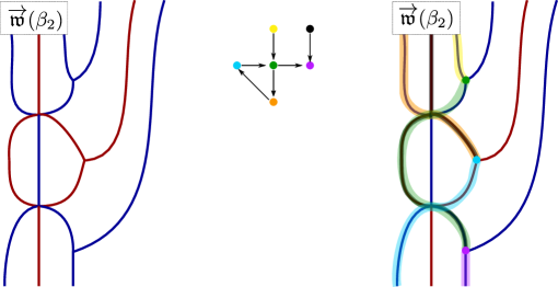
Figure 7. Right inductive weave and cycles for $\beta_{2}\sigma_{i}\sigma_{j}\sigma_{i}$, together with some of its cycles and intersection quiver.

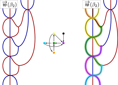
Figure 8. The right inductive weave for $\beta_{2}\sigma_{j}\sigma_{i}\sigma_{j}$, and its intersection quiver. It is easy to see that the quiver here is obtained from that in Figure 7 by mutating at the green vertex. Note that the arrow from the blue to the purple vertex appears only if these cycles are not frozen in the right inductive weave of $\beta$.

Finally, for the relation between the quivers $Q_{\overleftarrow{\mathfrak{w}}(\beta)}$ and $Q_{\overleftarrow{\mathfrak{w}}(\sigma_{i}\beta)}$, we note that $\delta(\beta)=\delta(\sigma_{i}\beta)$ and the weave $\overleftarrow{\mathfrak{w}}(\sigma_{i}\beta)$ can be obtained from the weave $\overleftarrow{\mathfrak{w}}(\beta)$ by adding a new $i$-colored trivalent vertex $v$, which will be frozen. Since the left arm of the trivalent vertex $v$ goes all the way to the top, $v$ is a source in the quiver $Q_{\overleftarrow{\mathfrak{w}}(\sigma_{i}\beta)}$. We thus obtain the following result:

Lemma 4.44.

Let $\beta$ be a braid word such that $\delta(\sigma_{i}\beta)=\delta(\beta)$, and let $v\in\overleftarrow{\mathfrak{w}}(\sigma_{i}\beta)$ be the last trivalent vertex of the weave $\overleftarrow{\mathfrak{w}}(\sigma_{i}\beta)$. Then:

• The vertex $v$ is frozen, and it is a source in $Q_{\overleftarrow{\mathfrak{w}}(\sigma_{i}\beta)}$.

• The quiver $Q_{\overleftarrow{\mathfrak{w}}(\beta)}$ can be obtained from $Q_{\overleftarrow{\mathfrak{w}}(\sigma_{i}\beta)}$ by the following procedure:

  • Remove the frozen vertex $v$.

  • Freeze all vertices that were incident with $v$.

  • Remove possible arrows between frozen vertices.

If otherwise $\beta$ is a braid word such that $\delta(\sigma_{i}\beta)=s_{i}\delta(\beta)$, then the quivers $Q_{\overleftarrow{\mathfrak{w}}(\sigma_{i}\beta)}$ and $Q_{\overleftarrow{\mathfrak{w}}(\beta)}$ coincide.

Remark 4.45.

The appropriate modification of Lemma 4.44 is valid for the right inductive weaves $\overrightarrow{\mathfrak{w}}$. The quiver $Q_{\overrightarrow{\mathfrak{w}}(\beta)}$ is obtained from $Q_{\overrightarrow{\mathfrak{w}}(\beta\sigma_{i})}$ by removing a frozen sink, provided that $\delta(\beta)=\delta(\beta\sigma_{i})$.

5. Construction of cluster structures

In this section we focus on simply laced cases. We introduce the (to be) cluster $\mathcal{A}$-variables, which will be indexed by trivalent vertices of a Demazure weave, study their properties and prove Theorem 1.1.

5.1. Cluster variables in Demazure weaves

Given a Demazure weave $\mathfrak{W}$, let $\gamma_{v}:E(\mathfrak{W})\to\mathbb{Z}_{\geq 0}$ be the cycles associated to the trivalent vertices $v\in\mathfrak{W}$ as in Definition 4.12, and fix variables $z_{1},\ldots,z_{\ell}\in\mathbb{C}$ at the top of $\mathfrak{W}$. We assign a framed flag $B_{r}\in\mathsf{G}/\mathsf{U}$ to every region $r$ on the complement $\mathbb{R}^{2}\setminus\mathfrak{W}$ of the weave as follows. If an edge $e\in\mathfrak{W}$ colored by $s_{i}$ separates two regions $r,r^{\prime}\subset\mathbb{R}^{2}\setminus\mathfrak{W}$, then we require that the corresponding framed flags $B_{r},B_{r^{\prime}}$ are related by $B_{i}(\widetilde{z})\chi_{i}(u)$ for some $u\in\mathbb{C}^{\times}$ and $\widetilde{z}\in\mathbb{C}$. Proposition 3.11 implies that such $u,\widetilde{z}$ are unique.

Theorem 5.1.

Let $\mathfrak{W}$ be a Demazure weave. Then there exists a unique collection of rational functions $A_{v}:=A_{v}(z_{1},\ldots,z_{\ell})\in\mathbb{C}(z_{1},\ldots,z_{\ell})$, indexed by the trivalent vertices of $\mathfrak{W}$, such that for every pair of regions $r,r^{\prime}\subset\mathbb{R}^{2}\setminus\mathfrak{W}$ separated by an edge $e\in\mathfrak{W}$, the flags $B_{r},B_{r^{\prime}}$ are related by

$$B_{i}(\widetilde{z})\chi_{i}\left(\prod_{v}A_{v}^{\gamma_{v}(e)}\right),\quad\mbox{for some }\widetilde{z}\in\mathbb{C}.$$

Proof.

We construct each function $A_{v}$ inductively by scanning the weave $\mathfrak{W}$ from top to bottom. At the top, we have $\gamma_{v}(e)=0$ and the framed flags are simply of the form $\mathsf{U},B_{i_{1}}(z_{1})\mathsf{U},\dots,B_{i_{1}}(z_{1})\cdots B_{i_{\ell}}(z_{\ell})\mathsf{U}$ by Corollary 3.7. This implies that the framed flag on the left unbounded region of $\mathfrak{W}$ is always the standard framed flag $\mathsf{U}$ and, in particular, $\widetilde{z}_{j}=z_{j}$ for $1\leq j\leq\ell$.

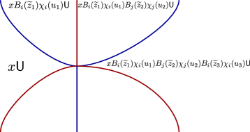
Figure 9. The initial framed flags at the top before scanning a 6-valent vertex.

First, suppose that we arrive at a 6-valent vertex, and that we have the framed flags

$$x\mathsf{U},xB_{i}(\widetilde{z}_{1})\chi_{i}(u_{1})\mathsf{U},xB_{i}(\widetilde{z}_{1})\chi_{i}(u_{1})B_{i}(\widetilde{z}_{2})\chi_{i}(u_{2})\mathsf{U},\mbox{ and }xB_{i}(\widetilde{z}_{1})\chi_{i}(u_{1})B_{i}(\widetilde{z}_{2})\chi_{i}(u_{2})B_{i}(\widetilde{z}_{3})\chi_{i}(u_{3})\mathsf{U}$$

on top, as depicted in Figure 9, where, by induction, $u_{1},u_{2}$ and $u_{3}$ are products of the rational functions $A_{v}$, as in the statement, for the trivalent vertices above. If $v$ is a trivalent vertex, then $\gamma_{v}$ has incoming weights $a,b,c$ and outgoing weights $a^{\prime},b^{\prime},c^{\prime}$ satisfying $a+b=b^{\prime}+c^{\prime}$ and $b+c=a^{\prime}+b^{\prime}$ which implies that the consistency condition in Lemma 3.12 holds. Therefore at this stage $\widetilde{z}^{\prime}_{i}$ are determined by $\widetilde{z}_{i}$ and $A_{v}$, and the framed flags above the 6-valent vertex uniquely determine the framed flags below it.

Second, if we arrive at a 3-valent vertex $v\in\mathfrak{W}$, with $e_{1}$ and $e_{2}$ the two incoming edges and $e_{3}$ the outgoing edge, then $\gamma_{v}(e_{1})=\gamma_{v}(e_{2})=0,\ \gamma_{v}(e_{3})=1.$ The framed version of the identity (10) is:

(17) $$B_{i}(\widetilde{z}_{1})\chi_{i}(u_{1})B_{i}(\widetilde{z}_{2})\chi_{i}(u_{2})=B_{i}(\widetilde{z}^{\prime})\chi_{i}\left(\widetilde{z}_{2}u_{1}u_{2}\right)\varphi_{i}\left(\begin{matrix}1&-\widetilde{z}_{2}^{-1}u_{2}^{-2}\\ 0&1\end{matrix}\right).$$

where $\widetilde{z}^{\prime}=\widetilde{z}_{1}-1/(u_{1}^{2}\widetilde{z}_{2})$. Therefore

$$A_{v}\prod_{v^{\prime}\neq v}A_{v^{\prime}}^{\gamma_{v^{\prime}}(e_{3})}=\widetilde{z}_{2}\prod_{v^{\prime}\neq v}A_{v^{\prime}}^{\gamma_{v^{\prime}}(e_{1})+\gamma_{v^{\prime}}(e_{2})}$$

and

(18) $$A_{v}=\widetilde{z}_{2}\prod_{v^{\prime}\neq v}A_{v^{\prime}}^{\gamma_{v^{\prime}}(e_{1})+\gamma_{v^{\prime}}(e_{2})-\gamma_{v^{\prime}}(e_{3})}.$$

The right hand side of this equality involves only the trivalent vertices $v^{\prime}$ above $v$, and thus we can use Equation (18) to define $A_{v}$ inductively as we scan $\mathfrak{W}$ downwards. ∎

The following two lemmas establish how these functions $A_{v}$ change under weave equivalences, in Lemma 5.2 and mutations, in Lemma 5.3.

Lemma 5.2.

Let $\mathfrak{W}_{1},\mathfrak{W}_{2}$ be the two weaves for $1212$, as in Example 4.11 $($see Fig. 4$)$, and denote their unique trivalent vertices by $v_{1}\in\mathfrak{W}_{1},v_{2}\in\mathfrak{W}_{2}$. Then the variables $A_{v_{1}}(\mathfrak{W}_{1})$ and $A_{v_{2}}(\mathfrak{W}_{2})$ agree.

Proof.

Let us denote both $v_{1}$ and $v_{2}$ by $v$, as the weave determine the index. Suppose that the $\widetilde{z}$-variables on the top are $\widetilde{z}_{1},\widetilde{z}_{2},\widetilde{z}_{3},\widetilde{z}_{4}$ and for $v^{\prime}\neq v$ the incoming edges have multiplicities $a_{v^{\prime}},b_{v^{\prime}},c_{v^{\prime}},d_{v^{\prime}}$. For $\mathfrak{W}_{1}$, the right incoming (red) edge at $v$ has position variable $\widetilde{z}_{4}$, hence

$$A_{v}(\mathfrak{W}_{1})=\widetilde{z}_{4}\prod_{v\neq v^{\prime}}A_{v^{\prime}}^{m_{1}(v^{\prime})}$$

where $m_{1}(v^{\prime})=\left(a_{v^{\prime}}+b_{v^{\prime}}-\min(a_{v^{\prime}},c_{v^{\prime}})\right)+d_{v^{\prime}}-\min(a_{v^{\prime}}+b_{v^{\prime}}-\min(a_{v^{\prime}},c_{v^{\prime}}),d_{v^{\prime}}).$ For $\mathfrak{W}_{2}$, the right incoming (blue) edge at $v$ has position variable

$$\widetilde{z}_{4}\prod_{v^{\prime}\neq v}A_{v^{\prime}}^{b_{v^{\prime}}-c_{v^{\prime}}},$$

by Lemma 3.12). Therefore

$$A_{v}(\mathfrak{W}_{2})=\widetilde{z}_{4}\prod_{v^{\prime}\neq v}A_{v^{\prime}}^{m_{2}(v^{\prime})}$$

where

$$m_{2}(v^{\prime})=(b_{v^{\prime}}-c_{v^{\prime}})+a_{v^{\prime}}+\left(c_{v^{\prime}}+d_{v^{\prime}}-\min(b_{v^{\prime}},d_{v^{\prime}})\right)-$$

$$\min(a_{v^{\prime}},c_{v^{\prime}}+d_{v^{\prime}}-\min(b_{v^{\prime}},d_{v^{\prime}}))=m_{1}(v^{\prime})$$

by Lemma 4.10. Since $m_{1}(v^{\prime})=m_{2}(v^{\prime})$, this shows that $A_{v}(\mathfrak{W}_{1})=A_{v}(\mathfrak{W}_{2})$. ∎

Lemma 5.3.

Let $\mathfrak{W}_{1},\mathfrak{W}_{2}$ be the two weaves for $\sigma_{1}^{3}$, as in Figure 5, and for each of them let $v_{1},v_{2}$ be the two trivalent vertices, $v_{1}$ on top of $v_{2}$. Then the cluster variables $A_{v}=A_{v}(\mathfrak{W}_{1})$ and $\overline{A_{v}}=A_{v}(\mathfrak{W}_{2})$ satisfy

$$A_{v_{1}}\cdot\overline{A_{v_{1}}}=A_{v_{2}}\prod_{v^{\prime}\neq v_{1},v_{2}}A_{v^{\prime}}^{\left[\sharp_{\mathfrak{W_{1}}}(\gamma_{v^{\prime}}\cdot\gamma_{v_{1}})\right]_{+}}+\prod_{v^{\prime}\neq v_{1},v_{2}}A_{v^{\prime}}^{-\left[\sharp_{\mathfrak{W_{1}}}(\gamma_{v^{\prime}}\cdot\gamma_{v_{1}})\right]_{-}}$$

and $A_{v}=\overline{A_{v}}$ for $v\neq v_{1}$.

Proof.

We need to verify the statement for two trivalent vertices $v_{1},v_{2}$. Suppose that the $\widetilde{z}$-variables on the top are $\widetilde{z}_{1},\widetilde{z}_{2},\widetilde{z}_{3}$ and for $v^{\prime}\neq v_{1},v_{2}$ the incoming edges have multiplicities $a_{v^{\prime}},b_{v^{\prime}},c_{v^{\prime}}$.

In $\mathfrak{W}_{1}:(11)1\to 11\to 1$ the position variable at the right incoming edge at $v_{1}$ is $\widetilde{z}_{2}$ and the cluster variable is

$$A_{v_{1}}=\widetilde{z}_{2}\prod_{v^{\prime}}A_{v^{\prime}}^{a_{v^{\prime}}+b_{v^{\prime}}-\min(a_{v^{\prime}},b_{v^{\prime}})}.$$

The position variable at the right incoming edge at $v_{2}$ is $\widetilde{z}_{3}-\widetilde{z}_{2}^{-1}\prod_{v^{\prime}}A_{v}^{-2b_{v^{\prime}}}$. Indeed, we have

$$\varphi_{i}\left(\begin{matrix}1&-\widetilde{z}_{2}^{-1}u_{2}^{-2}\\ 0&1\end{matrix}\right)B_{i}(\widetilde{z}_{3})\chi_{i}(u)=B_{i}(\widetilde{z}_{3}-\widetilde{z}_{2}^{-1}u_{2}^{-2})\chi_{i}(u).$$

Therefore the function $A_{v_{2}}$ at $v_{2}$ equals

$$A_{v_{2}}=(\widetilde{z}_{3}-\widetilde{z}_{2}^{-1}\prod_{v\neq v^{\prime}}A_{v}^{-2b_{v^{\prime}}})A_{v_{1}}\prod_{v^{\prime}}A_{v^{\prime}}^{\min(a_{v^{\prime}},b_{v^{\prime}})+c_{v^{\prime}}-\min(a_{v^{\prime}},b_{v^{\prime}},c_{v^{\prime}})}=$$

$$(\widetilde{z}_{2}\widetilde{z}_{3}-\prod_{v^{\prime}}A_{v}^{-2b_{v^{\prime}}})\prod_{v^{\prime}}A_{v^{\prime}}^{a_{v^{\prime}}+b_{v^{\prime}}+c_{v^{\prime}}-\min(a_{v^{\prime}},b_{v^{\prime}},c_{v^{\prime}})}.$$

For $\mathfrak{W}_{2}:1(11)\to 11\to 1$, the function $\overline{A_{v_{1}}}$ at the top vertex $v_{1}$ is

$$\overline{A_{v_{1}}}=\widetilde{z}_{3}\prod_{v^{\prime}}A_{v^{\prime}}^{b_{v^{\prime}}+c_{v^{\prime}}-\min(b_{v^{\prime}},c_{v^{\prime}})}$$

and by (17)

$$\overline{A_{v_{2}}}=(\widetilde{z}_{2}-\widetilde{z}_{3}^{-1}\prod_{v^{\prime}}A_{v}^{-2b_{v^{\prime}}})\overline{A_{v_{1}}}\prod_{v^{\prime}}A_{v^{\prime}}^{a_{v^{\prime}}+\min(b_{v^{\prime}},c_{v^{\prime}})-\min(a_{v^{\prime}},b_{v^{\prime}},c_{v^{\prime}})}=$$

$$(\widetilde{z}_{2}\widetilde{z}_{3}-\prod_{v^{\prime}}A_{v}^{-2b_{v^{\prime}}})\prod_{v^{\prime}}A_{v^{\prime}}^{a_{v^{\prime}}+b_{v^{\prime}}+c_{v^{\prime}}-\min(a_{v^{\prime}},b_{v^{\prime}},c_{v^{\prime}})}=A_{v_{2}}.$$

Finally,

(19) $$A_{v_{1}}\overline{A_{v_{1}}}=\widetilde{z}_{2}\widetilde{z}_{3}\prod_{v^{\prime}}A_{v^{\prime}}^{a_{v^{\prime}}+2b_{v^{\prime}}+c_{v^{\prime}}-\min(b_{v^{\prime}},c_{v^{\prime}})-\min(a_{v^{\prime}},b_{v^{\prime}})}=\\ A_{v_{2}}\prod_{v^{\prime}}A_{v^{\prime}}^{b_{v^{\prime}}-\min(b_{v^{\prime}},c_{v^{\prime}})-\min(a_{v^{\prime}},b_{v^{\prime}})+\min(a_{v^{\prime}},b_{v^{\prime}},c_{v^{\prime}})}+\prod_{v^{\prime}}A_{v^{\prime}}^{a_{v^{\prime}}+c_{v^{\prime}}-\min(b_{v^{\prime}},c_{v^{\prime}})-\min(a_{v^{\prime}},b_{v^{\prime}})}.$$

By Lemma 4.29 we get $\sharp_{\mathfrak{W}_{1}}(G_{v_{2}}\cdot G_{v_{1}})=-1$ and

$$b_{v^{\prime}}-\min(b_{v^{\prime}},c_{v^{\prime}})-\min(a_{v^{\prime}},b_{v^{\prime}})+\min(a_{v^{\prime}},b_{v^{\prime}},c_{v^{\prime}})=-\left[\sharp_{\mathfrak{W}_{1}}(G_{v^{\prime}}\cdot G_{v_{1}})\right]_{-}$$

and

$$a_{v^{\prime}}+c_{v^{\prime}}-\min(b_{v^{\prime}},c_{v^{\prime}})-\min(a_{v^{\prime}},b_{v^{\prime}})=\left[\sharp_{\mathfrak{W}_{1}}(G_{v^{\prime}}\cdot G_{v_{1}})\right]_{+},$$

concluding that Equation (19) coincides with the equation in the statement. ∎

The transformation described in Lemma 5.3 is precisely a cluster mutation, see Section 2. Therefore, from this moment forward we refer to the functions $A_{v}(\mathfrak{W})$ as the cluster variables associated to a Demazure weave $\mathfrak{W}$. Theorem 5.9 at the end of this section proves that these functions are indeed cluster variables for a cluster structure.

Theorem 5.4.

Let $\mathfrak{W}_{1},\mathfrak{W}_{2}:\beta\to\delta(\beta)$ be two Demazure weaves. Then the collections of functions $A_{v}(\mathfrak{W}_{1})$ and $A_{v}(\mathfrak{W}_{2})$ are related by a sequence of cluster mutations.

Proof.

By Lemma 4.4 any two such Demazure weaves are related by a sequence of equivalence moves and weave mutations. By Lemma 5.2, the equivalence moves for weaves do not change the collection $A_{v}$ and by Lemma 5.3 a weave mutation corresponds to a cluster mutation. ∎

5.2. Cluster variables in inductive weaves

In an inductive weave, the procedure for computing the cluster variables $A_{v}$ from Theorem 5.1 can be made more explicit, as we now describe. At each trivalent vertex of a left inductive weave, the left incoming edge goes all the way to the top, but the right incoming edge may be contained in some cycles.

Definition 5.5.

Let $\mathfrak{W}$ be a left inductive weave and $v,v^{\prime}\in\mathfrak{W}$ trivalent vertices. By definition, $v^{\prime}$ is said to cover $v$ if $\gamma_{v^{\prime}}(e_{r})\neq 0$ where $e_{r}$ is the right incoming edge of $v$.

Theorem 5.6.

Let $\mathfrak{W}$ be a left inductive weave and $v\in\mathfrak{W}$ a trivalent vertex with color $i\in\mathsf{D}$ and $\mathsf{U}_{1},\mathsf{U}_{2}\in\mathsf{G}/\mathsf{U}$ the framed flags associated to $\mathfrak{W}$ to the left and right of this trivalent vertex, respectively. Then:

• The $\widetilde{z}$-variable $s_{v}$ on the right incoming edge of $v$ agrees with the corresponding $z$-variable.

• The cluster variable $A_{v}(\mathfrak{W})$ associated to $v\in\mathfrak{W}$ satisfies the equation

  $$A_{v}=s_{v}\cdot\prod_{v^{\prime}\ \mathrm{covers}\ v}A_{v^{\prime}}^{\gamma_{v^{\prime}}(e_{r})}.$$

• We have the equality

  $$A_{v}=\Delta_{\omega_{i}}(\mathsf{U}_{1},\mathsf{U}_{2}),$$

  where $\Delta_{\omega_{i}}$ is the generalized principal minor associated to the fundamental weight $\omega_{i}$.

Part $(3)$ also holds for a right inductive weave.

Proof.

For Part (1), all edges $e$ of the weave to the left of $v$, including the left incoming edge at $v$, go all the way to the top, and thus we have $\gamma_{v^{\prime}}(e)=0$ and $u_{e}=1$. On the right incoming edge at $v$, we have the matrix $B_{i}(\widetilde{z})\chi_{i}(u)$ and, if we move $\chi_{i}(u)$ to the right as in Lemma 3.13, then $\widetilde{z}$ would not change. Therefore $\widetilde{z}=z$.

For Part (2), let $e_{1},e_{2}$ and $e_{3}$ be the left incoming, the right incoming, and the outgoing edge of $v$, respectively. We have $\gamma_{v^{\prime}}(e_{1})=\gamma_{v^{\prime}}(e_{3})=0$ for all $v^{\prime}\neq v$ and $\gamma_{v^{\prime}}(e_{2})\neq 0$ if and only if $v^{\prime}$ covers $v$, so the result follows from Equation (18).

For Part (3), we get $\Delta_{\omega_{i}}(\mathsf{U}_{1},\mathsf{U}_{2})=\prod_{v^{\prime}}A_{v^{\prime}}^{\gamma_{v^{\prime}}(e_{3})}$. By the above, we have $\gamma_{v^{\prime}}(e_{3})=\delta_{v,v^{\prime}}$, which implies the result. The proof for a right inductive weave is identical. ∎

Next, we consider the right inductive weave $\overrightarrow{\mathfrak{w}}(\Delta\beta)$, constructed in Section 4.8, and compare the variables $A_{v}(\overrightarrow{\mathfrak{w}}(\Delta\beta))$, for the trivalent vertices $v\in\overrightarrow{\mathfrak{w}}(\Delta\beta)$, with those cluster variables coming from the cluster structure on $\operatorname{Conf}(\beta)\cong X(\Delta\beta)$, as defined in [68] and described in Section 3.7 above. We will denote by $w$ the variables corresponding to the crossings of $\Delta$, and by $z$ the variables corresponding to the crossings of $\beta$.

As explained in Section 4.8, the trivalent vertices of $\overrightarrow{\mathfrak{w}}(\Delta\beta)$ correspond to the letters of $\beta=\sigma_{i_{1}}\cdots\sigma_{i_{r}}$. Denote by $A_{k}=A_{v_{k}}(\overrightarrow{\mathfrak{w}}(\Delta\beta))$, $1\leq k\leq r$, the cluster variables, constructed in Theorem 5.1 and associated to the corresponding trivalent vertices in $\overrightarrow{\mathfrak{w}}(\Delta\beta)$. Similarly, denote by $\widetilde{A}_{k}$ the rational function (in fact, polynomial) defined in Section 3.7, i.e. $\widetilde{A}_{k}(z_{1},\dots,z_{r}):=\Delta_{\omega_{i_{k}}}(B_{i_{1}}(z_{1})\cdots B_{i_{k}}(z_{k}))$.

Proposition 5.7.

In a right inductive weave, we have $A_{k}=\widetilde{A}_{k}$ for all $1\leq k\leq r$.

Proof.

For that, we use the description of the variables $A_{k},\widetilde{A}_{k}$ in terms of the distances between framed flags, as follows. First, consider a configuration of flags

$\in X(\Delta\beta)$

where $\Delta=\sigma_{j_{1}}\cdots\sigma_{j_{\ell}}$. This admits a unique lift with the condition that $\mathsf{B}$ gets lifted to $\mathsf{U}$; denote by $\mathsf{U}_{s}$ the lift of $\mathsf{B}_{s}$. Let $k$ be such that $1\leq k\leq r$ and $i_{k}=i$. Then, by definition, $\widetilde{A}_{k}=\Delta_{\omega_{i}}(\mathsf{U},\mathsf{U}_{\ell+k})$. The function $A_{k}$ is given as follows; let $\mathsf{U}^{\prime},\mathsf{U}^{\prime\prime}$ be the decorated flags to the left and right of the trivalent vertex corresponding to $\sigma_{i_{k}}$, and note that by the definition of the right inductive weave $\overrightarrow{\mathfrak{w}}(\Delta\beta)$ we have $\mathsf{U}^{\prime\prime}=\mathsf{U}_{\ell+k}$, see Figure 10. Theorem 5.6 implies $A_{k}=\Delta_{\omega_{i}}(\mathsf{U}^{\prime},\mathsf{U}_{\ell+k})$.

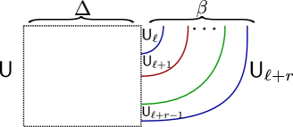
Figure 10. The right inductive weave for $\Delta\beta$ together with its collection of framed flags. Every horizontal slice inside the rectangle is a reduced word for $w_{0}$.

It thus suffices to show that $\Delta_{\omega_{i}}(\mathsf{U},\mathsf{U}_{\ell+k})=\Delta_{\omega_{i}}(\mathsf{U}^{\prime},\mathsf{U}_{\ell+k})$. Consider a slice of the weave right below the trivalent vertex corresponding to $\sigma_{i_{k}}$, which gives a sequence of framed flags $\mathsf{A},\mathsf{A_{1}},\dots,\mathsf{A_{\ell}}$, with $\mathsf{A}=\mathsf{U}$ and $\mathsf{A_{\ell}}=\mathsf{U}_{\ell+k}$, see Figure 10. The required equality now follows by [44, Lemma-Definition 8.3] upon the observation that, since the weave at this point spells a reduced decomposition of $\Delta$, the only appearance of the simple root $\alpha_{i}$ in the sequence $\beta_{\mathbf{i},k}$ (cf. [44, Lemma-Definition 8.3]) is at the last step. ∎

Corollary 5.8.

Let $\beta\in\operatorname{Br}_{W}^{+}$ be a positive braid word. Then

$$\mathbb{C}[X(\Delta\beta)]\cong\mathrm{up}(Q_{\overrightarrow{\mathfrak{w}}(\Delta\beta)})=\mathcal{A}(Q_{\overrightarrow{\mathfrak{w}}(\Delta\beta)}).$$

In fact, $\mathbb{C}[X(\Delta\beta)]\cong\mathrm{up}(Q_{\mathfrak{w}})=\mathcal{A}(Q_{\mathfrak{w}})$ where $\mathfrak{w}:\Delta\beta\to\Delta$ is any Demazure weave.

Proof.

By Proposition 5.7 and Corollary 4.42, the first statement is equivalent to [68, Theorem 3.45]. The second statement follows from Theorems 4.31 and 5.4 above. ∎

5.3. Existence of upper cluster structures

Theorem 1.1, in the simply-laced case, is proven in two steps at this stage. First, for any braid $\beta\in\operatorname{Br}_{W}^{+}$, we now show that the algebra of regular functions $\mathbb{C}[X(\beta)]$ is an upper cluster algebra. Second, we prove $\mathcal{A}=\mathcal{U}$ in Subsection 5.4. The main result of this subsection is the following:

Theorem 5.9.

Let $\beta\in\operatorname{Br}_{W}^{+}$ be a positive braid word, $\overleftarrow{\mathfrak{w}}(\beta)$ the left inductive weave and $Q_{\overleftarrow{\mathfrak{w}}(\beta)}$ its corresponding quiver. Then we have

$$\mathbb{C}[X(\beta)]\cong\mathrm{up}(Q_{\overleftarrow{\mathfrak{w}}(\beta)}).$$

Remark 5.10.

The use of the left inductive weave $\overleftarrow{\mathfrak{w}}(\beta)$ simplies part of the arguments in the proof of Theorem 5.9. Nevertheless, by Theorems 4.31 and 5.4, we then also have $\mathbb{C}[X(\beta)]\cong\mathrm{up}(Q_{\mathfrak{W}})$ for $\mathfrak{W}:\beta\to\delta(\beta)$ any Demazure weave.

In order to prove Theorem 5.9 we need the following preparatory lemmata, describing how the braid variety $X(\beta)$ and the quiver $Q_{\overleftarrow{\mathfrak{w}}(\beta)}$ change upon adding a new crossing on the left of $\beta$. The following is a more precise version of Lemma 3.4:

Lemma 5.11.

Let $\beta$ be a positive braid word, $\delta=\delta(\beta)$ its Demazure product, and let $z=z_{1}\in\mathbb{C}[X(\sigma_{i}\beta)]$ be the $($restriction of the$)$ coordinate associated to the first crossing in $\sigma_{i}\beta$. Then the following holds:

• If $\delta(\sigma_{i}\beta)=\sigma_{i}\delta$, then $z=0$ on the braid variety $X(\sigma_{i}\beta)$ and $X(\sigma_{i}\beta)\cong X(\beta)$.

• If $\delta(\sigma_{i}\beta)=\delta$, then we have an isomorphism

  $$X(\beta)\times\mathbb{C}^{*}\cong\{p\in X(\sigma_{i}\beta):z(p)\neq 0\}\subset X(\sigma_{i}\beta).$$

Proof.

For Part (1), note that the variety $X(\sigma_{i}\beta)$ is cut out by the conditions

$$(\sigma_{i}\delta)^{-1}B_{\beta\sigma_{i}}(z,z_{2},\ldots,z_{\ell(\beta)+1})=U,\quad B_{\beta\sigma_{i}}(z,z_{2},\ldots,z_{\ell(\beta)+1})=B_{i}(z)B_{\beta}=\sigma_{i}\delta U=B_{\sigma_{i}\delta}(0,\ldots,0)U$$

for some $U\in B$. We can uniquely write $B_{\beta}=B_{w}(a_{1},\ldots,a_{\ell(w)})U^{\prime}$ for some reduced expression $w\leq\delta$ and some $a_{i}\in\mathbb{C}$. If we had $w<\delta$, then $\sigma_{i}w<\sigma\delta$, but we have

$$B_{i}(z)B_{\beta}=B_{\sigma_{i}w}(z,a_{1},\ldots,a_{\ell(w)})U^{\prime},$$

which is a contradiction. For $w=\delta$, we have $z=a_{1}=\ldots=a_{\ell(\delta)}=0$, and so $U=U^{\prime}$ and $B_{\beta}=\delta U$.

For Part (2), let us assume $z\neq 0$. Then we can decompose

(20) $$\left(\begin{matrix}z&-1\\ 1&0\\ \end{matrix}\right)=\left(\begin{matrix}z&0\\ 1&z^{-1}\end{matrix}\right)\left(\begin{matrix}1&-z^{-1}\\ 0&1\\ \end{matrix}\right),$$

and factor $B_{i}(z)=L_{i}(z)U_{i}(z)$ accordingly. Now we also have

$$\delta^{-1}B_{i}(z)B_{\beta}=\delta^{-1}L_{i}(z)U_{i}(z)B_{\beta}=U^{\prime}\delta^{-1}\widetilde{B_{\beta}}U^{\prime\prime}$$

where $U^{\prime},U^{\prime\prime}$ are in $\mathsf{B}$. Indeed, $U_{i}(z)B_{\beta}=\widetilde{B_{\beta}}U^{\prime\prime}$ by Corollary 3.9, and $\delta^{-1}L_{i}(z)=U^{\prime}\delta^{-1}$ since $\ell(\sigma_{i}\delta)<\ell(\delta)$ and $\ell(\delta^{-1}\sigma_{i})<\ell(\delta^{-1})$. Therefore, for a fixed $z\neq 0$, the matrix $\delta^{-1}B_{i}(z)B_{\beta}$ is in $\mathsf{B}$ if and only if $\delta^{-1}\widetilde{B_{\beta}}$ is in $\mathsf{B}$, and the result follows. ∎

In the notation of Lemma 5.11, the next statement follows from the construction:

Lemma 5.12.

Let $\beta$ be a positive braid word, $\delta=\delta(\beta)$ its Demazure product, and assume $\delta(\sigma_{i}\beta)=\sigma_{i}\delta$. Then the inductive weave $\overleftarrow{\mathfrak{w}}(\sigma_{i}\beta)$ is obtained from $\overleftarrow{\mathfrak{w}}(\beta)$ by adding a disjoint line, and the cycles and cluster variables for $X(\sigma_{i}\beta)$ and $X(\beta)$ agree.

For the the case $\delta(\sigma_{i}\beta)=\delta$, the inductive weave $\overleftarrow{\mathfrak{w}}(\sigma_{i}\beta)$ is obtained by adding a trivalent vertex $v$ at the bottom left corner of $\overleftarrow{\mathfrak{w}}(\beta)$. Then the isomorphism $X(\beta)\times\mathbb{C}^{*}\cong\{z\neq 0\}$ from Lemma 5.11(b) can be extended to the weave $\overleftarrow{\mathfrak{w}}(\beta)$ as in Lemma 4.2.

Lemma 5.13.

Let $\beta\in\operatorname{Br}^{+}_{W}$ be a positive braid word with $\delta(\sigma_{i}\beta)=\delta(\beta)$, $i\in\mathsf{D}$, and $v\in\overleftarrow{\mathfrak{w}}(\sigma_{i}\beta)$ the trivalent vertex for $\sigma_{i}$. Let $z,a_{1},\ldots,a_{\ell}$ be the variables associated to the slice of $\overleftarrow{\mathfrak{w}}(\sigma_{i}\beta)$ above $v$, read left-to-right, so that $z$ and $a_{1}$ are the incoming variables at the vertex $v$. Then we have:

• $a_{1}=z^{-1},\ a_{2}=\ldots=a_{\ell}=0.$

• The cycles and the quiver for $\overleftarrow{\mathfrak{w}}(\sigma_{i}\beta)$ and $\overleftarrow{\mathfrak{w}}(\beta)$ agree, up to removing the vertex for $v$. The frozen vertices of the quiver for $\overleftarrow{\mathfrak{w}}(\beta)$ are precisely the frozen vertices of the quiver for $\overleftarrow{\mathfrak{w}}(\sigma_{i}\beta)$ together with those mutable vertices that have an arrow to the vertex for $v$.

• The cluster variables for $\overleftarrow{\mathfrak{w}}(\sigma_{i}\beta)$, except for $A_{v}$, and the cluster variables for $\overleftarrow{\mathfrak{w}}(\beta)$ agree.

• The variable $z$ is a cluster monomial for $\overleftarrow{\mathfrak{w}}(\sigma_{i}\beta)$.

Proof.

For Part (1), since the first output variable for the weave vanishes, we have $z-a_{1}^{-1}=0$ and $a_{1}=z^{-1}$. For the other output variables, we use the change of variables prescribed by Lemma 4.2. On the top of $\overleftarrow{\mathfrak{w}}(\beta)$, we use the change of variables from Lemma 5.11(b) which is determined by the matrix $U_{i}(z)$ from (20). At the bottom of $\overleftarrow{\mathfrak{w}}(\beta)$, we can write $\delta=\sigma_{i}\gamma$, then

$$\delta^{-1}U_{i}(z)B_{\delta}(a_{1},\ldots,a_{\ell})=\delta^{-1}U_{i}(z)B_{i}(a_{1})B_{\gamma}(a_{2},\ldots,a_{\ell})=$$

$$\delta^{-1}\varphi_{i}\left(\begin{matrix}1&-z^{-1}\\ 0&1\\ \end{matrix}\right)\varphi_{i}\left(\begin{matrix}z^{-1}&-1\\ 1&0\\ \end{matrix}\right)B_{\gamma}(a_{2},\ldots,a_{\ell})=\delta^{-1}\left(\begin{matrix}0&-1\\ 1&0\\ \end{matrix}\right)B_{\gamma}(a_{2},\ldots,a_{\ell})=$$

$$\gamma^{-1}B_{\gamma}(a_{1},\ldots,a_{\ell-1})$$

This belongs to the Borel subgroup if and only if $a_{1}=\ldots=a_{\ell-1}=0$. This concludes Part (1). Part (2) is immediate by construction, see also Lemma 4.44. Part (3) follows from Lemma 4.2. Indeed, the matrix $U_{i}(z)$ has a 1 on each diagonal entry, so it does not change the variable at the right incoming edge of any trivalent vertex. By Equation (18), this implies that the cluster variables do not change as well.

For Part (4), note that the cycles in the weave $\overleftarrow{\mathfrak{w}}(\sigma_{i}\beta)$ can approach $v$ only from the right. If the cycle corresponding to the cluster variable $A_{i}$ has weight $w_{i}$ on the right incoming edge at $v$, then it has weight $\min(w_{i},0)=0$ on the outgoing edge. By Equation (18), see also Theorem 5.6, we have

$$A_{v}=a_{1}\prod_{i}A_{i}^{w_{i}}=z^{-1}\prod_{i}A_{i}^{w_{i}},$$

and therefore

(21) $$z=A_{v}^{-1}\prod_{i}A_{i}^{w_{i}}.$$

∎

Lemma 5.14.

Let $\beta\in\operatorname{Br}^{+}_{W}$ be a positive braid word with $\delta(\sigma_{i}\beta)=\delta(\beta)$, $i\in\mathsf{D}$, and $v\in\overleftarrow{\mathfrak{w}}(\sigma_{i}\beta)$ the trivalent vertex for $\sigma_{i}$. Suppose that the cluster variables $A_{u}$ for the braid variety $X(\sigma_{i}\beta)$ are regular functions, $A_{u}\in\mathbb{C}[X(\sigma_{i}\beta)]$, $u\in\overleftarrow{\mathfrak{w}}(\sigma_{i}\beta)$ trivalent vertices with $u\neq v$, and that the cluster variable $A_{v}$ associated to $v$ is invertible. Then all cluster variables for $X(\beta)$ are regular functions, and all cluster variables with nonzero weight at $v$ are invertible.

Proof.

By Lemma 5.13 all cluster variables for $\beta$ are regular on $X(\beta)\times\mathbb{C}^{*}$ and do not depend on $z$. Therefore all cluster variables are regular on $X(\beta)$. Furthermore, by assumption, $A_{v}$ is invertible on $X(\sigma_{i}\beta)$, and $z=A_{v}^{-1}\prod_{i}A_{i}^{w_{i}}$ is invertible on $X(\beta)\times\mathbb{C}^{*}$. Since a product of regular functions is invertible if and only if each factor is invertible, we conclude that the cluster variables $A_{i}$ are invertible on $X(\beta)$ provided that $w_{i}>0$. ∎

The following lemma shows that Theorem 5.9 holds for a braid word $\sigma_{i}\beta$ if it holds for the braid word $\sigma_{i}\beta$, for any $i\in\mathsf{D}$.

Lemma 5.15.

Let $\beta\in\operatorname{Br}_{W}^{+}$ be a positive braid word and suppose that there exists an isomorphism $\mathbb{C}[X(\sigma_{i}\beta)]\cong\mathrm{up}(Q_{\overleftarrow{\mathfrak{w}}(\sigma_{i}\beta)})$ for some $i\in\mathsf{D}$. Then we have

$$\mathbb{C}[X(\beta)]\cong\mathrm{up}(Q_{\overleftarrow{\mathfrak{w}}(\beta)}).$$

Proof.

The case that $\delta(\sigma_{i}\beta)=s_{i}\delta(\beta)$ follows by Lemma 5.11(a) and Lemma 5.12. Thus, we assume that $\delta(\sigma_{i}\beta)=\delta(\beta)$, and use the notation of Lemma 5.13. By the same Lemma 5.13, we can identify $X(\beta)$ with the algebraic subvariety $\{p\in X(\sigma_{i}\beta):z(p)=1\}\subseteq X(\sigma_{i}\beta)$. By Equation (21), we also identify the algebra of regular functions $\mathbb{C}[X(\beta)]$ with the algebra obtained from $\mathbb{C}[X(\sigma_{i}\beta)]$ by freezing all cluster variables that have an arrow to the last variable in $Q_{\overleftarrow{\mathfrak{w}}(\sigma_{i}\beta)}$ and, moreover, specializing $A_{v}=\prod A_{i}^{-w_{i}}$.

Note that when we freeze all variables adjacent to the last (frozen) variable in $Q_{\overleftarrow{\mathfrak{w}}(\sigma_{i}\beta)}$ the quiver becomes disconnected and the specialization $A_{v}=\prod A_{i}^{-w_{i}}$ simply deletes the isolated vertex corresponding to $v$ from the quiver. Since $Q_{\overleftarrow{\mathfrak{w}}(\beta)}$ is obtained from $Q_{\overleftarrow{\mathfrak{w}}(\sigma_{i}\beta)}$ by exactly this procedure, see Lemma 5.13(b), we obtain the following inclusion, cf. [62, Proposition 3.1]:

$$\mathbb{C}[X(\beta)]\subseteq\mathrm{up}(Q_{\overleftarrow{\mathfrak{w}}(\beta)})$$

Let us show the reverse inclusion. By Lemma 5.13, the cluster variables for $\overleftarrow{\mathfrak{w}}(\sigma_{i}\beta)$, without $A_{v}$, and the cluster variables for $\overleftarrow{\mathfrak{w}}(\beta)$ agree. Every mutable variable in $\overleftarrow{\mathfrak{w}}(\beta)$ is not to the last vertex in $Q_{\overleftarrow{\mathfrak{w}}(\sigma_{i}\beta)}$ and it follows that in $\mathbb{C}[X(\beta)]$ we can mutate at all these variables and still get regular functions. Now, by [17, Lemma 4.9], the algebra $\mathbb{C}[X(\beta)]$ is a UFD and by [41, Theorem 3.1], all cluster variables are irreducible in $\mathrm{up}(Q_{\overleftarrow{\mathfrak{w}}(\beta)})$ and thus they are also irreducible in $\mathbb{C}[X(\beta)]$. Appealing once more to factoriality of $X(\beta)$, as well as to its smoothness, we use [28, Corollary 6.4.6] (see Remark 6.4.4 in loc. cit) to conclude

$$\mathrm{up}(Q_{\overleftarrow{\mathfrak{w}}(\beta)})\subseteq\mathbb{C}[X(\beta)].$$

∎

Proof of Theorem 5.9.

By Corollary 5.8, Theorem 5.9 holds for words of the form $\Delta\beta$, $\beta\in\operatorname{Br}_{W}^{+}$ a positive braid word. Then the general result follows by Lemma 5.15, as we can use it to delete each crossing of $\Delta$, left to right, until we obtain the desired result for $\beta$. ∎

5.4. Cyclic rotations and quasi-cluster transformations

In order to show the equality $\mathrm{up}(Q_{\overleftarrow{\mathfrak{w}}(\beta)})=\mathcal{A}(Q_{\overleftarrow{\mathfrak{w}}(\beta)})$ we use the notion of a quasi-equivalence of cluster structures, following C. Fraser’s work [32] and see also [33], as follows. Given a seed $\Sigma$ and a mutable variable $A_{i}$, consider the following ratio, which is the quotient of the two terms in the mutation formula from Equation (2):

(22) $$y_{i}=\frac{\prod_{\varepsilon_{ij}>0}A_{j}^{\varepsilon_{ij}}}{\prod_{\varepsilon_{ij}<0}A_{j}^{-\varepsilon_{ij}}}=\prod_{j}A_{j}^{\varepsilon_{ij}}.$$

Let $\Sigma,\Sigma^{\prime}$ be two seeds in different cluster structures. By definition, the seeds $\Sigma,\Sigma^{\prime}$ are called quasi-equivalent if they satisfy the following conditions:

• The groups of monomials in frozen variables $\Sigma,\Sigma^{\prime}$ agree. In other words, the frozen variables in $\Sigma^{\prime}$ are monomials in the frozen variables in $\Sigma$, and vice versa.

• The mutable variables in $\Sigma^{\prime}$ differ from the mutable variables in $\Sigma$ by monomials in frozens.

• The ratios (22) in $\Sigma$ and in $\Sigma^{\prime}$ agree for any mutable variable.

A key result [32, Proposition 2.3] is that quasi-equivalence commutes with mutations; if we mutate two quasi-equivalent seeds in their respective vertices, the new seeds will be quasi-equivalent as well.

Let us now prove the equality $\mathrm{up}(Q_{\mathfrak{w}})=\mathcal{A}(Q_{\mathfrak{w}})$ by studying cyclic rotations of braids words. Consider two positive braids words $\beta=\sigma_{i_{1}}\cdots\sigma_{i_{\ell}}$ and $\beta^{\prime}=\sigma_{i_{2}}\cdots\sigma_{i_{\ell}}\sigma_{j}$, with $\delta(\beta)=\delta(\beta^{\prime})=w_{0}$ and $s_{i}w_{0}=w_{0}s_{j}$. Then Lemma 3.10 implies that

• The braid varieties $X(\beta)$ and $X(\beta^{\prime})$ are isomorphic,

• The isomorphism in Part (a) changes the variables as follows:

  $$(z_{1},z_{2},\ldots,z_{\ell})\mapsto(z_{2},\ldots,z_{\ell},z^{\prime}),\quad\mbox{ for some }z^{\prime}:=z^{\prime}(z_{1},z_{2},\ldots,z_{\ell}).$$

The goal is to show that this isomorphism is in fact a quasi-cluster transformation, when we consider the upper cluster structures on $X(\beta)$ and $X(\beta^{\prime})$ built in Theorem 5.9. Let $\mathfrak{W}$ be an arbitrary Demazure weave for $\sigma_{i_{2}}\cdots\sigma_{i_{\ell}}$ and $\mathfrak{W}_{1}$, $\mathfrak{W}_{2}$ its extensions using $\sigma_{i}$ and $\sigma_{j}$ respectively, as depicted in Figure 11.

Figure 11. The weaves $\mathfrak{W}_{1}$ and $\mathfrak{W}_{2}$. We assume that the southern boundary of $\mathfrak{W}$ is a reduced word for $w_{0}$ starting with $s_{i}$. The equality $s_{i}w_{0}=w_{0}s_{j}$ assures that we can bring the blue string on the left to the right using Reidemeister moves, as in $\mathfrak{W}_{2}$.

Lemma 5.16.

Suppose that a cycle $C_{i}$ enters a 6-valent vertex $v$ with weights $(w_{i},0,0)$, $z_{1},u_{1},z_{2},u_{2},z_{3},u_{3}$ are input variables as in Figure 9, and $z^{\prime}_{1},u^{\prime}_{1},z^{\prime}_{2},u^{\prime}_{2},z^{\prime}_{3},u^{\prime}_{3}$ are output variables. Then $z^{\prime}_{3},u^{\prime}_{3}$ are related to $z_{1},u_{1}$ by monomials in $A_{j}$ and

$$(z_{1}u_{1})^{-w_{i}}=(z^{\prime}_{3}u^{\prime}_{3})^{-w_{i}}\prod_{j}A_{j}^{\sharp_{v}(C_{i}\cdot C_{j})}.$$

Proof.

The cycle $C_{i}$ exits $v$ with weights $(0,0,w_{i})$. Suppose that other cycles $C_{j}$ ($j\neq i$) enter the $6$-valent vertex with weights $(a_{j},b_{j},c_{j})$ and exit with weights $(a^{\prime}_{j},b^{\prime}_{j},c^{\prime}_{j})$. By Example 4.18 we obtain $\sharp_{v}(C_{i}\cdot C_{j})=w_{i}(b^{\prime}_{j}-c_{j})=w_{i}(b_{j}-a^{\prime}_{j})$.

By Lemma 3.12 we have $z^{\prime}_{3}=z_{1}\frac{u^{\prime}_{2}}{u^{\prime}_{1}}=z_{1}\prod{A_{j}}^{b^{\prime}_{j}-a^{\prime}_{j}}$, and by construction we have $u_{1}=A_{i}^{w_{i}}\prod A_{j}^{a_{j}},u^{\prime}_{3}=A_{i}^{w_{i}}\prod A_{j}^{c^{\prime}_{j}}$. Now

$$(z_{1}u_{1})^{-w_{i}}=z_{1}^{-w_{i}}A_{i}^{-w_{i}^{2}}\prod_{j}A_{j}^{-w_{i}a_{j}}$$

while

$$(z^{\prime}_{3}u^{\prime}_{3})^{-w_{i}}\prod_{j}A_{j}^{w_{i}(b_{j}-a^{\prime}_{j})}=z_{1}^{-w_{i}}\prod_{j}A_{j}^{-w_{i}(b^{\prime}_{j}-a^{\prime}_{j})}A_{i}^{-w^{2}_{i}}\prod A_{j}^{-w_{i}c^{\prime}_{j}}\prod_{j}A_{j}^{w_{i}(b_{j}-a^{\prime}_{j})}=z_{1}^{-w_{i}}A_{i}^{-w_{i}^{2}}\prod_{j}A_{j}^{-w_{i}a_{j}},$$

where we have used the identity $b^{\prime}_{j}+c^{\prime}_{j}=a_{j}+b_{j}$. ∎

Theorem 5.17.

Let $\mathfrak{W}_{1}$, $\mathfrak{W}_{2}$ as in Figure 11. Then:

• All the cluster variables for $\mathfrak{W}_{1}$ and $\mathfrak{W}_{2}$ agree, except for the last variables.

• The last cluster variables for $\mathfrak{W}_{1}$ and $\mathfrak{W}_{2}$ are inverse to each other, up to monomials in frozens.

• The cluster variables in $\mathfrak{W}_{1}$ and $\mathfrak{W}_{2}$ are related by a quasi-cluster transformation.

Proof.

Part (1) holds by construction, as Lemma 3.10 shows that the variables $z_{2},\ldots,z_{\ell}$ do not change.

For Part (2), let $v_{1}$ and $v_{2}$ denote the bottom trivalent vertices of $\mathfrak{W}_{1}$ and $\mathfrak{W}_{2}$, respectively. Let $\widetilde{z_{1}}=z_{1}$ and $\widetilde{z_{2}}$ denote the variables at the left and right incoming edges of $v_{1}$, while $\widetilde{z_{3}}$ and $\widetilde{z_{4}}$ denote the variables at the left and right incoming edges of $v_{2}$. Note that $\widetilde{z_{4}}$ may differ from the variable $z^{\prime}$ at the top of the weave. For $\mathfrak{W}_{1}$, we have $A_{v_{1}}=\widetilde{z_{2}}u$ and the right incoming edge carries the matrix $B_{i}(\widetilde{z_{2}})\chi_{i}(u)$, where $u=\prod_{i}A_{i}^{w_{i}}$. For $\mathfrak{W}_{2}$, the left incoming edge carries the matrix $B_{j}(\widetilde{z_{3}})\chi_{j}(u^{\prime})$ and by Lemma 5.16 the variables $\widetilde{z_{3}}$ and $\widetilde{z_{2}}$ (resp. $u^{\prime}$ and $u$) differ by a monomial in frozen variables. Equation (17) implies

$$\widetilde{z_{3}}-(u^{\prime})^{-2}\widetilde{z_{4}}^{-1}=0,\quad\mbox{i.e. }\widetilde{z_{4}}=(u^{\prime})^{-2}(\widetilde{z_{3}})^{-1}.$$

The cluster variable $A_{v_{2}}$ equals $\widetilde{z_{4}}u^{\prime}=(\widetilde{z_{3}}u^{\prime})^{-1}$ and thus it agrees with $(\widetilde{z_{2}}u)^{-1}=A_{v_{1}}^{-1}$ up to a monomial in frozen variables, as required.

For part (3), we need to verify that the ratios (22) agree. Let $C_{i}$ be a mutable cycle. In the weave $\mathfrak{W}_{1}$ we have

$$\sharp_{\mathfrak{W}_{1}}(C_{i}\cdot C_{v_{1}})=\left|\begin{matrix}1&1&1\\ 0&0&w_{i}\\ 0&1&0\\ \end{matrix}\right|=-w_{i},$$

so we obtain the equality

$$y_{i}=A_{v_{1}}^{-w_{i}}\prod_{j}A_{j}^{\sharp(C_{i}\cdot C_{j})}=(\widetilde{z_{2}}u)^{-w_{i}}\prod_{j}A_{j}^{\sharp_{\mathfrak{W}_{1}}(C_{i}\cdot C_{j})}.$$

By Lemma 5.16 this equals

$$(\widetilde{z_{3}}u^{\prime})^{-w_{i}}\prod_{j}A_{j}^{\sharp_{\mathfrak{W}_{2}}(C_{i}\cdot C_{j})}.$$

In $\mathfrak{W}_{2}$, the last cluster variable is $(\widetilde{z_{3}}u^{\prime})^{-1}$ and the corresponding intersection index with $C_{i}$ equals

$$\left|\begin{matrix}1&1&1\\ w_{i}&0&0\\ 0&1&0\\ \end{matrix}\right|=w_{i},$$

from which the result follows. ∎

Let us remark that quasi-cluster transformations may not preserve the mutation class of the iced quiver $Q$, as the following example illustrates.

Example 5.18.

Consider the braid word $\beta=\sigma_{1}\sigma_{1}\sigma_{2}\sigma_{2}\sigma_{1}\sigma_{1}\sigma_{2}$. The quiver $Q_{\mathfrak{W}}$ for any weave $\mathfrak{W}:\beta\to\delta(\beta)$ has three frozen variables, one mutable variables and it is of the form

$$Q_{\mathfrak{W}}=\square\to\bullet\to\square\qquad\square.$$

For $\beta^{\prime}=\sigma_{1}\sigma_{1}\sigma_{1}\sigma_{2}\sigma_{2}\sigma_{1}\sigma_{1}$ and its right inductive weave $\overrightarrow{\mathfrak{w}}(\beta^{\prime})$ the quiver reads

$$Q_{\overrightarrow{\mathfrak{w}}(\beta^{\prime})}=\bullet\to\square\qquad\square\qquad\square.$$

Remark 5.19.

Let $Q^{\operatorname{uf}}$ denote the full subquiver whose vertices are the mutable vertices of $Q$, and $\mathfrak{W}_{1},\mathfrak{W}_{2}$ be weaves as in Figure 11. Then we have an equality $Q_{\mathfrak{W}_{1}}^{\operatorname{uf}}=Q_{\mathfrak{W}_{2}}^{\operatorname{uf}}$.

5.5. Theorem 1.1 in simply-laced case

Theorem 5.17 allows us to conclude $\mathcal{A}=\mathcal{U}$, as follows:

Corollary 5.20.

Let $\beta\in\operatorname{Br}_{W}^{+}$ be a positive braid word of length $r=\ell(\beta)$ and consider the upper cluster structure on $\mathbb{C}[X(\beta)]$ for $X(\beta)\subset\operatorname{Spec}\mathbb{C}[z_{1},\ldots,z_{r}]$ constructed in Theorem 5.9. Then, for each $i$, $1\leq i\leq r$, there exists a cluster seed in $\mathbb{C}[X(\beta)]$ such that the restriction of the function $z_{i}$ to $X(\beta)$ is a cluster monomial in that seed.

Proof.

By Lemma 5.13 the variable $z_{1}$ is a cluster monomial in a cluster seed. By Theorem 5.17, we can consider the braid variety with variables $(z_{2},\ldots,z_{r},z^{\prime})$ and the corresponding cluster structures are related by a quasi-equivalence and mutations. Therefore $z_{2}$ is a cluster monomial as well. By repeating this procedure, we conclude that each $z_{i}$, $1\leq i\leq r$, is a cluster monomial in some cluster seed. ∎

Theorem 5.21 (Theorem 1.1 in simply-laced case).

Let $\beta\in\operatorname{Br}_{W(\mathsf{G})}^{+}$ be a positive braid word in a simply-laced algebraic simple Lie group $\mathsf{G}$ and $\mathfrak{w}:\beta\to\delta(\beta)$ a Demazure weave. Then we have

$$\mathbb{C}[X(\beta)]\cong\mathrm{up}(Q_{\mathfrak{w}})=\mathcal{A}(Q_{\mathfrak{w}}).$$

Proof.

That $\mathbb{C}[X(\beta)]\cong\mathrm{up}(Q_{\mathfrak{w}})$ is Theorem 5.9 and Remark 5.10. It is enough to conclude that $\mathbb{C}[X(\beta)]\subseteq\mathcal{A}(Q_{\mathfrak{w}})$. By construction, see Corollary 3.7, $\mathbb{C}[X(\beta)]$ is generated by the variables $z_{1},\dots,z_{r}$, $r=\ell(\beta)$, and thus the result follows from Corollary 5.20. ∎

This concludes the proof of Theorem 1.1 in the simply-laced case and thus, by Theorem 3.14, also proves Corollary 1.2 in its entirety.

Remark 5.22.

Corollary 5.21 implies that any Demazure weave $\mathfrak{W}:\beta\to\delta(\beta)$ defines a cluster torus $T^{\prime}_{\mathfrak{W}}:=\{\prod_{v}A_{v}\neq 0\}\subseteq X(\beta)$. Independently, Lemma 4.1 also associates a torus $T_{\mathfrak{W}}\subseteq X(\beta)$ to such a weave. It follows from Equation (18) that these two toric charts coincide, i.e.  $T^{\prime}_{\mathfrak{W}}=T_{\mathfrak{W}}$.

6. Non simply-laced cases

In this section, we extend the results in the previous sections to an arbitrary non simply-laced Lie group, concluding the proof of Theorem 1.1.

6.1. Construction of cluster structure

The construction of braid varieties for an arbitrary group $\mathsf{G}$ carries over as in Section 3 verbatim. The braid relations induce isomorphisms of braid varieties by [68, Lemma 2.5] which are canonical by [68, Theorem 2.18].

We modify the definition of Demazure weaves as follows. Let $d_{ij}$ denote the length of the braid relation between the simple reflections $s_{i}$ and $s_{j}$ (that is, 3 for type $A_{2}$, 4 for $B_{2}$ and 6 for $G_{2}$). Instead of 6-valent vertices, we now use $(2d_{ij})$-valent vertices with $d_{ij}$ incoming and $d_{ij}$ outgoing edges (see Figure 12(left) for a $B_{2}$ example). This is similar to the Soergel calculus conventions [22]. The trivalent vertices for each $s_{i}$ are defined as usual. The proof of Lemma 4.1 goes through and any Demazure weave defines an open torus in the braid variety.

The definition of Lusztig cycles is generalized as follows. A cycle still starts at an arbitrary trivalent vertex. For a $(2d_{ij})$-valent vertex, one needs to use the more complicated tropical Lusztig rules as in [50, Proposition 5.2], see also [3, Section 7] and [57] and Section 6.2. The rules for a trivalent vertex remain unchanged. Also, for any Lusztig cycle $\gamma_{v}$, there is a corresponding cycle $\gamma_{v}^{\vee}$ for the Langlands dual group, which satisfies the Langlands dual tropical Lusztig rules. Lemma 6.1 below relates the cycles $\gamma_{v}$ and $\gamma^{\vee}_{v}$, but to state it we need some notation first. In what follows, if $\rho$ is a root of $\mathsf{G}$ we denote

(23) $$d_{\rho}:=\langle\rho^{\vee},\rho^{\vee}\rangle$$

where the pairing $\langle-,-\rangle$ is normalized so that if $\rho^{\vee}$ is a short coroot then $\langle\rho^{\vee},\rho^{\vee}\rangle=1$. Moreover, if $\mathfrak{W}$ is a weave and $v$ (resp. $e$) is a trivalent vertex (resp. edge) of $\mathfrak{W}$ colored by $i\in\mathsf{D}$ then we define

(24) $$d_{e}:=d_{\alpha_{i}}=:d_{v}.$$

Note that $d_{e},d_{v}\in\{1,2\}$ if $\mathsf{G}$ is of type $B,C$ or $F_{4}$, and $d_{e},d_{v}\in\{1,3\}$ if $\mathsf{G}$ is of type $G_{2}$.

Lemma 6.1.

We have $\gamma_{v}^{\vee}(e)=\gamma_{v}(e)d_{e}d_{v}^{-1}$.

Proof.

The identity is clear near $v$, where $\gamma_{v}(e)=\gamma_{v}^{\vee}(e)=1$. We need to check that multiplication by $d_{e}$ changes Lusztig rules to their duals. For simplicity, we consider the doubly laced case and leave triply laced case to the reader. Suppose that we are in type $B_{2}$. If the root $\alpha_{1}$ is long and $\alpha_{2}$ is short then the tropical Lusztig rule is given by

(25) $$\Phi_{B_{2}}(a,b,c,d)=(b+2c+d-p_{2},p_{2}-p_{1},2p_{1}-p_{2},a+b+c-p_{1}),$$

while if $\alpha_{1}$ is short and $\alpha_{2}$ is long then the tropical Lusztig rule is given by

(26) $$\Phi^{*}_{B_{2}}(a,b,c,d)=(b+c+d-p_{1},2p_{1}-p_{2}^{*},p_{2}^{*}-p_{1},a+2b+c-p_{2}^{*}),$$

where

$$p_{1}=\min(a+b,a+d,c+d),\ p_{2}=\min(2a+b,2a+d,2c+d),\ p_{2}^{*}=\min(a+2b,a+2d,c+2d).$$

Observe that $p_{1}(a,2b,c,2d)=p_{2}^{*}$, $p_{2}(a,2b,c,2d)=2p_{1}$, so

$$\Phi_{1}(a,2b,c,2d)=\left(\begin{matrix}2&0&0&0\\ 0&1&0&0\\ 0&0&2&0\\ 0&0&0&1\\ \end{matrix}\right)\Phi^{*}(a,b,c,d).$$

∎

In the non-simply laced case, we can take the boundary intersection between a Langlands dual Lusztig cycle $C^{\vee}$ on $\mathfrak{W}$ – that, we reiterate, is a cycle in $\mathfrak{W}$ that satisfies the Langlands dual tropical Lusztig rules – and a Lusztig cycle $C^{\prime}$ as follows:

(27) $$\sharp_{\beta}(C^{\vee}\cdot C^{\prime}):=\frac{1}{2}\sum_{i,j=1}^{r}\operatorname{sign}(j-i)c_{i}^{\vee}c^{\prime}_{j}\cdot(\rho_{i},\rho^{\vee}_{j}).$$

Note that for a simply-laced group, the Lusztig tropical rules and their Langlands dual coincide, so this formula is consistent with Definition 4.21. By Lemma 4.25 this allows one to define the intersection number of a cycle and a Langlands dual cycle at a $(2d_{ij})$-valent vertex. The intersection of a cycle and a Langlands dual cycle at a $3$-valent vertex does not change from the simply-laced case. We then define the exchange matrix:

(28) $$\varepsilon_{i,j}:=\sum_{v\;\text{vertex of $\mathfrak{W}$}}\sharp_{v}(\gamma^{\vee}_{i},\gamma_{j})+\sharp_{\delta(\beta)}(\gamma^{\vee}_{i},\gamma_{j})$$

where $\delta(\beta)$ denotes the bottom slice of $\mathfrak{W}$. Note that this specializes to Definition 4.23 in the simply-laced case. This completes the definition of the exchange matrix. Note that in non simply-laced case it is not skew-symmetric but skew-symmetrizable as in [68], see Lemma 6.5 below. More precisely, there are two separate pieces of data. First, the exchange matrix, which is the important data for the cluster algebra, and which is skew-symmetrizable but not skew-symmetric in non-simply-laced type. Second, there is the intersection form, which encodes the Poisson structure and is skew-symmetric; it is the skew-symmetrization of the exchange $\varepsilon$-matrix.

The choice of framing and the definition of cluster variables follow Section 5. For the non-simply laced case, we will use a special class of weaves, generalizing the inductive weaves of Section 4.3 that we introduce in Section 6.4.

Remark 6.2.

In (27) we matched the weights of cycles $c^{\prime}_{j}$ with coroots $\rho_{j}^{\vee}$, while the dual cycles $c_{i}^{\vee}$ are matched with roots $\rho_{i}$. This can be motivated as follows: in the definition of cluster variables in Theorem 5.1 we evaluate the coroot $\chi_{i}(u)$ at $u=\prod A_{i}^{\gamma_{i}(e)}$, where the cluster variables are weighted by Lusztig cycles. Thus cycles correspond to coroots, and dual cycles to roots.

6.2. Folding

In order to understand the $(2d_{ij})$-valent vertices better, we can interpret non simply-laced rank 2 Dynkin diagrams by folding simply laced ones: $B_{2}$ is a folding of $A_{3}$ and $G_{2}$ is a folding of $D_{4}$. We will focus on the case of $B_{2}$ for reader’s convenience, the case of $G_{2}$ is analogous.

The Dynkin diagram for $B_{2}$ has two nodes $1$ and $2$, we assume that $1$ corresponds to the long root. We can relate it to the Dynkin diagram for $A_{3}$ where the nodes $1$ and $3$ of the latter fold to the node $1$ in the former, and the nodes labeled by $2$ match. The $B_{2}$ braid relation $1212=2121$ corresponds to the braid equivalence $132132\sim 213213$ in $A_{3}$ which can be realized by the weave in Figure 12.

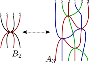
Figure 12. $A_{3}$ weave unfolding the 8-valent vertex for $B_{2}$

In fact, there are two possible weaves here related by Zamolodchikov relation [14, Section 4.2.6], and we can choose either one. Let us analyze the behaviour of Lusztig cycles under unfolding. First, the variables $t_{i}$ from (11) transform in the weave as follows:

$$\left(t^{a},t^{a},t^{b},t^{c},t^{c},t^{d}\right)\to\left(t^{a},\frac{t^{b}t^{c}}{t^{a}+t^{c}},t^{a}+t^{c},\frac{t^{a}t^{b}}{t^{a}+t^{c}},t^{c},t^{d}\right)\to$$

$$\left(t^{a},\frac{t^{b}t^{c}}{t^{a}+t^{c}},t^{a}+t^{c},\frac{t^{c}t^{d}(t^{a}+t^{c})}{\pi_{1}},\frac{\pi_{1}}{t^{a}+t^{c}},\frac{t^{a}t^{b}t^{c}}{\pi_{1}}\right)\to\left(t^{a},\frac{t^{b}t^{c}}{t^{a}+t^{c}},\frac{t^{c}t^{d}(t^{a}+t^{c})}{\pi_{1}},t^{a}+t^{c},\frac{\pi_{1}}{t^{a}+t^{c}},\frac{t^{a}t^{b}t^{c}}{\pi_{1}}\right)\to$$

$$\left(\frac{t^{b}t^{2c}t^{d}\pi_{1}}{\pi_{2}},\frac{\pi_{2}}{\pi_{1}},\frac{t^{a}t^{b}t^{c}\pi_{1}}{(t^{a}+t^{c})\pi_{2}},t^{a}+t^{c},\frac{\pi_{1}}{t^{a}+t^{c}},\frac{t^{a}t^{b}t^{c}}{\pi_{1}}\right)\to$$

$$\left(\frac{t^{b}t^{2c}t^{d}}{\pi_{2}},\frac{\pi_{2}}{\pi_{1}},\frac{\pi_{2}}{\pi_{1}},\frac{\pi_{1}^{2}}{\pi_{2}},\frac{t^{a}t^{b}t^{c}}{\pi_{1}},\frac{t^{a}t^{b}t^{c}}{\pi_{1}}\right).$$

Here we have used the notation

$$\pi_{1}:=t^{a}t^{b}+(t^{a}+t^{c})t^{d},\quad\pi_{2}:=t^{2a}t^{b}+(t^{a}+t^{c})^{2}t^{d}$$

and employed the identities

$$t^{a}\pi_{1}+t^{c}t^{d}(t^{a}+t^{c})=\pi_{2},\quad t^{a}t^{b}t^{c}+\pi_{2}=(t^{a}+t^{c})\pi_{1}.$$

Note that the weights for the edges colored by $1$ and $3$ agree both in the input and the output. By tropicalizing, we get precisely the equation (25). Similarly, any $B_{2}$ weave $\mathfrak{W}$ can be “unfolded” to an $A_{3}$ weave $\mathfrak{W}^{\prime}$ which has the following symmetry:

Lemma 6.3.

Let $\mathfrak{W}^{\prime\prime}$ be an $A_{3}$ weave obtained from $\mathfrak{W}^{\prime}$ by swapping the colors for $1$ and $3$. Then $\mathfrak{W}^{\prime\prime}$ is equivalent to $\mathfrak{W}^{\prime}$ with added 4-valent vertices at the top and at the bottom.

Proof.

This is a local check, so it is sufficient to check it for trivalent and 8-valent vertices in the $B_{2}$ weave $\mathfrak{W}$. A $2$-colored trivalent vertex in $\mathfrak{W}$ lifts to a 2-colored trivalent vertex in $\mathfrak{W}^{\prime}$ or $\mathfrak{W}^{\prime\prime}$, so there is nothing to check. A $1$-colored trivalent vertex in $\mathfrak{W}$ to a pair of $1$- and $3$-colored trivalent vertices in $\mathfrak{W}^{\prime}$, these are swapped in $\mathfrak{W}^{\prime\prime}$. Since we can move a $3$-colored strand through a $1$-colored trivalent vertex, and a $1$-colored strand through a $3$-colored trivalent vertex, we get the desired equivalence. Finally, an 8-valent vertex in $\mathfrak{W}$ lifts to a weave in Figure 12 with reduced braid words on top and bottom, and any two such weaves are equivalent. ∎

By abusing notations, one can say that there is a $\mathbb{Z}_{2}$ action on the weave $\mathfrak{W}^{\prime}$ which sends it to $\mathfrak{W}^{\prime\prime}$ and adds 4-valent vertices at the top and at the bottom. We can summarize the properties of braid varieties and weaves under unfolding as follows:

Proposition 6.4.

Let $\beta$ be a braid word for $B_{2}$, and $\beta^{\prime}$ its unfolding to $A_{3}$ where we replace each $\sigma_{1}$ in $\beta$ (assume there are $n_{1}$ of these) by $\sigma_{1}\sigma_{3}$ in $\beta^{\prime}$. Then the following holds:

• The group $H=(\mathbb{Z}_{2})^{n_{1}}$ acts on $X(\beta^{\prime})$ by swapping each $\sigma_{1}$ and $\sigma_{3}$, and swapping the corresponding $z$-variables.

• The fixed point locus $X(\beta^{\prime})^{H}$ is isomorphic to $X(\beta)$. Furthermore, the fixed point locus for the diagonal $\mathbb{Z}_{2}\subset H$ coincides with $X(\beta)$ as well.

• Any $B_{2}$ weave $\mathfrak{W}$ for $\beta$ can be unfolded to an $A_{3}$ weave $\mathfrak{W}^{\prime}$ for $\beta^{\prime}$, and the action of $\mathbb{Z}_{2}$ extends to $\mathfrak{W}^{\prime}$ as in Lemma 6.3.

• $B_{2}$ cycles lift to either one $\mathbb{Z}_{2}$-invariant cycle, or two $A_{3}$ cycles exchanged by the action of $\mathbb{Z}_{2}$.

• To calculate the entry $\varepsilon_{v,v^{\prime}}$ of the exchange matrix for two trivalent vertices $v$ and $v^{\prime}$ of $\mathfrak{W}$, one takes the intersection between the average of lifts of $\gamma_{v}$ and the sum of lifts of $\gamma_{v^{\prime}}$ in $\mathfrak{W}^{\prime}$. In this sense it is just a restriction of the $A_{3}$ intersection form/Poisson structure.

Proof.

Parts (1)-(2) are clear, (3) is a straightforward consequence of Lemma 6.3, and (4) is clear.

To prove (5), suppose that $\gamma_{v}$ and $\gamma_{v^{\prime}}$ lift to $k$ and $k^{\prime}$ cycles with total sums $\widetilde{\gamma_{v}}$ and $\widetilde{\gamma_{v^{\prime}}}$ respectively. Let $\eta$ be an arbitrary slice of $\mathfrak{W}$ and $\eta^{\prime}$ the corresponding slice of $\mathfrak{W}^{\prime}$. We claim that

$$\sharp_{\eta}(\gamma^{\vee}_{v}\cdot\gamma_{v^{\prime}})=\frac{1}{k}\sharp_{\eta^{\prime}}\left(\widetilde{\gamma_{v}}\cdot\widetilde{\gamma_{v^{\prime}}}\right).$$

To lighten the notation, we will denote $C:=\gamma_{v}$, $C^{\vee}:=\gamma_{v}^{\vee}$ and $C^{\prime}:=\gamma_{v^{\prime}}$. First we make some simple observations. Suppose that $\rho_{i}$ is a root associated to an edge in some slice. This edge has some color which is then associated with a simple root $\alpha$. By definition, $\rho_{i}$ is a Weyl group translate of $\alpha$. Edges with color $\alpha$ lift to $\langle\alpha^{\vee},\alpha^{\vee}\rangle$ roots after unfolding, where we normalize the pairing $\langle-,-\rangle$ so that if $\rho^{\vee}$ is a short coroot, then $\langle\rho^{\vee},\rho^{\vee}\rangle=1$. Thus an edge labelled by $\rho_{i}$ lifts to $\langle\rho_{i}^{\vee},\rho_{i}^{\vee}\rangle$ roots after unfolding.

Now suppose that a root $\rho_{i}$ lifts to $a=\langle\rho_{i}^{\vee},\rho_{i}^{\vee}\rangle$ roots $\widetilde{\rho}_{i,1},\ldots\widetilde{\rho}_{i,a}$ with the same weight $c_{i}$ in the unfolding, while a coroot $\rho_{j}^{\vee}$ lifts to $b=\langle\rho_{j}^{\vee},\rho_{j}^{\vee}\rangle$ coroots $\widetilde{\rho}_{j,1}^{\vee},\ldots\widetilde{\rho}_{j,b}^{\vee}$ with the same weight $c^{\prime}_{i}$ in the unfolding.

We need a few facts:

• $c_{i}^{\vee}=\frac{\langle\rho_{i}^{\vee},\rho_{i}^{\vee}\rangle}{k}c_{i}$, this is Lemma 6.1.

• $\widetilde{\rho}_{i,1},\ldots\widetilde{\rho}_{i,a}$ are mutually orthogonal, so that $(\widetilde{\rho}_{i,x},\widetilde{\rho}^{\vee}_{i,y})=0$ unless $x=y$.

• $(\rho_{i},\rho_{j}^{\vee})=(\widetilde{\rho}_{i,x},\sum_{t=1}^{b}\widetilde{\rho}_{j,t}^{\vee})$ for any lift $\widetilde{\rho}_{i,x}$ of $\rho_{i}$.

We are now ready to calculate

$$c_{i}^{\vee}c^{\prime}_{j}(\rho_{i},\rho^{\vee}_{j})=c_{i}^{\vee}c^{\prime}_{j}\left(\widetilde{\rho}_{i,1},~{}\sum_{t=1}^{b}\widetilde{\rho}_{j,t}^{\vee}\right)=\frac{a}{k}c_{i}c^{\prime}_{j}\left(\widetilde{\rho}_{i,1},~{}\sum_{t=1}^{b}\widetilde{\rho}_{j,t}^{\vee}\right)=\frac{1}{k}c_{i}c^{\prime}_{j}\left(\sum_{t=1}^{a}\widetilde{\rho}_{i,t},~{}\sum_{t=1}^{b}\widetilde{\rho}_{j,t}^{\vee}\right).$$

Hence the boundary intersections of $(C^{\vee},C^{\prime})$ and $(\widetilde{C},\widetilde{C^{\prime}})$ differ by a factor of $k$. Therefore the intersections at any $(2d_{ij})$-valent vertex differ by a factor $k$ as well, and the result follows. ∎

More generally, we can unfold any non simply-laced Dynkin diagram: $C_{n}$ unfolds to $A_{2n-1}$, $B_{n}$ unfolds to $D_{n+1}$, $G_{2}$ unfolds to $D_{4}$ and $F_{4}$ unfolds to $E_{6}$. Proposition 6.4 and its proof have a straightforward generalization to all these cases. We define a diagonal matrix $D:=\operatorname{diag}(d_{v})$ using Formula (24).

Lemma 6.5.

The matrix $\varepsilon D^{-1}$ is skew-symmetric, so $\varepsilon$ is skew-symmetrizable.

Proof.

Suppose that trivalent vertices $v,v^{\prime}$ unfold to $d_{v}$ and $d_{v^{\prime}}$ trivalent vertices, respectively. Let $\gamma_{v},\gamma_{v^{\prime}}$ be the corresponding cycles, and let $\widetilde{\gamma_{v}},\widetilde{\gamma_{v^{\prime}}}$ be the sum of all of their respective lifts. Then by Proposition 6.4(5) we get

$$\varepsilon_{v,v^{\prime}}=\frac{1}{d_{v}}\left(\widetilde{\gamma_{v}},\widetilde{\gamma_{v^{\prime}}}\right),\quad\varepsilon_{v^{\prime},v}=\frac{1}{d_{v^{\prime}}}\left(\widetilde{\gamma_{v^{\prime}}},\widetilde{\gamma_{v}}\right),$$

so $\varepsilon_{v,v^{\prime}}d_{v^{\prime}}^{-1}=-\varepsilon_{v^{\prime},v}d_{v}^{-1}$ and the result follows. ∎

6.3. Weave equivalence

We would like to relate different weaves by weave equivalences and mutations. The definition of weave mutation is unchanged, but the definition of weave equivalence is modified similarly to the 2-color relation in Soergel calculus [22], see below. There is one such equivalence relation (generalizing 1212 from Figure 4) for each rank 2 subdiagram, see Figure 13. Informally, one can say that the weave equivalence allows one to push a trivalent vertex through a braid relation.

Figure 13. Weave equivalences for $B_{2}$ (left) and $G_{2}$ (right) from braid word graphs

Proposition 6.6.

In any type, the weave equivalence does not change the $\varepsilon$-matrix, the intersection form and the cluster variables.

Proof.

If a weave has no trivalent vertices inside, the intersection form can be computed using Lemma 4.25 and, in particular, does not depend on the choice of braid relations for the fixed input and output.

Next, we need to check the equivalence relations in rank 2. In types $A_{2}$ and $A_{1}\times A_{1}$ this is done above. In type $B_{2}$, we unfold the 8-valent vertex to an $A_{3}$ weave as in Figure 12. For the weave equivalence, we have two cases: either we add a trivalent vertex labeled by 2, or we add a trivalent vertex labeled by 1 for $B_{2}$ which unfolds to a pair of trivalent vertices labeled by 1 and 3 for $A_{3}$. In the first case, after unfolding we get an $A_{3}$ weave with one trivalent vertex. By Theorem 4.4 any two such weaves are related by a sequence of (type $A$) weave equivalences and mutations. Since there is only one trivalent vertex, there are no mutations. In the second case, we have two trivalent vertices, but the corresponding type $A$ quiver has two frozen and no mutable vertices, so there are no mutations either.

Therefore by Lemma 4.27 and Lemma 5.2 the cluster variables and the intersections between cycles in the unfolded weave do not change, hence they do not change for the $B_{2}$ weave as well. ∎

6.4. Double inductive weaves

We would like to encode ways of writing $\beta$ by adding letters on the left and on the right. This is reminiscent of the double-reduced words of Berenstein, Fomin and Zelevinsky [2]. We will notate such a way of writing $\beta$ by a double string of entries of the form $iX$ where $i$ is the number of a node in the Dynkin diagram, and $X=L$ or $R$. The entry $iX$ means that we should add the braid letter $\sigma_{i}$ on the left if $X=L$ and on the right if $X=R$. For example, $(2L,1R,3R,1L,2L,2R)$ encodes writing the positive braid word $\sigma_{2}\sigma_{1}\sigma_{2}\sigma_{1}\sigma_{3}\sigma_{2}$ using the following string of subwords: $\underline{\sigma_{2}}$, $\sigma_{2}\underline{\sigma_{1}}$, $\sigma_{2}\sigma_{1}\underline{\sigma_{3}}$, $\underline{\sigma_{1}}\sigma_{2}\sigma_{1}\sigma_{3}$, $\underline{\sigma_{2}}\sigma_{1}\sigma_{2}\sigma_{1}\sigma_{3}$, $\sigma_{2}\sigma_{1}\sigma_{2}\sigma_{1}\sigma_{3}\underline{\sigma_{2}}$.

Suppose that we can write $\beta$ using the double string $(i_{1}X_{1},i_{2}X_{2},\dots,i_{l}X_{l})$. Let us call $\beta_{k}$ the $k$-th subword (of length $k$) coming from a double string. We may set $\beta_{0}=e$, the identity. Then $\beta_{k+1}=\sigma_{i_{k+1}}\beta_{k}$ or $\beta_{k}\sigma_{i_{k+1}}$ depending on whether $X_{k+1}=L$ or $R$, respectively.

Let us now construct the weave associated to a double string, that we call a double inductive weave. At each stage we get a weave from $\beta_{k}$ to $u_{k}:=\delta(\beta_{k})$. We start with the empty weave. If $\ell(u_{k+1})=\ell(u_{k})+1$, then we just add a strand of color $i_{k+1}$ on the left or right, depending on whether $X_{k+1}=L$ or $R$. Otherwise, we have $\ell(u_{k+1})=\ell(u_{k})$. In this case, we add a strand of color $i_{k+1}$ on the left or right, and this strand can form a trivalent vertex with an additional strand of color $i_{k+1}$. In both cases, we see that we get a weave from $\beta_{k+1}$ to $u_{k+1}=\delta(\beta_{k+1})$. For example, the left inductive weave $\overleftarrow{\mathfrak{w}}(\beta)$ is the weave associated to $(i_{r}L,i_{r-1}L,\dots,i_{1}L)$, while the right inductive weave $\overrightarrow{\mathfrak{w}}(\beta)$ is associated to $(i_{1}R,i_{2}R,\dots,i_{r}R)$.

Note that in the first entry in the double string, the $L$ or $R$ is superfluous, and does not affect the resulting string of subwords or the corresponding weave. We will sometimes suppress $X_{1}$ or freely change it between $L$ and $R$.

We will often abbreviate the first $k$ entries in the double string by $\beta_{k}$ if we are not concerned with this part of the double string. For example, we might write a double string as $(\beta_{k},i_{k+1}X_{k+1},i_{k+2}X_{k+2},\dots)$. It will be convenient to introduce a book-keeping device into our notation. Given a double string $(i_{1}X_{1},i_{2}X_{2},\dots,i_{l}X_{l})$, let us write the $(k+1)$-st entry as $i_{k+1}X_{k+1}^{+}$ when $\ell(u_{k+1})=\ell(u_{k})+1$. In other words, we will add a superscript “+” to those entries that increase the length of the Demazure product. For example, if we are working in type $A_{4}$, the word $(2L,1R,3R,1L,2L,2R)$ would be written $(2L^{+},1R^{+},3R^{+},1L^{+},2L,2R^{+})$.

Remark 6.7.

Note that, given a double string for $\beta$, $(i_{1}X_{1},i_{2}X_{2},\dots)$ where $X_{i}\in\{R,L\}$, the cluster variables for the braid variety $X(\beta)$ are in correspondence with the steps that do not increase the length of the Demazure product, that is, with the complement of those entries that have a $+$ in the superscript. Theorem 5.6(3) is valid for the double inductive weaves, with the same proof.

Theorem 6.8.

Let $\mathfrak{W}_{1}$ and $\mathfrak{W}_{2}$ be double inductive weaves for the braid word $\beta$ in arbitrary type. Then, $\mathfrak{W}_{1}$ and $\mathfrak{W}_{2}$ are related by a sequence of weave equivalences and mutations.

Proof.

We will consider the following kinds of moves on double strings:

$$(i_{1}L,i_{2}X_{2},\dots)\longleftrightarrow(i_{1}R,i_{2}X_{2},\dots)$$

$$(\beta_{k},iL,jR,\dots)\longleftrightarrow(\beta_{k},jR,iL,\dots)$$

First, observe that any two double strings for the same braid word $\beta$ are related by a series of the two moves above. The first move is trivial, as remarked before, and does not change the weave. The second move breaks down into several cases. We will break up the cases according to the lengths of $\ell(s_{i}*u_{k})$, $\ell(u_{k}*s_{j})$ and $\ell(u_{k+2})$, which we will now analyze.

1. Case 1: $(\beta_{k},iL^{+},jR^{+},\dots)\longleftrightarrow(\beta_{k},jR^{+},iL^{+},\dots)$

   First, let us suppose that $\ell(s_{i}*u_{k})=\ell(u_{k})+1$, $\ell(u_{k}*s_{j})=\ell(u_{k})+1$ and $\ell(u_{k+2})=\ell(u_{k})+2$. Both weaves come from just adding an $i$ strand on the left and a $j$ strand on the right. Thus, the weave does not change, the cluster variables do not change, and the cluster variables are still attached to the same entries.
   

2. Case 2: $(\beta_{k},iL^{+},jR,\dots)\longleftrightarrow(\beta_{k},jR^{+},iL,\dots)$

   This is the case where $\ell(s_{i}*u_{k})=\ell(u_{k})+1$ and $\ell(u_{k}*s_{j})=\ell(u_{k})+1$, but $\ell(u_{k+2})=\ell(u_{k})+1$.

   We have that

   $$u_{k+2} =s_{i}*u_{k}*s_{j}$$

   $$=s_{i}*u_{k}$$

   $$=s_{i}u_{k}$$

   $$=u_{k}*s_{j}$$

   $$=u_{k}s_{j}.$$

   From this, we get that $s_{i}u_{k}=u_{k}s_{j}$. Because $\ell(u_{k})<\ell(u_{k}s_{j})$, we know that $u_{k}$ cannot be written with an $s_{j}$ on the right. However, $s_{i}u_{k}$ can be written with an $s_{j}$ on the right. This means that this $s_{j}$ must come from moving $s_{i}$ to the right through $u_{k}$ using a series of braid moves. Similarly, moving $s_{j}$ to the left through $u_{k}$ using a series of braid moves gives an $s_{i}$ on the left.
   

   Let us now compare the weaves coming from the two different double strings: The weave for $(\beta_{k},iL^{+},jR,\dots)$ comes from adding an $i$ strand on the left, pulling it through $u_{k}$ using braid moves, and then merging with the $j$ strand on the right to get a trivalent vertex. The weave for $(\beta_{k},jR^{+},iL,\dots)$ comes from adding an $j$ strand on the right, pulling it through $u_{k}$ using braid moves, and then merging with the $i$ strand on the left to get a trivalent vertex. These two weaves are related by a series of equivalences, see Figure 14 below.
   

   Thus we have that the weaves are equivalent. The cluster variables stay the same, but the cluster variable attached to the entry $jR$ in $(\beta_{k},iL^{+},jR,\dots)$ becomes the cluster variable attached to the entry $iL$ in $(\beta_{k},jR^{+},iL,\dots)$.

   An important specialization of this is when $u_{k}=w_{0}$. Under this specialization, we will have that $j=i^{*}$. This situation will arise repeatedly in Section 10, when we compare our work with previous work on cluster structures on Richardson varieties.

   

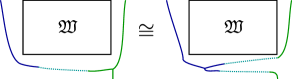
   Figure 14. On the left, the weave for the double sequence $(\beta_{k},iL^{+},jR)$. On the right, the weave for $(\beta_{k},jR^{+},iR)$. These weaves are equivalent.

3. Case 3: $(\beta_{k},iL^{+},jR,\dots)\longleftrightarrow(\beta_{k},jR,iL^{+},\dots)$

   This is the unique case where $\ell(s_{i}*u_{k})=\ell(u_{k})+1$ and $\ell(u_{k}*s_{j})=\ell(u_{k})$. In this case we must have that $\ell(u_{k+2})=\ell(s_{i}*u_{k}*s_{j})=\ell(u_{k})+1$.
   

   In this case, because adding $j$ to the right of $\beta_{k}$ results in a trivalent vertex, one can write a reduced word for $u_{k}$ with an $s_{j}$ on the right. This means that the trivalent vertex coming from adding $j$ on the right does not interact with adding a strand $i$ on the left. Thus, the weave does not change, the cluster variables do not change, and the cluster variables are still attached to the same entries.
   

   There is a similar case with the roles of $L$ and $R$ reversed, which can be treated similarly.
   

4. Case 4: $(\beta_{k},iL,jR,\dots)\longleftrightarrow(\beta_{k},jR,iL,\dots)$ and $\ell(s_{i}u_{k}s_{j})=\ell(u_{k})-2$.

   Cases 4 and 5 will deal with what happens when $\ell(s_{i}*u_{k})=\ell(u_{k})$ and $\ell(u_{k}*s_{j})=\ell(u_{k})$. In both these cases, we have that $\ell(s_{i}u_{k})=\ell(u_{k})-1$ and $\ell(u_{k}s_{j})=\ell(u_{k})-1$. Therefore we have that $\ell(s_{i}u_{k}s_{j})=\ell(u_{k})$ or $\ell(u_{k})-2$. We deal with the latter case first.
   

   If $\ell(s_{i}u_{k}s_{j})=\ell(u_{k})-2$ means that $u_{k}$ has a reduced expression of the form $s_{i}\cdots s_{j}$. Thus adding an $i$ strand on the left and a $j$ strand on the right gives trivalent $i$ vertex on the left and a trivalent $j$ vertex on the right. These trivalent vertices do not interact with each other. Thus the resulting double inductive weave are identical, the cluster variables are the same, and they remain attached to the same entries.
   

5. Case 5:$(\beta_{k},iL,jR,\dots)\longleftrightarrow(\beta_{k},jR,iL,\dots)$ and $\ell(s_{i}u_{k}s_{j})=\ell(u_{k})$.

   In this case, we have that $u_{k}=s_{i}v$ for some reduced word $v$ of length one less than $u_{k}$. Note that $v$ cannot be written with $s_{j}$ at the end. Thus $\ell(vs_{j})=\ell(v)+1=\ell(u_{k})$. Let $\gamma$ be the lift of $v$ to the braid group. From this, we have that $\ell(s_{i}*u_{k}*s_{j})=\ell(u_{k}*s_{j})$. This means that $u_{k}=\delta(s_{i}*u_{k}*s_{j})=\delta(u_{k}*s_{j})$. Therefore we have $u_{k}=vs_{j}$. This means that when we write $u_{k}$ with the strand $i$ on the left, and in order to use braid moves to write it with strand $j$ on the right, we have to pull the $i$ strand through $v$ to get the $j$ strand on the left.
   

   Now we can compare the weaves on the two sides. The weave for $(\beta_{k},iL,jR,\dots)$ comes from writing $u_{k}$ with an $i$ strand on the left. We add another $i$ strand and create a trivalent vertex. The $i$ strand on this trivalent vertex then gets pulled to the right using braid moves until it becomes a $j$ strand on the right, which merges with the $j$ strand added on the right to give another trivalent vertex, see Figure 15 below.
   

   There are two cluster variables. The first variable, which is attached to $iL$, has a cycle starting at the left $i$ trivalent vertex and ending on the right $j$ trivalent vertex. The second cluster variable, which is attached to $jR$, starts at the right $j$ trivalent vertex and goes downwards.
   

   Mutation at the cycle corresponding to the first variable gives precisely the weave corresponding to $(\beta_{k},jR,iL,\dots)$. The cluster variable formerly attached to $iL$ mutates to become the one attached to $jR$. The variable formerly attahced to $jR$ does not change, but it is now labelled by $iL$.
   

   This case has some similarities to Case 2, with the role of $u_{k}$ in Case 2 now played by $v$. An important specialization of Case 5 is when $u_{k}=w_{0}$. Under this specialization we will again have that $j=i^{*}$. This situation will also arise repeatedly in Section 10.

   

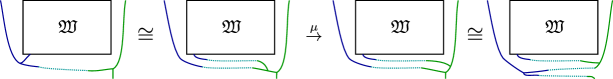
   Figure 15. On the left, the weave for the double sequence $(\beta_{k},iL,jR,\dots)$. On the right, the weave for $(\beta_{k},jR,iL,\dots)$. These weaves are related by a mutation.

In summary, Cases 1, 3 and 4 are uninteresting. The moves

$$(\beta_{k},iL^{+},jR^{+},\dots)\longleftrightarrow(\beta_{k},jR^{+},iL^{+},\dots)$$

$$(\beta_{k},iL^{+},jR,\dots)\longleftrightarrow(\beta_{k},jR,iL^{+},\dots)$$

$$(\beta_{k},iL,jR,\dots)\longleftrightarrow(\beta_{k},jR,iL,\dots)\textrm{ and }\ell(s_{i}u_{k}s_{j})=\ell(u_{k})-2$$

involve no changes in either cluster variables or which entry corresponds to which cluster variable.

Case 2 is mildly interesting in that the move

$$(\beta_{k},iL^{+},jR,\dots)\longleftrightarrow(\beta_{k},jR^{+},iL,\dots)$$

changes the entry corresponding to the unique cluster variable, though the weave is unchanged.

Case 5 is the only move involving a mutation. In the move

$$(\beta_{k},iL,jR,\dots)\longleftrightarrow(\beta_{k},jR,iL,\dots)\textrm{ and }\ell(s_{i}u_{k}s_{j})=\ell(u_{k}),$$

the cluster variable attached to $iL$ on the left mutates to the cluster variable attached to $jR$ on the right, while the cluster variable attached to $jR$ on the right does not change but becomes labelled by the cluster variable attached to $iL$ on the right. ∎

Corollary 6.9.

In arbitrary type, the cluster seeds associated to any two double inductive weaves are mutation equivalent.

Proof.

The proofs of Lemma 4.30 and Lemma 5.3 still apply, so weave mutations correspond to the mutations of the exchange matrix and cluster variables. By Proposition 6.6, weave equivalences do not change the exchange matrix or cluster variables. Now the result follows from Theorem 6.8. ∎

6.5. Cluster structures in the non simply-laced case

With these results and notations, we are ready to prove Theorem 1.1 in the non-simply laced case for double inductive weaves.

Theorem 6.10.

Let $\mathsf{G}$ be a simple algebraic group, $\beta\in\operatorname{Br}_{W}^{+}$ a positive braid word and $\mathfrak{w}:\beta\to\delta(\beta)$ a double inductive weave. Then we have

$$\mathbb{C}[X(\beta)]\cong\mathrm{up}(\varepsilon_{\mathfrak{w}})=\mathcal{A}(\varepsilon_{\mathfrak{w}}),$$

where $\varepsilon_{\mathfrak{w}}$ is the skew-symmetrizable exchange matrix associated to $\mathfrak{w}$ in Section 6.1.

Proof.

The proof follows the argument for the simply laced case, as presented in Section 5, quite closely. Thus we only list the key steps and necessary changes:

• Since we are considering double inductive weaves, where Theorem 6.8 and Corollary 6.9 apply, the cluster seeds associated to the left and right inductive weaves are mutation equivalent.

• In the case of Bott-Samelson varieties, the results of Section 4.8 in the simply-laced case imply the corresponding results (for Bott-Samelson varities) in the non-simply laced case, as follows. Assume the Dynkin diagram $\mathsf{D}$ is obtained from $\mathsf{D}^{\prime}$ via folding. Note that the unfolding of the longest word in $W(\mathsf{D})$ is the longest word in $W(\mathsf{D}^{\prime})$. Thus, a braid of the form $\Delta\beta\in\operatorname{Br}(\mathsf{D})$ unfolds to $\Delta^{\prime}\beta^{\prime}\in\operatorname{Br}(\mathsf{D}^{\prime})$. As for the weaves, except possibly for $4$-valent vertices that do not influence the exchange matrix, the inductive weave $\overrightarrow{\mathfrak{w}}(\Delta\beta)$ unfolds to $\overrightarrow{\mathfrak{w}}(\Delta^{\prime}\beta^{\prime})$; this follows from Remark 4.6. The result now follows since the exchange matrix $B$ for $\operatorname{Conf}(\beta)$ is obtained from that of $\operatorname{Conf}(\beta^{\prime})$ via folding, see e.g. [24, Section 3.6]. The results of Section 5.2 go through in the non-simply laced case with the same proofs. Thus, at this point we can conclude that Theorem 1.1 is true in the non-simply laced case for words of the form $\Delta\beta$.

• The freezing argument from Lemma 5.14 remains unchanged and applies in the non-simply laced case, from which we conclude the equality $\mathbb{C}[X(\beta)]=\mathrm{up}(\varepsilon_{\mathfrak{w}})$ between the ring of functions and the upper cluster algebra.

• Finally, in order to prove that cyclic rotation is a quasi-cluster transformation, we use the corresponding statement of Theorem 5.17, which follows from the simply laced case by unfolding. Note that if the weave $\mathfrak{W}$ in Figure 11 is double inductive, then both $\mathfrak{W}_{1}$ and $\mathfrak{W}_{2}$ are double inductive as well. This proves that $\mathbb{C}[X(\beta)]\subseteq\mathcal{A}(\varepsilon_{\mathfrak{w}})$ and thus $\mathbb{C}[X(\beta)]=\mathcal{A}(\varepsilon_{\mathfrak{w}})$.

∎

Theorem 6.10 constructs cluster structures in arbitrary type. The only difference with Theorem 1.1 is that the latter states that any Demazure weave can be used to construct a cluster seed, whereas the former restricts to double inductive weaves. Let us now conclude Theorem 1.1 by providing the following generalization of Lemma 4.4 in arbitrary type.

Proposition 6.11.

Let $\mathfrak{W}_{1},\mathfrak{W}_{2}:\beta\to\delta(\beta)$ be Demazure weaves in arbitrary type, where we have fixed a braid word for $\delta(\beta)$. Then $\mathfrak{W}_{1}$ and $\mathfrak{W}_{2}$ are related by a sequence of weave equivalences and mutations.

Proof.

We follow the logic of [21] and [14, Section 4]. It is sufficient to check all possible overlaps of the braid relations and Demazure moves $ii\to i$ and verify the statement for all Demazure weaves in these cases. It is proven in [21, Lemma 5.1], in the language of minimal sets of ambiguities, that checking these overlaps is indeed sufficient in Type A and analogous arguments should apply for other types. Equivalently, we can draw the braid word graphs in all these cases and interpret the Demazure weaves as paths from top to bottom vertex. We need to check that, up to mutations, all cycles in these graphs are generated by pentagons as in Figure 13 and squares (for non-overlapping moves).

The overlap between two Demazure moves is a mutation. The overlap between a Demazure move and a braid relation (for example, $11212$ in type $B_{2}$) is covered by Figure 13. This leaves us with the overlaps between two braid relations. To check these, we can restrict to a rank 2 subdiagram and consider the braid word graphs for $\beta=1212\ldots$ with $\ell(\beta)=d+k,k\leq d-1$, where $d=d_{12}$ is the length of the braid relation.

We proceed by induction in $k$, the base case $k=1$ is our definition of equivalence, see Figure 13. Assume that we verified the statement for all $\beta=1212\ldots$ with $\ell(\beta)\leq d+k-1$, then we verified all overlaps of lengths at most $d+k-1$ and by the above argument any two weaves for an arbitrary braid word of length at most $d+k-1$ are equivalent.

Now consider $\beta=1212\ldots$ with $\ell(\beta)=d+k,k\leq d-1$. We can apply $(k+1)$ different braid relations to $\beta$ and obtain braid words $\beta^{\prime}_{a},1\leq a\leq k+1$. Note that $\ell(\beta^{\prime}_{a})=d+k$. It is easy to see that our assumption $k\leq d-1$ implies that we cannot apply any braid relations to $\beta^{\prime}_{a}$ (except going back to $\beta$), so we must cancel double letters in all possible ways and obtain words $\beta^{\prime\prime}_{b},1\leq b\leq 2k$ of length $\ell(\beta^{\prime\prime}_{b})=d+k-1$. Specifically, $\beta^{\prime}_{1}$ is $\beta^{\prime\prime}_{1}=\underbrace{2121...}_{d+k-1}$ with one repeated letter, $\beta^{\prime}_{k+1}$ is $\beta^{\prime\prime}_{2k}=\underbrace{1212...}_{d+k-1}$ with one repeated letter, and for $2\leq a\leq k$ the word $\beta^{\prime}_{a}$ is $\alpha=\underbrace{1212...}_{d+k-2}$ with two repeated letters, and can be simplified to two words $\beta^{\prime\prime}_{2a-2},\beta^{\prime\prime}_{2a-1}$ which can be further simplified to $\alpha$. We illustrate these words in Figure 16 for type $B_{2}$, $d=4$ and $k=3$.

Figure 16. Braid words for type $B_{2}$, $d=4$ and $k=3$: $\beta$ on top, $\beta^{\prime}_{a}$ and $\beta^{\prime\prime}_{b}$ on next two layers and $\alpha$ at the bottom.

Consider an arbitrary path of braid words from $\beta$ to $\delta(\beta)=w_{0}$, it must pass through $\beta^{\prime\prime}_{b}$ for some $b$. By the assumption of induction, any two paths from $\beta^{\prime\prime}_{b}$ are equivalent, so we can choose a path from $\beta^{\prime\prime}_{b}$ to $w_{0}$ by first going to $\alpha$, and then following an arbitrary path to $w_{0}$. On the other hand, we can describe all cycles involving $\beta,\beta^{\prime\prime}_{b}$ and $\alpha$: there are $k$ pentagons (weave equivalences), $k-1$ squares (non-overlapping relations), and $k-2$ triangles of the form:

Here we denote by $1^{*}$ the index of the conjugate of the generator $s_{1}$ by $w_{0},$ which is $1$ for even $d$ and $2$ for odd $d$. A straightforward verification shows that such a triangle can be obtained as a combination of three elementary equivalences (one of them corresponding to a commutative square in the braid word graph and two others corresponding to pentagons) and two mutations. Therefore, any two paths from $\beta$ to $\alpha$ are mutation equivalent, and any two paths from $\beta$ to $w_{0}$ are mutation equivalent. ∎

Theorem 6.10 and Proposition 6.11 now imply Theorem 1.1 in its entirety:

Corollary 6.12.

Let $\mathsf{G}$ be a simple algebraic group, $\beta\in\operatorname{Br}_{W}^{+}$ a positive braid word and $\mathfrak{w}:\beta\to\delta(\beta)$ a Demazure weave. Then we have

$$\mathbb{C}[X(\beta)]\cong\mathrm{up}(\varepsilon_{\mathfrak{w}})=\mathcal{A}(\varepsilon_{\mathfrak{w}}).$$

where $\varepsilon_{\mathfrak{w}}$ is the skew-symmetrizable exchange matrix associated to $\mathfrak{w}$.

6.6. Langlands dual seeds

Consider a Demazure weave $\mathfrak{w}:\beta\to\delta(\beta)$ for a simple algebraic group $\mathsf{G}$. This gives us a cluster seed for the braid variety $X(\beta)$. The Langlands dual group $\mathsf{G}^{\vee}$ has the same Weyl group and braid group. Therefore, $\mathfrak{w}$ can also be viewed as a weave $\beta\to\delta(\beta)$ for $\mathsf{G}^{\vee}$ and it also gives a seed for the corresponding braid variety for $\mathsf{G}^{\vee}$; let us refer to this variety $X^{\vee}(\beta)$. Let us study how the seeds for $X(\beta)$ and $X^{\vee}(\beta)$ obtained from $\mathfrak{w}$ are related to each other.

Definition 6.13 ([26]).

Two cluster seeds $(I,I^{\operatorname{uf}}\!,\varepsilon,d)$ and $(\tilde{I},\tilde{I}^{\operatorname{uf}}\!,\tilde{\varepsilon},\tilde{d})$ are said to be Langlands dual if there is a bijection between $I$ and $\tilde{I}$ inducing a bijection between $I^{\operatorname{uf}}$ and $\tilde{I}^{\operatorname{uf}}$ such that

• $\varepsilon_{ij}=-\tilde{\varepsilon}_{ji}$,

• $\tilde{d}_{i}=d_{i}^{-1}c$ for some constant $c$.

In other words, the exchange matrices are transposed and negated, while the multipliers are inverted up to rescaling.

Proposition 6.14.

Let $\mathfrak{W}$ be a weave for a braid word $\beta$. Then the corresponding seeds for the cluster varieties $X(\beta)$ and $X^{\vee}(\beta)$ are Langlands dual.

Proof.

Let $v$ and $v^{\prime}$ be trivalent vertices of $\mathfrak{W}$. Let $\varepsilon_{v,v^{\prime}}$ be the corresponding entry in the exchange matrix for $X(\beta)$, and $\varepsilon^{\vee}_{v,v^{\prime}}$ that for $X^{\vee}(\beta)$. We would like to check that $\varepsilon_{v,v^{\prime}}=-\varepsilon^{\vee}_{v,v^{\prime}}$.

This can be checked purely locally at trivalent vertices and at $(2d)$-valent vertices. In principle, this is a finite check that can just be done by hand, though it is somewhat tedious. We will give a conceptual proof for the most interesting case, the $(2d)$-valent vertices.

We use Equation 27 to conclude that for any slice $\eta$, we have

$$\sharp_{\eta}(\gamma^{\vee}_{v}\cdot\gamma_{v^{\prime}}):=\frac{1}{2}\sum_{i,j=1}^{r}\operatorname{sign}(j-i)c_{i}^{\vee}c^{\prime}_{j}\cdot(\rho_{i},\rho^{\vee}_{j})=-\frac{1}{2}\sum_{i,j=1}^{r}\operatorname{sign}(i-j)c^{\prime}_{j}c_{i}^{\vee}\cdot(\rho^{\vee}_{j},\rho_{i})=-\sharp_{\eta}(\gamma_{v^{\prime}}^{\vee}\cdot\gamma_{v}).$$

By taking $\eta$ to be a slice before and after any $(2d)$-valent vertex, we see that the local contribution to the intersection pairing at a vertex $\bar{v}$ satisfies

$$\sharp_{\bar{v}}(\gamma_{v}^{\vee}\cdot\gamma_{v^{\prime}})=-\sharp_{\bar{v}}(\gamma_{v^{\prime}}\cdot\gamma_{v}^{\vee}).$$

as needed.

Suppose that at a trivalent vertex $\bar{v}$, we have that $\gamma_{v}$ has weight $c$ along the left vertex and $\gamma_{v^{\prime}}$ has weight $c^{\prime}$ along the right vertex. Then

$$\sharp_{\bar{v}}(\gamma_{v^{\prime}}^{\vee}\cdot\gamma_{v})=-cc^{\prime}\frac{d_{\bar{v}}}{d_{v}}=-c^{\vee}c^{\prime},$$

so that again we have $\sharp_{\bar{v}}(\gamma_{v^{\prime}}^{\vee}\cdot\gamma_{v})=-\sharp_{\bar{v}}(\gamma_{v}\cdot\gamma_{v^{\prime}}^{\vee})$

Finally, it is easy to verify that the constant $c$ required by Definition 6.13 can be taken to be the square ratio between the length of a long root and that of a short root, so $c=2$ in types $BC$ and $F_{4}$, and $c=3$ in type $G_{2}$.

∎

Section 8 below shows that braid varieties admit a cluster Poisson structure. Moreover, under the conditions of Lemma 8.1 and the existence of a cluster DT-transformation, proven in Section 8, we can conclude that the braid varieties $X(\beta)$ and $X^{\vee}(\beta)$ are cluster dual.

7. Properties and further results

This section collects a series of properties and results about the weaves and cluster structures presented thus far. These are additional facts that are not required for any of the previous results but might still be of independent interest. Each of the following subsections is also logically independent of each other.

7.1. A characterization of frozen variables

In this subsection, we give a combinatorial characterization of the trivalent vertices of a weave $\mathfrak{W}$ whose associated cluster variable is frozen. We start with the following lemma, which is a consequence of Corollary 5.21 and [41, Theorem 2.2]:

Lemma 7.1.

Let $\mathfrak{W}:\beta\to\delta(\beta)$ be a weave and $v$ its trivalent vertex. Then, $v$ is frozen if and only if the cluster variable $A_{v}$ is nowhere vanishing on $X(\beta)$.

Lemma 7.1 allows us to give a characterization of frozen trivalent vertices of a weave $\mathfrak{W}$ that has the combinatorial advantage of not referencing the cycle $\gamma_{v}$, as follows. Let us suppose that a trivalent vertex $v$ of $\mathfrak{W}$ corresponds to a move

$$\beta^{\prime}=\beta_{1}\sigma_{i}\sigma_{i}\beta_{2}\to\beta_{1}\sigma_{i}\beta_{2}.$$

By definition, this trivalent vertex $v$ is said to be Demazure frozen if $\delta(\beta_{1}\beta_{2})<\delta(\beta^{\prime})=\delta(\beta)$. It is easy to see [14, Section 5.1] that, if $\tilde{z}$ denotes the variable on the right arm of the trivalent vertex $v$, then we have a decomposition of the form

$$X(\beta^{\prime})=(X(\beta_{1}\sigma_{i}\beta_{2})\times\mathbb{C}^{*})\sqcup(Y\times\mathbb{C})$$

for some algebraic variety $Y$, where the strata correspond to $\widetilde{z}\neq 0$ and $\widetilde{z}=0$ respectively. In particular, $v$ is Demazure frozen if and only if $Y$ is empty or, equivalently, the locus $\{\tilde{z}=0\}$ is empty.

Lemma 7.2.

Let $\mathfrak{W}$ be a weave and $v\in\mathfrak{W}$ a trivalent vertex. Then, $v$ is frozen if and only if $v$ is Demazure frozen.

Proof.

Let us assume first that $v$ is not frozen, that is, the locus $\{A_{v}\neq 0\}$ is nonempty. Now consider the collection of all vertices $v^{\prime}$ that appear above $v$ on the weave, so that

$$A_{v}=\widetilde{z}\prod_{v^{\prime}}A_{v^{\prime}}^{m_{v^{\prime}}}$$

for some nonnegative integers $m_{v^{\prime}}$, cf. (18). To check that $v$ is not Demazure frozen, it is enough to check that the locus $\{\widetilde{z}=0\}\cap\{\prod_{v^{\prime}}A_{v^{\prime}}\neq 0\}$ is nonempty or, equivalently, that $\{A_{v}=0\}\not\subseteq\{\prod_{v^{\prime}}A_{v^{\prime}}=0\}$. By assumption, $\{A_{v}\neq 0\}\neq\emptyset$ and by [41, Theorem 1.3] cluster variables are irreducible, so $A_{v}$ and $\prod_{v^{\prime}}A_{v^{\prime}}$ are coprime. Thus, $v$ is not Demazure frozen. Conversely, assume that $v$ is not Demazure frozen. We want to check that $\{A_{v}=0\}\neq\emptyset$. But by definition $v$ not being Demazure frozen means that the locus $\{\prod_{v^{\prime}}A_{v^{\prime}}\neq 0\}\cap\{\widetilde{z}=0\}$ is nonempty, and the result follows. ∎

Lemma 7.2 can be used to give an upper bound on the number of frozen vertices of the cluster structure on $\mathbb{C}[X(\beta)]$.

Proposition 7.3.

Let $\beta\in\operatorname{Br}_{W}^{+}$ be a positive braid and $\mathfrak{W}:\beta\to\delta(\beta)$ a Demazure weave. Then the cluster structure $\mathcal{A}(\varepsilon_{\mathfrak{W}})=\mathbb{C}[X(\beta)]$ has at most $\ell(\beta)$ frozen variables.

The upper bound in Proposition 7.3 is sharp. Indeed, there are braid words such that $Q_{\mathfrak{W}}$ has exactly $\ell(\delta(\beta))$ frozen variables. For example, take any reduced word $\delta$ and let $\boldsymbol{\delta}\in\operatorname{Br}_{W}^{+}$ be obtained by repeating every letter of $\delta$ at least twice; then the left inductive weave $\overleftarrow{\mathfrak{w}}(\boldsymbol{\delta})$ has a quiver $Q_{\overleftarrow{\mathfrak{w}}(\boldsymbol{\delta})}$ which is a disjoint union of $\ell(\delta)$ linearly-oriented type $A$ quivers, each with one frozen variable.

Let us show Proposition 7.3. The non-simply laced case is proven similarly to the simply laced case by unfolding, so we will focus on the latter. In order to prove Proposition 7.3 in the simply laced case, it is enough to show that the quiver $Q_{\overleftarrow{\mathfrak{w}}(\beta)}$ for the left inductive weave has at most $\ell(\delta(\beta))$ frozen vertices. For each trivalent vertex $v$ of $\overleftarrow{\mathfrak{w}}(\beta)$, we define a path $\iota(v)$ in the weave $\overleftarrow{\mathfrak{w}}(\beta)$ as follows:

1. Start at $v$ and move downwards from this trivalent vertex.

2. If we reach another trivalent vertex, say $v_{2}$, the path $\iota(v)$ stops at $v_{2}$.

3. If the path $\iota(v)$ enters a hexavalent vertex from the upper left (resp. upper right, resp. upper center) edge, then it exists the hexavalent vertex from the lower right (resp. lower left, resp. lower middle) edge.

4. If the path $\iota(v)$ enters a tetravalent vertex from the upper left (resp. upper right) edge, then it exists the tetravalent vertex from the lower right (resp. lower left) edge.

Note that $\iota(v)$ is, in general, different from the cycle $\gamma_{v}$. By definition, the trivalent vertex $v$ is said to fall down if $\iota(v)$ does not stop, i.e., if $\iota(v)$ never reaches a trivalent vertex. Since we can always trace back $\iota(v)$ to $v$, we have an injection from the set of trivalent vertices that fall down to the letters of (a reduced decomposition of) $\delta(\beta)$. Thus, Proposition 7.3 follows from the following result.

Lemma 7.4.

Let $v$ be a Demazure frozen trivalent vertex of the weave $\overleftarrow{\mathfrak{w}}(\beta)$. Then $v$ falls down.

Proof.

Note that if $v$ is a trivalent vertex in $\overleftarrow{\mathfrak{w}}(\beta)$, then the left arm of $v$ goes straight up to $\beta$, without encountering any vertices. From here, it follows easily that the right arm of $v$ cannot lead directly to the middle strand of a hexavalent vertex. In fact, more is true. Assume that we have taken a trivalent vertex $v$ in the weave $\overleftarrow{\mathfrak{w}}(\beta)$ and we have slided it up through tetra- and hexavalent vertices using moves from [14, 4.2.4]. We obtain a weave $\widetilde{\mathfrak{w}}:\beta\to\delta(\beta)$ with a special trivalent vertex $\widetilde{v}$ on it. Since all the weave moves are local, note that the part of the weave which is placed northeast of $\widetilde{v}$ is a weave of the form $\overleftarrow{\mathfrak{w}}(\widetilde{\beta})$ where $\widetilde{\beta}$ is a suffix of $\beta$. From here, it follows again that the right arm of $\widetilde{v}$ cannot directly lead to the middle strand of a hexavalent vertex.

If we have two consecutive trivalent vertices $\beta_{1}s_{i}s_{i}s_{i}\beta_{2}\to\beta_{1}s_{i}s_{i}\beta_{2}\to\beta_{1}s_{i}\beta_{2}$ then the top trivalent vertex is never Demazure frozen. Assume now that $v$ is a trivalent vertex that does not fall down, i.e., such that $\iota(v)$ stops at another trivalent vertex, say $v_{1}$. If $\iota(v)$ does not pass any hexavalent or tetravalent vertex, then by the observation at the beginning of this paragraph $v$ cannot be Demazure frozen. If it does, we slide $v_{1}$ through these hexavalent and tetravalent vertices to bring it next to $v$. These are all legal moves since, by the discussion above, we will never have to slide $v_{1}$ through the middle strand of a hexavalent vertex. Note that sliding $v_{1}$ does not affect the condition that defines $v$ being Demazure frozen. Thus, $v$ cannot be Demazure frozen. ∎

The converse of Lemma 7.4 does not hold: $v$ falling down in $\overleftarrow{\mathfrak{w}}(\beta)$ does not imply that $v$ is (Demazure) frozen. For example, in Figure 26 below, which becomes a left inductive weave after reflecting along a vertical line, the top trivalent vertex falls down but it is not frozen.

Remark 7.5.

Note that in Lemma 7.4 it is essential that we work with the inductive weave $\overleftarrow{\mathfrak{w}}(\beta)$. For example, in Figure 6, the topmost trivalent vertex is Demazure frozen but it does not fall down.

7.2. Polynomiality of cluster variables

Theorem 1.1 proves that the algebra $\mathbb{C}[X(\beta)]$ is a cluster algebra. In particular, we have defined cluster variables and shown that they satisfy the corresponding exchange relations. In this subsection, we show that there is a way to lift the cluster variables in $\mathbb{C}[X(\beta)]$ to polynomials in $\mathbb{C}[z_{1},\dots,z_{r}]$, where $\ell(\beta)=r$, in such a way that the exchange relations are still satisfied. Note that Corollary 3.7 yields a projection $\pi:\mathbb{C}[z_{1},\dots,z_{r}]\to\mathbb{C}[X(\beta)]$. More precisely, we prove the following result:

Theorem 7.6.

Let $\beta=\sigma_{i_{1}}\cdots\sigma_{i_{r}}\in\operatorname{Br}^{+}_{W}$ and consider the projection $\pi:\mathbb{C}[z_{1},\dots,z_{r}]\to\mathbb{C}[X(\beta)]$. Then, for each cluster variable $c\in\mathbb{C}[X(\beta)]$, there exists a polynomial $\tilde{c}\in\mathbb{C}[z_{1},\dots,z_{r}]$ such that:

• $\pi(\tilde{c})=c$.

• The polynomials $\tilde{c}$ satisfy the cluster exhange relations: i.e.  if $\mathbf{c}=\{c_{1},\dots,c_{s}\}$ and $\mathbf{c}^{\prime}=\{c^{\prime}_{1},\dots,c^{\prime}_{s}\}$ are clusters in $\mathbb{C}[X(\beta)]$ related by a mutation in $k$ then, in $\mathbb{C}[z_{1},\dots,z_{r}]$, we have:

  $$\tilde{c}_{k}\tilde{c}^{\prime}_{k}=\prod_{i}\tilde{c}_{i}^{[\varepsilon_{ki}]_{+}}+\prod_{i}\tilde{c}_{i}^{-[\varepsilon_{ki}]_{-}}.$$

First, let us observe that the non-simply laced case of Theorem 7.6 follows from the simply laced case since, by Proposition 6.4 the cluster variables in the non-simply laced case can be obtained from those in the simply laced case by restricting to a closed subset. Thus, we focus in the simply laced case and we start proving Theorem 7.6 in the case of $\operatorname{Conf}(\beta)=X(\Delta\beta)$. We denote by $w$’s the variables corresponding to $\Delta$, by $z_{1},\dots,z_{r}$ the variables corresponding to $\beta$ and recall that

$$\operatorname{Conf}(\beta)=\{(z_{1},\dots,z_{r})\mid B_{\beta}(z)\in\mathsf{B}_{-}\mathsf{B}\}.$$

According to [68], the frozen variables in $\mathbb{C}[\operatorname{Conf}(\beta)]$ are precisely $f_{i}:=\Delta_{\omega_{i}}B_{\beta}(z)$, where $\Delta_{\omega_{i}}$ are generalized principal minors as in [29, 40]. So we can take this as the definition of $\tilde{f}_{i}$:

$$\tilde{f}_{i}:=\Delta_{\omega_{i}}B_{\beta}(z)\in\mathbb{C}[z_{1},\dots,z_{r}]\subseteq\mathbb{C}[w_{1},\dots,w_{\ell(w_{0})},z_{1},\dots,z_{r}]$$

Moreover, according to [68], we have

$$\mathbb{C}[\operatorname{Conf}(\beta)]=\mathbb{C}[z_{1},\dots,z_{r}][\tilde{f}_{i}^{-1}\mid i\in\mathsf{D}]$$

so that

$$\mathbb{C}[w_{1},\dots,w_{\ell(w_{0})},z_{1},\dots,z_{r}][\tilde{f}_{i}^{-1}\mid i\in\mathsf{D}]=\mathbb{C}[w_{1},\dots,w_{\ell(w_{0})}]\otimes\mathbb{C}[\operatorname{Conf}(\beta)]=\mathbb{C}[w_{1},\dots,w_{\ell(w_{0})}]\otimes\mathbb{C}[X(\Delta\beta)]$$

and Theorem 7.6 for $X(\Delta\beta)$ follows if we show that cluster variables do not involve denominators in frozen variables. For this, the following lemma is useful.

Lemma 7.7.

Let $f(z)\in\mathbb{C}[\operatorname{Conf}(\beta)]$ be a cluster variable. Then $f(z)$ is a cluster variable of $\mathbb{C}[\operatorname{Conf}(\beta\sigma_{i})]$ for every $i\in\mathsf{D}$.

Proof.

First, let us assume that $f(z)$ belongs to a cluster associated to a weave $\mathfrak{w}$ of $\Delta\beta$. Extend this weave to a weave $\mathfrak{w}^{\prime}$ of $\Delta\beta\sigma_{i}$ by adding an $i$-colored trivalent vertex on the bottom right of the weave. This adds a new cluster variable, but does not change the cluster variables that appeared before.

In general, assume that $f(z)=\mu_{k_{1}}\mu_{k_{2}}\cdots\mu_{k_{\ell}}g(z)$, where $g(z)$ is a cluster variable in a cluster coming from a weave $\mathfrak{w}$ and $k_{1},\dots,k_{\ell}$ are mutable vertices of the quiver $Q_{\mathfrak{w}}$. From the weave $Q_{\mathfrak{w^{\prime}}}$ as above. It is easy to see, cf. Lemma 4.44 and Remark 4.45, that this will:

• Add a new frozen variable.

• Thaw some frozen variables of $Q_{\mathfrak{w}}$.

• Add new coefficients to the matrix $\varepsilon$, all of which involve only variables mentioned in the previous two bullet points.

In particular, mutable variables of $Q_{\mathfrak{w}}$ do not have new incident variables in $Q_{\mathfrak{w}^{\prime}}$. Since $k_{1},k_{2},\dots,k_{\ell}$ correspond to mutable variables of $Q_{\mathfrak{w}}$, this implies that the equality $f(z)=\mu_{k_{1}}\cdots\mu_{k_{\ell}}g(z)$ is also valid in $\mathbb{C}[\operatorname{Conf}(\beta)]$ and we are done. ∎

Proposition 7.8.

Let $f(z)\in\mathbb{C}[\operatorname{Conf}(\beta)]=\mathbb{C}[z_{1},\dots,z_{r}][f_{i}^{-1}\mid i\in\mathsf{D}]$ be a cluster variable. Write

$$f(z)=h(z)/g(z)$$

where $h(z),g(z)\in\mathbb{C}[z_{1},\dots,z_{r}]$ have no common factors, and $g(z)$ is a monomial in $f_{i}$’s. Then, $g(z)=1$.

Proof.

Let $i\in\mathsf{D}$. By Lemma 7.7, $f(z)$ is also a cluster variable in $\mathbb{C}[\operatorname{Conf}(\beta\sigma_{i})]$. It is clear from the construction of the frozen variables, see also the proof of Proposition 4.41, that $f_{i}(z)$ is a cluster variable in $\mathbb{C}[\operatorname{Conf}(\beta\sigma_{i})]$ which is no longer frozen. Thus, $f_{i}(z)$ cannot divide $g(z)$ in $\mathbb{C}[z_{1},\dots,z_{r+1}]$ or in $\mathbb{C}[z_{1},\dots,z_{r}]$. The result follows. ∎

Theorem 7.6 for $\Delta\beta$ is now a consequence of Proposition 7.8. Let us now move on to general braid varieties.

Proof of Theorem 7.6.

Following the same argument as in the proof of Lemma 7.7, every cluster variable of $X(\beta)$ is also a cluster variable in $X(\Delta\beta)$ and, moreover, the exchange relations do not change. So the result follows from the corresponding statement on $X(\Delta\beta)$. ∎

Theorem 7.6 has the following geometric corollary.

Corollary 7.9.

For every braid $\beta=\sigma_{i_{1}}\cdots\sigma_{i_{r}}$ there exists a principal open set $U\subseteq\mathbb{C}^{r}$ such that:

• The inclusion $\pi^{*}:X(\beta)\to\mathbb{C}^{r}$ factors through $U$.

• There is a projection $\iota^{*}:U\to X(\beta)$ with section $\pi^{*}$.

Proof.

Let $f_{1},\dots,f_{k}$ be the frozen variables in $X(\beta)$ and let $U:=\{\prod_{i=1}^{k}\tilde{f}_{i}\neq 0\}\subseteq\mathbb{C}^{r}$. By the starfish lemma, we have an embedding $\iota:\mathbb{C}[X(\beta)]\to\mathbb{C}[U]=\mathbb{C}[z_{1},\dots,z_{r}][\tilde{f}_{i}^{-1}]$ sending the cluster variable $c$ to $\tilde{c}$. Now it is straightforward to verify (1) and (2). ∎

We refer the reader to Section 11 below for several examples of cluster variables where it is straightforward to verify that the exchange relations are already valid in the polynomial algebra.

7.3. Local acyclicity and reddening sequences

The purpose of this subsection is to show that the cluster algebra $\mathbb{C}[X(\beta)]$ is always locally acylic, in the sense of [62], and that it always admits a reddening sequence [52].

Let us first quickly discuss reddening sequences. Indeed, Lemma 4.44 implies that the quivers we consider have reddening sequences as follows:

Proposition 7.10.

Let $\mathfrak{W}:\beta\to\delta(\beta)$ be a Demazure weave. Its corresponding exchange matrix admits a reddening sequence.

Proof.

By Theorem 4.31, it is enough to fix a weave $\mathfrak{W}:\beta\to\delta(\beta)$ and we fix the inductive weave $\overleftarrow{\mathfrak{w}}(\beta)$. By Corollary 4.42 together with [68, Section 4] (see also [11, Corollary 4.9]), $\overrightarrow{\mathfrak{w}}(\Delta\beta)$ admits a maximal green sequence. Since $\overleftarrow{\mathfrak{w}}(\Delta\beta)$ is mutation equivalent to $\overrightarrow{\mathfrak{w}}(\Delta\beta)$, [63, Corollary 3.2.2] implies that $\overleftarrow{\mathfrak{w}}(\Delta\beta)$ has a reddening sequence. By Lemma 4.44 and [63, Theorem 3.1.3], then so does $\overleftarrow{\mathfrak{w}}(\beta)$. ∎

Assume that the exchange matrix of a cluster seed has full rank and its mutable part has a reddening sequence. Then, by works [26, 46], the corresponding upper cluster algebra has a canonical basis of theta functions parameterized by the integral tropicalization of the dual cluster $\mathcal{X}$-variety. In the skew-symmetric case, the upper cluster algebra also has a generic basis parameterized by the same lattice [65]. See [52] for more details and references. Thus, Proposition 7.10 implies the following corollary, see also Theorem 8.8 below.

Corollary 7.11.

The upper cluster algebra structure on $\mathbb{C}[X(\beta)]$ defined via Demazure weaves has a canonical basis of theta functions parameterized by the lattice of integral tropical points of the dual cluster $\mathcal{X}$-variety. If $\mathsf{G}$ is simply-laced, it also has a generic basis parameterized by the same lattice.

Proof.

We only need to show that the exchange matrix has full rank. This follows from Corollary 8.5 below, which is independent of the intervening material. ∎

Remark 7.12.

In fact, one expects that there is a precise link, close to be an equivalence, between the existence of a reddening sequence, local acyclicity, and the isomorphism between the upper cluster algebra and the cluster algebra, see [61].

Let us now focus on local acyclicity; recall that locally acylic means that there exists a finite open cover

$$X(\beta)=\bigcup_{i=1}^{k}U_{i}$$

where each $U_{i}$ is a cluster variety such that the mutable part of its associated quiver does not have directed cycles. Clearly, to show that $X(\beta)$ is locally acyclic it is enough to provide such a decomposition such that each $U_{i}$ is itself a locally acyclic cluster variety.

Theorem 7.13.

For any positive braid word $\beta\in\operatorname{Br}_{W}^{+}$, the cluster structure on the braid variety $X(\beta)$ is locally acyclic.

Proof.

We focus on the simply-laced case, the proof in the non-simply laced case is similar. As usual, let $\delta:=\delta(\beta)$. We work by induction on $\ell(\beta)-\ell(\delta)$, which is the number of vertices on the quiver $Q_{\mathfrak{W}}$ for any weave $\mathfrak{W}:\beta\to\delta$. Since the quiver $Q_{\mathfrak{W}}$ always has at least one frozen vertex, the result is clear for $\ell(\beta)-\ell(\delta)\in\{0,1,2\}$.

In the general case, upon applying a cyclic rotation to $\beta$ we may assume that $\beta=\sigma_{i}\sigma_{i}\beta^{\prime}$ for some positive braid word $\beta^{\prime}\in\operatorname{Br}^{+}_{W}$. If $\delta=s_{i}\delta(\beta^{\prime})$ then it is clear that we have $X(\beta)=\mathbb{C}^{\times}\times X(\beta^{\prime})$, while $\ell(\beta^{\prime})-\ell(\delta(\beta)^{\prime})=\ell(\beta)-\ell(\delta)-1$ and we may use induction to conclude that $X(\beta)$ is locally acyclic. So we will assume that $\delta=\delta(\beta^{\prime})$. In this case, we may consider a weave $\mathfrak{W}:\beta\to\delta$ as in Figure 17.

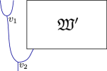
Figure 17. A weave $\mathfrak{W}:\sigma_{i}\sigma_{i}\beta^{\prime}\to\delta$, where $\mathfrak{W}^{\prime}$ is a weave $\mathfrak{W}^{\prime}:\beta\to\delta$. Note that $v_{1}\in Q_{\mathfrak{W}}$ is a mutable sink, while $v_{2}\in Q_{\mathfrak{W}}$ is a frozen source

.

Locally around $v_{1},v_{2}$ the quiver $Q_{\mathfrak{W}}$ looks as follows:

where $v^{\prime}_{1},\dots,v^{\prime}_{k}$ are the trivalent vertices $v$ such that $\gamma_{v}$ has a nonzero weight at the right incoming leg of $v_{2}$. We will consider the elements:

$$A_{1}:=A_{v_{1}},\qquad A_{2}:=\prod_{i=1}^{k}A_{v^{\prime}_{i}}$$

Mutating at $v_{1}$, we obtain that the element $\displaystyle{\frac{1+A_{v_{2}}A_{2}}{A_{1}}}$ is a regular function on $X(\beta)$ and therefore $A_{1}$ and $A_{2}$ cannot simultaneously vanish. In other words, $X(\beta)=U_{1}\cup U_{2}$, where $U_{i}=\operatorname{Spec}(\mathbb{C}[X(\beta)][A_{i}^{-1}])$. Let $Q_{1}$ be the quiver obtained from $Q_{\mathfrak{W}}$ by freezing the vertex $v_{1}$. We have (cf. [62, Proposition 3.1]):

$$\mathcal{A}(Q_{1})\subseteq\mathcal{A}(Q_{\mathfrak{W}})[A_{1}^{-1}]=\mathrm{up}(Q_{\mathfrak{W}})[A_{1}^{-1}]\subseteq\mathrm{up}(Q_{1}).$$

But $Q_{1}$ is easily seen to be a quiver for the braid word $\sigma_{i}\beta^{\prime}$ with a disjoint frozen vertex. By Corollary 5.21, $\mathcal{A}(Q_{1})=\mathrm{up}(Q_{1})$ and we conclude that $U_{1}=\operatorname{Spec}(\mathcal{A}(Q_{1}))=\mathbb{C}^{\times}\times X(\sigma_{i}\beta^{\prime})$ is a cluster variety that, by induction, is locally acyclic.

Similarly, let $Q_{2}$ be the quiver obtained from $Q_{\mathfrak{W}}$ by freezing the vertices $v^{\prime}_{1},\dots,v^{\prime}_{k}$, so that

$$\mathcal{A}(Q_{2})\subseteq\mathcal{A}(Q_{\mathfrak{W}})[A_{2}^{-1}]=\mathrm{up}(Q_{\mathfrak{W}})[A_{2}^{-1}]\subseteq\mathrm{up}(Q_{2}),$$

and $Q_{2}$ is easily seen to be the quiver $Q_{\mathfrak{W}^{\prime}}$ with a disjoint quiver of the form $\square\rightarrow\bullet$, so $\mathcal{A}(Q_{2})=\mathrm{up}(Q_{2})$ and $U_{2}=\operatorname{Spec}(\mathcal{A}(Q_{2}))=X(\beta^{\prime})\times X(\sigma_{i}^{3})$ which, again by induction, is locally acyclic. The result follows. ∎

A similar strategy to that of the proof of Theorem 7.13 allows us to deduce more properties on the quiver $Q_{\mathfrak{W}}$ and the variety $X(\beta)$. First, let us recall that the class $\mathcal{P}^{\prime}$ is the smallest class of quivers without frozen vertices that satisfies the following property:

• The quiver with a single vertex belongs to $\mathcal{P}^{\prime}$.

• If $Q\in\mathcal{P}^{\prime}$, then any quiver mutation equivalent to $Q^{\prime}$ also belongs to $\mathcal{P}^{\prime}$.

• If $Q\in\mathcal{P}^{\prime}$ and $Q^{\prime}$ is obtained from $Q$ by adjoining a sink or a source, then $Q^{\prime}\in\mathcal{P}^{\prime}$.

See [10, 11, 53]. We say that an iced quiver $Q$ belongs to $\mathcal{P}^{\prime}$ if its mutable part $Q^{\operatorname{uf}}$ belongs to $\mathcal{P}^{\prime}$.

Proposition 7.14.

For any braid $\beta\in\operatorname{Br}^{+}_{W}$ and any weave $\mathfrak{W}:\beta\to\delta$, the quiver $Q_{\mathfrak{W}}$ belongs to the class $\mathcal{P}^{\prime}$.

Proof.

Since cyclic rotation does not change the (mutation class of the) mutable part of the weave $\mathfrak{W}$, see Lemma 5.19, we may assume that $\beta$ has the form $\beta=\sigma_{i}\sigma_{i}\beta^{\prime}$ and take the weave $\mathfrak{W}$ as in Figure 17, so that $Q_{\mathfrak{W}}$ is obtained from $Q_{\mathfrak{W}^{\prime}}$ by adjoining a mutable sink and a frozen source and the result follows. ∎

Note that by [10, Theorem 3.3] this yields another (similar in spirit) proof of Proposition 7.10. By [53, Theorem 4.6], resp. by [64, Lemma 8.13], we also get the following corollaries.

Corollary 7.15.

For any braid $\beta\in\operatorname{Br}^{+}_{W}$ and any weave $\mathfrak{W}:\beta\to\delta$, the quiver $Q_{\mathfrak{W}}$ admits a unique non-degenerate potential (up to right equivalence). It is rigid and its Jacobian algebra is finite-dimensional.

Corollary 7.16.

For any braid $\beta\in\operatorname{Br}^{+}_{W}$ and any weave $\mathfrak{W}:\beta\to\delta$, any quantum cluster algebra whose exchange type is given by the quiver $Q_{\mathfrak{W}}$ equals its corresponding quantum upper cluster algebra.

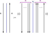
Figure 18. The topological 1-cycle near an $s_{i}$-edge of the weave and the shorthand notation of train tracks, where the number $a\in\mathbb{N}$ indicates $a$ parallel copies. The numbers $(i)$ in parentheses indicate that the segment in the plane parallel to an $s_{i}$-edge is lifted to the $i$th sheet of the branched cover. Note that the orientations are depicted.

7.4. Topological view on weave cycles

Let us provide a topological interpretation of weaves and their cycles, building on [18, Section 2]; for this subsection we set $\mathsf{G}=\operatorname{SL}_{n+1}$. Given a weave $\mathfrak{W}\subset\mathbb{R}^{2}$ with $n$ colors, $s_{1},\ldots,s_{n}\in S_{n+1}$, let $S(\mathfrak{W})$ be the smooth surface obtained as a simple $(n+1)$-fold branched cover of $\mathbb{R}^{2}$ along the trivalent vertices of $\mathfrak{W}$, where the monodromy transposition around a trivalent vertex is declared to be $s_{i}$ if the (three) edges incident to the vertex are labeled with $s_{i}\in S_{n}$. The weave $\mathfrak{W}$ itself can then be interpreted as branch cuts for the projection $S(\mathfrak{W})$ onto $\mathbb{R}^{2}$; there are more branch cuts than necessary but that is allowed and this choice appears naturally in this interpretation.

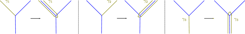
Figure 19. The projections to $\mathbb{R}^{2}$ of the relative 1-cycles $\gamma_{1},\gamma_{2},\gamma_{3}\subset S(\mathfrak{W}_{tri})$ near a trivalent vertex. Each cycle $\gamma_{i}$ has two projections, one contained in the weave $\mathfrak{W}_{tri}$ and the other is (the projection of) its generic perturbation.

First, at a generic horizontal slice of the weave $\mathfrak{W}$ a local 1-cycle on $S(\mathfrak{W})$ of weight $a$ is defined according to Figure 18, with $a$ parallel copies at each side of an $s_{i}$-edge, lifting to sheet $i$. Figure 18 also prescribes the orientations which are needed to compute signed intersections. Second, by construction, the cycles $\gamma_{1},\gamma_{2}$ and $\gamma_{3}$ in Figure 19 lift to homonymous geometric relative 1-cycles on the surface $S(\mathfrak{W}_{tri})$ associated to the weave $\mathfrak{W}_{tri}$ given by a trivalent vertex, which is a 2-disk. Figure 19 actually depicts two projections to $\mathbb{R}^{2}$ of these cycles $\gamma_{1},\gamma_{2},\gamma_{3}\in S(\mathfrak{W}_{tri})$: a non-generic projection, literally above a weave edge, and a generic projection. The former provides neater descriptions of 1-cycles in terms of the edges of the weave itself, and the later is useful for computing intersection numbers, see [18, Section 2] and [17, Section 3]. These two different projections of each $\gamma_{i}$ lift to (smoothly) isotopic, and thus homologous, 1-cycles. In the notation of Section 4.4, $\gamma_{1}$ (resp. $\gamma_{2},\gamma_{3}$) geometrically realizes the weave cycle that has weight $1$ (resp. $0,0$) on the top leftmost edge, has weight $0$ on the top rightmost edge (resp. $0,0$) and weight $0$ (resp. $0,1$) on the bottom edge. A weave cycle in $\mathfrak{W}_{tri}$ with arbitrary weights $(a,b,c)\in\mathbb{Z}^{3}$ can be realized geometrically be a linear combination of these $\gamma_{1},\gamma_{2},\gamma_{3}$: such relative 1-cycle $\gamma(a,b;c)$ can be drawn by taking $a$ disjoint copies of $\gamma_{1}$, $b$ disjoint copies of $\gamma_{2}$ and $c$ disjoint copies of $\gamma_{3}$, oriented appropriately according to signs.

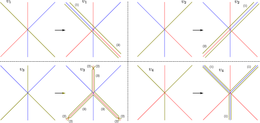
Figure 20. The projections to $\mathbb{R}^{2}$ of the relative 1-cycles $\upsilon_{1},\upsilon_{2},\upsilon_{3},\upsilon_{4}\subset S(\mathfrak{W}_{hex})$ near a hexavalent vertex. The numbers in parentheses indicate the sheet, $1,2$ or $3$, to which that part of the segment is being lifted. Note that adjustements at the ends of $\upsilon_{3}$ need to be inserted so as to have boundary conditions match with other pieces of the cycle according to the rule of Figure 18.

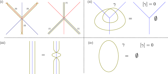
Figure 21. $(i)$ Two geometric relative 1-cycles associated to hexavalent vertices, in line with Figure 20. Parts $(ii),(iii)$ and $(iv)$ depict relations for the geometric 1-cycles that hold in the (relative) homology of $S(\mathfrak{W})$. The curve $\gamma$ in $(ii)$ is lifted to sheets $i$ and $i+1$ if the blue edges are $s_{i}$-edges; same with the curves in $(iii)$. The curve $\gamma$ in $(iv)$ is meant to be anywhere in $\mathbb{R}^{2}\setminus\mathfrak{W}$ and lifted to any sheet. In particular, both curves $\gamma$ in $(ii)$ and $(iv)$ are null-homologous in the first homology group $H_{1}(S(\mathfrak{W}),\mathbb{Z})$.

Third, Figure 20 similarly depicts cycles $\upsilon_{1},\upsilon_{2},\upsilon_{3},\upsilon_{4}$ that lift to (homonymous) geometric relative 1-cycles on the surface $S(\mathfrak{W}_{hex})$ associated to the weave $\mathfrak{W}_{hex}$ given by a hexavalent vertex, which consists of the (disjoint) union of three 2-disks. In the notation of Section 4.4, $\upsilon_{1}$ (resp. $\upsilon_{2},\upsilon_{3},\upsilon_{4}$) realizes the weave cycles with top weights $(1,0,0)$ (resp. $(0,0,1),(0,1,0),(1,0,1)$) and bottom weights $(0,0,1)$ (resp. $(1,0,0),(1,0,1),(0,1,0)$). Note that Figure 21.(i) also depicts the geometric cycles associated to those with top weights $(1,0,1)$, resp. $(0,1,0)$, and bottom weights $(0,1,0)$, resp. $(1,0,1)$, when the blue and red colors are exchanged. A weave cycle with arbitrary weights can be represented as a linear combination of these as well, which is geometrically represented by drawing copies of $\upsilon_{i}$ suitable superposed; denote this geometric 1-cycle by $\upsilon(a,b,c;a^{\prime},b^{\prime},c^{\prime})$. In both cases of $S(\mathfrak{W}_{tri})$ and $S(\mathfrak{W}_{hex})$, we refer to these actual relative 1-cycles as being geometric cycles, in contrast to the (algebraically defined) weave cycles in Definition 4.7. The following lemma states that the intersection numbers of these geometric cycles coincide with those intersection numbers defined in Section 4.4 for the respective weave cycles.

Lemma 7.17.

The algebraic intersections of the homology classes associated to the geometric 1-cycles in $S(\mathfrak{W}_{tri})$ and $S(\mathfrak{W}_{hex})$ described above coincide with the intersections of the corresponding weave cycles.

Proof.

This readily follows by computing the geometric intersections of the $\gamma_{i}$ and $\upsilon_{j}$ cycles among themselves. From the generic projections from Figure 19, it is immediate to see that the geometric intersection matrices are

$$(\langle\gamma_{i},\gamma_{j}\rangle)=\left(\begin{array}[]{ccc}0&-1&1\\ 1&0&-1\\ -1&1&0\\ \end{array}\right),\quad(\langle\upsilon_{i},\upsilon_{j}\rangle)=\left(\begin{array}[]{ccccc}0&-1&0&0\\ 1&0&0&0\\ 0&0&0&0\\ 0&0&0&0\end{array}\right),$$

and these coincide with the intersections from Section 4.4. ∎

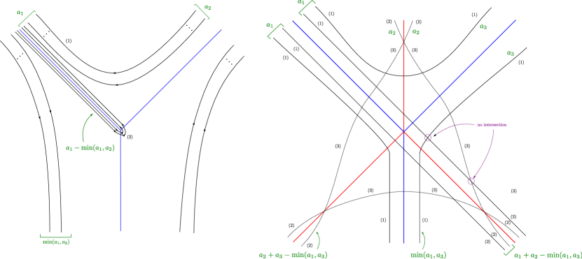
Figure 22. Embedded representative for the Lusztig cycles near a trivalent (left) and hexavalent vertices (right). The hexavalent picture uses the train track notation from Figure 18. In the hexavalent case, none of the intersections of the projection yield any geometric intersections in $S(\mathfrak{W}_{hex})$ as the branches near each intersection lift to different sheets. The trivalent picture is drawn in the case that $a_{2}<a_{1}$, the case $a_{1}<a_{2}$ is symmetric and the case $a_{1}=a_{2}$ would have no curves going near the trivalent vertex for $\mathfrak{W}_{tri}$. The hexavalent picture is drawn in the case that $a_{3}<a_{1}$, the case $a_{1}<a_{3}$ is also symmetric and the case $a_{1}=a_{3}$ would have no $\upsilon_{1}$-type curves going from the top left across to the bottom right.

In general, the geometric realizations $\gamma(a,b,c)\subset S(\mathfrak{W}_{tri})$ and $\upsilon(a,b,c;a^{\prime},b^{\prime},c^{\prime})\subset S(\mathfrak{W}_{hex})$ for arbitrary $a,b,c,a^{\prime},b^{\prime},c^{\prime}\in\mathbb{Z}$ described above are immersed relative 1-cycles. For Lusztig weave cycles, as in Definition 4.8, we can find embedded relative 1-cycles geometrically representing them, as follows:

Lemma 7.18.

Let $a_{1},a_{2},a_{3}\in\mathbb{Z}$ and . Then the relative 1-cycles $\gamma(a_{1},a_{2};\mbox{min}(a_{1},a_{2}))\subset S(\mathfrak{W}_{tri})$ and

$$\upsilon(a_{1},a_{2},a_{3};(a_{2}+a_{3}-\min(a_{1},a_{3}),\min(a_{1},a_{3}),a_{1}+a_{2}-\min(a_{1},a_{3}))\subset S(\mathfrak{W}_{hex}).$$

are represented in homology by the embedded relative 1-cycles in Figure 22.

Proof.

Let us describe the case of a trivalent vertex $\mathfrak{W}_{tri}$, the hexavalent case $\mathfrak{W}_{hex}$ is analogous. Consider the 1-cycle $\gamma(a_{1},a_{2};\mbox{min}(a_{1},a_{2}))\subset S(\mathfrak{W}_{tri})$, with its projection onto $\mathbb{R}^{2}$ as $a_{1}$ disjoint unions of $\gamma_{1}$ (the perturbed version), $a_{2}$ disjoint unions of $\gamma_{2}$ (the perturbed version) and $\mbox{min}(a_{1},a_{2})$ disjoint unions of $\gamma_{3}$, also the perturbed version. These can be drawn so that the geometric intersections between $a_{1}\cdot\gamma_{1}$ and $a_{2}\cdot\gamma_{2}$ lie in the upper triangle of $\mathbb{R}^{2}\setminus\mathfrak{W}_{tri}$, those between $a_{1}\cdot\gamma_{1}$ and $\mbox{min}(a_{1},a_{2})\cdot\gamma_{3}$ lie in the left triangle of $\mathbb{R}^{2}\setminus\mathfrak{W}_{tri}$, and those between $a_{2}\cdot\gamma_{2}$ and $\mbox{min}(a_{1},a_{2})\cdot\gamma_{3}$ lie in the right triangle of $\mathbb{R}^{2}\setminus\mathfrak{W}_{tri}$.

Consider the outmost copy of $\gamma_{1}$ and the outmost copy of $\gamma_{2}$ and surger their unique intersection point so that one of the components is a curve that stays in the top triangle, as the ones appearing at the top of Figure 22 (left). Iterate that procedure with the second outmost representatives, for a total of $\mbox{min}(a_{1},a_{2})$ times. Similarly, perform surgeries at the unique intersection of the outmost copy of $\gamma_{1}$ with the outmost copy of $\gamma_{3}$, and similarly for $\gamma_{2}$ and $\gamma_{3}$, and then iterate this procedure for a total of $\mbox{min}(a_{1},a_{2})$ times. The resulting 1-cycle geometrically represents $a_{1}\cdot\gamma_{1}+a_{2}\cdot\gamma_{2}+\mbox{min}(a_{1},a_{2})\cdot\gamma_{3}$. At this stage, the picture is that in Figure 22 (left) plus a collection of closed immersed curves each of which winds around the trivalent vertex twice. It suffices to notice that these are null-homologous cycles, as indicated in Figure 21.(ii), and thus Figure 22 (left) indeed represents this Lusztig cycle. ∎

We observe that computing intersections with these embedded representatives is rather immediate and yields the same results as in Section 4.4, see Figure 23. These local cycles from Figures 18 and 22 all glue globally to form geometric 1-cycles on $S(\mathfrak{W})$: at a generic horizontal slice of the weave $\mathfrak{W}$ the cycle continue according to Figure 18 and the boundary conditions match with those in Figure 22. For those Lusztig cycles that are contained in a compact region of $\mathfrak{W}$, the associated geometric 1-cycle is closed. For a Lusztig cycle that falls down, the associated geometric 1-cycle defines a relative 1-cycle. In general, these geometric 1-cycles can be simplified with the rules in Figure 21.$(ii)$, $(iii)$ and $(iv)$, plus other clear relations in homology, so as to obtain simpler representatives of their homology classes. For instance, a geometric 1-cycle might have several components, but if one of them is a curve $\gamma$ homologous to a curve as in Figure 21.$(ii)$ or $(iv)$, then that component $\gamma$ is null-homologous and can be erased.

Finally, there is substantial symplectic topology behind the theory of weaves, braid varieties and their cluster structures. The reader is referred to [13, 17, 18] for that symplectic geometric interpretation and its relation to the microlocal theory of sheaves, and to [16, Section 5] for its relation to Floer theory. In particular, see [17, Section 4] for a discussion of how certain first homology lattices associated to $S(\mathfrak{W})$ can arise as the natural $\mathcal{A}$- and $\mathcal{X}$-lattices.

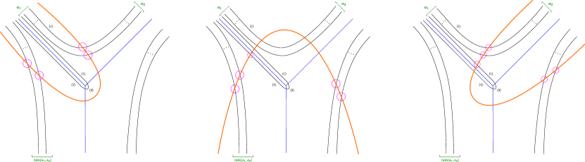
Figure 23. The intersections of $a_{1}\cdot\gamma_{1}+a_{2}\cdot\gamma_{2}+\mbox{min}(a_{1},a_{2})\cdot\gamma_{3}$ with $\gamma_{1}$, on the left, $\gamma_{2}$, on the right, and $\gamma_{3}$, center. Note that the intersections with $\gamma_{1}$ cancel.

8. Cluster Poisson structure

This section proves Corollary 1.3 and discusses DT-transformations.

8.1. Poisson structure

In this section, we prove that braid varieties admit not only a cluster $\mathcal{A}$-structure constructed in previous sections, but a cluster Poisson structure, also known as a cluster $\mathcal{X}$-structure. To start, we use the following fact:

Lemma 8.1.

Let $(\varepsilon_{ij})\in\mbox{Mat}(n,m)$, $n\leq m$ be the exchange matrix of a seed in a cluster algebra. Suppose we can find an integer square matrix $(p_{ij})\in\mbox{Mat}(m,m)$ such that the following two conditions are satisfied:

• $p_{ij}=\varepsilon_{ij}$, unless both $i$ and $j$ are frozen;

• $\mathrm{det}(p_{ij})=\pm 1$.

Then the collection $(X_{k}),k\in[m],$ together with the matrix $(p_{ij}),$ defines an initial seed of a cluster Poisson algebra, where $X_{k}$ are defined by the rule

(29) $$X_{k}=\prod A_{j}^{p_{kj}}.$$

By construction, $X_{k}$ are only rational functions on $X(\beta)$, whereas to $A_{k}$ being regular functions.

Proof.

The proof essentially follows from the calculations in [44, §18].

Let $\Lambda$ be a free $\mathbb{Z}$-module with a basis $\{f_{1},\ldots,f_{m}\}$. Let us set

$$e_{i}:=\sum_{j\in[m]}p_{ij}f_{j}.$$

Note that $\det(p_{ij})=\pm 1$. Therefore $\{e_{1},\ldots,e_{m}\}$ forms a new basis of $\Lambda$. Consider the algebraic torus $\mathcal{T}_{\Lambda}:={\rm Hom}(\Lambda,\mathbb{G}_{m})$. Each $v\in\Lambda$ corresponds to a character $T_{v}$ of $\mathcal{T}_{\Lambda}$. We set

$$X_{i}:=T_{e_{i}},\qquad A_{i}:=T_{f_{i}}.$$

The variables satisfy the relation (29).

Following Lemma 18.2 of [44], the mutation at $k\in[n]$ gives rise to a new unimodular matrix $(p_{ij}^{\prime})$ such that

(30) $$p_{ij}^{\prime}=\left\{\begin{array}[]{ll}-p_{ij}&\mbox{if $k=i$ or $k=j$}\\ p_{ij}+[p_{ik}]_{+}p_{kj}+p_{ik}[-p_{kj}]_{+}&\mbox{otherwise}.\end{array}\right.$$

Note that $p_{ij}^{\prime}=\varepsilon_{ij}^{\prime}$ unless both $i$ and $j$ are frozen. Recall that the cluster mutation $\mu_{k}$ gives rise to two new sets of variables $\{A_{i}^{\prime}\}$ and $\{X_{i}^{\prime}\}$ such that

$$A_{i}^{\prime}=\left\{\begin{array}[]{ll}A_{i}&\mbox{if }i\neq k\\ A_{k}^{-1}({\prod{A_{j}}^{[\varepsilon_{kj}]_{+}}+\prod A_{j}^{[-\varepsilon_{kj}]_{+}}})&\mbox{if }i=k.\end{array}\right.$$

$$X_{i}^{\prime}=\left\{\begin{array}[]{ll}X_{i}(1+X_{k}^{-{\rm sgn}(\varepsilon_{ik})})^{-\varepsilon_{ik}}&\mbox{if }i\neq k\\ X_{k}^{-1}&\mbox{if }i=k.\end{array}\right.$$

By Theorem 18.3 of [44], quantum versions of the above mutations are defined via conjugations with the quantum dilogarithm series following monomial changes. As a semi-classical limit, we obtain

(31) $$X_{i}^{\prime}:=\prod_{j}A_{j}^{\prime p_{ij}^{\prime}}.$$

In this way, we obtain a new algebraic torus with two sets of variables $\{A_{i}^{\prime}\}$ and $\{X_{i}^{\prime}\}$ related by (31).

Repeating the same procedure to the new obtained seeds/tori recursively, we obtain a cluster Poisson algebra (an upper cluster algebra resp.) as the intersection of the Laurent polynomial rings of the $X$ ($A$ resp.) variables. These two algebras are isomorphic locally via the isomorphism (29). ∎

Note that the existence of the matrix $(p_{ij})$ as in Lemma 8.1 implies that the (non-square) matrix $(\varepsilon_{ij})_{i\in I^{\operatorname{uf}},j\in I}$ has full rank.

Let us now perform the construction of Lemma 8.1 for the braid variety $X(\beta)$. Consider any Demazure weave $\mathfrak{W}:\beta\to\delta(\beta)$. We have defined a cluster algebra structure with a seed determined by $\mathfrak{W}$ on the algebra $\mathbb{C}[X(\beta)]$. Let $E$ be the set of edges on the southern boundary of $\mathfrak{W}$. The ordered sequence of edges $e\in E$ corresponds to a reduced decomposition of $w=\delta(\beta)$, which further gives rise to an ordered list of positive roots $\rho_{e}$ as in (14). Let $(\gamma_{i})$ be the collection of cycles corresponding to the trivalent vertices of $\mathfrak{W}$. Recall the bilinear form $(\cdot,\cdot)$ on the root lattice defined via (13). Following the notation of Lemma 8.1, we have the exchange matrix

$$\varepsilon_{ij}=\sum_{v\mbox{ vertex of }\mathfrak{W}}\#_{v}(\gamma^{\vee}_{i}\cdot\gamma_{j})+\frac{1}{2}\sum_{e,e^{\prime}\in E}{\rm sign}(e^{\prime}-e)\gamma_{i}^{\vee}(e)\gamma_{j}(e^{\prime})\left(\rho_{e},\rho^{\vee}_{e^{\prime}}\right).$$

where $i,j$ are trivalent vertices of the weave $\mathfrak{W}$. The second term corresponds to the boundary intersection number of $\gamma_{i}$ and $\gamma_{j}$ as in (27).

We now present a construction of a suitable matrix $(p_{ij})$ from a weave $\mathfrak{W}$. Set $\theta_{i}:=\theta_{i}(\mathfrak{W}),\theta_{i}^{\vee}:=\theta^{\vee}_{i}(\mathfrak{W})$ where

$$\theta_{i}(\mathfrak{W}):=\sum_{e\in E(\mathfrak{W})}\gamma_{i}^{\vee}(e)\rho_{e},\quad\theta^{\vee}_{i}(\mathfrak{W}):=\sum_{e\in E(\mathfrak{W})}\gamma_{i}(e)\rho^{\vee}_{e}.$$

Note that $\theta_{i},\theta_{i}^{\vee}\neq 0$ if and only if $i$ is frozen. We define $p_{ij}:=p_{ij}(\mathfrak{W})$ where

$$p_{ij}(\mathfrak{W}):=\varepsilon_{ij}-\frac{1}{2}\left(\theta_{i},\theta^{\vee}_{j}\right)=\varepsilon_{ij}-\frac{1}{2}\sum_{e,e^{\prime}\in E(\mathfrak{W})}\gamma_{i}^{\vee}(e)\gamma_{j}(e^{\prime})\left(\rho_{e},\rho^{\vee}_{e^{\prime}}\right).$$

Note that $p_{ij}=\varepsilon_{ij}$ unless both $i$ and $j$ are frozen, as required by Lemma 8.1.

Lemma 8.2.

For any Demazure weave, the matrix $(p_{ij})$ is an integer matrix.

Proof.

Note that

$$p_{ij} =\sum_{v\mbox{ vertex of }\mathfrak{W}}\#_{v}(\gamma^{\vee}_{i}\cdot\gamma_{j})+\sum_{e,e^{\prime}\in E}\frac{{\rm sign}(e^{\prime}-e)-1}{2}\gamma_{i}^{\vee}(e)\gamma_{j}(e^{\prime})\left(\rho_{e},\rho^{\vee}_{e^{\prime}}\right)$$

$$=\sum_{v\mbox{ vertex of }\mathfrak{W}}\#_{v}(\gamma^{\vee}_{i}\cdot\gamma_{j})-\sum_{e^{\prime}<e}\gamma_{i}^{\vee}(e)\gamma_{j}(e^{\prime})\left(\rho_{e},\rho^{\vee}_{e^{\prime}}\right)-\sum_{e\in E}\gamma_{i}^{\vee}(e)\gamma_{j}(e).$$

since $(\rho_{e},\rho^{\vee}_{e})=2$. It is clear that $p_{ij}$ is an integer by the last expression. ∎

Lemma 8.3.

The absolute value $|\det(p_{ij})|$ is independent of the Demazure weave $\mathfrak{W}$ chosen.

Proof.

It suffices to show that $|\det(p_{ij})|$ is invariant under the following three changes.

• Weave equivalences. The matrix $\varepsilon_{ij}$ and the vectors $\theta_{i},\theta_{i}^{\vee}$ remain invariant under weave equivalences. Hence $p_{ij}$ remains the same.

• Weave mutations. Note that the vectors $\theta_{i},\theta_{i}^{\vee}$ remain invariant under weave mutation. The matrix $\varepsilon_{ij}$ changes according to the mutation rule (1) for exchange matrices. Therefore the matrix $(p_{ij})$ changes as in (30). A direct check shows that $|\det(p_{ij})|$ is invariant.

• Add a $(2d_{ij})$-valent vertex at the bottom of the weave. It follows from Lemma 4.25 that the matrix $(\varepsilon_{ij})$ is invariant. Meanwhile a direct local check (and folding in non simply-laced case) shows that the vectors $\theta_{i},\theta_{i}^{\vee}$ are invariant as well. Therefore $(p_{ij})$ is invariant.∎

Lemma 8.4.

For any Demazure weave, $\mathrm{det}(p_{ij})=\pm 1$.

Proof.

We work by induction on $\ell(\beta)$, the case $\ell(\beta)=1$ is clear. So assume the result is true for $\beta$. If $\delta(\beta\sigma_{k})=\delta(\beta)s_{k}$ then $X(\beta\sigma_{k})=X(\beta)$ and there is nothing to do. Otherwise, we consider the following weave for $\beta\sigma_{k}$:

where we call $e$ the edge marked in yellow. The extra trivalent vertex corresponds to a cycle $\gamma_{m+1}$, with

$$\theta_{m+1}=-\delta(\beta)(\alpha_{k}),\quad\theta^{\vee}_{m+1}=-\delta(\beta)\left(\alpha^{\vee}_{k}\right).$$

Therefore

$$p_{i,m+1}=\gamma_{i}(e),\qquad p_{m+1,i}=-\gamma_{i}(e)-\left(\theta_{i},\theta_{m+1}^{\vee}\right),\qquad p_{m+1,m+1}=-1.$$

The matrix $p_{ij}$ for $\beta\sigma_{k}$ has the form:

$$\left(\begin{matrix}p_{11}&\cdots&p_{1m}&p_{1,m+1}\\ \vdots&\ddots&\vdots&\vdots\\ p_{m1}&\cdots&p_{mm}&p_{m,m+1}\\ p_{m+1,1}&\cdots&p_{m+1,m}&-1\end{matrix}\right)\longrightarrow\left(\begin{matrix}p^{\prime}_{11}&\cdots&p^{\prime}_{1m}&p_{1,m+1}\\ \vdots&\ddots&\vdots&\vdots\\ p^{\prime}_{m1}&\cdots&p^{\prime}_{mm}&p_{m,m+1}\\ 0&\cdots&0&-1\end{matrix}\right)$$

where the arrow means that we apply elementary matrix transformations, and

$$p^{\prime}_{ij} =p_{ij}+p_{i,m+1}p_{m+1,j}$$

$$=\varepsilon_{ij}-\frac{1}{2}(\theta_{i},\theta_{j}^{\vee})-\gamma^{\vee}_{i}(e)\gamma_{j}(e)-\gamma^{\vee}_{i}(e)(\theta_{j},\theta^{\vee}_{m+1})$$

$$=\left(\varepsilon_{ij}+\frac{1}{2}(\theta_{i},\theta_{m+1}^{\vee})\gamma_{j}(e)-\frac{1}{2}(\theta_{j},\theta^{\vee}_{m+1})\gamma^{\vee}_{i}(e)\right)-\frac{1}{2}\left(\theta_{i}+\gamma_{i}^{\vee}(e)\theta_{m+1},\theta_{j}^{\vee}+\gamma_{j}(e)\theta_{m+1}^{\vee}\right)$$

$$=\varepsilon_{ij}^{\prime}-\frac{1}{2}\left(\theta_{i}^{\prime},(\theta_{j}^{\prime})^{\vee}\right)$$

coincides with the matrix for the weave $\mathfrak{W}:\beta\to\delta(\beta)$. The result now follows by induction. ∎

Recall that an exchange matrix is said to be of full rank if the rectangular matrix $(\varepsilon_{ij}:i\ \mathrm{mutable},j\ \mathrm{arbitrary})$ has maximal rank equal to $|I^{\operatorname{uf}}|$, the number of mutable variables.

Corollary 8.5.

The exchange matrix $\varepsilon_{\mathfrak{W}}$ has full rank.

Proof.

If $i$ is mutable then $\varepsilon_{ij}=p_{ij}$, so the rectangular matrix $(\varepsilon_{ij}:i\ \mathrm{mutable},j\ \mathrm{arbitrary})$ consists of several rows of the matrix $p=(p_{ij})$. By Lemma 8.4 $p$ has maximal rank, and the result follows. ∎

Theorem 8.6.

The braid variety $X(\beta)$ admits a cluster Poisson structure.

Proof.

This follows from Lemma 8.4 combined with Lemma 8.1 ∎

8.2. DT transformation

Thanks to Proposition 7.10, together with the fact that the exchange matrix has maximal rank, the cluster Poisson variety $X(\beta)$ admits a Donaldson-Thomas (DT) transformation $\operatorname{DT}:X(\beta)\to X(\beta)$. In [68, Section 4] an explicit geometric realization for the DT-transformation is presented for (double) Bott-Samelson varieties; this is used in [17, Section 5] for a geometric description of the DT-transformation for grid plabic graphs of shuffle type. The goal of this section is to exhibit the DT-transformation explicitly for all braid varieties.

Let $\beta=\sigma_{i_{1}}\cdots\sigma_{i_{\ell}}$. Recall that we have the cyclic rotation

$$\rho:X(\beta)\to X(\sigma_{i_{\ell}^{*}}\sigma_{i_{1}}\cdots\sigma_{i_{\ell-1}})$$

that is a quasi-cluster transformation by Theorem 5.17. Applying this transformation $\ell(\beta)$ times we obtain $\rho^{\ell}:X(\beta)\to X(\beta^{*})$, where $\beta^{*}=\sigma_{i_{1}^{*}}\cdots\sigma_{i_{\ell}^{*}}$. On the other hand, since the map $i\mapsto i^{*}$ is an automorphism of the Dynkin diagram $\mathsf{D}$, there is a group automorphism $*:\mathsf{G}\to\mathsf{G}$, $x\mapsto x^{*}$, satisfying $\mathsf{B}^{*}=\mathsf{B}$, and $x\mathsf{B}\buildrel s_{i}\over{\longrightarrow}y\mathsf{B}$ if and only if $x^{*}\mathsf{B}\buildrel s_{i^{*}}\over{\longrightarrow}y^{*}\mathsf{B}$. It follows that we have an isomorphism of varieties

$$*:X(\beta)\to X(\beta^{*}).$$

It is easy to see that this is an isomorphism of cluster varieties, as follows. Let $\mathfrak{W}:\beta\to\delta(\beta)$ be a weave. From the description of the cluster torus $T_{\mathfrak{W}}\subseteq X(\beta)$ in terms of distances of flags, it is easy to see that $T^{*}_{\mathfrak{W}}\subseteq X(\beta^{*})$ is the cluster torus $T_{\mathfrak{W}^{*}}$, where $\mathfrak{W}^{*}:\beta^{*}\to\delta(\beta^{*})$ is obtained by changing the color of every strand while keeping the shape of the weave intact. Obviously, the quivers $Q_{\mathfrak{W}}$ and $Q_{\mathfrak{W}^{*}}$ agree. The fact that the cluster variables also agree follows since these are defined in terms of distances of framed flags.

As a slight modification and generalization of [29, Section 1.5], we define the twist automorphism:

$$D_{\beta}:=*\circ\rho^{\ell}:X(\beta)\to X(\beta).$$

Theorem 8.7.

The twist automorphism $D_{\beta}:X(\beta)\to X(\beta)$ is the $\operatorname{DT}$ transformation.

Proof.

As we have seen, the map $D_{\beta}$ is a quasi-cluster automorphism. It remains to show that, if $\mathfrak{W}:\beta\to\delta(\beta)$ is a weave and $D_{\beta}\mathfrak{W}:\beta\to\delta(\beta)$ a weave such that $D^{*}_{\beta}(T_{D_{\beta}\mathfrak{W}})=T_{\mathfrak{W}}$, then the mutable parts of $Q_{\mathfrak{W}}$ and of $Q_{T_{D_{\beta}}\mathfrak{W}}$ are related by a reddening sequence of mutations. By [62, Theorem 3.2.1], or [43, Theorem 3.6], it is enough to do this for a single weave.

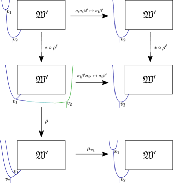
Figure 24. The weave $\mathfrak{W}$ for $\sigma_{i}\sigma_{i}\beta^{\prime}$ (upper left) and that for $\sigma_{i}\beta^{\prime}$ (upper right). The dotted arrows mean that we apply a cluster automorphism followed by a sequence of mutations. In the right dotted arrow, this sequence of mutations is a reddening sequence by inductive assumption.

We work by induction on $\ell(\beta)-\ell(\delta)$, the case $\ell(\beta)-\ell(\delta)\in\{0,1\}$ is clear. Let us assume for the time being that $\beta=\sigma_{i}\sigma_{i}\beta^{\prime}$ for some positive braid word $\beta^{\prime}$, where $\ell(\beta)=\ell+1$. If $\delta(\beta)=s_{i}\delta(\beta^{\prime})$ then we can reduce to the word $\beta^{\prime}$ as in the proof of Theorem 7.13, so we assume that $\delta(\beta)=\delta(\beta^{\prime})$. In this case, we may consider a weave $\mathfrak{W}$ as in the upper left corner of Figure 17. Following the notation of that figure, the cycle corresponding to $v_{1}$ is a mutable sink and the cycle corresponding to $v_{2}$ a frozen source. By the inductive assumption, the DT transformation for $\sigma_{i}\beta^{\prime}$ is $*\circ\rho^{\ell}$. We can apply the same transformation to $\beta$ to obtain the word $\sigma_{i}\beta^{\prime}\sigma_{i^{*}}$. Note that the quiver for $X(\sigma_{i}\beta)$ is a subquiver of that for $X(\sigma_{i}\beta\sigma_{i^{*}})$, so we can apply a reddening sequence of mutations for $X(\sigma_{i}\beta)$ to $X(\sigma_{i}\beta\sigma_{i^{*}})$, see Figure 24.

Applying another cyclic shift to $\sigma_{i}\beta^{\prime}\sigma_{i^{*}}$ we get a weave for $\beta=\sigma_{i}\sigma_{i}\beta^{\prime}$ that is related to the starting weave by mutation at the sink $v_{1}$. This is a reddening sequence for the quiver that consists of the single vertex $v_{1}$. Since $v_{1}$ is a sink, it follows from Lemma 2.3 in [10] that we have a reddening sequence for $Q_{\mathfrak{W}}$, so $\rho\circ*\circ\rho^{\ell}$ is the $\operatorname{DT}$ transformation for $\beta$. Now the result follows by observing that $\rho\circ*=*\circ\rho$.

In the general case, if $\ell(\beta)-\ell(\delta)>0$ we can apply a sequence $\tau$ of braid moves (that can be interpreted as cluster automorphisms) and cyclic shifts (that are quasi-cluster automorphisms) to bring $\beta$ to the form $\sigma_{i}\sigma_{i}\beta^{\prime}$. The diagram

commutes and it follows that $D_{\beta}$ is indeed the DT transformation of $X(\beta)$. ∎

Thanks to Theorems 1.1 and 8.6, the braid variety $X(\beta)$ admits both a cluster $\mathcal{A}$- and a cluster $\mathcal{X}$-structure. Moreover, Proposition 6.14 together with [26][Lemma 1.11] shows that, for any positive braid $\beta$, the pair $(X(\beta),X^{\vee}(\beta))$ is a cluster ensemble. Finally, since the exchange matrices have full rank (Corollary 8.5) and the braid varieties admit a DT transformation, results of [46] and [65] allow us to conclude the following result, which is an enhancement of Corollary 7.11.

Theorem 8.8.

Let $\beta$ be a positive braid. Then the pair $(X(\beta),X^{\vee}(\beta))$ is a cluster ensemble such that the Fock-Goncharov cluster duality conjecture holds. In particular, $\mathbb{C}[X(\beta)]$ admits a canonical basis of theta functions naturally parameterized by the integral tropicalization of the dual braid variety $X^{\vee}(\beta)$. If $\mathsf{G}$ is simply-laced, $\mathbb{C}[X(\beta)]$ also admits a generic basis parameterized by the same lattice.

9. Gekhtman-Shapiro-Vainshtein form

Since the cluster algebra $\mathbb{C}[X(\beta)]$ is locally acyclic, the canonical cluster $2$-form defined on the union of cluster tori extends to $X(\beta)$, see [62, Theorem 4.4]. The form on $X(\beta)$ is known as the Gekhtman-Shapiro-Vainshtein (GSV) form. In this section, we show that this GSV form may be constructed using the Maurer-Cartan form on the group $\mathsf{G}$ and the matrices $B_{\beta}$, similarly to [59] and [14, Section 3].

9.1. Construction of the form $\omega_{\beta}$ on $X(\beta)$

The construction of the 2-form $\omega_{\beta}$ on the braid variety $X(\beta)$ following Mellit [59], see also [14, Section 3]), is as follows. Throughout this section, we assume without loss of generality that $\delta(\beta)=w_{0}$, cf. Lemma 3.4. Let $\theta$, resp. $\theta^{R}$, denote the left (resp. right) invariant $\mathfrak{g}$-valued form on $\mathsf{G}$, also known as the Maurer-Cartan form, and $\kappa:\mathfrak{g}\otimes\mathfrak{g}\to\mathbb{C}$ the Killing form on the Lie algebra $\mathfrak{g}$ of $\mathsf{G}$. These define a $2$-form on $\mathsf{G}\times\mathsf{G}$ by:

$$(f|g):=\kappa(\theta(f)\wedge\theta^{R}(g))$$

The 2-form $(f|g)$ satisfies the following “cocycle condition”:

(32) $$(f|g)+(fg|h)=(f|gh)+(g|h).$$

Given a collection of $G$–valued functions $f_{1},\ldots,f_{\ell}$, we define

(33) $$(f_{1}|\cdots|f_{\ell}):=(f_{1}|f_{2})+(f_{1}f_{2}|f_{3})+\ldots+(f_{1}\cdots f_{\ell-1}|f_{\ell}).$$

By (32) this definition is associative in $f_{i}$. Using (33), we define the 2-form $\omega_{\beta}$ on $X(\beta)$ for $\beta=\sigma_{i_{1}}\cdots\sigma_{i_{\ell}}$ to be the restriction of the form

$$\omega:=(B_{i_{1}}(z_{1})|\cdots|B_{i_{\ell}}(z_{\ell}))\in\Omega^{2}(\mathbb{C}^{\ell})$$

to the braid variety $X(\beta)$. By definition, upon applying the map $B_{\beta}:\mathbb{C}^{\ell}\to\mathsf{G}$, the braid variety has its image contained in $w_{0}\mathsf{B}$. Thus, similarly to [14, Lemma 3.1], the restriction $\omega_{\beta}:=\omega|_{X(\beta)}$ yields a closed 2-form on $X(\beta)$.

Remark 9.1.

In case $\mathsf{G}=\operatorname{SL}_{n}$, we have $\theta(f)=f^{-1}df$ and $\theta^{R}(g)=dgg^{-1}$. Moreover, if $\Upsilon:\mathsf{G}_{1}\to\mathsf{G}_{2}$ is a homomorphism of Lie groups then $\Upsilon^{*}(\theta_{\mathsf{G}_{2}})=\theta_{\mathsf{G}_{1}}$; similarly for the right-handed versions. We use these facts below, together with pinnings (Section 3.4) to reduce several calculations to the $\operatorname{SL}$-case.

9.2. Coincidence of the forms

Let us show that the closed $2$-form $\omega_{\beta}$ coincides with the GSV form on $X(\beta)$. We proceed via several lemmas studying the restrictions of the form to braid words of length $2$ and $3$, where we may assume we work in the $\operatorname{SL}$-case, see Remark 9.1 above.

Lemma 9.2.

Suppose that $f=B_{i}(z)\chi_{i}(u)$. Then

• The pullback of the left-invariant one-form along $f$ equals

  $$f^{-1}df=\varphi_{i}\left(\begin{matrix}u^{-1}du&0\\ -u^{2}dz&-u^{-1}du\\ \end{matrix}\right)$$

• The pullback of the right-invariant one-form along $f$ equals

  $$df\cdot f^{-1}=\varphi_{i}\left(\begin{matrix}-u^{-1}du&dz+2u^{-1}zdu\\ 0&u^{-1}du\\ \end{matrix}\right)$$

Proof.

We have

$$f=\varphi_{i}\left(\begin{matrix}uz&-u^{-1}\\ u&0\\ \end{matrix}\right),\ f^{-1}=\varphi_{i}\left(\begin{matrix}0&u^{-1}\\ -u&uz\\ \end{matrix}\right),\ df=\varphi_{i}\left(\begin{matrix}udz+zdu&u^{-2}du\\ du&0\\ \end{matrix}\right)$$

and the result follows. ∎

Lemma 9.3.

Suppose that $i$ and $j$ are adjacent. Then

$$(B_{i}(z_{1})|\chi_{i}(u_{1})|B_{j}(z_{2})|\chi_{j}(z_{2})|B_{i}(z_{3})|\chi_{i}(u_{3}))=\frac{du_{1}du_{2}}{u_{1}u_{2}}-\frac{du_{1}du_{3}}{u_{1}u_{3}}+\frac{du_{2}du_{3}}{u_{2}u_{3}}.$$

Proof.

It is easy to see that $(B_{i}(z)|\chi_{i}(u))=0$, so

$$(B_{i}(z_{1})|\chi_{i}(u_{1})|B_{j}(z_{2})|\chi_{j}(z_{2})|B_{i}(z_{3})|\chi_{i}(u_{3}))=(f_{1}|f_{2}|f_{3})=(f_{1}|f_{2})+(f_{1}f_{2}|f_{3}),$$

where $f_{1}=B_{i}(z_{1})\chi_{i}(u_{1}),f_{2}=B_{j}(z_{2})\chi_{j}(z_{2}),f_{3}=B_{i}(z_{3})\chi_{i}(z_{3}).$ Now we can restrict to $SL_{3}$ and assume $i=1,j=2$. By Lemma 9.2 we get

$$(f_{1}|f_{2})=\mathrm{Tr}\left(\begin{matrix}u_{1}^{-1}du_{1}&0&0\\ -u_{1}^{2}dz_{1}&-u_{1}^{-1}du_{1}&0\\ 0&0&0\\ \end{matrix}\right)\left(\begin{matrix}0&0&0\\ 0&-u_{2}^{-1}du_{2}&dz_{2}+2u_{2}^{-1}z_{2}du_{2}&\\ 0&0&u_{2}^{-1}du_{2}\\ \end{matrix}\right)=\frac{du_{1}du_{2}}{u_{1}u_{2}}.$$

Similarly, one can compute

$$f_{1}f_{2}=\left(\begin{matrix}u_{1}z_{1}&-u_{1}^{-1}u_{2}z_{2}&u_{1}^{-1}u_{2}^{-1}\\ u_{1}&0&0\\ 0&u_{2}&0\\ \end{matrix}\right),(f_{1}f_{2})^{-1}=\left(\begin{matrix}0&u_{1}^{-1}&0\\ 0&0&u_{2}^{-1}\\ u_{1}u_{2}&-u_{1}u_{2}z_{1}&u_{2}z_{2}\\ \end{matrix}\right)$$

and

$$d(f_{1}f_{2})=\left(\begin{matrix}u_{1}dz_{1}+z_{1}du_{1}&*&*\\ du_{1}&0&0\\ 0&du_{2}&0\\ \end{matrix}\right),\ (f_{1}f_{2})^{-1}d(f_{1}f_{2})=\left(\begin{matrix}u_{1}^{-1}du_{1}&0&0\\ 0&u_{2}^{-1}du_{2}&0\\ *&*&*\\ \end{matrix}\right),$$

so

$$(f_{1}f_{2}|f_{3})=\mathrm{Tr}\left(\begin{matrix}u_{1}^{-1}du_{1}&0&0\\ 0&u_{2}^{-1}du_{2}&0\\ *&*&*\\ \end{matrix}\right)\left(\begin{matrix}-u_{3}^{-1}du_{3}&*&0\\ 0&u_{3}^{-1}du_{3}&0\\ 0&0&0\\ \end{matrix}\right)=-\frac{du_{1}du_{3}}{u_{1}u_{3}}+\frac{du_{2}du_{3}}{u_{2}u_{3}}.$$

∎

Lemma 9.4.

Suppose that

$$B_{i}(z_{1})\chi_{i}(u_{1})B_{i}(z_{2})\chi_{i}(u_{2})=B_{i}(z_{3})\chi_{i}(u_{3})x_{i}(w),$$

where $z_{3}=z_{1}-u_{1}^{-2}z_{2}^{-1},u_{3}=z_{2}u_{1}u_{2},w=-z_{2}^{-1}u_{2}^{-2}$ as in (17). Then

$$(B_{i}(z_{1})|\chi_{i}(u_{1})|B_{i}(z_{2})|\chi_{i}(u_{2}))-(B_{i}(z_{3})|\chi_{i}(u_{3})|x_{i}(w))=2\left(\frac{du_{1}du_{3}}{u_{1}u_{3}}+\frac{du_{3}du_{2}}{u_{2}u_{3}}-\frac{du_{1}du_{2}}{u_{1}u_{2}}\right).$$

Proof.

Let $f_{k}=B_{i}(z_{k})\chi_{i}(u_{k}),k=1,2,3$ as above. Then by Lemma 9.2

$$(B_{i}(z_{1})|\chi_{i}(u_{1})|B_{i}(z_{2})|\chi_{i}(u_{2}))=(f_{1}|f_{2})=$$

$$\mathrm{Tr}\left(\begin{matrix}u_{1}^{-1}du_{1}&0\\ -u_{1}^{2}dz_{1}&-u_{1}^{-1}du_{1}\\ \end{matrix}\right)\left(\begin{matrix}-u_{2}^{-1}du_{2}&dz_{2}+2u_{2}^{-1}z_{2}du_{2}\\ 0&u_{2}^{-1}du_{2}\\ \end{matrix}\right)=-2\frac{du_{1}du_{2}}{u_{1}u_{2}}-dz_{1}(u_{1}^{2}dz_{2}+2u_{1}^{2}u_{2}^{-1}z_{2}du_{2}).$$

On the other hand,

$$(B_{i}(z_{3})|\chi_{i}(u_{3})|x_{i}(w))=(f_{3}|x_{i}(w))=\mathrm{Tr}\left(\begin{matrix}u_{3}^{-1}du_{3}&0\\ -u_{3}^{2}dz_{3}&-u_{3}^{-1}du_{3}\\ \end{matrix}\right)\left(\begin{matrix}0&dw\\ 0&0\\ \end{matrix}\right)=-u_{3}^{2}dz_{3}dw=$$

$$-z_{2}^{2}u_{1}^{2}u_{2}^{2}(dz_{1}+2u_{1}^{-3}z_{2}^{-1}du_{1}+u_{1}^{-2}z_{2}^{-2}dz_{2})(z_{2}^{-2}u_{2}^{-2}dz_{2}+2z_{2}^{-1}u_{2}^{-3}du_{2})=$$

$$-dz_{1}(u_{1}^{2}dz_{2}+2u_{1}^{2}u_{2}^{-1}z_{2}du_{2})-(2u_{1}^{-1}z_{2}^{-1}du_{1}dz_{2}+4u_{1}^{-1}u_{2}^{-1}du_{1}du_{2}+2z_{2}^{-1}u_{2}^{-1}dz_{2}du_{2}),$$

therefore

$$(B_{i}(z_{1})|\chi_{i}(u_{1})|B_{i}(z_{2})|\chi_{i}(u_{2}))-(B_{i}(z_{3})|\chi_{i}(u_{3})|x_{i}(w))=2\left(\frac{du_{1}dz_{2}}{u_{1}z_{2}}+\frac{du_{1}du_{2}}{u_{1}u_{2}}+\frac{dz_{2}du_{2}}{z_{2}u_{2}}\right).$$

Finally, $d\log(u_{3})=d\log(u_{1})+d\log(u_{2})+d\log(z_{2})$, so

$$\frac{du_{1}du_{3}}{u_{1}u_{3}}+\frac{du_{3}du_{2}}{u_{2}u_{3}}-\frac{du_{1}du_{2}}{u_{1}u_{2}}=\frac{du_{1}dz_{2}}{u_{1}z_{2}}+\frac{dz_{2}du_{2}}{z_{2}u_{2}}+\frac{du_{1}du_{2}}{u_{1}u_{2}}.$$

∎

Theorem 9.5.

Let $\beta$ be a positive braid word, $\mathfrak{W}$ a Demazure weave for $\beta$, $A_{i}$ the cluster variables for its associated cluster seed on $X(\beta)$, $\varepsilon_{ij}$ the coefficients of its exchange matrix, and $d_{i}$ the symmetrizers. Then the restriction of the 2-form $\omega_{\beta}\in\Omega^{2}(X(\beta))$ to the cluster chart corresponding to $\mathfrak{W}$ agrees, up to a constant factor of 2, with the Gekhtman-Shapiro-Vainshtein form [42] defined by

$$\omega_{GSV}:=\sum_{i,j}d_{i}\varepsilon_{ij}\frac{dA_{i}dA_{j}}{A_{i}A_{j}}.$$

Proof.

Assume first that $\mathsf{G}$ is simply laced. We compute the 2-form $\omega$ at every cross-section of the weave using (33) and keep track of all the changes. At every edge $e$ we have $u=\prod A_{i}^{w_{i}(e)},$ so $d\log(u)=\sum w_{i}(e)d\log A_{i}$.

As we cross a 6-valent vertex with incoming $u$-variables $u_{1},u_{2},u_{3}$ and outgoing $u^{\prime}_{1},u^{\prime}_{2},u^{\prime}_{3}$, by Lemma 9.3 the form changes by

$$\left(\frac{du_{1}du_{2}}{u_{1}u_{2}}-\frac{du_{1}du_{3}}{u_{1}u_{3}}+\frac{du_{2}du_{3}}{u_{2}u_{3}}\right)-\left(\frac{du^{\prime}_{1}du^{\prime}_{2}}{u^{\prime}_{1}u^{\prime}_{2}}-\frac{du^{\prime}_{1}du^{\prime}_{3}}{u^{\prime}_{1}u^{\prime}_{3}}+\frac{du^{\prime}_{2}du^{\prime}_{3}}{u^{\prime}_{2}u^{\prime}_{3}}\right).$$

As we cross a 3-valent vertex with incoming $u$-variables $u_{1},u_{2}$ and outgoing $u_{3}$, by Lemma 9.4 the form changes by

$$2\left(\frac{du_{1}du_{3}}{u_{1}u_{3}}+\frac{du_{3}du_{2}}{u_{2}u_{3}}-\frac{du_{1}du_{2}}{u_{1}u_{2}}\right)$$

In both cases, this agrees with the definition of local intersection index up to a factor of 2.

It is easy to see that pushing a unipotent matrix to the right as in Lemma 4.2 does not change the form. At the bottom of the weave, we are left with scalar permutation matrices and diagonal matrices $\chi_{i}(u)$. By moving $\chi_{i}(u)$ to the left, we transform them to $\rho_{i}^{\vee}(u)$, and the form

$$\left(\rho_{1}^{\vee}(u_{1})|\cdots|\rho_{\ell}^{\vee}(u_{\ell})\right),\quad\ell=\ell(\delta(\beta))$$

agrees with the (skew-symmetrized) boundary intersection form as in Definition 4.21.

In the non simply laced case, one needs to compute the form for $(2d_{ij})$-valent vertices. This follows from the simply laced case by folding, see Section 6.2. ∎

Remark 9.6.

In the above proof, we pull back the form from $\mathsf{G}\times\mathsf{G}$ to $\operatorname{SL}_{2}\times\operatorname{SL}_{2}$ and $\operatorname{SL}_{3}\times\operatorname{SL}_{3}$ using the pinning. The pullbacks of the left- and right-invariant $\mathfrak{g}$-valued forms agree with those for $\operatorname{SL}_{2}$ and $\operatorname{SL}_{3}$, but the Killing forms might differ by a factor. If $\mathsf{G}$ is simply laced then all simple roots have the same length and all the factors agree. Otherwise, one needs to scale the local intersection forms at trivalent vertices by the length of the corresponding simple root.

10. Comparison of cluster structures on Richardson varieties

The open Richardson variety is defined as the intersection of opposite Schubert cells $\mathcal{R}(v,w):=\mathcal{S}^{-}_{v}\cap\mathcal{S}_{w}$, for $v\leq w$ in the Bruhat order, cf. Subsection 3.6. For $G$ simply-laced, B.  Leclerc [55] proposed a cluster structure for $\mathcal{R}(v,w)$ using additive categorification. This cluster structure is difficult to write down explicitly and, following an idea of J. Schröer, E. Ménard modified Leclerc’s proposal in [60] to give a more explicit construction of a seed for $\mathcal{R}(v,w)$. In this section, we show that Ménard’s cluster structure coincides with ours. As a consequence, the upper cluster algebra and cluster algebra constructed by Ménard coincide with the ring of regular functions on the Richardson variety. Note that Leclerc and Ménard consider strata in $\mathsf{B}_{-}\backslash\mathsf{G},$ while we work with strata in $\mathsf{G}/\mathsf{B}_{+}$. A detailed comparison between these versions of Richardson varieties can be found in [34], we will implicitly use the isomorphisms discussed there. In particular, we use that $R(v,w)\cong R(v^{-1},w^{-1})$.

For open Richardson varieties, the cluster structure we obtain in Theorem 1.1 can be constructed by choosing reduced words for $w$ and $v^{c}:=v^{-1}w_{0}=w_{0}(v^{-1})^{*}$, considering the right-to-left inductive weave for the braid variety $X(\beta(w)\beta(v^{c}))$ and applying the construction of cluster variables from Sections 5 and 6. Since Subsection 3.6 shows that $X(\beta(w)\beta(v^{c}))\cong\mathcal{R}(v,w)$ are isomorphic, it makes sense to compare these two (upper) cluster structures, that from Theorem 1.1 and that from [60]. The following is the main result in this section:

Theorem 10.1.

Suppose $G$ is simply-laced. The cluster structure on $\mathcal{R}(v,w)$ constructed by E. Ménard [60] coincides with the cluster structure associated with the left inductive weave for $X(\beta(w)\beta(v^{c}))$, after an identification of strata in $\mathsf{B}_{-}\backslash\mathsf{G}$ with strata in $\mathsf{G}/\mathsf{B}_{+}$. In particular, it equals its upper cluster algebra.

Note that an advantage of the construction of the cluster structures in Theorem 1.1 is that we can write down the cluster variables explicitly as regular functions on the coordinate ring $\mathbb{C}[\mathcal{R}(v,w)]$. Now, E. Ménard’s construction begins with a cluster structure on the unipotent cell $\mathcal{U}^{w}\cong\mathcal{R}(e,w)\cong\mathcal{R}(e,w^{-1})$, performs a sequence of mutations, and then removes some vertices. The proof of Theorem 10.1 is achieved by first interpreting his construction in terms of weaves. In fact, Ménard’s construction can be rephrased in terms of double-inductive weaves, as introduced in Subsection 6.4, as follows:

• Start with a reduced word $\overline{w}$ for $w$ and choose the rightmost representative of $v$ as a subword of $\overline{w}$. This rightmost representative gives a reduced expression $\overline{v}$ for $v$ and we consider a reduced expression $\overline{v^{c}}$ for $v^{c}$. Then we have that $\overline{v^{c}}\overline{v}^{*}$ is a reduced expression for $w_{0}$.

• Consider the left inductive weave $\mathfrak{w}_{1}:=\overleftarrow{\mathfrak{w}}(\beta(\overline{w})\beta(\overline{v^{c}}\overline{v}^{*}))$. It defines a cluster seed for the braid variety $X(\beta(\overline{w})\beta(\overline{v^{c}}\overline{v}^{*}))=X(\beta(\overline{w})\Delta).$

• Via the twist automorphism, this seed is sent to the cluster seed for the braid variety $X(\Delta\overline{w}^{*})\cong\operatorname{Conf}(w^{*})$ given by the right inductive weave for the word $\overline{v}\overline{v^{c}}^{*}\overline{w}^{*}$. The latter is the initial seed for the cluster structure defined in [68], see Section 3.7.

• The variety $\operatorname{Conf}(w^{*})$ is isomorphic to the unipotent cell $\mathcal{U}^{w}$, and by the work of Weng [71], this seed agrees with the image under the twist of the initial cluster seed of the cluster structure defined in [2], up to $n$ frozen variables. Since the twist map is an automorphism, the seed defined by the weave $\mathfrak{w}_{1}$ agrees with the initial seed of the cluster structure in [2], up to frozens.

• As proved in [9, 40], this seed agrees with the one defined as the image under the cluster character map of the cluster-tilting object $V_{\overline{w}}.$ This is precisely the initial seed of the cluster structure on the unipotent cell $\mathcal{U}^{w}$ that Ménard begins with.

• We then perform a sequence of mutations to go from the left inductive weave $\mathfrak{w}_{1}$ to another weave $\mathfrak{w}_{2}$. The weave $\mathfrak{w}_{2}$ comes from $\overleftarrow{\mathfrak{w}}(\beta(\overline{w})\beta(\overline{v^{c}}))$ by adding letters of $\beta(\overline{v}^{*})$ on the right, which yields a double-inductive weave.

• Then the deletion of vertices in Ménard’s quiver corresponds to removing the $\beta(\overline{v}^{*})$ on the right. The deleted vertices correspond exactly to the cluster variables coming from the trivalent vertices that come from adding $\beta(\overline{v}^{*})$ on the right. Note that because $\delta(\beta(\overline{w})\beta(\overline{v^{c}}))=w_{0}$, there is a cluster variable removed for every letter in the reduced word for $\overline{v}^{*}$.

10.1. Comparison of mutation sequences

Let us start comparing our cluster structure with the construction of Ménard, where we use the double inductive weaves of Section 6.4. Start with the left inductive weave $\mathfrak{w}_{1}:=\overleftarrow{\mathfrak{w}}(\beta(\overline{w})\beta(\overline{v^{c}}\overline{v}^{*}))$ and write

$$\overline{w}=s_{i_{l}}s_{i_{l-1}}\cdots s_{i_{2}}s_{i_{1}},$$

$$\overline{v^{c}}=s_{j_{m}}s_{j_{m-1}}\cdots s_{j_{2}}s_{j_{1}}.$$

Let $\overline{v}=s_{k_{n}}s_{k_{n-1}}\cdots s_{k_{2}}s_{k_{1}}$ be the rightmost representative of $v$ as a subword of $w$, so that we have

$$\overline{v^{*}}=s_{k_{n}^{*}}s_{k_{n-1}^{*}}\cdots s_{k_{2}^{*}}s_{k_{1}^{*}}.$$

Let $1\leq x_{1}<x_{2}<\cdots<x_{n}\leq l$ be the indices of the rightmost representative of $v$ as a subword of $w$. In otherwords, the $x_{i}$ are minimal such that $s_{i_{x_{n}}}s_{i_{x_{n-1}}}\cdots s_{i_{x_{2}}}s_{i_{x_{1}}}=v$. Thus we have that $i_{x_{m}}=k_{m}$. The weave $\mathfrak{w}_{1}$ is associated to the double string

$$(k_{1}^{*},k_{2}^{*}L,k_{3}^{*}L,\dots,k_{n}^{*}L,j_{1}L,\dots,j_{m}L,i_{1}L,\dots,i_{l}L).$$

We wish to relate this to the weave associated to the double string

$$(j_{1}L,\dots,j_{m}L,i_{1}L,\dots,i_{l}L,k_{n}^{*}R,\dots,k_{1}^{*}R).$$

By moving the $k$’s across one at a time we obtain a sequence of double strings

$$(k_{1}^{*},k_{2}^{*}L,k_{3}^{*}L,\dots,k_{n}^{*}L,j_{1}L,\dots,j_{m}L,i_{1}L,\dots,i_{l}L),$$

$$(k_{2}^{*},k_{3}^{*}L,\dots,k_{n}^{*}L,j_{1}L,\dots,j_{m}L,i_{1}L,\dots,i_{l}L,k_{1}^{*}R),$$

$$(k_{3}^{*},\dots,k_{n}^{*}L,j_{1}L,\dots,j_{m}L,i_{1}L,\dots,i_{l}L,k_{2}^{*}R,k_{1}^{*}R),$$

$$\dots$$

$$(j_{1}L,\dots,j_{m}L,i_{1}L,\dots,i_{l}L,k_{n}^{*}R,\dots,k_{1}^{*}R).$$

This involves a sequence of cluster mutations which are now the object of our study. The cases that we will be referring to are those in the proof of Theorem 6.8. We first collect two simple lemmas:

Lemma 10.2.

For $1\leq a\leq l$, let $u_{a}$ be the Demazure product $s_{i_{a}}*s_{i_{a-1}}*\cdots*s_{i_{2}}*s_{i_{1}}*v^{c}$. Then $\ell(u_{a})>\ell(u_{a-1})$ if and only if $s_{i_{a}}$ is part of the rightmost representative of $v$.

This straightforward statement that can be directly checked, a proof can be found in [60]. Replacing $v$ by $s_{k_{b}}\cdots s_{k_{1}}$, we get:

Lemma 10.3.

For $1\leq m\leq l$, let $u_{a,b}$ be the Demazure product $s_{i_{a}}*s_{i_{a-1}}*\cdots*s_{i_{2}}*s_{i_{1}}*v^{c}*s_{k_{n}}*\cdots*s_{k_{b+1}}$. Then, $\ell(u_{a,b})>\ell(u_{a-1,b})$ if and only if $a$ is one of $x_{1},x_{2},\dots x_{b}$.
In particular, we have that $u_{a,b}=w_{0}$ for $a\geq x_{b}$.

10.1.1. Moving $k_{1}^{*}R$ in the double string

Let us first analyze what happens as we move the entry $k_{1}^{*}R$ to the right in the double string. To begin with, the superscripts are placed as follows:

$$(k_{1}^{*}R^{+},k_{2}^{*}L^{+},k_{3}^{*}L^{+},\dots,k_{n}^{*}L^{+},j_{1}L^{+},\dots,j_{m}L^{+},i_{1}L,\dots,i_{l}L).$$

Thus the $k$’s and $j$’s have “+” superscripts, while the $i$’ have none. This means that using Case 1 (from the proof of Theorem 6.8) we can move $k_{1}^{*}R$ across all the $k$’s and $j$’s without any mutations to get

$$(k_{2}^{*}L^{+},k_{3}^{*}L^{+},\dots,k_{n}^{*}L^{+},j_{1}L^{+},\dots,j_{m}L^{+},k_{1}^{*}R^{+},i_{1}L,\dots,i_{l}L).$$

In moving $k_{1}^{*}R^{+}$ further to the right in the double string, we can move $k_{1}^{*}R^{+}$ across $i_{a}L$ using Case 3 as long as the length of the Demazure product

$$\ell(s_{i_{a}}*s_{i_{a-1}}*\cdots*s_{i_{2}}*s_{i_{1}}*v^{c}*s_{k_{n}}*\cdots*s_{k_{2}})$$

does not increase. Thus by Lemma 10.3 there are no mutations until we hit $i_{x_{1}}L$:

$$(k_{2}^{*}L^{+},k_{3}^{*}L^{+},\dots,k_{n}^{*}L^{+},j_{1}L^{+},\dots,j_{m}L^{+},\dots k_{1}^{*}R^{+},i_{x_{1}}L,\dots).$$

Lemma 10.3 also yields $u_{x_{1},1}=s_{x_{1}}u_{x_{1}-1,1}=w_{0}=u_{x_{1}-1,1}s_{k_{1}^{*}}$, while $\ell(u_{x_{1}-1,1})<\ell(w_{0})$. Therefore, moving $k_{1}^{*}R$ across $i_{x_{1}}L$ involves Case 2:

$$(k_{2}^{*}L^{+},k_{3}^{*}L^{+},\dots,k_{n}^{*}L^{+},j_{1}L^{+},\dots,j_{m}L^{+},\dots i_{x_{1}}L^{+},k_{1}^{*}R,\dots).$$

At this point, $k_{1}^{*}R$ loses the “+” superscript. From this point forward, moving $k_{1}^{*}R$ across to the right only involves Cases 4 and 5. Because $u_{x_{1},1}=w_{0}$, the Demazure product after this point will always be $w_{0}$. Therefore, we will have mutations precisely when $k_{1}^{*}R$ crosses a strand $i_{a}L$ with $i_{a}=k_{1}$ using the specialization of Case 5.

10.1.2. Moving $k_{2}^{*}R$ in the double string

Let us analyze one more case before going to the general case. We want to understand what happens as we move the entry $k_{2}^{*}R$ to the right in the double string. To begin with, the superscripts are placed as follows:

$$(k_{2}^{*}R^{+},k_{3}^{*}L^{+},\dots,k_{n}^{*}L^{+},j_{1}L^{+},\dots,j_{m}L^{+},\dots,i_{x_{1}}L^{+},\dots,i_{l}L,k_{1}^{*}R).$$

Again, we can use Case 1 to move $k_{2}^{*}R$ across all the $k$’s and $j$’s without any mutations to get

$$(k_{3}^{*}L^{+},\dots,k_{n}^{*}L^{+},j_{1}L^{+},\dots,j_{m}L^{+},k_{2}^{*}R^{+},\dots,i_{x_{1}}L^{+},\dots,i_{l}L,k_{1}^{*}R).$$

In moving $k_{2}^{*}R^{+}$ further to the right in the double string, we can move $k_{2}^{*}R^{+}$ across $i_{a}L$ using Case 3 as long as the length of the Demazure product

$$\ell(s_{i_{a}}*s_{i_{a-1}}*\cdots*s_{i_{2}}*s_{i_{1}}*v^{c}*s_{k_{n}}*\cdots*s_{k_{3}})$$

does not increase and using Case 1 to move across $i_{x_{1}}L^{+}$. Thus by Lemma 10.3 there are no mutations until we hit $i_{x_{2}}L$:

$$(k_{3}^{*}L^{+},\dots,k_{n}^{*}L^{+},j_{1}L^{+},\dots,j_{m}L^{+},\dots,i_{x_{1}}L^{+},\dots,k_{2}^{*}R^{+},i_{x_{2}}L,\dots,i_{l}L,k_{1}^{*}R).$$

Then again using Lemma 10.3, we see that $u_{x_{2},2}=s_{x_{2}}u_{x_{2}-1,2}=w_{0}=u_{x_{2}-1,2}s_{k_{2}^{*}}$, while $\ell(u_{x_{2}-1,2})<\ell(w_{0})$. Therefore, moving $k_{2}^{*}R$ across $i_{x_{2}}L$ involves Case 2:

$$(k_{3}^{*}L^{+},\dots,k_{n}^{*}L^{+},j_{1}L^{+},\dots,j_{m}L^{+},\dots,i_{x_{1}}L^{+},\dots,i_{x_{2}}L^{+},k_{2}^{*}R,\dots,i_{l}L,k_{1}^{*}L).$$

At this point, $k_{2}^{*}R$ loses the “+” superscript. As in the previous discussion, from this point forward, moving $k_{2}^{*}R$ across to the right only involves Cases 4 and 5 and, because $u_{x_{2},2}=w_{0}$, the Demazure product after this point will always be $w_{0}$. Thus we have mutations precisely when $k_{2}^{*}R$ crosses a strand $i_{a}L$ with $i_{a}=k_{2}$, using the specialization of Case 5.

10.1.3. Moving a general term $k_{b}^{*}R$ in the double string

The argument continues similarly as the two discussions above. We begin with

$$(k_{b}^{*}R^{+},k_{b+1}^{*}L^{+},\dots,k_{n}^{*}L^{+},j_{1}L^{+},\dots,j_{m}L^{+},\dots,i_{x_{1}}L^{+},\dots,i_{x_{b-1}}L^{+},\dots,i_{l}L,k_{b-1}^{*}R,\dots,k_{1}^{*}R).$$

Again, we can use Case 1 (in the proof of Theorem 6.8) to move $k_{b}^{*}R$ across all the $k$’s and $j$’s without any mutations. This yields the double string

$$(k_{b+1}^{*}L^{+},\dots,k_{n}^{*}L^{+},j_{1}L^{+},\dots,j_{m}L^{+},k_{b}^{*}R^{+},\dots,i_{x_{1}}L^{+},\dots,i_{x_{b-1}}L^{+},\dots,i_{l}L,k_{b-1}^{*}R,\dots,k_{1}^{*}R).$$

In moving $k_{b}^{*}R^{+}$ further to the right in the double string, we can move $k_{b}^{*}R^{+}$ across $i_{a}L$ using Case 3 if the length of the Demazure product

$$\ell(s_{i_{a}}*s_{i_{a-1}}*\cdots*s_{i_{2}}*s_{i_{1}}*v^{c}*s_{k_{n}}*\cdots*s_{k_{b+1}})$$

is not increasing, and using Case 1 to move across $i_{x_{c}}L^{+}$ for $c<b$. Lemma 10.3 shows that there are no mutations until we hit $i_{x_{b}}L$:

$$(k_{b+1}^{*}L^{+},\dots,k_{n}^{*}L^{+},j_{1}L^{+},\dots,j_{m}L^{+},\dots,i_{x_{1}}L^{+},\dots,i_{x_{b-1}}L^{+},\dots,k_{b}^{*}R^{+},i_{x_{b}}L,\dots,i_{l}L,k_{b-1}^{*}R,\dots,k_{1}^{*}R).$$

Lemma 10.3 again shows that $u_{x_{b},b}=s_{x_{b}}u_{x_{b}-1,b}=w_{0}=u_{x_{b}-1,b}s_{k_{b}^{*}}$, while $\ell(u_{x_{b}-1,b})<\ell(w_{0})$. Therefore, moving $k_{2}^{*}R$ across $i_{x_{2}}L$ involves Case 2, and we obtain:

$$(k_{b+1}^{*}L^{+},\dots,k_{n}^{*}L^{+},j_{1}L^{+},\dots,j_{m}L^{+},\dots,i_{x_{1}}L^{+},\dots,i_{x_{b-1}}L^{+},i_{x_{b}}L^{+},\dots,k_{b}^{*}R,\dots,i_{l}L,k_{b-1}^{*}R,\dots,k_{1}^{*}R).$$

As above, $k_{b}^{*}R$ then loses the “+” superscript and continuing to move $k_{b}^{*}R$ across to the right only involves Cases 4 and 5. Since we have $u_{x_{b},b}=w_{0}$ as before, the Demazure product after this point is $w_{0}$ and we have mutations precisely when $k_{b}^{*}R$ crosses a strand $i_{a}L$ with $i_{a}=k_{b}$.

10.2. The mutation sequence and proof of Theorem 10.1

To summarize, when we move $k_{b}^{*}R$ across, we get no mutations until we reach $i_{x_{b}}$. At this point we have

$$(\dots,k_{b}^{*}R^{+},i_{x_{b}}L,\dots)\longrightarrow(\dots,i_{x_{b}}L^{+},k_{b}^{*}R,\dots),$$

which involves no mutation. Then moving $k_{b}^{*}R$ across the remaining $i_{a}L$ involves mutation only when we cross $i_{a}$ with the color $k_{b}$. Let us describe what this means in terms of quivers.

The quiver for the initial seed, which is attached to the weave for the double string

$$(k_{1}^{*}R^{+},k_{2}^{*}L^{+},k_{3}^{*}L^{+},\dots,k_{n}^{*}L^{+},j_{1}L^{+},\dots,j_{m}L^{+},i_{1}L,\dots,i_{l}L).$$

has one cluster variable for each $i_{a}$ in the reduced word for $w$. One can associate each node of the Dynkin diagram with a color, and therefore we can color each of the vertices in the quiver: the vertex associated with $i_{a}$ will have the color $i_{a}$.

Let us fix a color and consider all the $i_{a}$ of that color. Let the indices be $a_{1},a_{2},\dots,a_{N}$. Now some subset of these $a_{b_{1}},\dots,a_{b_{M}}$ belong to the rightmost representative of $v$ in $w$. Let us suppose that $k_{c_{1}}^{*},\dots,k_{c_{M}}^{*}$ are the corresponding letters in $v^{*}$. Initially the vertices of our fixed color are labelled

$$i_{a_{1}}L,i_{a_{2}}L,\dots,i_{a_{N}}L.$$

We move $k_{c_{1}}^{*}R$ across $i_{a_{b_{1}}}L$ and our vertices are labelled

$$i_{a_{1}}L,i_{a_{2}}L,\dots,\widehat{i_{a_{b_{1}}}L},k_{c_{1}}^{*}R,\dots,i_{a_{N}}L,$$

where the hat symbol means we skip that entry. We then mutate vertices $b_{1}$ up to $N-1$ to move $k_{c_{1}}^{*}R$ to the end:

$$i_{a_{1}}L,i_{a_{2}}L,\dots,\widehat{i_{a_{b_{1}}}L},i_{a_{b_{1}}+1}L,\dots,i_{a_{N}}L,k_{c_{1}}^{*}R.$$

In the next step we move $k_{c_{2}}^{*}R$ across $i_{a_{b_{2}}}L$ and our vertices are labelled

$$i_{a_{1}}L,i_{a_{2}}L,\dots,\widehat{i_{a_{b_{1}}}L},\dots,\widehat{i_{a_{b_{2}}}L},k_{c_{2}}^{*}R,\dots,i_{a_{N}}L,k_{c_{1}}^{*}R.$$

Then $k_{c_{2}}^{*}R$ corresponds to the $b_{2}-1$-st entry, and we mutate vertices $b_{2}-1$ through $N-2$ to move it past $i_{a_{N}}L$ to end up with

$$i_{a_{1}}L,i_{a_{2}}L,\dots,\widehat{i_{a_{b_{1}}}L},\dots,\widehat{i_{a_{b_{2}}}L},i_{a_{b_{2}+1}}L,\dots,i_{a_{N}}L,k_{c_{2}}^{*}R,k_{c_{1}}^{*}R.$$

In general, the mutations come from moving $k_{c_{d}}^{*}R$ from

$$i_{a_{1}}L,\dots,\widehat{i_{a_{b_{1}}}L},\dots,\widehat{i_{a_{b_{d}}}L},k_{c_{d}}^{*}R\dots,i_{a_{N}}L,k_{c_{d-1}}^{*}R,\dots,k_{c_{1}}^{*}R$$

to

$$i_{a_{1}}L,\dots,\widehat{i_{a_{b_{1}}}L},\dots,\widehat{i_{a_{b_{d}}}L},\dots,i_{a_{N}}L,k_{c_{d}}^{*}R,k_{c_{d-1}}^{*}R,\dots,k_{c_{1}}^{*}R.$$

This involves mutating from vertices $b_{d}-(d-1)$ through $N-d$.

To summarize, when we move $k_{c_{d}}^{*}$ across the double string, we mutate only vertices of the color $k_{c_{d}}$. Moreover, we mutate a sequence of vertices of that color, starting at $b_{d}-(d-1)$ and ending at $N-d$, where the reflection $k_{c_{d}}^{*}$ is the $d$-th occurence of that color in the representative of $v$ in $w$, and this letter in $v$ is the $b_{d}$-th occurence of that color in $w$. This is precisely the rule for mutation given by Ménard.

Remark 10.4.

Ménard’s work [60, Definitions 5.23 and 6.1] gives an explicit mutation sequence. The role played by $\gamma_{m}$ there is what we call $d$ above; the role played by $\beta_{m}$ is $b_{d}-d$ in our notation. Mutating from the “$\beta_{m}$ from the first vertex” of a color to the “$\gamma_{m}$ from the last vertex” means mutating from vertices $b_{d}-d+1$ to $N-d$.

After this sequence of mutations, we end with the double string

$$(j_{1}L^{+},\dots,j_{m}L^{+},i_{1}L^{(+)},\dots,i_{l}L^{(+)},k_{n}^{*}R,\dots,k_{1}^{*}R).$$

In the above, we only have a “+” superscript on $i_{a}L$ when $i_{a}$ is part of the rightmost representative of $v$ in $w$. Note that all the $k$’s will correspond to cluster variables. Then, in Ménard’s algorithm, if the color $r$ occurs $X_{r}$ times in $v$, we delete the last $X_{r}$ vertices of that color. This corresponds exactly to deleting the vertices associated with $k_{n}^{*}R,\dots,k_{1}^{*}R$. Thus the mutation/deletion algorithm in [60] leaves us with exactly the cluster structure associated to the double string

$$(j_{1}L,\dots,j_{m}L,i_{1}L,\dots,i_{l}L).$$

This is left inductive weave for $X(\beta(w)\beta(v^{c}))$, therefore giving our cluster structure on the Richardson variety $\mathcal{R}(v,w)$. This concludes the proof of Theorem 10.1.

11. Examples

This section provides four explicit examples of braid varieties, three in Type A and one in Type B, and initial seeds for the cluster structures constructed in Theorem 1.1.

11.1. A first example

Let us consider the braid $\beta=11221122$ and the following three Demazure weaves for it. The first weave is depicted in Figure 25, where we marked the nonzero weights of one of the Lusztig cycles $\gamma_{v}$, $v$ the topmost trivalent vertex. Note that one of the edges, marked in yellow, has weight 2.

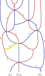
Figure 25. A Demazure weave for $\beta=11221122$ and a cycle $\gamma_{v}$ for the topmost trivalent vertex. At the bottom, we also include the sequence of roots $\rho_{k}$, where we denote $\alpha_{ij}:=\alpha_{i}+\cdots+\alpha_{j}$ for $i<j$.

The mutable part of the quiver has type $A_{2}$ and there are three frozen variables, as follows:

where the dashed arrows have weight $1/2$ and the solid arrows have weight $1$. A direct computation yields the following three frozen variables

$$z_{4},~{}z_{6},~{}\ \mathrm{and}\ F:=-z_{2}z_{5}z_{6}z_{8}+z_{2}z_{4}z_{7}z_{8}-z_{2}z_{4}+z_{2}z_{8}-z_{6}z_{8}$$

and two mutable cluster variables are

$$A_{1}:=-z_{5}z_{6}+z_{4}z_{7}+1,\ A_{2}:=-z_{5}z_{6}z_{8}+z_{4}z_{7}z_{8}-z_{4}+z_{8}.$$

For the right inductive weave the frozen variables are the same and the cluster variables are

$$z_{2},\quad A_{3}:=-z_{2}z_{5}z_{6}+z_{2}z_{4}z_{7}+z_{2}-z_{6}.$$

For the left inductive weave the frozen variables are also the same and the cluster variables are $z_{8}$ and $A_{2}$. Note that

$$A_{1}=\frac{A_{3}+z_{6}}{z_{2}},\ A_{2}=\frac{FA_{1}+z_{4}z_{6}}{A_{3}},\ z_{8}=\frac{A_{2}+z_{4}}{A_{1}},\ z_{2}=\frac{F+z_{6}z_{8}}{A_{2}},\ z_{8}=\frac{F+z_{2}z_{4}}{A_{3}}.$$

In particular, we have a cycle of mutations

$$(A_{1},A_{2})-(A_{1},A_{3})-(z_{2},A_{3})-(z_{2},z_{8})-(z_{8},A_{2})-(A_{1},A_{2}).$$

11.2. Braid relation as a mutation

Consider the braid word $\beta=112211121$ (compare with Figure 7). The cluster variables for the right inductive weave $\overrightarrow{\mathfrak{w}}(\beta)$ are

$$A_{1}=z_{2},\ A_{2}=z_{4},\ A_{3}=z_{6},\ A_{4}=z_{6}z_{7}-1,$$

$$A_{5}=-z_{2}z_{5}z_{6}z_{7}+z_{2}z_{4}z_{8}+z_{2}z_{5}+z_{2}z_{7}-z_{6}z_{7}+1,\ A_{6}=z_{4}z_{6}z_{7}z_{9}-z_{4}z_{6}z_{8}-z_{4}z_{9}-1,$$

and the quiver $Q_{\overrightarrow{\mathfrak{w}}(\beta)}$ is

Next, consider the six-valent vertex $112211\underline{121}\to 112211212$ followed by the right inductive weave (compare with Figure 8). The cluster variables are the same as above except for

$$\widetilde{A_{4}}:=-z_{2}z_{5}z_{6}+z_{2}z_{4}z_{9}+z_{2}-z_{6},$$

and the new quiver reads

The quivers are related by a mutation at $A_{4}$ and indeed we also have the mutation identity

$$\widetilde{A_{4}}=\frac{A_{3}A_{5}+A_{1}A_{6}}{A_{4}}.$$

11.3. An example with an affine type cluster algebra

Consider the braid word $\beta=213223122132$. The corresponding right inductive weave $\mathfrak{W}$ and the quiver are shown in Figure 26. The corresponding (Legendrian) link is $\Lambda(\beta_{11})$ in [16, Section 1.2], where it is also referred to as $\Lambda(\tilde{A}_{2,1})$.

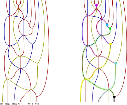
Figure 26. The inductive weave for $\beta=\sigma_{2}\sigma_{1}\sigma_{3}\sigma_{2}\sigma_{2}\sigma_{3}\sigma_{1}\sigma_{2}\sigma_{2}\sigma_{1}\sigma_{3}\sigma_{2}$ on the left, and the weave with its distinguished cycles on the right. Each cycle only takes weights $0$ or $1$, and we color the edges were the cycle takes weight $1$.

A direct computation yields the following cluster variables, ordered from top to bottom:

$$A_{1}=z_{5},A_{2}=-z_{6}z_{7}+z_{5}z_{8},A_{3}=-z_{6}z_{7}z_{9}+z_{5}z_{8}z_{9}-z_{5},A_{4}=-z_{6}z_{9}+z_{5}z_{10},$$

$$A_{5}=-z_{7}z_{9}+z_{5}z_{11},A_{6}=z_{6}z_{7}z_{10}z_{11}-z_{5}z_{8}z_{10}z_{11}-z_{6}z_{7}z_{9}z_{12}+z_{5}z_{8}z_{9}z_{12}-z_{8}z_{9}+z_{7}z_{10}+z_{6}z_{11}-z_{5}z_{12}+1.$$

The variables $A_{1},A_{2},A_{3}$ are mutable and $A_{4},A_{5},A_{6}$ are frozen. The quiver $Q_{\mathfrak{W}}$ read from $\mathfrak{W}$ is

The mutable part of $Q_{\mathfrak{W}}$ is a quiver of affine type $A$. One can verify directly that mutating at all mutable vertices creates regular functions:

$$\frac{A_{1}+A_{3}}{A_{2}}=z_{9},\qquad\frac{A_{2}A_{4}A_{5}+A_{1}^{2}A_{6}}{A_{3}}=z_{6}z_{7}z_{9}-z_{5}z_{7}z_{10}-z_{5}z_{6}z_{11}+z_{5}^{2}z_{12}-z_{5},$$

$$\begin{array}[]{rl}\displaystyle{\frac{A_{2}A_{4}A_{5}+A_{3}^{2}}{A_{1}}}=&-z_{6}z_{7}z_{8}z_{9}^{2}+z_{5}z_{8}^{2}z_{9}^{2}+z_{6}z_{7}^{2}z_{9}z_{10}-z_{5}z_{7}z_{8}z_{9}z_{10}+z_{6}^{2}z_{7}z_{9}z_{11}+\\ &-z_{5}z_{6}z_{8}z_{9}z_{11}-z_{5}z_{6}z_{7}z_{10}z_{11}+z_{5}^{2}z_{8}z_{10}z_{11}+2z_{6}z_{7}z_{9}-2z_{5}z_{8}z_{9}+z_{5}\end{array}$$

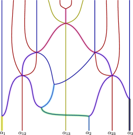
Figure 27. The weave $\mathfrak{W}^{\prime}$ for $\sigma_{1}\sigma_{2}\sigma_{2}\sigma_{1}\sigma_{3}\sigma_{2}\sigma_{2}\sigma_{3}\sigma_{1}\sigma_{2}\sigma_{2}\sigma_{1}$.

Finally, let us now apply the cyclic rotation $\sigma_{2}\sigma_{1}\sigma_{3}\sigma_{2}\sigma_{2}\sigma_{3}\sigma_{1}\sigma_{2}\sigma_{2}\sigma_{1}\sigma_{3}\sigma_{2}\mapsto\sigma_{1}\sigma_{2}\sigma_{2}\sigma_{1}\sigma_{3}\sigma_{2}\sigma_{2}\sigma_{3}\sigma_{1}\sigma_{2}\sigma_{2}\sigma_{1}$. A weave $\mathfrak{W}^{\prime}$ for the latter word is given in Figure 27.

The cluster variables for $\mathfrak{W}^{\prime}$ are the following regular functions, note that they are polynomials in $(z_{i})$:

$$B_{1}=z_{7},\ B_{2}=-z_{8}z_{9}+z_{7}z_{10},\ B_{3}=-z_{4}z_{7}+z_{3}z_{8},\ B_{4}=-z_{3}z_{8}z_{9}+z_{3}z_{7}z_{10}-z_{7},$$

$$B_{5}=-z_{3}z_{8}z_{9}z_{11}+z_{3}z_{7}z_{10}z_{11}-z_{3}z_{7}-z_{7}z_{11},\ B_{6}=-z_{8}z_{11}+z_{7}z_{12}.$$

Here $B_{3},B_{5},B_{6}$ are frozen and $B_{1},B_{2},B_{4}$ are mutable. The quiver has the form:

The cyclic rotation $z_{i}\to z_{i-2}$ sends $B_{1}$ to $A_{1}$, $B_{2}$ to $A_{2}$ and $B_{6}$ to $A_{4}$ .

11.4. An example in non-simply laced type

Consider the word $\beta=\sigma_{1}\sigma_{1}\sigma_{2}\sigma_{2}\sigma_{1}\sigma_{2}\sigma_{2}\sigma_{1}\sigma_{2}\in W(B_{2})$, the Weyl group of type $B_{2}$. In Figure 28 we draw its right inductive weave, as well as the unfolding of this weave to $A_{3}$. Note that the quiver for the $A_{3}$ weave is given by:

This quiver has a $\mathbb{Z}_{2}$-symmetry $1\leftrightarrow 1^{\prime}$, $4\leftrightarrow 4^{\prime}$, and the exchange matrix for the $B_{2}$-weave is obtained from the quiver via folding.

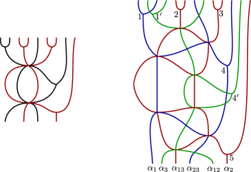
Figure 28. The right inductive weave for $\sigma_{1}\sigma_{1}\sigma_{2}\sigma_{2}\sigma_{1}\sigma_{2}\sigma_{2}\sigma_{1}\sigma_{2}\in W(B_{2})$, and its unfolding to $A_{3}$.

The symmetry acts on $z$-variables by swapping $z_{1}\leftrightarrow z_{2}$, $z_{3}\leftrightarrow z_{4}$, $z_{7}\leftrightarrow z_{8}$, $z_{11}\leftrightarrow z_{12}$ and fixing $z_{5},z_{6},z_{9},z_{10},z_{13}$, so we have an inclusion of braid varieties

$$X_{B_{2}}(\beta)\subset X_{A_{3}}(\sigma_{1}\sigma_{3}\sigma_{1}\sigma_{3}\sigma_{2}\sigma_{2}\sigma_{1}\sigma_{3}\sigma_{2}\sigma_{2}\sigma_{1}\sigma_{3}\sigma_{2})$$

where the left hand side is cut out by the equations

$$z_{1}=z_{2},\ z_{3}=z_{4},\ z_{7}=z_{8},\ z_{11}=z_{12}.$$

The $A_{3}$ cluster variables are

$$A^{\prime}_{1}=z_{3},\ A^{\prime}_{1^{\prime}}=z_{4},\ A^{\prime}_{2}=z_{6},A^{\prime}_{3}=z_{10},$$

$$A^{\prime}_{4}=-z_{4}z_{8}z_{10}+z_{4}z_{6}z_{11}-z_{10},A^{\prime}_{4^{\prime}}=-z_{3}z_{7}z_{10}+z_{3}z_{6}z_{12}-z_{10},A^{\prime}_{5}=-z_{6}z_{11}z_{12}+z_{6}z_{10}z_{13}-z_{10}.$$

Restricting these to the $B_{2}$ braid variety yields

$$A^{\prime}_{1}|_{X_{B_{2}}(\beta)}=A^{\prime}_{1^{\prime}}|_{X_{B_{2}}(\beta)},\ A^{\prime}_{4}|_{X_{B_{2}}(\beta)}=A^{\prime}_{4^{\prime}}|_{X_{B_{2}}(\beta)},$$

as expected. The cluster variables for the $B_{2}$-braid variety are $A_{1}=A^{\prime}_{1}|_{X_{B_{2}}(\beta)}=A^{\prime}_{1^{\prime}}|_{X_{B_{2}}(\beta)}$, $A_{2}=A^{\prime}_{2}|_{X_{B_{2}}(\beta)}$, $A_{3}=A^{\prime}_{3}|_{X_{B_{2}}(\beta)}$, $A_{4}=A^{\prime}_{4}|_{X_{B_{2}}(\beta)}=A^{\prime}_{4^{\prime}}|_{X_{B_{2}}(\beta)}$ and $A_{5}=A^{\prime}_{5}|_{X_{B_{2}}(\beta)}$. The exchange matrix and antisymmetrizer for $X_{B_{2}}(\beta)$ are given by

$$\varepsilon=\left(\begin{matrix}0&0&-1&1&0\\ 0&0&-1&0&1\\ 2&1&0&-2&1\\ -1&0&1&0&1/2\\ 0&-1&-1&-1&0\end{matrix}\right),\qquad d=(2,1,1,2,1)$$

so that $\varepsilon_{ij}d^{-1}_{j}$ is skew-symmetric. Mutating at $A_{3}$, for example, we obtain:

$$\frac{A_{1}^{2}A_{2}A_{5}+A_{4}^{2}}{A_{3}}=\frac{(A^{\prime}_{1}A^{\prime}_{1^{\prime}}A^{\prime}_{2}A^{\prime}_{5}+A^{\prime}_{4}A^{\prime}_{4^{\prime}})|_{X_{B_{2}}(\beta)}}{A^{\prime}_{3}|_{X_{B_{2}}(\beta)}}$$

that is regular since it is the restriction of a regular function on the larger braid variety.

References

- [1] Georgia Benkart, Seok-Jin Kang, Se-jin Oh, and Euiyong Park. Construction of irreducible representations over Khovanov-Lauda-Rouquier algebras of finite classical type. Int. Math. Res. Not. IMRN, (5):1312–1366, 2014.
- [2] Arkady Berenstein, Sergey Fomin, and Andrei Zelevinsky. Cluster algebras. III. Upper bounds and double Bruhat cells. Duke Math. J., 126(1):1–52, 2005.
- [3] Arkady Berenstein and Andrei Zelevinsky. Tensor product multiplicities, canonical bases and totally positive varieties. Inventiones mathematicae, 143(1):77–128, 2001.
- [4] Anders Bjorner and Francesco Brenti. Combinatorics of Coxeter groups, volume 231. Springer Science & Business Media, 2006.
- [5] Philip Boalch. Stokes matrices, Poisson Lie groups and Frobenius manifolds. Invent. Math., 146(3):479–506, 2001.
- [6] Philip Boalch. Quasi-Hamiltonian geometry of meromorphic connections. Duke Math. J., 139(2):369–405, 2007.
- [7] Philip Boalch. Wild character varieties, points on the Riemann sphere and Calabi’s examples. In Representation theory, special functions and Painlevé equations—RIMS 2015, volume 76 of Adv. Stud. Pure Math., pages 67–94. Math. Soc. Japan, Tokyo, 2018.
- [8] K. A. Brown, K. R. Goodearl, and M. Yakimov. Poisson structures on affine spaces and flag varieties. I. Matrix affine Poisson space. Adv. Math., 206(2):567–629, 2006.
- [9] A. B. Buan, O. Iyama, I. Reiten, and J. Scott. Cluster structures for 2-Calabi-Yau categories and unipotent groups. Compos. Math., 145(4):1035–1079, 2009.
- [10] Eric Bucher and John Machacek. Reddening sequences for Banff quivers and the class . SIGMA Symmetry Integrability Geom. Methods Appl., 16:Paper No. 049, 11, 2020.
- [11] Peigen Cao. On exchange matrices from string diagrams. arXiv preprint arXiv:2203.07822, 2022.
- [12] Peigen Cao and Bernhard Keller. On Leclerc’s conjectural cluster structures for open Richardson varieties. arXiv preprint arXiv:2207.10184, 2022.
- [13] Roger Casals and Honghao Gao. Infinitely many Lagrangian fillings. Ann. of Math. (2), 195(1):207–249, 2022.
- [14] Roger Casals, Eugene Gorsky, Mikhail Gorsky, and José Simental. Algebraic weaves and braid varieties. arXiv preprint arXiv:2012.06931, 2020.
- [15] Roger Casals, Eugene Gorsky, Mikhail Gorsky, and José Simental. Positroid links and braid varieties. arXiv preprint arXiv:2105.13948, 2021.
- [16] Roger Casals and Lenhard Ng. Braid loops with infinite monodromy on the Legendrian contact DGA. arXiv preprint arXiv:2101.02318, 2021.
- [17] Roger Casals and Daping Weng. Microlocal theory of Legendrian links and cluster algebras. arXiv preprint arXiv:2204.13244, 2022.
- [18] Roger Casals and Eric Zaslow. Legendrian weaves: -graph calculus, flag moduli and applications. Geometry & Topology, to appear.
- [19] Cesar Ceballos, Jean-Philippe Labbé, and Christian Stump. Subword complexes, cluster complexes, and generalized multi-associahedra. J. Algebraic Combin., 39(1):17–51, 2014.
- [20] Neil Chriss and Victor Ginzburg. Representation theory and complex geometry. Modern Birkhäuser Classics. Birkhäuser Boston, Ltd., Boston, MA, 2010. Reprint of the 1997 edition.
- [21] Ben Elias. A diamond lemma for Hecke-type algebras. Transactions of the American Mathematical Society, 375(03):1883–1915, 2022.
- [22] Ben Elias and Geordie Williamson. Soergel calculus. Representation Theory of the American Mathematical Society, 20(12):295–374, 2016.
- [23] Laura Escobar. Brick manifolds and toric varieties of brick polytopes. Electron. J. Combin., 23(2):Paper 2.25, 18, 2016.
- [24] V. V. Fock and A. B. Goncharov. Cluster -varieties, amalgamation, and Poisson-Lie groups. In Algebraic geometry and number theory, volume 253 of Progr. Math., pages 27–68. Birkhäuser Boston, 2006.
- [25] Vladimir Fock and Alexander Goncharov. Moduli spaces of local systems and higher Teichmüller theory. Publ. Math. Inst. Hautes Études Sci., (103):1–211, 2006.
- [26] Vladimir V. Fock and Alexander B. Goncharov. Cluster ensembles, quantization and the dilogarithm. Ann. Sci. Éc. Norm. Supér. (4), 42(6):865–930, 2009.
- [27] Sergey Fomin, Michael Shapiro, and Dylan Thurston. Cluster algebras and triangulated surfaces. I. Cluster complexes. Acta Math., 201(1):83–146, 2008.
- [28] Sergey Fomin, Lauren Williams, and Andrei Zelevinsky. Introduction to Cluster Algebras. chapter 6. arXiv preprint arXiv:2008.09189, 2020.
- [29] Sergey Fomin and Andrei Zelevinsky. Double Bruhat cells and total positivity. J. Amer. Math. Soc., 12(2):335–380, 1999.
- [30] Sergey Fomin and Andrei Zelevinsky. Cluster algebras. I. Foundations. J. Amer. Math. Soc., 15(2):497–529, 2002.
- [31] Sergey Fomin and Andrei Zelevinsky. Cluster algebras II. Invent. Math., 154(1):63–121, 2003.
- [32] Chris Fraser. Quasi-homomorphisms of cluster algebras. Adv. in Appl. Math., 81:40–77, 2016.
- [33] Chris Fraser and Melissa Sherman-Bennett. Positroid cluster structures from relabeled plabic graphs. Alg. Comb., to appear.
- [34] Pavel Galashin and Thomas Lam. The twist for Richardson varieties. arXiv preprint arXiv:2204.05935, 2022.
- [35] Pavel Galashin and Thomas Lam. Positroid varieties and cluster algebras. Ann. Sci. Éc. Norm. Supér., to appear.
- [36] Pavel Galashin, Thomas Lam, Melissa Sherman-Bennett, and David Speyer. Braid variety cluster structures, I: 3D plabic graphs, in progress.
- [37] Pavel Galashin, Thomas Lam, Melissa Sherman-Bennett, and David Speyer. Braid variety cluster structures, II: general type, in progress.
- [38] Honghao Gao, Linhui Shen, and Daping Weng. Augmentations, fillings, and clusters. arXiv preprint arXiv:2008.10793, 2020.
- [39] Christof Geiss, Bernard Leclerc, and Jan Schröer. Partial flag varieties and preprojective algebras. Ann. Inst. Fourier (Grenoble), 58(3):825–876, 2008.
- [40] Christof Geiß, Bernard Leclerc, and Jan Schröer. Kac-Moody groups and cluster algebras. Adv. Math., 228(1):329–433, 2011.
- [41] Christof Geiss, Bernard Leclerc, and Jan Schröer. Factorial cluster algebras. Doc. Math., 18:249–274, 2013.
- [42] Michael Gekhtman, Michael Shapiro, and Alek Vainshtein. Cluster algebras and Poisson geometry. Number 167. American Mathematical Soc., 2010.
- [43] Alexander Goncharov and Linhui Shen. Donaldson–thomas transformations of moduli spaces of g-local systems. Advances in Mathematics, 327:225–348, 2018.
- [44] Alexander Goncharov and Linhui Shen. Quantum geometry of moduli spaces of local systems and representation theory. arXiv preprint arXiv:1904.10491, 2019.
- [45] Mark Gross, Paul Hacking, and Sean Keel. Birational geometry of cluster algebras. Algebr. Geom., 2(2):137–175, 2015.
- [46] Mark Gross, Paul Hacking, Sean Keel, and Maxim Kontsevich. Canonical bases for cluster algebras. J. Amer. Math. Soc., 31(2):497–608, 2018.
- [47] Paul Hacking and Sean Keel. Mirror symmetry and cluster algebras. In Proceedings of the ICM 2018. Vol. II. Invited lectures, pages 671–697. World Sci. Publ., 2018.
- [48] Grace Ingermanson. Cluster Algebras of Open Richardson Varieties. ProQuest LLC, Ann Arbor, MI, 2019. Thesis (Ph.D.)–University of Michigan.
- [49] Tamás Kálmán. Braid-positive Legendrian links. Int. Math. Res. Not., pages Art ID 14874, 29, 2006.
- [50] Joel Kamnitzer. Mirković-Vilonen cycles and polytopes. Annals of mathematics, 171(1):245–294, 2010.
- [51] Bernhard Keller. Quiver mutation and combinatorial DT-invariants. Discrete Mathematics and Theoretical Computer Science, 2017.
- [52] Bernhard Keller and Laurent Demonet. A survey on maximal green sequences. Representation theory and beyond, 758:267–286, 2020.
- [53] Sefi Ladkani. On cluster algebras from once punctured closed surfaces. arXiv preprint arXiv:1310.4454, 2013.
- [54] Thomas Lam and David E. Speyer. Cohomology of cluster varieties I: Locally acyclic case. Algebra Number Theory, 16(1):179–230, 2022.
- [55] Bernard Leclerc. Cluster structures on strata of flag varieties. Adv. Math., 300:190–228, 2016.
- [56] G. Lusztig. Total positivity in reductive groups. In Lie theory and geometry, volume 123 of Progr. Math., pages 531–568. Birkhäuser Boston, Boston, MA, 1994.
- [57] George Lusztig. Introduction to quantum groups, volume 110 of Progress in Mathematics. Birkhäuser Boston, Inc., Boston, MA, 1993.
- [58] Bethany Marsh and Konstanze Rietsch. Parametrizations of flag varieties. Representation Theory of the American Mathematical Society, 8(9):212–242, 2004.
- [59] Anton Mellit. Cell decompositions of character varieties. arXiv preprint arXiv:1905.10685, 2019.
- [60] Etienne Ménard. Cluster algebras associated with open Richardson varieties: an algorithm to compute initial seeds. arXiv preprint arXiv:2201.10292, 2022.
- [61] Matthew R Mills. On the relationship between green-to-red sequences, local-acyclicity, and upper cluster algebras. arXiv preprint arXiv:1804.00479, 2018.
- [62] Greg Muller. Locally acyclic cluster algebras. Adv. Math., 233:207–247, 2013.
- [63] Greg Muller. The existence of a maximal green sequence is not invariant under quiver mutation. The Electronic Journal of Combinatorics, 23(2):P2–47, 2016.
- [64] Greg Muller. Skein and cluster algebras of marked surfaces. Quantum Topology, 7(3):435–503, 2016.
- [65] Fan Qin. Bases for upper cluster algebras and tropical points. To appear in J. Eur. Math. Soc.
- [66] Jeanne Scott. Grassmannians and cluster algebras. Proc. London Math. Soc. (3), 92(2):345–380, 2006.
- [67] K. Serhiyenko, M. Sherman-Bennett, and L. Williams. Cluster structures in Schubert varieties in the Grassmannian. Proc. Lond. Math. Soc. (3), 119(6):1694–1744, 2019.
- [68] Linhui Shen and Daping Weng. Cluster structures on double Bott-Samelson cells. Forum Math. Sigma, 9:Paper No. e66, 89, 2021.
- [69] Yasutaka Sibuya. Global theory of a second order linear ordinary differential equation with a polynomial coefficient. North-Holland Publishing Co., Amsterdam-Oxford; American Elsevier Publishing Co., Inc., New York, 1975. North-Holland Mathematics Studies, Vol. 18.
- [70] Ben Webster and Milen Yakimov. A Deodhar-type stratification on the double flag variety. Transform. Groups, 12(4):769–785, 2007.
- [71] Daping Weng. Donaldson-Thomas transformation of double Bruhat cells in semisimple Lie groups. Ann. Sci. Éc. Norm. Supér. (4), 53(2):353–436, 2020.