Temperature-dependent dielectric function of intrinsic silicon:
Analytic models and atom-surface potentials

Abstract

The optical properties of monocrystalline, intrinsic silicon are of interest for technological applications as well as fundamental studies of atom-surface interactions. For an enhanced understanding, it is of great interest to explore analytic models which are able to fit the experimentally determined dielectric function $\epsilon(T_{\Delta},\omega)$, over a wide range of frequencies and a wide range of the temperature parameter $T_{\Delta}=(T-T_{0})/T_{0}$, where $T_{0}=293\,{\rm K}$ represents room temperature. Here, we find that a convenient functional form for the fitting of the dielectric function of silicon involves a Lorentz-Dirac curve with a complex, frequency-dependent amplitude parameter, which describes radiation reaction. We apply this functional form to the expression $[\epsilon(T_{\Delta},\omega)-1]/[\epsilon(T_{\Delta},\omega)+2]$, inspired by the Clausius-Mossotti relation. With a very limited set of fitting parameters, we are able to represent, to excellent accuracy, experimental data in the (angular) frequency range $0<\omega<0.16\,{\rm a.u.}$ and $0<T_{\Delta}<2.83$, corresponding to the temperature range $293\,{\rm K}<T<1123\,{\rm K}$. Using our approach, we evaluate the short-range $C_{3}$ and the long-range $C_{4}$ coefficients for the interaction of helium atoms with the silicon surface. In order to validate our results, we compare to a separate temperature-dependent direct fit of $\epsilon(T_{\Delta},\omega)$ to the Lorentz-Dirac model.

I Introduction

Because of its enormous technological importance, the optical properties of monocrystalline, undoped silicon, sometimes referred to as intrinsic silicon, have been investigated in great detail over the past decades [1, 2, 3, 4, 5, 6, 7, 8, 9, 10, 11, 12, 13, 14, 15, 16, 17, 18, 19, 20, 21, 22, 23, 24, 25]. The determination of an appropriate analytic model for the frequency-dependent, and temperature-dependent, dielectric function also is of prime interest, especially because it may give insight into the physical mechanism that generates the response of the medium [21, 22]. In general, it is of obvious interest to find a satisfactory representation of the available data for the dielectric function of silicon, using the most simple analytic functional form possible. The aims of our paper are as follows: (i) We explore the applicability of simple functional forms, which we refer to as the Clausius-Mossotti and Lorentz-Dirac models (which include radiation reaction damping terms) for the frequency- and temperature-dependent dielectric function of silicon. (ii) We aim to describe the temperature dependence of the dielectric function of intrinsic silicon, using an efficient model, i.e., using a small number of fitting parameters. Finally, (iii) we aim to demonstrate the applicability of the functional forms of the temperature- and frequency-dependent dielectric function for the calculation of a practically important quantity, namely, the short-range ($C_{3}$) and long-range ($C_{4}$) coefficients of the atom-surface interaction for a few simple atomic systems interacting with intrinsic silicon.

We have carefully examined available data sets for the real and imaginary parts of the dielectric function of silicon and base our investigations on Refs. [13, 20, 23, 14, 19] (see also a pertinent comprehensive discussion in Appendix A.1). For these data sets, which cover the temperature range $293\,{\rm K}<T<1123\,{\rm K}$, we attempt to find a uniform, simple, temperature-dependent analytic model for the dielectric function of monocrystalline (intrinsic) silicon. Our motivation is twofold. First, such an analytic model could be of interest for practical applications, and second, the most appropriate functional form for the description of the dielectric function might otherwise give insight into the physical mechanism underlying the optical response of the medium. In Ref. [21], it is pointed out that a two-resonance analytic model of the Lorentz-Dirac (LD) type can successfully describe the experimental data for the Si dielectric function over wide frequency ranges. A physical interpretation and justification for the functional form used in Ref. [21] is given in Refs. [22, 25]. This justification [21, 22, 25] is based on the so-called Lorentz–Dirac force (see Sec. 8.6.2 of Ref. [26] and Appendix A.2). A second fitting method, which we also apply here, tries to augment the Lorentz-Dirac approach using a functional form inspired by the Clausius-Mossotti (CM) relation. The aim of the latter approach is to take into account the local-field effect inside the crystal. The dual fitting method has been used in Ref. [27] where it has been shown that the Lorentz-Dirac and Clausius-Mossotti functional forms (without the radiation reaction term) can be mapped onto each other on the basis of a simple resonance frequency shift detailed in Eq. (12) of Ref. [27]. (We note that the Clausius-Mossotti functional form is referred to as the Lorentz-Lorenz formula in Ref. [27].) Here, we aim to explore if similar conclusions can be drawn when the model is augmented by a radiation reaction term in the numerator of the resonance functional forms, and in an application to the dielectric function of a real material rather than a model problem. A further motivation for our study comes from the fact that a number of density-functional theory (DFT) and Bethe-Salpeter based approaches [28, 29, 30, 31, 32, 33], TDDFT [29, 30, 31, 33], as well as QED-TDDFT frameworks [34, 35, 36, 37] suggest that the excitonic mechanism governing the dielectric function of silicon supports a functional form of the type explored here.

In order to ramify the motivation for our investigations, let us mention two additional aspects originating in fundamental physics. The first is the potential use of silicon in gravitational wave detection experiments, where an accurate understanding of the optical properties is crucial to gauge the achievable interferometric contrast [24]. The second is the use of monocrystalline silicon as a substrate for atom-surface studies, notably, at the Heidelberg Spin-Echo Atomic Beam Apparatus (see Refs. [38, 39, 40]). We here evaluate the temperature dependence of the Casimir coefficients $C_{3}$ (short-range) and $C_{4}$ (long-range), which represent the asymptotics of the atom-surface interaction energy, for helium (and other) atoms interacting with monocrystalline silicon. Helium has been of prime experimental interest and takes a very special role in atom-surface studies [41, 42, 43, 44], and we devote special attention to the helium system here. Details of other atoms are relegated to Ref. [45]. We can anticipate that our two fitting methods lead to consistent numerical results for the short-range $C_{3}$, and long-range $C_{4}$ coefficients.

The paper is organized as follows. In Sec. II, we discuss the fitting of the dielectric function of intrinsic silicon to convenient functional forms. Specifically, in Sec. II.1, a functional form (a “master function”) is indicated which will be used for our fitting in the following. (The physical justification of the “master function” is discussed on the basis of the Lorentz-Dirac equation.) In Sec. II.2, we discuss an approach to the fitting of the temperature-dependent dielectric function of silicon, which we refer to as the Clausius-Mossotti approach. This approach is based on the comparison of a specific ratio involving the dielectric function, to a generalized Lorentz-Dirac functional form, with complex oscillator strengths. The latter functional form constitutes our “master function”. In Sec. II.3, we discuss, for comparison, an alternative approach to the description of the temperature-dependent dielectric function based on the Lorentz-Dirac approach. In Sec. III, we perform the evaluation of the coefficients $C_{3}$ and $C_{4}$ for helium interacting with silicon. Conclusions are presented in Sec. IV. SI mksA units are used throughout the paper.

Table 1: Coefficients resulting from Clausius-Mossotti fitting, as described in Eqs. (9) and (10), are given for the first resonance of monocrystalline silicon over a range of temperatures $0<T_{\Delta}<2.83$. Here, $E_{h}$ is the Hartree energy and $\hbar$ is Planck’s constant.

$T_{\Delta}$	$a_{1}^{\mathrm{CM}}$	$\omega_{1}^{\mathrm{CM}}\,[E_{h}/\hbar]$	$\gamma_{1}^{\mathrm{CM}}\,[E_{h}/\hbar]$	$\gamma^{\prime\mathrm{CM}}_{1}\,[E_{h}/\hbar]$
0.000	0.004943	0.1293	0.01841	0.1306
0.273	0.004856	0.1277	0.01973	0.1392
0.444	0.004564	0.1266	0.01964	0.1474
0.614	0.004715	0.1264	0.02030	0.1403
0.785	0.004508	0.1258	0.02059	0.1440
0.956	0.004647	0.1256	0.02075	0.1355
1.126	0.004586	0.1249	0.02139	0.1405
1.397	0.004903	0.1247	0.02221	0.1284
1.468	0.005163	0.1243	0.02287	0.1173
1.638	0.005588	0.1237	0.02529	0.1179
2.321	0.007875	0.1242	0.03141	0.0614
2.833	0.008155	0.1231	0.03376	0.0608

II Dielectric Function of Silicon

II.1 Lorentz-Dirac and Master Function

In Refs. [21, 22, 25], the authors advocate to fit experimental data for the dielectric function of a reference material via a functional form of the Lorentz-–Dirac type, which is essentially equal to the Sellmeier form [46], but with a complex amplitude parameter (which could be understood as a complex oscillator strength), which takes the radiation reaction into account. Details of the derivation of the functional form have been discussed at length in the literature, and they are recalled for the convenience of the reader in Appendix A.2 where we lay special emphasis on the sign of the imaginary part of the numerator term. As a result of these considerations, we are motivated to define the functional form $f(T_{\Delta},\omega)$, which we refer to as the Lorentz–Dirac master function, as follows:

$$f(T_{\Delta},\omega)=\sum_{k=1}^{k_{\rm max}}\frac{a_{k}(\omega_{k}^{2}-\mathrm{i}\gamma_{k}^{\prime}\omega)}{\omega_{k}^{2}-\omega^{2}-i\omega\gamma_{k}}\,,$$ (1)

with the dimensionless temperature parameter

$$T_{\Delta}=\frac{T-T_{0}}{T_{0}}\,,$$ (2)

where $T_{0}=293$ K. In Eq. (1), the resonance energies $\omega_{k}$, the radiation reaction damping constants $\gamma_{k}^{\prime}$ and level widths $\gamma_{k}$, and the amplitudes $a_{k}$ all depend on $T_{\Delta}$. The functional form given in Eq. (1) has a propagator denominator equal to that of a damped harmonic oscillator while the numerator (the oscillator strength) has a nonvanishing imaginary part. The parameter $k_{\rm max}$ terminates the sum over the generalized damped oscillator terms; as we will show, the sum over oscillators leads to a satisfactory representation of the dielectric function with only few terms, resulting in $k_{\rm max}$ being a small integer.

Table 2: We present the analog of Table 1 for the second resonance of monocrystalline silicon.

$T_{\Delta}$	$a_{2}^{\mathrm{CM}}$	$\omega_{2}^{\mathrm{CM}}\,[E_{h}/\hbar]$	$\gamma_{2}^{\mathrm{CM}}\,[E_{h}/\hbar]$	$\gamma^{\prime\mathrm{CM}}_{2}\,[E_{h}/\hbar]$
0.000	0.7709	0.3117	0.0990	0.0971
0.273	0.7739	0.3135	0.1066	0.1057
0.444	0.7761	0.3135	0.1173	0.1176
0.614	0.7766	0.3133	0.1191	0.1193
0.785	0.7780	0.3138	0.1242	0.1247
0.956	0.7783	0.3129	0.1293	0.1307
1.126	0.7796	0.3136	0.1336	0.1351
1.397	0.7804	0.3130	0.1363	0.1381
1.468	0.7815	0.3122	0.1424	0.1447
1.638	0.7847	0.3128	0.1333	0.1295
2.321	0.7869	0.3072	0.1194	0.1121
2.833	0.7949	0.3117	0.1159	0.1016

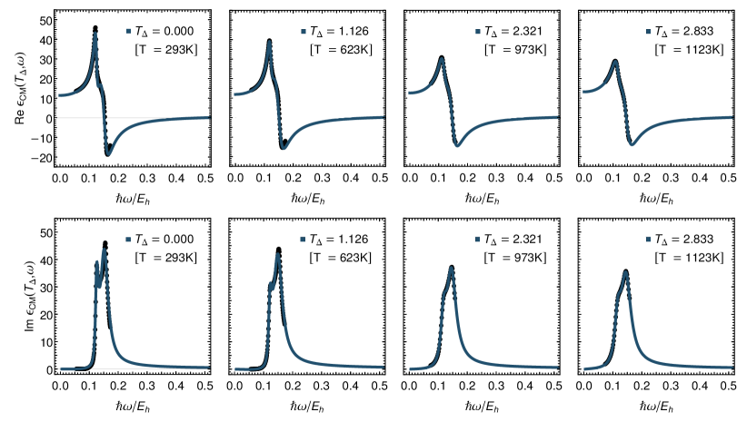
Figure 1: Real (top row) and Imaginary (bottom row) parts of the dielectric function $\epsilon_{\mathrm{CM}}(T_{\Delta},\omega)$ are plotted as functions of the angular frequency $\omega$, for monocrystalline (undoped, intrinsic) silicon for various temperatures. Experimental data [23, 13] (dotted) is shown to be in agreement with the CM fit (blue) defined in Eq. (4) for temperature-dependent parameters given in Eq. (11) and coefficients in Table 3. Note that the quantity $\hbar\omega/E_{h}$ is equal to the angular frequency expressed in atomic units. Eight additional temperatures, between $T_{\Delta}=0$ and $T_{\Delta}=2.83$, namely, the values $T_{\Delta}=0.273$, $0.444$, $0.614$, $0.785$, $0.956$, $1.297$, $1.468$, and $1.638$, are considered in Ref. [45].

Before we discuss the actual fitting procedure, it is instructive to ask how the specific form of $f(T_{\Delta},\omega)$ can be justified from first-principles theory. The ab initio calculation of the dielectric function of a material is a two-step process: first, the electronic band structure is obtained, either using density-functional theory (DFT) or Green’s function based approaches [28, 32]. In the second step, the band structure is taken as input to obtain the optical excitation spectrum of the material via linear-response theory. To reproduce the double-peak structure of the optical absorption spectrum of Si, it is essential to capture excitonic effects. This can be accomplished using the Bethe-Salpeter equation [28, 32] or time-dependent density-functional theory (TDDFT) [29, 30, 31, 33]. In both approaches, one first constructs a noninteracting response function and then builds in dynamical many-body effects, most notably the screened electron-hole interactions. The noninteracting response function features energy denominators of exactly the same form as in Eq. (1). It is customary to choose empirical line broadening parameters (corresponding to our $\gamma_{k}$) on the order of 0.1 - 0.2 eV to obtain optical spectra in good agreement with experiment. This simulates the lifetime broadening caused by phonons, disorder, or finite quasiparticle lifetimes [47].

Table 3: We present coefficients associated with the Clausius-Mossotti model given in Eq. (11), found from fitting the coefficients in Table 1 and Table 2 as functions of temperature, for monocrystalline silicon.

$k$	$a^{\mathrm{CM}}_{k,0}$	$a^{\mathrm{CM}}_{k,1}$	$a^{\mathrm{CM}}_{k,2}$
1	$4.870\text{\times}{10}^{-3}$	$-8.936\text{\times}{10}^{-4}$	$7.854\text{\times}{10}^{-4}$
2	$7.722\text{\times}{10}^{-1}$	$5.984\text{\times}{10}^{-3}$	$5.586\text{\times}{10}^{-4}$
$k$	$\omega^{\mathrm{CM}}_{k,0}\,[E_{h}/\hbar]$	$\omega^{\mathrm{CM}}_{k,1}\,[E_{h}/\hbar]$	$\omega^{\mathrm{CM}}_{k,2}\,[E_{h}/\hbar]$
1	$1.289\text{\times}{10}^{-1}$	$-4.571\text{\times}{10}^{-3}$	$9.421\text{\times}{10}^{-4}$
2	$3.129\text{\times}{10}^{-1}$	$6.405\text{\times}{10}^{-4}$	$-6.527\text{\times}{10}^{-4}$
$k$	$\gamma^{\mathrm{CM}}_{k,0}\,[E_{h}/\hbar]$	$\gamma^{\mathrm{CM}}_{k,1}\,[E_{h}/\hbar]$	$\gamma^{\mathrm{CM}}_{k,2}\,[E_{h}/\hbar]$
1	$1.875\text{\times}{10}^{-2}$	$9.274\text{\times}{10}^{-4}$	$1.651\text{\times}{10}^{-3}$
2	$9.742\text{\times}{10}^{-2}$	$4.814\text{\times}{10}^{-2}$	$-1.518\text{\times}{10}^{-2}$
$k$	$\gamma^{\prime\mathrm{CM}}_{k,0}\,[E_{h}/\hbar]$	$\gamma^{\prime\mathrm{CM}}_{k,1}\,[E_{h}/\hbar]$	$\gamma^{\prime\mathrm{CM}}_{k,2}\,[E_{h}/\hbar]$
1	$1.387\text{\times}{10}^{-1}$	$1.161\text{\times}{10}^{-2}$	$-1.543\text{\times}{10}^{-2}$
2	$9.505\text{\times}{10}^{-2}$	$5.607\text{\times}{10}^{-2}$	$-1.948\text{\times}{10}^{-2}$

Standard Bethe-Salpeter or TDDFT calculations of the optical absorption spectra of solids do not include any radiative reaction forces, and the resulting oscillator strengths are purely real [30]. To formally justify the parameter $\gamma_{k}^{\prime}$ in Eq. (1) one needs an ab initio approach in which the dynamics of the electrons and the photon field are coupled and treated on an equal footing, either at the classical level using Maxwell’s equations, or using QED. For the latter case, a coupled QED-TDDFT framework has been developed in the past few years [34, 35, 36, 37]. More relevant for the context of our work, Schäfer and Johansson [48] recently proposed a TDDFT formalism that includes dissipation due to classical Abraham-Lorentz-type radiative reaction forces, and presented applications to plasmonic systems. The functional forms employed here are consistent with the mechanisms underlying the DFT, TDDFT, Bethe-Salpeter and QED-TDDFT frameworks employed in the investigations which lead toward an ab initio understanding of the dielectric function. While at present, to our knowledge, there exist no first-principles calculations of the optical spectra of periodic solids including classical radiative reaction forces or QED; given the progress in the field, such results may emerge in the near future.

In Refs. [27] and [49], inspired by the Clausius–Mossotti relation, the dielectric ratio

$$\rho(T_{\Delta},\omega)=\frac{\epsilon(T_{\Delta},\omega)-1}{\epsilon(T_{\Delta},\omega)+2}\doteq f(T_{\Delta},\omega)$$ (3)

was fitted to the Lorentz–Dirac functional form, for $\alpha$-quartz. [The fitting to the functional form is indicated by the $\doteq$ sign.] In this paper, we propose to combine the advantages of the approaches outlined in Refs. [27, 21, 22, 25], namely, the inclusion of radiation reaction, and the advantage of the approach chosen in Refs. [27] and [49], which is the dense-material effect encoded in the Clausius–Mossotti relation. To this end, we first take experimental data for the temperature-dependent dielectric function of silicon, on the basis of which we calculate the dielectric ratio $\rho(T_{\Delta},\omega)$, which we then fit with $f(T_{\Delta},\omega)$. The resulting expression for the dielectric function is

$$\epsilon_{\rm CM}(T_{\Delta},\omega)\doteq\frac{1+2f(T_{\Delta},\omega)}{1-f(T_{\Delta},\omega)}\,.$$ (4)

This will be referred to as the Clausius-Mossotti (CM) fit. The more direct fit

$$\epsilon_{\rm LD}(T_{\Delta},\omega)-1\doteq f(T_{\Delta},\omega)$$ (5)

will be referred to as the Lorentz-Dirac (LD) fit. The quantity

$$\delta\epsilon(T_{\Delta},\omega)=\left|\epsilon_{\mathrm{CM}}(T_{\Delta},\omega)-\epsilon_{\mathrm{LD}}(T_{\Delta},\omega)\right|$$ (6)

measures the dependence of the fitted dielectric function on the fitting procedure. Of course, the quantity $\delta\epsilon(T_{\Delta},\omega)$ does not include experimental uncertainty pertaining to the input data [13, 20, 23, 14, 19]. For the statistical uncertainties of the fitting parameters of our model, we refer to Tables I and II of the Ref. [45].

A brief discussion is in order. While one could argue that the CM fit is favored by physical considerations [49], one should note the lack of experimental uncertainty estimates in the input data provided in Refs. [14, 19, 20]. As a byproduct of the alternative fits $\rho(T_{\Delta},\omega)\approx f(T_{\Delta},\omega)$ and $\epsilon(T_{\Delta},\omega)-1\approx f(T_{\Delta},\omega)$, we are able to estimate the uncertainty on the basis of Eq. (6). Two remarks are in order. (i) Both $\epsilon_{\mathrm{CM}}(T_{\Delta},\omega)$ as well as $\epsilon_{\mathrm{LD}}(T_{\Delta},\omega)$ fulfill the Kramers-Kronig relationships For $\epsilon_{\mathrm{LD}}(T_{\Delta},\omega)$, this has been shown explicitly in Ref. [22], while for $\epsilon_{\mathrm{CM}}(T_{\Delta},\omega)$, this follows from the relations ${\rm{Re}}[\epsilon_{\mathrm{CM}}(T_{\Delta},\omega)]={\rm{Re}}[\epsilon_{\mathrm{CM}}(T_{\Delta},-\omega)]$ and ${\rm{Im}}[\epsilon_{\mathrm{CM}}(T_{\Delta},\omega)]=-{\rm{Im}}[\epsilon_{\mathrm{CM}}(T_{\Delta},-\omega)]$. These relations allow us to invoke the formalism outlined in Sec. 6.6 of Ref. [26]. (ii) In the asymptotic limit of large $\omega$, in view of the limiting process

$$\rho(T_{\Delta},\omega)=\frac{\epsilon(T_{\Delta},\omega)-1}{\epsilon(T_{\Delta},\omega)+2}\;\;\mathop{\longrightarrow}^{\omega\to\infty}\;\;\frac{\epsilon(T_{\Delta},\omega)-1}{3}\,,$$ (7)

for $\omega\to\infty$, one has $\epsilon(T_{\Delta},\omega)\longrightarrow 1+3\rho(T_{\Delta},\omega)$. So, in the asymptotic limits, the two fitted functional forms $f(T_{\Delta},\omega)$ become equivalent up to the addition of unity, and a multiplicative factor three.

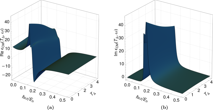
Figure 2: Real (a) and imaginary (b) parts of the Clausius-Mossotti dielectric function $\epsilon_{\mathrm{CM}}(T_{\Delta},\omega)$ as described by Eq. (4) are plotted as functions of the reduced temperature $T_{\Delta}$ and driving frequency $\omega$, for monocrystalline silicon with parameters given in Eq. (11) and coefficients in Table 3. This plot shows agreement between the CM fit shown here and the LD fit shown in Fig. 4.

II.2 Clausius-Mossotti Model

In the context of the current investigation, our aim is to find a simple and consistent fit to the dielectric function of monocrystalline (intrinsic) silicon. In the current section, we attempt to fit the dielectric ratio $\rho(T_{\Delta},\omega)$ defined in Eq. (3) to the master function given in Eq. (1). Let us first recall a few essential formulas. We denote the real and imaginary parts of the complex index of refraction by $n(\omega)$ and $k(\omega)$, respectively. These quantities are related to each other by the Kramers-Kronig relations (see, e.g., Chap. 6 of Ref. [26]). The same is true for the real and imaginary parts of the dielectric function $\epsilon(\omega)$, which is given as $\epsilon(\omega)=[n(\omega)+\mathrm{i}\,k(\omega)]^{2}$. We introduce a phenomenological description of the dielectric function by simply assuming a temperature dependence of the individual parameters in Eq. (15). This approach has been taken in Refs. [50, 19, 51]. We thus write the temperature-dependent dielectric functions as in Eq. (3),

$$\rho(T_{\Delta},\omega)=\frac{\epsilon(T_{\Delta},\omega)-1}{\epsilon(T_{\Delta},\omega)+2}\\ \approx\rho_{\mathrm{CM}}(T_{\Delta},\omega)=\frac{\epsilon_{\mathrm{CM}}(T_{\Delta},\omega)-1}{\epsilon_{\mathrm{CM}}(T_{\Delta},\omega)+2}\\ =\sum_{k=1}^{k_{\rm max}}\frac{a^{\mathrm{CM}}_{k}(T_{\Delta})\,[\,\omega^{\mathrm{CM}}_{k}(T_{\Delta})\,]^{2}-\mathrm{i}\,\gamma^{\prime\mathrm{CM}}_{k}(T_{\Delta})\,\omega)}{[\,\omega^{\mathrm{CM}}_{k}(T_{\Delta})\,]^{2}-\omega^{2}-\mathrm{i}\,\omega\,\gamma^{\mathrm{CM}}_{k}(T_{\Delta})}\,,$$ (8)

where $k$ counts the number of resonances and we have indicated the place where we employ the fitting procedure by the “$\approx$” sign.

The temperature-dependent real and imaginary parts of $\rho_{\mathrm{CM}}(T_{\Delta},\omega)$ can thus be written as follows,

$$\mathrm{Re}[\rho_{\mathrm{CM}}(T_{\Delta},\omega)]=\sum_{k=1}^{k_{\rm max}}a^{\mathrm{CM}}_{k}(T_{\Delta})\\ \times\frac{\omega^{2}\left[\,\gamma^{\mathrm{CM}}_{k}(T_{\Delta})\,\gamma_{k}^{\prime\mathrm{CM}}(T_{\Delta})-[\omega^{\mathrm{CM}}_{k}(T_{\Delta})]^{2}\,\right]+\omega^{4}}{(\omega^{2}-[\omega^{\mathrm{CM}}_{k}(T_{\Delta})]^{2})^{2}+\omega^{2}\,\left[\gamma^{\mathrm{CM}}_{k}(T_{\Delta})\right]^{2}}\,,$$ (9)

while the imaginary part is

$$\mathrm{Im}[\rho_{\mathrm{CM}}(T_{\Delta},\omega)]=\sum_{k=1}^{k_{\rm max}}a^{\mathrm{CM}}_{k}(T_{\Delta})\,\omega\,\\ \times\frac{\omega^{2}\gamma_{k}^{\prime\mathrm{CM}}(T_{\Delta})+\left\{\gamma^{\mathrm{CM}}_{k}(T_{\Delta})-\gamma_{k}^{\prime\mathrm{CM}}(T_{\Delta})\right\}[\omega^{\mathrm{CM}}_{k}(T_{\Delta})]^{2}}{\{\omega^{2}-[\omega^{\mathrm{CM}}_{k}(T_{\Delta})]^{2}\}^{2}+\omega^{2}\,\left[\,\gamma^{\mathrm{CM}}_{k}(T_{\Delta})\,\right]^{2}}.$$ (10)

Following Refs. [5, 4], the coefficients $a_{k}(T_{\Delta})$, $\omega_{k}(T_{\Delta})$, and $\gamma_{k}(T_{\Delta})$ are approximated by quadratic functions in the temperature,

$$a_{k}(T_{\Delta})= \;a^{\mathrm{CM}}_{k,0}+a^{\mathrm{CM}}_{k,1}\;T_{\Delta}+a^{\mathrm{CM}}_{k,2}\;(T_{\Delta})^{2}\,,$$ (11a)

$$\omega_{k}(T_{\Delta})= \;\omega^{\mathrm{CM}}_{k,0}+\omega^{\mathrm{CM}}_{k,1}\;T_{\Delta}+\omega^{\mathrm{CM}}_{k,2}\;(T_{\Delta})^{2}\,,$$ (11b)

$$\gamma_{k}(T_{\Delta})= \;\gamma^{\mathrm{CM}}_{k,0}+\gamma^{\mathrm{CM}}_{k,1}\;T_{\Delta}+\gamma^{\mathrm{CM}}_{k,2}\;(T_{\Delta})^{2}\,,$$ (11c)

$$\gamma_{k}^{\prime}(T_{\Delta})= \;\gamma^{\prime\mathrm{CM}}_{k,0}+\gamma^{\prime\mathrm{CM}}_{k,1}\;T_{\Delta}+\gamma^{\prime\mathrm{CM}}_{k,2}\;(T_{\Delta})^{2}\,,$$ (11d)

where $T_{0}=293$K. In Tables 1 and 2, we show the Clausius-Mossotti dielectric ratio coefficients for intrinsic silicon, obtained by fitting data taken from Refs. [14, 19] to Eqs. (9) and (10), for the first two resonances. We find that fits with $k_{\rm max}=2$ lead to satisfactory results. Coefficients from Tables 1 and 2 are then fitted by assuming a quadratic temperature dependence according to Eq. (11), to obtain a dielectric function for silicon $\epsilon(T_{\Delta},\omega)$ which is a function of temperature and frequency. The coefficients from this fit are given in Table 3. In Fig. 1, the CM fit defined in Eq. (4) is plotted alongside experimental data[14, 19], using the coefficients from Table 3 and temperature-dependent parameters given in Eq. (11). The similarity of the plots from Figs. 1 and 3 indicates that the CM fit and the LD fit both accurately reproduce the experimental data using different methods, demonstrating that the conclusions of Ref. [27] are more generally applicable. A unified three-dimensional representation for the dielectric function of silicon is given in Fig. 2. Based on fits of the functional form given in Eq. (11), we obtain the fits presented in Fig. 1, for individual temperatures. A unified three-dimensional representation for the real and imaginary parts of the temperature- and frequency-dependent dielectric function $\epsilon_{\mathrm{CM}}$ for silicon is given in Fig. 2.

Table 4: Coefficients resulting from the LD fit, according to Eqs. (13) and (14), are given for the first resonance of monocrystalline silicon over a range of temperatures $0<T_{\Delta}<2.83$. We recall that $E_{h}$ is the Hartree energy and $\hbar$ is Planck’s constant.

$T_{\Delta}$	$a_{1}^{\mathrm{LD}}$	$\omega_{1}^{\mathrm{LD}}\,[E_{h}/\hbar]$	$\gamma_{1}^{\mathrm{LD}}\,[E_{h}/\hbar]$	$\gamma^{\prime\mathrm{LD}}_{1}\,[E_{h}/\hbar]$
0.000	2.817	0.1254	0.01243	0.05791
0.273	2.713	0.1248	0.01305	0.05348
0.444	2.674	0.1245	0.01335	0.05094
0.614	2.568	0.1241	0.01348	0.04748
0.785	2.899	0.1240	0.01545	0.04800
0.956	2.790	0.1236	0.01508	0.04536
1.126	2.643	0.1233	0.01448	0.04078
1.297	2.607	0.1227	0.01491	0.03939
1.468	2.813	0.1224	0.01610	0.03600
1.638	2.967	0.1212	0.01794	0.03360
2.321	3.164	0.1194	0.02062	0.02098
2.833	4.423	0.1190	0.02750	0.01212

Table 5: We present the analog of Table 4 for the second resonance of monocrystalline silicon. Coefficients resulting from the Lorentz-Dirac fit, according to Eqs. (13) and (14), are given over a range of temperatures $0<T_{\Delta}<2.83$.

$T_{\Delta}$	$a_{2}^{\mathrm{LD}}$	$\omega_{2}^{\mathrm{LD}}\,[E_{h}/\hbar]$	$\gamma_{2}^{\mathrm{LD}}\,[E_{h}/\hbar]$	$\gamma^{\prime\mathrm{LD}}_{2}\,[E_{h}/\hbar]$
0.000	7.844	0.1545	0.02994	0.00792
0.273	8.245	0.1529	0.03115	0.01272
0.444	8.325	0.1520	0.03151	0.01589
0.614	8.588	0.1520	0.03247	0.01768
0.785	8.344	0.1515	0.03245	0.01880
0.956	8.410	0.1507	0.03275	0.02136
1.126	8.537	0.1501	0.03284	0.02421
1.297	8.749	0.1495	0.03407	0.02427
1.468	8.601	0.1490	0.03422	0.02528
1.638	8.709	0.1475	0.03592	0.02379
2.321	8.873	0.1455	0.03825	0.02284
2.833	7.789	0.1453	0.03648	0.02526

Table 6: Coefficients associated with the Lorentz-Dirac model given in Eq. (15), found from fitting the coefficients in Table 4 and Table 5 as functions of temperature, are given for monocrystalline silicon.

$k$	$a^{\mathrm{LD}}_{k,0}$	$a^{\mathrm{LD}}_{k,1}$	$a^{\mathrm{LD}}_{k,2}$
1	$2.892\times 10^{0}$	$-6.339\text{\times}{10}^{-1}$	$3.890\text{\times}{10}^{-1}$
2	$7.864\times 10^{0}$	$1.121\times 10^{0}$	$-3.754\text{\times}{10}^{-1}$
$k$	$\omega^{\mathrm{LD}}_{k,0}\,[E_{h}/\hbar]$	$\omega^{\mathrm{LD}}_{k,1}\,[E_{h}/\hbar]$	$\omega^{\mathrm{LD}}_{k,2}\,[E_{h}/\hbar]$
1	$1.255\text{\times}{10}^{-1}$	$-2.154\text{\times}{10}^{-3}$	$-9.91\text{\times}{10}^{-5}$
2	$1.544\text{\times}{10}^{-1}$	$-4.408\text{\times}{10}^{-3}$	$3.685\text{\times}{10}^{-4}$
$k$	$\gamma^{\mathrm{LD}}_{k,0}\,[E_{h}/\hbar]$	$\gamma^{\mathrm{LD}}_{k,1}\,[E_{h}/\hbar]$	$\gamma^{\mathrm{LD}}_{k,2}\,[E_{h}/\hbar]$
1	$1.308\text{\times}{10}^{-2}$	$-3.701\text{\times}{10}^{-4}$	$1.819\text{\times}{10}^{-3}$
2	$2.980\text{\times}{10}^{-2}$	$4.011\text{\times}{10}^{-3}$	$-4.602\text{\times}{10}^{-4}$
$k$	$\gamma^{\prime\mathrm{LD}}_{k,0}\,[E_{h}/\hbar]$	$\gamma^{\prime\mathrm{LD}}_{k,1}\,[E_{h}/\hbar]$	$\gamma^{\prime\mathrm{LD}}_{k,2}\,[E_{h}/\hbar]$
1	$5.732\text{\times}{10}^{-2}$	$-1.261\text{\times}{10}^{-2}$	$-1.211\text{\times}{10}^{-3}$
2	$8.672\text{\times}{10}^{-3}$	$1.688\text{\times}{10}^{-2}$	$-4.117\text{\times}{10}^{-3}$

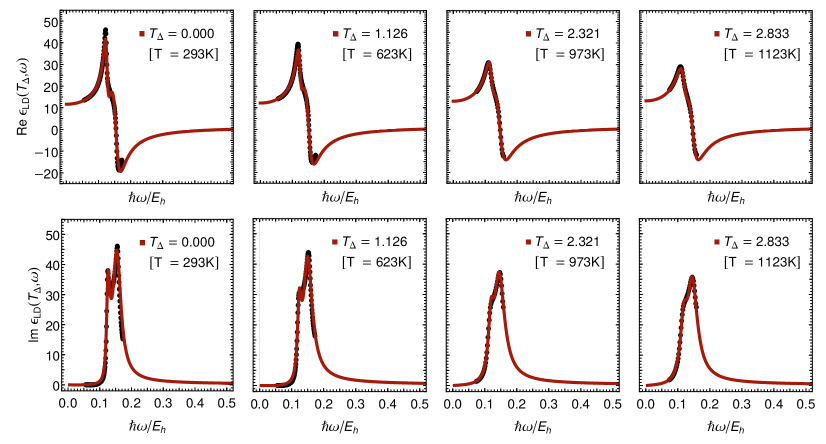
Figure 3: We present the analog of Fig. 1 for the LD as opposed to the CM fitting procedure. Again, real (top row) and imaginary (bottom row) parts of the dielectric function $\epsilon_{\mathrm{LD}}(T_{\Delta},\omega)$ are plotted as functions of frequency $\omega$, for monocrystalline silicon for various temperatures, but here, for the LD fitting procedure. Experimental data [23, 13] (dotted) are found to be in agreement with the LD fit (red) defined in Eq. (5) for temperature-dependent parameters given in Eq. (15) and coefficients in Table 6. For the LD fit, eight additional temperatures, between $T_{\Delta}=0$ and $T_{\Delta}=2.83$, namely, the values $T_{\Delta}=0.273$, $0.444$, $0.614$, $0.785$, $1.126$, $1.297$, $1.468$, and $1.638$, are considered in Ref. [45].

II.3 Lorentz-Dirac Model

As discussed in Sec. II.1, we now turn to the second method of fitting the dielectric function of the reference substrate, monocrystalline silicon, which is based on a direct fit of the experimentally determined dielectric function $\epsilon(T_{\Delta},\omega)$ to the Lorentz-Dirac master function Eq. (1) with free parameters. We introduce a phenomenological description of the dielectric function by assuming a temperature dependence of the individual parameters, and write the temperature-dependent dielectric function in terms of a functional form inspired by the master function given in Eq. (1), but with temperature-dependent parameters,

$$\epsilon(T_{\Delta},\omega)\approx\epsilon_{\mathrm{LD}}(T_{\Delta},\omega)=1\\ +\sum_{k=1}^{k_{\rm max}}\frac{a^{\mathrm{LD}}_{k}(T_{\Delta})\,\left\{[\,\omega^{\mathrm{LD}}_{k}(T_{\Delta})\,]^{2}-\mathrm{i}\,\gamma^{\prime\mathrm{LD}}_{k}(T_{\Delta})\,\omega\right\}}{[\,\omega^{\mathrm{LD}}_{k}(T_{\Delta})\,]^{2}-\omega^{2}-\mathrm{i}\,\omega\,\gamma^{\mathrm{LD}}_{k}(T_{\Delta})}\,,$$ (12)

where we employ a fitting procedure during the step that is marked with the $\approx$ sign. The temperature-dependent real part of $\epsilon(T_{\Delta},\omega)$ can thus be written as follows,

$$\mathrm{Re}[\epsilon_{\mathrm{LD}}(T_{\Delta},\omega)]=1+\sum_{k=1}^{k_{\rm max}}a^{\mathrm{LD}}_{k}(T_{\Delta})\\ \times\frac{\omega^{2}\left[\,\gamma^{\mathrm{LD}}_{k}(T_{\Delta})\,\gamma_{k}^{\prime\mathrm{LD}}(T_{\Delta})-\omega^{\mathrm{LD}}_{k}(T_{\Delta})^{2}\,\right]+\omega^{4}}{(\omega^{2}-[\omega^{\mathrm{LD}}_{k}(T_{\Delta})]^{2})^{2}+\omega^{2}\,\left[\gamma^{\mathrm{LD}}_{k}(T_{\Delta})\right]^{2}}\,.$$ (13)

The imaginary part is given as follows,

$$\mathrm{Im}[\epsilon_{\mathrm{LD}}(T_{\Delta},\omega)]=\sum_{k=1}^{k_{\rm max}}a^{\mathrm{LD}}_{k}(T_{\Delta})\,\omega\\ \times\frac{\omega^{2}\gamma_{k}^{\prime\mathrm{LD}}(T_{\Delta})+\left\{\gamma^{\mathrm{LD}}_{k}(T_{\Delta})-\gamma_{k}^{\prime\mathrm{LD}}(T_{\Delta})\right\}[\omega^{\mathrm{LD}}_{k}(T_{\Delta})]^{2}}{\{\omega^{2}-[\omega_{k}(T_{\Delta})]^{2}\}^{2}+\omega^{2}\,\left[\,\gamma^{\mathrm{LD}}_{k}(T_{\Delta})\,\right]^{2}}.$$ (14)

In full analogy with the approach outlined in Refs. [5, 4] and in Sec. II.2 [see Eq. (11)], the coefficients $a_{k}(T_{\Delta})$, $\omega_{k}(T_{\Delta})$, and $\gamma_{k}(T_{\Delta})$ are approximated by quadratic functions in the temperature,

$$a_{k}(T_{\Delta})= \;a^{\mathrm{LD}}_{k,0}+a^{\mathrm{LD}}_{k,1}\;T_{\Delta}+a^{\mathrm{LD}}_{k,2}\;(T_{\Delta})^{2}\,,$$ (15a)

$$\omega_{k}(T_{\Delta})= \;\omega^{\mathrm{LD}}_{k,0}+\omega^{\mathrm{LD}}_{k,1}\;T_{\Delta}+\omega^{\mathrm{LD}}_{k,2}\;(T_{\Delta})^{2}\,,$$ (15b)

$$\gamma_{k}(T_{\Delta})= \;\gamma^{\mathrm{LD}}_{k,0}+\gamma^{\mathrm{LD}}_{k,1}\;T_{\Delta}+\gamma^{\mathrm{LD}}_{k,2}\;(T_{\Delta})^{2}\,,$$ (15c)

$$\gamma_{k}^{\prime}(T_{\Delta})= \;\gamma^{\prime\mathrm{LD}}_{k,0}+\gamma^{\prime\mathrm{LD}}_{k,1}\;T_{\Delta}+\gamma^{\prime\mathrm{LD}}_{k,2}\;(T_{\Delta})^{2}\,,$$ (15d)

where $T_{0}=293$K. In Tables 4 and 5, we show the Clausius-Mossotti dielectric ratio coefficients for intrinsic silicon, obtained by fitting data taken from Refs. [14, 19] to Eqs. (13) and (14), for the first two resonances. Coefficients from Tables 4 and 5 are then fitted by assuming a quadratic temperature dependence according to Eq. (15), to obtain the dielectric function for silicon $\epsilon(T_{\Delta},\omega)$ as a function of temperature and driving frequency. The coefficients from this fit are given in Table 6. The accuracy of the fits can be seen in Fig. 3 where the LD fit defined in Eq. (5) is plotted alongside experimental data[14, 19], using the coefficients from Table 6 and temperature-dependent parameters given in Eq. (15). The similarity of the plots given in Fig. 3 to those in Fig. 1 reveals that the CM fitting and the LD fitting both accurately reproduce the experimental data using different methods. A unified three-dimensional representation for the dielectric function of silicon is given in Fig. 4.

For the LD fits, one particular point is worth mentioning: If one searches for the best fit parameters (in the sense of a least-squares approach) for the fitting procedure $\epsilon_{\mathrm{LD}}(T_{\Delta},\omega)\doteq 1+f(T_{\Delta},\omega)$, with unrestricted fit parameters $a_{k}$, $\omega_{k}$, $\gamma_{k}$, and $\gamma^{\prime}_{k}$, then one may incur, for certain temperatures, fitting functions for $\epsilon_{\mathrm{LD}}(T_{\Delta},\omega)$ whose imaginary part, for small and positive $\omega$, turns slightly negative. This behavior is unphysical. We have therefore implemented the condition

$$\left.\frac{\partial}{\partial\omega}\mathrm{Im}[\epsilon_{\mathrm{LD}}(T_{\Delta},\omega)]\right|_{\omega=0}=\\ \sum_{k=1}^{k_{\rm max}}\frac{a^{\mathrm{LD}}_{k}(T_{\Delta})}{[\omega^{\mathrm{LD}}_{k}(T_{\Delta})]^{2}}\left(\gamma_{k}^{\mathrm{LD}}(T_{\Delta})-\gamma^{\prime\mathrm{LD}}_{k}(T_{\Delta})\right)\;>\;0$$ (16)

in the nonlinear fitting procedure [52] via additional derivatives. We observe that, as we ensure that the first derivative of the fitted imaginary part at zero frequency is forced to be positive, the entire fitted imaginary part consistently assumes positive values over the entire frequency range $0<\omega<\infty$.

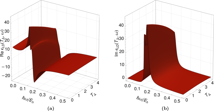
Figure 4: We present the analog of Fig. 2 for the LD fit, as opposed to the CM fit of the dielectric function. Real (a) and imaginary (b) parts of the dielectric function $\epsilon_{\mathrm{LD}}(T_{\Delta},\omega)$, as described by Eq. (5), are plotted as functions of the reduced temperature $T_{\Delta}$ and driving frequency $\omega$, for monocrystalline silicon with parameters given in Eq. (15) and coefficients in Table 6. We find good agreement of the LD fit shown here and the CM fit shown in Fig. 2.

Table 7: Short-distance coupling parameters $C_{3}^{\mathrm{CM}}$ and $C_{3}^{\mathrm{LD}}$ of the Casimir-Polder potential are given for helium interacting with a monocrystalline silicon surface. Results are given for the CM and the LD fitting procedures given in Eqs. (4) and Eq. (5), respectively. The numerical values are obtained using the integrals given in Eqs. (19) and (20). The data is plotted in Fig. 5, as a function of the temperature.

Helium on Silicon
Short-Range $C_{3}$ Coefficient
$T_{\Delta}$	$C_{3}^{\mathrm{CM}}$ [$a_{0}^{3}E_{h}$]	$C_{3}^{\mathrm{LD}}$ [$a_{0}^{3}E_{h}$]	$\%$ difference
0.000	0.04906	0.04950	0.91
0.273	0.05013	0.05068	1.10
0.444	0.05128	0.05132	0.08
0.614	0.05143	0.05173	0.57
0.785	0.05198	0.05253	1.04
0.956	0.05247	0.05276	0.54
1.126	0.05295	0.05297	0.04
1.297	0.05321	0.05311	0.18
1.468	0.05376	0.05317	1.09
1.638	0.05254	0.05274	0.38
2.321	0.05066	0.05123	1.13
2.833	0.05022	0.05021	0.03

Table 8: Long-distance coupling parameters $C_{4}^{\mathrm{CM}}$ and $C_{4}^{\mathrm{LD}}$ of the Casimir-Polder potential are given for helium interacting with a monocrystalline silicon surface. Results are given for the CM and the LD fitting procedures given in Eqs. (4) and Eq. (5), respectively. Values are compared with Eqs. (26) and (27) in Fig. 6.

Helium on Silicon
Long-Range $C_{4}$ Coefficient
$T_{\Delta}$	$C_{4}^{\mathrm{CM}}$ [$a_{0}^{4}E_{h}$]	$C_{4}^{\mathrm{LD}}$ [$a_{0}^{4}E_{h}$]	$\%$ difference
0.000	15.32	15.40	0.55
0.273	15.37	15.49	0.76
0.444	15.41	15.50	0.61
0.614	15.42	15.55	0.82
0.785	15.44	15.57	0.84
0.956	15.45	15.56	0.70
1.126	15.47	15.55	0.51
1.297	15.49	15.60	0.70
1.468	15.52	15.62	0.63
1.638	15.59	15.69	0.65
2.321	15.67	15.78	0.69
2.833	15.83	15.82	0.04

III Atom-Surface Potentials

The transition of the atom-surface potential from the short-range to the long-range region has been discussed at length in the literature (see, e.g., Refs. [53, 54, 55, 49] and references therein). It is well known that the atom-surface potentials $V(z)$ mediated by the exchange of virtual photons change from a $1/z^{3}$ short-range asymptotic behavior to a $1/z^{4}$ long-range asymptotic behavior ($z$ is the atom-wall distance). The $1/z^{3}$ short-range asymptotic behavior persists for $z\ll a_{0}/\alpha$, while the $1/z^{4}$ long-range asymptotic behavior is relevant for long range, $z\gg a_{0}/\alpha$, where $a_{0}$ is the Bohr radius and $\alpha$ is the fine-structure constant. The asymptotic forms are

$$V(z)= \;-\frac{C_{3}}{z^{3}}=-(C_{3})_{\mathrm{a.u.}}\;\frac{E_{h}}{(z/a_{0})^{3}}\,,\quad a_{0}\ll z\ll\frac{a_{0}}{\alpha}\,,$$ (17a)

$$V(z)= \;-\frac{C_{4}}{z^{4}}=-(C_{4})_{\mathrm{a.u.}}\;\frac{E_{h}}{(z/a_{0})^{4}}\,,\quad z\gg\frac{a_{0}}{\alpha}\,.$$ (17b)

Here, we denote the numerical value of the $C_{3}$ and $C_{4}$ coefficients, measured in atomic units, by $(C_{3})_{\mathrm{a.u.}}$ and $(C_{4})_{\mathrm{a.u.}}$, respectively.

The $C_{3}$ and $C_{4}$ coefficients are, in a natural way, temperature-dependent, as they depend on the dielectric function of the substrate material [54, 56, 57, 58]. Hence, there is a functional relationship $C_{3}=C_{3}(T_{\Delta})$ and $C_{4}=C_{4}(T_{\Delta})$. It is thus clear that, for atom-surface interaction studies, it is convenient to have analytic models for the temperature-dependent dielectric function of a material; we here consider the case of intrinsic silicon. The temperature dependence of the coefficient $C_{3}(T_{\Delta})$, which governs the short-distance behavior of the Casimir-Polder potential, can be written as follows [53, 54, 55, 49],

$$C_{3}(T_{\Delta})=\frac{\hbar}{16\pi^{2}\epsilon_{0}}\int_{0}^{\infty}\mathrm{d}\omega\;\alpha(\mathrm{i}\omega)\;\frac{\epsilon(T_{\Delta},\mathrm{i}\omega)-1}{\epsilon(T_{\Delta},\mathrm{i}\omega)+1}\,.$$ (18)

Based on the two fitting procedures given in Eqs. (8) and (12), we can define the coefficients

$$C^{\mathrm{CM}}_{3}(T_{\Delta})= \;\frac{\hbar}{16\pi^{2}\epsilon_{0}}\int_{0}^{\infty}\mathrm{d}\omega\;\alpha(\mathrm{i}\omega)\;\frac{\epsilon_{\mathrm{CM}}(T_{\Delta},\mathrm{i}\omega)-1}{\epsilon_{\mathrm{CM}}(T_{\Delta},\mathrm{i}\omega)+1}\,,$$ (19)

for the Clausius-Mossotti fit, and analogously

$$C^{\mathrm{LD}}_{3}(T_{\Delta})= \;\frac{\hbar}{16\pi^{2}\epsilon_{0}}\int_{0}^{\infty}\mathrm{d}\omega\;\alpha(\mathrm{i}\omega)\;\frac{\epsilon_{\mathrm{LD}}(T_{\Delta},\mathrm{i}\omega)-1}{\epsilon_{\mathrm{LD}}(T_{\Delta},\mathrm{i}\omega)+1}$$ (20)

for the Lorentz-Dirac fit. In order to calculate $C_{3}(T_{\Delta})$, we need the dynamic polarizability of the atom $\alpha(\omega)$. In Appendix B, we describe a rather universally applicable scheme for the calculation of the dynamic polarizability of an arbitrary atom, based on tabulated oscillator strength for a limited set of transitions, augmented by a matching (at high energy) against the Thomas-Reiche-Kuhn (TRK) sum rule [59, 60]. The method uses the fact that, at a purely imaginary argument, the dynamic polarizability is a smooth function which avoids the singularities of the integrand at the resonance frequencies. We have applied the method to both atomic hydrogen as well as helium, neon, argon, krypton and xenon. For helium interacting with a silicon surface, results are given in Table 7. Results for helium interacting with silicon are also shown in Fig. 5. A remark is in order. The numerical results given in Table 7 correspond to the parameter fits for individual temperatures, as outlined in Eqs. (4) and Eq. (5), and in Tables 1 and 2. The smooth curves in Fig. 5 (and analogously in Fig. 6) constitute the results of plotting Eqs. (4) and Eq. (5) using the smooth temperature-dependent model outlined in the coefficients given in Tables 3 and 4. For room temperature, these are in agreement with those recently presented in Ref. [61]. A separate least-squares fit using a quadratic polynomial in $T_{\Delta}$ yields the following result for the temperature-dependent $C_{3}$ coefficients for helium on silicon,

$$C^{\mathrm{CM}}_{3}(T_{\Delta})\approx \;C^{\mathrm{CM}}_{3}(0)\,\left\{1+c_{\rm CM}\,T_{\Delta}+d_{\rm CM}(T_{\Delta})^{2}\right\}\,,$$ (21)

where $C^{\mathrm{CM}}_{3}(0)=0.04905$, $c_{\rm CM}=0.10569$, and $d_{\rm CM}=-0.034338$. Analogously, one obtains

$$C^{\mathrm{LD}}_{3}(T_{\Delta})\approx \;C^{\mathrm{LD}}_{3}(0)\,\left\{1+c_{\rm LD}T_{\Delta}+d_{\rm LD}(T_{\Delta})^{2}\right\}\,,$$ (22)

where $C^{\mathrm{LD}}_{3}(0)=0.04923$, $c_{\rm LD}=0.09939$, and $d_{\rm LD}=-0.033309$.

For the other atoms under investigation, the $C_{3}$ coefficient read as follows. For H, we obtain, using the Lorentz-Dirac fit, in atomic units, at room temperature, a result of $0.1042$, while for Ne, Ar, Kr, and Xe, the results for $C_{3}$, in atomic units, read as $0.1080$, $0.3914$, $0.5853$ and $0.9157$, respectively.

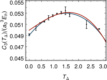
Figure 5: Short-distance coupling parameters $C_{3}^{\mathrm{CM}}(T_{\Delta})$ and $C_{3}^{\mathrm{LD}}(T_{\Delta})$ of the Casimir-Polder potential, are plotted as functions of $T_{\Delta}$ for helium interacting with a monocrystalline silicon surface. Data points (black dots) are taken from Table 7. The blue curve corresponds to the Clausius-Mossotti fit, given in Eq. (19), while the red curve corresponds to the Lorentz-Dirac fit, given in Eq. (20). The data points are taken at $T_{\Delta}=0.000$, $0.273$, $0.444$, $0.614$, $0.785$, $0.956$, $1.126$, $1.297$, $1.468$, $1.638$, $2.321$, and $2.833$.

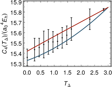
Figure 6: Long-distance coupling parameters $C_{4}^{\mathrm{CM}}(T_{\Delta})$ and $C_{4}^{\mathrm{LD}}(T_{\Delta})$ of the Casimir-Polder potential, are plotted as functions of $T_{\Delta}$ for helium interacting with a monocrystalline silicon surface . Data points (black dots) are taken from Table 8. The blue curve corresponds to the Clausius-Mossotti fit, given in Eq. (26), while the red curve corresponds to the Lorentz-Dirac fit, given in Eq. (27). The data points are taken at $T_{\Delta}=0.000$, $0.273$, $0.444$, $0.614$, $0.785$, $0.956$, $1.126$, $1.297$, $1.468$, $1.638$, $2.321$, and $2.833$.

Let us now investigate the long-range asymptotic behavior, as described by Eq. (17b), and let us consider the temperature dependence of the $C_{4}$ long-range coefficient. Indeed, the $C_{4}$ coefficient governing the long-distance behavior $z\gg a_{0}/\alpha$ of the Casimir-Polder potential can be written as [53, 54, 49]

$$C_{4}(T_{\Delta})=\frac{\hbar c}{2\pi}\frac{3}{8}\;\alpha(0)\;\phi(T_{\Delta})\,,$$ (23)

where $\alpha(0)=\alpha(\omega=0)$ is the static polarizability of the atom. The emergence of $\alpha(0)$ in the result illustrates the fact that, for large atom-wall separation, the interaction is mediated by very low-energy virtual photons. The $\phi$ function in Eq. (23) is given as an integral, as follows,

$$\phi(T_{\Delta})=\int_{1}^{\infty}\mathrm{d}p\,\frac{H(\epsilon(T_{\Delta},0),p)}{p^{4}}\,,$$ (24)

where the $H$ function reads [53, 54, 49]

$$H(\epsilon,p)=\frac{\sqrt{\epsilon-1+p^{2}}-p}{\sqrt{\epsilon-1+p^{2}}+p}+(1-2p^{2})\frac{\sqrt{\epsilon-1+p^{2}}-p\,\epsilon}{\sqrt{\epsilon-1+p^{2}}+p\,\epsilon}.$$ (25)

The $C_{4}$ coefficient can be calculated on the basis of the Clausius-Mossotti fit described in Sec. II.2,

$$C^{\mathrm{CM}}_{4}(T_{\Delta})= \;\frac{\hbar c}{2\pi}\frac{3}{8}\alpha(0)\;\phi_{\mathrm{CM}}(T_{\Delta})\,,$$ (26a)

$$\phi_{\mathrm{CM}}(T_{\Delta})= \;\int_{1}^{\infty}\mathrm{d}p\,\frac{H(\epsilon_{\mathrm{CM}}(T_{\Delta},0),p)}{p^{4}}\,,$$ (26b)

or the Lorentz-Dirac fit, described in Sec. II.3,

$$C_{4}^{\mathrm{LD}}(T_{\Delta})= \;\frac{\hbar c}{2\pi}\frac{3}{8}\alpha(0)\;\phi_{\mathrm{LD}}(T_{\Delta})\,,$$ (27a)

$$\phi_{\mathrm{LD}}(T_{\Delta})= \;\int_{1}^{\infty}\mathrm{d}p\,\frac{H(\epsilon_{\mathrm{LD}}(T_{\Delta},0),p)}{p^{4}}\,.$$ (27b)

An analytic result for $\phi$, expressed with logarithms, reads as follows,

$$\phi(T_{\Delta})=2\left[\frac{2\epsilon(T_{\Delta},0)^{3}-4\epsilon(T_{\Delta},0)^{2}+3\epsilon(T_{\Delta},0)+1}{4(\epsilon(T_{\Delta},0)-1)^{3/2}}L_{1}\right.\\[0.4878pt] +\frac{\epsilon(T_{\Delta},0)^{2}}{2\sqrt{\epsilon(T_{\Delta},0)+1}}\,\left\{L_{2}-L_{3}\right\}+\frac{1}{6(\epsilon(T_{\Delta},0)-1)}\bigl{[}6\epsilon(T_{\Delta},0)^{2}\\[0.4878pt] \left.-3\epsilon(T_{\Delta},0)^{3/2}-4\epsilon(T_{\Delta},0)-3\sqrt{\epsilon(T_{\Delta},0)}+10\bigr{]}\right]\,.$$ (28)

Here, the logarithmic terms are

$$L_{1}= \;\ln\left(\frac{\sqrt{\epsilon(T_{\Delta},0)}-\sqrt{\epsilon(T_{\Delta},0)-1}}{\sqrt{\epsilon(T_{\Delta},0)}+\sqrt{\epsilon(T_{\Delta},0)-1}}\right)\,,$$ (29a)

$$L_{2}= \;\ln\left(\frac{\sqrt{\epsilon(T_{\Delta},0)+1}-1}{\sqrt{\epsilon(T_{\Delta},0)+1}+1}\right)\,,$$ (29b)

$$L_{3}= \;\ln\left(\frac{\sqrt{\epsilon(T_{\Delta},0)+1}-\sqrt{\epsilon(T_{\Delta},0)}}{\sqrt{\epsilon(T_{\Delta},0)+1}+\sqrt{\epsilon(T_{\Delta},0)}}\right)\,.$$ (29c)

Our result for $\phi(T_{\Delta})$ is in agreement with the result given in Eq. (23) of Ref. [54], but differs in its functional form; we attempt to reduce the complexity of the functions involved. The term in square brackets in Eq. (28) approximates unity in the limit of a perfectly conducting surface, $\epsilon(T_{\Delta},0)\to\infty$. The correction terms about the limit of large $\epsilon(T_{\Delta},0)$ can be expanded in a series in inverse half-integer powers of $\epsilon(T_{\Delta},0)$. The first two correction terms lead to the expression

$$\phi(T_{\Delta})=2\biggl{[}1-\frac{5}{4\sqrt{\epsilon(T_{\Delta},0)}}\\[0.4878pt] +\frac{22}{15\epsilon(T_{\Delta},0)}+\mathcal{O}\left(\frac{\ln[\epsilon(T_{\Delta},0)]}{\epsilon(T_{\Delta},0)^{3/2}}\right)\biggr{]}\,.$$ (30)

Numerical values for $C_{4}(T_{\Delta})$ are calculated for each value of $T_{\Delta}$, for both the CM fitting procedure [according to Eq. (26)] and the LD fitting method [according to Eq. (27)]. Results for helium atoms interacting with a silicon surface are given in Table 8 and Fig. 6.

Conversely, a fit using a quadratic polynomial in $T_{\Delta}$ yields the following result for the temperature-dependent $C_{4}$ coefficients for helium on silicon,

$$C^{\mathrm{CM}}_{4}(T_{\Delta})\approx \;C^{\mathrm{CM}}_{4}(0)\,\left\{1+f_{\rm CM}\,T_{\Delta}+g_{\rm CM}(T_{\Delta})^{2}\right\}\,,$$ (31)

where $C^{\mathrm{CM}}_{4}(0)=15.32$, $f_{\rm CM}=0.0076444$, and $g_{\rm CM}=0.0014732$. Analogously, one obtains

$$C^{\mathrm{LD}}_{4}(T_{\Delta})\approx \;C^{\mathrm{LD}}_{4}(0)\,\left\{1+f_{\rm LD}T_{\Delta}+g_{\rm LD}(T_{\Delta})^{2}\right\}\,,$$ (32)

where $C^{\mathrm{LD}}_{4}(0)=15.40$, $f_{\rm LD}=0.013560$, and $g_{\rm LD}=-0.0013667$.

The relative discrepancies between the CM and LD fits for $C_{4}$ are commensurate with those for the corresponding $C_{3}$ coefficients, as listed in Tables 7 and 8. This is consistent with fact that the $C_{4}$ coefficients are determined by the static value $\epsilon(T_{\Delta},\omega=0)$ of the dielectric function, which can be determined to roughly the same accuracy as the integral over all frequencies, which enters Eq. (18). Note, also, that the static value of the helium polarizability is well known from Refs. [62, 63]. A further remark might be in order. The relative difference of the numerical values for the $C_{4}$ coefficients, obtained from the CM and LD fits, is smaller by about a factor of five than the relative difference of the static dielectric function $\epsilon(T_{\Delta},0)$, obtained from either fit. This somewhat surprising observation finds a natural explanation when one considers the numerically small variation of the $\phi$ function with respect to the value of $\epsilon(T_{\Delta},0)$, in the relevant range $\epsilon(T_{\Delta},0)\approx 11.5$. In consequence, the $C_{4}$ coefficients are determined to much better accuracy than the static dielectric function.

For the other atoms under investigation, the $C_{4}$ coefficient read as follows. For H, Ne, Ar, Kr, and Xe, the results for $C_{4}$, in atomic units, read as $49.99$, $29.52$, $122.9$, $182.8$ and $303.0$, respectively (at room temperature).

IV Conclusions

We have found a unified description of the temperature-dependent and frequency-dependent dielectric function $\epsilon(T_{\Delta},\omega)$ of intrinsic (monocrystalline) silicon, using the LD and CM functional forms, augmented by radiation-reaction terms, with only two generalized oscillator terms entering the master function given in Eq. (1). For intrinsic silicon, we find that both the CM function $[\epsilon(\omega)-1]/[\epsilon(\omega)+2]$ as well as the LD function $[\epsilon(\omega)-1]$ itself can be fitted very well to experimental data. This conclusion is fully consistent with the observations made in Ref. [27], where a model without radiation reaction was considered. The $R^{2}$ values are greater than $0.99$ for either fit, for all temperatures studied here, as evident from Fig. 2 of Ref. [45]. The CM fit is able to represent experimental data marginally better than the LD fit, consistent with its ability to model the local-field effect. The temperature-dependence of the coefficients of our model is well described by simple quadratic forms.

Our fitting, as described in Secs. II.1 and II.2, is successful, and leads to the temperature-dependent parameters listed in Tables 3 and 6. These lead to a satisfactory representation of the dielectric function of intrinsic silicon in the temperature range $0<T_{\Delta}<2.83$, i.e., $293\,{\rm K}<T<1123\,{\rm K}$. The entire problem is of considerable interest, and the investigation of a uniform representation of the dielectric function over a wide temperature range requires a careful evaluation of available experimental data (see Appendix A.1). The fact that a unified model with analytic coefficients is able to describe the temperature-dependent, and frequency-dependent dielectric function of intrinsic silicon over wide ranges of the parameters, could be interpreted as supporting the self-consistency of the experimental data for the dielectric function, obtained by various different groups over the past two decades [13, 14, 19, 20, 23].

We employ the results of our fitting in the temperature-dependent evaluation of the short-range, and long-range, asymptotics of the atom-surface interaction potential for helium atoms interacting with intrinsic silicon (see Sec. III). We find that the $C_{3}$ and $C_{4}$ coefficients given in Eqs. (17a) and (17b) exhibit a moderate temperature dependence depicted in Figs. 5 and 6. Our approach allows us to determine temperature-dependence $C_{3}$ and $C_{4}$ coefficients with a relative accuracy which we would like to conservatively estimate as 5%, due to the intrinsic uncertainty in the experimental data, even if the relative difference of the $C_{3}$ and $C_{4}$ coefficients given in Tables 7 and 8 is smaller than 5%. This estimate is supported by an error propagation calculation based on computer algebra [52], which propagates the uncertainty estimate for the fit parameters given in Ref. [45] to the determination of the $C_{3}$ and $C_{4}$ coefficients. Interestingly, our calculations imply the existence of a manifest temperature dependence of atom-surface interactions, which goes beyond the “thermal discretization” of the frequencies of the virtual photons that mediate the atom-surface interaction, in terms of the Matsubara frequencies [64, DzLiPi1961spu, 65].

Appendix A Intricacies of the Dielectric Function

A.1 Brief Review of Published Data

A very brief review of the available experimental data for the dielectric function of intrinsic silicon might be in order. The subject is interesting because of a significant dependence on the sample preparation, with tiny surface impurities having a potentially detrimental effect on the accuracy of the obtained data. In view of apparent discrepancies among some published data, which will be discussed in the following, we here prefer to use rather recent compilations of optical properties of silicon; it is hoped that potential issues with previous measurements may have been addressed in the more recent compilations. Specifically, our sources for experimental data of silicon at room temperature are Refs. [13, 20, 23]. Our main sources of temperature-dependent data are Refs. [14, 19]. We use Ref. [19] as a source for the experimental measurements of silicon at $298$ K, $523$ K, $773$ K, $973$ K, and $1123$ K. For completeness, Ref. [14] is used as a source for experimental measurements of silicon at $293$ K (additional data for room temperature), $373$ K, $423$ K, $473$ K, $523$ K, $573$ K, $623$ K, $723$ K. As a side remark, we can add that the room temperature data ($293$ K, from Refs. [13, 14, 20, 23]) differ only very slightly from the data obtained for $298$ K in Ref. [19]. The data for $298$ K cover a smaller frequency range as compared to the data for $293$ K; the discussion of the data available for $298$ K is relegated to Ref. [45]. We also mention Ref. [20] for a discussion of the temperature dependence of the dielectric function of silicon, where the linear term of the coefficients (as a function of the temperature $T$) is taken into account.

Now, for completeness, let us briefly discuss some apparent discrepancies among other data sets. For example, in Ref. [16], it is pointed out that “recent measurements [13, 17], at both the ultraviolet and infrared ends of the spectrum have considerably improved the accuracy of silicon optical data at these wavelengths, rendering past tabulations [8, 9, 10] and assessments [15] largely obsolete.” Along the same direction, in Sec. IV.b of Ref. [18], it is pointed out that the compilation of silicon (Si) optical data in Ref. [8] relies on two sets of silicon absorption values based on the intensity transmission measurements originally reported in Refs. [3, 1]. Yet, it is pointed out in Sec. IV.b of Ref. [18], that the values reported in Ref. [3] spanning 1.2-2 eV were obtained from very thin epitaxial films on sapphire and there is a mismatch by a factor of 5 at 1.28 eV as compared to the values reported in Ref. [1].

In Ref. [18], near the start in the Introduction, it is pointed out that: “However, even though silicon is one of the most heavily studied and well-understood materials, the accuracy of reported optical constant spectra for crystalline silicon is still an issue. The original spectroscopic ellipsometry results for silicon obtained by Aspnes [7] have been questioned (especially for energies less than 3.4 eV by the work of Jellison [13] using a two-channel polarization modulation ellipsometer).” Furthermore, in Ref. [18], near the start in the Introduction, it is also pointed out that the measurements reported in Ref. [7] were complicated both by the difficulty of stripping residual oxide without roughening the sample and by acquisition of ellipsometric data at an angle of incidence which pushed the measured ellipsometric values at smaller photon energies into a sub-optimal region for the rotating-analyzer ellipsometer (RAE) used. It is also pointed out that in Ref. [13], a careful oxide layer removal procedure was profiting from a separate intensity transmission measurement used in order to establish the overlayer thickness.

Finally, we should also mention that we have made several unsuccessful attempts to fit the data given in Ref. [8] over the frequency range $0<\hbar\omega<5\,{\rm eV}$ with functional forms that fulfill the Kramers-Kronig relations. An inspection reveals that data for the imaginary part of the dielectric function given in Ref. [11], and Refs. [14, 19], exceeds the values given in Ref. [8] in the frequency range $1<\hbar\omega<2\,{\rm eV}$ by almost a factor two. The newer data given in Refs. [14, 19] is amenable to a fit using a consistent functional form, as detailed in this current study. Furthermore, we note that no actual data pairs of frequency and real and imaginary part of the dielectric function are given in Ref. [11]. However, a quantitative inspection of the curves given Figs. 2, 3, and 4 of Ref. [11] leads to the conclusion that the data on which the Ref. [11] is based, are in agreement with the analysis presented in the current investigation.

The availability of convenient, consistent, simple functional forms to describe the frequency-dependent, and temperature-dependent dielectric function of intrinsic silicon, as derived here, should thus be of considerable interest to the community.

A.2 Lorentz-Dirac Model

Let us start from Eq. (2) Ref. [22], which describes the acceleration $\vec{a}$ on a charge carrier particle of charge $q$ in terms of the Lorentz-Dirac formalism,

$$\vec{a}=\frac{1}{m}\vec{F}_{\rm ext}+t_{0}\,\dot{\vec{a}}\,.$$ (33)

The latter term describes radiation reaction. A discussion of the Lorentz-Dirac equation can be found in Sec. 8.6.2 of Ref. [26]. The radiation reaction time is [see Eq. (3) of Ref. [22]]

$$t_{0}=\frac{q^{2}}{6\pi\epsilon_{0}mc^{3}}\,.$$ (34)

One defines a characteristic acceleration $\vec{a}_{c}$ and a characteristic time scale $t_{c}$ through the formulas [see Eqs. (4) and (5) of Ref. [22]]

$$\vec{a}_{c}=\frac{1}{m}\,\vec{F}_{\rm ext}\,,\qquad\dot{\vec{a}}_{c}=\frac{\vec{a}_{c}}{t_{c}}\,,$$ (35)

where $\vec{F}_{\rm ext}$ is the external force. Then, according to Eq. (6) of Ref. [22], one defines

$$t_{\rm light}=s_{q}/c$$ (36)

as the time it takes light to travel a characteristic distance $s_{q}$ which could be chosen as the size of the charge distribution, or, from a classical point of view, as the classical electron radius obtained by equating the electron rest mass with the electrostatic self-energy of the electron’s charge distribution, taken as centered on a sphere of radius $s_{q}$. Then, according to Eq. (7) of Ref. [22], one has

$$m\sim m_{\rm em}\sim\frac{q^{2}}{4\pi\epsilon_{0}s_{q}}\,,$$ (37)

where $m_{\rm em}$ is the self-energy (self-mass) of the electron.

One assumes a not-too-fast change in the acceleration, i.e., a not-too-abrupt dynamical change,

$$t_{c}\gg t_{\rm light}\,.$$ (38)

Under the observation [see Eq. (9) of Ref. [22]] that $t_{0}\sim t_{\rm light}$, one derives the condition [see Eq. (10) of Ref. [22]]

$$t_{0}\sim t_{\rm light}\ll t_{c}\,,\qquad t_{0}/t_{c}\ll 1\,,$$ (39)

under which the authors of Ref. [22] arrive at the following formula [see Eq. (25) of Ref. [22]] for the polarization density $\vec{P}$ in the sample,

$$\frac{\mathrm{d}^{2}\vec{P}}{\mathrm{d}t^{2}}+\left(2\Gamma+t_{0}\,\omega_{r}^{2}-\frac{q^{2}t_{0}N}{3m\epsilon_{0}}\right)\,\frac{\mathrm{d}\vec{P}}{\mathrm{d}t}\\ +\left(\omega_{r}^{2}-\frac{q^{2}N}{3m\epsilon_{0}}\right)\vec{P}=\frac{q^{2}N}{m}\,\vec{E}+\frac{q^{2}Nt_{0}}{m}\,\frac{\mathrm{d}\vec{E}}{\mathrm{d}t}\,.$$ (40)

From Ref. [22], one can see that $\Gamma$ is the damping rate associated with the frictional force between atoms, $\omega_{r}$ is the natural frequency of the restoring force, $N$ is the number of atoms per unit volume, and $q$ is the charge of the electron. The transformation to Fourier space proceeds by writing

$$\vec{P}(t)=\int\frac{\mathrm{d}\omega}{2\pi}\,\mathrm{e}^{-\mathrm{i}\omega t}\,\vec{P}(\omega)\,,$$ (41)

so that, in Fourier space, one replaces $\mathrm{d}/\mathrm{d}t\to-\mathrm{i}\omega$.

Setting $\vec{P}(\omega)=\epsilon(\omega)\,\epsilon_{0}\,\vec{E}(\omega)$, one then arrives at the following formula,

$$\epsilon(\omega)=\epsilon_{\infty}+\frac{a_{0}-\mathrm{i}\omega\,a_{1}}{b_{0}-\omega^{2}-\mathrm{i}\omega\,b_{1}}\,.$$ (42)

With reference to Eq. (40) and Eq. (27) from Ref. [22], the parameters are identified as follows,

$$b_{1}= \;2\Gamma+t_{0}\,\omega_{r}^{2}-\frac{q^{2}t_{0}N}{3m\epsilon_{0}}\,, b_{0} =\omega_{r}^{2}-\frac{q^{2}N}{3m\epsilon_{0}}\,,$$ (43a)

$$a_{0}= \frac{q^{2}N}{m}\,, a_{1} =\frac{q^{2}t_{0}N}{m}\,.$$ (43b)

In Eq. (42), the signs of the terms multiplying $a_{1}$ and $b_{1}$ are inverted as compared to Eq. (28) of Ref. [22], presumably due to a typographical error in Ref. [22]. Note that, upon using the functional form (42), $a_{1}$ and $b_{1}$ are obtained as positive rather than negative quantities in our fitting procedure, for silicon, supporting the functional form indicated in Eq. (42) (with positive terms $a_{1}$ and $b_{1}$). This finding also is in line with the functional form used in Ref. [21].

Table 9: Energy differences are given $E_{n0}=E_{n}-E_{0}$ between the reference $1S$ ground state of hydrogen (H) and excited states (${\rm nP}$). The fine-structure and Lamb shift are not resolved. We also list corresponding oscillator strengths $f_{n0}$ for the first $10$ excited states. The data includes the reduced-mass correction (the oscillator strength scales with the first power of $\mu/m_{e}$, where $\mu$ is the reduced mass of hydrogen, and $m_{e}$ is the electron mass.) All entries are in agreement with the data compilation given in Ref. [66].

$n$	$E_{n0}\,[E_{h}]$	$f_{n0}\,[e^{2}a_{0}^{2}E_{h}]$
2	0.37480	0.41640
3	0.44421	0.07914
4	0.46850	0.02901
5	0.47974	0.01395
6	0.48585	0.00780
7	0.48954	0.00482
8	0.49193	0.00319
9	0.49356	0.00222
10	0.49473	0.00161
11	0.49560	0.00120

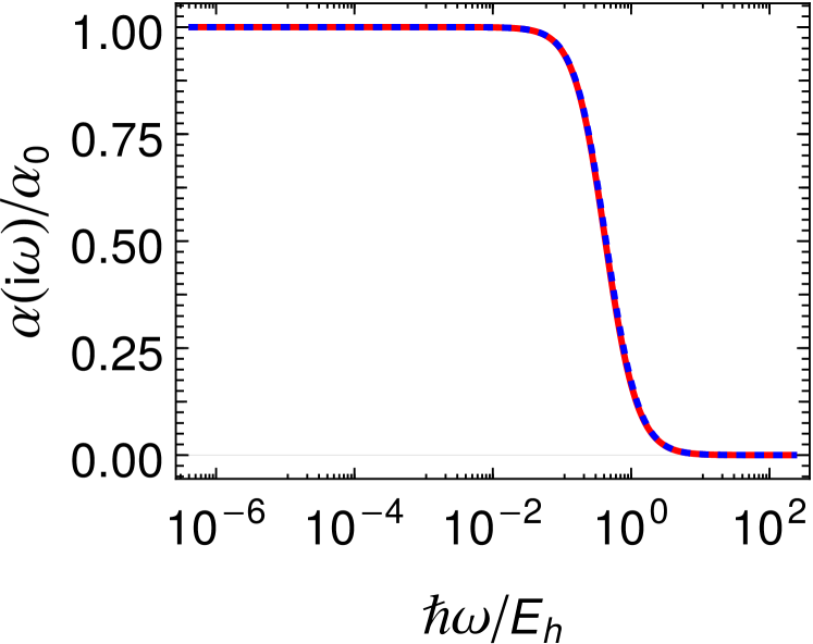
Figure 7: The dynamic polarizability of atomic hydrogen is plotted as a function of the imaginary driving frequency. The exact solution given in Eq. (51) (red curve) is compared with the approximation given in Eq. (45) (blue-dotted curve), which is based on the oscillator strengths listed in Table 9. The static polarizability of hydrogen is $\alpha_{0}=9/2e^{2}a_{0}^{2}/E_{h}$, which is $9/2$ in atomic units. The relative difference between the exact values and the approximation can be found in Fig. 8.

Figure 8: The relative difference $\chi(\omega)$, described in Eq. (56), between the exact expression for the dynamic polarizability of hydrogen given in Eq. (51) and the discrete model given in Eq. (45), is plotted as a function of the driving frequency. Here $q$ is the number of discrete oscillator strengths included in the discrete model, as given in Table 9.

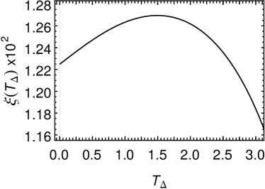
Figure 9: The relative difference $\xi(T_{\Delta})$, defined in Eq. (59), between the short-distance Casimir-Polder parameter $C_{3}$ evaluated using the exact expression for the dynamic polarizability given in Eq. (51) and the discrete model given in Eq. (45) is plotted as a function of temperature for hydrogen interacting with silicon. Note that the plot range on the ordinate axis is restricted.

Appendix B Dynamic Polarizability

B.1 General Algorithm

We aim to delineate a rather general algorithm here which allows one to calculate the dynamic polarizability of an atom at imaginary driving frequency, $\alpha(\mathrm{i}\omega)$, based on the knowledge of the oscillator strengths of a few low-lying transitions, and additional input from the known asymptotic behavior of the polarizability for large driving frequency, to be derived from sum rules. The algorithm should be accurate to a few percent over the entire frequency range $0<\omega<\infty$ and thus sufficient for the calculation of atom-surface interactions, where the dominant source of uncertainty comes from the dielectric function (see Sec. III).

The approach is to first collect, from databases [50], the transition energies and oscillator strengths of a few low-lying transitions. This collection immediately allows to describe the frequency dependence of the dynamic polarizability for low excitation frequency argument. In order to model the contribution of the continuum states of the atom, we add one more virtual transition to a “pseudo-level”, which is energetically positioned in the continuum. The oscillator strength is matched against the Thomas-Reiche-Kuhn (TRK) sum rule [59, 60] sum rule, and the energy of the pseudo-level is adjusted so that the correct overall low-frequency (“static”) limit of the polarizability is recovered. Because we only consider imaginary frequencies, we are far enough away from any atomic resonance that we do not need to worry about the decay width of the state, i.e., about the imaginary part of the energy that otherwise enters the polarizability.

The atomic polarizability is defined as (see Refs. [62, 49])

$$\alpha\left(\omega\right)=\sum_{n}^{\infty}\frac{e^{2}\,a_{0}^{2}\,E_{h}\,f_{n0}}{E_{n0}^{2}-\left(\hbar\omega\right)^{2}}\,,$$ (44)

where $f_{n0}$ is the oscillator strength of the atom, measured in atomic units, and $E_{n0}\equiv E_{n}-E_{0}$ is the energy difference between the virtual and exited states $\ket{\psi_{n}}$. We note that the oscillator strength is used, in atomic physics, as a dimensionless quantity (for an excellent overview of pertinent conventions, see Ref. [67].) The sum is carried out over all of the discrete states as well as the continuous spectrum.

In order to approximate the atomic polarizability with our model polarizability, $\alpha(\omega)\approx\alpha_{m}(\omega)$, we divide the infinite sum in Eq. (44) into two parts,

$$\alpha(\omega)\approx\alpha_{m}(\omega)=\alpha_{d}(\omega)+\alpha_{c}(\omega)\,,$$ (45)

in which $\alpha_{d}(\omega)$ is the sum over the terms from the first $q$ discrete (bound) states

$$\alpha_{d}(\omega)=\sum_{n=1}^{q}\frac{e^{2}a_{0}^{2}E_{h}\,f_{n0}}{E_{n0}^{2}-\left(\hbar\omega\right)^{2}}\,,$$ (46)

where we neglect the width of the virtual states, anticipating that our final aim will be to evaluate the polarizability at imaginary driving frequency (where the decay width terms are negligible for our purposes).

Let us denote by $\alpha_{c}$ the contribution of the continuum states. We model the contribution $\alpha_{c}(\omega)$, using a pseudo-level, as follows,

$$\alpha_{\mathrm{c}}(\omega)=\frac{e^{2}a_{0}^{2}E_{h}\,f_{\infty}}{E_{\infty}^{2}-\left(\hbar\omega\right)^{2}}\,.$$ (47)

The oscillator strength of the additional “continuum” level $f_{\infty}$ is found by requiring that sum over all oscillator strengths obey the TRK sum rule which in SI mksA units can be expressed as

$$\sum_{n}f_{n0}=N\,,$$ (48)

where $N$ is the total number of electrons in the system, and $n$ runs over all virtual levels (discrete and continuum). Therefore, the matching condition for the oscillator strength of the continuum pseudo-level is

$$f_{\infty}\approx N-\sum_{n=1}^{q}f_{n0}\,.$$ (49)

The energy position of the additional “continuum” level $E_{\infty}$ can be found by requiring our ansatz to reproduce known numerical values of the static polarizability,

$$E_{\infty}^{2}=\frac{f_{\infty}}{\alpha(0)-\alpha_{\mathrm{q}}(0)}\,.$$ (50)

This algorithm will be applied to hydrogen, before being generalized to other atoms.

B.2 Hydrogen

Because the dynamic polarizability of hydrogen can be calculated analytically [68, 69, 70, 71], a comparison of the complete result to that found using the algorithm described above can be used as a measure of the validity of our ansatz. We start from the analytic solution for the dielectric function for the ground state of hydrogen as a function of $\omega$ as described in Refs. [70, 71, 68],

$$\alpha(\omega)=\frac{e^{2}\,\hbar^{2}}{\alpha^{4}\,\mu^{3}\,c^{4}}\left[Q(\omega)+Q(-\omega)\right]\,,$$ (51)

where $\mu$ is the reduced mass of hydrogen, $\alpha$ is the fine-structure constant, $c$ is the speed of light, $e$ is the elementary charge, and $\hbar$ is Planck’s unit of action. The matrix element $Q=Q(\omega)$ is given as follows,

$$Q(\omega)=\frac{E_{h}}{e^{2}\,a_{0}^{2}}\,\left<{\rm 1S}\left|\vec{r}\frac{1}{H_{S}-E_{\rm 1S}+\omega}\vec{r}\right|{\rm 1S}\right>\,,$$ (52)

where ${\rm 1S}$ denotes the ground state of hydrogen, the scalar product is understood for the position operators $\vec{r}$, $H_{S}$ is the Schrödinger-Coulomb Hamiltonian, and $E_{\rm 1S}$ is the ground-state energy,

The $Q$ matrix elements are dimensionless and can be expressed in terms of the dimensionless photon energy variable

$$t=t(\omega)=\left(1+\frac{2\hbar\omega}{E_{h}}\right)^{-1/2}\,,$$ (53)

and

$$Q(\omega)=\frac{2t^{2}}{3(1-t)^{5}(1+t)^{4}}\,\left[3-3t-12t^{2}+12t^{3}\right.\\ \left.+19t^{4}-19t^{5}-26t^{6}-38t^{7}\right]\\ +\frac{256t^{9}}{3(1+t)^{5}(1-t)^{5}}\,{}_{2}F_{1}\left(1,-t,1-t,\left(\frac{1-t}{1+t}\right)^{2}\right)\,,$$ (54)

and it is understood that $t\equiv t(\omega)$. Here, ${}_{2}F_{1}$ is the Gaussian hypergeometric function. In Table 9, we collect oscillator strengths for the first ten dipole-allowed hydrogen transitions from the reference ground state to excited ${\rm nP}$ states, with $n=2,\dots,11$. One can verify that the oscillator strengths, for general $n$, obey the following general formula,

$$f_{n0}=\frac{256n^{5}}{3(n^{2}-1)^{4}}\left(\frac{n-1}{n+1}\right)^{2n}$$ (55)

which can be derived starting from Eq. (6.133) of Ref. [26]. The angular integral in that expression can be calculated directly while Eq. (7.414.7) of Ref. [72] can be used to evaluate the radial integral. The Gaussian hypergeometric function that appears in the result can be expressed in closed form. The result given in Eq. (55), upon the inclusion of reduced-mass effects, reproduces all data collected in Table 9, originally collected from Ref. [66].

The panel in Fig. 7 shows the numerical results for the dynamic polarizability as a function of $\omega$. Numerical results from the proposed algorithm for the first ten energy differences and oscillator strengths $f_{n0}$ collected in Table. 9 (blue-dotted line), are nearly identical to those from the analytic solution in Eq. (51) (red-dotted line). A closer look, as described by Fig. 8, reveals a peak in the relative difference $\chi(\omega)$ of the exact dynamic polarizability of hydrogen given in Eq. (51), and the model polarizability given in Eq. (45),

$$\chi(\omega)=\frac{\alpha_{m}(\mathrm{i}\omega)-\alpha(\mathrm{i}\omega)}{\alpha(\mathrm{i}\omega)}\,,$$ (56)

at a driving frequency of about one atomic unit. However, the peak relative difference occurs in a region where the absolute value of the polarizability has already dropped to about one tenth of its static value (see Fig. 7), and is thus less than $1$ % when divided by the static polarizability. Note that the plot pertains to imaginary driving frequencies, so that the bound-state poles remain invisible.

Let us compare, for the Lorentz-Dirac fit (at room temperature), the result for $C_{3}$, for hydrogen interacting with silicon, evaluated in terms of the model polarizability (45), to the result obtained using the exact polarizability, given in Eq. (51). We define

$$C^{(m)}_{3}(T_{\Delta})=\frac{\hbar}{16\pi^{2}\epsilon_{0}}\int_{0}^{\infty}\mathrm{d}\omega\;\alpha_{m}(\mathrm{i}\omega)\;\frac{\epsilon_{\mathrm{LD}}(T_{\Delta},\mathrm{i}\omega)-1}{\epsilon_{\mathrm{LD}}(T_{\Delta},\mathrm{i}\omega)+1}\,,$$ (57)

as the result obtained from the model polarizability, and

$$C^{(e)}_{3}(T_{\Delta})=\frac{\hbar}{16\pi^{2}\epsilon_{0}}\int_{0}^{\infty}\mathrm{d}\omega\;\alpha(\mathrm{i}\omega)\;\frac{\epsilon_{\mathrm{LD}}(T_{\Delta},\mathrm{i}\omega)-1}{\epsilon_{\mathrm{LD}}(T_{\Delta},\mathrm{i}\omega)+1}\,,$$ (58)

as the result obtained using the exact polarizability. Then, the relative difference is

$$\xi(T_{\Delta})=\frac{C^{(m)}_{3}(T_{\Delta})-C^{(e)}_{3}(T_{\Delta})}{C^{(e)}_{3}(T_{\Delta})}\,,$$ (59)

and it is plotted in Fig. 9. The difference of about 1 % is negligible on the level of the uncertainty in the determination of $C_{3}$ implied by the dielectric function.

B.3 Other Elements

Just as for hydrogen, the atomic polarizability of helium may be calculated according to the algorithm outlined in Sec. B.1. The static polarizability of helium is $\alpha(\omega=0)=1.383\,e^{2}\,a_{0}^{2}/E_{h}$ [62, 63], which is equivalent to a numerical value of $1.383$ in atomic units. For helium, extensive calculations are available (see Refs. [73, 74, 75, 76, 77, 78]). Data for other elements can easily be found in the NIST database, which is available online (see Ref. [50]).

Furthermore, additional data on oscillator strengths is available for other atoms of interest, from Refs. [79, 80, 81, 82, 83].

References

- Macfarlane and Roberts [1955] G. G. Macfarlane and V. Roberts, Infrared absorption of silicon near the lattice edge, Phys. Rev. 98, 1865 (1955).
- Macfarlane et al. [1958] G. G. Macfarlane, T. P. McLean, J. E. Quarrington, and V. Roberts, Fine structure in the absorption-edge spectrum of Si, Phys. Rev. 111, 1245 (1958).
- Hulthén [1975] R. Hulthén, Optical constants of epitaxial silicon in the region 1–3.3 eV, Phys. Scr. 12, 342 (1975).
- Icenogle et al. [1976] H. W. Icenogle, B. C. Platt, and W. L. Wolfe, Refractive indexes and temperature coefficients of germanium and silicon, Appl. Opt. 15, 2348 (1976).
- Barnes and Piltch [1979] N. P. Barnes and M. S. Piltch, Temperature-dependent sellmeier coefficients and nonlinear optics average power limit for germanium, J. Opt. Soc. Am. 69, 178 (1979).
- Jellison and Modine [1983] G. E. Jellison and F. A. Modine, Optical functions of silicon between 1.7 and 4.7 eV at elevated temperatures, Phys. Rev. B 27, 7466 (1983).
- Aspnes and Studna [1983] D. E. Aspnes and A. A. Studna, Dielectric functions and optical parameters of Si, Ge, GaP, GaAs, GaSb, InP, InAs, and InSb from 1.5 to 6.0 eV, Phys. Rev. B 27, 985 (1983).
- [8] D. F. Edwards, Silicon (Si), in Handbook of Optical Constants of Solids, edited by E. D. Palik, (Academic Press, Boston, 1985), pp. 547-569.
- [9] M. A. Green, High Efficiency Silicon Solar Cells, Appendix C, pp. 228-231, Trans Tech. Publications, Aedermannsdorf, 1987.
- [10] D. E. Aspnes, Optical functions of intrinsic Si: Table of refractive index, extinction coefficient and absorption coefficient vs energy (0 to 400 eV), in Properties of Silicon, EMIS Data reviews Series No. 4, Introduction: C. Hilsum, Foreword: T. H. Ning, The Institution of Electrical Engineers (INSPEC, IEE, London, 1988), p. 72.
- Lautenschlager et al. [1987] P. Lautenschlager, M. Garriga, L. Vina, and M. Cardona, Temperature dependence of the dielectric function and interband critical points in silicon, Phys. Rev. B 36, 4821 (1987).
- Aoki and Adachi [1991] T. Aoki and S. Adachi, Temperature dependence of the dielectric function of si, J. Appl. Phys. 69, 1574 (1991) .
- Jellison [1992] G. E. Jellison, Optical functions of silicon determined by two-channel polarization modulation ellipsometry, Opt. Mater. 1, 41 (1992).
- Vuye et al. [1993] G. Vuye, S. Fisson, V. Nguyen Van, Y. Wang, J. Rivory, and F. Abelès, Temperature dependence of the dielectric function of silicon using in situ spectroscopic ellipsometry, Thin Solid Films 233, 166 (1993).
- Bücher et al. [1992] K. Bücher, J. Bruns, and H. G. Wagemann, “Absorption coefficient of silicon: An assessment of measurements and the simulation of temperature variation,” J. Appl. Phys. 75, 1127 (1994).
- Green and Keevers [1995] M. A. Green and M. J. Keevers, Optical properties of intrinsic silicon at 300 K, Prog. Photovolt.: Res. Appl. 3, 189 (1995).
- Keevers and Green [1995] M. J. Keevers and M. A. Green, Absorption edge of silicon from solar cell spectral response measurements, Appl. Phys. Lett. 66, 174 (1995).
- Herzinger et al. [1998] C. M. Herzinger, B. Johs, W. A. McGahan, J. A. Woollam, and W. Paulson, Ellipsometric determination of optical constants for silicon and thermally grown silicon dioxide via a multi-sample, multi-wavelength, multi-angle investigation, J. Appl. Phys. 83, 3323 (1998).
- J. Šik et al. [1998] J. Šik, J. Hora, and J. Humlıček, “Optical functions of silicon at high temperatures,” J. Appl. Phys. 84, 6291 (1998).
- Green [2008] M. A. Green, Self-consistent optical parameters of intrinsic silicon at 300K including temperature coefficients, Sol. Energy Mater. Sol. Cells 92, 1305 (2008).
- Deinega and John [2012] A. Deinega and S. John, Effective optical response of silicon to sunlight in the finite-difference time-domain method, Opt. Lett. 37, 112 (2012).
- Prokopidis and Kalialakis [2014] K. Prokopidis and C. Kalialakis, Physical interpretation of a modified Lorentz dielectric function for metals based on the Lorentz–Dirac force, Appl. Phys. B 117, 25 (2014).
- Schinke et al. [2015] C. Schinke, P. C. Peest, J. Schmidt, R. Brendel, K. Bothe, M. R. Vogt, I. Kröger, S. Winter, A. Schirmacher, S. Lim, H. T. Nguyen, and D. MacDonald, “Uncertainty analysis for the coefficient of band-to-band absorption of crystalline silicon,” AIP Adv. 5, 067168 (2015).
- Krüger et al. [2016] C. Krüger, D. Heinert, A. Khalaidovski, J. Steinlechner, R. Nawrodt, R. Schnabel, and H. Lück, “Birefringence measurements on crystalline silicon,” Class. Quantum Grav. 33, 015012 (2016).
- Choi et al. [2019] H. Choi, J.-W. Baek, and K.-Y. Jung, Comprehensive study on numerical aspects of modified Lorentz model-based dispersive FDTD formulations, IEEE Trans. Antennas Propag. 67, 7643 (2019).
- Jentschura [2017] U. D. Jentschura, Advanced Classical Electrodynamics: Green Functions, Regularizations, Multipole Decompositions (World Scientific, Singapore, 2017).
- Oughstun and Cartwright [2003] K. E. Oughstun and N. A. Cartwright, On the Lorentz-Lorentz formula and the Lorentz model of dielectric dispersion, Opt. Express 11, 1541 (2003).
- Onida et al. [2002] G. Onida, L. Reining, and A. Rubio, Electronic excitations: density-functional versus many-body Green’s-function approaches, Rev. Mod. Phys. 74, 601 (2002).
- Botti et al. [2007] S. Botti, A. Schindlmayr, R. Del. Sole, and L. Reining, Time-dependent density-functional theory for extended systems, Rep. Prog. Phys. 70, 357 (2007).
- Ullrich [2012] C. A. Ullrich, Time-Dependent Density-Functional Theory: Concepts and Applications (Oxford University Press, Oxford, UK, 2012).
- Ullrich and Yang [2015] C. A. Ullrich and Z.-H. Yang, “Excitons in time-dependent density-functional theory,” in Density-Functional Methods for Excited States, Topics in Current Chemistry, edited by N. Ferré, M. Filatov, and Huix-Rotllant, Vol. 368 (Springer, Berlin, 2015) pp. 185.
- Martin et al. [2016] R. M. Martin, L. Reining, and D. M. Ceperley, Interacting Electrons: Theory and Computational Approaches (Cambridge University Press, Cambridge, UK, 2016).
- Byun et al. [2020] Y.-M. Byun, J. Sun, and C. A. Ullrich, Time-dependent density-functional theory for periodic solids: assessment of excitonic exchange–correlation kernels, Electronic Structure 2, 023002 (2020).
- Ruggenthaler et al. [2011] M. Ruggenthaler, F. Mackenroth, and D. Bauer, Time-dependent Kohn-Sham approach to quantum electrodynamics, Phys. Rev. A 84, 042107 (2011).
- Tokatly [2013] I. V. Tokatly, “Time-Dependent Density Functional Theory for Many-Electron Systems Interacting with Cavity Photons,” Phys. Rev. Lett. 110, 233001 (2013).
- Flick et al. [2017] J. Flick, M. Ruggenthaler, H. Appel, and A. Rubio, Atoms and molecules in cavities, from weak to strong coupling in quantum-electrodynamics (QED) chemistry, Proc. Natl. Acad. Sci. USA 114, 3026 (2017).
- Flick et al. [2019] J. Flick, D. M. Welakuh, M. Ruggenthaler, H. Appel, and A. Rubio, Light–matter response in nonrelativistic quantum electrodynamics, ACS Photonics 6, 2757 (2019), pMID: 31788500.
- DeKieviet et al. [2001] M. DeKieviet, D. Dubbers, S. Hafner, and F. Lang, “Atomic Beam Spin Echo. Principle and Surface Science Application,” in Atomic and Molecular Beams, edited by Roger Campargue (Springer, Heidelberg, 2001) pp. 161.
- Druzhinina and DeKieviet [2003] V. Druzhinina and M. DeKieviet, Experimental Observation of Quantum reflection far from Threshold, Phys. Rev. Lett. 91, 193202 (2003).
- Jentschura et al. [2016] U. D. Jentschura, M. Janke, and M. DeKieviet, Theory of noncontact friction for atom-surface interactions, Phys. Rev. A 94, 022510 (2016).
- Rabi [1929] I. Rabi, Zur Methode der Ablenkung von Molekularstrahlen, Z. Phys. 54, 190 (1929).
- Stern [1929] O. Stern, Beugung von Molekularstrahlen am Gitter einer Krystallspaltfläche, Naturwissenschaften 17, 391 (1929).
- Estermann and Stern [1930] I. Estermann and O. Stern, Beugung von Molekularstrahlen, Z. Phys. 61, 95 (1930).
- Friedrich and Schmidt-Böcking [2002] B. Friedrich and H. Schmidt-Böcking, “Otto Stern’s Molecular Beam Method and Its Impact on Quantum Physics,” in Molecular Beams in Physics and Chemistry From Otto Stern’s Pioneering Exploits to Present-Day Feats (Springer, Cham, Singapore, 2021) pp. 2216-2331.
- [45] C. Moore, C. M. Adhikari, T. Das, L. Resch, C. A. Ullrich, and U. D. Jentschura, Temperature-Dependent Dielectric Function of Intrinsic Silicon: Analytic Models and Atom-Surface Potentials, Supplementary Material for Physical Review B. The supplement contains data for addtional sample temperatures in the range and details on the fitting method.
- Sellmeier [1872] W. Sellmeier, Ueber die durch die Aetherschwingungen erregten Mitschwingungen der Körpertheilchen und deren Rückwirkung auf die ersteren, besonders zur Erklärung der Dispersion und ihrer Anomalien, Ann. Phys. (Leipzig) 223, 386 (1872).
- Cazzaniga et al. [2011] M. Cazzaniga, H.-C. Weissker, S. Huotari, T. Pylkkänen, P. Salvestrini, G. Monaco, G. Onida, and L. Reining, Dynamical response function in sodium and aluminum from time-dependent density-functional theory, Phys. Rev. B 84, 075109 (2011).
- Schäfer and Johansson [2022] C. Schäfer and G. Johansson, Shortcut to Self-Consistent Light-Matter Interaction and Realistic Spectra from First Principles, Phys. Rev. Lett. 128, 156402 (2022).
- Łach et al. [2010] G. Łach, M. DeKieviet, and U. D. Jentschura, “Multipole Effects in atom-surface interactions: A theoretical study with an application to He--quartz,” Phys. Rev. A 81, 052507 (2010).
- [50] A. Kramida, Y. Ralchenko, and J. Reader, National Institute of Standards and Technology, Gaithersburg, MD (Available at: http://physics.nist.gov/asd).
- Arntzen [shed] L. Arntzen, Experimental observation of the Temperature Dependence of the Casimir-van Der Waals Potential, Ph.D. thesis, Ruperto-Carola University of Heidelberg, Heidelberg (2006 (unpublished)).
- Wolfram [1999] S. Wolfram, The Mathematica Book, 4th ed. (Cambridge University Press, Cambridge, UK, 1999).
- Landau and Lifshitz [1960] L. D. Landau and E. M. Lifshitz, Electrodynamics of Continuous Media, Volume 8 of the Course on Theoretical Physics (Pergamon Press, Oxford, UK, 1960).
- Antezza et al. [2004] M. Antezza, L. P. Pitaevskii, and S. Stringari, Effect of the Casimir-Polder force on the collective oscillations of a trapped Bose-Einstein condensate, Phys. Rev. A 70, 053619 (2004).
- Friedrich et al. [2002] H. Friedrich, G. Jacoby, and C. G. Meister, Quantum reflection by Casimir–van der Waals potential tails, Phys. Rev. A 65, 032902 (2002).
- Antezza et al. [2005] M. Antezza, L. P. Pitaevskii, and S. Stringari, New asymptotic behavior of the surface-atom force out of thermal equilibrium, Phys. Rev. Lett. 95, 113202 (2005).
- Antezza et al. [2006] M. Antezza, L. P. Pitaevskii, S. Stringari, and V. B. Svetovoy, Casimir-Lifshitz force out of thermal equilibrium and asymptotic nonadditivity, Phys. Rev. Lett. 97, 223203 (2006).
- Antezza et al. [2008] M. Antezza, L. P. Pitaevskii, S. Stringari, and V. B. Svetovoy, Casimir-Lifshitz force out of thermal equilibrium, Phys. Rev. A 77, 022901 (2008).
- Reiche and Thomas [1925] F. Reiche and W. Thomas, Über die zahl der dispersionselektronen, die einem stationären zustand zugeordnet sind, Z. Phys. 34, 510 (1925).
- Kuhn [1925] W. Kuhn, “Über die Gesamtstärke der von einem Zustande ausgehenden Absorptionslinien,” Z. Phys. 33, 408 (1925).
- Zheng et al. [2017] F. Zheng, J. Tao, and A. M. Rappe, Frequency-dependent dielectric function of semiconductors with application to physisorption, Phys. Rev. B 95, 035203 (2017).
- Yan et al. [1996] Z.-C. Yan, J. F. Babb, A. Dalgarno, and G. W. F. Drake, Variational calculations of dispersion coefficients for interactions among H, He, and Li atoms, Phys. Rev. A 54, 2824 (1996).
- Pachucki and Sapirstein [2000] K. Pachucki and J. Sapirstein, Relativistic and QED corrections to the polarizability of helium, Phys. Rev. A 63, 012504 (2000).
- Dzyaloshinskii et al. [1959] I. E. Dzyaloshinskii, E. M. Lifshitz, and L. P. Pitaevskii, Van der Waals forces in liquid films, Zh. Eksp. Teor. Fiz. 37, 229 (1959), [Sov. Phys. JETP 10, 161 (1960)].
- Dzyaloshinskii et al. [1961] I. Dzyaloshinskii, E. M. Lifshitz, and L. P. Pitaevskii, The general theory of van der Waals forces, Adv. Phys. 10, 165 (1961).
- Wiese and Fuhr [2009] W. L. Wiese and J. R. Fuhr, Accurate atomic transition probabilities for hydrogen, helium, and lithium, J. Phys. Chem. Ref. Data 38, 565 (2009).
- Hilborn [1982] R. C. Hilborn, Einstein coefficients, cross sections, f values, dipole moments, and all that, Am. J. Phys. 50, 982 (1982).
- Thu et al. [1996] L. A. Thu, L. V. Hoang, L. I. Komarov, and T. S. Romanova, Relativistic dynamical polarizability of hydrogen-like atoms, Int. J. Mod. Phys. B 29, 2897 (1996).
- Yakhontov [2003] V. Yakhontov, Relativistic linear response wave functions and dynamic scattering tensor for the n s 1/2 states in hydrogenlike atoms, Phys. Rev. Lett. 91, 093001 (2003).
- Pachucki [1993] K. Pachucki, Higher-order binding corrections to the lamb shift, Ann. Phys. 226, 1 (1993).
- Jentschura and Pachucki [1996] U. Jentschura and K. Pachucki, Higher-order binding corrections to the Lamb shift of 2P states, Phys. Rev. A 54, 1853 (1996).
- Gradshteyn and Ryzhik [1994] I. S. Gradshteyn and I. M. Ryzhik, Tables of Series, Integrals, and Products (Academic Press, San Diego, 1994).
- Kar [2012] S. Kar, Dynamic dipole polarizability of the helium atom with Debye-Hückel potentials, Phys. Rev. A 86, 062516 (2012).
- Masili and Starace [2003] M. Masili and A. F. Starace, Static and dynamic dipole polarizability of the helium atom using wave functions involving logarithmic terms, Phys. Rev. A 68, 012508 (2003).
- Glover and Weinhold [1976] R. M. Glover and F. Weinhold, “Dynamic polarizabilities of two-electron atoms, with rigorous upper and lower bounds,” J. Chem. Phys. 65, 4913-4926 (1976).
- Chung [1968] K. T. Chung, Dynamic polarizability of helium, Phys. Rev. 166, 1 (1968).
- Reinsch [1985] E. Reinsch, Calculation of dynamic polarizabilities of He, H2, Ne, HF, H2O, NH3, and CH4 with MC‐SCF wave functions, J. Chem. Phys. 83, 5784 (1985).
- Bishop and Lam [1988] D. M. Bishop and B. Lam, Ab initio study of third-order nonlinear optical properties of helium, Phys. Rev. A 37, 464 (1988).
- Sabbagh and Sadeghi [1977] J. Sabbagh and N. Sadeghi, Experimental transition probabilities of some Xe(i) lines, J. Quant. Spectrosc. Radiat. Transfer 17, 297 (1977).
- Wiese et al. [1989] W. L. Wiese, J. W. Brault, K. Danzmann, V. Helbig, and M. Kock, Unified set of atomic transition probabilities for neutral argon, Phys. Rev. A 39, 2461 (1989).
- Seaton [1998] M. J. Seaton, Oscillator strengths in Ne I, J.Phys. B: At. Mol. Opt. Phys. 31, 5315 (1998).
- Morton [2003] D. C. Morton, Atomic data for resonance absorption lines. III. wavelengths longward of the Lyman limit for the elements hydrogen to gallium, The Astrophysical J. Suppl. 149, 205 (2003).
- Kramida [2013] A. Kramida, Critical evaluation of data on atomic energy levels, wavelengths, and transition probabilities, Fusion Sci. and Technol. 63, 313 (2013).