On Locality of Harmonic Generalized Barycentric Coordinates and Their Application to Solution of the Poisson Equation

Abstract.

We first extend the construction of generalized barycentric coordinates (GBC) based on the vertices on the boundary of a polygon $\Omega$ to a new kind of GBCs based on vertices inside the $\Omega$ of interest. For clarity, the standard GBCs are called boundary GBCs while the new GBCs are called interior GBCs. Then we present an analysis on these two kinds of harmonic GBCs to show that each GBC function whose value is $1$ at a vertex (boundary or interior vertex of $\Omega$) decays to zero away from its supporting vertex exponentially fast except for a trivial example. Based on the exponential decay property, we explain how to approximate the harmonic GBC functions locally. That is, due to the locality of these two kinds of GBCs, one can approximate each of these GBC functions by its local versions which is supported over a sub-domain of $\Omega$. The local version of these GBC function will help reduce the computational time for shape deformation in graphical design. Next, with these two kinds of GBC functions at hand, we can use them to approximate the solution of the Dirichlet problem of the Poisson equation. This may provide a more efficient way to solve the Poisson equation by using a computer which has graphical processing unit(GPU) with thousands or more processes than the standard methods using a computer with one or few CPU kernels.

1. Introduction

Generalized barycentric coordinates (GBC) provide a simple and convenient way to represent a surface over the interior of a polygon by weighted combinations of the control points. They are widely used in computer graphics and related areas. See, e.g. [14], [20], [15], [25], [26], [21], [23], [44], [7], and etc. In addition, they found their applications in numerical solution of partial differential equations. We refer the interested reader to [32], [34], [16], [27] and etc. The study of generalized barycentric coordinates (GBC) started from a seminal work in [41]. Since then, there are many GBCs which have been constructed. See [13] and [1] for numerous GBC studied in literature.

However, many of them are defined as a combination of all control points. So changing a single control point will lead to a change to the surface entirely inside the polygon. This is not convenient for practical applications. For example, in shape and image deformation, a control point should only influence the surface nearby the places where the changes are made. This is the so-called locality property which is extremely important to a designer. In additional, without locality, the geometry design requires a large memory consumption of all GBC functions as a polygon with $n$ sides may have a very large $n$ for a reasonable object. Such a design will be computationally expensive. To overcome this difficulty of computation, several approaches have been developed. For example, Zhang et al. [44] proposed a family of local barycentric coordinates (LBC) through a convex optimization approach. For another example, subdividing barycentric coordinates (SBC) [2] inherit local property from local support of subdivision surfaces. Another example is blended barycentric coordinates (BBC) [3] which are blended from mean value coordinates over the triangles of the constrained Delaunay triangulation of the input polygon which possesses a locality. In fact, there is a folklore in the community of computer graphics that harmonic GBC functions have desired intuitive locality behavior in all situations during a geometry design although the maximum principle shows that any harmonic GBC function is nonnegative even over a polygon which is strongly concave and never be zero inside the polygon. However, even though the researchers and practitioners in the community have observed this locality for a long time, there is no mathematical justification of this locality in the literature. Nevertheless there is a trivial example that harmonic GBCs over a rectangular domain do not have any local property. This makes a doubt that such a locality can be established for polygons with more than 4 sides.

In this paper, our first goal is to explain the nice locality of harmonic GBC function over a polygon which is more complicated than a rectangle mathematically. To this end, let us define an exponential decay property.

Definition 1.1.

Let $f({\bf x})$ be a function defined on a polygon $\Omega\subset\mathbb{R}^{d},d\geq 2$ and suppose that $f({\bf x}_{0})=1$ for ${\bf x}_{0}\in\Omega$. $f$ has an exponentially decay property away from its supporting vertex ${\bf x}_{0}$ if $|f({\bf x})|\leq C\exp(-c\|{\bf x}-{\bf x}_{0}\|)$ for positive constants $C$ and $c$. Such a property is called e-locality for short.

That is, we shall discuss the e-locality of harmonic GBC functions in this paper. Mainly, we present a method to analyze that each harmonic coordinate with $1$ at a vertex of the polygon $\Omega$ decays away from its vertex exponentially over $\Omega$. We have to exclude the case when $\Omega$ is a parallelogram as the harmonic GBCs are simply bilinear functions. We will discuss this pathological example more later in this paper. This makes sense as for most applications,$\Omega$ of interest usually has a lot of sides. Thus, any change of the control point of a harmonic coordinate function (the value at the supporting vertex) will affect the surface nearby and the change will decay exponentially to 0 away from the control point over the polygon. Next let us be more precise about the exponential decay property as follows.

To do so, let us introduce harmonic GBC functions now. Given a polyhedron $\Omega=P_{N}\in\mathbb{R}^{d},d\geq 2$ of $N$ vertices ${\bf v}_{i},i=1,\cdots,N$, we say $P_{N}$ is an admissible polyhedron if $P_{N}$ admits a simplicial partition $\triangle$ with these vertices of $P_{N}$ being the vertices of $\triangle$. In $\mathbb{R}^{2}$, any polygon $P_{N}$ is admissible. Note that in $\mathbb{R}^{3}$, one can have a polyhedron which does not admit a simplicial partition without adding more vertices. The admissible condition allows us to define a piecewise linear function $\ell_{i}$ associated with each vertex ${\bf v}_{i}$ on the boundary of $\Omega$ satisfying $\ell_{i}({\bf x})=1$ if ${\bf x}={\bf v}_{i}$ and $0$ if ${\bf x}={\bf v}_{j},j\not=i$ and $\ell_{i}({\bf x})$ is linear on each lower dimensional boundary simplex of $\Omega$. For each $\ell_{i}$, let $\phi_{i}$ be the function solving the following minimization problem:

(1.1) $$\begin{cases}\min_{u\in C^{\infty}(\Omega)}&\int_{\Omega}|\nabla u|^{2},\cr\qquad u&=\ell_{i},\quad{\bf x}\in\partial\Omega,\end{cases}$$

where $\nabla$ is the gradient operator. It is known that the minimizer $\phi_{i}$ satisfies the following Laplace equation:

(1.2) $$\begin{cases}\Delta u&=0,\quad{\bf x}\in\Omega\cr u&=\ell_{i},\quad{\bf x}\in\partial\Omega,\end{cases}$$

where $\Delta$ is the standard Laplace operator. That is, the minimizer $\phi_{i}$ is a harmonic function. It is easy to see that these $\phi_{i}$ satisfy the three properties in (1.3). In fact, one can use (1.2) to verify these properties.

(1.3) $$\begin{cases}\displaystyle\sum_{i=1}^{n}\phi_{i}({\bf x})&=1\quad{\bf x}\in P_{N}\cr\displaystyle\sum_{i=1}^{n}\phi_{i}({\bf x}){\bf v}_{i}&={\bf x}\quad{\bf x}\in P_{N}\cr\phi_{i}({\bf x})&\geq 0,\quad i=1,\cdots,N.\end{cases}$$

Hence, these $\{\phi_{1},\cdots,\phi_{N}\}$ are generalized barycentric coordinates (GBC) and these are called harmonic GBCs (cf. [13]).

These GBCs are based on the corners of $\Omega$. We now extend the GBC functions to more boundary points of $\Omega$. Let us add more points on the boundary and inside of $\Omega$ and let $\triangle$ be a triangulation of $\Omega$ if $\Omega$ is a polygonal domain in $\mathbb{R}^{2}$. For $d>2$, $\triangle$ is a simplicial partition of $\Omega$ when $\Omega$ is an admissible polygon in $\mathbb{R}^{d}$. Let $V_{B}=\{{\bf v}\in\triangle:{\bf v}\in\partial\Omega\}$ be the set of boundary vertices of $\Omega$ and $V_{I}=\{{\bf v}\in\triangle:{\bf v}\in\Omega^{\circ}\}$ be the collection of the interior vertices of $\Omega$, where $\triangle^{\circ}$ stands for the interior of $\triangle$. As $V_{B}$ contains more than the corners of $\Omega$, we can view $\Omega$ is a degenerated admissible polyhedron with vertices in $V_{B}$. Let $\phi_{1},\cdots,\phi_{N}$ be GBC functions associated with the vertices of $V_{B}$ defined before.

The second goal of this paper is to introduce another kind of GBC functions which are based on interior points of $\Omega$ as follows. For $\triangle$ of $\Omega$, let $S^{0}_{1}(\triangle)$ be the continuous piecewise linear functions over simplicial partition $\triangle$. That is, $S^{0}_{1}(\triangle)$ is the space of continuous linear splines. For each ${\bf v}_{i}\in V_{I}=\{{\bf v}\in\triangle:{\bf v}\in\Omega^{\circ}\}$, let $h_{i}\in S^{0}_{1}(\triangle)$ be the hat function which is a continuous piecewise linear function satisfying $h_{i}({\bf v}_{j})=\delta_{ij}$, for all ${\bf v}_{j}\in V_{I}$. For each $h_{i}$, let $\psi_{i}\in H^{\infty}(\Omega)$ be the solution to the following boundary value problem:

(1.4) $$\begin{cases}\Delta\psi_{i}&=h_{i},\quad{\bf x}\in\Omega\cr\psi_{i}&=0,\quad{\bf x}\in\partial\Omega,\end{cases}$$

for $i=1,\cdots,M$, where $M=\#(V_{I})$. It is easy to see that there exist such functions $\psi_{i}$ by solving the Poisson equation with zero boundary condition. Let us further explain their properties. A triangle $T\in\triangle$ is a boundary triangle if $T$ has one side on the boundary of $\Omega$ or a vertex at the boundary of $\Omega$. Let $\triangle^{\circ}$ be the union of all simplexes in $\triangle$ without boundary triangles.

It is easy to see that $\psi_{i}$’s satisfy the properties in (1.5) below and hence, $\psi_{i}$ are called interior GBC functions.

Lemma 1.2.

Let $\psi_{i},i=1,\cdots,M$ be functions defined above. Then

(1.5) $$\begin{cases}\displaystyle\sum_{i=1}^{m}\Delta\psi_{i}({\bf x})&=1,\quad{\bf x}\in\triangle^{\circ}\cr\displaystyle\sum_{i=1}^{m}\Delta\psi_{i}({\bf x}){\bf v}_{i}&={\bf x},\quad{\bf x}\in\triangle^{\circ}\cr\psi_{i}({\bf x})&=0,\quad{\bf x}\in\partial\Omega,\end{cases}$$

where ${\bf v}_{i},i=1,\cdots,M$ are interior vertices of $\triangle$. See Figure 1 for an illustration of interior domain $\triangle^{\circ}$.

Proof.

Since $\sum_{i=1}^{m}h_{i}({\bf x})=1$ and $\sum_{i=1}^{m}{\bf v}_{i}h_{i}({\bf x})={\bf x}$ over $\triangle^{\circ}$, we see that $\sum_{i=1}^{m}\Delta\psi_{i}({\bf x})=\sum_{i=1}^{m}h_{i}({\bf x})=1$ for ${\bf x}\in\triangle^{\circ}$. Similarly, we have the second equation in (1.5). The third equation follows from the boundary condition of $\psi_{i}$. ∎

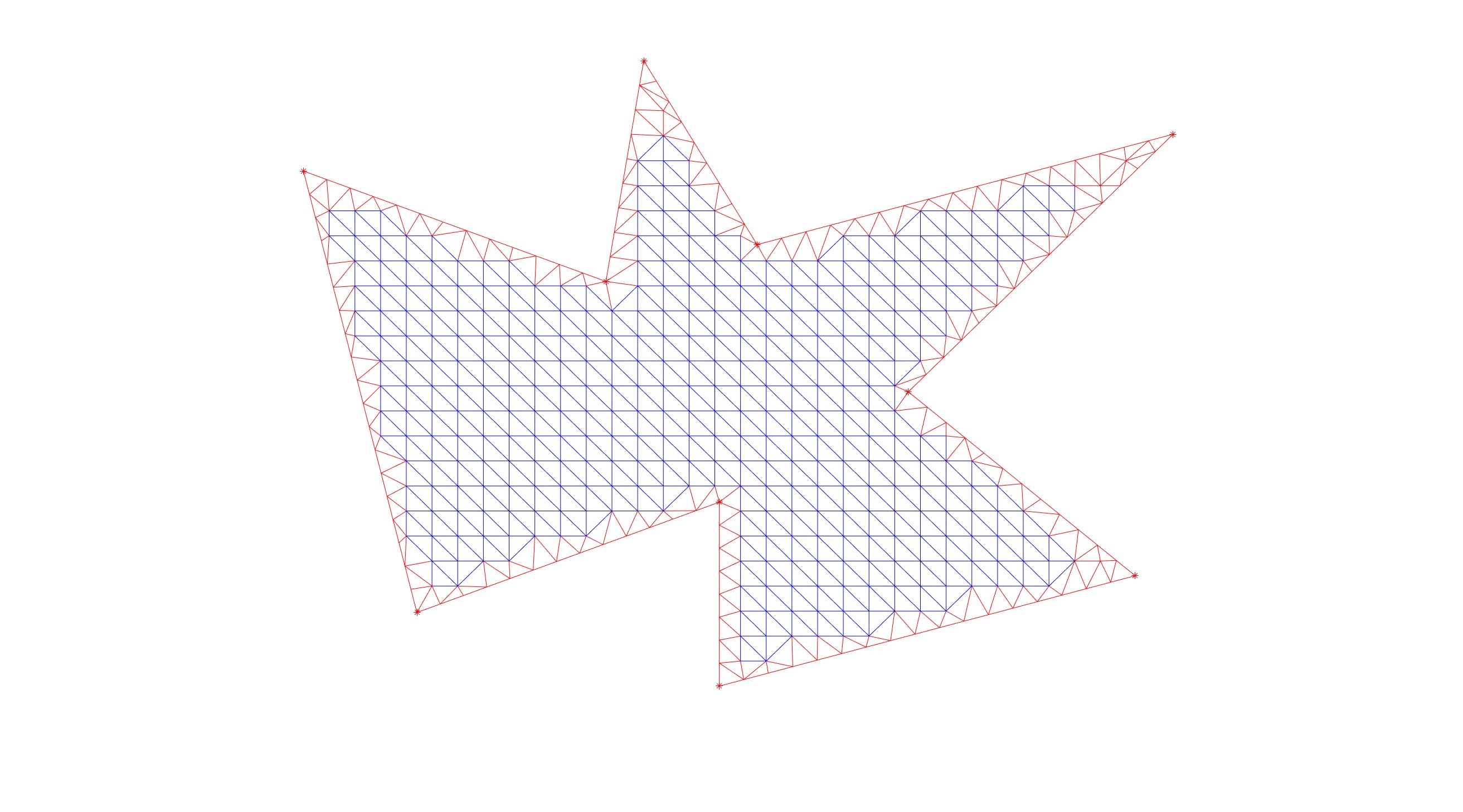
Figure 1. Illustration of $\triangle^{\circ}$ (in blue) inside a triangulation $\triangle$ (all triangles in red and blue)

It is known that there is no analytic representation of harmonic GBCs $\phi_{i}$ when $\Omega$ is not a parallelogram. One has to compute them numerically. A standard approach is to use finite element method or more generally, multivariate spline method (cf. [10]). Similarly, $\psi_{i}$ have no analytic representation to the best of the authors’ knowledge. Of course, one can solve the Poisson equation in (1.4) numerically to obtain an approximation of $\psi_{i}$. Indeed, let $\triangle_{k}$ be the $k$th uniform refinement of $\triangle$ for an integer $k\geq 1$ if $d=2$ or $\triangle_{k}$ be a refined simplicial partition of $\triangle$ if $d\geq 3$ with $|\triangle_{k}|<|\triangle|$, where $|\triangle|$ the largest diameter of simplexes in $\triangle$. Thus, $|\triangle|$ is called the size of $\triangle$. Let $S_{i}=S_{\phi_{i}}$ be a spline approximation of $\phi_{i}$ over triangulation $\triangle_{k}$ and similarly $R_{i}=S_{\psi_{i}}$ be a spline approximation of $\psi_{i}$ over $\triangle_{k}$.

One of the significances of these functions is that we can use $\phi_{i},i=1,\cdots,N$ and $\psi_{j},j=1,\cdots,M$ to approximate the solution of any Dirichlet boundary value problem of the Poisson equation:

(1.6) $$\begin{cases}-\Delta u&=f,\quad{\bf x}\in\Omega\cr\quad u&=g,\quad{\bf x}\in\partial\Omega,\end{cases}$$

for any given $f\in L^{2}(\Omega)$ and $g\in L^{2}(\partial\Omega)$. For simplicial partition $\triangle$ of $\Omega$, we are interested in the approximation of $S_{i}$ and $R_{i}$ when $|\triangle|$ is small. Indeed, the following is one of the main results in this paper:

Theorem 1.3.

Suppose that $f$ is a piecewise continuous function in $L^{2}(\Omega)$ and $g$ is a piecewise continuous function in $L^{2}(\partial\Omega)$. Let $\triangle$ be a simplicial partition of $\Omega$ such that $H_{f}(x,y):=\sum_{i=1}^{m}f({\bf v}_{i})h_{i}(x,y)$ is a linear spline approximation of $f$ over $\Omega$, e.g. $f(x,y)-H_{f}(x,y)=O(|\triangle|^{2})$ and $L_{g}:=\sum_{{\bf v}_{i}\in\partial\Omega}g({\bf v}_{i})S_{i}$ is a linear spline approximation of $g$ on $\partial\Omega$, i.e., $\|g-L_{g}\|_{L^{2}(\partial\Omega)}=O(|\triangle|^{2})$. Then the solution $u$ to (4.1) can be approximated by

(1.7) $$u\approx\sum_{{\bf v}_{i}\in\triangle^{\circ}}f({\bf v}_{i})\psi_{i}+\sum_{{\bf v}_{i}\in\partial\Omega}g({\bf v}_{i})\phi_{i}\approx\sum_{{\bf v}_{i}\in\triangle^{\circ}}f({\bf v}_{i})R_{i}+\sum_{{\bf v}_{i}\in\partial\Omega}g({\bf v}_{i})S_{i}.$$

That is, letting $L_{u}=L_{f}+L_{g}$ with $L_{f}=\sum_{{\bf v}_{i}\in\triangle^{\circ}}f({\bf v}_{i})R_{i}$ and $L_{g}=\sum_{{\bf v}_{i}\in\partial\Omega}g({\bf v}_{i})S_{i}$, we have

$$\|\nabla(u-L_{u})\|=O(|\triangle|).$$

Proof.

As expected, $L_{u}$ is just like the standard finite element solution. We shall give a proof in a later section. See §3 for a detailed proof and numerical experimental results which support the statement in (1.7). In addition, a comparison with the numerical results from the standard finite element method will be shown. ∎

Remark 1.4.

We remark that the GBC solution $L_{u}=L_{f}+L_{g}$ is not an FEM solution. For simplicity, let us say the solution $u$ satisfying the zero boundary condition. In this case, $L_{u}=L_{f}$ which is a linear combination of $f({\bf v}_{i}),{\bf v}_{i}\in{\triangle}^{\circ}$ while the FEM solution is a linear combination of the coefficient vector ${\bf c}$ which is the solution of the linear system $K{\bf c}=M{\bf f}$, where $K$ and $M$ are the stiffness and mass matrices, respectively.

Let us continue to discuss the locality of these harmonic GBC functions. First of all, we need to explain that a numerical harmonic GBC function $S_{i}$ approximates the exact harmonic GBC function $\phi_{i}$ very well. Similar for $R_{i}$ for $\psi_{i}$. Therefore, the e-locality of $\phi_{i}$ and $\psi_{i}$ can be seen from the e-locality of $S_{i}$ and $R_{i}$, respectively. To avoid a pathological example, we assume that the number of distinct boundary vertices is more than $4$ as most applied problems have a lot of boundary vertices.

For a simplicial partition $\triangle$ of $\Omega$, we say it is $\beta$-quasi-uniform if there is a positive number $\beta>0$ such that

(1.8) $$\max_{T\in\triangle}\frac{|{\triangle}|}{\rho_{T}}\leq\beta,$$

where $\rho_{T}$ is the radius of the inscribed ball of simplex $T$. Let $S^{r}_{n}(\triangle)$ be the spline space of degree $d$ and smoothness $r\geq 0$, e.g. when $n=1$ and $r=0$, $S^{0}_{1}(\triangle)$ is the standard continuous finite element space. In general, we can use any $n\geq 1$ and $r\geq 0$ as long as $n\geq 3r+2$ if $\Omega\subset\mathbb{R}^{2}$. Otherwise, we can use $n=1$ and $r=0$ or $n\geq 9$ and $r=1$. See [29] for trivariate splines. There are two numerical implementation methods of multivariate splines which can be found in [4] and [36] as well as other efficient implementations in [33] and [40]. Recall $\phi_{i}\in H^{1}(\Omega)$ be a GBC function in the Sobolev space $H^{1}(\Omega)$ satisfying (1.1) and $S_{i}$ is the minimizer of the following minimization (1.9) over the spline space $S^{r}_{n}(\triangle)$ of degree $n$ and smoothness $r\geq 0$:

(1.9) $$\begin{cases}\min_{u\in S^{r}_{n}(\triangle)}&\int_{\Omega}|\nabla u|^{2},\cr u&=\ell_{i},\quad{\bf x}\in\partial\Omega.\end{cases}$$

We split $S_{i}$ into $S_{i,0}$ and $G_{i}$. That is, $S_{i}=S_{i,0}+G_{i}\in S^{r}_{n}(\triangle)$, where $G_{i}\in S^{r}_{n}(\triangle)$ satisfies the boundary condition $G_{i}=\ell_{i}$ on $\partial\Omega$ and $S_{i,0}\in H^{1}_{0}(\Omega)\cap S^{r}_{n}(\triangle)$. Then $S_{i}$ satisfies the following weak formulation:

(1.10) $$\langle\nabla S_{i,0},\nabla\psi\rangle=-\langle\nabla G_{i},\nabla\psi\rangle,\quad\forall\psi\in S^{r}_{n}({\triangle})\cap H^{1}_{0}(\Omega).$$

It is easy to see that $S_{i}$ is a numerical harmonic GBC which approximates $\phi_{i}$ very well in the following sense:

(1.11) $$\|\nabla(S_{i}-\phi_{i})\|\leq C_{\phi_{i}}|\triangle|^{d}$$

by using the well-known Ceá lemma, where $C_{\phi_{i}}$ is a positive constant dependent on $\phi_{i}$, d, and $\Omega$. Furthermore, there is a maximum norm estimate, i.e.

(1.12) $$\|S_{i}-\phi_{i}\|_{\infty}\leq C_{\phi_{i}}log(|\triangle|)|\triangle|^{d+1}.$$

We refer to [9] for detail. Similarly, $R_{i}\in S^{r}_{n}(\triangle)$ is the weak solution satisfying

(1.13) $$\langle\nabla R_{i},\nabla\psi\rangle=-\langle h_{i},\psi\rangle,\quad\forall\psi\in S^{r}_{n}({\triangle})\cap H^{1}_{0}(\Omega).$$

The standard finite element theory shows that $R_{i}$ satisfies the same inequalities as $S_{i}$ in (1.11) and (1.12). Hence, one can see that the locality of $\psi_{i}$ can be estimated based on the locality of $R_{i}$. We leave the proof of (1.11) and (1.12) to Appendix.

In terms of spline functions, the exponential decay can be recast more precisely. Let $\hbox{star}^{1}({\bf v}_{i})$ be the union of all simplexes in $\triangle$ sharing vertex ${\bf v}_{i}$ and $\hbox{star}^{k}({\bf v}_{i})$ is the union of all simplexes in $\triangle$ sharing vertices in $\hbox{star}^{k-1}({\bf v}_{i})$ for $k\geq 2$. We will show that there exists a constant $\sigma\in(0,1)$ such that

(1.14) $$|S_{i}({\bf v})|\leq C\sigma^{k}\hbox{ and }|R_{i}({\bf v})|\leq C\sigma^{k},\hbox{ if }{\bf v}\not\in\hbox{star}^{k}({\bf v}_{i})$$

for a positive constant $C$ independent of $i$. That is, if ${\bf v}$ is a far away from ${\bf v}_{i}$ according to the triangulation $\triangle$ (cf. Definition 2.1), $|S_{i}({\bf v})|$ is close to zero. Similar for $R_{i}$. See the statement of Theorem 2.6 in the next section for more detail.

The rest of the paper is devoted to the estimate (1.14) of the e-locality of $S_{i}$ and $R_{i}$ by using a theoretical approach which was used in study of the domain decomposition methods for scattered data interpolation and fitting (cf. [30]) and the convergence of discrete least squares (cf. [18]). We shall present some numerical e-locality of our GBC functions. See §4. In addition, an application to numerical solution to Poisson equations using our GBC functions will be demonstrated in §5, where Theorem 1.3 will be proved.

2. The Exponential Decay Property of Boundary and Interior GBC Functions

Let us start with an explanation of some useful concepts, notations, and definitions on spline spaces. For each vertex ${\bf v}\in\triangle$, let $\hbox{star}({\bf v})$ be the collection of all simplexes from $\triangle$ attached to ${\bf v}$. Similarly, for each simplex $T\in\triangle$, let $\hbox{star}(T)$ be the collection of all simplexes in ${\triangle}$ connected to $T$. Next for each integer $\ell>1$, let $\hbox{star}^{\ell}({\bf v})$ the the collection of all simplexes in ${\triangle}$ which is connected to $\hbox{star}^{\ell-1}({\bf v})$ with $\hbox{star}^{1}({\bf v}):=\hbox{star}({\bf v})$ for $\ell>1$. Similar for $\hbox{star}^{\ell}(T)$. See an example in Figure 2 for $\hbox{star}^{\ell}(T)$ for $\ell=1,2,3$ in the setting of $\mathbb{R}^{2}$.

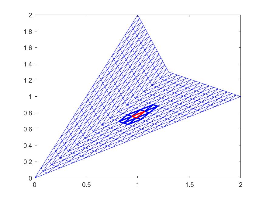
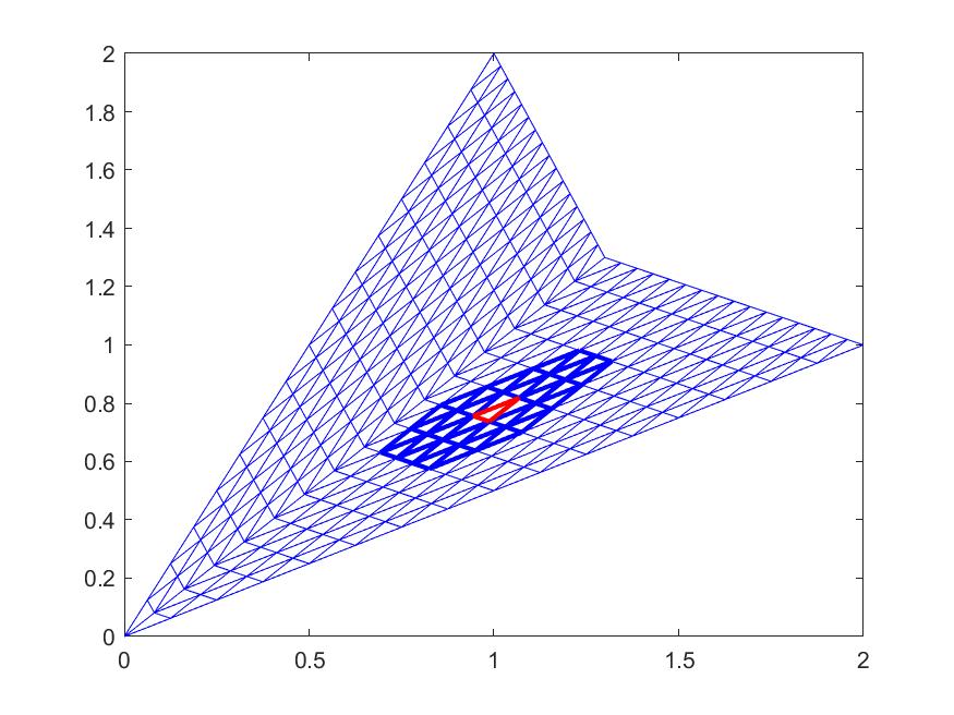
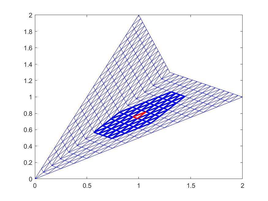
Figure 2. Illustration of $\hbox{star}^{1}(T),\hbox{star}^{2}(T),\hbox{star}^{3}(T)$ over a triangulation with $T$ shown in red

Now we define a measure between two points ${\bf x},{\bf y}\in\Omega$ based on triangulation $\triangle$ in the following sense:

Definition 2.1.

We say a point ${\bf x}\in\Omega$ is $k$-simplexes away from another point ${\bf y}\in T\in\triangle$ is ${\bf x}\not\in\hbox{star}^{k}(T)$, but in $\hbox{star}^{k+1}(T)$. We say ${\bf x}$ is far away from ${\bf y}\in T$ or from $T$ is ${\bf x}\not\in\hbox{star}^{k}(T)$ for positive integer $k\gg 1$.

Next let $B_{\xi},\xi\in\mathcal{M}$ be a basis for $S^{r}_{n}(\triangle)$, where $\mathcal{M}$ is an index set. For an integer $\ell\geq 1$, we say $B_{\xi},\xi\in\mathcal{M}$ is stable and $\ell$-local in the sense that there is a positive constant $K_{1}$ such that for all indices $\xi\in\mathcal{M}$,

(2.1) $$\|B_{\xi}\|_{\infty,\Omega}\leq K_{1},$$

and there is an integer $\ell\geq 1$ for all $\xi\in\mathcal{M}$,

(2.2) $$\hbox{supp}(B_{\xi})\subseteq\hbox{star}^{\ell}(T_{\xi}),$$

for a simplex $T_{\xi}\in{\triangle}$ associated with index $\xi$, where the constant $K_{1}$ may be dependent only on $\ell$ and the smallest angle in ${\triangle}$.

There are many spaces which have stable local bases. For example, in Euclidean space $\mathbb{R}^{d}$ with $d\geq 2$, the continuous spline spaces $S^{0}_{n}({\triangle})$ have stable local bases with $\ell=1$ for any degree $n\geq 1$. In $\mathbb{R}^{2}$ the same is true for the superspline spaces $\mathcal{S}^{r,2r}_{4r+1}({\triangle})$ for all $r\geq 1$ of degree $4r+1$ and smoothness $r$ and supersmoothness $2r$ at vertices. E.g. $S^{1,2}_{5}(\triangle)$, the Argyris $C^{1}$ quintic finite element space with super smoothness $C^{2}$ at vertices. In [29], several families of macro-element spaces defined for all $r\geq 1$ with the same property are explained. We refer to [18] for more such spaces.

We now use the format of multivariate Bernstein polynomials to write each polynomial over a simplex $T$ (see [8], [6], and [29] for detail). For polynomial $u\in\mathbb{P}_{n}$, we write

(2.3) $$u({\bf x})=\sum_{i_{0}+i_{1}+\cdots+i_{d}=n}c_{i_{0},\cdots,i_{d}}\frac{n!}{\prod_{j=0}^{d}i_{j}!}\prod_{j=0}^{d}b_{j}^{i_{j}},$$

where $b_{0},\cdots,b_{d}$ are barycentric coordinates of point ${\bf x}$ with respect to $T=\langle{\bf v}_{0},\cdots,{\bf v}_{d}\rangle$. Let ${\bf c}=(c_{i_{0},\cdots,i_{d}},i_{0}+\cdots+i_{d}=n)$ be the coefficient vector of $u$. Following the proof of Theorem  2.7 for the $\mathbb{R}^{2}$ setting and/or the proof of Theorem 15.9 (for the $\mathbb{R}^{3}$ setting) in [29], we can show

(2.4) $$\frac{V_{T}^{1/2}}{K}\|{\bf c}\|_{2}\leq\|u\|_{2,T}\leq V_{T}^{1/2}\|{\bf c}\|_{2},\quad\forall u\in\mathbb{P}_{n}$$

for a positive constant $K$ dependent only on $n$, where $V_{T}$ is the volume of simplex $T$. Letting

(2.5) $$\phi_{\xi}=\frac{n!}{\prod_{j=0}^{d}i_{j}!}\prod_{j=0}^{d}b_{j}^{i_{j}},$$

with $\xi=\{i_{0},\cdots,i_{d},T\}$, we note that there are redundancies for the collection $\{\phi_{\xi},\xi=(i_{0},\cdots,i_{d},T),T\in\triangle,i_{0}+\cdots+i_{d}=n\}$ due to the neighboring simplexes. Indeed, if two simplexes $T_{1}$ and $T_{2}$ sharing a common face, there is $\phi_{\xi}$ for some $\xi$ associated with $T_{1}$ and $\phi_{\eta}$ for $\eta$ associated with $T_{2}$ which are the same function on the common face $T_{1}\cap T_{2}$. For these two functions, we let $B_{\xi}$ be the function which is piecewise defined on the union $T_{1}\cup T_{2}$ with $B_{\xi}=\phi_{\xi}$ on $T_{1}$ and $B_{\xi}=\phi_{\eta}$ on $T_{1}$. Let us delete the index $\eta$ from the whole index set $\{\xi=(i_{0},\cdots,i_{d},T),T\in\triangle,i_{0}+\cdots+i_{d}=n\}$. For simplicity, let us show $B_{\xi}$ in the 2D setting in Figure 3.

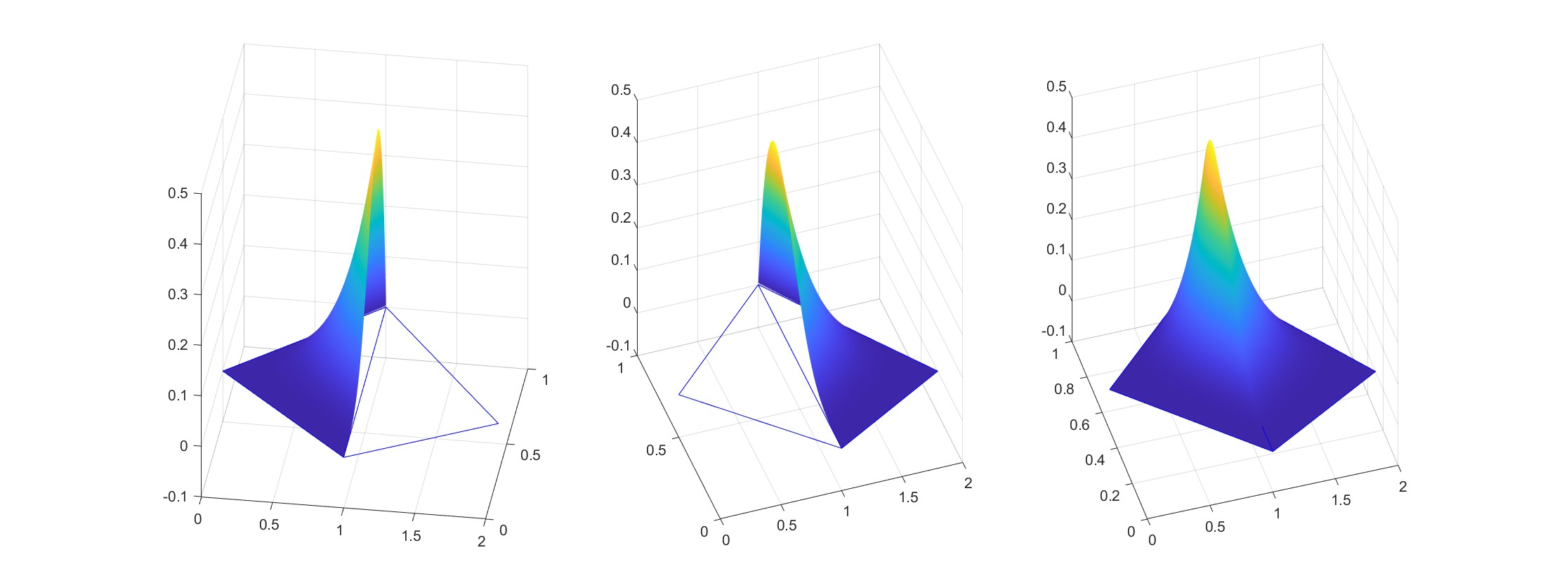
Figure 3. Construction of $B_{\xi}$ over $T_{1}\cup T_{2}$ shown on the right based on $\phi_{\xi}$ (left) and $\phi_{\eta}$(middel)

For another case, if a vertex ${\bf v}$ shared by more than one simplex, there will be more than one function $\phi_{\xi}$ with $\xi$ on $T_{1},\cdots,\eta$ on $T_{k}$ which have the common value at the vertex, we let $B_{\xi}$ be the spline function which is $\phi_{\xi}$ on $T_{1}$, $\cdots,$ $B_{\xi}=\phi_{\eta}$ on $T_{k}$ if $T_{1},\cdots,T_{k}$ share the vertex ${\bf v}$. We delete all the indices $\eta$ on $T_{2},\cdots,T_{k}$ from the whole index set. We do the same thing for other common facets such as edges, …, $(d-2)$ facets sharing by more than one simplex from $\triangle$. For the remaining indices $\xi$, we let $B_{\xi}=\phi_{\xi}$. Let us put these $B_{\xi}$ together to form $\{B_{\xi},\xi\in\mathcal{M}\}$ which is a basis for $S^{0}_{n}(\triangle)$, where $\mathcal{M}\subset\{\xi:T\in\triangle,i_{0}+\cdots+i_{d}=n\}$ is the subset after deleting the redundant indices mentioned above.

We are now ready to explain the exponential decay property of the GBC functions. Let us first begin with a key result, Lemma 2.3 whose proof can be found in [30]. The similar results hold in the multivariate setting which will be stated in Theorem 2.4. The proof of Theorem 2.4 relies on the following stability of spline functions.

Lemma 2.2.

Suppose that $S^{0}_{n}(\triangle)$ is a continuous spline space of degree $n$ defined on a $\beta$-quasi-uniform simplicial partition $\triangle$ of polyhedral domain $\Omega\subset\mathbb{R}^{d}$ with $d\geq 2$. Let $\mathcal{W}=H^{1}_{0}(\Omega)\cap S^{0}_{n}(\triangle)$ be a subspace with inner product $\langle f,g\rangle_{\mathcal{W}}=\langle\nabla f,\nabla g\rangle$ and norm $\|f\|_{\mathcal{W}}:=\|\nabla f\|$. Then there exist two positive constants $C_{1},C_{2}$, the following equalities

(2.6) $$C_{1}\sum_{\xi\in\mathcal{M}}|c_{\xi}|^{2}\leq\big{\|}\sum_{\xi\in\mathcal{M}}c_{\xi}\mathcal{B}_{\xi}\big{\|}_{\mathcal{W}}^{2}\leq C_{2}\sum_{\xi\in\mathcal{M}}|c_{\xi}|^{2}$$

hold for all coefficient vectors ${\bf c}:=\{c_{\xi}\}_{\xi\in\mathcal{M}}$, where $\{\mathcal{B}_{\xi}\}_{\xi\in\mathcal{M}}$ is an 1-local basis for $\mathcal{W}$.

Proof.

Let $\mathbb{P}_{n}$ be the space of polynomials of degree $\leq n$ in $\mathbb{R}^{d}$. Let $\mathbb{T}$ be the set of all simplexes $T$ with one vertex at ${\bf 0}$ and $1/\beta\leq\rho_{T}\leq|T|=1$, where $\rho_{T}$ is the radius of the ball inscribed in $T$ and $|T|$ is the diameter of the minimum ball containing $T$. Let

$$C_{1}:=\inf_{T=\langle{\bf v}_{1},\cdots,{\bf v}_{d+1}\rangle\in\mathbb{T}}\{\|\nabla p\|_{T}^{2}\hbox{ such that }p\in\mathbb{P}_{n},\int_{T}p^{2}=1,p({\bf v}_{1})=0\}.$$

Then there exist sequences $p_{k},T_{k}$ of polynomials and simplexes, respectively, such that $p_{k}\to p\in\mathbb{P}_{n}$ and $T_{k}\to T\in\mathbb{T}$ with $\int_{T}p^{2}=1$ and $C_{1}=\|\nabla p\|_{T}^{2}$. We claim that $C_{1}>0$. Indeed, if $\|\nabla p\|_{T}^{2}=0$, then $p\in\mathbb{P}_{0}$. But then using the fact that $p$ vanishes at one vertex, it follows that $p\equiv 0$, contradicting $\int_{T}p^{2}=1$. We have shown that $C_{1}>0$ and that it certainly depends only on $\beta$, $n$, and $d$.

Next let

$$C_{2}:=\sup_{T=\langle{\bf v}_{1},\cdots,{\bf v}_{d+1}\rangle\in\mathbb{T}}\{\|\nabla p\|_{T}^{2}\hbox{ such that }p\in\mathbb{P}_{n},\int_{T}p^{2}=1,\hbox{ and }p({\bf v}_{1})=0\}.$$

Clearly, by using the Markov inequality, it is easy to see that $C_{2}<\infty$. Certainly, $C_{2}$ depends only on $\beta$, $d$, and $n$. Now if $T$ is an arbitrary simplex in $\triangle$, then after translating one vertex to ${\bf 0}\in\mathbb{R}^{d}$ and substituting ${\bf x}=|T|\widetilde{{\bf x}}$, we see that for any $u\in\mathcal{W}$,

(2.7) $$C_{1}\int_{T}u^{2}\leq|T|^{d}\|\nabla u\|_{T}^{2}\leq C_{3}\int_{T}u^{2}.$$

Combining (2.7) and (2.4) together, we have

(2.8) $$\|\nabla u\|_{T}^{2}\leq C_{3}|T|^{-d}\int_{T}u^{2}\leq C_{3}|T|^{-d}V_{T}\|{\bf c}\|_{2}^{2}=C_{4}\|{\bf c}\|_{2}^{2}$$

for a positive constant $C_{4}$ and

(2.9) $$\|\nabla u\|_{T}^{2}\geq C_{1}|T|^{-d}\int_{T}u^{2}\geq C_{1}/K|T|^{-d}V_{T}\|{\bf c}\|_{2}^{2}=C_{0}\|{\bf c}\|_{2}^{2}$$

for another positive constant $C_{0}$. Then summing over all simplexes in $\triangle$ gives 2.6 with new constants $C_{1}$ and $C_{2}$ with a consideration of the redundant indices over the common facets of neighboring simplexes of $\triangle$. Indeed, it is easy to see that the largest number of redundant indices is the largest number of simplexes sharing a common vertex ${\bf v}\in\triangle$. Let ${\bf v}\in\triangle$ be the vertex sharing by $k_{\bf v}$ number of simplexes in $\triangle$. Let $N_{\bf v}$ be the ball centered at ${\bf v}$ with radius $|\triangle|/2$. It is easy to see all simplexes sharing ${\bf v}$ are inside $N_{\bf v}$. The volume of $N_{\bf v}$ is less or equal to $A\pi(|\triangle|/2)^{d}$ for a positive constant $A$. As each of these simplexes contains the inscribed ball with radius $\rho_{\triangle}$ which has a volume $A\pi(\rho_{\triangle})^{d}$. It follows that number $k_{\bf v}$ of simplexes in $\triangle$ sharing ${\bf v}$ is estimated by

$$k_{v}\leq\frac{A\pi(|\triangle|/2)^{d}}{A\pi\rho_{\triangle}^{d}}=\frac{1}{2^{d}}\beta^{d}<\infty.$$

That is, $C_{2}=C_{4}\frac{1}{2^{d}}\beta^{d}$ and $C_{1}=C_{0}$. ∎

With the estimates (2.6) in the bivariate setting, Lai and Schumaker in [30] proved the following result.

Lemma 2.3 (Lai and Schumaker, 2009 [30]).

Let $\omega$ be a cluster of triangles in ${\triangle}$, and let $T\in\omega$ be a triangle, e.g. $\omega=T$. Then there exists constants $0<\sigma<1$ and $C$ depending only on the ratio $C_{2}/C_{1}$ in (2.6) such that if $g$ is a function in $\mathcal{W}$ with

(2.10) $$\langle g,\,w\rangle_{\mathcal{W}}=0,\qquad\hbox{ for all }w\in\mathcal{W}\hbox{ with supp(}w)\subseteq\hbox{star}^{k}(\omega),$$

for some fixed $k\geq 1$, then

(2.11) $$\|g\cdot\chi_{T}\|_{\mathcal{W}}\leq C\sigma^{k}\|g\|_{\mathcal{W}},$$

where $\chi_{T}$ is the characteristic function of $T$.

Now let us translate the result in Lemma 2.3 in the setting of $\Omega\subset\mathbb{R}^{d},d\geq 2$ to have

Theorem 2.4.

Let $\triangle$ be a simplicial partition of $\Omega\subset\mathbb{R}^{d},d\geq 2$. Suppose that $\mathcal{W}$ has an $1$-stable basis $\{\mathcal{B}_{\xi}\}_{\xi\in\mathcal{M}}$ satisfying (2.6). Let $\omega$ be a cluster of simplexes in ${\triangle}$ or a simplex, e.g. $\omega=T$. Then there exists constants $0<\sigma<1$ and $C$ depending only on the ratio $C_{2}/C_{1}$ in (2.6) such that if $g$ is a function in $\mathcal{W}$ with

(2.12) $$\langle g,\,w\rangle_{\mathcal{W}}=0,\qquad\hbox{ for all }w\in\mathcal{W}\hbox{ with supp(w)}\subseteq\hbox{star}^{k}(\omega),$$

for some fixed $k\geq 1$, then

(2.13) $$\|g\cdot\chi_{T}\|_{\mathcal{W}}\leq C\sigma^{k}\|g\|_{\mathcal{W}},$$

where $\chi_{T}$ is the characteristic function of $T$.

Proof.

We use the ideas in the proof of Lemma 4.2 in [30] to establish this similar result in Theorem 2.4. The detail is omitted here. ∎

Note that the proof of Theorem 2.4 is based on the ideas in [19] and [18] and an elementary inequality in [5] which is included below.

Lemma 2.5 (de Boor, 1996[5]).

If the sequence $a_{0},a_{1},...$ satisfies

(2.14) $$|a_{m}|\geq c\sum_{j\geq m}|a_{j}|,\quad m=0,1,2,\cdots,$$

for some $c\in(0,1)$, then $\lambda=1-c\in(0,1)$ and

(2.15) $$|a_{m}|\leq|a_{0}|\lambda^{m}/c,\quad m=0,1,2,\cdots$$

This equality was called discrete Gronwall inequality as in [12]. Please notice that this exponential decay includes a linear decay as a special case. For example, let $k\geq 10$ be an integer and let

$$a_{0}=k,a_{1}=k-1,\cdots,a_{k}=0,a_{k+j}=0,\forall j\geq 1$$

be a sequence. Then it is clear that this sequence decays to zero in a linear fashion, but satisfies the de Boor condition (2.14) for $c=1/k$. Indeed, if $m\geq k$, we have (2.14) as the both sides are zero and if $0\leq m<k$, we have

$$c\sum_{j\geq m}|a_{j}|=\frac{1}{k}\sum_{i=1}^{k-m}i=\frac{k-m}{k}\frac{k-m+1}{2}\leq k-m=a_{m}.$$

Lemma 2.5 shows that this sequence is of exponential decay in the sense of (2.15). We shall use this sequence to explain the decay property of the GBC functions over a rectangular domain. That is, the GBC functions over a rectangular domain linearly decay to zero and satisfy the decay property (2.15).

We now explain how to use Theorem 2.4 for establishing the e-locality of our numerical harmonic GBC functions $S_{i}$ and $R_{i}$. First of all, we explain the e-locality of $S_{i}=S_{i,0}+G_{i}$. We start with $G_{i}$. Let us fix a simplicial partition $\triangle_{k}$ which is a refinement of $\triangle$ and fix a spline space, say $S^{1}_{n}(\triangle_{k})$ with $n\geq 5$ in $\mathbb{R}^{2}$ or $n\geq 9$ in $\mathbb{R}^{3}$ and etc. Then we can construct $G_{i}\in S^{1}_{n}(\triangle)$ satisfying the boundary condition, i.e. $G_{i}|_{\partial\Omega}=\ell_{i}$ as follows. Without loss of generality, we may assume that $\Omega$ is a star-shaped polygon in $\mathbb{R}^{2}$. There is a center ${\bf v}_{c}$ which can be connected to all vertices of $\Omega$. Let us form an initial triangulation in this way, say $\triangle_{0}$. Then our $\triangle_{k}$ is a uniformly refined triangulation of $\triangle_{0}$. Let us say $\triangle$ is the third refinement of $\triangle_{0}$.

If we use a continuous spline space $S^{0}_{n}(\triangle_{k})$ with $n\geq 1$, we can easily construct $G_{i}$ at boundary vertex ${\bf v}_{i}$. Indeed, let us use Figure 4 to show spline coefficients of $G_{i}$ in $S^{1}_{5}(\triangle_{0})$ over the domain points on three triangles. The remaining spline coefficients of $G_{i}$ over other triangles of $\triangle_{0}$ are all zero.

Figure 4. A Construction of $G_{1}$ over the two triangles sharing ${\bf v}_{1}$ using continuous spline space $S^{0}_{5}(\triangle)$

Next let us explain how to construct $G_{i}\in S^{1}_{5}(\triangle_{0})$. Once we have $G_{i}$, we can rewrite $G_{i}$ over $S^{1}_{5}(\triangle_{k})$ due to the nestedness of our spline spaces. On $S^{1}_{5}(\triangle_{0})$, $G_{1}$ can be constructed by specifying the coefficients as shown in Figure 5 over domain points of degree $5$ over $\triangle_{0}$. Note that ${\bf v}_{1},{\bf v}_{2},\cdots,{\bf v}_{N}$ are boundary vertices. ${\bf v}_{c}$ is an interior vertex. $u,v,X,Y\geq 0$ are coefficients which are dependent on $C^{1}$ smoothness conditions. That is, we use $C^{1}$ smoothness condition connected to the coefficients $1$, two $4/5$ and $Y$ to find $Y$ first if the edge ${\bf e}_{1}=\langle{\bf v}_{1},{\bf v}_{2}\rangle$ and the edge $\langle{\bf v}_{1},{\bf v}_{N}\rangle$ are not parallel. Then we find two positive values $X$ by solving the $C^{1}$ smoothness condition connecting the coefficients $Y$, $0$ and $X,X$. If the edge ${\bf e}_{1}=\langle{\bf v}_{1},{\bf v}_{2}\rangle$ and the edge $\langle{\bf v}_{1},{\bf v}_{N}\rangle$ are parallel, we simply choose $Y=0$ and hence, $X=0$. Next we use the $C^{1}$ smoothness condition to find $u$ and then $v$. The remaining coefficients of $G_{1}$ are all zero which we do not show in Figure 5. Hence, this function $G_{1}$ is in $S^{1}_{5}(\triangle_{0})$.

Figure 5. A Construction of $G_{1}\in S^{1}_{5}(\triangle_{0})$ over three triangles sharing ${\bf v}_{1}$

In the same way, we can construct $G_{i}\in S^{0}_{n}(\triangle_{k})$ or in $S^{1}_{n}(\triangle_{k})$ for $\triangle_{k}$ in the higher dimensional setting. We leave the detail to the interested reader. It is clear that $G_{i}$ is of exponential decay. To show the e-locality of $S_{i}$, we only need to discuss the e-locality of $S_{i,0}$ with $S_{i,0}=S_{i}-G_{i}$.

To this end, let $\Omega_{i}=\hbox{star}^{1}({\bf v}_{i})$ be the union of all simplexes which are connected to the boundary vertex ${\bf v}_{i}$. According to the construction above, the support of $G_{i}$ is contained in $\Omega_{i}$ in both $C^{0}$ and $C^{1}$ cases. We say a simplex $T$ is L-simplex away from the boundary $\partial\Omega$ if $L$ is the smallest integer such that there exist $L$ simplexes $T_{1},\cdots,T_{L+1}$ in $\triangle$ such that $T=T_{1}$ and $\bar{T}_{L+1}\cap\partial\Omega\not=\emptyset$ as well as $\bar{T}_{j}\cap\bar{T}_{j+1}\not=\emptyset$ for $j=1,\cdots,L$. Furthermore, we say $T$ is $L$-simplex away from the boundary $\partial\Omega$ in the opposite direction of ${\bf v}_{i}$ if there exists an integer $k$ such that $\hbox{star}^{k}(T)\subset\Omega_{i}^{c}$, the complement of $\Omega_{i}$ in $\Omega$ and $T_{i}\in\hbox{star}^{k+\ell_{i}}(T)\subset\Omega_{i}^{c}$ for $\ell_{i+1}\geq\ell_{i}\geq 0$ for $i=1,\cdots,L+1$. See Figure 6 for ${\bf v}_{i}$ (the red dot), $\Omega_{i}$, $T=T_{1}$, $T_{2}$ and $T_{4}$, where $T_{3}$ can be any triangle between $T_{2}$ and $T_{4}$ as long as $T_{3}\cap T_{2}\not=\emptyset$ and $T_{3}\cap T_{4}\not=\emptyset$. There are three choices for $T_{3}$.

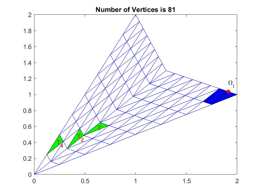
Figure 6. Illustration of $T$ whose $\hbox{star}^{5}(T)\subset\Omega_{i}^{c}$ and $T_{2}$ and $T_{4}$. Note that $T_{3}$ is not shown. It can be any triangle between $T_{2}$ and $T_{4}$ as long as $T_{3}\cap T_{2}\not=\emptyset$ and $T_{3}\cap T_{4}\not=\emptyset$.

We are now ready to state and prove one of the main results in this paper.

Theorem 2.6.

Fix a boundary vertex ${\bf v}_{i}\in\Omega$. Suppose that $\Omega_{i}=\hbox{star}({\bf v}_{i})\not=\Omega$. Let ${\bf v}\in\Omega$ be a point in $\Omega\setminus\Omega_{i}$. Let $T\in\triangle$ contain ${\bf v}$, i.e. ${\bf v}\in T$. Suppose $k\geq 1$ is the integer such that $\hbox{star}^{k}(T)\subset\Omega_{i}^{c}$, the complement of $\Omega_{i}$ in $\Omega$ and $L\geq 1$ is another integer such that $T$ is $L$ simplexes away from the partial boundary $\partial\Omega\backslash\Omega_{i}$ in the opposite direction of ${\bf v}_{i}$. Then there exists a positive constant $K>0$ independent of $L$ and $\sigma\in(0,1)$ such that

(2.16) $$|S_{i}({\bf v})|\leq K(L+1)\sigma^{k}.$$

Proof.

It is easy to see from the construction of $G_{i}$ above that $G_{i}$ is only supported over $\Omega_{i}$. Since $\Omega_{i}\subset\Omega$ and $\Omega_{i}\not=\Omega$, $G_{i}$ has e-locality. That is, $G_{i}$ decays to zero outside of $\Omega_{i}$. We only need to show that $S_{i,0}=S_{i}-G_{i}$ has e-locality. According the assumptions, $\hbox{star}^{k}(T)\cap\Omega_{i}=\emptyset$. By (1.10), we use $S_{i,0}$ for $g$ in Theorem 2.4 and use (1.10) to have

$$\langle g,\,w\rangle_{\mathcal{W}}:=\langle\nabla S_{i,0},\nabla w\rangle=-\langle\nabla G_{i},\nabla w\rangle=0,$$

for all $w\in\mathcal{W}$ with $\hbox{sup}(w)\subseteq\hbox{star}^{k}(T)$. Therefore, we can use the result from Theorem 2.4 above to conclude that there exists a positive number $\sigma\in(0,1)$ such that

(2.17) $$\|\nabla S_{i,0}\cdot\chi_{T}\|\leq C\sigma^{k}\|\nabla S_{i,0}\|.$$

We now show $\|S_{i,0}\|_{\infty}$ can be bounded by the left-hand side of (2.17). To do so, let us use induction on $L\geq 1$. If $L=1$, then $T$ is one simplex away from the partial boundary $\partial\Omega\backslash\Omega_{i}$ in the opposite direction of ${\bf v}_{i}$. Let ${\bf v}\in T\cap T_{2}$ and ${\bf u}\in T_{2}\cap(\partial\Omega\backslash\Omega_{i})$. That is, ${\bf u}$ on the partial boundary and hence $S_{i,0}({\bf u})=0$. By Taylor expansion with remainder, we have

$$0=S_{i,0}({\bf u})=S_{i,0}({\bf v})+\nabla S_{i,0}({\bf w})({\bf u}-{\bf v})$$

for a point ${\bf w}\in T$ in the line segment between ${\bf u}$ and ${\bf v}$. It follows that

$$|S_{i,0}({\bf v})|=|\nabla S_{i,0}({\bf w})({\bf u}-{\bf v})|\leq|\triangle|\|\nabla S_{i,0}\|_{\infty,T_{2}}\leq C\|\nabla S_{i,0}\|_{L^{2}(T_{2})}=C\|\nabla S_{i,0}\cdot\chi_{T_{2}}\|$$

by Theorem 1.1 of [29] over triangle $T_{2}$. Similarly, we have the same estimate for polynomials over simplex $T$ in $\mathbb{R}^{d}$ if $d>2$. We now use (2.17) to conclude

$$|S_{i,0}({\bf v})|\leq C\sigma^{k}\|\nabla S_{i,0}\|.$$

As $\|\nabla S_{i,0}\|=\|\nabla(S_{i}-G_{i})\|$ is very close to $\|\nabla(\phi_{i}-G_{i})\|$ by (1.11), there exists a constant $K>0$ dependent on $\nabla\phi_{i}$ such that

$$|S_{i,0}({\bf v})|\leq C\sigma^{k}\|\nabla S_{i,0}\|\leq C\sigma^{k}\|\nabla(S_{i}-\phi_{i})\|+C\sigma^{k}\|\nabla(\phi_{i}-G_{i})\|\leq K\sigma^{k}.$$

Hence, $|S_{i}({\bf v})|=\|S_{i,0}({\bf v})|\leq K\sigma^{k}.$

Next assume that when $T$ is $(L-1)$-simplex away from the partial boundary of $\Omega$ in the opposite direction of ${\bf v}_{i}$, we have the desired estimate. Let us consider the case when $T$ is $L$-simplex away from the partial boundary of $\Omega$ in the opposite direction of ${\bf v}_{i}$. Let ${\bf u}_{L}\in T_{L}$ be the intersection of $T_{L}$ and $T_{L+1}$ and $T_{L+1}$ intersects the partial boundary. By the argument above, we have

$$|S_{i,0}({\bf u}_{L})|\leq K\sigma^{k+\ell_{L}}.$$

for an integer $\ell_{L}$ with $\ell_{L}\geq 0$. For ${\bf u}_{j}\in T_{j}\cap T_{j+1}$ with $j=1,\cdots,L-1$ with ${\bf u}_{1}={\bf v}$, we use Taylor expansion again to have

$$S_{i,0}({\bf u}_{j})=S_{i,0}({\bf u}_{j+1})+\nabla S_{i,0}({\bf w})({\bf u}_{j}-{\bf u}_{j+1})$$

for an appropriate ${\bf w}\in T_{j}$. It follows that

$$|S_{i,0}({\bf u}_{j})|\leq|S_{i,0}({\bf u}_{j+1})|+|{\triangle}|\|S_{i,0}\|_{\infty,T_{j}}\leq|S_{i,0}({\bf u}_{j+1})|+C\|\nabla S_{i,0}\|_{L^{2}(T_{j})}$$

by Theorem 1.1 of [29] again and

$$|S_{i,0}({\bf v})|\leq\cdots\leq K\sigma^{k+\ell_{L}}+\sum_{j=1}^{L}C\|\nabla S_{i,0}\|_{L^{2}(T_{j})}.$$

As $T_{j}$ is in the opposite direction of ${\bf v}_{i}$, similar to (2.17), we have $\|\nabla S_{i,0}\|_{L^{2}(T_{j})}\leq C\sigma^{k+\ell_{j}}\|\nabla S_{i,0}\|$. We put these inequalities together to have the desired result follows. We have thus completed the proof. ∎

When $S_{i}$ is a GBC function over a rectangular domain $\Omega$, the above arguments show that $S_{i}$ satisfies the decay problem (2.16) although $S_{i}$ decays linearly. We can say that $S_{i}$ decays in the sense of (2.15). Except for this pathological example, the GBC functions have indeed e-locality as shown in Example 2.7, i.e. Figures 8 and 9 and numerical experiments the researchers and practitioners have already observed.

Example 2.7.

Consider a quadrilateral and a triangulation $\triangle$ shown on Figure 7

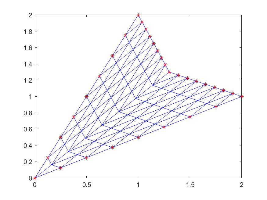
Figure 7. A triangulation of polygon $\Omega$ with boundary vertices

We use $S^{1}_{5}(\triangle)$ to approximate harmonic GBC functions. There are 32 GBC functions associated with boundary vertices shown in red in Figure 7. For convenience, we show 6 of them to illustrate that these functions clearly have e-decay property.

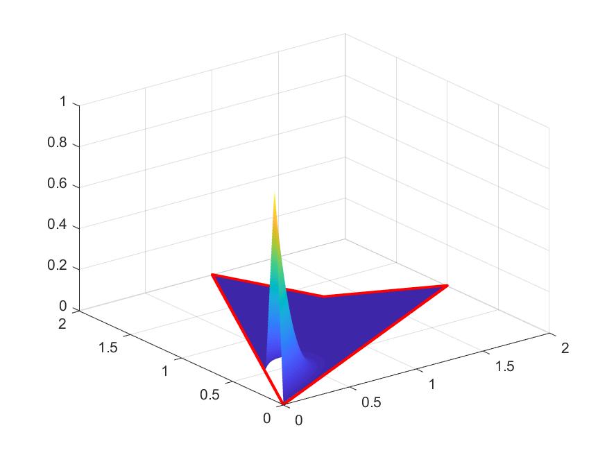
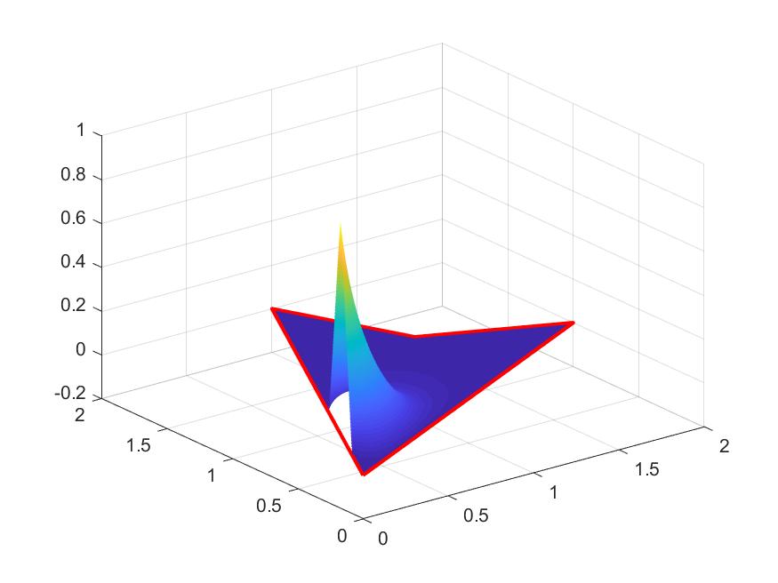
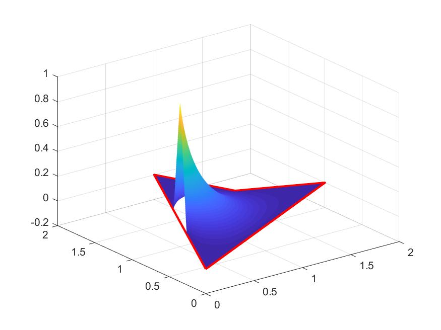
Figure 8. Spline Approximation of Various Harmonic GBC Functions on the Boundary of a Polygon.

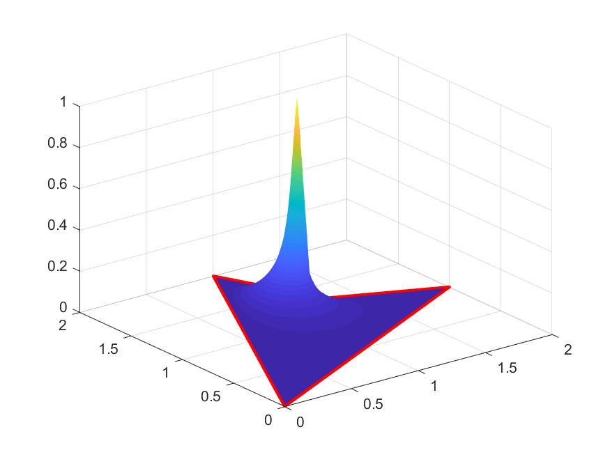
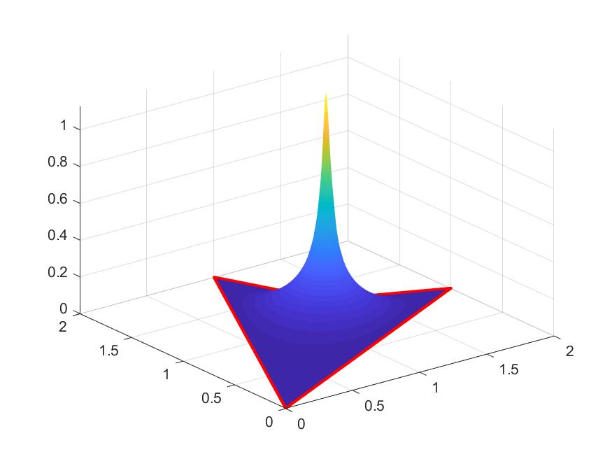
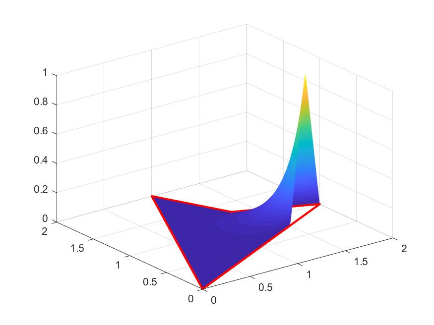
Figure 9. Spline Approximation of Various Harmonic GBC Functions on the Boundary of a Polygon

From graphs above, we clearly see the e-decay property of various spline harmonic GBC functions. Similar for other 26 GBC functions $S_{i}$ which are not shown here.

Next we show the e-locality of spline harmonic function $R_{i}$. Let $\omega_{i}$ be the support of function $h_{i}$ and $\widetilde{\Omega}_{i}$ be the union of all $\hbox{star}^{1}(t),t\in\omega_{i}$. Similar to $S_{i}$, we have

Theorem 2.8.

Let ${\bf v}\in\Omega$ be a point in $\Omega$ which is not in $\widetilde{\Omega}_{i}$. Let $T\in\triangle$ contain ${\bf v}$, i.e. ${\bf v}\in T$. Suppose that $k\geq 1$ is an integer such that $\hbox{star}^{k}(T)\subset\widetilde{\Omega}_{i}^{c}$, the complement of $\widetilde{\Omega}_{i}$ in $\Omega$. Suppose that $T$ is $L$ simplexes away from the boundary $\partial\Omega$ opposite to ${\bf v}_{i}$. Then there exists a positive constant $K>0$ independent of $L$ and $\sigma\in(0,1)$ such that

(2.18) $$|R_{i}({\bf v})|\leq K(L+1)\sigma^{k}.$$

Proof.

For any triangle $T\in\Omega\backslash\widetilde{\Omega}_{i}$, we know $\hbox{star}^{k}(T)\cap\widetilde{\Omega}=\emptyset$. By (6.1), we use $R_{i}$ for $g$ in Theorem 2.4 and (2.12) to have

$$\langle g,\,w\rangle_{\mathcal{W}}:=\langle\nabla R_{i},\nabla w\rangle=\langle h_{i},w\rangle=0,$$

for all $w\in\mathcal{W}$ with $\hbox{sup}(w)\subseteq\hbox{star}^{k}(T)$. Therefore, it follows from Theorem 2.4 that there exists a positive number $\sigma\in(0,1)$ such that

(2.19) $$\|\nabla R_{i}\cdot\chi_{T}\|\leq C\sigma^{k}\|\nabla R_{i}\|.$$

Next we use induction on $L\geq 1$. The argument is the same as the proof of Theorem 2.6. We omit the detail here to complete the proof. ∎

Example 2.9.

Consider a quadrilateral and a triangulation $\triangle$ shown on Figure 7. We use $S^{1}_{5}(\triangle)$ to approximate interior-harmonic GBC functions. There are 49 GBC functions associated with interior vertices shown in Figure 7. For convenience, we show 6 of them in Figure 10 and 11, where these functions also have e-decay property.

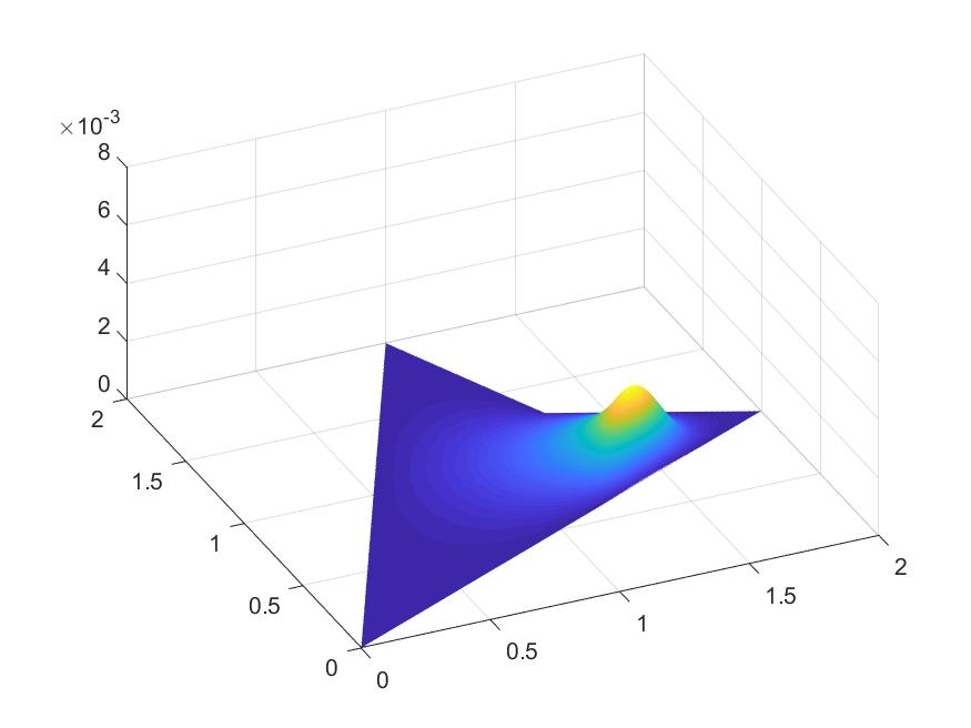
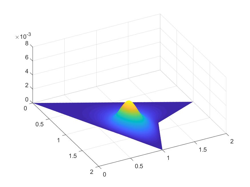
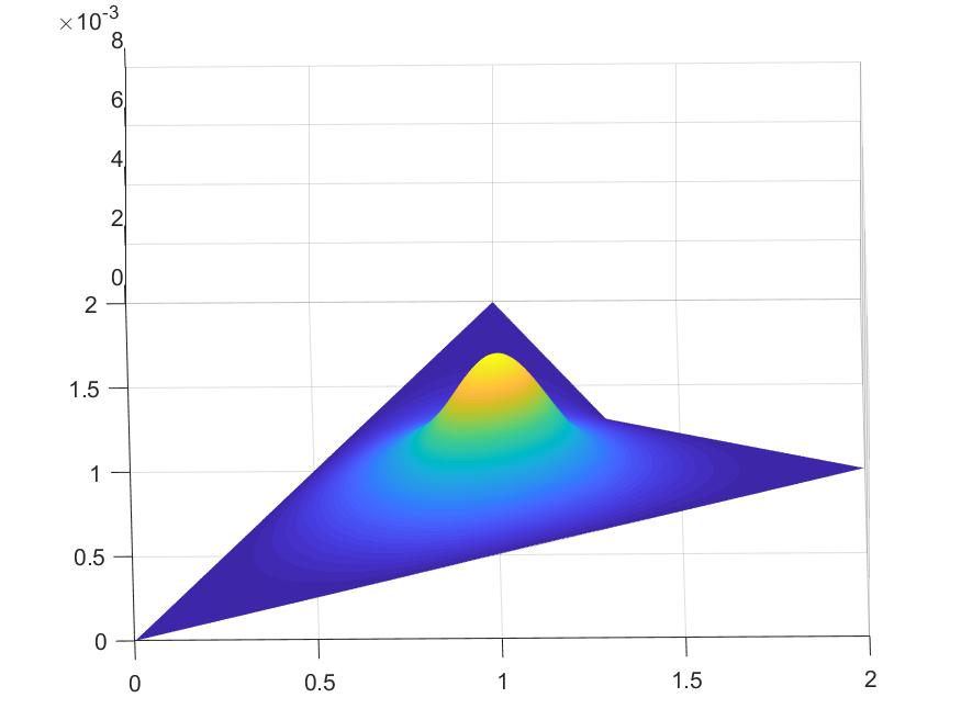
Figure 10. Spline Approximation of Various Interior-Harmonic GBC Functions over the Polygon

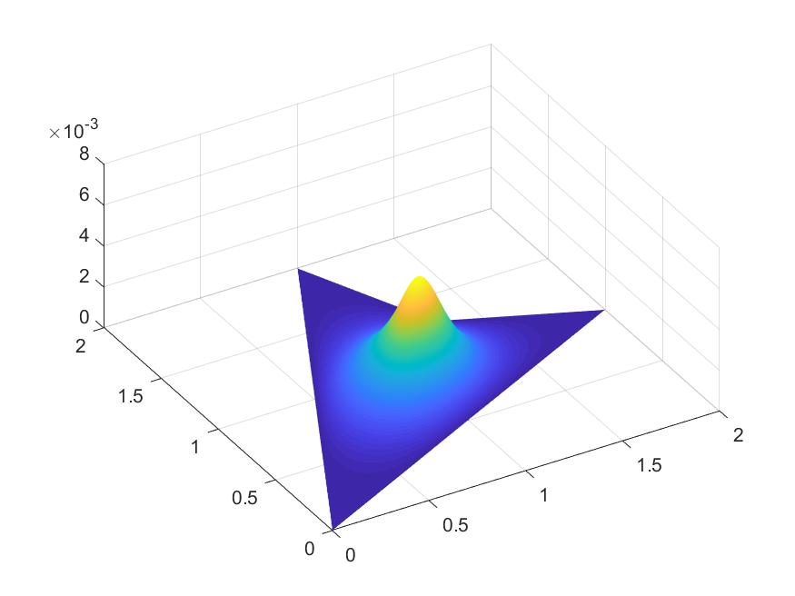
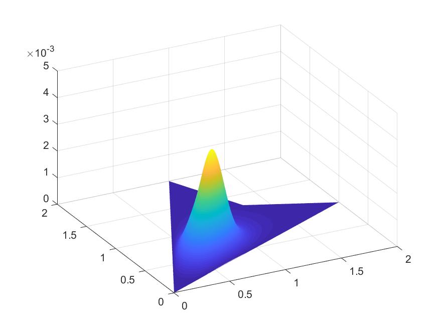
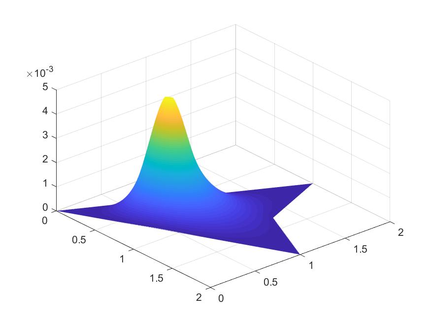
Figure 11. Spline Approximation of Various Interior-Harmonic GBC Functions

From graphs above, we clearly see the e-decay property of various spline interior harmonic GBC functions. Similar for remaining 43 GBC functions $R_{i}$ which are not shown here.

3. Local Boundary and Interior GBC Functions

In this section, we explore the e-locality of GBC functions using a numerical method. Mainly, it is interesting to know how small $\sigma\in(0,1)$ is. As the $\sigma$ is small, it makes sense to use GBC functions supported over star${}^{k}({\bf v})$ to approximate the GBC function with supporting vertex ${\bf v}$ for some fixed $k\geq 1$. For convenience we simply use a convex polygon(as shown on the left in Figure 12) to numerically compute a spline approximation of GBC functions (boundary and interior) globally and locally, respectively based on the computational triangulation (the right as shown in Figure 12). That is, for each boundary vertex (the red points given in Figure 12), we compute the standard GBC functions. For each interior vertex (the vertices inside the polygon on the left graph), we compute the interior GBC function. Here we say k-local GBC functions if the GBC function with supporting vertex ${\bf v}$ is computed based on the star${}^{k}({\bf v})$ for each $k\geq 1$. In general, we should use $k\geq 2$.

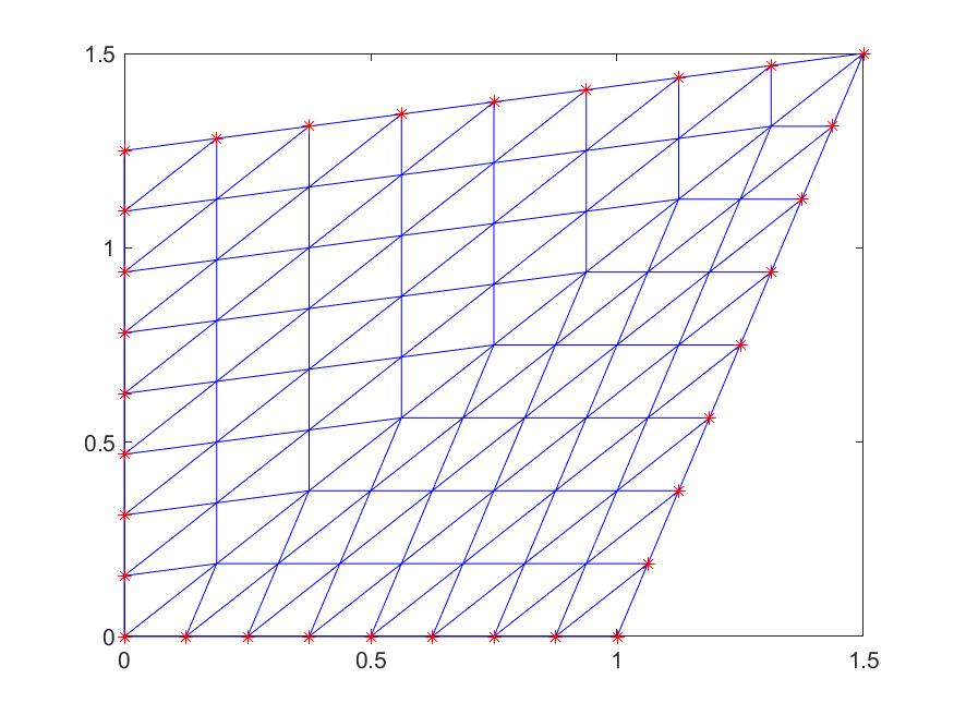
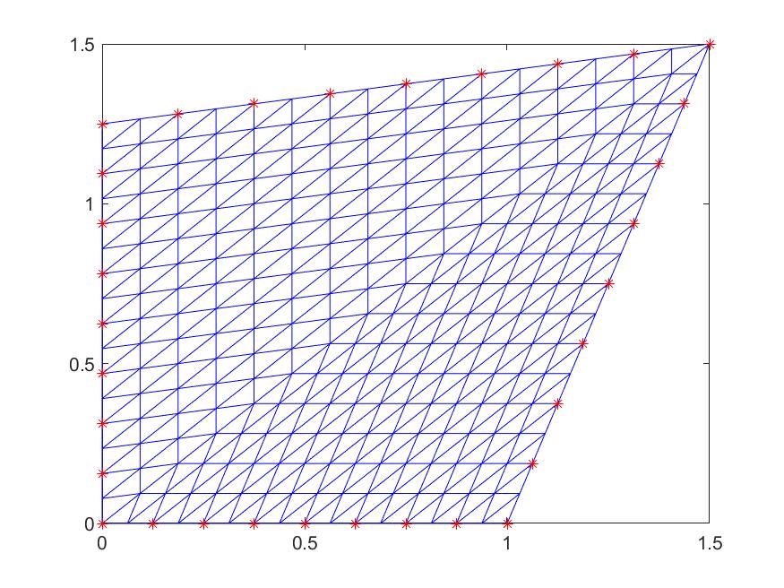
Figure 12. A triangulation of polygon $\Omega$ with boundary vertices and its refinement

Fix a boundary vertex ${\bf v}_{i}$ with $i\in V_{B}$. Let $t_{i}$ be a triangle in $\triangle$ with ${\bf v}_{i}$ as one of its vertex. For each ring number $k\geq 1$, let $V_{k},T_{k}$ be the triangulation of star${}^{k}(t_{i})$ shown in Figure 13.

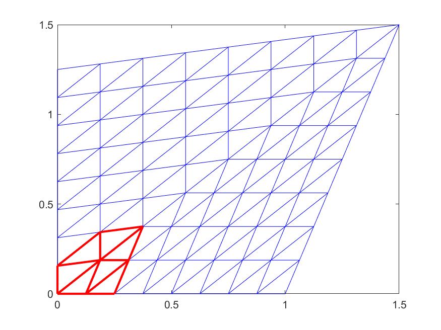
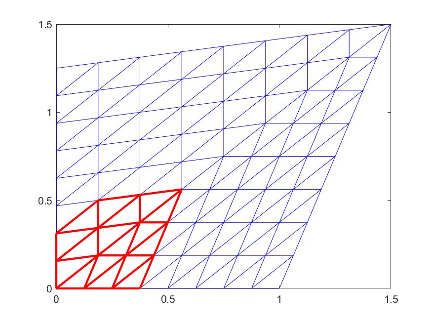
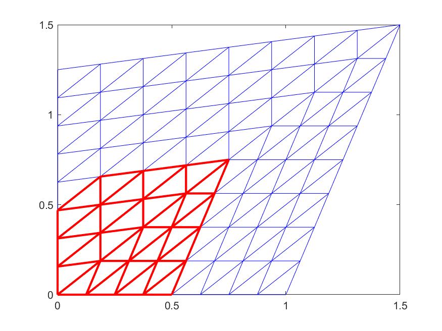
Figure 13. Various star${}^{k}(t_{0})$ for $k=1,2,3$

Let us first show how to compute a boundary GBC locally. Fix $k\geq 1$. Let us compute $S_{k}(\phi_{i})$ over the triangulation $\triangle_{k}=\cup_{t\in T_{k}}t$ at the boundary vertex ${\bf v}_{i}$. Then we compare the accuracies of the local GBC functions against the global GBC function supporting at ${\bf v}_{i}$. In Figure 14, we show the (global) GBC function and its local versions, where $t_{0}:={\bf v}_{i}$.

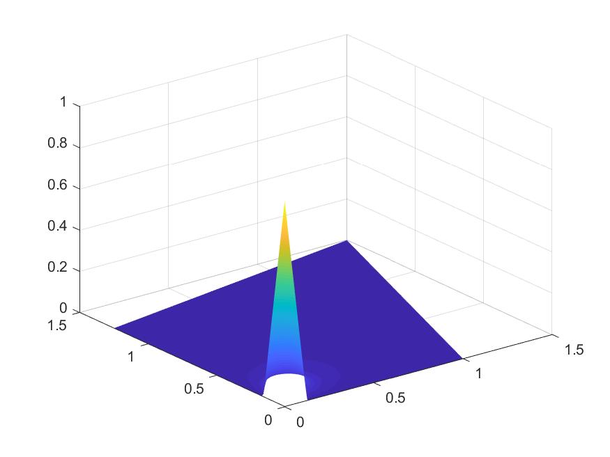
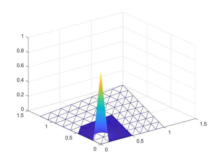
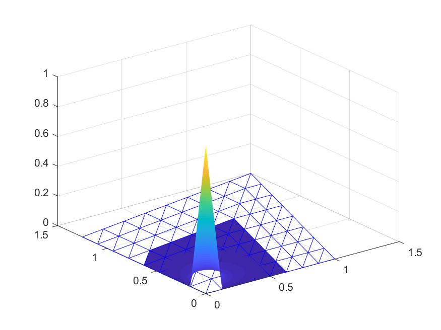
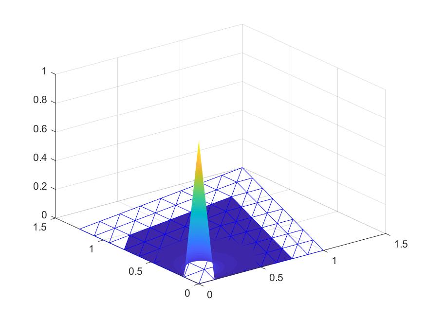
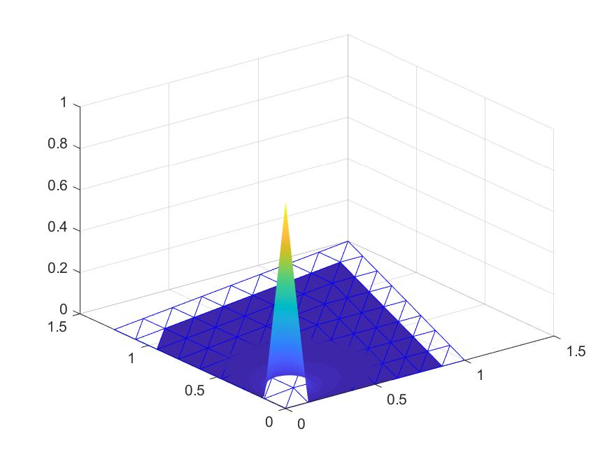
Figure 14. A GBC function and its local versions over star${}^{k}(t_{0})$ for $k=2,3,\cdots,6$.

Based on those 10,201 equally-spaced points of the bounding box of the polygon which fall into the polygon, we compute the maximum errors of these local GBC approximations shown in Figures 14 against the global GBC. These maximum errors are presented in Table 1.

Table 1. Local Approximations of $S_{i}$

no. of rings	max errors	rates
2	0.0132
3	0.0072	0.5455
4	0.0042	0.5833
5	0.0024	0.5714
6	0.0011	0.4583

From the ratios in Table 1, we can see that the rate of decay is about $0.5$. These numerical results show that we can use local GBCs to replace the (global boundary) GBCs for various applications of GBC functions such as polygonal domain deformation. This will result a great saving of computational time when a polygonal domain is complicated such as the domain of a giraffe or a crocodile. Indeed, due to the sensitivity of human eye, an error of $0.0011$ over a graph/image will not be detected by a normal humanbeing.

Similarly, we can compute local GBC approximations for each interior GBC function $R_{i}=S_{\psi_{i}}$. For each interior vertex ${\bf v}_{i}$, we let star${}^{k}({\bf v}_{i})$ be the k-th disk of triangles sharing the vertex ${\bf v}_{i}$.

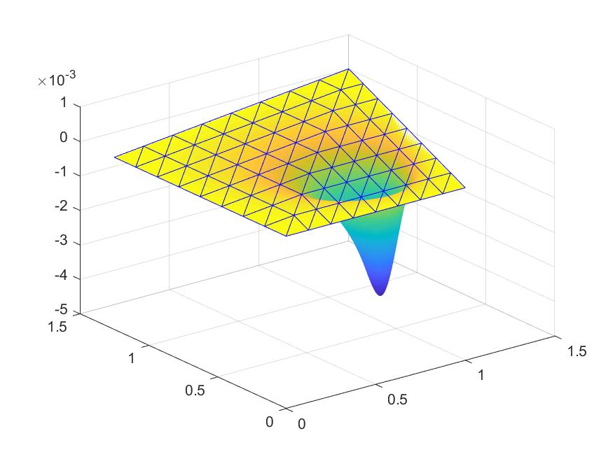
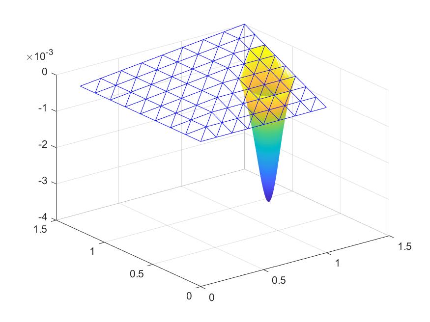
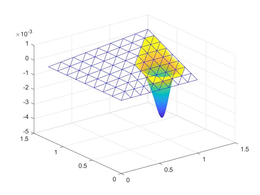
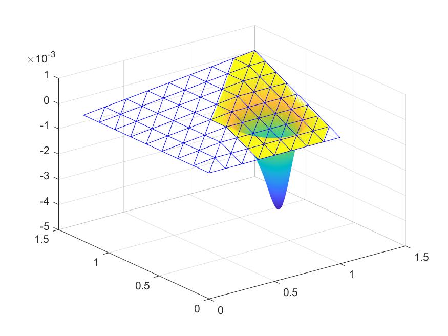
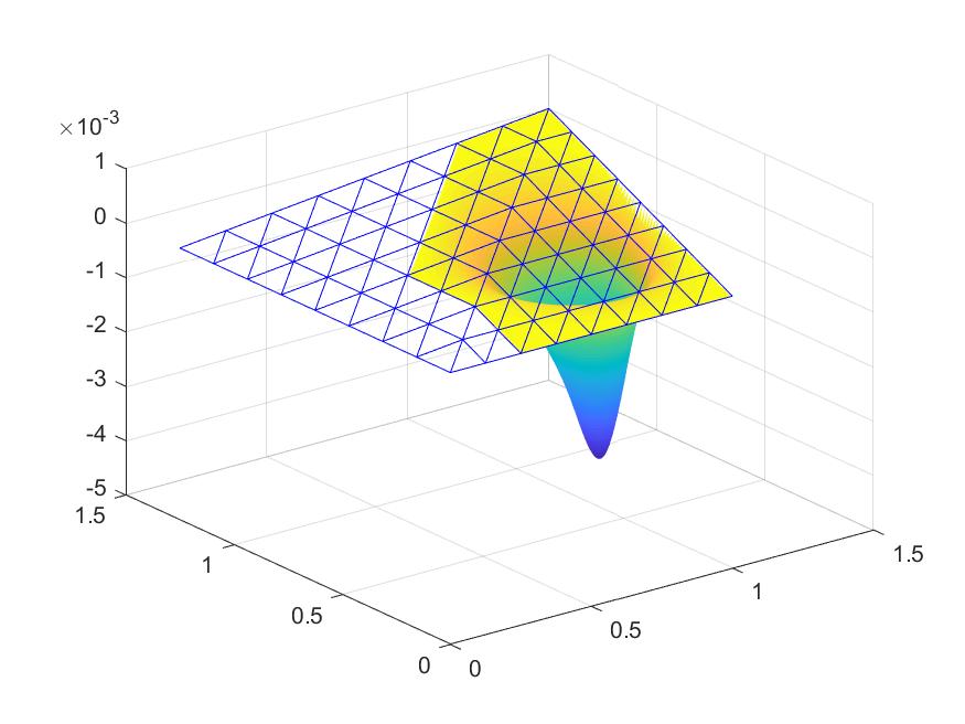
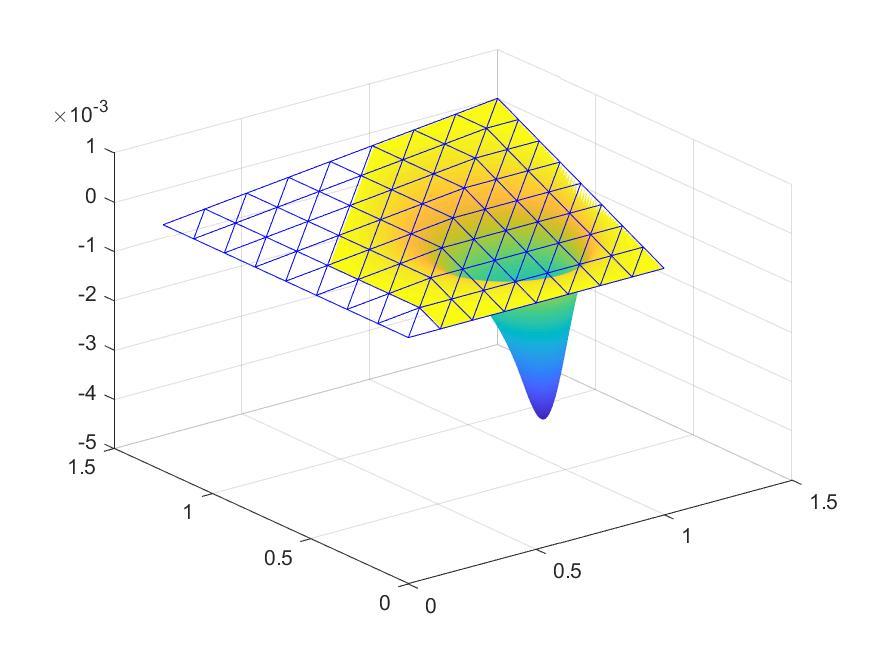
Figure 15. An interior GBC function and its local versions over star${}^{k}({\bf v}_{i})$ for $k=4$, $k=5$, and $k=6$.

The maximum errors of these local GBC approximations shown in Figures 14 against the global GBC are given in Table 2. Again, we compute the errors based on those 10,201 equally-spaced points of the bounding box of the polygon which fall into the polygon. From the Table 2, we can see that the averaged decay rate is about $0.68$.

Table 2. Local Approximations of $R_{i}$

no. of rings	max errors	rates
2	0.002500
3	0.001800	0.72
4	0.001200	0.66
5	0.000843	0.70
6	0.000559	0.66

Due to the e-locality of these harmonic GBC functions, we can use $k$-local GBC functions to approximate the globally GBC functions for an integer $k=2,3,4,\ldots$.

4. Numerical Approximation of the Poisson Equation

We now use these boundary-GBC and interior GBC functions to approximate the solution to the Poisson equation. In this section, we use a simple domain to demonstrate that these GBC functions can indeed be used for numerical solution of PDE. Besides the domain in the previous section, we also use the convex domain as shown in Fig 12.

We shall test our method for Poisson equations with various right-hand sides:

(4.1) $$\begin{cases}-\Delta u&=f,\quad{\bf x}\in\Omega\cr u&=g,\quad{\bf x}\in\partial\Omega,\end{cases}$$

where $f$ and $g$ are computed based on testing functions

• case 1 $u=1/(1+x^{2}+y^{2})$,

• case 2 $u=x^{2}+3y^{3}+4xy$,

• case 3 $u=x^{4}+y^{4}$,

• case 4 $u=\sin(x)\exp(y)$ and

• case 5 $u=10\exp(-x^{2}-y^{2})$.

Our method is to use a continuous piecewise linear spline based on the triangulation shown in Figures 7 and 12 to approximate $f$ and piecewise linear spline on $\partial\Omega$ to approximate $g$. Then the GBC approximation of the solution $u$ is given by

(4.2) $$u_{gbc}=\sum_{i\in V_{B}}g({\bf v}_{i})\phi_{i}+\sum_{j\in V_{I}}f({\bf v}_{j})\psi_{j},$$

where $V_{B}$ and $V_{I}$ are the index set of the boundary vertices and the index set of interior vertices of the triangulation shown in Figure 7 or Figure 12, respectively. We use bivariate spline functions in $S^{1}_{5}(\triangle)$ to approximate $\phi_{i}$ and $\psi_{j}$. To have a good approximation, we refine the triangulation shown in Figure 7 and Figure 12 once and then compute spline approximation of these two types of GBC functions. That is, we have

(4.3) $$L_{u}=\sum_{i\in V_{B}}g({\bf v}_{i})S_{\phi_{i}}+\sum_{j\in V_{I}}f({\bf v}_{j})S_{\psi_{j}},$$

We now show that $L_{u}$ is a good approximation of $u$. That is, we are now ready to present a proof of Theorem 1.3.

Proof of Theorem 1.3.

First of all, let $s_{u}$ be the finite element approximation of $u$ over the simplicial partition $\triangle$. It is well-known that $\|\nabla(u-s_{u})\|=O(|\triangle|)$ (cf. [9]). Note that $s_{u}|_{\partial\Omega}=L_{u}|_{\partial\Omega}$. It follows that

$$\|\nabla(u-L_{u})\|^{2}=\langle\nabla(u-L_{u}),\nabla(u-s_{u})\rangle+\langle\nabla(u-L_{u}),\nabla(s_{u}-L_{u})\rangle.$$

We first use Cauchy-Schwarz inequality to the first term on the right to have

$$|\langle\nabla(u-L_{u}),\nabla(u-s_{u})\rangle|\leq\|\nabla(u-L_{u})\|\|\nabla(u-s_{u})\|=O(|\triangle|)\|\nabla(u-L_{u})\|.$$

Then we use the Green identity to the second term on the right to have

$$\langle\nabla(u-L_{u}),\nabla(s_{u}-L_{u})\rangle=-\langle\Delta(u-L_{u}),s_{u}-L_{u}\rangle=\langle f-H_{f},s_{u}-u\rangle+\langle f-H_{f},u-L_{u}\rangle$$

since $\Delta L_{g}=0$. Note that $H_{f}$ is a continuous piecewise linear approximation of $f$. Since $H_{f}$ is a good approximation of $f$, $\|f-H_{f}\|=O(|\triangle|^{2})$ by the given assumption, we have

$$|\langle f-H_{f},s_{u}-u\rangle|\leq\|f-H_{f}\|\|s_{u}-u\|=O(|\triangle|^{3})$$

and

$$|\langle f-H_{f},u-L_{u}\rangle|\leq\|f-H_{f}\|(\|u\|+\|L_{u}\|)\leq C(|\triangle|^{2})$$

as $\|L_{u}\|\leq\|L_{f}\|+\|L_{g}\|=\|f\|_{L^{2}(\Omega)}+\|g\|_{L^{\infty}(\partial\Omega)}+O(|\triangle|^{2})$, where we have used the GBC property of $S_{\phi_{i}}$’s and the constant $C$ is dependent on $\|u\|_{L^{2}(\Omega)}$, $\|f\|_{L^{2}(\Omega)}$, and $\|g\|_{L^{\infty}(\partial\Omega)}$.

Combining the above estimates, we have

$$\|\nabla(u-L_{u})\|^{2}\leq O(|\triangle|)\|\nabla(u-L_{u})\|+O(|\triangle|^{3})+C(|\triangle|^{2}).$$

In other words, when $|\triangle|$ small enough, we have

$$(\|\nabla(u-L_{u})\|-O(|\triangle|))^{2}\leq O(|\triangle|^{2})+O(|\triangle|^{3})+C(|\triangle|^{2})$$

or $\|\nabla(u-L_{u})\|\leq O(|\triangle|)$. These complete the proof. ∎

Remark 4.1.

When the domain $\Omega$ is of uniformly positive reach (cf. [17] and [28]), we know the solution $u$ of the Poisson equation is in $H^{2}(\Omega)$ when $u|_{\partial\Omega}=0$ and hence,

(4.4) $$\|\Delta(u-L_{u})\|_{L^{2}(\Omega)}=\|f-\Delta L_{f}\|_{L^{2}(\Omega)}=\|f-\sum_{{\bf v}_{i}\in\triangle^{\circ}}f({\bf v}_{i})h_{i}\|_{L^{2}(\Omega)}=O(|\triangle|).$$

Following the argument in [28], there is a positive constant $C>0$ such that

(4.5) $$\|u-L_{u}\|_{H^{2}(\Omega)}\leq C\|\Delta(u-L_{u})\|_{L^{2}(\Omega)},$$

where $\|\cdot\|_{H^{2}(\Omega)}$ is the standard $H^{2}$ norm in $H^{2}(\Omega)$.

Next we report our numerical results on the approximation of $L_{u}$ to $u$. We use cases 1 through 5 to denote these testing functions mentioned above. To see how well our method can approximate the exact solution, we present the maximum errors of the GBC solution against the exact solution. In addition,we compare our numerical results with the numerical results from the standard finite element method (i.e. continuous linear finite element method). For simplicity, we compare the maximum error of the numerical solutions from both method against the exact solution, where the maximum errors are computed based on $1,000\times 1,000$ equally spaced points of the bounding box of the domain $\Omega$ which are located inside and on the $\Omega$. See Tables 3 and 4.

Table 3. Numerical Approximation of $L_{u}$ over a Nonconvex Quadrilateral

	GBCmethod	FEM
case 1	0.0179	0.0171
case 2	0.3644	0.3827
case 3	0.3812	0.3506
case 4	0.0610	0.0610
case 5	0.1898	0.1824

Table 4. Numerical Approximation of $L_{u}$ over a Convex Quadrilateral

	GBCmethod	FEM
case 1	0.0188	0.0158
case 2	0.2444	0.5015
case 3	0.1911	0.2063
case 4	0.0175	0.0285
case 5	0.2076	0.1726

In addition, we refine the triangulation used to generate the numerical approximation in Table 4 twice and compute the maximum errors again. The results are given in Table 5. Note that two methods yield similar numerical results. For cases 2 and 4, our GBC method is more accurate.

Table 5. Numerical Approximation of $L_{u}$ over a Triangulation (the first row of each case) and its Refinement (the second row of each case)

	GBCmethod	FEM
case 1	0.00566	0.00439
	0.00155	0.00111
case 2	0.06955	0.14491
	0.01956	0.03888
case 3	0.05576	0.05542
	0.01524	0.01433
case 4	0.00451	0.00737
	0.00112	0.00185
case 5	0.05966	0.04446
	0.01596	0.01109

From these tables, we can see that the maximum errors of GBC approximation $L_{u}$ are similar to the finite element solutions. These verify Theorem 1.3 numerically. Thus, $L_{u}$ can indeed be used to approximate the solution of the Poisson equation. If the coefficients of these $S_{\phi_{i}}$ and $S_{\psi_{j}}$ can be precomputed and stored, then the computational time for numerical solution of the Poisson equation for any right-hand side and boundary condition will be greatly reduced. This gives a flexibility of solving the Poisson equation, e.g. it allows a modification of a few places in the boundary condition and/or a few places in the right-hand side to obtain updates of the solution straightforwardly instead of repeatedly solving the system of linear equations again. Furthermore, if each GBC function $S_{\phi_{i}}$ or $S_{\psi_{j}}$ is approximated by using its k-local versions for small $k$, say $k\leq 6$ and all of them are computed individually using a GPU simultaneously, the computational time for numerical solution of the Poisson equation will be even reduced if the computational domain for each $k$-local GBC function is smaller than a quarter of the entire domain in the 2D setting.

5. Conclusions

In this paper, we define a new type of GBC functions which are called interior-GBC functions based on harmonic equations. Also, we have demonstrated the e-locality of these GBC functions. That is, we showed that each GBC function decays to zero away from its supporting vertex as explained in Theorem 2.6 and Theorem 2.8. The proofs are based on a nice result from [30] and [18] on the decay of locally supported spline functions. Furthermore, we showed that the solution to the Poisson equation can be approximated by using the both GBC functions. One can even use the k-local version of these GBC functions to approximate the solution to Dirichlet problem of the Poisson equation. With a help of GPU processes, one can solve the Poisson equation more efficiently in the sense that we use a computer with a lot of GPUs to solve the Poisson equation for all $S_{i},R_{i}$. Once these solutions are done, for any right-hand side $f$ and boundary condition $g$, we simply use the linear combination

$$\sum_{i=1}^{m}f({\bf v}_{i})R_{i}+\sum_{i=1}^{N}g({\bf v}_{i})S_{i}$$

to have a numerical solution without solving any system of linear equations any more.

6. Appendix

In this Appendix, we mainly justify the approximation of $S_{i}=S_{\phi_{i}}$ of GBC function $\phi_{i}$ with supporting vertex ${\bf v}_{i}$ for $i\in V_{B}$. From (1.1), we know that $\phi_{i}$ satisfies the following weak formulation:

(6.1) $$\langle\nabla\phi_{i,0},\nabla\psi\rangle=-\langle\nabla G_{i},\nabla\psi\rangle,\quad\forall\psi\in H^{1}_{0}(\Omega),$$

where $\phi_{i,0}=\phi_{i}-G_{i}$. Together with (1.10), we have

(6.2) $$\langle\nabla(\phi_{i,0}-S_{i,0}),\nabla\psi\rangle=0,\forall\psi\in S^{r}_{n}(\triangle)\cap H^{1}_{0}(\Omega).$$

Let $B_{\phi_{i}}\in S^{r}_{n}(\triangle)$ be the best approximation of $\phi_{i}$ in the spline space $S^{r}_{n}(\triangle)$ satisfying the boundary condition $B_{\phi_{i}}=G_{i}$ on $\partial\Omega$. It follows that

(6.3) $$\|\nabla(\phi_{i}-S_{\phi_{i}})\|^{2} = \langle\nabla(\phi_{i}-S_{\phi_{i}}),\nabla(\phi_{i}-S_{\phi_{i}})\rangle$$

(6.4) $$= \langle\nabla(\phi_{i,0}-S_{i,0}),\nabla(\phi_{i}-B_{\phi_{i}})\rangle$$

(6.5) $$\leq \|\nabla(\phi_{i}-S_{\phi_{i}})\|\|\nabla(\phi_{i}-B_{\phi_{i}})\|$$

by using (6.2). That is,

$$\|\nabla(\phi_{i}-S_{\phi_{i}})\|\leq\|\nabla(\phi_{i}-B_{\phi_{i}})\|.$$

The computation of the quasi-interpolatory formula in [29] shows that we have $\|\nabla(\phi_{i}-B_{\phi_{i}})\|\leq C_{\phi_{i}}|\triangle|^{d}$. Therefore, we have (1.11). Hence, we have (1.12).

References

- [1] D. Anisimov, Barycentric coordinates and their properties, in Generalized Barycentric coordinates in Computer Graphics and Computational Mechanics, edited by K. Hormann and N. Sukumar, CRC Press, 2018.
- [2] D. Anisimov, C. Deng, and K. Hormann, Subdividing barycentric coordinates, Computer Aided Geometric Design, 43: 172-185, 2016.
- [3] D. Anisimov, D. Panozzo, and K. Hormann, Blended barycentric coordinates, Computer Aided Geometric Design, 52–53: 205-216, 2017.
- [4] G. Awanou, M. -J. Lai, and P. Wenston, The multivariate spline method for scattered data fitting and numerical solution of partial differential equations, In Wavelets and splines: Athens 2005, pages 24–74. Nashboro Press, Brentwood, TN, 2006.
- [5] C. de Boor, A Bound on the -Norm of -Approximation by Splines in Terms of a Global Mesh Ratio, 30(1976), 765–771.
- [6] C. de Boor, B-form basics, in: G. Farin, editor, Geometric modeling: Algorithms and new trends, SIAM Publication, Philadelphia, 1987, pp. 131–148.
- [7] J. Cao, Y. Xiao, Z. Chen, W. Wang and C. Bajaj, Functional Data Approximation on Bounded Domains using Polygonal Finite Elements, Computer Aided Geometric Design, 63:149 C163, 2018.
- [8] C. K. Chui and M. -J. Lai, Multivariate Vertex Splines and Finite Elements, Journal of Approximation Theory, vol. 60 (1990) pp. 245–343.
- [9] P. G. Ciarlet, The finite element method for elliptic problems, North Holland, Amsterdam, 1978.
- [10] C. Deng, X. Fan, M. -J. Lai, A Minimization Approach for Constructing Generalized Barycentric Coordinates and Its Computation, Journal of Scientific Computing, vol. 84, 11(2020).
- [11] C. Deng, Q. Chang, K. Hormann, Iterative coordinates, Computer Aided Geometric Design, 2020, 79, Article 101861.
- [12] J. Douglas, JR., T. Dupont and L. Wahlbin, Optimal error estimates for Galerkin approximations to solutions of two-point boundary value problems, Math. Comp., v. 29,1975, pp. 475–483.
- [13] M. Floater, Generalized barycentric coordinates and applications, Acta Numerica, 24 (2015), 161–214.
- [14] M. Floater, Mean value coordinates, Computer Aided Geometric Design 20(1), 19–27 (2003).
- [15] M. Floater, K. Hormann, and G. Kos, A general construction of barycentric coordinates over convex polygons, Advances in Computational Mathematics 24, 311–331 (2006).
- [16] M. Floater and M. -J. Lai, Polygonal spline spaces and the numerical solution of the Poisson equation, SIAM Journal on Numerical Analysis, (2016) pp. 797–824.
- [17] F. Gao and M. -J. Lai, A new regularity condition of the solution to Dirichlet problem of the Poisson equation and its applications, Acta Mathematica Sinica, vol. 36 (2020) pp. 21–39.
- [18] M. von Golitschek and L. L. Schumaker, Bounds on projections onto bivariate polynomial spline spaces with stable bases, Constr. Approx., 18 (2002), pp. 241–254.
- [19] M. von Golitschek, Lai, M. -J. and Schumaker, L. L., Bounds for Minimal Energy Bivariate Polynomial Splines, Numerisch Mathematik, vol. 93 (2002) pp. 315–331.
- [20] K. Hormann and M. Floater, Mean value coordinates for arbitrary planar polygons, ACM Transactions on Graphics 25(4), 1424–1441 (2006).
- [21] K. Hormann and N. Sukumar, Generalized Barycentric Coordinates in Computer Graphics and Computational Mechanics, Taylor & Francis, CRC Press, Boca Raton, 2017.
- [22] K. Hormann and N. Sukumar, Maximum entropy coordinates for arbitrary polytopes, in Symposium on Geometry Processing 2008, Eurographics Association, pp. 1513–1520.
- [23] A. Jacobson, I. Baran, J. Popovic, and O. Sorkine, Bounded biharmonic weights for real-time deformation, ACM Trans. Graph. 30 (4): 78 (2011).
- [24] P. Joshi, M. Meyer, T. DeRose, B. Green, and T. Sanocki, Harmonic Coordinates for Character Articulation, Pixar Technical Memo#06–02b, Pixar Animation Studio, 2006.
- [25] T. Ju, S. Schaefer, and J. Warren, Mean value coordinates for closed triangular meshes, ACM Transactions on Graphics, 24(3): 561-566, 2005.
- [26] J. Kosinka and M. Barton, Convergence of Wachspress coordinates: from polygons to curved domains, Advances in Computational Mathematics, 41(3), 489–505 (2015).
- [27] M. -J., Lai, and Lanterman, J., A polygonal spline method for general 2nd order elliptic equations and its applications, in Approximation Theory XV: San Antonio, 2016, Springer Verlag, (2017) edited by G. Fasshauer and L. L. Schumaker, pp. 119–154.
- [28] Lai, M. -J. and J. Lee, A multivariate spline based collocation method for numerical solution of partial differential equations, SIAM J. Numerical Analysis, to appear, 2022.
- [29] M. -J. Lai and L. L. Schumaker, Spline Functions over Triangulations, Cambridge University Press, 2007.
- [30] M. -J. Lai and L. L. Schumaker, A Decomposition Method for Computing Bivariate Splines, SIAM J. Numerical Analysis, 47 (2009), 911–928.
- [31] Jay Lanterman, Construction of Smooth Vertex Splines over Quadrilaterials, Ph.D. Dissertation, the University of Georgia, 2018.
- [32] G. Manzini, A. Russo, N. Sukumar, New perspectives on polygonal and polyhedral finite element methods, Math. Models Methods Appl. Sci., 24(8): 1665–1699, 2014.
- [33] C. Mersmann, Numerical Solution of Helmholtz equation and Maxwell equations, Ph.D. Dissertation, 2019, University of Georgia, Athens, GA.
- [34] A. Rand, A. Gillette, C. Bajaj, Quadratic serendipity finite elements on polygons using generalized barycentric coordinates, Math. of computation, 83(290): 2691–2716, 2014.
- [35] L. L. Schumaker, Spline Functions, Academic Press, 1978.
- [36] L. L. Schumaker, Spline Functions: Computational Methods, SIAM Publication, 2015.
- [37] L. L. Schumaker, Solving Elliptic PDE’s on Domains with Curved Boundaries with an Immersed Penalized Boundary Method, J. Scientific Computing, online on May 24, 2019.
- [38] N. Sukumar, Construction of polygonal interpolants: a maximum entropy approach, Int. J. Numer. Meth. Engng 61, (2004) 2159–2181.
- [39] N. Sukumar and A. Tabarraei, Conforming polygonal finite elements, Int. J. Numer. Meth. Engng 61, (2004) 2045–2066.
- [40] Y. D. Xu, Multivariate Splines for Scattered Data Fitting. Eigenvalue Problems, and Numerical Solution to Poisson equations, Ph.D. Dissertation, 2019, University of Georgia, Athens, GA.
- [41] E. L. Wachspress, A Rational Finite Element Basis, Math. Sci. Eng. 114, Academic, New York, 1975.
- [42] Zhihao Wang, Yajuan Li, Weiyin Ma, Chongyang Deng, Positive and smooth Gordon-Wixom coordinates, Computer Aided Geometric Design, 2019, 74, Article 101774.
- [43] O. Web, R. Poranne, and G. Gotsman, Biharmonic coordinates, Computer Graphics Forum, 31(2012), pp. 2409–2422.
- [44] J. Zhang, B. Deng, Z. Liu, G. Patané, S. Bouaziz, J. Hormann, and L. Liu, Local Barycentric Coordinates, SIGGRAPH, Asia, 2014.