Tensor-based Multi-view Spectral Clustering via Shared Latent Space

Abstract

Multi-view Spectral Clustering (MvSC) attracts increasing attention due to diverse data sources. However, most existing works are prohibited in out-of-sample predictions and overlook model interpretability and exploration of clustering results. In this paper, a new method for MvSC is proposed via a shared latent space from the Restricted Kernel Machine framework. Through the lens of conjugate feature duality, we cast the weighted kernel principal component analysis problem for MvSC and develop a modified weighted conjugate feature duality to formulate dual variables. In our method, the dual variables, playing the role of hidden features, are shared by all views to construct a common latent space, coupling the views by learning projections from view-specific spaces. Such single latent space promotes well-separated clusters and provides straightforward data exploration, facilitating visualization and interpretation. Our method requires only a single eigendecomposition, whose dimension is independent of the number of views. To boost higher-order correlations, tensor-based modelling is introduced without increasing computational complexity. Our method can be flexibly applied with out-of-sample extensions, enabling greatly improved efficiency for large-scale data with fixed-size kernel schemes. Numerical experiments verify that our method is effective regarding accuracy, efficiency, and interpretability, showing a sharp eigenvalue decay and distinct latent variable distributions.

1 Introduction

The task of clustering aims to group data based on some similarity metrics between different data points, among which spectral clustering [1] has been attracting wide interest due to its well-designed mathematical formulations and relations to graph theory [2]. Spectral clustering commonly makes use of the eigenvectors of a normalized affinity matrix, e.g., the Laplacian matrix, to partition a corresponding graph based on the normalized minimum cut problem [3], where each data point corresponds to a node and the edge between paired nodes is regarded as their connectivity [4]. In real-world applications, data can be collected from diverse sources and thereby described in different views. In this way, multiple views are provided to represent complementary features of the data. For example, an image classification task with infrared and visible images due to different measurement methods [5]; in single-cell analysis, greater biological insight can be gained by taking into account different views on the same population of cells, such as RNA expression or chromatin conformation [6].

Leveraging information from multiple views can boost performance. In multi-view learning, the information can be fused in different ways, e.g., early fusion and late fusion [7]. In typical early fusion, the data from different views are fused before training, e.g., concatenation of features [8]. In late fusion, it is commonly the case that multiple sub-models are considered for individual views and combined to give the final result, e.g., the best single view or the voting committee [9, 10]. However, the mutual influence between different views is not considered sufficiently, and yet is significant to improve the clustering. Various methods that incorporate the couplings of views have been proposed, where a combination of early and late fusions is usually involved [7]. Co-regularization is a typical technique to introduce couplings through regularization terms in the loss of the optimization formulation [11, 12, 13, 14, 15]. To introduce high-order correlations, tensor-based models can be employed [16], and have been used mostly in subspace-based methods [17, 18] for the consensus low-dimensional subspace. These methods usually reconstruct data from the original view and deploy different view-specific subspace representations for the partitioning [19, 20], which can risk giving insufficient data descriptions with linear embeddings and view-specific reconstructions. Unlike feature-driven subspace methods, graph-based methods are relation-driven, utilizing point-wise relations between samples [3] and exploring the representation of the data embedded in the given graphs by eigenvalue decomposition of the Laplacian matrix [21, 22]. With multiple views, view-specific graphs are employed and integrated to access the clustering underlying these graphs[23, 24, 25, 26, 27]. The aforementioned methods have shown satisfactory clustering performance. However, they are optimized with specific alternating iterative procedures that require substantial memory and computations and whose convergence is not always easy to show. By far, much attention has been focused on improving the accuracy, and yet little effort has been spared on the interpretation and analysis of the shared clustering representation underlying different views. Moreover, these methods lack flexibility to infer unseen data, i.e., out-of-sample extensions, which in contrast can be implemented in our method. Although the problem of out-of-sample extension was discussed in [28], it requires external techniques, such as the $k$-nearest neighbors, to process the unseen data to locate salient points and then propagate their labels.

The task of spectral clustering can be formulated as a weighted Kernel Principal Component Analysis (KPCA) problem under the Least Squares Support Vector Machine (LSSVM) framework [29], i.e., Kernel Spectral Clustering (KSC) [21], which provides primal-dual insights into the learning scheme. With KSC, nonlinear feature mappings can be applied to capture complex intrinsic relations of data and meanwhile the point-wise relations of graph-based information is also utilized to promote the clustering. Correspondingly, Multi-view KSC (MvKSC) has been proposed in [30], which reformulates the weighted KPCA in primal with LSSVM and only considers pair-wise correlations in the objective. MvKSC has shown favorable accuracy and less computational cost compared to many state-of-the-art methods, but the computational complexity increases along with the number of views. The Restricted Kernel Machine (RKM) [31] is a novel framework that aims to find synergies between kernel methods and neural networks, as, starting from LSSVM, it gives a representation consisting of visible and hidden units similar to the Restricted Boltzmann Machine (RBM) [32]. While RKM has been successfully applied in disentangled representations [33, 34], generative models [35, 36], and classification [37], no previous study has investigated the use of RKM or utilized the latent space for spectral clustering and its interpretation analysis.

In this paper, a novel method is established for MvSC by developing a modified weighted conjugate feature duality, bringing effective and more interpretable MvSC together with efficient and simple optimization procedures. In the proposed method, we derive the objective as an upper bound to the KSC problem in terms of the dual variables employing our constructed conjugate feature duality in the RKM framework. The couplings are achieved via learning projections from the spaces of different views onto a common latent space by sharing the dual variables among all views. To capture higher-order correlation, a Tensor-based RKM model (TMvKSCR) is constructed by simultaneously integrating all views into tensor representations, as exemplified in Figure 1. In the algorithmic aspect, the solution is obtained by a single eigenvalue decomposition, whose dimension is independent of the number of views. This computational efficiency is due to the shared latent space in RKM, which eliminates the need to expand the dual variables for multiple views and meanwhile does not require iteratively alternating parameter optimization, reducing memory and time consumption. Besides, our method can be flexibly implemented with out-of-sample extensions for unseen data, which is of particular interest for large-scale cases: during training with the fixed-size kernel scheme, only $m$ ($m\ll N$ and possibly even $m<\overline{d}$) samples are needed and the training computational complexity reduces from $\mathcal{O}(VN^{2}\overline{d}+N^{2}(k-1))$ to $\mathcal{O}(Vm^{2}\overline{d}+m^{2}(k-1)+VNm\overline{d})$, where $N$ denotes the number of samples in each view, $\overline{d}$ is the average dimensionality of the views, $k$ is the number of clusters, and $V$ is the number of views. Numerical experiments verify the effectiveness of the proposed method in both accuracy and efficiency. Varied discussions and interpretation analysis are also elaborated on the common latent space in our method, e.g., a sharp eigenvalue decay in capturing more informative components and distinct latent variable distributions in well separating the clusters.

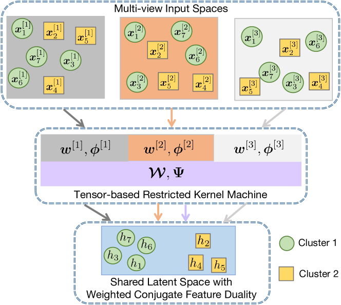
Figure 1: Basic diagram of the proposed method. Data $\bm{x}^{[v]}_{i}$ are mapped into different feature spaces using $\bm{w}^{[v]}$ and $\bm{\phi}^{[v]}$ for each view $v=1,2,3$, and meanwhile tensors $\mathcal{W}$ and $\bm{\Psi}$ integrating all views are modelled, where view-specific information (in grey, orange, and light grey) is retained and high-order correlations between different views are incorporated (in purple). Through the proposed weighted conjugate feature duality with RKM, a shared latent space is attained for spectral clustering, where clusters are well separated and data interpretation analyses are facilitated via the hidden features common to all views.

The contributions of this work mainly include:

• We propose a novel method for MvSC based on the Fenchel-Young inequality, giving an upper bound to the weighted KPCA problem for spectral clustering and introducing dual variables in a different way that leads to an efficient representation and simple optimization.

• As the dual variables play the role of conjugated hidden features in the latent space, we impose shared dual variables on all views to construct a common latent space, realizing the view couplings and facilitating interpretation analysis with dual representations.

• The resulting optimization problem only needs the solution of a single eigenvalue decomposition, whose dimension is independent of the number of views. A tensor-based model is established to capture high-order correlations of the views without increasing computational complexity.

• We discuss the applicability of our method to predict unseen data based on the eigenspace found in training, which also enables to efficiently tackle large-scale data. Numerical experiments verify the superiority of our method in accuracy, efficiency, and interpretation.

The remainder of this paper is organized as follows: Section 2 summarizes the background of MvSC and RKM. In Section 3, the proposed method is presented in detail, including representation models together with derivations, the optimization problem, and discussions. Section 4 presents the experimental results, verifying the advantages of the proposed method from different aspects. In Section 5, brief concluding remarks are given.

2 Background

2.1 Related Work for MvSC

In multi-view learning for spectral clustering (MvSC), data of different views provide complementary information about a common data partitioning underlying all the views. Simply concatenating the attributes of all views with early fusion or combining the single-view learning results with late fusion can give reasonable results, but the performance is far from satisfactory due to the lack of utilizing view couplings [17, 7, 5]. To this end, great efforts have been made on exploring the common intrinsic clustering structure underlying multiple views with varied methodologies.

The co-regularization technique is one of the pioneering methods for MvSC [38, 12, 30], where extra regularization items are introduced to the optimization objective in training. In this way, the final model is trained by simultaneously considering the view-specific modelling parts and also their mutual influence. For example, [12] (Co-reg) deploys a co-regularized loss with either a pairwise or a centroid coupling scheme, and it is commonly considered as one of the baselines; [30] (MvKSC) incorporates pair-wise coupling items with pre-defined weights to the primal objective with LSSVM. Graph-based methods have attracted great popularity for MvSC. They aim to learn a common graph containing clustering information via multiple graphs across views [23, 24, 25, 26]. As a representative method, [15] (COMIC) jointly considers the geometric consistency and the cluster assignment consistency, where the former learns a connection graph for data from the same cluster while the later minimizes the discrepancy of pairwise connection graphs from different views. More recently, [27] (SFMC) efficiently coalesces multiple view-wise graphs, learns the weights, and manipulates the joint graph by a connectivity constraint indicating clusters and the selected anchors. Even though one of the main issues tackled in both COMIC and SFMC is the parameter-free tuning, there still exist settings that should be tuned in order to well cluster varied datasets, e.g., the threshold of estimating clusters in COMIC. Despite the diverse fusion techniques in the aforementioned works, higher-order correlations across views can be further enhanced by using tensor learning. The representative method based on tensor singular value decomposition is [18] (tSVD-MSC), which adopts self-representation coefficients of views to construct the tensor and uses the tensor nuclear norm to learn the optimal subspace by rotating the constructed tensor. It improved clustering performance over many matrix-based methods, but the computational cost increases distinctively.

Recently, several late fusion MvSC methods have been proposed with diversified fusion techniques as well as reduced computational complexity for large-scale data[39]. These methods seek an optimal partition by combing linearly-transformed partitions in individual views and using $k$-means for the learned consensus partition matrix to get cluster labels. In [40] (OP-LFMVC), learning of the consensus partition matrix and generation of cluster labels are unified by developing a four-step alternate algorithm. Similarly, in [41] (OPMC) a one-pass fusion method is proposed, which unifies and jointly optimizes the steps of matrix factorization and partition generation, where an alternate strategy is constructed to obtain the parameters. Additionally, towards large-scale data and computational efficiency, bipartite graphs are effective strategies, as only part of the samples need to be selected to build the graphs in relation to the data structure for clustering. In [28] (MVSCBP), local manifold fusion is used to integrate heterogeneous features and approximate the similarity measures using bipartite graphs with selected salient points, and out-of-sample inference is also considered by label propagations, further improving the efficiency. In SFMC, bipartite graphs are also used to build sample connectivity by selecting anchors [27].

KSC [21] formulates spectral clustering as a weighted KPCA problem with LSSVM[29], where the clustering information is included based on the eigendecomposition of a modified similarity matrix of the data and the random walk model in relation to the graph information is utilized for the weighting [42]. More discussion on the links between spectral clustering and the weighted KPCA can be found in [43, 21]. The solution (stationary points) to KSC is given by an eigenvalue decomposition scaled by $N\times N$. The projections by the weighted KPCA, i.e., clustering scores, are computed by the first eigenvectors and then used to encode the clusters. For multi-view learning, KSC has been analogously extended to MvKSC [30] by imposing additional constraints in the primal model, which yields a $VN\times VN$ eigenvalue problem, where $V$ is the number of views.

2.2 Restricted Kernel Machines

The RKM formulation for KPCA, i.e., the unweighted settings for KSC, is given by an upper bound of the objective function in LSSVM using the Fenchel-Young inequality [44]: $\frac{1}{2\lambda}\bm{\epsilon}^{T}\bm{\epsilon}+\frac{\lambda}{2}\bm{u}^{T}\bm{u}\geq\bm{\epsilon}^{T}\bm{u},\forall\bm{\epsilon},\bm{u}\in\mathbb{R}^{s},$ which introduces the hidden features $\bm{u}$ and leads to the conjugate feature duality. The resulting KPCA objective is given by:

$$\mathcal{J}=-\sum\limits_{i=1}^{N}\bm{\epsilon}_{i}^{T}\bm{u}_{i}+\dfrac{\lambda}{2}\sum\limits_{i=1}^{N}{\bm{u}_{i}}^{T}{\bm{u}_{i}}+\dfrac{\eta}{2}\mathrm{Tr}\left(\bm{W}^{T}\bm{W}\right),$$ (1)

where the hidden features $\bm{u}_{i}$ for each sample are conjugated to the projections $\bm{\epsilon}_{i}=\bm{W}^{T}\bm{\phi}(\bm{x}_{i})$ along all $s$ directions with the interconnection weight $\bm{W}\in\mathbb{R}^{d_{h}\times s}$ and feature map $\bm{\phi}:\mathbb{R}^{d}\rightarrow\mathbb{R}^{d_{h}}$, and $\eta,\lambda\in\mathbb{R}_{+}$ are the regularization constants. Here, the first summation term resembles the energy function of RBM [32], involving connections between visible units in the input space and hidden units in the latent space, as demonstrated in Figure 2.

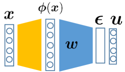
Figure 2: Graphical topology of RKM for KPCA. An input $\bm{x}$ is mapped to a feature space using a feature map ${\bm{\phi}}$ with projections $\bm{\epsilon}$ coupled with hidden features $\bm{u}$ in the latent space.

By characterizing the stationary points of $\mathcal{J}$ in $\eqref{eq:obj:ksc:rkm}$, the following eigenvalue problem is obtained:

$$\frac{1}{\eta}{\bm{\Omega}_{\rm c}}\bm{U}^{T}=\bm{U}^{T}\bm{\Lambda},$$ (2)

where $\bm{U}=[\bm{u}_{1},\ldots,\bm{u}_{N}]\in\mathbb{R}^{s\times N}$ and $\bm{\Lambda}={\rm diag}\{\lambda_{1},\allowbreak\ldots,\allowbreak\lambda_{N}\}$ with $s\leq N$ selected principal components, and ${\bm{\Omega}_{\rm c}}$ is the centered Mercer kernel matrix [45] induced by ${\bm{\phi}}(\cdot)$. One can verify that the solutions corresponding to different eigenvectors and eigenvalues in (2) all lead to $\mathcal{J}=0$ [31].

3 Multi-view Spectral Clustering via Shared Latent Space with RKM

In this section, the model formulation and the optimization of the proposed method are derived. Then, the decision rule for encoding the clusters and the out-of-sample extension are explained.

3.1 Model Formulation

3.1.1 Modified Weighted Conjugate Feature Duality for Spectral Clustering

Under weighted least squares settings, the conjugate feature duality for KPCA with $s$ components in (1) can be extended based on the following inequality:

$$\frac{1}{2\lambda}\bm{\epsilon}^{T}\bm{P}\bm{\epsilon}+\frac{\lambda}{2}\bm{u}^{T}\bm{P}^{-1}\bm{u}\geq\bm{\epsilon}^{T}\bm{u},\quad\forall\bm{\epsilon},\bm{u}\in\mathbb{R}^{s},$$ (3)

with $\bm{P}\succ 0$ and $\lambda>0$ [46], where the hidden features $\bm{u}$ regarding each sample are conjugated to the projections $\bm{\epsilon}$. It can be seen that the use of matrix $\bm{P}\in\mathbb{R}^{s\times s}$ realizes the weighting over the selected $s$ components.

In KSC-based methods, spectral clustering can be formulated as a weighted KPCA problem with LSSVM. The corresponding primal model for the single-view KSC with $k$ clusters is expressed as[21]:

$$\begin{array}[]{lll}\min\limits_{\bm{w}^{{(l)}},\bm{e}^{{(l)}}}&\mathcal{J}_{\rm KSC}=\dfrac{\eta}{2}\sum\limits_{l=1}^{k-1}{\bm{w}^{{(l)}}}^{T}\bm{w}^{{(l)}}-\sum\limits_{l=1}^{k-1}\dfrac{1}{2\lambda^{(l)}}{\bm{e}^{{(l)}}}^{T}\bm{D}^{-1}\bm{e}^{(l)}\\ {\hskip 17.07164pt\rm{s.t.}}&\bm{e}^{{(l)}}=\left(\bm{\Phi}-\mathbf{1}_{N}\hat{\bm{\mu}}^{T}\right)\bm{w}^{(l)},\end{array}$$ (4)

where $\bm{w}^{{(l)}},\bm{e}^{{(l)}}\in\mathbb{R}^{N}$, $l=1,\dots,k-1,\lambda^{(l)}>0$, $\bm{1}_{N}$ denotes a vector with $N$ ones, and $\hat{\bm{\mu}}$ is used to center the data. The matrix $\bm{D}\in\mathbb{R}^{N\times N}$ is the so-called degree matrix constructed in relation to the random walks model [42] and is formulated as a positive definite diagonal matrix with $D_{ii}=\sum\nolimits_{j}K(\bm{x}_{j},\bm{x}_{i})$ and $K:\mathbb{R}^{d}\times\mathbb{R}^{d}\mapsto\mathbb{R}$ being the kernel function. For simplicity, we use ${\bm{\Phi}}_{\rm c}=[{{\bm{\phi}}_{\rm c}(\bm{x}_{1})},\ldots,{{\bm{\phi}}_{\rm c}(\bm{x}_{N})}]^{T}$ to denote the centered feature map $\bm{\Phi}-\mathbf{1}_{N}\hat{\bm{\mu}}^{{[v]}^{T}}$ in the paper. The score variables $\bm{e}^{{(l)}}$ encode the data clusters. Note that a set of $k-1$ binary clustering indicators are sufficient to differentiate $k$ clusters, so that $l=1,\dots,k-1$.

In order to tackle spectral clustering, we firstly develop a modified version of weighted conjugate feature duality, which is essential in constructing the objective function of KSC with RKM. Differently, we introduce the hidden features through the Fenchel-Young inequality, but apply it to the $N$-dimensional vector of score variables $\bm{e}=[e_{1},\dots,e_{N}]^{T}$ with the weighting matrix $\bm{D}$, where the conjugation is conducted along each projection direction of all samples, such that

$$\frac{1}{2\lambda}\bm{e}^{T}\bm{D}^{-1}\bm{e}+\frac{\lambda}{2}\bm{h}^{T}\bm{D}\bm{h}\geq\bm{e}^{T}\bm{h},\quad\forall\bm{e},\bm{h}\in\mathbb{R}^{N},$$ (5)

where the matrix $\bm{D}\in\mathbb{R}^{N\times N}$ achieves the weighting over all $N$ samples to build point-wise connectivity between samples. Then, the upper bound objective $\overline{\mathcal{J}}_{\rm KSC}$ is obtained as:

$$\begin{split}\mathcal{J}_{\rm KSC}=&\dfrac{\eta}{2}\sum\limits_{l=1}^{k-1}{\bm{w}^{{(l)}}}^{T}\bm{w}^{{(l)}}-\sum\limits_{l=1}^{k-1}\dfrac{1}{2\lambda^{(l)}}{\bm{e}^{{(l)}}}^{T}\bm{D}^{-1}\bm{e}^{(l)}\\ \leq&-\sum\limits_{l=1}^{k-1}{\bm{e}^{{(l)}}}^{T}\bm{h}^{(l)}+\sum\limits_{l=1}^{k-1}\dfrac{\lambda^{(l)}}{2}{\bm{h}^{(l)}}^{T}\bm{D}\bm{h}^{(l)}\\ &+\dfrac{\eta}{2}\sum\limits_{l=1}^{k-1}{\bm{w}^{{(l)}}}^{T}\bm{w}^{{(l)}}\triangleq\overline{\mathcal{J}}_{\rm KSC},\end{split}$$ (6)

with conjugated hidden features $\bm{h}^{(l)}=[h_{1}^{(l)},\ldots,h_{N}^{(l)}]^{T}$, $l=1,\ldots,k-1$. Thus, the derived $\overline{\mathcal{J}}_{\rm KSC}$ in (6) formulates the corresponding RKM objective $\overline{\mathcal{J}}_{\rm KSC}$ for the weighted KPCA settings in tackling spectral clustering. By substituting the constraints $\bm{e}^{{(l)}}=\bm{\Phi}_{\rm c}\bm{w}^{(l)}$ into the RKM objective $\overline{\mathcal{J}}_{\rm KSC}$, we have

$$\begin{split}\overline{\mathcal{J}}_{\rm KSC}=&-\sum\limits_{l=1}^{k-1}{\left(\bm{\Phi}_{\rm c}\bm{w}^{(l)}\right)}^{T}\bm{h}^{(l)}+\sum\limits_{l=1}^{k-1}\dfrac{\lambda^{(l)}}{2}{\bm{h}^{(l)}}^{T}\bm{D}\bm{h}^{(l)}\\ &+\dfrac{\eta}{2}\sum\limits_{l=1}^{k-1}{\bm{w}^{{(l)}}}^{T}\bm{w}^{{(l)}},\end{split}$$ (7)

where the first summation term in this RKM establishes the interconnections between visible units from the input space and the hidden units from the latent space.

For multi-view learning with data $\mathcal{D}^{[v]}=\{\bm{x}_{i}^{[v]}\}_{i=1}^{N},v=1,\ldots,V$, the view-specific RKM objective $\mathcal{J}^{[v]}_{\rm RKM}$ of our proposed model in primal is formulated as:

$$\begin{split}\overline{\mathcal{J}}^{[v]}_{\rm KSC}=&-\sum\limits_{l=1}^{k-1}{\left(\bm{\Phi}^{[v]}_{\rm c}\bm{w}^{[v]^{(l)}}\right)}^{T}\bm{h}^{{[v]}^{(l)}}+\sum\limits_{l=1}^{k-1}\dfrac{\lambda^{{(l)}}}{2}{\bm{h}^{{[v]}^{(l)}}}^{T}\bm{D}^{[v]}\bm{h}^{{[v]}^{(l)}}\\ &+\dfrac{\eta}{2}\sum\limits_{l=1}^{k-1}{\bm{w}^{[v]^{(l)}}}^{T}\bm{w}^{[v]^{(l)}}\triangleq\mathcal{J}^{[v]}_{\rm RKM},\end{split}$$ (8)

with score variables (projections) in (4) expanded as

$$\bm{e}^{[v]^{(l)}}=(\bm{\Phi}^{[v]}-\mathbf{1}_{N}\hat{\bm{\mu}}^{{[v]}^{T}})\bm{w}^{[v]^{(l)}}\triangleq\bm{\Phi}^{[v]}_{\rm c}\bm{w}^{[v]^{(l)}},$$ (9)

where $\bm{h}^{{[v]}^{(l)}}\in\mathbb{R}^{N}$ are the conjugated hidden features in the induced latent space of the $v$-th view, $\bm{\Phi}^{[v]}=[\bm{\phi}^{[v]}(\bm{x}^{[v]}_{1}),\ldots,\bm{\phi}^{[v]}(\bm{x}^{[v]}_{N})]^{T}\in\mathbb{R}^{N\times d_{h}}$ contains the view-specific feature maps $\bm{\phi}^{[v]}:\mathbb{R}^{d^{[v]}}\rightarrow\mathbb{R}^{d_{h}^{[v]}}$ with interconnection weight $\bm{w}^{[v]^{(l)}}\in\mathbb{R}^{d_{h}^{[v]}}$, and $\bm{\Phi}^{[v]}_{\rm c}$ denotes the corresponding centered feature map. Analogously, $\bm{D}^{[v]}\in\mathbb{R}^{N\times N}$ is the degree matrix for the $v$-th view.

In the constructed RKM objective $\mathcal{J}^{[v]}_{\rm RKM}$ of KSC, the first two sets of summation terms give the view-specific connections between the inputs and the hidden units of the latent space.

3.1.2 Shared Latent Space

Under the RKM learning framework, we start from weighted KPCA and introduce a modified conjugate feature duality to formulate the RKM objective $\mathcal{J}^{[v]}_{\rm RKM}$ for spectral clustering in each view, as shown in Section 3.1.1. For multiple views, we simultaneously incorporate the view-specific RKM objectives of KSC, leading to the objective:

$$\begin{split}\mathcal{J}_{\rm Mv}=&\sum\limits_{v=1}^{V}\mathcal{J}^{[v]}_{\rm RKM}.\end{split}$$ (10)

Importantly, we impose the couplings of different views by sharing hidden features in the latent space, due to the conjugate dual variables being hidden features in RKM. Thus, in the context of this paper, the sharing of hidden features in the induced common latent space is achieved by

$$\bm{h}^{{[1]}^{(l)}}=\cdots=\bm{h}^{{[V]}^{(l)}}\triangleq\bm{h}^{{(l)}}.$$ (11)

Figure 3 gives the graphical topology and shows that the learned features from the spaces of different views are projected into the common latent space, which well retains the view-specific information and meanwhile jointly considers the mutually shared information of all views. The constructed common latent space perfectly fits and facilitates the goal of our task, i.e., finding the common data partitions for all views, as we can learn a shared representation of the data from all views and promote the clustering in the latent space. Analysis can also be simplified for all views, providing a more straightforward way for interpretation and data discovery in such common latent space with dual representations.

Figure 3: Graphical topology of the shared latent space with RKM. Each view $v$ is mapped to a feature space using a feature map ${\bm{\phi}}^{[v]}$ with view-specific projections ${{\bm{e}}^{[v]}}^{(l)}$, where the degree matrix $\bm{D}^{[v]}$ is in relation to the random walks model promoting the clustering. The couplings between views are obtained by deploying the conjugated hidden features ${\bm{h}}^{(l)}$ in the common latent space, shared by all views.

3.1.3 Tensor-based modelling

Though the shared hidden features in the latent space can lead to the couplings of all views, the feature maps $\bm{\phi}^{[v]}$ and their interconnection weights $\bm{w}^{{[v]}^{(l)}}$ are still calculated separately for individual views, as shown in Figure 3. To boost high-order correlations, we incorporate tensor learning to our model, which extends the fusion strategy and further explores the complementary information across views.

In the objective, we introduce multi-order weight tensors and rank-1 feature mapping tensors to build the model, instead of using view-specific matrices and vectors. Thus, the full objective using tensor representations is attained as:

$$\begin{split}\mathcal{J}_{\rm TMv}=&-\sum\limits_{l=1}^{k-1}\sum\limits_{i=1}^{N}\left<{{\bm{\Psi}}}_{{\rm c},i},{\mathcal{W}}^{(l)}\right>h^{{(l)}}_{i}+\\ &\sum\limits_{v=1}^{V}\sum\limits_{l=1}^{k-1}\dfrac{\lambda^{(l)}}{2}{\bm{h}^{{(l)}}}^{T}\bm{D}^{[v]}\bm{h}^{{(l)}}+\dfrac{\eta}{2}\sum\limits_{l=1}^{k-1}\left<\mathcal{W}^{(l)},\mathcal{W}^{(l)}\right>,\end{split}$$ (12)

where $\mathcal{W}^{(l)}\in\mathbb{R}^{d_{h}^{{[1]}}\times\cdots\times d_{h}^{{[V]}}}$ are $V$-th order tensors of the interconnection weights for the $l$-th projection, ${\bm{\Psi}}_{{\rm c},i}\in\mathbb{R}^{d_{h}^{{[1]}}\times\cdots\times d_{h}^{{[V]}}}$ are rank-1 tensors composed by the outer products of all view-specific feature maps, such that ${\bm{\phi}}_{\rm c}^{[1]}(\bm{x}_{i}^{[1]})\otimes\cdots\otimes{\bm{\phi}}_{\rm c}^{[V]}(\bm{x}_{i}^{[V]})$. The outer product and the tensor inner product are calculated by $\mathcal{A}_{{m_{1}}\ldots{m_{P}}}\coloneqq\bm{a}_{1_{m_{1}}}\otimes\cdots\otimes\bm{a}_{P_{m_{P}}}$ and $\left<\mathcal{A},\mathcal{B}\right>\coloneqq\sum\nolimits_{m_{1}=1}^{M_{1}}\cdots\sum\nolimits_{m_{p}=1}^{M_{P}}\mathcal{B}_{{m_{1}}\ldots{m_{P}}}\mathcal{A}_{{m_{1}}\ldots{m_{P}}}$, respectively, with $P$ vectors $\bm{a}_{1}\in\mathbb{R}^{M_{1}},\ldots,\bm{a}_{P}\in\mathbb{R}^{M_{P}}$ for the outer product and two $P$-th order tensors $\mathcal{A},\mathcal{B}\in\mathbb{R}^{M_{1}\times\cdots\times M_{P}}$ for the inner product. Note that, as $\bm{h}^{(l)}$ is shared by all views, the calculations between $\bm{h}^{(l)}$ and degree matrix $\bm{D}^{[v]}$ in the second summation term remain the same.

The constructed tensors ${\bm{\Psi}}_{{\rm c},i}$ and $\mathcal{W}^{(l)}$ join the feature maps and interconnection weights, respectively, of all views together. Figure 4 shows the graphical topology of the proposed tensor learning, which incorporates the view-specific feature maps within the tensors and performs the calculations of all views simultaneously, leading to the tensor-based high-order couplings and information fusion in an earlier stage compared to Figure 3, which, by contrast, fuses the views in a relatively later stage.

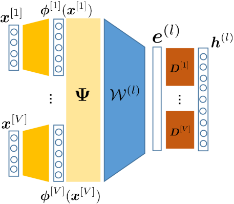
Figure 4: Graphical topology of the tensor-based model. All views are mapped to a feature tensor ${\bm{\Psi}}$ constructed by the outer product of the feature maps ${\bm{\phi}}^{[v]}$ of all views. Then, the fused information is connected by the weight tensors $\mathcal{\bm{W}}^{(l)}$ with the conjugated hidden features ${\bm{h}}^{(l)}$ in the common latent space.

With the shared latent space and tensor learning, we then generalize the proposed model, namely TMvKSCR, extending to weighted views and integrated fusions. Firstly, we integrate the matrix (later fusion in Figure 3) and the tensor (earlier fusion in Figure 4) representations by combining $\mathcal{J}_{\rm Mv}$ and $\mathcal{J}_{\rm TMv}$, for diversified couplings and fusions. Secondly, we consider a more general case where the relative impacts of different views can be varied, for example the reliability (noise) varies in different views. Thus, the clustering scores from different views are weighted in $\mathcal{J}^{[v]}_{\rm RKM}$ by replacing $\bm{e}^{{[v]}^{(l)}}$ with $\sqrt{\kappa^{[v]}}\bm{e}^{{[v]}^{(l)}}$, where the yielded objective is denoted $\mathcal{J}_{\rm RKM}^{{\kappa}^{[v]}}$. Note that the weighted outer product involving the tensors in $\mathcal{J}_{\rm TMv}$ is equivalent to an amplification magnitude of $\sqrt{\kappa^{[1]}\cdots\kappa^{[V]}}$ without changing the solution space.

Accordingly, our model generalized in this paper, i.e., TMvKSCR, is given by the following objective:

$$\mathcal{J}_{\rm TMvR}=\varrho\sum\limits_{v=1}^{V}\mathcal{J}_{\rm RKM}^{{\kappa}^{[v]}}+(1-\varrho)\mathcal{J}_{\rm TMv}.$$ (13)

In our model, we learn projections of multi-view data into the common latent space by sharing the conjugated dual variables (hidden features) in RKM, and the tensor learning further boosts high-order correlations across views, incorporating the global inter-view information. At the same time, the view-specific information is well retained by the individual feature maps of weighted views, incorporating the local intra-view information. Therefore, the intra-view relations and the inter-view correlations are both explored.

3.2 Problem Optimization

In the optimization, instead of tackling the explicit feature maps $\bm{\phi}^{[v]}$ in in primal representations, we consider characterizing the stationary points of $\mathcal{J}_{\rm TMvR}$ with conjugate feature duality [31] and the kernel trick [47].

By taking the partial derivatives to the weights and the hidden features, the conditions of the stationary points for $\mathcal{J}_{\rm TMvR}$ are characterized by:

$$\left\{\begin{split}\dfrac{\partial\mathcal{J}_{\rm TMvR}}{\partial\bm{w}^{[v]^{(l)}}}=&\eta\bm{w}^{[v]^{(l)}}-\sqrt{\kappa^{[v]}}\sum\limits_{i=1}^{N}{\bm{\phi}}_{\rm c}^{[v]}\left(\bm{x}_{i}^{[v]}\right)h_{i}^{(l)}=0,\\ \dfrac{\partial\mathcal{J}_{\rm TMvR}}{\partial\mathcal{W}^{(l)}_{m_{1}\ldots m_{V}}}=&\eta\mathcal{W}^{(l)}_{m_{1}\ldots m_{V}}-\sum\limits_{i=1}^{N}\prod\limits_{v=1}^{V}{\bm{\phi}}_{\rm c}^{[v]}\left(\bm{x}_{i}^{[v]}\right)_{m_{v}}h_{i}^{(l)}=0,\\ &\text{with}\ m_{v}=1,\ldots,d^{[v]}_{h},\\ \dfrac{\partial\mathcal{J}_{\rm TMvR}}{\partial h_{i}^{(l)}}=&\varrho\sum\limits_{v=1}^{V}\sqrt{\kappa^{[v]}}{\bm{w}^{[v]^{(l)}}}^{T}{\bm{\phi}}_{\rm c}^{[v]}\left(\bm{x}_{i}^{[v]}\right)\\ &+(1-\varrho)\left<{{\bm{\Psi}}}_{{\rm c},i},\mathcal{\bm{W}}^{(l)}\right>-\sum\limits_{v=1}^{V}\lambda^{(l)}D_{ii}^{[v]}h_{i}^{(l)}=0,\\ &\text{with}\ i=1,\ldots,N,\end{split}\right.$$ (14)

for $l=1,\ldots,k-1$. From the first two equations in (14), it follows:

$$\left\{\begin{array}[]{ll}\bm{w}^{[v]^{(l)}}=\dfrac{1}{\eta}\sqrt{\kappa^{[v]}}\sum\limits_{i=1}^{N}{\bm{\phi}}_{\rm c}^{[v]}\left(\bm{x}_{i}^{[v]}\right)h_{i}^{(l)},\\ \mathcal{W}^{(l)}_{m_{1}\ldots m_{V}}=\dfrac{1}{\eta}\sum\limits_{i=1}^{N}\prod\limits_{v=1}^{V}{\bm{\phi}}_{\rm c}^{[v]}\left(\bm{x}_{i}^{[v]}\right)_{m_{v}}h_{i}^{(l)}.\end{array}\right.$$ (15)

Eliminating $\bm{w}^{[v]^{(l)}}$ and $\mathcal{W}^{(l)}_{m_{1}\ldots m_{V}}$ gives the following expression in the conjugated features $h^{(l)}_{i}$,

$$\begin{split}&\dfrac{1-\varrho}{\eta}\prod\limits_{v=1}^{V}\sum_{m_{v}=1}^{d_{h}^{[v]}}{\bm{\phi}}_{\rm c}^{[v]}\left(\bm{x}_{i}^{[v]}\right)_{m_{v}}\left(\sum\limits_{j=1}^{N}\prod\limits_{v=1}^{V}{\bm{\phi}}_{\rm c}^{[v]}\left(\bm{x}_{j}^{[v]}\right)_{m_{v}}h_{j}^{(l)}\right)\\ &+\dfrac{\varrho}{\eta}\sum\limits_{v=1}^{V}{\kappa^{[v]}}\sum\limits_{j=1}^{N}{\bm{\phi}}_{\rm c}^{[v]}\left(\bm{x}_{j}^{[v]}\right)^{T}{\bm{\phi}}^{[v]}_{\rm c}\left(\bm{x}_{i}^{[v]}\right)h_{j}^{(l)}=\lambda^{(l)}\sum\limits_{v=1}^{V}D_{ii}^{[v]}h_{i}^{(l)},\\ &{\text{for}\ l=1,\ldots,k-1,\ \text{and}\ i=1,\ldots,N,}\end{split}$$ (16)

yielding the following eigenvalue problem (17) for the optimization of our method

$$\begin{split}&\dfrac{1}{\eta}\left(\sum\limits_{v=1}^{V}\bm{D}^{[v]}\right)^{-1}\left(\varrho\sum\limits_{v=1}^{V}\kappa^{[v]}{\bm{\Omega}}_{\rm c}^{[v]}+\left(1-\varrho\right)\bigodot_{v=1}^{V}{\bm{\Omega}}_{\rm c}^{[v]}\right)\bm{H}\\ &\hskip 99.58464pt=\bm{H}\bm{\Lambda},\end{split}$$ (17)

where ${\bm{\Omega}}_{\rm c}^{[v]}={\bm{\Phi}}_{\rm c}^{{[v]}}{{\bm{\Phi}}_{\rm c}^{{[v]}}}^{T}$ denotes the centered kernel matrix induced by the kernel function $K^{[v]}:\mathbb{R}^{d^{[v]}}\times\mathbb{R}^{d^{[v]}}\rightarrow\mathbb{R}$, and $\bm{H}\coloneqq[\bm{h}^{(1)},\ldots,\bm{h}^{(k-1)}]\in\mathbb{R}^{N\times(k-1)}$ contains the selected $k-1$ components (eigenvectors) corresponding to the largest $k-1$ eigenvalues $\bm{\Lambda}\coloneqq{\rm diag}\{\lambda^{(1)},\allowbreak\ldots,\allowbreak\lambda^{(k-1)}\}$. By solving (17), the first $k-1$ eigenvectors are used to calculate the score variables $\bm{e}^{{[v]}^{(l)}}$ for clustering. Note that $\eta$ is a scaling factor without affecting the solution space of the optimization problem and thereby set as 1.

It can be seen from (17) that, although the proposed model integrates both view-wise information and high-order correlations across all views into a common latent space with dual representations, the resulting optimization is simple in formulation, i.e., solving an $N\times N$ eigenvalue decomposition problem for the first $k-1$ eigenvectors, which gives the stationary points of the objective function $\mathcal{J}_{\rm TMvR}$ as derived in (14). Thus, the optimization procedure of our method does not need to iteratively alternate updating model parameters, which instead is commonly required in many related works including subspace and graph-based methods, e.g., [28, 15, 40, 19, 20, 41, 27]. Moreover, the scale of (17) is independent of the number of views $V$, and this efficiency owes to the shared hidden features of all views with the conjugate feature duality in RKM, so that there is no need to expand the size of dual variables along with the increasing number of views.

The clustering score variables $\bm{e}^{[v]^{(l)}}$ in (9) can then be computed using the kernel trick in dual form. Accordingly, the dual model representation for the score variables corresponding to each data point is calculated by

$$\hat{e}^{{[v]}^{(l)}}_{i}(\bm{x}^{[v]}_{i})=\sum\limits_{j=1}^{N}h^{(l)}_{j}K^{[v]}(\bm{x}_{i}^{[v]},\bm{x}_{j}^{[v]}).$$ (18)

With the $k-1$ eigenvectors obtained from (17), i.e., $\bm{h}^{(l)}=[h_{1}^{(l)},\ldots,h_{N}^{(l)}]^{T}$ for $l=1,\ldots,k-1$, the score variables of all data points are obtained and their cluster labels can be encoded accordingly, as explained in Section 3.3.

3.3 Decision Rule and Out-of-Sample Extension

The encoding vector of a certain sample from multiple views $\{\bm{x}_{i}^{[v]}\}_{v=1}^{V}$ consists of the indicators:

$${\rm sign}\left(e_{i}^{{[v]}^{(1)}}\right),\dots,{\rm sign}\left(e_{i}^{{[v]}^{(k-1)}}\right),$$ (19)

where the score variables are calculated in the dual form by $\bm{e}^{{[v]}^{(l)}}={\bm{\Omega}}_{\rm c}^{[v]}\bm{h}^{(l)}$ in (18). The $k$ most occurring encoding vectors form the codebook. In multi-view cases, the clustering assignment can be done in two ways: individual assignment and ensemble assignment. For the former, the cluster assignment can be done separately for each view, and $V$ codebooks are created, i.e., $\mathcal{C}^{[v]}=\{c_{p}^{[v]}\}_{p=1}^{k}$. These clustering results can vary across views. For the latter, which we use in this paper, a single cluster assignment is conducted for all views by $\bm{e}^{(l)}_{\rm mean}=\sum\nolimits_{v=1}^{V}\beta^{[v]}\bm{e}^{{[v]}^{(l)}}$, where only one codebook $\mathcal{C}=\{c_{p}\}_{p=1}^{k}$ is created and $\beta^{[v]}$ can be simply taken as $1/V$ or calculated separately. Each data point is then assigned to the cluster of the closest codeword based on the ECOC decoding [48].

The proposed method can be flexibly applied to cluster unseen data, i.e., the out-of-sample extension, a merit from KSC-related techniques [49]. Similar to (18), the scores for unseen data $\mathcal{D}^{[v]}_{\rm test}=\{{\bm{x}^{[v]}_{\rm test}}_{j}\}_{j=1}^{N_{\rm te}}$ can be calculated to correspond to the projections onto the eigenvectors found in the training, i.e.,

$$\bm{e}^{{[v]}^{(l)}}_{\rm test}={\bm{\Omega}}_{\rm c,test}^{[v]}{\bm{h}^{(l)}},$$ (20)

where ${\bm{\Omega}}_{\rm c,test}^{[v]}\in\mathbb{R}^{N_{\rm te}\times N}$ is the centered testing kernel matrix computed from $\bm{\Omega}_{{\rm test}_{ij}}^{[v]}=K^{[v]}(\bm{x}_{{\rm test}_{i}}^{[v]},\bm{x}_{j}^{[v]})$. Hence, we do not need to re-conduct the training procedure when new data are included, which is particularly useful in dealing with large-scale data. For instance, the fixed-size kernel scheme [50] can be applied in our method using dual representations, as a small subset of data is selected for the training, and then the clusters of the complete dataset can be inferred by using out-of-sample extensions. Algorithm 1 details the training and the out-of-sample extension of the proposed method.

Algorithm 1 Training and Out-of-sample Inference Procedures of the Proposed TMvKSCR

1:  Input: $\mathcal{D}^{[v]}=\{\bm{x}_{i}^{[v]}\}_{i=1}^{N}$ and $\mathcal{D}^{[v]}_{\rm test}=\{{\bm{x}^{[v]}_{\rm test}}_{j}\}_{j=1}^{N_{\rm te}}$ (if present), $K^{[v]}(\cdot,\cdot)$, $k$, $\kappa^{[v]}$ and $\varrho$;

2:  Output: Clusters of data.

3:  Compute the centered kernel matrices ${\bm{\Omega}}_{\rm c}^{[v]}$ and their degree matrices $\bm{D}^{[v]}$;

4:  Solve the eigenvalue problem in (17) and obtain $\bm{h}^{(l)}$;

5:  Compute the score variables $\bm{e}^{{[v]}^{(l)}}$ by (18) and build the codebook $\mathcal{C}=\{c_{p}\}_{p=1}^{k}$, with $c_{p}\in\{-1,1\}^{k-1}$;

6:  Assign each $\bm{x}_{i}^{[v]}$ to its cluster by applying the codebook $\mathcal{C}$ on ${\rm sign}(\bm{e}^{{[v]}^{(1:k-1)}}_{i})$ of (19);   $\triangleright$ Clusters of $\mathcal{D}^{[v]}$

7:  if $\mathcal{D}^{[v]}_{\rm test}\neq\emptyset$ then

8:     Compute the centered kernel matrices ${\bm{\Omega}}_{\rm c,test}^{[v]}$;

9:     Compute the score variables $\bm{e}_{\rm test}^{{[v]}^{(l)}}$ by (20);

10:     Assign each ${\bm{x}^{[v]}_{\rm test}}_{j}$ to its cluster by applying codebook $\mathcal{C}$ on ${\rm sign}(\bm{e}^{{[v]}^{(1:k-1)}}_{i})$ of (19);  $\triangleright$ Clusters of $\mathcal{D}_{\rm test}^{[v]}$

11:  end if

3.4 Computational Complexity Analysis

The computation involved in the proposed TMvKSCR mainly covers two aspects, i.e., obtaining the kernels and calculating the first $k-1$ eigenvectors in (17). Denoting the average input dimensions of all views as $\overline{d}=(1/V)\sum_{v=1}^{V}d^{[v]}$, the first aspect of kernel computation has a time complexity of $\mathcal{O}(VN^{2}\overline{d})$[51], which is commonly involved in spectral clustering methods when calculating the similarity matrices consisting of the point-wise relations between samples. The second aspect of solving the first $k-1$ eigenvectors in (17) gives a time complexity of $\mathcal{O}((k-1)N^{2})$, which is independent of the number of views $V$ thanks to the shared latent space and leads to the storage complexity as $\mathcal{O}(N^{2})$.

Employing the out-of-sample extension, unseen data can be predicted and analogously the fixed-size kernel scheme can be applied for large-scale data. We assume that $m$ samples are used in the training. The time complexity of the aforementioned two aspects is reduced to $\mathcal{O}(Vm^{2}\overline{d})$ and $\mathcal{O}((k-1)m^{2})$, respectively, with $m\ll N$ and possibly even $m<\overline{d}$. Then, the out-of-sample extension to predict the whole dataset needs the complexity of $\mathcal{O}(VmN\overline{d})$. In this case, the maximal storage complexity is only $\mathcal{O}(m^{2})$. Thus, the main computation is approximately quadratic in the number of samples used for training. Using fixed-size kernels schemes with $m\ll N$ (possibly with $m<\overline{d}$), the proposed method can efficiently deal with large-scale data. Note that our method does not alternate to update parameters with multiple iterations, so it has a fixed complexity, which further helps efficiency.

4 Numerical Experiments

In this section, numerical experiments are conducted to evaluate the proposed method, with comparisons to other related methods on various datasets. Experiments are implemented on MATLAB 2020a/Python 3.7 with 64 GB RAM and a 3.7 GHz Intel i7 processor. More experimental details are supplemented in Appendix A, and the source code can be downloaded from https://github.com/taralloc/mvksc-rkm.

4.1 Experimental Setups

Datasets To evaluate the proposed method, two synthetic datasets (Synth 1/2) are presented, where samples are generated by two-dimensional Gaussian mixture models. For high-dimensional real-world data, we consider the multi-view benchmarks of 3Sources [52], Reuters [53], Ads [54, 14], Image Caption (ImgC) [55], YouTube Video Games (YT-VG) [56], and NUS-WIDE (NUS) [57]. The large-scale Reuters (L-Reuters) [58] is then used to evaluate the out-of-sample extension and the large-scale case, as introduced in Table I, where more details of the datasets are given in Appendix A.

TABLE I: Description of datasets used for the experiments.

Dataset	$N$	$V$	$k$	$d^{[1:V]}$
Synth 1	1000	3	2	2,2,2
Synth 2	1000	2	2	2,2
3Sources	169	3	6	3560, 3631, 3068
Reuters	600	3	6	9749, 9109, 7774
Ads	3279	3	2	587, 495, 472
ImgC	1200	3	3	768, 192, 3522
YT-VG	2100	3	7	1000, 512, 2000
NUS	5970	5	10	64, 225, 144, 73, 128
L-Reuters	18758	5	6	21531, 24892, 34251, 15506, 11547

Evaluation metrics and compared methods To assess the clustering performances of different methods, Adjusted Rand index (ARI) [59] and Normalized Mutual Information (NMI) [60] are widely used to measure the clustering consistency between the true labels and the predicted ones. The ARI metric takes values in $[-1,1]$, with 0 indicating a random partitioning and 1 indicating the perfect clustering identical to the ground truth. The NMI metric normalizes the cluster entropy to give the mutual information between the obtained clustering and the ground-truth clustering. It takes values in $[0,1]$, where 1 indicates the perfect clustering.

We evaluate our proposed TMvKSCR with comparisons to different related methods for MvSC. Firstly, the late fusion based on the best view of view-specific KSC (best) and the early fusion based on attribute concatenation in KSC (concat) are tested. Then, several representative and more recent MvSC methods are compared, including Co-reg [12], MVSCBP[28], tSVD-MSC [18], MvKSC[30], COMIC[15], OP-LFMVC[40], OPMC[40], and SFMC[27], details of which are in Section 2.1. Regarding hyperparameter selection, we tune the hyperparameters of each tested method by grid search in the ranges suggested by the authors in their papers. Though some methods provide a parameter-free setting by using heuristically estimated values, some hyperparameters still need to be tuned to achieve desirable performance on the datasets used in the experiments, such as the clustering threshold in COMIC, the kernels in OP-LFMVC, and the number of salient points and nearest neighbors in MVSCBP. Thus, we also tune such hyperparameters or use the suggested values in the papers of these compared methods and report the obtained optimal results for each dataset. The shared hyperparameters among all methods are tuned under the same settings, e.g., kernel parameters of the RBF bandwidth, and the method-specific hyperparameters, e.g., $\kappa^{[v]}$ and $\varrho$ in our method, are tuned in separate ranges. More details of the setups can be found in Appendix A.

4.2 Performance Comparisons

4.2.1 Clustering Performance

As a simple illustration, Figure 5 plots the score variables of our method and of KSC on the synthetic dataset Synth 1, where the colors represent the two clusters. It shows that the projections of KSC applied to each view cannot find a good separation, while the two groups found by our method are well separated. The improved separation between the clusters leads to better quantitative clustering performance, as shown in Tables II and III.

Figure 5: Score variables for Synth 1 with RBF ($\sigma^{2}=0.05$).

TABLE II: Clustering performance comparisons in terms of the best ARI.

Method	Synth 1	Synth 2	3Sources	Reuters	Ads	ImgC	YT-VG	NUS
KSC (best)	0.678	0.336	0.647	0.194	0.433	0.434	0.030	0.026
KSC (concat)	0.996	0.316	0.688	0.217	0.178	0.351	0.259	0.046
Co-Reg	0.996	0.324	0.655	0.219	0.272	0.471	0.024	0.056
tSVD-MSC	0.817	0.002	0.690	0.248	-0.001	0.637	0.396	0.050
MvKSC	0.996	0.507	0.642	0.233	0.433	0.794	0.205	0.050
COMIC	0.168	0.072	0.489	0.073	0.037	0.511	0.055	0.037
OP-LFMVC	0.988	0.064	0.649	0.231	0.241	0.772	0.388	0.056
OPMC	0.972	0.315	0.321	0.197	0.326	0.430	0.239	0.040
SFMC	0.968	0.236	0.377	0.105	0.223	0.578	0.406	0.021
MVSCBP	0.996	0.322	0.698	0.244	0.366	0.609	0.336	0.050
TMvKSCR	1.000	0.568	0.717	0.273	0.463	0.884	0.526	0.070

TABLE III: Clustering performance comparisons in terms of the best NMI.

Method	Synth 1	Synth 2	3Sources	Reuters	Ads	ImgC	YT-VG	NUS
KSC (best)	0.639	0.289	0.614	0.295	0.344	0.478	0.051	0.033
KSC (concat)	0.989	0.161	0.681	0.311	0.143	0.385	0.324	0.072
Co-Reg	0.989	0.273	0.688	0.347	0.215	0.541	0.050	0.095
tSVD-MSC	0.737	0.001	0.750	0.353	0.039	0.674	0.467	0.080
MvKSC	0.989	0.373	0.669	0.318	0.333	0.739	0.285	0.071
COMIC	0.116	0.166	0.600	0.272	0.127	0.548	0.402	0.095
OP-LFMVC	0.970	0.071	0.645	0.350	0.097	0.748	0.431	0.087
OPMC	0.939	0.259	0.477	0.320	0.154	0.525	0.329	0.083
SFMC	0.936	0.206	0.469	0.388	0.223	0.627	0.654	0.136
MVSCBP	0.989	0.266	0.695	0.397	0.289	0.659	0.555	0.081
TMvKSCR	1.000	0.428	0.756	0.350	0.350	0.835	0.686	0.089

For real-world multi-view datasets, Table II and Table III give the performance evaluation with comparisons to other baselines and state-of-the-art methods. Our method distinctively improves over KSC and MvKSC on all considered datasets regarding both ARI and NMI, showing the effectiveness of our novel fusion technique with the RKM framework. Compared to other approaches, our method achieves the best overall performance on the tested datasets. More specifically, the ARI attained by our method on ImgC is 0.884, compared to the second-best of 0.794 by MvKSC. On YT-VG, our method with a simple linear kernel gives an approximately 32.8% improvement in ARI compared to the second best tSVD-MSC, which also uses tensor learning but is considerably more computationally expensive. COMIC commonly gives much higher NMI than ARI, and this is likely due to NMI not being adjusted for chance, since COMIC automatically determines $k$, which might be overestimated, e.g., it gives 570 clusters for NUS. In such cases, NMI can be very high even with random partitions [61, 62], but the actual clustering is poor. Our method also outperforms the recently proposed SFMC, except for slightly lower NMI on Reuters. For NUS, we only use $m=1000$ samples for the training and infer the remaining data using out-of-sample extensions based on the eigenvectors optimized in training, and our method still achieves the highest ARI and the second highest NMI, showing the effectiveness of the out-of-sample predictions in our method in well balancing accuracy and efficiency. Overall, our method gains the highest ARI on all datasets and maintains the best NMI for most datasets, verifying the efficacy of the proposed tensor-based model and the shared latent space by leveraging conjugate feature duality.

4.2.2 Efficiency

Efficiency comparisons are also conducted to evaluate our method. In this experiment, we compare the running time for all tested methods, and list the corresponding results in Table IV, where the most efficient multi-view method is underlined. Thanks to the shared latent space, our method shows similar running time with single-view methods, i.e., KSC (best/concat), and gives comparable efficiency as OP-LFMVC, which is efficiently designed for large-scale data but shows lower overall accuracy on most datasets in Tables II and III. Compared to other methods, our method is distinctively more efficient. For example, compared to the tensor-based tSVD-MSC that attains the second best overall performance but is the most computationally expensive, our method gives higher performance in considerably less time. When using fixed-size kernel schemes ($m=1000$) with random selection for the larger dataset NUS, our method gains the highest ARI (0.070) in $\approx$0.5s, which is an order of magnitude faster than OP-LFMVC ($\approx$7s).

TABLE IV: Average training time of 10 runs (in seconds).

Method	3Sources		Reuters	Ads	ImgC	YT-VG	NUS
KSC (best)	0.15		0.28	2.34	1.91	1.51	9.50
KSC (concat)	0.17		0.28	4.28	0.52	1.46	10.52
Co-Reg	0.44		1.42	21.42	2.01	7.58	143.55
tSVD-MSC	3.61		55.17	458.48	51.53	152.35	5480.66
MvKSC	0.23		1.68	34.08	19.26	8.15	892.76
COMIC	1.36		19.51	17.94	8.25	18.06	100.77
OP-LFMVC	0.64		0.66	1.14	0.75	1.27	7.19
OPMC	4.09		12.58	7.65	4.05	15.85	30.49
SFMC	0.556		1.311	15.116	2.510	6.555	28.703
MVSCBP	1.848		2.047	9.727	3.372	4.147	9.065
Ours	0.14		0.27	4.47	0.57	1.58	0.50

As introduced before, our method can be implemented with out-of-sample extensions, which greatly benefit large-scale cases, e.g., selecting a subset $m\ll N$ for the training and then inferring the remaining data. To further verify these points, we compare to the methods, i.e., KSC (concat) [21], MvKSC [30], MVSCBP[28], that are extendable to unseen data on both NUS and L-Reuters. In Figure 6, we firstly evaluate the out-of-sample extension in the proposed method on NUS with random subset selection, but selection can also be done with other strategies, e.g., using Renyi entropy [63] or anchor selections [28, 27]. Our method maintains higher ARI and NMI on varying $m$. It can also be observed that our method shows negligible performance degradation to the full accuracy on NUS, when only $1/3$ of the complete data are randomly selected and used in training, further verifying the informativeness of hidden features found in our method.

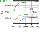
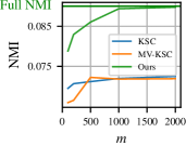
Figure 6: ARI and NMI on NUS with varied $m$ averaged over 10 runs. Given the same $m$, MvKSC using Lagrangian duality tackles a $5m\times 5m$ eigenvalue problem, while our method maintains higher ARI and NMI by solving an $m\times m$ one instead, which is of particular benefit under limited computational resources.

We further compare with the scalable MVSCBP, OP-LFMVC, and SFMC on L-Reuter dataset. Consistent with the settings used in the compared papers [28, 27], $m=400$ salient points, or namely the anchors, are used in building the graphs for training; we use the same $m=400$ salient points in our training phase. The comparison results on accuracy and efficiency are given in Table V. It can be seen that our method achieves competitive performance than the compared methods, attaining the highest ARI. It is worth mentioning that our method shows distinctively less CPU time, where the running time is reduced by more than $1\sim 2$ orders of magnitude than the compared scalable methods, showing the efficiency of the out-of-sample extension in the proposed method and its effectiveness for large-scale cases.

TABLE V: Clustering performance and running time (in seconds) on L-Reuters.

	ARI	NMI	Time
MVSCBP	0.270	0.339	3.88
OP-LFMVC	0.257	0.317	48.54
SFMC	0.126	0.341	58.15
Ours	0.312	0.312	0.29

4.3 Further Analysis and Interpretation

Leveraging the shared latent space with dual representations in RKM provides versatile perspectives on clustering interpretation and analysis in a more straightforward way. We can conduct analysis directly on the constructed model itself to reveal the clustering results without external tools.

4.3.1 Eigenvalues

The selected eigenvectors corresponding to the largest eigenvalues in (17) are used for clustering and play a significant role in the performance. We investigate the largest eigenvalues: Figure 7 plots the percentage of explained variance and the cumulative variance for Synth 1, where KPCA and KSC are applied with attribute concatenation.

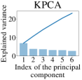
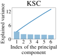
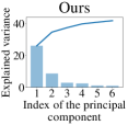
Figure 7: Explained variance for Synth 1. Our method captures more information with fewer components and brings a more informative largest component along with a sharper eigenvalue decay.

In Figure 7, the eigenvalue drops distinctively after the first component in all plots, where our method shows the sharpest decay. This dataset has two clusters, so the first eigenvector is sufficient for binary clustering. The percentage of explained variance by the first component in our method is around 25%, compared to less than 8% in KPCA and 5% in KSC. The advantage of KSC is not distinctive over KPCA here, though KSC employs the degree matrix to introduce the clustering information. This experiment shows that our method indeed leads to more informative components, ultimately resulting in more separable clusters. For real-world data, an analogous analysis can be performed, where Ads is illustrated and comparisons to MvKSC are also given in Figure 8, showing similar results.

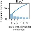
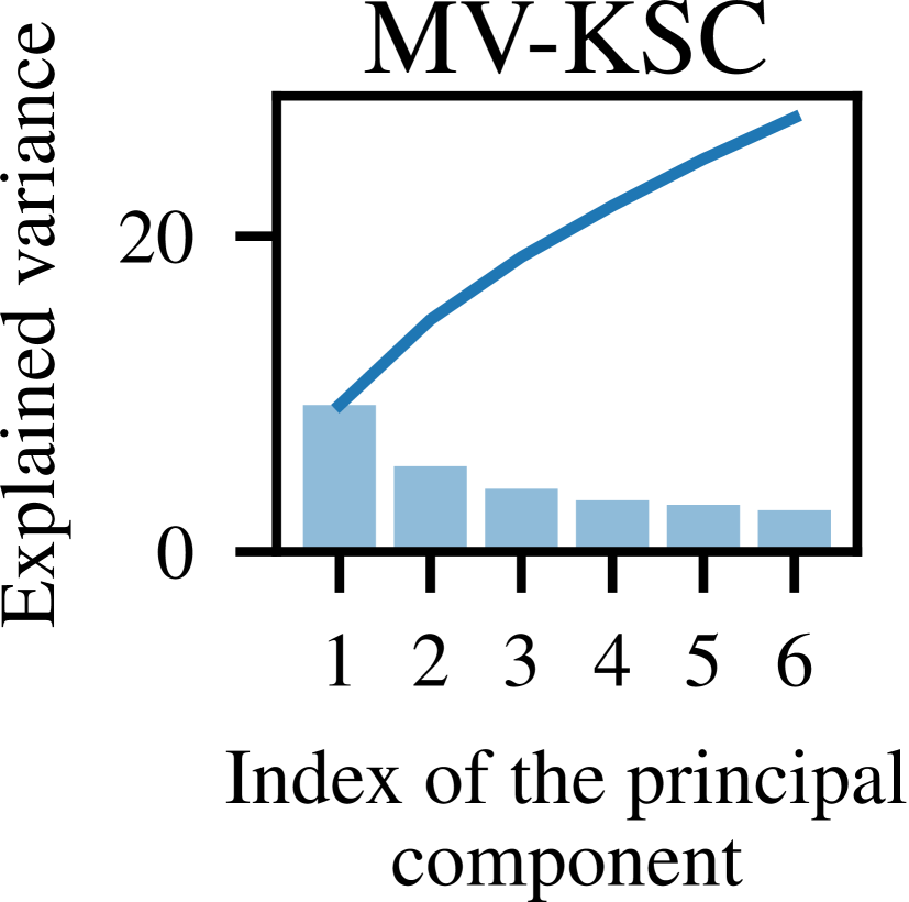
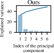
Figure 8: Explained variance for Ads ($k=2$). This plot also demonstrates our advantages in terms of a sharper eigenvalue decay compared to both the single-view based KSC and the multi-view based MvKSC.

4.3.2 Latent Space

With the common latent space, the latent variables, i.e., hidden features, in the constructed model can be directly visualized herein. Figure 9 plots the histogram of the latent variable distributions corresponding to Figure 7 on Synth 1. In Figure 9, the first and the second components are shown in the horizontal and perpendicular axis, respectively, where the color indicates the ground-truth cluster of each data point.

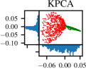
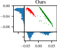
Figure 9: Scatter plot of the latent variable distribution for Synth 1. The histogram of $\bm{h}^{(1)}$ in KPCA gives an ungrouped distribution along the horizontal axis, while the two clusters are well separated in KSC and our method, and the Gaussian profiles in the histogram of our method are smoother and more distinctive.

Although KPCA and KSC both show a similar eigenvalue decay in Figure 7, the component computed by KSC can formulate better clustering, as shown in Figure 9. In KPCA, the first eigenvector shows clustering properties, but its histogram still shows a single ungrouped distribution rather than two distinct distributions for the clustering as in KSC. In our method, the two clusters in the latent space are well separated and their Gaussian profiles in the histogram are also smoother than KSC, indicating the more informative component in our method. This result demonstrates that the proposed common latent space is effective for multi-view learning in improving cluster separations, and might also facilitate future works, e.g., the generative model by sampling the distributions in the latent space. Further, the real-world dataset ImgC with $k=3$ clusters is evaluated in Figure 10, where two eigenvectors are needed for clustering, and thereby the histograms on both axes matter. Similar to Figure 9, our method shows better separations and more distinct histogram distributions for the clusters on both axes in the latent space. MvKSC works with a separate latent space for each view, each of which can have varied performances, which is inconvenient for a consistent analysis when dealing with many views. In contrast, our method determines a single latent space fusing all views in their dual representations to reveal the underlying clustering across views and meanwhile results in more separable clusters, boosting clustering performance and simplyifing pattern discovery.

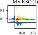
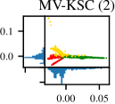
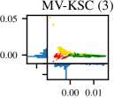
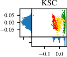
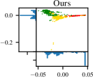
Figure 10: Scatter plot of the latent variable distribution for ImgC, where MvKSC works with separate latent spaces for each view. In KSC, the latent variable over the horizontal axis can separate the cluster in green (Aviation) from the those in yellow (Paintball) and red (Sports), but the other latent variable does not further identify Paintball and Sports. Both MvKSC and our method achieve better separations than KSC. Compared to MvKSC, especially on view 3, the clusters in our shared latent space are better separated and their Gaussian profiles in the histogram are more distinct.

4.3.3 Parameter sensitivity studies

In the proposed TMvKSCR, $\varrho$ and $\kappa^{[v]}$ can be tuned, as their incorporation enhances the couplings of views and integration of fusions. To better understand the roles of $\varrho$ and $\kappa$, studies are made for these two hyperparameters as follows. We firstly evaluate how $\varrho$, which combines the fusions as well as the tensor and matrix representations, affects the performance for multi-view clustering. In this experiment, all tested real-world datasets are used for evaluations, with other parameters fixed ($\kappa^{[v]}=1$ for $v=1,\dots,V$). Figure 11 presents the ARI results with varied $\varrho$. Then, we proceed to study the $\kappa^{[v]}$, where the Reuters dataset is exemplified for an illustration in Figure 12, which plots the surface of ARI with varying $\kappa^{[v]},v=1,2$ and fixing $\kappa^{[3]}=1$ and $\varrho=0.3$.

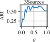
Figure 11: Study on the effects of $\varrho$ in the proposed method.

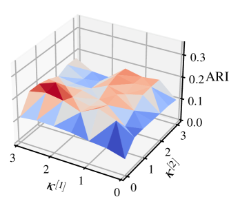
Figure 12: Study on the effects of $\kappa$ in the proposed method.

As shown in Figure 11, very low values of $\varrho$ lead to worse ARI on most datasets, suggesting that using tensors alone commonly does not result in good clustering. On the other hand, the optimal $\varrho$ for all datasets is greater than 0, showing the effectiveness of integrating tensor learning for high-order correlations. Hence, a good balance of $\varrho$ can improve the clustering performance. Especially for NUS, the tensor learning can bring significantly better ARI results, as smaller $\varrho$ gives higher ARI. $\varrho=0.25$ can be taken as a mild suggestion giving desirable performances for most cases. For the studies of $\kappa$ in Figure 12, simply setting $\kappa^{[1]}=\kappa^{[2]}=1$ already achieves good performance, while the optimal values of $\kappa^{[1]}$ and $\kappa^{[2]}$ are not necessarily exactly 1 and can be adjusted for enhanced performance, indicating that differently weighting the views can further boost the performance, which can be particularly meaningful with views varying significantly from each other. In this shown plot, a relatively higher value of $\kappa^{[1]}$ gives better performance.

5 Conclusion

In this paper, a novel method is proposed for multi-view spectral clustering under the framework of RKM. Firstly, we introduce a modified weighted conjugate feature duality to formulate a RKM for spectral clustering. Secondly, we propose to utilize shared hidden features with a common latent projection space, which realizes the couplings among different views and provides a simple alternative to perform interpretation and analysis. Thirdly, a tensor-based model is constructed to simultaneously incorporate feature maps of all views into tensors, which realizes high-order correlations and generalizes view fusions without increasing computational complexity in optimization. Fourthly, the resulting optimization simply needs to solve a single eigenvalue decomposition problem and the proposed shared latent space results in a computational complexity independent of number of views. Besides, the out-of-sample extension of our method enables to infer unseen data without re-training, which also greatly benefits the efficiency for large-scale cases. Numerical experiments on both synthetic and real-world datasets verify the effectiveness regarding clustering accuracy and efficiency of the proposed method. Through further analysis, we show that our method can capture more information in fewer components and that its shared latent space can boost informativeness in terms of data exploration and visualization. In future work, it would be of interest to investigate deep-level RKM and different tensor techniques for varied demands.

Appendix A More Experimental Details

The Synth 1 dataset consists of two-dimensional samples in three views $\{(\bm{x}_{i}^{[1]},\bm{x}_{i}^{[2]},\bm{x}_{i}^{[3]})\}_{i=1}^{1000}$ generated by a Gaussian mixture model. The cluster means for the first view are [1 1] and [3 4], for the second view are [1 2] and [2 2], and for the third view are [1 1] and [3 3]. The covariance matrices are $\bm{\Sigma}_{1}^{[1]}=\begin{bmatrix}1&0.5\\ 0.5&1.5\end{bmatrix}$, $\bm{\Sigma}_{2}^{[1]}=\begin{bmatrix}0.3&0.2\\ 0.2&0.6\end{bmatrix}$, $\bm{\Sigma}_{1}^{[2]}=\begin{bmatrix}1&-0.2\\ -0.2&1\end{bmatrix}$, $\bm{\Sigma}_{2}^{[2]}=\begin{bmatrix}0.6&0.1\\ 0.1&0.5\end{bmatrix}$, $\bm{\Sigma}_{1}^{[3]}=\begin{bmatrix}1.2&0.2\\ 0.2&1\end{bmatrix}$, $\bm{\Sigma}_{2}^{[3]}=\begin{bmatrix}1&0.4\\ 0.4&0.7\end{bmatrix}$. The Synth 2 dataset consists of two-dimensional samples in two views $\{(\bm{x}_{i}^{[1]},\bm{x}_{i}^{[2]})\}_{i=1}^{1000}$. For both views, data are allocated in an imbalanced way, i.e., 80% of the data points are located quite compactly in the dominant cluster while the remaining data are allocated more loosely in another cluster. More specifically, a point set $(\bm{x}^{[1]}_{i},\bm{x}^{[2]}_{i})$ is generated from a Gaussian mixture model. The cluster means for the first view are [1 1] and [2 2], and for the second view are [2 2] and [1 1]. The covariance matrices are $\bm{\Sigma}_{1}^{[1]}=\begin{bmatrix}0.1&0\\ 0&0.3\end{bmatrix}$, $\bm{\Sigma}_{2}^{[1]}=\begin{bmatrix}1.5&0.4\\ 0.4&1.2\end{bmatrix}$, $\bm{\Sigma}_{1}^{[2]}=\begin{bmatrix}0.3&0\\ 0&0.6\end{bmatrix}$, $\bm{\Sigma}_{2}^{[2]}=\begin{bmatrix}1&0.5\\ 0.5&0.9\end{bmatrix}$.

For high-dimensional real-world datasets in Table I, the 3Sources Text dataset consists of news articles from three online sources, corresponding to the three views: BBC, Reuters, and the Guardian [52]. Reuters [53] is from the L-Reuters Multilingual dataset [58], which contains documents of six categories written in five different languages. In Reuters, the English document is taken as the first view, while the corresponding French and German translation are the second view and third view, respectively. The Ads dataset contains images with hyperlink labeled as advertisement or not advertisement; the first view describes the image, the second view the URL and the last view the anchor URL [54, 55, 14]. The ImgC dataset consists of images of three sports: the first two views represent features of the image and the third view is the caption of the image [55]. The YT-VG dataset consists of videos of video games described in three views of text, image and audio features, as described in [56]. The NUS dataset contains images of ten classes described in five views using color histogram features, local self-similarity, pyramid HOG, SIFT, color SIFT and SURF features [57].

Regarding hyperparameter selection, we tune the hyperparameters of each tested method by grid search in the ranges suggested by the authors in their papers. In particular, one of the hyperparameters of COMIC, i.e., the clustering threshold $\varepsilon$, controls the estimated number of clusters $\hat{k}$. COMIC can normally overestimate the number of clusters $\hat{k}$ giving the worst performance among all the compared methods. If we keep the estimated number of clusters $\hat{k}$ to the real $k$, the performance is still inferior. Thus, we make a mild balance to give improved results, i.e., $\varepsilon$ is tuned between 0 and 1 with $\hat{k}/N\leq 0.1$. The shared hyperparameters in all methods are tuned under the same settings, e.g., the kernel parameters are tuned in the same range. The RBF kernel is used for the two synthetic datasets, Ads, NUS datasets, and the first two views of ImgC datasets. The 3Sources, Reuters, and the third view of ImgC datasets consist of high-dimensional text data, so we employ the normalized polynomial kernel of degree $d$. For the sparse and high-dimensional YT-VG dataset, we employ the linear kernel. The $\sigma^{2}$ of RBF kernels is tuned between $e^{-7}$ and $e^{7}$, the employed degree of the normalized polynomial kernel is $d\in\{1,2\}$, and the $t$ parameter is chosen between $e^{-5}$ and $e^{5}$. For MvKSC, the assignment can be done by both $\bm{e}^{[v]}$ and $\bm{e}_{\text{mean}}$, and we report their best results, while in our method TMvKSCR we use the assignment $\bm{e}_{\text{mean}}$ with $\varrho$ tuned between 0 and 1 and $\kappa^{[v]}$ between 0 and 3. For Co-Reg, the best results of the two schemes, i.e., the pairwise and the centroid couplings, are reported. For SFMC, we use the suggested anchor selection method and the anchor rate of 0.5 as in their paper. For MVSCBP, we tune the number of salient points $m$, the $r$ parameter and the number of nearest neighbors. The specific hyperparameters owned by individual methods are tuned separately as described above.

References

- [1] U. Von Luxburg, “A tutorial on spectral clustering,” Statistics and computing, vol. 17, no. 4, pp. 395–416, 2007.
- [2] F. R. Chung and F. C. Graham, Spectral graph theory. American Mathematical Society, 1997, no. 92.
- [3] J. Shi and J. Malik, “Normalized cuts and image segmentation,” IEEE Transactions on Pattern Analysis and Machine Intelligence, vol. 22, no. 8, pp. 888–905, 2000.
- [4] A. Y. Ng, M. I. Jordan, and Y. Weiss, “On spectral clustering: Analysis and an algorithm,” in Advances in Neural Information Processing Systems, 2002, pp. 849–856.
- [5] J. Ma, Y. Ma, and C. Li, “Infrared and visible image fusion methods and applications: A survey,” Information Fusion, vol. 45, pp. 153–178, 2019.
- [6] K. D. Yang, A. Belyaeva, S. Venkatachalapathy, K. Damodaran, A. Katcoff, A. Radhakrishnan, G. V. Shivashankar, and C. Uhler, “Multi-domain translation between single-cell imaging and sequencing data using autoencoders,” Nature Communications, vol. 12, no. 1, p. 31, Jan. 2021.
- [7] J. Zhao, X. Xie, X. Xu, and S. Sun, “Multi-view learning overview: Recent progress and new challenges,” Information Fusion, vol. 38, pp. 43–54, 2017.
- [8] G. Lin, H. Zhu, X. Kang, C. Fan, and E. Zhang, “Feature structure fusion and its application,” Information Fusion, vol. 20, pp. 146–154, 2014.
- [9] X. Xie and S. Sun, “Multi-view clustering ensembles,” in International Conference on Machine Learning and Cybernetics, vol. 1, 2013, pp. 51–56.
- [10] A. J. Bekker, M. Shalhon, H. Greenspan, and J. Goldberger, “Multi-view probabilistic classification of breast microcalcifications,” IEEE Transactions on Medical Imaging, vol. 35, no. 2, pp. 645–653, 2015.
- [11] J. Farquhar, D. Hardoon, H. Meng, J. S. Shawe-Taylor, and S. Szedmak, “Two view learning: SVM-2K, theory and practice,” in Advances in Neural Information Processing Systems, vol. 18, 2006, pp. 355–362.
- [12] A. Kumar, P. Rai, and H. Daume, “Co-regularized multi-view spectral clustering,” in Advances in Neural Information Processing Systems, vol. 24, 2011, pp. 1413–1421.
- [13] G. Andrew, R. Arora, J. Bilmes, and K. Livescu, “Deep canonical correlation analysis,” in International Conference on Machine Learning, 2013, pp. 1247–1255.
- [14] Y. Luo, D. Tao, K. Ramamohanarao, C. Xu, and Y. Wen, “Tensor canonical correlation analysis for multi-view dimension reduction,” IEEE Transactions on Knowledge and Data Engineering, vol. 27, pp. 3111–3124, 2015.
- [15] X. Peng, Z. Huang, J. Lv, H. Zhu, and J. T. Zhou, “COMIC: Multi-view clustering without parameter selection,” in International Conference on Machine Learning, 2019, pp. 5092–5101.
- [16] C. Zhang, H. Fu, S. Liu, G. Liu, and X. Cao, “Low-rank tensor constrained multiview subspace clustering,” in IEEE International Conference on Computer Vision, 2015, pp. 1582–1590.
- [17] L. Parsons, E. Haque, and H. Liu, “Subspace clustering for high dimensional data: a review,” ACM SIGKDD Explorations Newsletter, vol. 6, no. 1, pp. 90–105, 2004.
- [18] Y. Xie, D. Tao, W. Zhang, Y. Liu, L. Zhang, and Y. Qu, “On unifying multi-view self-representations for clustering by tensor multi-rank minimization,” International Journal of Computer Vision, vol. 126, no. 11, pp. 1157–1179, 2018.
- [19] G.-Y. Zhang, Y.-R. Zhou, C.-D. Wang, D. Huang, and X.-Y. He, “Joint representation learning for multi-view subspace clustering,” Expert Systems with Applications, vol. 166, p. 113913, 2021.
- [20] J. Lv, Z. Kang, B. Wang, L. Ji, and Z. Xu, “Multi-view subspace clustering via partition fusion,” Information Sciences, vol. 560, pp. 410–423, 2021.
- [21] C. Alzate and J. A. K. Suykens, “Multiway spectral clustering with out-of-sample extensions through weighted kernel PCA,” IEEE Transactions on Pattern Analysis and Machine Intelligence, vol. 32, no. 2, pp. 335–347, 2010.
- [22] R. Xia, Y. Pan, L. Du, and J. Yin, “Robust multi-view spectral clustering via low-rank and sparse decomposition,” in Proceedings of the AAAI Conference on Artificial Intelligence, vol. 28, no. 1, 2014.
- [23] D. Zhou and C. J. Burges, “Spectral clustering and transductive learning with multiple views,” in the International Conference on Machine learning, 2007, pp. 1159–1166.
- [24] F. Nie, G. Cai, J. Li, and X. Li, “Auto-weighted multi-view learning for image clustering and semi-supervised classification,” IEEE Transactions on Image Processing, vol. 27, no. 3, pp. 1501–1511, 2017.
- [25] K. Zhan, C. Zhang, J. Guan, and J. Wang, “Graph learning for multiview clustering,” IEEE Transactions on Cybernetics, vol. 48, no. 10, pp. 2887–2895, 2018.
- [26] K. Zhan, F. Nie, J. Wang, and Y. Yang, “Multiview consensus graph clustering,” IEEE Transactions on Image Processing, vol. 28, no. 3, pp. 1261–1270, 2018.
- [27] X. Li, H. Zhang, R. Wang, and F. Nie, “Multiview clustering: A scalable and parameter-free bipartite graph fusion method,” IEEE Transactions on Pattern Analysis and Machine Intelligence, vol. 44, no. 1, pp. 330–344, 2022.
- [28] Y. Li, F. Nie, H. Huang, and J. Huang, “Large-scale multi-view spectral clustering via bipartite graph,” in Proceedings of the AAAI Conference on Artificial Intelligence, 2015.
- [29] J. A. K. Suykens, T. Van Gestel, J. De Brabanter, B. De Moor, and J. P. Vandewalle, Least Squares Support Vector Machines. World scientific, 2002.
- [30] L. Houthuys, R. Langone, and J. A. K. Suykens, “Multi-view kernel spectral clustering,” Information Fusion, vol. 44, pp. 46–56, 2018.
- [31] J. A. K. Suykens, “Deep restricted kernel machines using conjugate feature duality,” Neural Computation, vol. 29, no. 8, pp. 2123–2163, 2017.
- [32] G. E. Hinton, S. Osindero, and Y.-W. Teh, “A fast learning algorithm for deep belief nets,” Neural Computation, vol. 18, no. 7, pp. 1527–1554, 2006.
- [33] F. Tonin, P. Patrinos, and J. A. Suykens, “Unsupervised learning of disentangled representations in deep restricted kernel machines with orthogonality constraints,” Neural Networks, vol. 142, pp. 661–679, 2021.
- [34] F. Tonin, A. Pandey, P. Patrinos, and J. A. K. Suykens, “Unsupervised energy-based out-of-distribution detection using Stiefel-restricted kernel machine,” in International Joint Conference on Neural Networks, 2021.
- [35] A. Pandey, J. Schreurs, and J. A. K. Suykens, “Generative restricted kernel machines: A framework for multi-view generation and disentangled feature learning,” Neural Networks, vol. 135, pp. 177–191, 2021.
- [36] A. Pandey, M. Fanuel, J. Schreurs, and J. A. K. Suykens, “Disentangled representation learning and generation with manifold optimization,” Neural Computation, 2022.
- [37] L. Houthuys and J. A. K. Suykens, “Tensor-based restricted kernel machines for multi-view classification,” Information Fusion, vol. 68, pp. 54–66, 2021.
- [38] X. Cai, F. Nie, H. Huang, and F. Kamangar, “Heterogeneous image feature integration via multi-modal spectral clustering,” in CVPR 2011, Jun. 2011, pp. 1977–1984.
- [39] S. Wang, X. Liu, E. Zhu, C. Tang, J. Liu, J. Hu, J. Xia, and J. Yin, “Multi-view clustering via late fusion alignment maximization.” in Proceedings of the International Joint Conference on Artificial Intelligence, 2019, pp. 3778–3784.
- [40] X. Liu, L. Liu, Q. Liao, S. Wang, Y. Zhang, W. Tu, C. Tang, J. Liu, and E. Zhu, “One pass late fusion multi-view clustering,” in Proceedings of the International Conference on Machine Learning, 2021, pp. 6850–6859.
- [41] J. Liu, X. Liu, Y. Yang, L. Liu, S. Wang, W. Liang, and J. Shi, “One-pass multi-view clustering for large-scale data,” in Proceedings of the IEEE/CVF International Conference on Computer Vision, 2021, pp. 12 344–12 353.
- [42] M. Meilă and J. Shi, “A random walks view of spectral segmentation,” in International Workshop on Artificial Intelligence and Statistics, vol. R3, 2001, pp. 203–208.
- [43] J. Ham, D. D. Lee, S. Mika, and B. Schölkopf, “A kernel view of the dimensionality reduction of manifolds,” in the International Conference on Machine learning, 2004, p. 47.
- [44] R. T. Rockafellar, Conjugate duality and optimization. SIAM, 1974.
- [45] V. N. Vapnik, “An overview of statistical learning theory,” IEEE Transactions on Neural Networks, vol. 10, no. 5, pp. 988–999, 1999.
- [46] A. Pandey, J. Schreurs, and J. A. K. Suykens, “Robust generative restricted kernel machines using weighted conjugate feature duality,” in International Conference on Machine Learning, Optimization, and Data Science. Springer, 2020, pp. 613–624.
- [47] J. Mercer, “Functions of positive and negative type, and their connection with the theory of integral equations,” Philosophical Transactions of the Royal Society A, vol. 209, no. 441-458, pp. 415–446, 1909.
- [48] T. G. Dietterich and G. Bakiri, “Solving multiclass learning problems via error-correcting output codes,” Journal of Artificial Intelligence Research, vol. 2, pp. 263–286, 1994.
- [49] C. Alzate and J. A. K. Suykens, “Out-of-sample eigenvectors in kernel spectral clustering,” in International Joint Conference on Neural Networks, 2011, pp. 2349–2356.
- [50] R. Mall, R. Langone, and J. A. K. Suykens, “Kernel spectral clustering for big data networks,” Entropy, vol. 15, no. 5, pp. 1567–1586, 2013.
- [51] L. Houthuys, R. Langone, and J. A. K. Suykens, “Multi-view least squares support vector machines classification,” Neurocomputing, vol. 282, pp. 78–88, 2018.
- [52] D. Greene and P. Cunningham, “A matrix factorization approach for integrating multiple data views,” in Joint European Conference on Machine Learning and Knowledge Discovery in Databases, 2009, pp. 423–438.
- [53] J. Liu, C. Wang, J. Gao, and J. Han, “Multi-view clustering via joint nonnegative matrix factorization,” in Proceedings of SIAM International Conference on Data Mining, 2013, pp. 252–260.
- [54] N. Kushmerick, “Learning to remove internet advertisements,” in Annual Conference on Autonomous Agents, 1999, p. 175–181.
- [55] T. Kolenda, L. K. Hansen, J. Larsen, and O. Winther, “Independent component analysis for understanding multimedia content,” in IEEE Workshop on Neural Networks for Signal Processing, 2002, pp. 757–766.
- [56] O. Madani, M. Georg, and D. A. Ross, “On using nearly-independent feature families for high precision and confidence,” in Proceedings of the Asian Conference on Machine Learning, vol. 25, 2012, pp. 269–284.
- [57] T.-S. Chua, J. Tang, R. Hong, H. Li, Z. Luo, and Y. Zheng, “NUS-WIDE: a real-world web image database from National University of Singapore,” in International Conference on Image and Video Retrieval, vol. 34, 2009, pp. 1–9.
- [58] D. Dua and C. Graff, “UCI machine learning repository,” 2017. [Online]. Available: http://archive.ics.uci.edu/ml
- [59] L. Hubert and P. Arabie, “Comparing partitions,” Journal of Classification, vol. 2, no. 1, pp. 193–218, 1985.
- [60] A. Strehl and J. Ghosh, “Cluster ensembles - a knowledge reuse framework for combining multiple partitions,” Journal of Machine Learning Research, vol. 3, pp. 583–617, 2002.
- [61] S. Romano, N. X. Vinh, J. Bailey, and K. Verspoor, “Adjusting for chance clustering comparison measures,” Journal of Machine Learning Research, vol. 17, no. 1, pp. 4635–4666, 2016.
- [62] A. Amelio and C. Pizzuti, “Correction for closeness: Adjusting normalized mutual information measure for clustering comparison,” Computational Intelligence, vol. 33, no. 3, pp. 579–601, 2017.
- [63] M. Girolami, “Orthogonal series density estimation and the kernel eigenvalue problem,” Neural Computation, vol. 14, no. 3, pp. 669–688, 2002.