Change Point Detection for High-dimensional Linear Models: A General Tail-adaptive Approach

Abstract

We study the change point detection problem for high-dimensional linear regression models. The existing literature mainly focused on the change point estimation with stringent sub-Gaussian assumptions on the errors. In practice, however, there is no prior knowledge about the existence of a change point or the tail structures of errors. To address these issues, in this paper, we propose a novel tail-adaptive approach for simultaneous change point testing and estimation. The method is built on a new loss function which is a weighted combination between the composite quantile and least squared losses, allowing us to borrow information of the possible change points from both the conditional mean and quantiles. For the change point testing, based on the adjusted $L_{2}$-norm aggregation of a weighted score CUSUM process, we propose a family of individual testing statistics with different weights to account for the unknown tail structures. Combining the individual tests, a tail-adaptive test is further constructed that is powerful for sparse alternatives of regression coefficients’ changes under various tail structures. For the change point estimation, a family of argmax-based individual estimators is proposed once a change point is detected. In theory, for both individual and tail-adaptive tests, the bootstrap procedures are proposed to approximate their limiting null distributions. Under some mild conditions, we justify the validity of the new tests in terms of size and power under the high-dimensional setup. The corresponding change point estimators are shown to be rate optimal up to a logarithm factor. Moreover, combined with the wild binary segmentation technique, a new algorithm is proposed to detect multiple change points in a tail-adaptive manner. Extensive numerical results are conducted to illustrate the appealing performance of the proposed method.

Keywords: Efficient computation, Heavy tail, High dimensions, Structure change

1 Introduction

With the advances of data collection and storage capacity, large scale/high-dimensional data are ubiquitous in many scientific fields ranging from genomics, finance, to social science. Due to the complex data generation mechanism, the heterogeneity, also known as the structural break, has become a common phenomenon for high-dimensional data, where the underlying model of data generation changes and the identically distributed assumption may not hold anymore. Change point analysis is a powerful tool for handling structural changes since the seminal work by Page (1955). It received considerable attentions in recent years and has a lot of real applications in various fields including genomics (Liu et al., 2020), social science (Roy et al., 2017), financial contagion (Pesaran and Pick, 2007) in economy, and even for the recent COVID-19 pandemic studies (Jiang et al., 2021). Motivated by this, in this paper, we study the change point testing and estimation problem in the high-dimensional linear regression setting.

Specifically, we are interested in the following model and detect possible change points:

$$Y=\bm{X}^{\top}\bm{\beta}+\epsilon,\vspace{-0.2cm}$$

where $Y\in\mathbb{R}$ is the response variable, $\bm{X}=(X_{1},\ldots,X_{p})\in\mathbb{R}^{p}$ is the covariate vector, $\bm{\beta}=(\beta_{1},\ldots,\beta_{p})^{\top}$ is a $p\times 1$ unknown vector of coefficients, and $\epsilon\in\mathbb{R}$ is the error term. Suppose we have $n$ independent but (time) ordered realizations $\{(Y_{i},\bm{X}_{i}),i=1,\ldots,n\}$ with $\bm{X}_{i}=(X_{i1},\ldots,X_{ip})^{\top}$. For each time point $i$, consider the following regression model:

$$Y_{i}=\bm{X}_{i}^{\top}\bm{\beta}_{i}+\epsilon_{i},\vspace{-0.2in}$$ (1.1)

where $\bm{\beta}_{i}=(\beta_{i1},\ldots,\beta_{ip})^{\top}$ is the regression coefficient vector for the $i$-th observation, and $\epsilon_{i}$ is the error term. For the above model, our first question is whether there is a change point. This can be formulated as the following hypothesis testing problem:

$$\small\begin{array}[]{ll}\mathbf{H}_{0}:\bm{\beta}_{1}=\bm{\beta}_{2}=\cdots=\bm{\beta}_{n}\leavevmode\nobreak\ \leavevmode\nobreak\ \text{v.s.}\leavevmode\nobreak\ \leavevmode\nobreak\ \mathbf{H}_{1}:\bm{\beta}^{(1)}=\bm{\beta}_{1}=\cdots=\bm{\beta}_{k_{1}}\neq\bm{\beta}_{k_{1}+1}=\cdots=\bm{\beta}_{n}:=\bm{\beta}^{(2)},\end{array}\vspace{-0.2in}$$ (1.2)

where $k_{1}$ is the possible but unknown change point location. In this article, we assume $k_{1}=\lfloor nt_{1}\rfloor$ with $0<t_{1}<1$. According to (1.2), the linear regression structure between $Y$ and $\bm{X}$ remains homogeneous if $\mathbf{H}_{0}$ holds, and otherwise there is a change point $k_{1}$ that divides the data into two segments with different regression coefficients $\bm{\beta}^{(1)}$ and $\bm{\beta}^{(2)}$. Our second goal of this paper is to identify the change point location if we reject $\mathbf{H}_{0}$ in (1.2). Note that the above two goals are referred as change point testing and estimation, respectively. In the practical use, both testing and estimation are important since practitioners typically have no prior knowledge about either the existence of a change point or its location. Therefore, it is very useful to consider simultaneous change point detection and estimation. Furthermore, the tail structure of the error $\epsilon_{i}$ in Model (1.1) is typically unknown, which could significantly affect the performance of the change point detection and estimation. In the existing literature, the performance guarantee of most methods on change point estimation relies on the assumption that the error $\epsilon_{i}$ follows a Gaussian/sub-Gaussian distribution. Such an assumption could be violated in practice when the data distribution is heavy-tailed or contaminated by outliers. While some robust methods can address these issues, they may lose efficiency when errors are indeed sub-Gaussian distributed. It is also very difficult to estimate the tail structures and construct a corresponding change point method based on that. Hence, it is of great interest to construct a tail-adaptive change point detection and estimation method for high-dimensional linear models.

1.1 Contribution

Motivated by our previous discussion, in this paper, under the high-dimensional setup with $p\gg n$, we propose a tail-adaptive procedure for simultaneous change point testing and estimation in linear regression models. The proposed method relies on a new loss function in our change point estimation procedure, which is a weighted combination between the composite quantile loss proposed in Zou and Yuan (2008) and the least squared loss with the weight $\alpha\in[0,1]$ for balancing the efficiency and robustness. Thanks to this new loss function with different $\alpha$, we are able to borrow information related to the possible change point from both the conditional mean and quantiles in Model (1.1). Therefore, besides controlling the type I error to any desirable level when $\mathbf{H}_{0}$ holds, the proposed method simultaneously enjoys high power and accuracy for change point testing and identification across various underlying error distributions including both lighted and heavy-tailed errors when there exists a change point. By combining our single change point estimation method with the wild binary segmentation (WBS) technique (Fryzlewicz, 2014), we also generalize our method for detecting multiple change points in Model (1.1).

In terms of our theoretical contribution, for each given $\alpha$, a novel score-based $\mathbb{R}^{p}$-dimensional individual CUSUM process $\{{\bm{C}}_{\alpha}(t),t\in[0,1]\}$ is proposed. Based on this, we construct a family of individual-based testing statistics $\{T_{\alpha},\alpha\in[0,1]\}$ via aggregating $\bm{C}_{\alpha}(t)$ using the $\ell_{2}$-norm of its first $s_{0}$ largest order statistics, known as the $(s_{0},2)$-norm proposed in Zhou et al. (2018). A high-dimensional bootstrap procedure is introduced to approximate $T_{\alpha}$’s limiting null distributions (See Algorithm 1). The proposed bootstrap method only requires mild conditions on the covariance structures of $\bm{X}$ and the underlying error distribution $\epsilon$, and is free of tuning parameters and computationally efficient. Furthermore, combining the corresponding individual tests in $\{T_{\alpha},\alpha\in[0,1]\}$, we construct a tail-adaptive test statistic $T_{\rm ad}$ by taking the minimum $P$-values of $\{T_{\alpha},\alpha\in[0,1]\}$. The proposed tail-adaptive method $T_{\rm ad}$ chooses the best individual test according to the data and thus enjoys simultaneous high power across various tail structures. Theoretically, we adopt a low-cost bootstrap method for approximating the limiting distribution of $T_{\rm ad}$. In terms of size and power, for both individual and tail-adaptive tests, we prove that the corresponding test can control the type I error for any given significance level if $\mathbf{H}_{0}$ holds, and reject the null hypothesis with probability tending to one otherwise.

As for the change point estimation, once $\mathbf{H}_{0}$ is rejected by our test, based on each individual test statistic, we can estimate its location via taking argmax with respect to different candidate locations $t\in(0,1)$ for the $(s_{0},2)$-norm aggregated process $\{\|\bm{C}_{\alpha}(t)\|_{(s_{0},2)},t\in[0,1]\}$. Under some regular conditions, for each individual based estimator $\{\widehat{t}_{\alpha},\alpha\in[0,1]\}$, we can show that the estimation error is rate optimal up to a $\log(pn)$ factor. Hence, the proposed individual estimators for the change point location allow the signal jump size scale well with $(n,p)$ and are consistent as long as $SNR(\alpha,\bm{\tau})\|\bm{\Sigma}(\bm{\beta}^{(2)}-\bm{\beta}^{(1)})\|_{(s_{0},2)}\gg\sqrt{\log(pn)/n}$ holds, where $SNR(\alpha,\bm{\tau})$ is the signal to noise constant related to the loss function and the underlying error distribution. It is worth noting that the computational cost for obtaining $\{\widehat{t}_{\alpha},\alpha\in[0,1]\}$ is only $O(\rm Lasso(n,p))$ operations, where $\rm Lasso(n,p)$ is the cost to compute the Lasso estimator for the corresponding weighted loss. This can be much more efficient than the existing works with $O(\rm nLasso(n,p))$ operations in Lee et al. (2016, 2018) and $O(\rm 2Lasso(n,p))$ operations in Kaul et al. (2019).

1.2 Related literature

For the low dimensional setting with a fixed $p$ and $p<n$, change point analysis for linear regression models has been well-studied. Specifically, Quandt (1958) considered testing (1.2) for a simple regression model with $p=2$. Other extensions include the maximum likelihood ratio tests (Horváth, 1995), partial sums of regression residuals (Gombay and Horváth, 1994; Bai and Perron, 1998), and the union intersection test (Horváth and Shao, 1995). Other related methods include Qu (2008); Zhang et al. (2014); Oka and Qu (2011); Lee et al. (2011) and among others.

Due to the curse of dimensionality, on the other hand, only a few papers studied high-dimensional change point analysis, which mainly focused on the change point estimation. See Lee et al. (2016); Kaul et al. (2019); Lee et al. (2018); Leonardi and Bühlmann (2016); Zhang et al. (2015); Wang et al. (2021, 2022). However, none of the aforementioned papers develop hypothesis testing procedure, which is the prerequisite for the change point detection. Furthermore, most existing literature requires strong conditions on the underlying errors $\epsilon_{i}$ for deriving the desirable theoretical properties, which may not be applicable when the data are heavy-tailed or contaminated by outliers. One possible solution is to use the robust method such as median regression in Lee et al. (2018) for change point estimation. As discussed in Zou and Yuan (2008); Bradic et al. (2011); Zhao et al. (2014), when making statistical inference for homogeneous linear models, the asymptotic relative efficiency of median regression-based estimators compared to least squared-based is only about 64% in both low and high dimensions. In addition, inference based on quantile regression can have arbitrarily small relative efficiency compared to the least squared based regression. Our proposed tail-adaptive method is the first one that can perform simultaneous change point testing and estimation for high-dimensional linear regression models with different distributions. In addition to controlling the type I error to any desirable level, the proposed method enjoys simultaneously high power and accuracy for the change point testing and identification across various underlying error distributions when there exists a change point. Besides literature in the regression setting, change point analysis has also been carried out for the setting of high-dimensional mean vectors and some mean vector-based extensions. See Aue et al. (2009); Jirak (2015); Cho et al. (2016); Liu et al. (2020)) and many others.

The rest of this paper is organized as follows. In Section 2, we introduce our new tail-adaptive methodology for detecting a single change point as well as multiple change points. In Section 3, we derive the theoretical results in terms of size and power as well as the change point estimation. In Section 4, we present our extensive simulation results. A real application to the S$\&$P 100 dataset is shown in Section 5. The concluding remarks are provided in Section 6. Detailed proofs and the full numerical results are given in the online supplementary materials.

Notations: We end this section by introducing some notations. For $\bm{v}=(v_{1},\ldots,v_{p})^{\top}\in\mathbb{R}^{p}$, we define its $\ell_{p}$ norm as $\|\bm{v}\|_{p}=(\sum_{j=1}^{d}|v_{j}|^{p})^{1/p}$ for $1\leq p\leq\infty$. For $p=\infty$, define $\|\bm{v}\|_{\infty}=\max_{1\leq j\leq d}|v_{j}|$. For any set ${\mathcal{S}}$, denote its cardinality by $|{\mathcal{S}}|$. For two real numbered sequences $a_{n}$ and $b_{n}$, we set $a_{n}=O(b_{n})$ if there exits a constant $C$ such that $|a_{n}|\leq C|b_{n}|$ for a sufficiently large $n$; $a_{n}=o(b_{n})$ if $a_{n}/b_{n}\rightarrow 0$ as $n\rightarrow\infty$; $a_{n}\asymp b_{n}$ if there exists constants $c$ and $C$ such that $c|b_{n}|\leq|a_{n}|\leq C|b_{n}|$ for a sufficiently large $n$. For a sequence of random variables (r.v.s) $\{\xi_{1},\xi_{2},\ldots\}$, we set $\xi_{n}\xrightarrow{{\mathbb{P}}}\xi$ if $\xi_{n}$ converges to $\xi$ in probability as $n\rightarrow\infty$. We also denote $\xi_{n}=o_{p}(1)$ if $\xi_{n}\xrightarrow{{\mathbb{P}}}0$. For a $n\times p$ matrix $\mathbf{X}$, denote $\mathbf{X}_{i}$ and $\mathbf{X}^{j}$ as its $i$-th row and $j$-th column respectively. We define $\lfloor x\rfloor$ as the largest integer less than or equal to $x$ for $x\geq 0$. Denote $(\mathcal{X},\mathcal{Y})=\{(\bm{X}_{1},Y_{1}),\ldots,(\bm{X}_{n},Y_{n})\}$.

2 Methodology

In Section 2.1, we construct a family of oracle individual testing statistics $\{\widetilde{T}_{\alpha},\alpha\in[0,1]\}$ for single change point detection. To estimate the unknown variance in $\widetilde{T}_{\alpha}$, in Section 2.2, a weighted variance estimation that is consistent under both $\mathbf{H}_{0}$ and $\mathbf{H}_{1}$ is proposed. With the estimated variance, a family of data-driven testing statistics $\{{T}_{\alpha},\alpha\in[0,1]\}$ is proposed for change point detection. To approximate the limiting null distribution of ${T}_{\alpha}$, we introduce a novel bootstrap procedure in Section 2.3. In practice, the tail structure of the error term is typically unknown. Hence, it is desirable to combine the individual testing statistics $\{{T}_{\alpha},\alpha\in[0,1]\}$ for yielding a powerful tail-adaptive method. To solve this problem, in Section 2.4, a tail-adaptive testing statistic $T_{\rm ad}$ is proposed. Lastly, we combine our testing procedure with the WBS technique for detecting multiple change points.

2.1 Single change point detection

In this section, we introduce our new methodology for Problem (1.2). We first focus on detecting a single change point in Model (1.1). In this case, Model (1.1) reduces to:

$$Y_{i}=\bm{X}_{i}^{\top}\bm{\beta}^{(1)}\mathbf{1}\{i\leq k_{1}\}+\bm{X}_{i}^{\top}\bm{\beta}^{(2)}\mathbf{1}\{i>k_{1}\}+\epsilon_{i},\leavevmode\nobreak\ \text{for}\leavevmode\nobreak\ i=1,\ldots,n.\vspace{-0.2in}$$ (2.1)

In this paper, we assume $k_{1}=\lfloor nt_{1}\rfloor$ for some constant $t_{1}\in(0,1)$. Note that $t_{1}$ is called the relative change point location. We assume the change point does not occur at the begining or end of data observations. Specifically, suppose there exists a constant $q_{0}\in(0,0.5)$ such that $q_{0}\leq t_{1}\leq 1-q_{0}$ holds, which is a common assumption in the literature (e.g., Dette et al., 2018; Jirak, 2015). For Model (2.1), given $\bm{X}_{i}$, the conditional mean of $Y_{i}$ becomes:

$${\mathbb{E}}[Y_{i}\,|\,\bm{X}_{i}]=\bm{X}_{i}^{\top}\bm{\beta}^{(1)}\mathbf{1}\{i\leq k_{1}\}+\bm{X}_{i}^{\top}\bm{\beta}^{(2)}\mathbf{1}\{i>k_{1}\}.\vspace{-0.2in}$$ (2.2)

Moreover, let $0<\tau_{1}<\ldots<\tau_{K}<1$ be $K$ candidate quantile indices. For each $\tau_{k}\in(0,1)$, let $b_{k}^{(0)}:=\inf\{t:{\mathbb{P}}(\epsilon\leq t)\geq\tau_{k}\}$ be the $\tau_{k}$-th theoretical quantile for the generic error term $\epsilon$ in Model (2.1). Then, conditional on $\bm{X}_{i}$, the $\tau_{k}$-th quantile for $Y_{i}$ becomes:

$$Q_{\tau_{k}}(Y_{i}|\bm{X}_{i})=b_{k}^{(0)}+\bm{X}_{i}^{\top}\bm{\beta}^{(1)}\mathbf{1}\{i\leq k_{1}\}+\bm{X}_{i}^{\top}\bm{\beta}^{(2)}\mathbf{1}\{i>k_{1}\},\leavevmode\nobreak\ k=1,\ldots,K,\vspace{-0.2in}$$ (2.3)

where $Q_{\tau_{k}}(Y_{i}|\bm{X}_{i}):=\inf\{t:{\mathbb{P}}(Y_{i}\leq t|\bm{X}_{i})\geq\tau_{k}\}$. Hence, if there exists a change point in Model (2.1), both the conditional mean and the conditional quantile change after the change point. This suggests that we can make change point inference for $\bm{\beta}^{(1)}$ and $\bm{\beta}^{(2)}$ using either (2.2) or (2.3). To propose our new testing statistic, we first introduce the following weighted composite loss function. In particular, let $\alpha\in[0,1]$ be some candidate weight. Define the weighted composite loss function as:

$$\ell_{\alpha}(\bm{x},y;\widetilde{\bm{\tau}},\bm{b},\bm{\beta}):=(1-\alpha)\dfrac{1}{K}\sum_{k=1}^{K}\rho_{\tau_{k}}(y-b_{k}-\bm{x}^{\top}\bm{\beta})+\dfrac{\alpha}{2}(y-\bm{x}^{\top}\bm{\beta})^{2},\vspace*{-0.2in}$$ (2.4)

where $\rho_{\tau}(t):=t(\tau-\mathbf{1}\{t\leq 0\})$ is the check loss function (Koenker and Bassett Jr, 1978), $\widetilde{\bm{\tau}}:=(\tau_{1},\ldots,\tau_{K})^{\top}$ are user-specified $K$ quantile levels, and $\bm{b}=(b_{1},\ldots,b_{K})^{\top}\in\mathbb{R}^{K}$ and $\bm{\beta}=(\beta_{1},\ldots,\beta_{p})^{\top}\in\mathbb{R}^{p}$. Note that we can regard $\ell_{\alpha}(\bm{x},y;\widetilde{\bm{\tau}},\bm{b},\bm{\beta})$ as a weighted loss function between the composite quantile loss and the squared error loss. For example, for $\alpha=1$, it reduces to the ordinary least squared-based loss function with $\ell_{1}(\bm{x},y)=(y-\bm{x}^{\top}\bm{\beta})^{2}/2$. When $\alpha=0$, it is the composite quantile loss function $\ell_{0}(\bm{x},y)=\sum_{k=1}^{K}\rho_{\tau_{k}}(y-b_{k}-\bm{x}^{\top}\bm{\beta})/K$ proposed in Zou and Yuan (2008). It is known that the least squared loss-based method has the best statistical efficiency when errors follow Gaussian distributions and the composite quantile loss is more robust when the error distribution is heavy-tailed or contaminated by outliers. As discussed before, in practice, it is challenging to obtain the tail structure of the error distribution and construct a corresponding change point testing method based on the error structure. Hence, we propose a weighted loss function by borrowing the information related to the possible change point from both the conditional mean and quantiles. More importantly, we use the weight $\alpha$ to balance the efficiency and robustness.

Our new testing statistic is based on a novel high-dimensional weighted score-based CUSUM process of the weighted composite loss function. In particular, for the composite loss function $\ell_{\alpha}(\bm{x},y;\widetilde{\bm{\tau}},\bm{b},\bm{\beta})$, define its score (subgradient) function ${\partial\ell_{\alpha}(\bm{x},y;\widetilde{\bm{\tau}},\bm{b},\bm{\beta})}/{\partial\bm{\beta}}$ with respect to $\bm{\beta}$ as:

$$\begin{array}[]{ll}\bm{Z}_{\alpha}(\bm{x},y;\widetilde{\bm{\tau}},\bm{b},\bm{\beta}):=\Big{[}\dfrac{1-\alpha}{K}\sum\limits_{k=1}^{K}\bm{x}\big{(}\mathbf{1}\{y-b_{k}-\bm{x}^{\top}\bm{\beta}\leq 0\}-\tau_{k}\big{)}\Big{]}-\alpha\big{[}\bm{x}(y-\bm{x}^{\top}\bm{\beta})\big{]}.\end{array}\vspace{-0.2in}$$ (2.5)

Using $\bm{Z}_{\alpha}(\bm{x},y;\widetilde{\bm{\tau}},\bm{b},\bm{\beta})$, for each $\alpha\in[0,1]$ and $t\in(0,1)$, we first define the oracle score-based CUSUM as follows:

$$\widetilde{\bm{C}}_{\alpha}(t;\widetilde{\bm{\tau}},\bm{b},\bm{\beta})=\dfrac{1}{\sqrt{n}\sigma(\alpha,\widetilde{\bm{\tau}})}\big{(}\sum\limits_{i=1}^{\lfloor nt\rfloor}\bm{Z}_{\alpha}(\bm{X}_{i},Y_{i};\widetilde{\bm{\tau}},\bm{b},\bm{\beta})-\dfrac{\lfloor nt\rfloor}{n}\sum\limits_{i=1}^{n}\bm{Z}_{\alpha}(\bm{X}_{i},Y_{i};\widetilde{\bm{\tau}},\bm{b},\bm{\beta})\big{)},\vspace{-0.2in}$$ (2.6)

where $\sigma^{2}(\alpha,\widetilde{\bm{\tau}}):=\text{Var}[(1-\alpha)e_{i}(\widetilde{\bm{\tau}})-\alpha\epsilon_{i})]$ with $e_{i}(\widetilde{\bm{\tau}}):=K^{-1}\sum\limits_{k=1}^{K}(\mathbf{1}\{\epsilon_{i}\leq b_{k}^{(0)}\}-\tau_{k})$. Note that we call $\widetilde{\bm{C}}_{\alpha}(t;\widetilde{\bm{\tau}},\bm{b},\bm{\beta})$ oracle since we assume $\sigma^{2}(\alpha,\widetilde{\bm{\tau}})$ is known. In Section 2.2, we will give the explicit form of $\sigma^{2}(\alpha,\widetilde{\bm{\tau}})$ under various combinations of $\alpha$ and $\widetilde{\bm{\tau}}$ and introduce its consistent estimator under both $\mathbf{H}_{0}$ and $\mathbf{H}_{1}$. In the following, to motivate our test statistics, we study the behaviors of $\widetilde{\bm{C}}_{\alpha}(t;\widetilde{\bm{\tau}},\bm{b},\bm{\beta})$ under $\mathbf{H}_{0}$ and $\mathbf{H}_{1}$ respectively. First, under $\mathbf{H}_{0}$, if we replace $\bm{\beta}=\bm{\beta}^{(0)}$ and $\bm{b}=\bm{b}^{(0)}$ in (2.6), the score based CUSUM becomes

$$\begin{array}[]{ll}\widetilde{\bm{C}}_{\alpha}(t;\widetilde{\bm{\tau}},\bm{b}^{(0)},\bm{\beta}^{(0)})=\dfrac{1}{\sqrt{n}\sigma(\alpha,\widetilde{\bm{\tau}})}\Big{(}\sum\limits_{i=1}^{\lfloor nt\rfloor}\bm{Z}_{\alpha}(\bm{X}_{i},Y_{i};\widetilde{\bm{\tau}},\bm{b}^{(0)},\bm{\beta}^{(0)})-\dfrac{\lfloor nt\rfloor}{n}\sum\limits_{i=1}^{n}\bm{Z}_{\alpha}(\bm{X}_{i},Y_{i};\widetilde{\bm{\tau}},\bm{b}^{(0)},\bm{\beta}^{(0)})\Big{)}.\end{array}\vspace{-0.15in}$$

By noting that under $\mathbf{H}_{0}$, we have $Y_{i}=\bm{X}_{i}^{\top}\bm{\beta}^{(0)}+\epsilon_{i}$, the above CUSUM reduces to the following $\mathbb{R}^{p}$–dimensional random noise based CUSUM process:

$$\begin{array}[]{ll}\widetilde{\bm{C}}_{\alpha}(t;\widetilde{\bm{\tau}},\bm{b}^{(0)},\bm{\beta}^{(0)})\\ =\dfrac{1}{\sqrt{n}\sigma(\alpha,\widetilde{\bm{\tau}})}\Big{(}\sum\limits_{i=1}^{\lfloor nt\rfloor}\bm{X}_{i}((1-\alpha)e_{i}(\widetilde{\bm{\tau}})-\alpha\epsilon_{i})-\dfrac{\lfloor nt\rfloor}{n}\sum\limits_{i=1}^{n}\bm{X}_{i}((1-\alpha)e_{i}(\widetilde{\bm{\tau}})-\alpha\epsilon_{i})\Big{)},\\ \end{array}\vspace{-0.2in}$$ (2.7)

whose asymptotic distribution can be easily characterized. Since both $\bm{b}^{(0)}$ and $\bm{\beta}^{(0)}$ are unknown, we need some proper estimators that can approximate them well under $\mathbf{H}_{0}$. In this paper, for each $\alpha\in[0,1]$, we obtain the estimators by solving the following optimization problem with the $L_{1}$ penalty:

$$\small(\widehat{\bm{b}}_{\alpha},\widehat{\bm{\beta}}_{\alpha})=\mathop{\text{\rm arg\,min}}_{\bm{b}\in\mathbb{R}^{K},\atop\bm{\beta}\in\mathbb{R}^{p}}\Big{[}(1-\alpha)\dfrac{1}{n}\sum_{i=1}^{n}\dfrac{1}{K}\sum_{k=1}^{K}\rho_{\tau_{k}}(Y_{i}-b_{i}-\bm{X}_{i}^{\top}\bm{\beta})+\dfrac{\alpha}{2n}\sum_{i=1}^{n}(Y_{i}-\bm{X}_{i}^{\top}\bm{\beta})^{2}+\lambda_{\alpha}\big{\|}\bm{\beta}\big{\|}_{1}\Big{]},$$ (2.8)

where $\widehat{\bm{b}}_{\alpha}:=(\widehat{b}_{\alpha,1},\cdots,\widehat{b}_{\alpha,K})^{\top}$, $\widehat{\bm{\beta}}_{\alpha}:=(\widehat{\beta}_{\alpha,1},\ldots,\widehat{\beta}_{\alpha,p})^{\top}$, and $\lambda_{\alpha}$ is the non-negative tuning parameter controlling the overall sparsity of $\widehat{\bm{\beta}}_{\alpha}$. Note that the above estimators are obtained using all observations $\{(\bm{X}_{1},Y_{1}),\ldots,(\bm{X}_{n},Y_{n})\}$. After obtaining $(\widehat{\bm{b}}_{\alpha}^{\top},\widehat{\bm{\beta}}_{\alpha}^{\top})$, we plug them into the score function in (2.6) and obtain the final $\mathbb{R}^{p}$–dimensional oracle score based CUSUM statistic as follows:

$$\widetilde{\bm{C}}_{\alpha}(t;\widetilde{\bm{\tau}},\widehat{\bm{b}}_{\alpha},\widehat{\bm{\beta}}_{\alpha})=\big{(}\widetilde{C}_{\alpha,1}(t;\widetilde{\bm{\tau}},\widehat{\bm{b}}_{\alpha},\widehat{\bm{\beta}}_{\alpha}),\ldots,\widetilde{C}_{\alpha,p}(t;\widetilde{\bm{\tau}},\widehat{\bm{b}}_{\alpha},\widehat{\bm{\beta}}_{\alpha})\big{)}^{\top},\leavevmode\nobreak\ \leavevmode\nobreak\ t\in[q_{0},1-q_{0}].\vspace{-0.2in}$$ (2.9)

Using $(\widehat{\bm{b}}_{\alpha},\widehat{\bm{\beta}}_{\alpha})$, we can prove that under $\mathbf{H}_{0}$, for each $\alpha\in[0,1]$, (2.9) can approximate the random-noise based CUSUM process in (2.7) under some proper norm aggregations. Next, we investigate the behavior of (2.9) under $\mathbf{H}_{1}$. Observe that the score based CUSUM has the following decomposition:

$$\widetilde{\bm{C}}_{\alpha}(t;\widetilde{\bm{\tau}},\widehat{\bm{b}}_{\alpha},\widehat{\bm{\beta}}_{\alpha})=\underbrace{{\widetilde{\bm{C}}_{\alpha}(t;\widetilde{\bm{\tau}},\bm{b}^{(0)},\bm{\beta}^{(0)})}}_{\rm\bf Random\leavevmode\nobreak\ Noise}+\underbrace{{\bm{\delta}_{\alpha}(t)}}_{\rm\bf Signal\leavevmode\nobreak\ Jump}+\underbrace{{\bm{R}_{\alpha}(t;\widehat{\bm{b}}_{\alpha},\widehat{\bm{\beta}}_{\alpha})}}_{\rm\bf Random\leavevmode\nobreak\ Bias},\vspace{-0.2in}$$ (2.10)

where $\widetilde{\bm{C}}_{\alpha}(t;\widetilde{\bm{\tau}},\bm{b}^{(0)},\bm{\beta}^{(0)})$ is the random noise based CUSUM process defined in (2.7), $\bm{R}_{\alpha}(t;\widehat{\bm{b}}_{\alpha},\widehat{\bm{\beta}}_{\alpha})$ is some random bias which has a very complicated form but can be controlled properly under $\mathbf{H}_{1}$, and $\bm{\delta}_{\alpha}(t)$ is the signal jump function. More specifically, let

$$SNR(\alpha,\widetilde{\bm{\tau}}):=\dfrac{(1-\alpha)\big{(}\dfrac{1}{K}\sum\limits_{k=1}^{K}f_{\epsilon}(b_{k}^{(0)})\big{)}+\alpha}{\sigma(\alpha,\widetilde{\bm{\tau}})},\vspace{-0.in}$$ (2.11)

where $f_{\epsilon}(t)$ is the probability density function of $\epsilon$, and define the signal jump function

$$\bm{\Delta}(t;\bm{\beta}^{(1)},\bm{\beta}^{(2)}):=n^{-\frac{3}{2}}\times\left\{\begin{array}[]{ll}{\lfloor nt\rfloor(n-\lfloor nt_{1}\rfloor)}\bm{\Sigma}\big{(}\bm{\beta}^{(1)}-\bm{\beta}^{(2)}\big{)},\leavevmode\nobreak\ \text{if}\leavevmode\nobreak\ t\leq t_{1},\\ {\lfloor nt_{1}\rfloor(n-\lfloor nt\rfloor)}\bm{\Sigma}\big{(}\bm{\beta}^{(1)}-\bm{\beta}^{(2)}\big{)},\leavevmode\nobreak\ \text{if}\leavevmode\nobreak\ t>t_{1}.\end{array}\right.\vspace{-0.2in}$$ (2.12)

Then, the signal jump $\bm{\delta}_{\alpha}(t)$ can be explicitly represented as the products of $SNR(\alpha,\widetilde{\bm{\tau}})$ and $\bm{\Delta}(t;\bm{\beta}^{(1)},\bm{\beta}^{(2)})$, which has the following explicit form:

$$\bm{\delta}_{\alpha}(t):=SNR(\alpha,\widetilde{\bm{\tau}})\times\bm{\Delta}(t;\bm{\beta}^{(1)},\bm{\beta}^{(2)}).\vspace{-0.2in}$$ (2.13)

By (2.13), we can see that $\bm{\delta}_{\alpha}(t)$ can be decomposed into a loss-function-dependent part $SNR(\alpha,\widetilde{\bm{\tau}})$ and a change-point-model-dependent part $\bm{\Delta}(t;\bm{\beta}^{(1)},\bm{\beta}^{(2)})$. More specifically, the first term $SNR(\alpha,\widetilde{\bm{\tau}})$ (short for the signal-to-noise-ratio) is only related to the parameters $\alpha,K,\bm{b}^{(0)}$ as well as $\sigma(\alpha,\widetilde{\bm{\tau}})$, resulting from a user specified weighted loss function defined in (2.4). In contrast, the second term $\{\bm{\Delta}(t;\bm{\beta}^{(1)},\bm{\beta}^{(2)}),t\in[0,1]\}$ is only related to Model (2.1), which is based on parameters $t_{1}$, $\bm{\Sigma}$, $\bm{\beta}^{(1)}$, and $\bm{\beta}^{(2)}$ and is independent of the loss function. Moreover, for any weighted composite loss function, the process $\{\bm{\Delta}(t;\bm{\beta}^{(1)},\bm{\beta}^{(2)}),t\in[0,1]\}$ has the following properties: First, under $\mathbf{H}_{1}$, the non-zero elements of $\bm{\Delta}(t;\bm{\beta}^{(1)},\bm{\beta}^{(2)})$ are at most $(s^{(1)}+s^{(2)})$-sparse since we require sparse regression coefficients in the model; Second, we can see that $\|\bm{\Delta}(t;\bm{\beta}^{(1)},\bm{\beta}^{(2)})\|$ with $t\in[q_{0},1-q_{0}]$ obtains its maximum value at the true change point location $t_{1}$, where $\|\cdot\|$ denotes some proper norm such as $\|\cdot\|_{\infty}$. Hence, in theory, the signal jump function $\bm{\delta}_{\alpha}(t)$ also achieves its maximum value at $t_{1}$ under some proper norm. This is the key reason why using the score based CUSUM can correctly localize the true change point if $\bm{\beta}^{(1)}-\bm{\beta}^{(2)}$ is big enough. More importantly, for a given underlying error distribution $\epsilon$ in Model (2.1), we can use $SNR(\alpha,\widetilde{\bm{\tau}})$ to further amplify the magnitude of $\bm{\delta}_{\alpha}(t)$ via choosing a proper combination of $\alpha$ and $\widetilde{\bm{\tau}}$. In particular, recall $\sigma^{2}(\alpha,\widetilde{\bm{\tau}}):=\text{Var}[(1-\alpha)e_{i}(\widetilde{\bm{\tau}})-\alpha\epsilon_{i})]$. Then, we have

$$\sigma^{2}(\alpha,\widetilde{\bm{\tau}})=(1-\alpha)^{2}\text{Var}[e_{i}(\widetilde{\bm{\tau}})]+\alpha^{2}\sigma^{2}-2\alpha(1-\alpha)\text{Cov}(e_{i}(\widetilde{\bm{\tau}}),\epsilon_{i}),\vspace{-0.2in}$$ (2.14)

where $\sigma^{2}:=\text{Var}(\epsilon)$. Using (2.11) and (2.14), $SNR(\alpha,\widetilde{\bm{\tau}})$ can be further simplified under some specific $\alpha$. For example, if $\alpha=1$, then $SNR(\alpha,\widetilde{\bm{\tau}})=1/\sigma$; If $\alpha=0$, then

$$SNR(\alpha,\widetilde{\bm{\tau}})=\dfrac{\sum\limits_{k=1}^{K}f_{\epsilon}(b_{k}^{(0)})}{\sqrt{\sum_{k_{1}=1}^{K}\sum_{k_{2}=1}^{K}\gamma_{k_{1}k_{2}}}}\vspace{-0.2in}$$

with $\gamma_{k_{1}k_{2}}:=\min(\tau_{k_{1}},\tau_{k_{2}})-\tau_{k_{1}}\tau_{k_{2}}$; If we choose $\alpha\in(0,1)$, $K=1$ and $\widetilde{\bm{\tau}}=\tau$ for some $\tau\in(0,1)$. Then we have

$$SNR(\alpha,\widetilde{\bm{\tau}})=\dfrac{(1-\alpha)f_{\epsilon}(b_{\tau}^{(0)})+\alpha}{[(1-\alpha)^{2}\tau(1-\tau)+\alpha^{2}\sigma^{2}-2\alpha(1-\alpha)\text{Cov}(e({\tau}),\epsilon)]^{1/2}}.\vspace{-0.2in}$$ (2.15)

Hence, for any underlying error distribution $\epsilon$ in Model (2.1), it is possible for us to choose a proper $\alpha$ and $\widetilde{\bm{\tau}}$ that makes $SNR(\alpha,\widetilde{\bm{\tau}})$ as large as possible for that distribution. See Figure 1 for a direct illustration, where we plot the $SNR(\alpha,\widetilde{\bm{\tau}})$ under various error distributions for the weighted composite loss with $\widetilde{\tau}=0.5$. Note that in this case, the loss function $\ell_{\alpha}(\bm{x},y)$ is a weighted combination between the absolute loss and the squared error loss. From Figure 1, $SNR(\alpha,\widetilde{\bm{\tau}})$ performs differently under various error distributions. For example, when $\epsilon\sim N(0,0.5)$, by choosing $\alpha=1$, $SNR(\alpha,0.5)$ achieves its maximum as expected. In contrast, when $\epsilon\sim\rm Laplace(0,1)$, $\alpha=0$ is the optimal in terms of $SNR(\alpha,0.5)$. Furthermore, we can see that for $\epsilon$ that follows the Student’s $t_{v}$ distribution with a degree of freedom $v$, choosing $\alpha\in(0,1)$ has the highest $SNR$. In theory, we can prove that, for any distribution of $\epsilon$, the change point detection, as well as the estimating performance depend heavily on the choice of $\alpha$ and $\widetilde{\bm{\tau}}$ via $SNR(\alpha,\widetilde{\bm{\tau}})$. Hence, it motivates us to use $\widetilde{\bm{C}}_{\alpha}(t;\widetilde{\bm{\tau}},\widehat{\bm{b}}_{\alpha},\widehat{\bm{\beta}}_{\alpha})$ to account for the tail properties for different $\epsilon$ using $\alpha$ and $\widetilde{\bm{\tau}}$. Based on our investigation on our score based CUSUM process under $\mathbf{H}_{0}$ and $\mathbf{H}_{1}$, it is appealing to use $\widetilde{\bm{C}}_{\alpha}(t;\widetilde{\bm{\tau}},\widehat{\bm{b}}_{\alpha},\widehat{\bm{\beta}}_{\alpha})$ to construct our testing statistics for adapting different tail structures in the data.

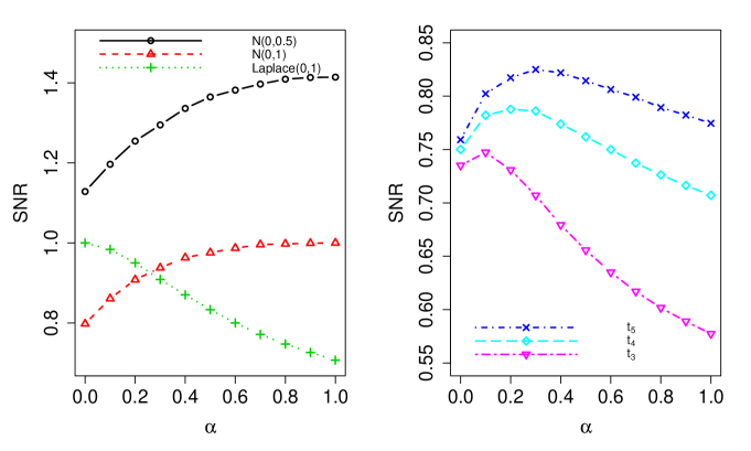
Figure 1: $SNR(\alpha,\widetilde{\bm{\tau}})$ under various errors with different weights $\alpha\in\{0,0.1,\ldots,0.9,1\}$ for the weighted loss with $\widetilde{\tau}=0.5$ and $K=1$.

For change point detection, a natural question is how to aggregate the $\mathbb{R}^{p}$–dimensional CUSUM process $\widetilde{\bm{C}}_{\alpha}(t;\widetilde{\bm{\tau}},\widehat{\bm{b}}_{\alpha},\widehat{\bm{\beta}}_{\alpha})$. Note that for high-dimensional sparse linear models, there are at most $s=s^{(1)}+s^{(2)}$ coordinates in $\bm{\beta}^{(1)}-\bm{\beta}^{(2)}$ that can have a change point, which can be much smaller than the data dimension $p$, although we allow $s$ to grow with the sample size $n$. Motivated by this, in this paper, we aggregate the first $s_{0}$ largest statistics of $\widetilde{\bm{C}}_{\alpha}(t;\widetilde{\bm{\tau}},\widehat{\bm{b}}_{\alpha},\widehat{\bm{\beta}}_{\alpha})$. To that end, we introduce the $(s_{0},2)$-norm as follows. Let $\bm{v}=(v_{1},\ldots,v_{p})\in\mathbb{R}^{p}$. For any $1\leq s_{0}\leq p$, define $\big{\|}\bm{v}\big{\|}_{(s_{0},2)}=(\sum_{j=1}^{s_{0}}|v_{(j)}|^{2})^{1/2}$, where $|v_{(1)}\geq|v_{(2)}|\cdots\geq|v_{(p)}|$ are the order statistics of $\bm{v}$. By definition, we can see that $\|\bm{v}\|_{(s_{0},2)}$ is the $L_{2}$-norm for the first $s_{0}$ largest order statistics of $(|v_{1}|,\ldots,|v_{p}|)^{\top}$, which can be regarded as an adjusted $L_{2}$-norm in high dimensions. Note that the $(s_{0},2)$-norm is a special case of the $(s_{0},\widetilde{p})$-norm proposed in Zhou et al. (2018) by setting $\widetilde{p}=2$. We also remark that taking the first $s_{0}$ largest order statistics can account for the sparsity structure of $\bm{\beta}^{(1)}-\bm{\beta}^{(2)}$. Using the $(s_{0},2)$-norm with a user-specified $s_{0}$ and known variance $\sigma^{2}(\alpha,\widetilde{\tau})$, we introduce the oracle individual testing statistic with respect to a given $\alpha\in[0,1]$ as

$$\widetilde{T}_{\alpha}=\max_{q_{0}\leq t\leq 1-q_{0}}\Big{\|}\widetilde{\bm{C}}_{\alpha}(t;\widetilde{\bm{\tau}},\widehat{\bm{b}}_{\alpha},\widehat{\bm{\beta}}_{a})\Big{\|}_{(s_{0},2)},\leavevmode\nobreak\ \leavevmode\nobreak\ \text{with}\leavevmode\nobreak\ \leavevmode\nobreak\ \alpha\in[0,1].\vspace{-0.2in}$$

By construction, $\widetilde{T}_{\alpha}$ can capture the tail structure of the underlying regression errors by choosing a special $\alpha$ and $\widetilde{\bm{\tau}}$. Specifically, for $\alpha=1$, it equals to the least square loss-based method. In this case, since $\widetilde{T}_{\alpha}$ only uses the moment information of the errors, it is powerful for detecting a change point with light-tailed errors such as Gaussian or sub-Gaussian distributions. For $\alpha=0$, $\widetilde{T}_{\alpha}$ reduces to the composite quantile loss-based method, which only uses the information of ranks or quantiles. In this case, $\widetilde{T}_{\alpha}$ is more robust to data with heavy tails such as Cauchy distributions. As a special case of $\alpha=0$, if we further choose $\widetilde{\tau}=0.5$ and $K=1$, our testing statistic reduces to the median regression-based method. Moreover, if we choose a proper non-trivial weight $\alpha$, $\widetilde{T}_{\alpha}$ enjoys satisfactory power performance for data with a moderate magnitude of tails such as the Student’s $t_{v}$ or Laplace distributions. Hence, our proposed individual testing statistics can adequately capture the tail structures of the data by choosing a proper combination of $\alpha$ and $\widetilde{\bm{\tau}}$.

Another distinguishing feature for using $\widetilde{T}_{\alpha}$ is that, we can establish a general and flexible framework for aggregating the score based CUSUM for high-dimensional sparse linear models. Instead of taking the $\ell_{\infty}$-norm as most papers adopted for making statistical inference of high-dimensional linear models (e.g., Xia et al., 2018), we choose to aggregate them via using the $\ell_{2}$-norm of the first $s_{0}$ largest order statistics. Under this framework, the $\ell_{\infty}$-norm is a special case by taking $s_{0}=1$. Moreover, as shown by our extensive numerical studies, choosing $s_{0}>1$ is more powerful for detecting sparse alternatives, and can significantly improve the detection powers as well as the estimation accuracy for change points, compared to using $s_{0}=1$.

2.2 Variance estimation under $\mathbf{H}_{0}$ and $\mathbf{H}_{1}$

Note that $\widetilde{T}_{\alpha}$ is constructed using a known variance $\sigma^{2}(\alpha,\widetilde{\bm{\tau}})$ which is defined in (2.14). In practice, however, $\sigma^{2}(\alpha,\widetilde{\bm{\tau}})$ is typically unknown. Hence, to yield a powerful testing method, a consistent variance estimation is needed especially under the alternative hypothesis. For high-dimensional change point analysis, the main difficulty comes from the unknown change point $t_{1}$. To overcome this problem, we propose a weighted variance estimation. In particular, for each fixed $\alpha\in[0,1]$ and $t\in(0,1)$, define the score based CUSUM statistic without standardization as follows:

$$\breve{\bm{C}}_{\alpha}(t;\widetilde{\bm{\tau}},\widehat{\bm{b}}_{\alpha},\widehat{\bm{\beta}}_{\alpha})=\dfrac{1}{\sqrt{n}}\big{(}\sum\limits_{i=1}^{\lfloor nt\rfloor}\bm{Z}_{\alpha}(\bm{X}_{i},Y_{i};\widetilde{\bm{\tau}},\widehat{\bm{b}}_{\alpha},\widehat{\bm{\beta}}_{\alpha})-\dfrac{\lfloor nt\rfloor}{n}\sum\limits_{i=1}^{n}\bm{Z}_{\alpha}(\bm{X}_{i},Y_{i};\widetilde{\bm{\tau}},\widehat{\bm{b}}_{\alpha},\widehat{\bm{\beta}}_{\alpha})\big{)}.\vspace{-0.2in}$$ (2.16)

Then, for each $\alpha\in[0,1]$, we obtain the individual based estimation for the change point:

$$\widehat{t}_{\alpha}=\mathop{\text{\rm arg\,max}}_{q_{0}\leq t\leq 1-q_{0}}\big{\|}\breve{\bm{C}}_{\alpha}(t;\widetilde{\bm{\tau}},\widehat{\bm{b}}_{\alpha},\widehat{\bm{\beta}}_{\alpha})\big{\|}_{(s_{0},2)}.\vspace{-0.2in}$$ (2.17)

In Theorem 3.5, we prove that under some regular conditions, if $\mathbf{H}_{1}$ holds, $\widehat{t}_{\alpha}$ is a consistent estimator for $t_{1}$, e.g. $|n\widehat{t}_{\alpha}-nt_{1}|=o_{p}(n)$. This result enables us to propose a variance estimator which is consistent under both $\mathbf{H}_{0}$ and $\mathbf{H}_{1}$. Specifically, let $h\in(0,1)$ be a user specified constant, and define the samples $n_{-}=\{i:i\leq nh\widehat{t}_{\alpha}\}$ and $n_{+}=\{i:\widehat{t}_{\alpha}n+(1-h)(1-\widehat{t}_{\alpha})n\leq i\leq n\}$. Let $((\widehat{\bm{b}}^{(1)}_{\alpha})^{\top},(\widehat{\bm{\beta}}^{(1)}_{\alpha})^{\top})$ and $((\widehat{\bm{b}}^{(2)}_{\alpha})^{\top},(\widehat{\bm{\beta}}^{(2)}_{\alpha})^{\top})$ be the estimators using the samples in $n_{-}$ and $n_{+}$. For each $\alpha\in[0,1]$, we can calculate the regression residuals:

$$\widehat{\epsilon}_{i}=(Y_{i}-\bm{X}_{i}^{\top}\widehat{\bm{\beta}}_{\alpha}^{(1)})\mathbf{1}\{i\in n_{-}\}+(Y_{i}-\bm{X}_{i}^{\top}\widehat{\bm{\beta}}_{\alpha}^{(2)})\mathbf{1}\{i\in n_{+}\},\leavevmode\nobreak\ \text{for}\leavevmode\nobreak\ i\in n_{-}\cup n_{+}.$$ (2.18)

Moreover, compute $\widehat{e}_{i}(\widetilde{\bm{\tau}})=K^{-1}\sum\limits_{k=1}^{K}\widehat{e}_{i}(\tau_{k})$ with $\widehat{e}_{i}(\tau_{k})$ defined as

$$\small\widehat{e}_{i}(\tau_{k}):=(\mathbf{1}\{\widehat{\epsilon}_{i}\leq\widehat{b}_{\alpha,k}^{(1)}\}-\tau_{k})\mathbf{1}\{i\in n_{-}\}+(\mathbf{1}\{\widehat{\epsilon}_{i}\leq\widehat{b}_{\alpha,k}^{(2)}\}-\tau_{k})\mathbf{1}\{i\in n_{+}\},\leavevmode\nobreak\ \text{for}\leavevmode\nobreak\ i\in n_{-}\cup n_{+}.$$ (2.19)

Lastly, based on $\widehat{\epsilon}_{i}$ and $\widehat{e}_{i}(\widetilde{\bm{\tau}})$, we can construct our weighted estimator for $\sigma^{2}(\alpha,\widetilde{\bm{\tau}})$ as

$$\widehat{\sigma}^{2}(\alpha,\widetilde{\bm{\tau}})=\widehat{t}_{\alpha}\times\widehat{\sigma}_{-}^{2}(\alpha,\widetilde{\bm{\tau}})+(1-\widehat{t}_{\alpha})\times\widehat{\sigma}_{+}^{2}(\alpha,\widetilde{\bm{\tau}}),\vspace{-0.2in}$$ (2.20)

where:

$$\widehat{\sigma}_{-}^{2}(\alpha,\widetilde{\bm{\tau}}):=\dfrac{1}{|n_{-}|}\sum_{i\in n_{-}}\big{[}(1-\alpha)\widehat{e}_{i}(\widetilde{\bm{\tau}})-\alpha\widehat{\epsilon}_{i}\big{]}^{2},\leavevmode\nobreak\ \leavevmode\nobreak\ \widehat{\sigma}_{+}^{2}(\alpha,\widetilde{\bm{\tau}}):=\dfrac{1}{|n_{+}|}\sum_{i\in n_{+}}\big{[}(1-\alpha)\widehat{e}_{i}(\widetilde{\bm{\tau}})-\alpha\widehat{\epsilon}_{i}\big{]}^{2}.\vspace{-0.2in}$$

For the above variance estimation, we can prove that $|\widehat{\sigma}^{2}(\alpha,\widetilde{\bm{\tau}})-{\sigma}^{2}(\alpha,\widetilde{\bm{\tau}})|=o_{p}(1)$ under either $\mathbf{H}_{0}$ or $\mathbf{H}_{1}$. As a result, the proposed variance estimator $\widehat{\sigma}^{2}(\alpha,\widetilde{\bm{\tau}})$ avoids the problem of non-monotonic power performance as discussed in Shao and Zhang (2010), which is a serious issue in change point analysis. Hence, we replace ${\sigma}(\alpha,\widetilde{\bm{\tau}})$ in (2.9) by $\widehat{\sigma}(\alpha,\widetilde{\bm{\tau}})$ and define the data-driven score-based CUSUM process $\{{\bm{C}}_{\alpha}(t;\widetilde{\bm{\tau}},\widehat{\bm{b}}_{\alpha},\widehat{\bm{\beta}}_{\alpha}),t\in[q_{0},1-q_{0}]\}$ with

$$\begin{array}[]{ll}{\bm{C}}_{\alpha}(t;\widetilde{\bm{\tau}},\widehat{\bm{b}}_{\alpha},\widehat{\bm{\beta}}_{\alpha})=\dfrac{1}{\sqrt{n}\widehat{\sigma}(\alpha,\widetilde{\bm{\tau}})}\big{(}\sum\limits_{i=1}^{\lfloor nt\rfloor}\bm{Z}_{\alpha}(\bm{X}_{i},Y_{i};\widetilde{\bm{\tau}},\widehat{\bm{b}}_{\alpha},\widehat{\bm{\beta}}_{\alpha})-\dfrac{\lfloor nt\rfloor}{n}\sum\limits_{i=1}^{n}\bm{Z}_{\alpha}(\bm{X}_{i},Y_{i};\widetilde{\bm{\tau}},\widehat{\bm{b}}_{\alpha},\widehat{\bm{\beta}}_{\alpha})\big{)}.\end{array}\vspace{-0.2in}$$ (2.21)

Note that we call ${\bm{C}}_{\alpha}(t;\widetilde{\bm{\tau}},\widehat{\bm{b}}_{\alpha},\widehat{\bm{\beta}}_{\alpha})$ data-driven since there are no unknown parameters in the testing statistic. For a user-specified $s_{0}\in\{1,\ldots,p\}$ and any $\alpha$, we define the final individual-based testing statistic as follows:

$${T}_{\alpha}=\max_{q_{0}\leq t\leq 1-q_{0}}\Big{\|}{\bm{C}}_{\alpha}(t;\widetilde{\bm{\tau}},\widehat{\bm{b}}_{\alpha},\widehat{\bm{\beta}}_{a})\Big{\|}_{(s_{0},2)},\leavevmode\nobreak\ \leavevmode\nobreak\ \text{with}\leavevmode\nobreak\ \leavevmode\nobreak\ \alpha\in[0,1].\vspace{-0.2in}$$ (2.22)

Throughout this paper, we use $\{{T}_{\alpha},\alpha\in[0,1]\}$ as our individual-based testing statistics.

2.3 Bootstrap approximation for the individual testing statistic

In high dimensions, it is very difficult to obtain the limiting null distribution of $T_{\alpha}$. To overcome this problem, we propose a novel bootstrap procedure. In particular, suppose we implement the bootstrap procedure for $B$ times. Then, for each $b$-th bootstrap with $b=1,\ldots,B$, we generate i.i.d. random variables $e_{1}^{b},\ldots,e_{n}^{b}$ with $e_{i}^{b}\sim N(0,1)$. Let $e_{i}^{b}(\widetilde{\bm{\tau}})=K^{-1}\sum\limits_{k=1}^{K}e_{i}^{b}(\tau_{k})$ with $e_{i}^{b}(\tau_{k}):=\mathbf{1}\{\epsilon_{i}^{b}\leq\Phi^{-1}(\tau_{k})\}-\tau_{k}$, where $\Phi(x)$ is the CDF for the standard normal distribution. Then, for each individual-based testing statistic $T_{\alpha}$, with a user specified $s_{0}$, we define its $b$-th bootstrap sample-based score CUSUM process as:

$${\bm{C}}^{b}_{\alpha}(t;\widetilde{\bm{\tau}})=\dfrac{1}{\sqrt{n}v(\alpha,\widetilde{\bm{\tau}})}\big{(}\sum\limits_{i=1}^{\lfloor nt\rfloor}\bm{X}_{i}((1-\alpha)e^{b}_{i}(\widetilde{\bm{\tau}})-\alpha e^{b}_{i})-\dfrac{\lfloor nt\rfloor}{n}\sum\limits_{i=1}^{n}\bm{X}_{i}((1-\alpha)e^{b}_{i}(\widetilde{\bm{\tau}})-\alpha e^{b}_{i})\big{)},\vspace{-0.2in}$$ (2.23)

where $v^{2}(\alpha,\widetilde{\bm{\tau}})$ is the corresponding variance for the bootstrap-based sample with

$$v^{2}(\alpha,\widetilde{\bm{\tau}}):=(1-\alpha)^{2}\text{Var}[e_{i}^{b}(\widetilde{\bm{\tau}})]+\alpha^{2}-2\alpha(1-\alpha)\text{Cov}(e_{i}^{b}(\widetilde{\bm{\tau}}),e^{b}_{i}).\vspace{-0.2in}$$ (2.24)

Note that for bootstrap, the calculation or estimation of $v^{2}(\alpha,\widetilde{\bm{\tau}})$ is not a difficult task since we use $N(0,1)$ as the error term. For example, when $\widetilde{\tau}=0.5$, it has an explicit form of

$$v^{2}(\alpha,\widetilde{\bm{\tau}})=(1-\alpha)^{2}\sum\limits_{k_{1}=1}^{K}\sum\limits_{k_{2}=1}^{K}\gamma_{k_{1}k_{2}}+\alpha^{2}-\alpha(1-\alpha)\sqrt{\dfrac{2}{\pi}}.\vspace{-0.2in}$$

Hence, for simplicity, we directly use the oracle variance $v^{2}(\alpha,\widetilde{\bm{\tau}})$ in (2.23). Using ${\bm{C}}^{b}_{\alpha}(t;\widetilde{\bm{\tau}})$ and for a user specified $s_{0}$, we define the $b$-th bootstrap version of the individual-based testing statistic $T_{\alpha}$ as

$$T_{\alpha}^{b}=\max_{q_{0}\leq t\leq 1-q_{0}}\Big{\|}\bm{C}^{b}_{\alpha}(t;\widetilde{\bm{\tau}})\Big{\|}_{(s_{0},2)},\leavevmode\nobreak\ \leavevmode\nobreak\ \text{with}\leavevmode\nobreak\ \leavevmode\nobreak\ \alpha\in[0,1].\vspace{-0.2in}$$ (2.25)

Let $\gamma\in(0,0.5)$ be the significance level. For each individual-based testing statistic $T_{\alpha}$, let $F_{\alpha}={\mathbb{P}}(T_{\alpha}\leq t)$ be its theoretical CDF and $P_{\alpha}=1-F_{\alpha}(T_{\alpha})$ be its theoretical $p$-value. Using the bootstrap samples $\{T_{\alpha}^{1},\ldots,T_{\alpha}^{B}\}$, we estimate $P_{\alpha}$ by

$$\widehat{P}_{\alpha}=\dfrac{\sum_{b=1}^{B}\mathbf{1}\{T_{\alpha}^{b}>T_{\alpha}|\mathcal{X},\mathcal{Y}\}}{B+1},\leavevmode\nobreak\ \leavevmode\nobreak\ \text{with}\leavevmode\nobreak\ \leavevmode\nobreak\ \alpha\in[0,1].\vspace{-0.15in}$$ (2.26)

Given the significance level $\gamma$, we can construct the individual test as

$$\Psi_{\gamma,\alpha}=\mathbf{1}\{\widehat{P}_{\alpha}\leq\gamma\},\leavevmode\nobreak\ \leavevmode\nobreak\ \text{with}\leavevmode\nobreak\ \leavevmode\nobreak\ \alpha\in[0,1].\vspace{-0.2in}$$ (2.27)

For each $T_{\alpha}$, we reject $\mathbf{H}_{0}$ if and only if $\Psi_{\gamma,\alpha}=1$. Note that the above bootstrap procedure is easy to implement since it does not require any model fitting such as obtaining the LASSO estimators which is required by the data-based testing statistic $T_{\alpha}$.

2.4 Constructing the tail-adaptive testing procedure

Algorithm 1 : A bootstrap procedure to obtain the tail-adaptive testing statistic $T_{\rm ad}$

Input:

Given the data $(\mathcal{X},\mathcal{Y})=\{(\bm{X}_{1},Y_{1}),\ldots,(\bm{X}_{n},Y_{n})\}$, set the values for $\widetilde{\bm{\tau}}$, $s_{0}$, $q_{0}$, the bootstrap replication number $B$, and the candidate subset $\mathcal{A}\subset[0,1]$.

Step 1:

Calculate the individual-based testing stastisic $T_{\alpha}$ for $\alpha\in\mathcal{A}$ as defined in (2.22).

Step 2:

For each $\alpha\in\mathcal{A}$, repeat the procedure (2.23) – (2.25) for $B$ times, and obtain the bootstrap samples $\{T_{\alpha}^{1},\ldots,T_{\alpha}^{B}\}$ for $\alpha\in\mathcal{A}$.

Step 3:

Based on the bootstrap samples in Step 2, calculate empirical $P$-values $\widehat{P}_{\alpha}$ for $\alpha\in\mathcal{A}$ as defined in (2.26).

Step 4:

Using $\widehat{P}_{\alpha}$ with $\alpha\in\mathcal{A}$, calculate the tail-adaptive testing statistic $T_{\rm ad}$ in (2.28).

Output:

Algorithm 1 provides the bootstrap based samples $\{T_{\alpha}^{1},\ldots,T_{\alpha}^{B}\}$ for $\alpha\in\mathcal{A}$, and the tail-adaptive testing statistic $T_{\rm ad}$.

In Sections 2.1 – 2.3, we propose a family of individual-based testing statistics $\{T_{\alpha},\alpha\in[0,1]\}$ and introduce a bootstrap-based procedure for approximating their theoretical $p$-values. As discussed in Sections 2.1 and seen from Figure 1, $T_{\alpha}$ with different $\alpha$’s can have various power performance for a given underlying error distribution. For example, $T_{\alpha}$ with a larger $\alpha$ (e.g. $\alpha=1$) is more sensitive to change points with light-tailed error distributions by using more moment information. In contrast, $T_{\alpha}$ with a smaller $\alpha$ (e.g. $\alpha=0,0.1$) is more powerful for data with heavy tails such as Student’s $t_{v}$ or even Cauchy distribution. In general, as shown in Figure 1, a properly chosen $\alpha$ can give the most satisfactory power performance for data with a particular magnitude of tails. In practice, however, the tail structures of data are typically unknown. Hence, it is desirable to construct a tail-adaptive method which is simultaneously powerful under various tail structures of data. One candidate method is to find $\alpha^{*}$ which maximizes the theoretical $SNR(\alpha,\widetilde{\bm{\tau}})$, i.e. $\alpha^{*}=\mathop{\text{\rm arg\,max}}_{\alpha}SNR(\alpha,\widetilde{\bm{\tau}})$, and constructs a corresponding individual testing statistic $T_{\alpha^{*}}$. Note that in theory, calculating $SNR(\alpha,\widetilde{\bm{\tau}})$ needs to know $\sigma(\alpha,\widetilde{\bm{\tau}})$ and $\{f_{\epsilon}(b_{k}^{(0)}),k=1,\ldots,K\}$, which could be difficult to estimate especially under the high-dimensional change point model. Instead, we construct our tail-adaptive method by combining all candidate individual tests for yielding a powerful one. In particular, as a small $p$-value leads to rejection of $\mathbf{H}_{0}$, for the individual tests $T_{\alpha}$ with $\alpha\in[0,1]$, we construct the tail-adaptive testing statistic as their minimum $p$-value, which is defined as follows:

$$T_{\rm ad}=\min_{\alpha\in\mathcal{A}}\widehat{P}_{\alpha},\vspace{-0.2in}$$ (2.28)

where $\widehat{P}_{\alpha}$ is defined in (2.26), and $\mathcal{A}$ is a candidate subset of $\alpha$.

In this paper, we require $|\mathcal{A}|$ to be finite, which is a theoretical requirement. Note that our tail-adaptive method is flexible and user-friendly. In practice, if the users have some prior knowledge about the tails of errors, we can choose $\mathcal{A}$ accordingly. For example, we can choose $\mathcal{A}=\{0.9,1\}$ for light-tailed errors, and $\mathcal{A}=\{0\}$ for extreme heavy tails such as Cauchy distributions. However, if the tail structure is unknown, we can choose $\mathcal{A}$ consisting both small and large values of $\alpha\in[0,1]$. For example, according to our theoretical analysis of $SNR(\alpha,\widetilde{\bm{\tau}})$, we find that $SNR(\alpha,\widetilde{\bm{\tau}})$ tends to be maximized near the boundary of $[0,1]$. Hence, we recommend to use $\mathcal{A}=\{0,0.1,0.5,0.9,1\}$ in real applications, which is shown by our numerical studies to enjoy stable size performance as well as high powers across various error distributions. Algorithm 1 describes our procedure to construct $T_{\rm ad}$. Using Algorithm 1, we construct the tail-adaptive testing statistic $T_{\rm ad}$. Let $F_{\rm ad}(x)$ be its theoretical distribution function. Note that $F_{\rm ad}(x)$ is unknown. Hence, we can not use $T_{\rm ad}$ directly for Problem (1.2). To approximate its theoretical $p$-value, we adopt the low-cost bootstrap method proposed by Zhou et al. (2018), which is also used in Liu et al. (2020). Let $\widehat{P}_{\rm ad}$ be an estimation for the theoretical $p$-value of $T_{\rm ad}$ using the low-cost bootstrap. Given the significance level $\gamma\in(0,0.5)$, define the final tail-adaptive test as:

$$\begin{array}[]{lc}\Psi_{\gamma,\rm ad}=\mathbf{1}\{\widehat{P}_{\rm ad}\leq\gamma\}.\end{array}\vspace{-0.2in}$$ (2.29)

For the tail-adaptive testing procedure, given $\gamma$, we reject $\mathbf{H}_{0}$ if $\Psi_{\gamma,\rm ad}=1$. If $\mathbf{H}_{0}$ is rejected by our tail-adaptive test, letting $\widehat{\alpha}=\mathop{\text{\rm arg\,min}}_{\alpha\in\mathcal{A}}\widehat{P}_{\alpha}$, we return the change point estimation as $\widehat{t}_{\rm ad}=\widehat{t}_{\widehat{\alpha}}$. As shown by our theory, under some conditions, we have $|\widehat{t}_{\rm ad}-t_{1}|=o_{p}(1)$.

2.5 Multiple change point detection

Algorithm 2 : A WBS-typed tail-adaptive test for multiple change point detection

Input:

Given the data $(\mathcal{X},\mathcal{Y})=\{(\bm{X}_{1},Y_{1}),\ldots,(\bm{X}_{n},Y_{n})\}$, set the values for $\widetilde{\bm{\tau}}$, the significance level $\gamma$, $s_{0}$, $q_{0}$, the bootstrap replication number $B$, the candidate subset $\mathcal{A}\subset[0,1]$, and a set of random intervals $\{(s_{\nu},e_{\nu}\}_{\nu=1}^{V}$ with thresholds $v_{0}$ and $v_{1}$. Initialize an empty set $\mathcal{C}$.

Step 1:

For each $\nu=1,\cdots,V$, compute $\widehat{P}_{\rm ad}(s_{\nu},e_{\nu})$ following Section 2.4.

Step 2:

Perform the following function with $S=q_{0}$ and $E=1-q_{0}$.

Function(S, E):

$S$ and $E$ are the starting and ending points for the change point detection.

1. RETURN if $E-S\leq v_{1}$.

2. Define $\mathcal{M}=\{1\leq\nu\leq V\,|\,[s_{\nu},e_{\nu}]\subset[E,S]\}$.

3. Compute the test statistics as $\overline{P}_{\rm ad}=\underset{\nu\in\mathcal{M},v_{0}\leq e_{\nu}-s_{\nu}}{\min}\widehat{P}_{\rm ad}(s_{\nu},e_{\nu})$ and the corresponding optimal solution $\nu^{\ast}$.

4. If $\overline{P}_{\rm ad}\geq\gamma/V$, RETURN. Otherwise, add the corresponding change point estimator $\widehat{t}_{\nu^{\ast}}$ to $\mathcal{C}$, and perform Function(S, $\nu^{\ast}$) and Function($\nu^{\ast}$, E).

Output:

The set of multiple change points $\mathcal{C}$.

In practical applications, it may exist multiple change points in describing the relationship between $\bm{X}$ and $Y$. Therefore, it is essential to perform estimation of multiple change points if $\mathbf{H}_{0}$ is rejected by our powerful tail-adaptive test. In this section, we extend our single change point detection method by the idea of WBS proposed in Fryzlewicz (2014) to estimate the locations of all possible multiple change points.

Consider a single change point detection task in any interval $[s,e]$, where $0\leq q_{0}\leq s<e\leq 1-q_{0}$. Following Section 2.4, we can compute the corresponding adaptive test statistics as $\widehat{P}_{\rm ad}(s,e)$ using the subset of our data, i.e., $\{\bm{X}_{\lfloor ns\rfloor},\bm{X}_{\lfloor ns\rfloor+1},\cdots,\bm{X}_{\lfloor ne\rfloor}\}$ and $\{Y_{\lfloor ns\rfloor},Y_{\lfloor ns\rfloor+1},\cdots,Y_{\lfloor ne\rfloor}\}$. Following the idea of WBS, we first independently generate a series of random intervals by the uniform distribution. Denote the number of these random intervals as $V$. For each random interval $[s_{\nu},e_{\nu}]$ among $\nu=1,2,\cdots,V$, we compute $\widehat{P}_{\rm ad}(s_{\nu},e_{\nu})$ as long as $0\leq q_{0}\leq s_{\nu}<e_{\nu}\leq 1-q_{0}$ and $e_{\nu}-s_{\nu}\geq v_{0}$, where $v_{0}$ is the minimum length for implementing Section 2.4. The threshold $v_{0}$ is used to reduce the variability of our algorithm for multiple change point detection. Based on the test statistics computed from the random intervals, we consider the final test statistics as $\overline{P}_{\rm ad}=\underset{1\leq\nu\leq V,v_{0}\leq e_{\nu}-s_{\nu}}{\min}\widehat{P}_{\rm ad}(s_{\nu},e_{\nu})$, based on which we make decisions if there exists at least one change point among these intervals. We stop the algorithm if $\overline{P}_{\rm ad}\geq\bar{c}$, otherwise we report the change point estimation in $[s_{\nu^{\ast}},e_{\nu^{\ast}}]$, where $\nu^{\ast}\in\underset{1\leq\nu\leq V,v_{0}\leq e_{\nu}-s_{\nu}}{\mathop{\text{\rm arg\,min}}}\widehat{P}_{\rm ad}(s_{\nu},e_{\nu})$, and continue our algorithm. Given the first change point estimator denoted by $\widehat{t}_{\nu^{\ast}}$, we split our data into two folds, i.e., before and after the estimated change point. Then we apply the previous procedure on each fold of the data using the same set of the random intervals as long as it satisfies the constraints. We repeat this step until the algorithm stops returning the change point estimation. For each step, we choose $\bar{c}=\gamma/V$, where $\gamma$ is the significance level used in each single change point detection algorithm. While we do not have the theoretical guarantee of using $\bar{c}$ in the proposed algorithm for controlling the size, the selection of this constant is based on the idea of Bonferroni correction, which is conservative. The numerical experiments in the appendix demonstrate the superiority of our proposed method in detecting multiple change points. Nevertheless, it is interesting to study the asymptotic property of $\overline{P}_{\rm ad}$, which we leave for the future work. The full algorithm of the multiple change point detection can be found in Algorithm 2.

3 Theoretical results

In this section, we give theoretical results for our proposed methods. In Section 3.1, we provide some basic model assumptions. In Section 3.2, we discuss the theoretical properties of the individual testing methods with a fixed $\alpha$ such as the size, power and change point estimation. In Section 3.3, we provide the theoretical results for the tail-adaptive method.

3.1 Basic assumptions

We introduce some basic assumptions for deriving our main theorems. Before that, we introduce some notations. Let $e_{i}(\widetilde{\bm{\tau}}):=K^{-1}\sum\limits_{k=1}^{K}\big{(}\mathbf{1}\{\epsilon_{i}\leq b^{(0)}_{k}\}-\tau_{k}\big{)}:=K^{-1}\sum\limits_{k=1}^{K}e_{i}(\tau_{k})$. We set $\mathcal{V}_{s_{0}}:=\{\bm{v}\in\mathbb{S}^{p}:\|\bm{v}\|_{0}\leq s_{0}\}$, where $\mathbb{S}^{p}:=\{\bm{v}\in\mathbb{R}^{p}:\|\bm{v}\|=1\}$. For each $\alpha\in[0,1]$, we introduce $\uwave{\bm{\beta}}^{*}=((\bm{\beta}^{*})^{\top},(\bm{b}^{*})^{\top})^{\top}\in\mathbb{R}^{p+K}$ with $\bm{\beta}^{*}\in\mathbb{R}^{p}$, $\bm{b}^{*}=(b_{1}^{*},\ldots,b_{K}^{*})^{\top}\in\mathbb{R}^{K}$, where

$$\uwave{\bm{\beta}}^{*}:=\mathop{\text{\rm arg\,min}}_{\bm{\beta}\in\mathbb{R}^{p},\bm{b}\in\mathbb{R}^{K}}{\mathbb{E}}\Big{[}(1-\alpha)\dfrac{1}{n}\sum_{i=1}^{n}\dfrac{1}{K}\sum_{k=1}^{K}\rho_{\tau_{k}}(Y_{i}-b_{i}-\bm{X}_{i}^{\top}\bm{\beta})+\dfrac{\alpha}{2n}\sum_{i=1}^{n}(Y_{i}-\bm{X}_{i}^{\top}\bm{\beta})^{2}\Big{]}.\vspace{-0.2in}$$ (3.1)

Note that by definition, we can regard $\uwave{\bm{\beta}}^{*}$ as the true parameters under the population level with pooled samples. We can prove that under $\mathbf{H}_{0}$, $\uwave{\bm{\beta}}^{*}=((\bm{\beta}^{(0)})^{\top},(\bm{b}^{(0)})^{\top})^{\top}$ with $\bm{b}^{(0)}=(b_{1}^{(0)},\ldots,b_{K}^{(0)})^{\top}$. Under $\mathbf{H}_{1}$, $\uwave{\bm{\beta}}^{*}$ is generally a weighted combination of the parameters before the change point and those after the change point. For example, when $\alpha=1$, it has the explicit form of $\uwave{\bm{\beta}}^{*}=((t_{1}\bm{\beta}^{(1)}+t_{2}\bm{\beta}^{(2)})^{\top},(\bm{b}^{(0)})^{\top})^{\top}$. More discussions about $\uwave{\bm{\beta}}^{*}$ under our weighted composite loss function are provided in the appendix. With the above notations, we are ready to introduce our assumptions as follows:
Assumption A (Design matrix): The design matrix $\mathbf{X}$ has i.i.d rows $\{\bm{X}_{i}\}_{i=1}^{n}$. (A.1) Assume that there are positive constants $\kappa_{1}$ and $\kappa_{2}$ such that $\lambda_{\rm min}(\bm{\Sigma})\geq\kappa_{1}>0$ and $\lambda_{\rm max}(\bm{\Sigma})\leq\kappa_{2}<\infty$ hold. (A.2) There exists some constant $M\geq 1$ such that $\max_{1\leq i\leq n}\max_{1\leq j\leq p}|X_{ij}|\leq M$ almost surely for every $n$ and $p$.
Assumption B (Error distribution): The error terms $\{\epsilon_{i}\}_{i=1}^{n}$ are i.i.d. with mean zero and finite variance $\sigma_{\epsilon}^{2}$. There exist positive constants $c_{\epsilon}$ and $C_{\epsilon}$ such that $c^{2}_{\epsilon}\leq\text{Var}(\epsilon_{i})\leq C^{2}_{\epsilon}$ hold. In addition, $\epsilon_{i}$ is independent with $\bm{X}_{i}$ for $i=1,\ldots,n$.
Assumption C (Moment constraints): (C.1) There exists some constant $b>0$ such that ${\mathbb{E}}(\bm{v}^{\top}\bm{X}_{i}\epsilon_{i})^{2}\geq b$ and ${\mathbb{E}}(\bm{v}^{\top}\bm{X}_{i}e_{i}(\widetilde{\bm{\tau}}))^{2}\geq b$, for $\bm{v}\in\mathcal{V}_{s_{0}}$ and all $i=1,\ldots,n$. Moreover, assume that $\inf_{i,j}{\mathbb{E}}[X^{2}_{ij}]\geq b$ holds. (C.2) There exists a constant $K>0$ such that ${\mathbb{E}}|\epsilon_{i}|^{2+\ell}\leq K^{\ell}$, for $\ell=1,2$.
 Assumption D (Underlying distribution): The distribution function $\epsilon$ has a continuously differentiable density function $f_{\epsilon}(t)$ whose derivative is denoted by $f^{\prime}_{\epsilon}(t)$. Furthermore, suppose there exist some constants $C_{+}$, $C_{-}$ and $C^{\prime}_{+}$ such that

$$\begin{array}[]{l}\text{(D.1)}\sup\limits_{t\in\mathbb{R}}f_{\epsilon}(t)\leq C_{+};\leavevmode\nobreak\ \text{(D.2)}\inf\limits_{j=1,2}\inf\limits_{1\leq k\leq K}f_{\epsilon}(\bm{x}^{\top}(\bm{\beta}^{*}-\bm{\beta}^{(j)})+b_{k}^{*})\geq C_{-};\text{(D.3)}\sup\limits_{t\in\mathbb{R}}|f^{\prime}_{\epsilon}(t)|\leq C^{\prime}_{+}.\end{array}\vspace{-0.2in}$$

Assumption E (Parameter space): (E.1) We require $s_{0}^{3}\log(pn)=O(n^{\xi_{1}})$ for some $0<\xi_{1}<1/7$ and $s_{0}^{4}\log(pn)=O(n^{\xi_{2}})$ for some $0<\xi_{2}<\frac{1}{6}$. (E.2) Assume that $\dfrac{s_{0}^{2}s^{3}\log^{3}(pn)}{n}\rightarrow 0$ as $(n,p)\rightarrow\infty$. (E.3) For $\bm{\beta}^{(1)}$ and $\bm{\beta}^{(2)}$, we require $\max(\|\bm{\beta}^{(1)}\|_{\infty},\|\bm{\beta}^{(2)}\|_{\infty})<C_{\bm{\beta}}$ for some $C_{\bm{\beta}}>0$. Moreover, we require $\|\bm{\beta}^{(2)}-\bm{\beta}^{(1)}\|_{1}\leq C_{\bm{\Delta}}$ for some constant $C_{\bm{\Delta}}>0$. (E.4) For the tuning parameters $\lambda_{\alpha}$ in (2.8), we require $\lambda_{\alpha}=C_{\lambda}\sqrt{\log(pn)/n}$ for some $C_{\lambda}>0$.

Assumption A gives some conditions for the design matrix, requiring $\bm{X}$ has a non-degenerate covariance matrix $\bm{\Sigma}$ in terms of its eigenvalues. This is important for deriving the high-dimensional LASSO property with $\alpha\in[0,1]$ under both $\mathbf{H}_{0}$ and $\mathbf{H}_{1}$. Moreover, it also requires that $X_{ij}$ is bounded by some big constant $M>0$, which has been commonly used in the literature. Assumption B mainly requires the underlying error term $\epsilon_{i}$ has non-degenerate variance. Assumption C imposes some restrictions on the moments of the error terms as well as the design matrix. In particular, Assumption C.1 requires that $\bm{v}^{\top}\bm{X}\epsilon$, $\bm{v}^{\top}\bm{X}e(\widetilde{\bm{\tau}})$, as well as $X_{ij}$ have non-degenerate variances. Moreover, Assumption C.2 requires that the errors have at most fourth moments, which is much weaker than the commonly used Gaussian or sub-Gaussian assumptions. Both Assumptions C.1 and C.2 are basic moment conditions for bootstrap approximations for the individual-based tests. See Lemma C.6 in the appendix. Assumptions D.1 - D.3 are some regular conditions for the underlying distribution of the errors, requiring $\epsilon$ has a bounded density function as well as bounded derivatives. Assumption D.2 also requires the density function at $\bm{x}^{\top}(\bm{\beta}^{*}-\bm{\beta}^{(j)})+b_{k}^{*}$ to be strictly bounded away from zero. Lastly, Assumption E imposes some conditions for the parameter spaces in terms of $(s_{0},n,p,s,\bm{\beta}^{(1)},\bm{\beta}^{(2)})$. Specifically, Assumption E.1 scales the relationship between $s_{0}$, $n$, and $p$, which allows $s_{0}$ can grow with the sample size $n$. This condition is mainly used to establish the high-dimensional Gaussian approximation for our individual tests. Assumption E.2 also gives some restrictions on $(s_{0},s,n,p)$. Note that both Assumptions E.1 and E.2 allow the data dimension $p$ to be much larger than the sample size $n$ as long as the required conditions hold. Assumption E.3 requires that the regression coefficients as well as signal jump in terms of its $\ell_{1}$-norm are bounded. Assumption E.4 imposes the regularization parameter $\lambda_{\alpha}=O(\sqrt{\log(pn)/n})$, which is important for deriving the desired error bound for the LASSO estimators under both $\mathbf{H}_{0}$ and $\mathbf{H}_{1}$ using our weighted composite loss function. See Lemmas C.9 - C.11 in the appendix.

Remark 3.1.

Assumption C.2 with the finite fourth moment is mainly for the individual test with $\alpha=1$, while Assumption D without any moment constraints is for that with $\alpha=0$. Hence, our proposed individual-based change point method extends the high-dimensional linear models with sub-Gaussian distributed errors to those with only finite moments or without any moments, covering a wide range of errors with different tails.

Remark 3.2.

Our proposed individual method with $\alpha=0$ needs to cover both cases with and without a change point. To obtain the desired error bound of LASSO estimation, we require that $\inf\limits_{j=1,2}\inf\limits_{1\leq k\leq K}f_{\epsilon}(\bm{x}^{\top}(\bm{\beta}^{*}-\bm{\beta}^{(j)})+b_{k}^{*})\geq C_{-}$. This is different from the classical assumption (Zhao et al., 2014) that $\inf\limits_{1\leq k\leq K}f_{\epsilon}(b_{k}^{(0)})\geq C_{-}$. Note that our assumption is quite mild since essentially, it only requires that the density function is non-generate at a neighborhood of $b_{k}^{*}$ which is shown to be satisfied under Assumptions A.2 and E.3.

3.2 Theoretical results of the individual-based testing statistics

3.2.1 Validity of controlling the testing size

Before giving the size results, we first consider the variance estimation. Recall $\sigma^{2}(\alpha,\widetilde{\bm{\tau}})$ in (2.14) and $\widehat{\sigma}^{2}(\alpha,\widetilde{\bm{\tau}})$ in (2.20). Theorem 3.3 shows that the pooled weighted variance estimator $\widehat{\sigma}^{2}(\alpha,\widetilde{\bm{\tau}})$ is consistent under the null hypothesis, which is crucial for deriving the Gaussian approximation results as shown in Theorem 3.4 and shows that our testing method has satisfactory size performance.

Theorem 3.3.

For $\alpha=1$, suppose Assumptions A, B, C, E hold. For $\alpha=0$, suppose Assumptions A, C.1, D, E hold. For $\alpha\in(0,1)$, suppose Assumptions A - E hold. Let $r_{\alpha}(n)=\sqrt{s\log(pn)/n}$ if $\alpha=1$ and $r_{\alpha}(n)=s\sqrt{\dfrac{\log(pn)}{n}}\vee s^{\frac{1}{2}}(\dfrac{\log(pn)}{n})^{\frac{3}{8}}$ if $\alpha\in[0,1)$. Under $\mathbf{H}_{0}$, for each $\alpha\in[0,1]$, we have

$$|\widehat{\sigma}^{2}(\alpha,\widetilde{\bm{\tau}})-{\sigma}^{2}(\alpha,\widetilde{\bm{\tau}})|=O_{p}(r_{\alpha}(n)).\vspace{-0.2in}$$

Based on Theorem 3.3 as well as some other regularity conditions, the following Theorem 3.4 justifies the validity of our bootstrap-based procedure in Algorithm 1.

Theorem 3.4.

For $\alpha=1$, suppose Assumptions A, B, C, E hold. For $\alpha=0$, suppose Assumptions A, C.1, D, E hold. For $\alpha\in(0,1)$, suppose Assumptions A - E hold. Then, under $\mathbf{H}_{0}$, for the individual test with $\alpha\in[0,1]$, we have

$$\sup_{z\in(0,\infty)}\big{|}{\mathbb{P}}(T_{\alpha}\leq z)-{\mathbb{P}}(T_{\alpha}^{b}\leq z|\mathcal{X},\mathcal{Y})\big{|}=o_{p}(1),\leavevmode\nobreak\ \text{as}\leavevmode\nobreak\ n,p\rightarrow\infty.\vspace{-0.2in}$$ (3.2)

Theorem 3.4 demonstrates that we can uniformly approximate the distribution of $T_{\alpha}$ by that of $T_{\alpha}^{b}$. The following Corollary further shows that our proposed new test $\Psi_{\gamma,\alpha}$ can control the Type I error asymptotically for any given significant level $\gamma\in(0,1)$.

Corollary 3.1.

Suppose the assumptions in Theorem 3.4 hold. Under $\mathbf{H}_{0}$, we have

$${\mathbb{P}}(\Psi_{\gamma,\alpha}=1)\rightarrow\gamma,\leavevmode\nobreak\ \text{as}\leavevmode\nobreak\ n,p,B\rightarrow\infty.\vspace{-0.2in}$$

3.2.2 Change point estimation

After analyzing the theoretical results under the null hypothesis, we next consider the performance of the individual test under $\mathbf{H}_{1}$. We first give some theoretical results on the change point estimation. To that end, some additional assumptions are needed. Recall $\Pi=\{j:\beta^{(1)}_{j}\neq\beta^{(2)}_{j}\}$ as the set with change points. For $j\in\{1,\ldots,p\}$, define the signal jump $\bm{\Delta}=(\Delta_{1},\ldots,\Delta_{p})^{\top}$ with $\Delta_{j}:=\beta^{(1)}_{j}-\beta^{(2)}_{j}$. Let $\Delta_{\min}=\min_{j\in\Pi}|\Delta_{j}|$ and $\Delta_{\max}=\max_{j\in\Pi}|\Delta_{j}|$. With the above notations, we introduce the following Assumption F.
Assumption F. There exist constants $\underline{c}>0$ and $\overline{C}>0$ such that

$$0<\underline{c}\leq\liminf\limits_{p\rightarrow\infty}\dfrac{\Delta_{\min}}{\Delta_{\max}}\leq\limsup\limits_{p\rightarrow\infty}\dfrac{\Delta_{\max}}{\Delta_{\min}}\leq\overline{C}<\infty.\vspace{-0.2in}$$ (3.3)

Note that Assumption F is only a technical condition requiring that $\Delta_{\min}$ and $\Delta_{\max}$ are of the same order. With Assumption F as well as those of Assumptions A - E, Theorem 3.5 below provides a non-asymptotic estimation error bound of the argmax-based individual change point estimator $\widehat{t}_{\alpha}$ for $t_{1}$. To give a precise result, for change point estimation, we assume $s_{0}$ is fixed.

Theorem 3.5.

Suppose $\|\bm{\Delta}\|_{(s_{0},2)}\gg\sqrt{\log(pn)/n}$ and Assumption F hold. Moreover, For $\alpha=1$, suppose Assumptions A, B, C, E.2 - E.4 as well as $n^{1/4}=o(s)$ hold; For $\alpha=0$, suppose Assumptions A, C.1, D, E.2 - E.4 as well as

$$\lim\limits_{n,p\rightarrow\infty}s_{0}^{1/2}s^{2}\sqrt{\log(p)/n}\|\bm{\Delta}\|_{(s_{0},2)}=0\vspace*{-0.2in}$$

hold; For $\alpha\in(0,1)$, suppose Assumptions A, B, C, D, E.2 - E.4 as well as $n^{1/4}=o(s)$
and $\lim\limits_{n,p\rightarrow\infty}s_{0}^{1/2}s^{2}\sqrt{\log(pn)/n}\|\bm{\Delta}\|_{(s_{0},2)}=0$ hold. Then, under $\mathbf{H}_{1}$, for each $\alpha\in[0,1]$, with probability tending to one, we have

$$\big{|}\widehat{t}_{\alpha}-t_{1}\big{|}\leq C^{*}(s_{0},\widetilde{\bm{\tau}},\alpha)\dfrac{\log(pn)}{nSNR^{2}(\alpha,\widetilde{\bm{\tau}})\|\bm{\Sigma}\bm{\Delta}\|^{2}_{(s_{0},2)}},\vspace{-0.2in}$$ (3.4)

where $C^{*}(s_{0},\widetilde{\bm{\tau}},\alpha)>0$ is some universal constant only depending on $s_{0},\widetilde{\bm{\tau}}$ and $\alpha$.

Theorem 3.5 shows that our individual estimators are consistent under the condition $\|\bm{\Delta}\|_{(s_{0},2)}\gg\sqrt{\log(pn)/n}$. Moreover, according to Rinaldo et al. (2021), for high-dimensional linear models, under Assumption F, if $\|\bm{\Delta}\|_{\infty}\gg 1/\sqrt{n}$, any change point estimator $\widehat{t}$ has an estimation lower bound $|\widehat{t}-t_{1}|\geq c_{*}\dfrac{1}{n\|\bm{\Delta}\|^{2}_{\infty}}$, for some constant $c_{*}>0$. Hence, considering (3.3) and (3.4), with a fixed $s_{0}$, Theorem 3.5 demonstrates that our individual-based estimators for the change point are rate optimal up to a $\log(pn)$ factor. More importantly, our proposed estimators $\{\widehat{t}_{\alpha},\alpha\in[0,1]\}$ only require $O(\rm Lasso(n,p))$ operations to calculate, which is less computationally expensive than the grid search based method in Lee et al. (2016).

3.2.3 Power performance

We discuss the power properties of the individual tests. Note that for the change point problem, variance estimation under the alternative is a difficult but important task. As pointed out in Shao and Zhang (2010), due to the unknown change point, any improper estimation may lead to nonmonotonic power performance. This distinguishes the change point problem substantially from one-sample or two-sample tests where homogenous data are used to construct consistent variance estimation. Hence, for yielding a powerful change point test, we need to guarantee a consistent variance estimation. Theorem 3.6 shows that the pooled weighted variance estimation is consistent under $\mathbf{H}_{1}$. This guarantees that our proposed testing method has reasonable power performance.

Theorem 3.6.

Suppose the assumptions in Theorem 3.5 hold. Let $r_{\alpha}(n)=\sqrt{s\log(pn)/n}$ if $\alpha=1$ and $r_{\alpha}(n)=s\sqrt{\dfrac{\log(pn)}{n}}\vee s^{\frac{1}{2}}(\dfrac{\log(pn)}{n})^{\frac{3}{8}}$ if $\alpha\in[0,1)$. Under $\mathbf{H}_{1}$, for each $\alpha\in[0,1]$, we have

$$|\widehat{\sigma}^{2}(\alpha,\widetilde{\bm{\tau}})-{\sigma}^{2}(\alpha,\widetilde{\bm{\tau}})|=O_{p}(r_{\alpha}(n)).\vspace{-0.2in}$$

According to the proof of Theorem 3.6, several interesting observations can be drawn. Even if the signal strength is weak such as $\|\bm{\Delta}\|_{(s_{0},2)}=O(\sqrt{\log(pn)/n})$, the pooled weighted variance estimator $\widehat{\sigma}^{2}(\alpha,\widetilde{\bm{\tau}})$ can still be consistent for ${\sigma}^{2}(\alpha,\widetilde{\bm{\tau}})$. However, in this case, we can not guarantee that our change point estimator is consistent as $\|\bm{\Delta}\|_{(s_{0},2)}\gg\sqrt{\log(pn)/n}$ is required in Theorem 3.5 for consistency. In contrast, if the signal strength is strong enough such that $\|\bm{\Delta}\|_{(s_{0},2)}\gg\sqrt{\log(p)/n}$, then a consistent change point estimator such as the proposed $\widehat{t}_{\alpha}$ is needed to guarantee Theorem 3.6. These are insightful findings for variance estimation in change point analysis, which are not shown in the i.i.d. case.

Using the consistent variance estimation, we are able to discuss the power properties of the individual tests. To this end, we need some additional notations. Define the oracle signal to noise ratio vector $\bm{D}=(D_{1},\ldots,D_{p})^{\top}$ with

$$D_{j}:=\left\{\begin{array}[]{ll}0,&\text{for}\leavevmode\nobreak\ \leavevmode\nobreak\ j\in\Pi^{c}\\ SNR(\alpha,\widetilde{\bm{\tau}})\times\Big{|}{t_{1}(1-t_{1})\big{(}\bm{\Sigma}(\bm{\beta}^{(1)}-\bm{\beta}^{(2)})\big{)}_{j}}\Big{|},&\text{for}\leavevmode\nobreak\ \leavevmode\nobreak\ j\in\Pi,\end{array}\right.\vspace{-0.2in}$$ (3.5)

where $SNR(\alpha,\widetilde{\bm{\tau}})$ is defined in (2.11). With the above notations and some regularity conditions, Theorem 3.7 stated below shows that we can reject the null hypothesis of no change point with probability tending to $1$.

Theorem 3.7.

Let $\epsilon_{n}:=O(s^{1/2}_{0}s\sqrt{{\log(pn)}/{n}})\vee O({s_{0}^{1/2}s^{2}\sqrt{{\log(pn)}/{n}}\|\bm{\Delta}\|_{(s_{0},2)}})$. For each $\alpha\in[0,1]$, assume the following conditions hold: When $\alpha=1$, suppose that Assumptions A, B, C, E.2 - E.4 hold; When $\alpha=0$, suppose that Assumptions A, C.1, D, E.2 - E.4 as well as

$$\lim\limits_{n,p\rightarrow\infty}s_{0}^{1/2}s^{2}\sqrt{\log(p)/n}\|\bm{\Delta}\|_{(s_{0},2)}=0\vspace{-0.2in}$$ (3.6)

hold; When $\alpha\in(0,1)$, suppose that Assumptions A - D, E.2 - E.4 as well as (3.6) hold. Under $\mathbf{H}_{1}$, if $\bm{D}$ in (3.5) satisfies

$$\sqrt{n}\times\|\bm{D}\|_{(s_{0},2)}\geq\dfrac{C(\widetilde{\bm{\tau}},\alpha)}{1-\epsilon_{n}}s^{1/2}_{0}\big{(}\sqrt{\log(pn)}+\sqrt{\log(1/\gamma)}\big{)},\vspace{-0.2in}$$ (3.7)

then we have

$${\mathbb{P}}(\Phi_{\gamma,\alpha}=1)\rightarrow 1,\text{as}\leavevmode\nobreak\ n,p,B\rightarrow\infty,\vspace{-0.2in}$$

where $C(\widetilde{\bm{\tau}},\alpha)$ is some universal positive constant only depending on $\widetilde{\bm{\tau}}$ and $\alpha$.

Theorem 3.7 demonstrates that with probability tending to one, our proposed individual test with $\alpha\in[0,1]$ can detect the existence of a change point for high-dimensional linear models as long as the corresponding signal to noise ratio satisfies (3.7). Combining (3.5) and (3.7), for each individual test, we note that with a larger signal jump and a closer change point location $t_{1}$ to the middle of data observations, it is more likely to trigger a rejection of the null hypothesis. More importantly, considering $\epsilon_{n}=o(1)$, Theorem 3.7 illustrates that for consistently detecting a change point, we require the signal to noise ratio vector to be at least an order of $\|\bm{D}\|_{(s_{0},2)}\asymp s_{0}^{1/2}\sqrt{\log(pn)/n}$, which is particularly interesting to further discuss under several special cases. For example, if we choose $s_{0}=1$ and $\alpha=1$, our proposed individual test reduces to the least squared loss based testing statistic with the $\ell_{\infty}$-norm aggregation. In this case, we require $\|\bm{D}\|_{\infty}\asymp\sqrt{\log(pn)/n}$ for detecting a change point. If we choose $\alpha=0$ with the composite quantile loss, the test is still consistent as long as $\|\bm{D}\|_{\infty}\asymp\sqrt{\log(pn)/n}$. Note that the latter one is of special interest for the robust change point detection. Hence, our theorem provides the unified condition for detecting a change point under a general framework, which may be of independent interest. Moreover, Theorem 3.7 reveals that for detecting a change point, our individual-based method with $\alpha\in[0,1]$ can account for the tails of the data. For Model (2.1) with a fixed signal jump $\bm{\Delta}$ and a change point location $t_{1}$, considering (3.5) and (3.7), the individual test $T_{\alpha}$ is more powerful with a larger $SNR(\alpha,\widetilde{\bm{\tau}})$. This reveals why the individual tests with different weights $\alpha$ perform very differently under various error distributions.

Lastly, it is worth mentioning that the requirements for identifying and detecting a change point are different for Model (2.1). More specifically, for each individual-based method, Theorem 3.5 demonstrates that, to consistently estimate the location of $t_{1}$, the signal strength should at least satisfy $\|\bm{\Delta}\|_{(s_{0},2)}\gg\sqrt{\log(pn)/n}$. In contrast, Theorem 3.7 shows that we can detect a change point if $\|\bm{\Delta}\|_{(s_{0},2)}\geq C\sqrt{\log(pn)/n}$ holds. This reveals that we need more stringent conditions for localizing a change point than detecting its existence for high-dimensional linear models. To the best of our knowledge, this is still an open question on whether one can obtain consistent change point estimation if $\|\bm{\Delta}\|_{(s_{0},2)}=O(\sqrt{\log(pn)/n})$.

3.3 Theoretical results of the tail-adaptive testing statistics

In Section 3.2, we present the theoretical properties of the individual testing statistics $T_{\alpha}$ with $\alpha\in[0,1]$. In this section, we discuss the size and power properties of the tail-adaptive test $\Psi_{\gamma,\rm ad}$ defined in (2.29). To present the theorems, we need additional notations. Let $F_{T_{\alpha}}(x):={\mathbb{P}}(T_{\alpha}\leq x)$ be the CDF of $T_{\alpha}$. Then $\widehat{P}_{\alpha}$ in (2.26) approximates the following individual tests’ theoretical $P$-values defined as $P_{\alpha}:=1-F_{T_{\alpha}}(T_{\alpha})$. Hence, based on the above theoretical $P$-values, we can define the oracle tail-adaptive testing statistic $\widetilde{T}_{\rm ad}=\min_{\alpha\in\mathcal{A}}P_{\alpha}.$ Let $\widetilde{F}_{T,\rm ad}(x):={\mathbb{P}}(\widetilde{T}_{\rm ad}\leq x)$ be the CDF of $\widetilde{T}_{\rm ad}$. Then we can also define the theoretical tail-adaptive test’s $P$-value as $\widetilde{P}_{\rm ad}:=\widetilde{F}_{T,\rm ad}(\widetilde{T}_{\rm ad})$. Recall $\widehat{P}_{\rm ad}$ be the low cost bootstrap $P$-value for $\widetilde{P}_{\rm ad}$. In what follows, we show that $\widehat{P}_{\rm ad}$ converges to $\widetilde{P}_{\rm ad}$ in probability as $n,p,B\rightarrow\infty$.

We introduce Assumption $\mathbf{E.1^{\prime}}$ to describe the scaling relationships among $n$, $p$, and $s_{0}$. Let $\bm{G}_{i}=(G_{i1},\ldots,G_{ip})^{\top}$ with $\bm{G}_{i}\sim N(\mathbf{0},\bm{\Sigma})$ being i.i.d. Gaussian random vectors, where $\bm{\Sigma}:=\text{Cov}(\bm{X}_{1})$. Define

$$\bm{C}^{\bm{G}}(t)=\dfrac{1}{\sqrt{n}}\big{(}\sum_{i=1}^{\lfloor nt\rfloor}\bm{G}_{i}-\dfrac{\lfloor nt\rfloor}{n}\sum_{i=1}^{n}\bm{G}_{i}\big{)}\leavevmode\nobreak\ \leavevmode\nobreak\ \text{and}\leavevmode\nobreak\ \leavevmode\nobreak\ T^{\bm{G}}=\max_{q_{0}\leq t\leq 1-q_{0}}\|\bm{C}^{\bm{G}}(t)\|_{(s_{0},2)}.\vspace{-0.2in}$$

As shown in the proof of Theorem 3.4, we use $T^{\bm{G}}=\max\limits_{q_{0}\leq t\leq 1-q_{0}}\big{\|}\bm{C}^{\bm{G}}(t)\big{\|}_{(s_{0},2)}$ to approximate $T_{\alpha}$. For $T^{\bm{G}}$, let $f_{T^{\bm{G}}}(x)$ and $c_{T^{\bm{G}}}(\gamma)$ be the probability density function (pdf), and the $\gamma$-quantile of $T^{\bm{G}}$, respectively. We then define $h(\epsilon)$ as $h(\epsilon)=\max_{x\in I(\epsilon)}f_{T^{\bm{G}}}^{-1}(x)$, where $I(\epsilon):=[c_{T^{\bm{G}}}(\epsilon),c_{T^{\bm{G}}}(1-\epsilon)]$.

With the above definitions and notations, we now introduce Assumption $\mathbf{E.1^{\prime}}$:

(E.1)^′

For any $0<\epsilon<1$, we require $h^{0.6}(\epsilon)s_{0}^{3}\log(pn)=o(n^{1/10})$.

Note that Assumption $\mathbf{E.1^{\prime}}$ is more stringent than Assumption $\bf{E.1}$. The intuition of Assumption $\mathbf{E.1^{\prime}}$ is that, we construct our tail-adaptive testing statistic by taking the minimum $P$-values of the individual tests. For analyzing the combinational tests, we need not only the uniform convergence of the distribution functions, but also the uniform convergence of their quantiles on $[\epsilon,1-\epsilon]$ for any $0<\epsilon<1$.

The following Theorem 3.8 justifies the validity of the low-cost bootstrap procedure in Section 2.4. It also shows that our tail-adaptive test has the asymptotic level of $\gamma$.

Theorem 3.8.

For $T_{\rm ad}$, suppose Assumptions A - D, E.1^′, E.2 - E.4 hold. Under $\mathbf{H}_{0}$, we have

$$\begin{array}[]{lc}{\mathbb{P}}(\Psi_{\gamma,\rm ad}=1)\rightarrow\gamma,&\text{and}\leavevmode\nobreak\ \leavevmode\nobreak\ \widehat{P}_{\rm ad}-\widetilde{P}_{\rm ad}\xrightarrow{{\mathbb{P}}}0,\leavevmode\nobreak\ \text{as}\leavevmode\nobreak\ n,p,B\rightarrow\infty.\end{array}\vspace{-0.2in}$$

After analyzing the size, we now discuss the power. Theorem 3.9 shows that under some regularity conditions, our tail-adaptive test has its power converging to one.

Theorem 3.9.

Let $\epsilon_{n}:=O(s^{1/2}_{0}s\sqrt{{\log(pn)}/{n}})\vee O({s_{0}^{1/2}s^{2}\sqrt{{\log(pn)}/{n}}\|\bm{\Delta}\|_{(s_{0},2)}})$. Suppose Assumptions A - D, E.2 - E.4 as well as $\lim\limits_{n,p\rightarrow\infty}s_{0}^{1/2}s^{2}\sqrt{\log(p)/n}\|\bm{\Delta}\|_{(s_{0},2)}=0$ hold. If $\mathbf{H}_{1}$ holds with

$$\sqrt{n}\times\|\bm{D}\|_{(s_{0},2)}\geq\dfrac{C(\widetilde{\bm{\tau}},\alpha)}{1-\epsilon_{n}}s^{1/2}_{0}\big{(}\sqrt{\log(pn)}+\sqrt{\log(|\mathcal{A}|/\gamma)}\big{)},\vspace{-0.1in}$$ (3.8)

then for $T_{\rm ad}$, we have

$$\begin{array}[]{lc}{\mathbb{P}}(\Psi_{\gamma,\rm ad}=1)\rightarrow 1\leavevmode\nobreak\ \text{as}\leavevmode\nobreak\ n,p,B\rightarrow\infty,\end{array}\vspace{-0.2in}$$

where $C(\widetilde{\bm{\tau}},\alpha)$ is some universal positive constant only depending on $\widetilde{\bm{\tau}}$ and $\alpha$.

Note that based on the theoretical results obtained in Section 3.2, Theorems 3.8 and 3.9 can be proved using some modifications of the proofs of Theorems 3.5 and 3.7 in Zhou et al. (2018). Hence, we omit the detailed proofs for brevity. Lastly, recall the tail-adaptive based change point estimator $\widehat{t}_{\rm ad}=\widehat{t}_{\widehat{\alpha}}$ with $\widehat{\alpha}=\mathop{\text{\rm arg\,min}}_{\alpha\in\mathcal{A}}\widehat{P}_{\alpha}$. According to Theorem 3.5, the tail-adaptive estimator is consistent which is summarized as a corollary.

Corollary 3.2.

Suppose Assumptions A - D, E.2 - E.4, F as well as $n^{1/4}=o(s)$ and
$\lim\limits_{n,p\rightarrow\infty}s_{0}^{1/2}s^{2}\sqrt{\log(pn)/n}\|\bm{\Delta}\|_{(s_{0},2)}=0$ hold. Suppose additionally $\|\bm{\Delta}\|_{(s_{0},2)}\gg\sqrt{\dfrac{\log(pn)}{n}}$ holds. Under $\mathbf{H}_{1}$, with probability tending to one, we have

$$\big{|}\widehat{t}_{\rm ad}-t_{1}\big{|}\leq C_{\rm ad}\dfrac{\log(pn)}{n\|\bm{\Sigma}\bm{\Delta}\|^{2}_{(s_{0},2)}},\vspace{-0.2in}$$

where $C_{\rm ad}>0$ is some universal constant not depending on $n$ or $p$.

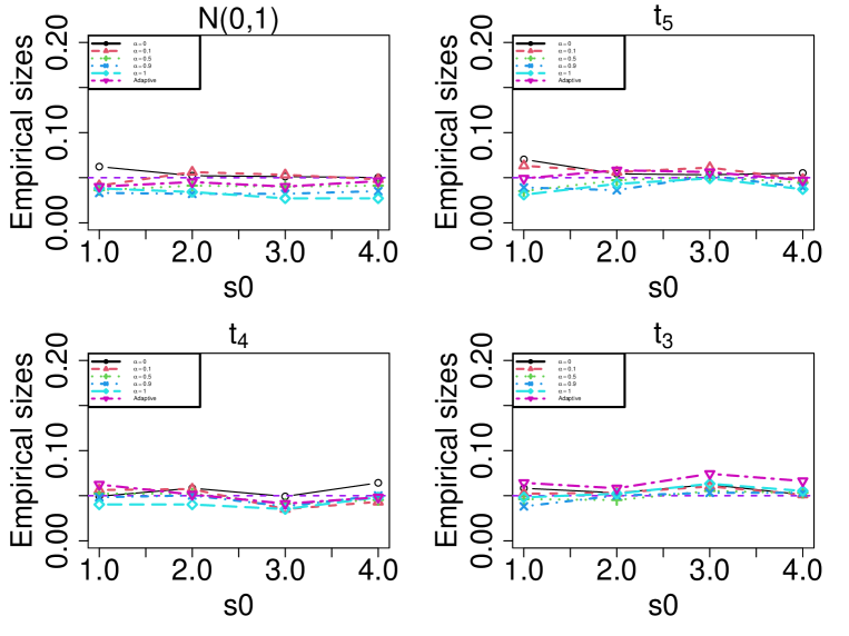
Figure 2: Empirical sizes of the individual and tail-adaptive tests for models with banded covariance matrix under the setting of $(n,p)=(200,400)$. The results are based on 1000 replications.

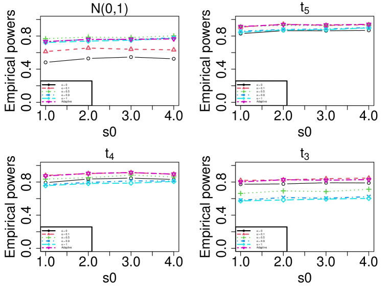
Figure 3: Empirical powers of the individual and tail-adaptive tests for models with banded covariance matrix under the setting of $(n,p)=(200,400)$. The change point is at $t_{1}=0.5$. The results are based on 1000 replications with $B=200$ for each replication.

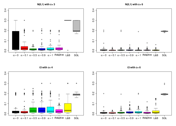
Figure 4: Boxplots of the scaled Hausdorff distance of different methods for detecting multiple change points with $(n,p)=(1000,100)$ based on 100 replications. The three change points are at $(0.25,0.5,0.75)$. L&B is the binary segmentation based technique in Leonardi and Bühlmann (2016) and SGL is the sparse graphical LASSO method in Zhang et al. (2015). The constant $c$ represents the signal strength and a larger $c$ denotes stronger signal jump.

4 Simulation Studies

We have carried out extensive numerical studies to examine the finite sample performance of our proposed new methods. To save space, we put the detailed model settings and results in Appendix A of the supplementary materials. The simulation results, including size, power and single and multiple change point estimation, can be summarized as follows:

1. As shown in Figure 2, the proposed individual and tail-adaptive tests can control the size very well under various model settings with different tail structures including both lighted and heavy tails. The individual test with $\alpha=0$ can even control the size well for Student’s $t_{2}$ and Cauchy distributions.

2. In terms of power performance, as shown in Figure 3, the individual tests perform differently under various tail structures. However, the tail-adaptive method can have powers close to its best individual one whenever the errors are lighted or heavy-tailed.

3. For single and multiple change point estimation, similar to the power analysis, the performance of the individual estimators depends on the underlying error distributions. Figure 4 indicates that the tail-adaptive estimator can perform close to its best individual estimator. Moreover, compared with the existing techniques, the tail-adaptive method enjoys better performance for single and multiple change point detection.

4. For the choice of $s_{0}$, the size performance is stable across different choices of $s_{0}$ under $\mathbf{H}_{0}$. Moreover, it is shown that, under $\mathbf{H}_{1}$, choosing $s_{0}>1$ can have high powers and accuracies than only using $s_{0}=1$ for change point testing and estimation.

In summary, the numerical results are consistent with our theorems developed in Section 3 and demonstrate the advantages of our tail-adaptive method over the existing methods.

5 Real data applications

In this section, we apply our proposed methods to the S&P 100 dataset to find multiple change points. We obtain the S$\&$P 100 index as well as the associated stocks from Yahoo! Finance (https://finance.yahoo.com/) including the largest and most established 100 companies in the S$\&$P 100. For this dataset, we collect the daily prices of 76 stocks that have remained in the S&P 100 index consistently from January 3, 2007 to December 30, 2011. This covers the recent financial crisis beginning in 2008 and some other important events, resulting in a sample size $n=1259$.

In financial marketing, it is of great interest to predict the S&P 100 index since it reveals the direction of the entire financial system. To this end, we use the daily prices of the 76 stocks to predict the S&P100 index. Specifically, let $Y_{t}\in\mathbb{R}^{1}$ be the S&P 100 index for the $t$-th day and $\bm{X}_{t}\in\mathbb{R}^{76\times 2}$ be the stock prices with lag-1 and lag-3 for the $t$-th day. Our goal is to predict $Y_{t}$ using $\bm{X}_{t}$ under the high dimensional linear regression models and detect multiple change points for the linear relationships between the S&P100 index and the 76 stocks’ prices. It is well known that the financial data are typically heavy-tailed and we have no prior-knowledge about the tail structure of the data. Hence, for this real data analysis, it seems very suitable to use our proposed tail-adaptive method. We combine our proposed tail-adaptive test with the WBS method (Fryzlewicz (2014)) to detect multiple change points, which is demonstrated in Algorithm 2. To implement this algorithm, we set $\mathcal{A}=\{0,0.1,0.5,0.9,1\}$, $s_{0}=5$, $B=100$, and $V=500$ (number of random intervals). Moreover, we consider the $L_{1}-L_{2}$ weighted loss by setting $\widetilde{\bm{\tau}}=0.5$ in (2.4). The data are scaled to have mean zeros and variance ones before the change point detection. There are 14 change points detected which are reported in Table 1.

To further justify the meaningful findings of our proposed new methods, we refer to the T-bills and ED (TED) spread, which is short for the difference between the 3-month of London Inter-Bank Offer Rate (LIBOR), and the 3-month short-term U.S. government debt (T-bills). It is well-known that TED spread is an indicator of perceived risk in the general economy and an increased TED spread during the financial crisis reflects an increase in credit risk. Figure 5 shows the plot of TED where the red dotted lines correspond to the estimated change points. We can see that during the financial crisis from 2007 to 2009, the TED spread has experienced very dramatic fluctuations and the estimated change points can capture some big changes in the TED spread. In addition, the S&P 100 index obtains its highest level during the financial crisis in October 2007 and then has a huge drop. Our method identifies October 29, 2007 as a change point. Moreover, the third detected change-point is January 10th, 2008. The National Bureau of Economic Research (NBER) identifies December of 2007 as the beginning of the great recession which is captured by our method. In addition, it is well known that affected by the 2008 financial crisis, Europe experienced a debt crisis from 2009 to 2012, with the Greek government debt crisis in October, 2009 serving as the starting point. Our method identifies October 5, 2009 as a change point after which S$\&$P 100 index began to experience a significant decline. Moreover, it is known that countries such as Italy and Spain were facing severe debt issues in July, 2011, raising fears about the stability of the Eurozone and the potential impact on global financial markets. As a result, there exists another huge drop for the S$\&$P 100 index in July 26, 2011, which can be successfully detected by our method.

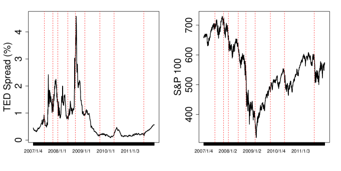
Figure 5: Plots of the Ted spread (left) and the S&P 100 index (right) with the estimated change-points (vertical lines) marked by $\#$ in Table 1.

Table 1: Multiple change poins detection for the S&P 100 dataset.

	Change points	Date	Events
	117	2007/06/21	TED Spread$\#$
	207	2007/10/29	TED Spread$\#$
	257	2008/01/10	Global Financial Crisis (TED Spread)$\#$
	360	2008/06/09	TED Spread$\#$
	439	2008/09/30	TED Spread$\#$
	535	2009/02/18	Nadir of the crisis$\#$
	632	2009/07/08
	694	2009/10/05	Greek debt crisis$\#$
	840	2010/05/05	Global stock markets fell due to fears of
			contagion of the European sovereign debt crisis$\#$
	890	2010/07/16
	992	2010/12/09
	1074	2011/04/07
	1149	2011/07/26	Spread of the European debt crisis to Spain and Italy$\#$
	1199	2011/10/05

6 Summary

In this article, we propose a general tail-adaptive approach for simultaneous change point testing and estimation for high-dimensional linear regression models. The method is based on the observation that both the conditional mean and quantile change if the regression coefficients have a change point. Built on a weighted composite loss, we propose a family of individual testing statistics with different weights to account for the unknown tail structures. Then, we combine the individual tests to construct a tail-adaptive method, which is powerful against sparse alternatives under various tail structures. In theory, for both individual and tail-adaptive tests, we propose a bootstrap procedure to approximate the limiting null distributions. With mild conditions on the regression covariates and errors, we show the optimality of our methods theoretically in terms of size and power under the high-dimensional setting with $p\gg n$. For change point estimation, for each individual method, we propose an argmax-based estimator shown to be rate optimal up to a $\log(pn)$ factor. In the presence of multiple change points, we combine our tail-adaptive approach with the WBS technique to detect multiple change points. With extensive numerical studies, our proposed methods have better performance in terms of size, power, and change point estimation than the existing methods under various model setups.

References

- Aue et al. (2009) Aue, A., Hörmann, S., Horváth, L. and Reimherr, M. (2009). Break detection in the covariance structure of multivariate time series. The Annals of Statistics 37 4046–4087.
- Bai and Perron (1998) Bai, J. and Perron, P. (1998). Estimating and testing linear models with multiple structural changes. Econometrica 66 47–78.
- Bradic et al. (2011) Bradic, J., Fan, J. and Wang, W. (2011). Penalized composite quasi-likelihood for ultrahigh dimensional variable selection. Journal of the Royal Statistical Society: Series B (Statistical Methodology) 73 325–349.
- Cho et al. (2016) Cho, H. et al. (2016). Change-point detection in panel data via double CUSUM statistic. Electronic Journal of Statistics 10 2000–2038.
- Dette et al. (2018) Dette, H., Gösmann, J. et al. (2018). Relevant change points in high dimensional time series. Electronic Journal of Statistics 12 2578–2636.
- Fryzlewicz (2014) Fryzlewicz, P. (2014). Wild binary segmentation for multiple change-point detection. The Annals of Statistics 42 2243–2281.
- Gombay and Horváth (1994) Gombay, E. and Horváth, L. (1994). Limit theorems for change in linear regression. Journal of Multivariate Analysis 48 43–69.
- Horváth (1995) Horváth, L. (1995). Detecting changes in linear regressions. Statistics 26 189–208.
- Horváth and Shao (1995) Horváth, L. and Shao, Q.-M. (1995). Limit theorems for the union-intersection test. Journal of Statistical Planning and Inference 44 133–148.
- Jiang et al. (2021) Jiang, F., Zhao, Z. and Shao, X. (2021). Modelling the covid-19 infection trajectory: A piecewise linear quantile trend model. Journal of the Royal Statistical Society: Series B (Statistical Methodology) .
- Jirak (2015) Jirak, M. (2015). Uniform change point tests in high dimension. The Annals of Statistics 43 2451–2483.
- Kaul et al. (2019) Kaul, A., Jandhyala, V. K. and Fotopoulos, S. B. (2019). An efficient two step algorithm for high dimensional change point regression models without grid search. Journal of Machine Learning Research 20 1–40.
- Koenker and Bassett Jr (1978) Koenker, R. and Bassett Jr, G. (1978). Regression quantiles. Econometrica 46 33–50.
- Lee et al. (2018) Lee, S., Liao, Y., Seo, M. H. and Shin, Y. (2018). Oracle estimation of a change point in high dimensional quantile regression. Journal of the American Statistical Association 113 1184–1194.
- Lee et al. (2011) Lee, S., Seo, M. H. and Shin, Y. (2011). Testing for threshold effects in regression models. Journal of the American Statistical Association 106 220–231.
- Lee et al. (2016) Lee, S., Seo, M. H. and Shin, Y. (2016). The lasso for high dimensional regression with a possible change point. Journal of the Royal Statistical Society: Series B (Statistical Methodology) 78 193–210.
- Leonardi and Bühlmann (2016) Leonardi, F. and Bühlmann, P. (2016). Computationally efficient change point detection for high-dimensional regression. arXiv preprint: 1601.03704 .
- Liu et al. (2020) Liu, B., Zhou, C., , Zhang, X.-S. and Liu, Y. (2020). A unified data-adaptive framework for high dimensional change point detection. Journal of the Royal Statistical Society: Series B (Statistical Methodology) 82 933–963.
- Oka and Qu (2011) Oka, T. and Qu, Z. (2011). Estimating structural changes in regression quantiles. Journal of Econometrics 162 248–267.
- Page (1955) Page, E. (1955). Control charts with warning lines. Biometrika 42 243–257.
- Pesaran and Pick (2007) Pesaran, M. H. and Pick, A. (2007). Econometric issues in the analysis of contagion. Journal of Economic Dynamics and Control 31 1245–1277.
- Qu (2008) Qu, Z. (2008). Testing for structural change in regression quantiles. Journal of Econometrics 146 170–184.
- Quandt (1958) Quandt, R. E. (1958). The estimation of the parameters of a linear regression system obeying two separate regimes. Journal of the American Statistical Association 53 873–880.
- Rinaldo et al. (2021) Rinaldo, A., Wang, D., Wen, Q., Willett, R. and Yu, Y. (2021). Localizing changes in high-dimensional regression models. In International Conference on Artificial Intelligence and Statistics. PMLR.
- Roy et al. (2017) Roy, S., Atchadé, Y. and Michailidis, G. (2017). Change point estimation in high dimensional Markov random-field models. Journal of the Royal Statistical Society: Series B (Statistical Methodology) 79 1187–1206.
- Shao and Zhang (2010) Shao, X. and Zhang, X. (2010). Testing for change points in time series. Journal of the American Statistical Association 105 1228–1240.
- Wang et al. (2021) Wang, D., Zhao, Z., Lin, K. Z. and Willett, R. (2021). Statistically and computationally efficient change point localization in regression settings. Journal of Machine Learning Research 22 1–46.
- Wang et al. (2022) Wang, X., Liu, B., Liu, Y. and Zhang, X. (2022). Efficient multiple change point detection for high-dimensional generalized linear models. The Canadian Journal of Statistics,to appear .
- Xia et al. (2018) Xia, Y., Cai, T. and Cai, T. T. (2018). Two-sample tests for high-dimensional linear regression with an application to detecting interactions. Statistica Sinica 28 63–92.
- Zhang et al. (2015) Zhang, B., Geng, J. and Lai, L. (2015). Change-point estimation in high dimensional linear regression models via sparse group Lasso. In: 53rd Annual Allerton Conference on Communication, Control, and Computing (Allerton) 815–821.
- Zhang et al. (2014) Zhang, L., Wang, H. J. and Zhu, Z. (2014). Testing for change points due to a covariate threshold in quantile regression. Statistica Sinica 1859–1877.
- Zhao et al. (2014) Zhao, T., Kolar, M. and Liu, H. (2014). A general framework for robust testing and confidence regions in high-dimensional quantile regression. Statistics .
- Zhou et al. (2018) Zhou, C., Zhou, W.-X., Zhang, X.-S. and Liu, H. (2018). A unified framework for testing high dimensional parameters: a data-adaptive approach. Preprint arXiv:1808.02648 .
- Zou and Yuan (2008) Zou, H. and Yuan, M. (2008). Composite quantile regression and the oracle model selection theory. The Annals of Statistics 36 1108–1126.