Calculation of connected contributions to the S-matrix using duality between lattice theories

Abstract

The main aim of this work - to calculate 2- and 4-point connected contributions to the $S$-matrix and correlation functions for the euclidean scalar field on the lattice with self-action $|\phi|^{n}$ for $n>2$ with coupling constant renormalised in a special way for arbitrary dimension. It is shown that the considered theory has a nontrivial continuous limit. A new method is proposed without the use of perturbation theory and diagrams. We have used the explored duality between different lattice field theories. After its application, it turns out that it is possible to apply the saddle-point method to the generating functional, where the concentration of nodes of the initial lattice approximation acts as a large parameter. In addition to the connected contributions to the $S$-matrix, the beta function is calculated. We have found a critical point for the theory of $\phi^{4k}$ in arbitrary dimension and a nontrivial mass gap of the interacting massless theory. We have received the masses of bound and single-particle states of the interacting theory. The proposed method can be extend for application to QED and gauge theories, as well as generalized to the arbitrary geometry of space. Though the way of coupling rescaling is specific, it gives nontrivial theory with the majority of perturbatively expected effects.

Calculation of connected contributions to the $S$-matrix using duality between lattice theories

1 Summary of the method and the results obtained

1.1 Description of the duality

We start with the Euclidean theory $|\phi|^{n}$ for $n>2$ with the action in arbitrary dimension $d$:

$$S[\phi]=\int_{V}d^{d}x\left(\frac{1}{2}(\nabla\phi)^{2}+\frac{m^{2}}{2}\phi^{2}+\frac{g^{n}}{n}|\phi|^{n}\right),$$ (1)

where $V$ - some finite volume (and then we also study the limit of $V\longrightarrow\infty$ and we will consider $V$ to be a cube). For even $n$, the modulus in potential can be omitted. We consider the path integral, approximating the continuous space by some lattice with a set of nodes $\{x_{k}\}_{k=1}^{N}$, which is dual by a discrete Fourier transform to the description of the system by means of a finite set of modes. For $N$ modes (equivalently, $N$ lattice nodes) action can be rewritten through the modes of the operator of the quadratic part $\hat{L}=\triangle-m^{2}$. Under the conditions, it has a real basis$\{e_{k}(x)\}$ of eigenvectors:

$$\hat{L}e_{k}=-\lambda_{k}e_{k},\qquad\lambda_{k}>0$$ (2)

Here the eigenvalues have the form:

$$\lambda_{k}=p_{k}^{2}+m^{2},$$ (3)

where $p_{k}$ - the momentum, corresponding to eigenfunction $e_{k}$. That can be explicitly written out, for example, for a cubic lattice, but for our calculation an explicit form of the lattice is not required.

We expand the fields according to the basis of eigenfunctions, and also write out a number of properties of the basis of eigenvectors:

$$\phi(x_{i})=\sum_{k=1}^{N}\phi_{k}e_{k}(x_{i}),\qquad\phi_{k}=\frac{V}{N}\sum_{i=1}^{N}\phi(x_{i})e_{k}(x_{i}),\qquad\frac{V}{N}\sum_{i=1}^{N}e_{k}(x_{i})e_{l}(x_{i})=\delta_{kl},\qquad\sum_{k=1}^{N}e_{k}(x_{i})e_{k}(x_{j})=\frac{N}{V}\delta_{ij}$$ (4)

So, $\phi_{k}$ - $k$-th the Fourier coefficient of the field $\phi(x)$, and $\phi(x_{k})$ - is the value of the field at the lattice node $x_{k}$. Then one can represent the generating functional in the form:

$$Z[j(x)]=\int\prod_{k=1}^{N}d\phi_{k}e^{-\frac{1}{2}\sum_{k=1}^{N}\lambda_{k}\phi_{k}^{2}+i\sum_{k=1}^{N}j{}_{k}\phi_{k}-\int dxV(\phi(x))}$$ (5)

We will leave the imaginary unit in front of the current for further convenience. We also introduce the concentration of lattice nodes (equivalently, the concentration of modes) by the formula $C\equiv\frac{N}{V}$. Now we can rewrite the generating functional as:

$$Z^{(N)}[j(x)]=e^{+\frac{1}{2}\sum_{k=1}^{N}\lambda_{k}\frac{\partial^{2}}{\partial j_{k}^{2}}}\prod_{k=1}^{N}\int_{\mathbb{R}}d\phi_{k}e^{+i\frac{1}{C}\sum_{k=1}^{N}j(x_{k})\phi(x_{k})-\frac{1}{C}\sum_{i=1}^{N}V(\phi(x_{i}))}$$ (6)

Let’s make a linear replacement of variables in the internal integral according to formula $(4)$, moving from the integral by modes to integration by the value of the field in the nodes:

$$Z^{(N)}[j(x)]=|\det S_{N}|\cdot e^{+\frac{1}{2}\sum_{k=1}^{N}\lambda_{k}\frac{\partial^{2}}{\partial j_{k}^{2}}}\prod_{k=1}^{N}\int_{\mathbb{R}}d\phi(x_{k})e^{+i\frac{1}{C}\sum_{k=1}^{N}j(x_{k})\phi(x_{k})-\frac{1}{C}\sum_{i=1}^{N}V(\phi(x_{i}))}$$

In this case, $\det S_{N}=\pm C^{-N/2}$, since $S_{N}\sqrt{C}$ is the transition matrix between orthonormal bases. The internal integral is the product of pointwise Fourier transforms, so it is not difficult to calculate. Next we notice that the remaining operator $e^{+\frac{1}{2}\sum_{k=1}^{N}\lambda_{k}\frac{\partial^{2}}{\partial j_{k}^{2}}}$ is the product of $N$ operators of the evolution of one-dimensional heat conduction equations, therefore its action on the function is equivalent to its convolution product with the Green’s function of the corresponding equations. This results in the following expression:

$$Z^{(N)}[j(x)]=\left(\prod_{k=1}^{N}\frac{C^{1/2}}{\sqrt{2\pi\lambda_{k}}}\right)\int\prod_{k=1}^{N}d\psi(x_{k})\exp\left[-\frac{1}{2}\sum_{k=1}^{N}\frac{(j_{k}-gC^{\frac{n-1}{n}}\psi_{k})^{2}}{\lambda_{k}}+C\int dx\cdot Ln\left[\tilde{V}\left(\psi(x)\right)\right]\right],$$

where the new potential $\tilde{V}$ determined by:

$$\tilde{V}(j)\equiv\int d\phi\cdot e^{+ij\phi-\frac{1}{n}|\phi|^{n}}$$

The functions $\psi(x)$, by which we integrate, played the role of the currents in the initial action. The graph of $-\ln|V(\psi)|$ is plotted in fig. 1.

1.2 Saddle-point computation

Since we guess to study quantum field theory, we have to make a transition to the continuous limit, which corresponds to $C\longrightarrow\infty$ and $N\longrightarrow\infty$. If we first perform a transition along $N$, remaining the concentration constant, then we will get a typical "instanton" integral, which can be calculated by the saddle-point method, but it still requires additional research. Note that so far all the transformations performed are identical, thus it is possible to develop methods for calculating $Z^{(N)}$ without rescaling the coupling constant. But for simplicity of calculations, we will consider the case when the coupling constant is rescaled in such a way that the kinetic and potential parts are equal. In this case, one can definitely get an answer using the saddle-point method. Next we will see that the theory has a nontrivial continuous limit. Thus, we rescale coupling constant as:

$$gC^{\frac{1}{2}-\frac{1}{n}}=\tilde{g}$$

Hence, we get the value:

$$Z^{(N)}[j(x)]=\left(\prod_{k=1}^{N}\frac{C^{1/2}}{\sqrt{2\pi\lambda_{k}}}\right)\int\prod_{k=1}^{N}d\psi_{k}\exp\left[-\frac{1}{2}\sum_{k=1}^{N}\frac{\tilde{g}^{2}C(j_{k}/(\tilde{g}\sqrt{C})-\psi_{k})^{2}}{\lambda_{k}}+C\int dx\cdot Ln\left[\tilde{V}\left(\psi(x)\right)\right]\right]$$

And it turns out that the value $\frac{Z^{(N)}[j(x)]}{Z^{(N)}[0]}$ has a finite limit for $C\longrightarrow\infty$ and $N\longrightarrow\infty$ (this is what we will determine as a nontrivial continuous limit).

Let’s introduce a convenient action $S^{*}[\psi]$:

$$S^{*}[\psi]=\frac{1}{2}\sum_{k=1}^{N}\frac{\tilde{g}^{2}(j_{k}/(\tilde{g}\sqrt{C})-\psi_{k})^{2}}{\lambda_{k}}+\int dx\cdot Ln\left[\tilde{V}\left(\psi(x)\right)\right]$$

We also left value of $N$ finite to avoid operations with diverges quantities. Now we also take into account the dependence of the saddle point on $j$ in higher orders, as well as the higher corrections of the saddle-point method.

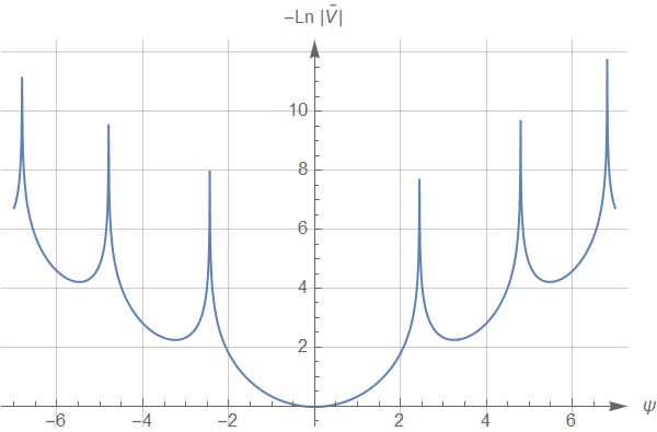
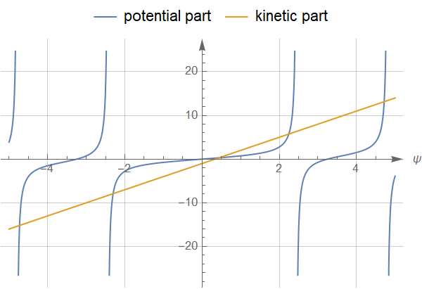
Figure 1: Plot $-Ln\ V(\eta)$ and qualitive graphs of the kinetic and potential parts of the equation $(10)$ on the extremals $S^{*}$ for the case of $N=1$

Let’s expand to the 6th order it becomes clear below why at least the 6th order is needed) the potential near zero and receive:

$$S^{*}[\psi]=\frac{1}{2}\sum_{k=1}^{N}\frac{\tilde{g}^{2}\psi_{k}^{2}}{\lambda_{k}}-\sum_{k=1}^{N}\frac{\tilde{g}\xi_{k}\psi_{k}}{\lambda_{k}}-Ln\ \tilde{V}(0)+\frac{a}{2}\int\psi^{2}(x)dx+\frac{b}{24}\int\psi^{4}(x)dx+\frac{c}{6!}\int\psi^{6}(x)dx+O(\psi^{6}),$$ (7)

where $\xi_{k}\equiv\frac{j_{k}}{\sqrt{C}}$ Here $\xi_{n}$ - small parameter, and we will expand on it. For power potentials, one can write simple explicit formulas for derivatives:

$$\tilde{V}^{(2m)}(0)=2(-1)^{m}\int_{0}^{\infty}d\phi\phi^{2m}\exp\left[-\frac{1}{n}\phi^{n}\right]=2(-1)^{m}n^{\frac{2m-n+1}{n}}\Gamma\left(\frac{2m+1}{n}\right),$$ (8)

Therefore:

$$a=n^{2/n}\frac{\Gamma(3/n)}{\Gamma(1/n)}>0,\qquad b=\frac{n^{4/n}\left(-\Gamma\left(\frac{1}{n}\right)\Gamma\left(\frac{5}{n}\right)+3\Gamma\left(\frac{3}{n}\right)^{2}\right)}{\Gamma\left(\frac{1}{n}\right)^{2}}\geq 0,$$

$$c=\frac{n^{6/n}\left(30\Gamma\left(\frac{3}{n}\right)^{3}-15\Gamma\left(\frac{1}{n}\right)\Gamma\left(\frac{5}{n}\right)\Gamma\left(\frac{3}{n}\right)+\Gamma\left(\frac{1}{n}\right)^{2}\Gamma\left(\frac{7}{n}\right)\right)}{\Gamma\left(\frac{1}{n}\right)^{3}}\geq 0$$ (9)

For any given $n$, these coefficients can be calculated explicitly. The substitution shows that for $n=2$ the coefficients $b$ and $c$ are set to zero, as it should be. Plots of dependence of coefficients $a$, $b$ and $c$ on $n$ are shown in fig. 2.

‘

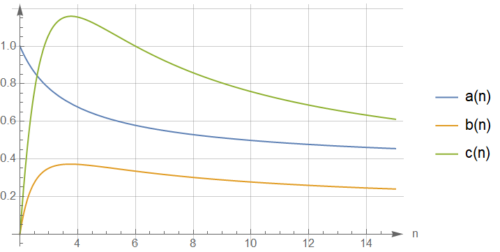
Figure 2: Plots of coefficients $a$, $b$ and $c$ depends on the degree of potential $n$

Condition of extremals ($\eta(x)$ - is the required extremal):

$$\sum_{k=1}^{N}\frac{\tilde{g}\xi_{k}}{\lambda_{k}}e_{k}(x)=\sum_{k=1}^{N}\left(\frac{\tilde{g}^{2}}{\lambda_{k}}+a\right)\eta_{k}e_{k}(x)+\frac{b}{6}\eta^{3}(x)+\frac{c}{120}\eta^{5}(x)+O(\eta^{7}),\qquad\eta(x)=\sum_{n=1}^{N}\eta_{k}e_{k}(x)$$

For $N=1$ one can easily visualise this equation. We have for this case:

$$S^{*}[\psi]=\frac{\tilde{g}^{2}(j/\tilde{g}-\psi)^{2}}{2\lambda}+Ln\left[\tilde{V}(\psi)\right],\qquad\frac{\partial S^{*}[\psi]}{\partial\psi}=-\frac{\tilde{g}^{2}(j/\tilde{g}-\psi)}{\lambda}+\frac{\tilde{V}^{\prime}(\psi)}{\tilde{V}(\psi)}$$ (10)

One can plot derivatives of kinetic and potential parts in right picture in figure 1.

It is convenient to introduce the coefficients $\theta_{k}$ using the formula:

$$\theta_{k}=\frac{1}{1+\frac{\tilde{g}^{2}}{\lambda_{k}a}},\qquad\alpha_{j}=\frac{\tilde{g}}{\lambda_{k}a}\theta_{k}$$ (11)

They are more convenient because $\theta_{k}\longrightarrow 1$ when $p_{k}\longrightarrow\infty$. Then we receive:

$$\eta_{p}(\xi)=\frac{\tilde{g}}{\lambda_{p}a}\theta_{p}\xi_{p}-\frac{b\tilde{g}^{3}}{6a^{4}}\theta_{p}\sum_{l,m,k,i}\beta_{lmi}\beta_{ikp}\frac{\theta_{l}\theta_{m}\theta_{k}}{\lambda_{l}\lambda_{m}\lambda_{k}}\xi_{l}\xi_{m}\xi_{k}+O(\xi^{5})$$ (12)

In fact, even the first term of the expansion in $\xi$ corresponds to the exact maximum of the quadratic part of the action. Therefore, for calculations up to $O(j^{5})$ we can not substitute the found cubic correction to $\eta(x)$, since it will only give an $O(j^{6})$ contribution. So, after substituting for the value of the integrand at the maximum point, we get:

$$CS^{*}[\eta(x)]+\sum_{k=1}^{\infty}\frac{j_{k}^{2}}{2\lambda_{k}}=-Ln\ \tilde{V}(0)+\sum_{k=1}^{\infty}\frac{j_{k}^{2}}{2\lambda_{k}}\frac{1}{\left(1+\frac{\tilde{g}^{2}}{a\lambda_{k}}\right)}+\frac{1}{C}\frac{b\tilde{g}^{4}}{24a^{4}}\sum_{l,q,k,p,i}\frac{\theta_{l}\theta_{q}\theta_{k}\theta_{p}}{\lambda_{l}\lambda_{q}\lambda_{k}\lambda_{p}}\beta_{qli}\beta_{ikp}j_{l}j_{q}j_{k}j_{p}+O(j^{6})$$ (13)

We see that the second order is the same as the rough calculation above.

Calcucation of the determinant gives:

$$\frac{1}{\sqrt{\det(1+\delta\tilde{S}^{\prime\prime}(\eta))}}=\exp\left[-\frac{1}{2}\frac{b\tilde{g}^{2}}{2a^{3}}\sum_{k}\frac{\theta_{k}^{2}}{\lambda_{k}^{2}}j_{k}^{2}+\frac{1}{C}\frac{\tilde{g}^{4}}{48a^{5}}\left(\frac{7b^{2}}{a}-c\right)\sum_{s,m,p,r,l}\beta_{mps}\beta_{srl}\frac{\theta_{m}\theta_{p}\theta_{r}\theta_{l}}{\lambda_{m}\lambda_{p}\lambda_{r}\lambda_{l}}j_{m}j_{p}j_{r}j_{l}+O(j^{6},1/C^{2})\right]$$ (14)

Substituting all formulas gives the result:

$$\ln\frac{Z^{(N)}[j(x)]}{Z^{(N)}[0]}=-\sum_{k=1}^{\infty}\frac{j_{k}^{2}}{2\lambda_{k}}\theta_{k}\left(1+\frac{b\tilde{g}^{2}}{2a^{3}\lambda_{k}}\theta_{k}\right)-$$

$$-\frac{1}{C}\frac{\tilde{g}^{4}}{48a^{5}}\left(c+2ab-\frac{7b^{2}}{a}\right)\sum_{s,m,p,r,l}\beta_{mps}\beta_{srl}\frac{\theta_{m}\theta_{p}\theta_{r}\theta_{l}}{\lambda_{m}\lambda_{p}\lambda_{r}\lambda_{l}}j_{m}j_{p}j_{r}j_{l}+O(j^{6},1/C^{2})$$ (15)

where, remember:

$$\theta_{k}=\frac{1}{1+\frac{\tilde{g}^{2}}{\lambda_{k}a}}$$ (16)

We also see that for a quadratic potential with $b=c=0$, the four-point function turns to $0$, as it should.

One can immediately write out two- and four-point connected correlation functions if one renormalizes the fields and vacuum so that the coefficients with $C$ go away. And then make the transition to the continuous theory without going into its details. Nevertheless, it is possible to make this transition strictly. Namely, one should connect the discrete and continuous $S$-matrices, since they are the objects that have transparent physical meaning of the probability amplitude. Then, using the reduction formula, one can obtain the relationship between the contributions to $S$-matrix in discrete and continuous theories. And only then, using the reduction formula in the opposite direction, one can get the correlators themselves in the continuous theory.

1.3 Transition from discrete to continuous theory

Although the correlators turned out to be small at high concentrations of lattice sites $C$, when substituting into the reduction formula, the scattering cross section turns out to be finite. Qualitatively, this is explained by the fact that the $in-$ and $out-$states are apparently also renormalized and the asymptotic fields contribute in $\sqrt{C}$, while $C^{-1}$ comes from the vacuum "plates" (in $1/\sqrt{C}$ from each). Therefore, as a result, the correlators turn out to be finite, and the coefficient $1/C^{k/2-1}$ is completely canceled for all correlators.

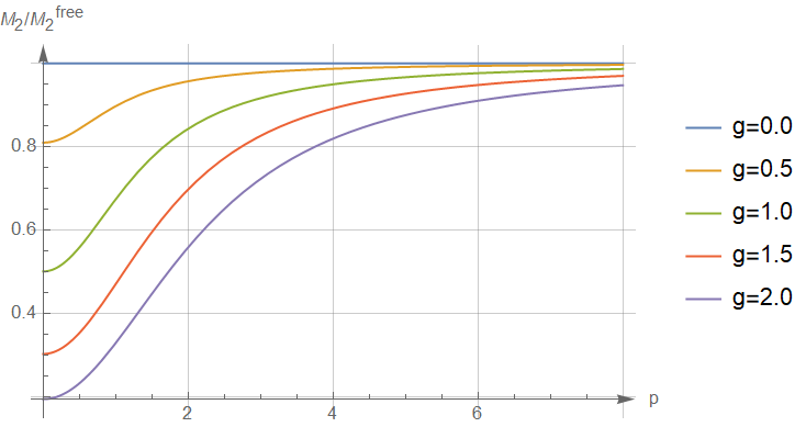
Figure 3: Qualitative plots of the prefactor in a two-point correlator $\gamma\left(p\right)=\frac{\mathcal{M}_{2}(p)}{\mathcal{M}_{2}^{free}(p)}=\frac{G_{2}(p)}{G_{2}^{free}(p)}=\theta(p)\left(1+\frac{b\tilde{g}^{2}}{2a^{3}\lambda_{p}}\theta(p)\right)$ depending on $n$ ($\tilde{g}^{2}/\lambda(p)=1$) and $p$ ($n=4$, $m=1$)

One can show that the connected contributions to the $S$-matrix in the continuous theory and its $N-$site lattice of volume $V$ approximation are related as:

$$\mathcal{M}_{c}=C^{\frac{k+l}{2}-1}\mathcal{M}_{d},$$ (17)

where $k$ is the number of incoming particles and $l$ is the number of outgoing particles. Here every $C^{1/2}$ goes from eigenfunctions normalisations, and one more $C$ is caused by the link between delta-symbol and delta-function.

As a result, we get for the two-particle $S$-matrix (two-point vertex function):

$$\mathcal{M}_{2}\left(p\right)=\lambda_{p}\theta_{p}\left(1+\frac{b\tilde{g}^{2}}{2a^{3}\lambda_{p}}\theta_{p}\right)$$ (18)

And for a connected four-particle $S$-matrix (four-point vertex function):

$$\mathcal{M}_{4}\left(q_{m},q_{s}|p_{k},p_{l}\right)=\frac{\tilde{g}^{4}}{2a^{5}}\left(c+2ab-\frac{7b^{2}}{a}\right)\theta_{m}\theta_{s}\theta_{k}\theta_{l}$$ (19)

Thus, we have obtained two- and four-particle connected contributions to the $S$-matrix for the theory $\frac{\tilde{g}^{n}}{n}|\phi|^{n}$ ($\tilde{g}$ is the rescaled constant connections) for real $n>2$ and saw that the renormalized perturbation theory indeed works for even $n>2$.

Also, the transition to infinite volume $V\longrightarrow\infty$ occurs regularly, since the dependence on the volume $V$ is found only in the values of the momenta (for a finite volume, the set of their values is discrete, and for an infinite volume, it is continuous). Therefore, the transition $V\longrightarrow\infty$ reduces simply to the change $p_{n}\mapsto p$, and we obtain for the connected two- and four-particle contributions to the $S$-matrix of the continuous theory in an infinite volume the expressions:

$$\mathcal{M}_{2}\left(p\right)=\lambda(p)\theta(p)\left(1+\frac{b\tilde{g}^{2}}{2a^{3}\lambda(p)}\theta(p)\right),\qquad\mathcal{M}_{4}\left(q,q^{\prime}|p,p^{\prime}\right)=\frac{\tilde{g}^{4}}{2a^{5}}\left(c+2ab-\frac{7b^{2}}{a}\right)\theta(p)\theta(p^{\prime})\theta(q)\theta(q^{\prime})$$

1.4 An important special case: a cube with periodic boundary conditions

After deriving formulas in a real basis, one can switch to a complex one in the final answer, since it is clearer. The constants $\beta_{ijk}$ are tensors, since they are structural constants of the associative algebra, so it is known how they are transformed. Therefore, for periodic boundary conditions and the basis of the Fourier exponents:

$$\ln\frac{Z^{(N)}[j(x)]}{Z^{(N)}[0]}=-\sum_{n=1}^{\infty}\frac{j_{k}j_{-k}}{2\lambda_{k}}\theta_{k}\left(1+\frac{1}{2}\frac{b\tilde{g}^{2}}{2a^{3}\lambda_{k}}\theta_{k}\right)-$$

$$-\frac{1}{N}\frac{\tilde{g}^{4}}{48a^{5}}\left(c+2ab-\frac{7b^{2}}{a}\right)\sum_{s,m,p,r,l}\delta_{m+p,r+l}\frac{\theta_{m}\theta_{p}\theta_{r}\theta_{l}}{\lambda_{m}\lambda_{p}\lambda_{r}\lambda_{l}}j_{m}j_{p}j_{r}j_{l}+O(j^{6},1/C^{2}),$$ (20)

where:

$$e_{k}(x)=\frac{1}{\sqrt{V}}e^{ip_{k}x},\qquad\lambda_{k}=p_{k}^{2}+m^{2},$$

and here $p^{2}$ is calculated in the Euclidean metric.

Correlators and contributions to the $S$-matrix are obtained by directly substituting the formula for $\lambda(p)$. Connected contributions to the $S$-matrix:

$$\mathcal{M}_{2}\left(p\right)=(p^{2}+m^{2})^{2}\left(\frac{1}{p^{2}+m^{2}+\tilde{g}^{2}/a}+\frac{b\tilde{g}^{2}}{2a^{3}}\frac{1}{(p^{2}+m^{2}+\tilde{g}^{2}/a)^{2}}\right),$$

and:

$$\mathcal{M}_{4}\left(q,q^{\prime}|p,p^{\prime}\right)=\frac{\tilde{g}^{4}}{2a^{5}}\left(c+2ab-\frac{7b^{2}}{a}\right)\frac{1}{1+\frac{\tilde{g}^{2}}{a(p^{2}+m^{2})}}\frac{1}{1+\frac{\tilde{g}^{2}}{a(p^{\prime 2}+m^{2})}}\frac{1}{1+\frac{\tilde{g}^{2}}{a(q^{2}+m^{2})}}\frac{1}{1+\frac{\tilde{g}^{2}}{a(q^{\prime 2}+m^{2})}}$$

1.5 Analytic continuation to other branches of the root

In the process of constructing a duality between lattice theories, we have already taken the root of the coupling constant, and we have chosen the main branch. In fact, we have $n/2$ options, and all of them correspond to some theory. And there is is another arising question which of them corresponds to the desired physics. But if we have found $Z^{(N)}[j]/Z^{(N)}[0]$ as a function $\tilde{g}$ on some open set, then it can be analytically extended to all other branches of the root in a unique way, and this continuation is carried out along all possible curves. Thus, the analytic continuation is reduced to a replacement in the resulting expressions:

$$\tilde{g}\mapsto e^{i\frac{2\pi}{n}k}\tilde{g},\qquad k=0,\dots n-1$$

But due to unitarity, the two-point correlator must be real. This means that only two branches are suitable for us:

$$\tilde{g}^{2}\mapsto\pm\tilde{g}^{2}$$

Their indices must satisfy:

$$k=\pm\frac{n}{4},\pm\frac{3n}{4}$$

That is, such branches exist only for $n\vdots 4$, in particular, for the theory $\phi^{4}$, and there are four of them. But, since we need not $\tilde{g}$, but $\tilde{g}^{2}$, only two are non-identical. Note that for $n\geq 4$ these branches, cut from the Riemann surface of the root, form a disconnected surface if the free theory $\tilde{g}=0$ is removed. That is, one can go from branch to branch only through the free theory point $\tilde{g}=0$. Therefore, in the received answers, we have to replace $\tilde{g}^{2}\mapsto\pm\tilde{g}^{2}$ for $n\vdots 4$. For such theories with respect to the coupling constant, the phase space has the form of two complex planes with cuts, glued at zero:

$$\Sigma=\left(\mathbb{C}\backslash\mathbb{R}_{<0}\right)\cup_{0\sim 0}\left(\mathbb{C}\backslash\mathbb{R}_{<0}\right)$$

For the remaining $n$ (which are not multiples of $4$) there is only one branch. We will write out the final answers and analyze them in the next section. And for them, the phase space looks like just one branch of the root:

$$\Sigma=\left(\mathbb{C}\backslash\mathbb{R}_{<0}\right)$$

2 Analysis of the obtained expressions

2.1 Limit cases

For $\tilde{g}=0$ we obtain the answer of the free theory. With $\tilde{g}\gg 1$:

$$\mathcal{M}_{2}\left(p\right)=\pm\lambda_{p}^{2}\frac{1}{\tilde{g}^{2}}\left(a+\frac{b}{2a}\right)+O\left(\frac{1}{\tilde{g}^{4}}\right),\qquad\mathcal{M}_{4}\left(q,q^{\prime}|p,p^{\prime}\right)=\frac{1}{2a}\left(c+2ab-\frac{7b^{2}}{a}\right)\frac{1}{\tilde{g}^{4}}\lambda_{p}\lambda_{p^{\prime}}\lambda_{q}\lambda_{q^{\prime}}+O\left(\frac{1}{\tilde{g}^{6}}\right)$$ (21)

Further, we will show that this dependence on the coupling constant can be easily explained qualitatively and also coincides with the already known results. As one can see, on the minus branch, the two-point correlator is negative for sufficiently large $\tilde{g}$. This can mean both that this branch is not very well defined for large $\tilde{g}$, or that when returning to coordinate time in Minkowski space, one must do a Wick rotation in the other direction for this branch.

With $\tilde{g}\ll 1$ the two-point contribution is:

$$\mathcal{M}_{2}\left(p\right)=\lambda_{p}\pm\tilde{g}^{2}\left(\frac{b}{2a^{3}}-\frac{1}{a}\right)+\frac{\tilde{g}^{4}\left(a^{2}-b\right)}{a^{4}\lambda_{p}}+O(\tilde{g}^{6})$$ (22)

And four-point:

$$\mathcal{M}_{4}\left(q,q^{\prime}|p,p^{\prime}\right)=\frac{\tilde{g}^{4}\left(-\frac{7b^{2}}{a}+2ab+c\right)}{2a^{5}}\mp\frac{\left(-\frac{7b^{2}}{a}+2ab+c\right)}{2a^{6}}\left(\frac{1}{\lambda_{p^{\prime}}}+\frac{1}{\lambda_{p}}+\frac{1}{\lambda_{q^{\prime}}}+\frac{1}{\lambda_{q}}\right)\tilde{g}^{6}+O\left(\tilde{g}^{8}\right)$$ (23)

In contrast to perturbation theory, therefore, we have an expansion not in powers of the coupling constant $G=\tilde{g}^{4}$, but in terms of the roots of this constant! This is in better agreement with the exact solution of the zero-dimensional QFT, as well as with strong coupling. As far as perturbation theory is concerned, this is a priori an asymptotic series, and it is quite expected that since it diverges, then the generating functional is probably simply not an analytic function of the coupling constant in any neighborhood of zero.

The expressions for the correlation functions are similar.

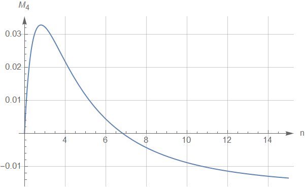
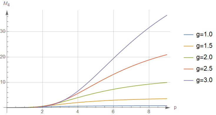
Figure 4: Qualitative plots of the four-point element of the $S$-matrix $\mathcal{M}_{4}\left(p,p|p,p\right)=\frac{\tilde{g}^{4}}{2a^{5}}\left(c+2ab-\frac{7b^{2}}{a}\right)\theta(p)^{4}$ depending on $n$ ($\tilde{g}=1$, $p=0$, $m=1$) and $p$ ($m=1$, $n=4$)

2.2 Zeros and poles

It is also interesting to look at zeros and poles of $\mathcal{M}_{2}\left(p\right)$ or $G_{2}(p)$. They are located in points:

$$\left[\begin{array}[]{cc}p^{2}=-m^{2}\\ p^{2}=-m^{2}\mp\frac{\tilde{g}^{2}}{a}\left(1+\frac{b}{2a^{2}}\right)\end{array}\right.$$ (24)

Apparently, the second zero corresponds to the presence of a second particle state in the given system, due to the presence of interaction. That is, the mass of the found "non-perturbative" particle:

$$M_{p}^{2}=m^{2}\pm\frac{\tilde{g}^{2}}{a}\left(1+\frac{b}{2a^{2}}\right)$$

As for the poles, they are located at the points:

$$p^{2}=-m^{2}\mp\frac{\tilde{g}^{2}}{a}$$ (25)

These points are the poles and $\mathcal{M}_{4}\left(q,q^{\prime}|p,p^{\prime}\right)$. Apparently, they correspond to ground states in this theory. It is also worth noting that in the presence of zero modes for the operator $\hat{L}$, our approach is also applicable, but we have to consider the operator $\hat{L}+\epsilon$ for some $\epsilon>0$ instead of $\hat{L}$ even before passing to the limit along $C,N$, and then aim $\epsilon\longrightarrow 0$ in the final answer. As a result, in the received answer, one just need to find the limit $\lambda_{k}\longrightarrow 0$ for the required $k$, then it turns out that $\theta\longrightarrow 0$, and the coefficient in the two-point function:

$$\frac{\theta(\lambda)}{\lambda}\left(1+\frac{b\tilde{g}^{2}}{2a^{3}\lambda}\theta(\lambda)\right)\longrightarrow\frac{a}{\tilde{g}^{2}}\left(1+\frac{b}{2a^{2}}\right),\qquad\lambda\longrightarrow 0$$

As a result, zero modes will have an "effective" eigenvalue $\lambda_{0}^{*}=\frac{\tilde{g}^{2}}{a}\left(1+\frac{b}{2a^{2}}\right)^{-1}$ caused by the presence of an interaction. For $\tilde{g}\longrightarrow 0$, as we see, we receive a zero mass gap, as it should be in a noninteracting theory. Thus, the described approach predicts the presence of a nonzero mass gap even for an initially massless theory. It is noteworthy that this answer does not depend on the geometry of space. which indicates the existence of a non-zero mass gap for a massless theory in any space-time geometry. Its width is thus:

$$\Delta m^{2}=\pm\frac{\tilde{g}^{2}}{a}\left(1+\frac{b}{2a^{2}}\right)^{-1}$$

That is, the first branch has a non-trivial mass gap, while the second does not.

As for critical points, then for them the following should be performed:

$$m^{2}\pm\frac{\tilde{g}^{2}}{a}=0$$

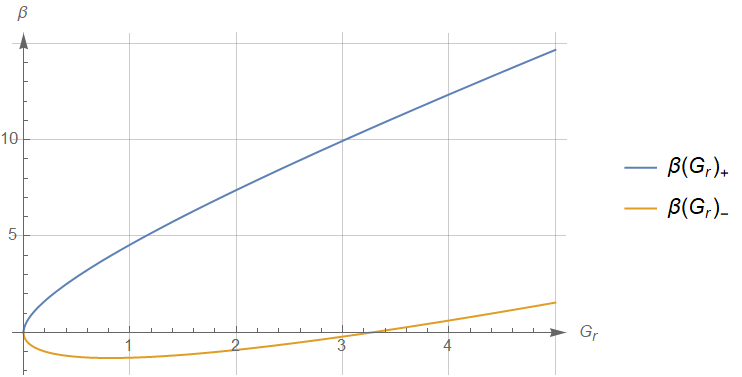
Figure 5: Plots of beta functions for the received answer for $m_{r}=3$

That is, there is no critical point on the first branch (we consider $m^{2}>0$ in our consideration), but there is on the second. In principle, there is nothing surprising in this, since, apparently, the phase space of the considered family of theories is parametrized not $\tilde{g}^{n}$, but $\tilde{g}^{2}$, that is, it represents a Riemann surface for the coupling constant root. And we just got the statement on which branch of the root the critical point is localized (when it exists).

It is interesting to note that two branches were also obtained in Suslov (2008) by resumming the perturbation series, which we briefly discuss in subsection 3.3.

That is, for $n\vdots 4$ the critical point exists in all dimensions, but for the remaining $n>2$ it does not exist.

3 Comparison with already known results

3.1 Strong coupling approximation, general structure

In fact, the calculations we performed are very similar to the work of Bender et al. (1979), with the exception that the authors of this work stopped even before rewriting the action through the kernel of the heat equation, and after calculating the Fourier transforms, they began to expand into series. Next, the authors study how to rescale the coupling constant to obtain a non-trivial continuous limit. So, the authors rescaled coupling constant after strong expansion, whereas in this work the rescaling was done in path integral. This is the main reason of mismatching of coefficients in strong-coupling of the expansion, though the amalytical structure is the same/

Namely, the authors constructed a strong coupling expansion for the theory $g^{4}\phi^{4}/4$ and proposed a diagram technique for calculating the coefficients $C_{k}$:

$$\ln Z[j]=C_{0}+\sum_{k=1}^{\infty}g^{-2k}C_{k}[j],$$

s use $\delta(0)$ - ultraviolet clipping theory, and a constant:

$$R=\Gamma(3/4)/\Gamma(1/4)$$

The constant $\delta(0)$ in author’s notations is nothing but the concentration $C^{1/2}$. For convenience of comparison, we immediately rewrite using $C=\delta(0)$, $\tilde{g}^{2}=C^{1/4}g^{2}$. Then the ratio of generating functionals has the form:

$$\ln\frac{Z[j]}{Z[0]}=\sum_{k=1}^{\infty}g^{-2k}(C_{k}[j]-C_{k}[0])=-\frac{R}{\tilde{g}^{2}}\int dxj(x)^{2}+$$

$$+\frac{R^{2}}{\tilde{g}^{4}}2\iint dxdyj(x)G^{-1}(x,y)j(y)+\left(\frac{1}{24}-\frac{1}{2}R^{2}\right)\frac{1}{C\tilde{g}^{4}}\int dx\left[j(x)^{4}+6G^{-1}(x,x)j(x)^{2}\right]+\dots$$

The first thing that one can notice is the coincidence of the expansion degrees in $\tilde{g}$ in the strong coupling series. The second is the external similarity of the coefficients. Using the properties of the gamma function, we can express them in terms of $R$:

$$a=2R\qquad b=12R^{2}-1,\qquad c=24R(10R^{2}-1)$$

Next, the authors try to pass to the continuous limit by considering various cases of redefining the coupling constant, comparing with some results of numerical simulations. If, however, we fix $\tilde{g}$ as a constant, as was done in this paper, then in the limit of the continuous theory $N,C\longrightarrow\infty$ we obtain the same powers of $C$ for correlators of given orders as in the decomposition obtained. If we rewrite the obtained answer in terms of modes in some real orthonormal basis, we get after simplifications:

$$\ln\frac{Z[j]}{Z[0]}=-\frac{1}{\tilde{g}^{2}}\sum_{k=1}^{N}j_{k}^{2}\left(R+\left(\frac{1}{4}-R^{2}\right)\frac{\lambda_{k}}{\tilde{g}^{2}}\right)+\left(\frac{1}{24}-\frac{1}{2}R^{2}\right)\frac{1}{C\tilde{g}^{4}}\sum_{k,l,m,i,s}\beta_{mks}\beta_{sli}j_{m}j_{k}j_{l}j_{i}+\dots$$

On the other hand, the strong coupling expansion $\tilde{g}\gg 1$ for the result obtained in this work:

$$\ln\frac{Z^{(N)}[j(x)]}{Z^{(N)}[0]}=-\frac{1}{2\tilde{g}^{2}}\sum_{k=1}^{\infty}j_{k}^{2}\left(\left(a+\frac{b}{2a}\right)-\left(a^{2}+b\right)\frac{\lambda_{k}}{\tilde{g}^{2}}\right)-$$

$$-\frac{1}{C}\frac{1}{48a}\left(c+2ab-\frac{7b^{2}}{a}\right)\frac{1}{\tilde{g}^{4}}\sum_{s,m,p,r,l}\beta_{mps}\beta_{srl}j_{m}j_{p}j_{r}j_{l}+O(j^{6},1/C^{2})$$

As we can see, the coefficients do not coincide with the expansion obtained by the authors, although the analytical structure is the same. Apparently, the point is that we are still considering a theory with a coupling constant rescaled in a special way, which is not a pure $|\phi|^{n}$.

As for arbitrary powers $n$ of the potential $|\phi|^{n}$, as shown in the same article, one obtains an expansion in powers of $g^{-k/n}$, where $k\in\mathbb{N}_{0}$, as and in this work.

3.2 Beta function and Wilson renormalization group

3.2.1 One-loop result

We will use the ready-made results for one-loop beta functions for different dimensions $d$, obtained, for instance, in Vereijken (2017) The renormalized action of the form ($k$ - is the cutoff parameter) was considered there:

$$S_{k}[\phi]=\int d^{d}x\left[-\frac{1}{2}z_{k}\phi(x)\partial_{x}^{2}\phi(x)+\frac{1}{2}m_{k}^{2}\phi(x)^{2}+\frac{G_{k}}{4}\phi(x)^{4}\right]$$ (26)

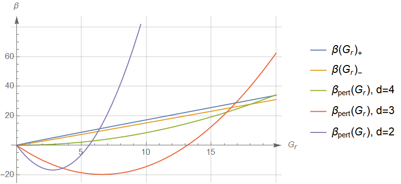
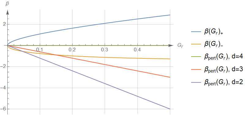
Figure 6: Comparison of graphs of the beta function for our calculated answer $\beta(G_{r})$ with perturbative one-loop calculations in different dimensions. Left and right - different ranges of values of the coupling constant. The abscissa shows the values of the renormalized coupling constant. The renormalized mass is given here: $m_{r}=3$

Using the functional renormalization group as in Wetterich (1993), ine can get the following well-known expression for one-loop beta-function:

$$\beta_{pert}(m_{r}^{2},G_{r})=\beta_{G_{r}}(z_{k}=1)=\frac{6^{3}G_{r}^{2}}{2^{d}\pi^{d/2}\Gamma\left(\frac{d}{2}+1\right)\left(1+m_{r}^{2}\right)^{3}}-(4-d)G_{r},$$ (27)

where, for brevity of notation, we have begun to omit the index $k$ of the renormalized parameters.

3.2.2 The exact value of the beta function for the calculation done

Main root branch

Everywhere, when comparing beta functions, we will assume $n=4$, since only for $\phi^{4}$ we have calculated the vertex function corresponding to the renormalized coupling constant, for higher degrees we need to consider higher orders of correlators.

Let us now calculate the beta function of the main branch as the root of the answer we received. Let’s start by fixing the renormalization scheme:

$$\mathcal{M}_{2}(p=im_{r})=0,\qquad\frac{d\mathcal{M}_{2}(p^{2}=-\mu^{2})}{d(p^{2})}=1,\qquad G_{r}=\mathcal{M}_{4}\bigg{|}_{p_{i}^{2}=-\mu^{2}}=\frac{\tilde{g}^{4}}{2a^{5}}\left(c+2ab-\frac{7b^{2}}{a}\right)\theta(p^{2}=-\mu^{2})^{4}$$ (28)

As a result, the expression for the beta function takes the form:

$$\beta(m_{r},G_{r})=\frac{8\left(a^{2}-b\right)\left(a+b-a^{2}\right)}{ab}G_{r}+\frac{8a^{3}\alpha^{2}m_{r}^{2}\left(a^{2}-b\right)^{2}}{b^{3}}\sqrt{G_{r}}$$ (29)

That is, it has a qualitative appearance:

$$\beta(m_{r},G_{r})=AG_{r}+Bm_{r}^{2}G_{r}^{1/2},\qquad A,B>0,\qquad A\approx 1.62094,\qquad B\approx 0.325763$$ (30)

for $A,B$ - constant coefficients. As we can see, on the main branch there are no critical points, which is consistent with the earlier analysis of two-point correlation functions.

Analytical continuation to the remaining branches of the root

As we have already understood from subsection 1.5, only two branches can potentially be physical: the main one and the opposite one, when $\tilde{g}^{2}$ is replaced by $-\tilde{g}^{2}$. Accordingly, we have to replace:

$$G_{r}^{1/2}\mapsto-G_{r}^{1/2}$$

That is, we can immediately write down a ready-made answer for the beta function:

$$\beta(m_{r},G_{r})=AG_{r}-Bm_{r}^{2}G_{r}^{1/2},\qquad A,B>0,\qquad A\approx 1.62094,\qquad B\approx 0.325763$$

With the same coefficients $A$ and $B$ as for the first branch. For this branch, as we can see, there is already a zero of the beta function, and it is located at:

$$G_{r}=\frac{B^{2}}{A^{2}}m_{r}^{4}$$

Again, we obtain by agreement with the analysis of the received answers without using the renormalization group, since we already obtained earlier that there is a critical point on the second branch.

It is worth noting that our result predicts the presence of a critical point for $\phi^{4}$ in any dimensions on the second branch.

3.2.3 Comparison of the obtained result with the perturbative one

Now we can plot the perturbative and obtained results (for both branches) on the same graph, setting, for example, the renormalized mass $m_{r}=3$ (this is the most convenient value for comparitive plot). For masses of the order of unity, the qualitative picture will not change, as is easy to see.

The qualitative form of the obtained beta function coincides with the perturbative one-loop results. As for the quantitative coincidence, it is observed only for sufficiently small $G_{r}\sim 0.1$. However, the conclusions of perturbation theory are valid only for sufficiently small coupling constants. For the dimensions $d\geq 5$ the agreement is worse, which can be easily explained by the fact that for these dimensions the theory stop to be renormalizable. Also, the coincidence worsens for too large and too small renormalized masses $m_{r}$.

3.3 Strong coupling limit

Let us now compare our result with the calculation in the strong coupling limit of the result in Suslov (2008), obtained by resumming the series of perturbation theory and instanton contributions. Namely, it was found that in a space of dimension $d$ (depending on the choice of the sheet of analytic continuation):

$$\beta(G_{r})=\left[\begin{array}[]{cc}d\cdot G_{r},\\ (d-4)\cdot G_{r}\end{array}\right.$$

As one can see, our values are pretty close to the first sheet for $d\approx 2,3,4$. And for large $d$, the theory $\phi^{4}$ is no longer renormalizable, so there is no special point in comparing it with perturbation theory. In general, a comparison with various results for $d=4$ is shown in the graph below (for massless cases, since this is the situation most often considered by various authors). Thus, there is a fairly good agreement with the results of the resummed perturbation theory. It is also interesting that here, too, two branches of theories are obtained for a given value of $G_{r}$, as in our result.

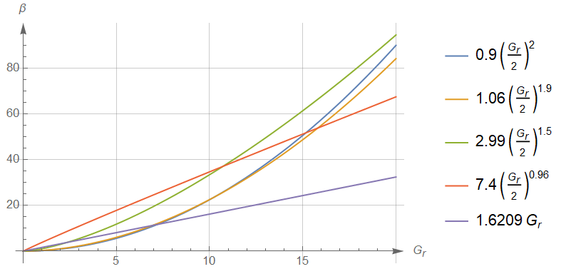
Figure 7: Comparison with various results for $d=4$ for massless theories (Suslov (2010, 2008); Kazakov et al. (1979); Kubyshin (1984); Sissakian et al. (1994)). Our chart is the purple line

4 Discussion of results and directions for further research

In this paper, we propose a method for calculating the generating functional in quantum field theory and obtain the first two vertex functions (for two and four particles) for the case of a specially rescaled coupling constant. The answer is very similar in form to the predictions of the renormalized perturbation theory, but everything can be expressed in terms of the bare Lagrangian parameters. A qualitative agreement was obtained between the beta functions and the existing calculations for strong and weak coupling. We also obtained a qualitative agreement between the vertex functions and the known expansion results in the strong coupling model.

The advantages of the proposed method are:

1. Its comparative simplicity and transparency

2. The ability to write the final answer explicitly

3. Good qualitive agreement with the already available results (renormalized perturbation theory and strong coupling expansions)

4. Possibility of generalisation for theories without scaled parameters

Nevertheless, it is reasonable to present a number of questions to this calculation, including:

1. No dependence on the dimension of space

2. Specific "rescale" of the coupling constant in the Lagrangian $gC^{\frac{1}{2}-\frac{1}{n}}=\tilde{g}=const$ and dependence of the result on rescaling

3. Correctness of the approximation of the continuous theory of the discrete one (definition of the path integral)

4. The smallness of errors in the "infinite-dimensional" saddle-point method

The first point is partly related to the fact that after applying the described duality, we pass from a local QFT to a nonlocal QFT with an integral operator of a good function in the quadratic part. And, as is known Efimov (1970), the dependence of such theories on the dimension of space is really quite weak. Perhaps, in order to take into account the dimension of space, it is necessary to take a closer look at the first transition, and it is possible that small $k$ and, edge effects caused by the finiteness of $V$, will play a role. Also, perhaps, the whole point is in rescaling $g$.

The second point is dictated by the desired simplicity of the calculation. However, the value of this study is that we offer a method that can be improved and extended, because after applying duality, we get an integral with a large parameter.

From the predictions being checked, we have obtained that for the case $gC^{\frac{1}{2}-\frac{1}{n}}=\tilde{g}=const$:

1. The theory $\phi^{4k}$ must have a critical point for any space dimension, while the theories $|\phi|^{n}$ have no critical points for all other $n>2$

2. For all $n$, on the “positive” branch $+\tilde{g}^{2}$ there exists a non-trivial mass gap $\Delta m^{2}=\frac{\tilde{g}^{2}}{a}\left(1+\frac{b}{2a^{2}}\right)^{-1}$ for massless theory

3. For $n\geq 6.8$, the theories $|\phi|^{n}/n$ must have a four-point function that is negative (that is, repulsive at an initially attractive potential)

4. $\phi^{n}/n$ seems to exist $(\pm$ corresponds to the case $n\vdots 4$, the sign is chosen depending on the branch; for all other $n>2$ only the upper sign takes place):

   1. Bound state with mass squared $M_{c}^{2}=m^{2}\pm\frac{\tilde{g}^{2}}{a}$

   2. One-particle state with squared mass $M_{p}^{2}=m^{2}\pm\frac{\tilde{g}^{2}}{a}\left(1+\frac{b}{2a^{2}}\right)$ (besides the "trivial" asymptotic state of mass $m$)

As for point $2$, it cannot be verified by methods of perturbation theory, since these theories are not renormalizable in $d\neq 1,2,3$. It would be interesting to find some physical effect that confirms or refutes this statement. As for point $1$, as far as we know, there is no adequate proof of the absence of a critical point at $d=4$ for $\phi^{4}$, and the multiloop calculation of the beta function says nothing, since the signs in it alternate, and formally one can it would be to look for zero at the beta function, as it is customary to do. In addition, in Baker and Kincaid (1979) $\phi^{4}$ in dimension $d=4$ was investigated, and the authors argue that the existence of another fixed point is very plausible, but its nature and area of attraction are unclear.

Concluding, although we considered a special way of coupling rescaling for the simplicity of calculations, it gives a rise to a nontrivial theory with the majority of perturbatively expected phenomena. Described theory represents strong coupling well, but it lacks of some kind of phase transition. This phase transition means the end of the zone where strong coupling expansion works and the start of the zone where perturbation theory works.

Appendix. Properties of beta constants

By beta constants we mean the structure constants of the (associative) eigenfunction algebra $\hat{L}$ with respect to pointwise multiplication. That is:

$$e_{n}(x)\cdot e_{m}(x)=\sum_{k}\beta_{nmk}e_{k}(x)$$ (31)

It can also be written that (since the basis is orthonormal):

$$\beta_{nmk}=<e_{n}(x)\cdot e_{m}(x),e_{k}(x)>$$

Associativity implies that:

$$\sum_{i}\beta_{nmi}\beta_{ikl}=\sum_{i}\beta_{nki}\beta_{iml}$$ (32)

Also, $\beta_{nmk}$ are symmetrical in the first two indices. For a real orthonormal basis, $\beta_{nmk}$ are symmetric in all three indices. $\beta$ constants are a convenient formalism for working with sums over modes, and, in principle, all the same results can be obtained in the coordinate version using the properties of orthogonality and completeness of the basis of eigenfunctions.

We are mainly interested in the cases where $\hat{L}=\triangle-m^{2}$ on a cube $X\subset\mathbb{R}^{n}$ of unit volume with periodic and zero boundary conditions. In both cases, $e_{n}(x)$ are easily found and are the basis for the entire $L^{2}(X)$, namely:

1. $e_{m}(x)=e^{ip_{m}x}$ (in the sense of the dot product), $\overrightarrow{p}_{m}=2\pi\overrightarrow{m}$, $\overrightarrow{m}\in\mathbb{Z}^{n}$, $\beta_{nmk}=\delta_{n+m,k}$ (in the sense of vector indices) for periodic conditions

2. $e_{m}(x)=2^{n/2}\sin(p_{m}^{1}x_{1})\cdot...\cdot\sin(p_{m}^{n}x_{n})$, $\overrightarrow{p}_{m}=2\pi\overrightarrow{m}$, $\overrightarrow{m}\in\mathbb{Z}^{n}$, for null conditions ($\beta_{nmk}$ has a slightly more complex form, but it counts)

Let us prove several useful properties (Whole $\beta$ depends on $C$, but we do not write index $C$ for brevity).

Proposition.

$\sum_{i,n,l}\beta_{mni}\beta_{ikl}\beta_{nlp}=C\beta_{mkp}$

Proof.

$N\sum_{p}\beta_{mkp}e_{p}(x)=\sum_{i}e_{m}(x)e_{k}(x)e_{i}(x)^{2}=\sum_{i}e_{m}(x)e_{i}(x)\cdot e_{k}(x)e_{i}(x)=\sum_{i,n,l}\beta_{mni}\beta_{ikl}\beta_{nlp}e_{p}(x)$, hence the written statement follows. ∎

Proposition.

$\sum_{i,k}\beta_{mik}\beta_{ikn}=C\delta_{nm}$

Proof.

$Ce_{m}(x)=\sum_{i}e_{m}(x)e_{i}(x)e_{i}(x)=\sum_{i}\beta_{mik}\beta_{kil}e_{l}(x)$, hence the written statement follows. ∎

Also note that for complex exponents (periodic conditions):

$$\sum_{s}\beta_{mps}\beta_{s\mu\nu}=\delta_{m+p,\mu+\nu},$$

As for the convolutions of two beta tensors with respect to the same index, one can verify by the example of the basis of sines and cosines for a cube with periodic boundary conditions, the sum:

$$\sum_{s}\beta_{mps}\beta_{s\mu\nu}\sim\delta_{m+p,\mu+\nu},$$

or the sum of similar delta-characters. A similar situation will be with the basis of sines for a cube with zero boundary conditions. Therefore, a new degree $C$ will not arise from there, in contrast to the higher-order convolutions discussed above.

References

- Suslov [2008] I. M. Suslov. Analytical asymptotics of -function in theory (end of the "zero charge" story), 2008. URL https://arxiv.org/abs/0804.0368.
- Bender et al. [1979] Carl Bender, Fred Cooper, G. Guralnik, and David Sharp. Strong-coupling expansion in quantum field theory. Physical Review D, 19:1865–1881, 03 1979. doi:10.1103/PhysRevD.19.1865.
- Vereijken [2017] Arthur Vereijken. Functional renormalization group for scalar field theories. Radpoud Universiteit Nijmegen, 2017.
- Wetterich [1993] Christof Wetterich. Exact evolution equation for the effective potential. Physics Letters B, 301(1):90–94, feb 1993. doi:10.1016/0370-2693(93)90726-x. URL https://doi.org/10.1016%2F0370-2693%2893%2990726-x.
- Suslov [2010] I.M. Suslov. Strong coupling asymptotics of the -function in theory and qed. Applied Numerical Mathematics, 60(12):1418–1428, 2010. ISSN 0168-9274. doi:https://doi.org/10.1016/j.apnum.2010.05.006. URL https://www.sciencedirect.com/science/article/pii/S0168927410000851. Approximation and extrapolation of convergent and divergent sequences and series (CIRM, Luminy - France, 2009).
- Kazakov et al. [1979] D. I. Kazakov, D. V. Shirkov, and O. V. Tarasov. Analytical Continuation of Perturbative Results of the Model Into the Region Is Greater Than or Equal to 1. Theor. Math. Phys., 38:9–16, 1979. doi:10.1007/BF01030252.
- Kubyshin [1984] Yu. A. Kubyshin. Sommerfeld-watson summation of perturbation series. Theoretical and Mathematical Physics, 58:91–97, 1984.
- Sissakian et al. [1994] A.N. Sissakian, I.L. Solovtsov, and O.P. Solovtsova. -function for the -model in variational perturbation theory. Physics Letters B, 321(4):381–384, 1994. ISSN 0370-2693. doi:https://doi.org/10.1016/0370-2693(94)90262-3. URL https://www.sciencedirect.com/science/article/pii/0370269394902623.
- Efimov [1970] G. V. Efimov. Nonlocal quantum field theory, nonlinear interaction lagrangians, and the convergence of the perturbation-theory series. Theoretical and Mathematical Physics, 1970. URL https://doi.org/10.1007/BF01038039.
- Baker and Kincaid [1979] George A. Baker and John M. Kincaid. Continuous-spin ising model and field theory. Phys. Rev. Lett., 42:1431–1434, May 1979. doi:10.1103/PhysRevLett.42.1431. URL https://link.aps.org/doi/10.1103/PhysRevLett.42.1431.
- Suslov [2001] I. M. Suslov. Summing divergent perturbative series in a strong coupling limit. the gell-mann-low function of the theory. Journal of Experimental and Theoretical Physics, 93(1):1–23, jul 2001. doi:10.1134/1.1391515. URL https://doi.org/10.1134%2F1.1391515.
- Wilson [1983] Kenneth G. Wilson. The renormalization group and critical phenomena. Rev. Mod. Phys., 55:583–600, Jul 1983. doi:10.1103/RevModPhys.55.583. URL https://link.aps.org/doi/10.1103/RevModPhys.55.583.
- Fedoruk [2015] M. V. Fedoruk. Saddle point method. URSS, 1 edition, 2015.