Quantum third-order nonlinear Hall effect of a four-terminal device with time-reversal symmetry

Abstract

The third-order nonlinear Hall effect induced by Berry-connection polarizability tensor has been observed in Weyl semimetals T_d-MoTe₂ as well as T_d-TaIrTe₄. The experiments were performed on bulk samples, and the results were interpreted with the semiclassical Boltzmann approach. Beyond the bulk limit, we develop a quantum nonlinear transport theory to investigate the third-order Hall response of a four-terminal setup with time-reversal symmetry in quantum regime. The quantum nonlinear theory is verified on a model system of monolayer MoTe₂, and numerical results on the angle-resolved Hall currents are qualitatively consistent with the experiment. More importantly, quantum signatures of the third-order Hall effect are revealed, which are independent of the system symmetry. The first quantum signature is quantum enhancement of the third-order Hall current, which is characterized by sharp current peaks whose magnitudes are three orders larger than the first-order Hall current. Such quantum enhancement originates from quantum interference in coherent transport, and it can be easily destroyed by dephasing effect. The second quantum signature is disorder-induced enhancement of the third-order Hall current for weak disorders. Our findings reveal quantum characteristics of the third-order Hall effect, and we propose feasible ways to enhance it in nanoscale systems. The quantum third-order theory developed in this work provides a general formalism for describing nonlinear coherent transport properties in multi-terminal devices, regardless of the system symmetry.

I Introduction

Berry curvature related nonlinear Hall responses in time-reversal invariant systems have attracted intensive research interest in condensed matter physics as well as material science. The second-order Hall effect induced by Berry curvature dipole (BCD) has been thoroughly studied both theoreticallyL-Fu1 ; Guinea1 ; NHEREV ; Lee ; Ortix ; Sodemann ; Tsymbal and experimentally in various aspectsS-Xu ; Q-Ma ; K-Kang ; J-Xiao ; H-Yang . Meanwhile, the third-order Hall effect induced by Berry-connection polarizability tensor (BPT), another band geometric quantityGao14 ; Gao15 ; Gao17 ; syyang21 , was experimentally realized in thick micron-sized T_d-MoTe₂ samples in 2021THE2021 , where the third-order Hall current depends on the relaxation time and hence it is an extrinsic Hall effect. Very recently, room temperature third-order Hall effect was observed in bulk Weyl semimetal TaIrTe₄ with thickness of 160 $nm$, which can stably exist for several monthsTHE2022NSR . On the theoretical aspect, BPT-induced third-order Hall effect was predicted in multi-Weyl semimetals through model calculationNLHE2021AN and monolayer FeSe with first-principles calculationTHE2022 . If the time-reversal symmetry is broken, it was proposed that the third-order nonlinear anomalous Hall effect can be caused by Berry curvature quadruples in certain antiferromagnets such as monolayer SrMnBi₂KTLAW2021 .

Up to now, the third-order Hall effect with time-reversal symmetry was experimentally performed on bulk samplesTHE2021 ; THE2022NSR to observe optimized nonlinear response signals. Related theoretical interpretations were based on the second-order semiclassical approachGao14 for bulk systems, where the field-induced Berry connection and BPT play crucial roles on the extrinsic third-order Hall effectTHE2021 ; NLHE2021AN ; THE2022NSR . Quantum characteristics of the third-order Hall effect in nanoscale systems has not been addressed. In nanoscale devices, quantum coherent transport is dominant. Therefore, a real-space quantum nonlinear theory is necessary to simulate the third-order Hall response of multi-terminal systems in quantum regime and compare with the second-order semiclassical approach, which is absent so far.

To fill in this gap, we develop a quantum nonlinear transport theory to numerically investigate the third-order Hall response of multi-terminal devices in the presence of time-reversal symmetry. This gauge-invariant quantum nonlinear theory allows direct calculation of the third-order conductances, rather than the semiclassical conductivity. We apply this theory to a 2-dimensional (2D) massive Dirac model describing monolayer T_d-MoTe₂, and calculate angular-dependent Hall currents (from first order to third order) of a four-terminal Hall setup via rotating four perpendicular leads. The numerical results are qualitatively consistent with both the experiment and the semiclassical approach in Ref.[THE2021, ]. More importantly, in quantum regime, the third-order Hall current can be enhanced to three orders of magnitude larger than the first-order Hall current, which was only one order of magnitude in the bulk systemTHE2021 . Experimentally observed third-order Hall signals in bulk systems are relatively weak, where the typical third-order Hall voltage is in the order of $\mu V$ in response to a driving voltage in the order of 10 $mV$THE2021 ; THE2022NSR . Therefore, enhanced third-order Hall signal is expected in quantum regime. Such quantum enhancement of the third-order Hall current is attributed to the quantum interference in coherent transport, which is verified by introducing phase relaxation process that severely reduces the sharp current peaks. We also observe disorder-induced enhancement of the third-order Hall effect, where similar disorder effect has been predicted in BCD-induced second-order Hall effectdisorderNHE ; QTNHE . These findings highlight quantum characteristics of the third-order Hall effect, which can be experimentally studied in nanoscale Weyl semimetals T_d-MoTe₂ and T_d-TaIrTe₄, etc.

The rest of the paper is organized as follows. In Sec. II, a gauge-invariant quantum third-order transport theory is derived. The quantum nonlinear theory is applied to a four-terminal device with time-reversal symmetry, and numerical results are presented in Sec. III. A summary is finally given in Sec. IV.

II Quantum third-order nonlinear transport theory

We start from the Landauer-Büttiker formula describing quantum transport ($\hbar=e=1$)

$$I_{\alpha}=\sum_{\beta}\int_{E}{\rm Tr}[A_{\alpha\beta}]f_{\beta},$$ (1)

where $A_{\alpha\beta}=\Gamma_{\alpha}G^{r}\Gamma_{\alpha\beta}G^{a}$, $\Gamma_{\alpha\beta}=\Gamma_{\beta}-\delta_{\alpha\beta}\Gamma$, and $\Gamma=\sum_{\alpha}\Gamma_{\alpha}$. $G^{r}(G^{a})$ is the retarded(advanced) Green’s function. $\Gamma_{\alpha}$ is the linewidth function of probe $\alpha$ characterizing the coupling between this probe and the scattering region. $f_{\beta}=f_{\beta}(E+v_{\beta})$ is the Fermi distribution function of probe $\beta$, and $v_{\beta}$ is the bias voltage in this probe.

One of the fundamental requirements for quantum transport is the gauge-invariant conditionbut01 ; but02 , i.e., the current remains unchanged when the bias voltage in each probe changes by a constant amount. In quantum transport, one has to consider the self-consistent Coulomb interaction to satisfy gauge invariance. This Coulomb potential is due to the charge injection and hence it is a nonequilibrium potential which vanishes at zero biasbut01 ; but02 . We use a two-probe system to illustrate the importance of gauge invariance. From Eq.(1), the current $I_{L}$ from the left probe to the second order in bias voltage is expressed as

$$I_{L}=G_{11}(v_{L}-v_{R})+G_{111}(v_{L}^{2}-v_{R}^{2})+...$$ (2)

For $v_{L}=v$ and $v_{R}=0$, the current is $I_{L}=G_{11}v+G_{111}v^{2}$; while for $v_{L}=0$ and $v_{R}=-v$, the current is $I_{L}=G_{11}v-G_{111}v^{2}$, which is clearly gauge dependent and the result is qualitatively incorrect. Therefore, it is essential to have a gauge-invariant formalism in order to obtain reliable results. The gauge-invariant theory of the second-order conductance has been developed long agobut1 ; ma ; baigen . In this work, we develop the quantum third-order transport theory.

To investigate the nonlinear conductance, it is convenient to work within the nonequilibrium Green’s function formalism (NEGF). In this formalism, the Hamiltonian of the scattering region contains a self-consistent Coulomb potential and hence the retarded Green’s function is written as

$$G^{r}(E)=\frac{1}{E-H-qU-\Sigma^{r}},$$ (3)

where the self-consistent Coulomb potential satisfies the Poisson equation

$$\nabla^{2}U(x)=4\pi qi\int_{E}G^{<}(E,x,x).$$ (4)

The lesser Green’s function is $G^{<}=iG^{r}\sum_{\alpha}\Gamma_{\alpha}f_{\alpha}G^{a}$. $\Sigma^{r}=\sum_{\alpha}\Sigma^{r}_{\alpha}(E-qv_{\alpha})$ is the self-energy due to the probesbaigen .

When expanding the current in Eq.(1) to the third order under the condition of small bias voltages, we have

$$I_{\alpha} = G_{\alpha\beta}v_{\beta}+G_{\alpha\beta\gamma}v_{\beta}v_{\gamma}+G_{\alpha\beta\gamma\delta}v_{\beta}v_{\gamma}v_{\delta}+...$$ (5)

$$= I^{(1)}_{\alpha}+I^{(2)}_{\alpha}+I^{(3)}_{\alpha}+...,$$

where the summation over repeated indices is implied. Here $G_{\alpha\beta}$ ($I^{(1)}_{\alpha}$), $G_{\alpha\beta\gamma}$ ($I^{(2)}_{\alpha}$), and $G_{\alpha\beta\gamma\delta}$ ($I^{(3)}_{\alpha}$) are the linear, second-order, and third-order conductances (currents), respectively. Similarly, when expanding $f_{\beta}$ in terms of bias voltages and internal potentials, we find

$$f_{\beta}=f+f^{\prime}v_{\beta}+(1/2)f^{\prime\prime}v_{\beta}^{2}+(1/6)f^{\prime\prime\prime}v_{\beta}^{3}+....$$ (6)

The gauge-invariant condition requires that

$$\sum_{\beta}G_{\alpha\beta}=0,~{}~{}~{}\sum_{\beta}G_{\alpha\beta\gamma}=\sum_{\gamma}G_{\alpha\beta\gamma}=0,$$ (7)

$$\sum_{\beta}G_{\alpha\beta\gamma\delta}=\sum_{\gamma}G_{\alpha\beta\gamma\delta}=\sum_{\delta}G_{\alpha\beta\gamma\delta}=0.$$ (8)

Since $A_{\alpha\beta}$ in Eq.(1) depends on the bias voltage through the Coulomb potential $U$ in $G^{r}$, we expand $A_{\alpha\beta}$ in terms of the Coulomb potential and find

$$A_{\alpha\beta}=A_{\alpha\beta 0}-\partial_{U}A_{\alpha\beta}+(1/2)\partial^{2}_{U}A_{\alpha\beta}+...,$$

where $\partial_{U}A_{\alpha\beta}\equiv\Gamma_{\alpha}G^{r}UG^{r}\Gamma_{\alpha\beta}G^{a}+\Gamma_{\alpha}G^{r}\Gamma_{\alpha\beta}G^{a}UG^{a}$ is the functional derivativeGasparian . Now we discuss how to solve $U$ from the Poisson equation. For the third-order conductance $G_{\alpha\beta\gamma\delta}$, it is enough to expand $U$ to the second order in bias

$$U=u_{\alpha}v_{\alpha}+u_{\alpha\beta}v_{\alpha}v_{\beta},$$ (9)

where $u_{\alpha}$ ($u_{\alpha\beta}$) is the linear (second-order) characteristic potential satisfying the following equations:

$$-\nabla^{2}u_{\alpha}(x)+4\pi q^{2}\frac{dn(x)}{dE}u_{\alpha}(x)=4\pi q^{2}\frac{dn_{\alpha}(x)}{dE},$$ (10)

$$-\nabla^{2}u_{\alpha\beta}+4\pi q^{2}\frac{dn}{dE}u_{\alpha\beta}=4\pi q^{2}\frac{d\tilde{n}_{\alpha\beta}}{dE},$$ (11)

where

$$\frac{d\tilde{n}_{\alpha\beta}}{dE}=\frac{d^{2}n_{\alpha}}{dE^{2}}\delta_{\alpha\beta}-\frac{d^{2}n_{\alpha}}{dE^{2}}u_{\beta}-\frac{d^{2}n_{\beta}}{dE^{2}}u_{\alpha}+\frac{d^{2}n}{dE^{2}}u_{\alpha}u_{\beta}.$$

Here $dn_{\alpha}/dE$ is the local density of states (DOS) defined asbut1 ; ywei

$$\frac{dn_{\alpha}(x)}{dE}=-\int\frac{dE}{2\pi}\partial_{E}f[G^{r}_{0}\Gamma_{\alpha}G^{a}_{0}]_{xx},$$ (12)

and $dn/dE=\sum_{\alpha}dn_{\alpha}/dE$ is the total DOS. The second-order DOS is defined as $d^{2}n_{\alpha}/dE^{2}=\partial_{E}dn_{\alpha}/dE$. Due to the gauge invariance, we have

$$\sum_{\alpha}u_{\alpha}=1,$$

$$\sum_{\alpha}u_{\alpha\beta}=\sum_{\beta}u_{\alpha\beta}=0.$$

From Eqs.(1), (6), and (II), the third-order current is expressed in terms of the third-order conductance as

$$I^{(3)}_{\alpha}=\sum_{\beta}\int_{E}{\rm Tr}[B_{1}+B_{2}+B_{3}].$$

Here

$$B_{1}=(1/6)f^{\prime}v_{\beta}^{3}\partial^{2}_{E}A_{\alpha\beta}=(1/3)f^{\prime}v_{\beta}^{3}C_{1\alpha\beta},$$ (13)

where we have dropped the subscript $0$ in $A_{\alpha\beta}$ and performed integration by parts twice with respect to $E$. $C_{1\alpha\beta}$ is expressed as

$$C_{1\alpha\beta}=\Gamma_{\alpha}(G^{r})^{2}g_{\alpha\beta}+\Gamma_{\alpha}g_{\alpha\beta}(G^{a})^{2}+\Gamma_{\alpha}G^{r}g_{\alpha\beta}G^{a},$$

where $g_{\alpha\beta}=G^{r}\Gamma_{\alpha\beta}G^{a}$ and we have used the fact that

$$-\partial_{E}A_{\alpha\beta}=\Gamma_{\alpha}G^{r}G^{r}\Gamma_{\alpha\beta}G^{a}+\Gamma_{\alpha}G^{r}\Gamma_{\alpha\beta}G^{a}G^{a}.$$

$B_{2}$ is defined as

$$B_{2} = (1/2)f^{\prime}v_{\beta}^{2}\partial_{E}\partial_{U}A_{\alpha\beta}U-f^{\prime}v_{\beta}\partial_{U}A_{\alpha\beta}U$$ (14)

$$= -(1/2)f^{\prime}v_{\beta}^{2}C_{2\alpha\beta\gamma}v_{\gamma}+f^{\prime}v_{\beta}{\tilde{C}}_{2\alpha\beta\gamma\delta}v_{\gamma}v_{\delta},$$

where

$$C_{2\alpha\beta\gamma} = \Gamma_{\alpha}G^{r}G^{r}u_{\gamma}g_{\alpha\beta}+\Gamma_{\alpha}G^{r}u_{\gamma}G^{r}g_{\alpha\beta}$$

$$+ \Gamma_{\alpha}G^{r}u_{\gamma}g_{\alpha\beta}G^{a}+\Gamma_{\alpha}G^{r}g_{\alpha\beta}u_{\gamma}G^{a}$$

$$+ \Gamma_{\alpha}g_{\alpha\beta}G^{a}u_{\gamma}G^{a}+\Gamma_{\alpha}g_{\alpha\beta}u_{\gamma}G^{a}G^{a},$$

and

$${\tilde{C}}_{2\alpha\beta\gamma\delta} = \Gamma_{\alpha}G^{r}G^{r}u_{\gamma\delta}g_{\alpha\beta}+\Gamma_{\alpha}G^{r}u_{\gamma\delta}G^{r}g_{\alpha\beta}$$

$$+ \Gamma_{\alpha}G^{r}u_{\gamma\delta}g_{\alpha\beta}G^{a}+\Gamma_{\alpha}G^{r}g_{\alpha\beta}u_{\gamma\delta}G^{a}$$

$$+ \Gamma_{\alpha}g_{\alpha\beta}G^{a}u_{\gamma\delta}G^{a}+\Gamma_{\alpha}g_{\alpha\beta}u_{\gamma\delta}G^{a}G^{a}.$$

$B_{3}$ is defined as

$$B_{3}=(1/2)f^{\prime}v_{\beta}\partial^{2}_{U}A_{\alpha\beta}U^{2}=f^{\prime}v_{\beta}\sum_{\gamma\delta}C_{3\alpha\beta\gamma\delta}v_{\gamma}v_{\delta},$$ (15)

where

$$C_{3\alpha\beta\gamma\delta} = \Gamma_{\alpha}G^{r}u_{\gamma}G^{r}u_{\delta}g_{\alpha\beta}+\Gamma_{\alpha}G^{r}u_{\gamma}g_{\alpha\beta}u_{\delta}G^{a}$$ (16)

$$+ \Gamma_{\alpha}g_{\alpha\beta}u_{\gamma}G^{a}u_{\delta}G^{a}.$$

In terms of $C_{i}$, the nonsymmetrized third-order conductance is defined as

$${\tilde{G}}_{\alpha\beta\gamma\delta} = \int_{E}f^{\prime}{\rm Tr}[(1/3)C_{1\alpha\beta}\delta_{\beta\gamma}\delta_{\beta\delta}+{\tilde{C}}_{2\alpha\beta\gamma\delta}$$ (17)

$$- (1/2)C_{2\alpha\beta\gamma}\delta_{\beta\delta}+C_{3\alpha\beta\gamma\delta}].$$

It is easy to show the following three relationsfnote1 :

$$\sum_{\beta}\Gamma_{\alpha\beta}=0,$$ (18)

$$\sum_{\gamma}C_{2\alpha\beta\gamma}=2C_{1\alpha\beta},$$ (19)

$$\sum_{\delta}(C_{3\alpha\beta\delta\gamma}+C_{3\alpha\beta\gamma\delta})=C_{2\alpha\beta\gamma}.$$ (20)

From these relations, it is straightforward to show that

$$\sum_{\beta}({\tilde{G}}_{\alpha\beta\gamma\delta}+{\tilde{G}}_{\alpha\gamma\delta\beta}+{\tilde{G}}_{\alpha\gamma\beta\delta})=C_{2\alpha\gamma\delta}-C_{2\alpha\delta\gamma}.$$ (21)

Interchanging $\gamma$ with $\delta$ in Eq.(21) and adding it to Eq.(21), we finally have

$$\sum_{\beta}G_{\alpha\beta\gamma\delta}=0,$$ (22)

where $G_{\alpha\beta\gamma\delta}$ is the symmetrized third-order conductance defined as

$$G_{\alpha\beta\gamma\delta} = \frac{1}{6}({\tilde{G}}_{\alpha\beta\gamma\delta}+{\tilde{G}}_{\alpha\gamma\delta\beta}+{\tilde{G}}_{\alpha\gamma\beta\delta}$$ (23)

$$+ {\tilde{G}}_{\alpha\beta\delta\gamma}+{\tilde{G}}_{\alpha\delta\gamma\beta}+{\tilde{G}}_{\alpha\delta\beta\gamma}).$$

Since $G_{\alpha\beta\gamma\delta}$ is symmetrized, Eq.(22) leads to Eq.(8) which is the gauge-invariant condition we wish to obtain. Note that for the third-order conductance, the induced Coulomb potential and characteristic potentials are in the second order of the bias voltage, while for the second-order conductance it is enough to consider the first-order potentialsbut1 ; ma ; baigen ; ywei . In this quantum third-order nonlinear transport theory, the characteristic potentials induced by external bias voltages, play similar roles to those of the field-induced Berry connection and BPT in the second-order semiclassical approach.

For the four-terminal Hall setup shown in Fig.1, when applying bias voltages on terminals 1 and 2, the quantum third-order Hall current is expressed in terms of the third-order conductances as

$$I^{(3)}_{H}=I^{(3)}_{3}-I^{(3)}_{4}=\sum\limits_{\alpha\beta\gamma}[{{{G}_{3\alpha\beta\gamma}-{G}_{4\alpha\beta\gamma}}}]{{V}_{\alpha}}{{V}_{\beta}}{{V}_{\gamma}}.$$ (24)

In the following, we apply this quantum nonlinear transport theory to study the third-order Hall response of a 2D effective model with time-reversal symmetry (TRS), and compare with experimental results for bulk samples.

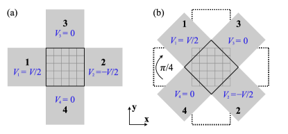
Figure 1: The schematic of a four-terminal Hall setup (a). Its four probes can be rotated by multiples of $\pi/4$, as shown in (b). The symmetry and lattice of the central scattering region (mesh grid) remain the same during the rotation.

III Numerical results and discussion

In the experiment performed on bulk T_d-MoTe₂THE2021 , the angular-resolved third-order Hall response was measured via rotating four perpendicular electrodes of a circular device. Due to the $Pmn2_{1}$ symmetry of the bulk system, the third-order Hall voltage was zero for $\theta=0,\pi/2,\pi$, etc, as shown in Fig.3c of Ref.[THE2021, ]. We propose that, one can break the mirror symmetry of MoTe₂ so that the third-order Hall response naturally exists for $\theta=0$, i.e., without rotating the electrodes. In the following, we will verify this point with both quantum nonlinear theory and the semiclassical approach.

We study the following 2D massive Dirac Hamiltonian preserving TRS:

$$H\left(\mathbf{k}\right)=A{{k}^{2}}+\left(B{{k}^{2}}+\delta\right){{\sigma}_{z}}+{{v}_{2}}{{k}_{y}}{{\sigma}_{y}}+d_{0}{{\sigma}_{x}}+\alpha k_{x}\sigma_{y},$$

where $A$, $B$, $\delta$, $v_{2}$, and $d_{0}$ are system parameters. Here $d_{0}$ determines the band gap. The presence of $v_{2}$ breaks the inversion symmetry and leaves single mirror symmetry ${\cal{M}}_{x}$ in the system. This Hamiltonian captures the key feature of monolayer T_d-MoTe₂ and T_d-WTe₂, and it is widely adopted to simulate Berry curvature related physics, including BCD and BPT. The $\alpha$ term effectively breaks the ${\cal{M}}_{x}$ symmetry. When $\alpha=0$, this system has a BCD aligning along the x-direction due to the ${\cal{M}}_{x}$ symmetry. Reference [THE2021, ] has demonstrated the BPT tensor distribution of this model in momentum space. In general, if Berry connection is zero, there is no Berry curvature related physics; if Berry curvature is zero with nonzero Berry connection, then BCD is zero and BPT is generally nonzero. Depending on the $\alpha$ term, we have two cases, $\alpha=0$ and $\alpha\neq 0$, which will be discussed in detail below. In the calculation, we conveniently set $A=0$, $B=1$, $\delta=-0.25$, $d_{0}=0.1$L-Fu1 , and $\alpha=0.1$.

Described by this Hamiltonian, the four-terminal system under investigation is shown in Fig.1. In the angle-resolved measurement, four perpendicular electrodes were rotated and the Hall current was measured as a function of the rotating angle $\theta$THE2021 . We follow the same setup in the theoretical calculation by rotating the probes while maintaining the symmetry of the central scattering region (mesh grid), as was done experimentally. Since it is difficult to deal with self-energies of the probes, only rotating angles in the increment of $\pi/4$ are considered. Numerical results on the angle-resolved Hall currents are presented in Fig.2 for the following two cases, where we fix the Fermi energy $E_{F}=0.15$ and bias voltage difference $V=0.1$.

Case 1: $\alpha=0$. In case 1, BCD exists in the system. From Fig.2(a), we observe the following: (a) The first-order Hall current is suppressed by TRS but it is nonzero due to conductivity anisotropy, and its angle-dependent properties have been theoretically explained in the supplementary of Ref. [Du2018, ] and confirmed by experimentsK-Kang ; THE2021 ; (b) The BCD-induced second-order Hall current is significant in this 2D system, since mirror symmetry ${\cal{M}}_{x}$ is preserved; (c) The third-order Hall current $I^{(3)}_{H}$ is zero for $\theta=0,\pi/2,\pi$ due to the system symmetry, and it is nonzero after $\pi/4$ rotation of the leads. $I^{(3)}_{H}$ is approximately one order of magnitude larger than the linear order Hall current $I^{(1)}_{H}$. These results qualitatively agree with the experiment for thick micron-scaled samplesTHE2021 . Notice that different orders of Hall responses are distinguishable in experiments through the phase lock-in techniqueQ-Ma ; K-Kang ; H-Yang ; THE2021 .

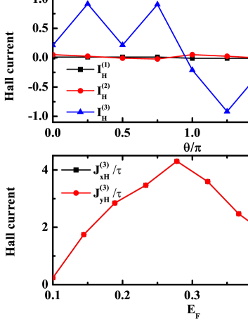
Figure 2: Angle-resolved Hall currents for the four-terminal system with $\alpha=0$ in (a) and $\alpha=0.1$ in (b). (c) shows the energy dependence of the third-order Hall current from the semiclassical approachTHE2022 without rotating the electrodes, and the current is scaled with the relaxation time $\tau$.

Case 2: $\alpha\neq 0$. In case 2, the $\alpha$ term breaks the ${\cal{M}}_{x}$ symmetry, and the system is a general noncentrosymmetric one with TRS. As one can expect, Fig.2(b) shows that the second-order Hall current almost vanishes due to the breaking of ${\cal{M}}_{x}$. BPT is less influenced, and the third-order Hall current is the dominant response in this case. Specifically, $I^{(3)}_{H}$ is nonzero at $\theta=0,\pi/2,\pi$, which means that the third-order Hall signal is observable in this 2D system without rotation of leads.

To further verify this point, we calculate the third-order Hall response $J^{(3)}_{H}$ with the semiclassical approach derived in Ref.[THE2022, ] and applied to this particular Hamiltonian [Eq.(III)]. Prediction from this semiclassical approach is presented in the Appendix. Numerical results illustrated in Fig.2(c) clearly show that the third-order Hall effect can exist in this 2D system without rotating the electrodes when the mirror symmetry is broken. It is found that the third-order Hall signals are prominent in a large energy range. As argued in Ref.[THE2022, ], in the calculation we also consider only the third-order response in linear order of the relaxation time $\tau$, since it is induced by BPT and can be more precisely extracted from experimental signals. We point out that the semiclassical approach deals with the conductivity of bulk systems, while the quantum nonlinear transport theory considers the conductances among different probes of the four-terminal setup. The quantum nonlinear transport theory also allows us to investigate the third-order Hall effect in quantum regime, which is beyond the reach of the semiclassical approach.

In the following, we study quantum characteristic of the third-order Hall current in coherent transport. In Fig.3, we plot the linear and third-order Hall currents versus the Fermi energy at the rotating angle $\theta=\pi/4$. It is found that both $I^{(1)}_{H}$ and $I^{(3)}_{H}$ changes with the Fermi energy in large ranges, and sharp current peaks are observed. As shown by the dashed lines, there is precise correspondence between the sharp peaks of $I^{(1)}_{H}$ and those of $I^{(3)}_{H}$. Remarkably, $I^{(3)}_{H}$ is significantly enhanced around the narrow peaks of $I^{(1)}_{H}$. The narrower the $I^{(1)}_{H}$ peak, the larger the $I^{(3)}_{H}$. The maximum value of $I^{(3)}_{H}$ is over 1300 in Fig.3(b), which is three to four orders of magnitude larger than $I^{(1)}_{H}$. These current peaks are similar to the resonant transmission peaks in two-probe systems, which is due to the quantum interference in coherent transport. The quantum enhancement of $I^{(3)}_{H}$ is the first quantum signature of the third-order Hall response in nanoscale systems. This common feature exists regardless of the presence or absence of mirror symmetry, suggesting that it is independent of the system symmetry.

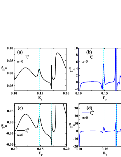
Figure 3: The linear and third-order Hall currents as a function of the Fermi energy. The rotating angle is $\pi/4$ for all panels. $\alpha=0$ in (a) and (b), and $\alpha=0.03$ in (c) and (d).

It is well known that, coherent transport can be destroyed by the dephasing effect or the phase relaxation processbut2 ; wang93 , such as thermal broadening, where sharp resonant peaks due to quantum interference are suppressed or smeared out. To further demonstrate the quantum nature of the $I^{(3)}_{H}$ peaks, we introduce dephasing mechanism into the system via the virtual probe techniquebut2 ; but3 ; datta . For simplicity, we assume that the dephasing effect only exists in the central scattering region and a virtual voltage probe is attached to each site with the zero-current constraints. The retarded self-energy of the virtual probe is $\Sigma_{i}^{r}=-i\Gamma_{i}/2$, with $\Gamma_{i}$ being the dephasing strength. After solving the nonlinear current-voltage equations for all the real and virtual probes, we obtain the third-order Hall current of the four-terminal system in the presence of dephasing, and numerical results are shown in Fig.4(a). We see that the sharp current peaks due to quantum interference are greatly reduced for the dephasing strength $\Gamma_{i}=0.01$, and coherent transport is completely suppressed for $\Gamma_{i}=0.03$. This numerical evidence proves the quantum nature of the sharp $I^{(3)}_{H}$ peaks.

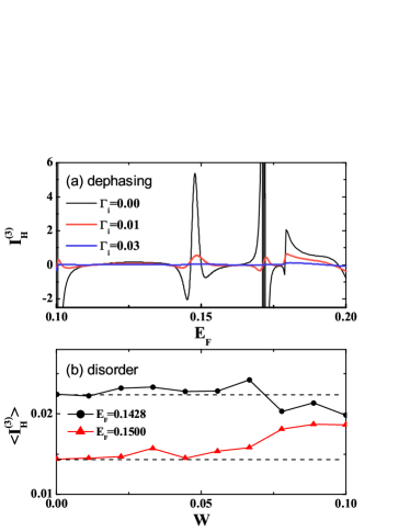
Figure 4: (a) The effect of dephasing on the third-order Hall current for several dephasing strengths. (b) Disorder-induced enhancement of the third-order Hall current for certain energies.

We also investigate the effect of disorder on the third-order Hall current. Anderson-type disorder with strength $W$ is added into the central region as random on-site energies, and the ensemble-averaged current for several Fermi energies are displayed in Fig.4(b). We find that, for certain energies, $\langle I^{(3)}_{H}\rangle$ increases with the disorder strength, which corresponds to disorder enhancement of the quantum third-order Hall current. Such enhancement is also not affected by the mirror symmetry. Similar disorder enhancement has been reported on the second-order Hall effect induced by BCD, with both semiclassicaldisorderNHE and quantum approachesQTNHE . The quantum diagrammatic theory predicted thatQTNHE , disorder effect plays decisive role in quantum second-order Hall transport. Here we numerically demonstrate that there is also disorder enhancement of the third-order Hall effect induced by BPT, which is another quantum signature of the third-order nonlinear Hall effect in quantum regime. Since both quantum interference and disorder effect are common features in quantum transport and not affected by system symmetry, it is expected that these enhancements of the third-order Hall effect widely exist in nanoscale systems.

We have studied the BCD-induced second-order Hall effect in terms of the second-order conductanceMWei , and found one-to-one corresponding nonlinear transport properties similar to the semiclassical predictionL-Fu1 . In this work, we develop the quantum third-order nonlinear transport theory, and apply it to investigate the BPT-induced third-order Hall effectTHE2021 . The numerical results qualitatively agree with experimental observations performed on bulk systems in micron scaleTHE2021 . Quantum signatures of the third-order Hall effect are revealed, which are characterized by quantum enhancement induce by quantum interference and disorder effect. The success of this quantum nonlinear transport theory in describing the second-order and third-order nonlinear Hall effects shows that it is suitable for describing nonlinear transport properties, especially in quantum regime. We emphasize that, this quantum nonlinear transport theory is a general formalism for investigating nonlinear transport through multi-terminal systems, regardless of the system symmetry.

IV Conclusion

In summary, we have developed a quantum nonlinear transport theory to study the third-order nonlinear Hall effect of a 2D four-terminal system with time-reversal symmetry. Angle-resolved Hall currents obtained from the quantum nonlinear theory on a model monolayer MoTe₂ system are qualitatively consistent with the experimental results for bulk MoTe₂. More importantly, it is found that in coherent transport, the third-order Hall current can be significantly enhanced by quantum interference to three orders of magnitude larger than the first-order Hall signal. Such quantum enhancement is vulnerable to dephasing effect. We also find disorder-induced enhancement of the third-order Hall current in quantum transport. These numerical findings highlight quantum characteristics of the third-order Hall effect induced by BPT, and we expect that experimental observations can be carried out on platforms such as nanoscale MoTe₂ and TaIrTe₄.

V Appendix: The semiclassical approach for the third-order current

According to the extended semiclassical approach in Ref.[THE2022, ], the third-order current is expressed as ($\hbar=e=1$)

$$\begin{split}{{J}^{\left(3\right)}}=&-\tau\int{\left[d\textbf{k}\right]}{{\nabla}_{\textbf{k}}}\varepsilon\left(\textbf{E}\cdot{{\nabla}_{\textbf{k}}}\right)\left[{{\varepsilon}^{\left(2\right)}}f_{0}^{{}^{\prime}}\right]\\ &-\tau\int{\left[d\textbf{k}\right]}{{\nabla}_{\textbf{k}}}{{\varepsilon}^{\left(2\right)}}\left(\textbf{E}\cdot{{\nabla}_{\textbf{k}}}\right){{f}_{0}}\\ &-\tau\int{\left[d\textbf{k}\right]}\textbf{E}\times{{\mathbf{\Omega}}^{\left(1\right)}}\left(\textbf{E}\cdot{{\nabla}_{\textbf{k}}}\right){{f}_{0}}\\ &-{\tau^{3}}\int{\left[{d\textbf{k}}\right]}{\nabla_{\textbf{k}}}\varepsilon{\left({\textbf{E}\cdot{\nabla_{\textbf{k}}}}\right)^{3}}{f_{0}},\end{split}$$

where ${{\varepsilon}^{\left(2\right)}}=-\frac{1}{2}\textbf{E}\overset{\lower 5.0pt\hbox{$\smash{\scriptscriptstyle\leftrightarrow}$}}{G}\textbf{E}$ is the second-order correction to energy, ${{G}_{ab}}=2\operatorname{Re}\sum\limits_{n\neq 0}{\frac{{{\left({{A}_{a}}\right)}_{0n}}{{\left({{A}_{b}}\right)}_{n0}}}{{{\varepsilon}_{0}}-{{\varepsilon}_{n}}}}$ is the Berry-connection polarizability tensor (BPT) with the interband Berry connection ${{\left({{A}_{a}}\right)}_{mn}}=\left\langle{{u}_{m}}\left|i{{\partial}_{k_{a}}}\left|{{u}_{n}}\right.\right.\right\rangle$, and ${{\Omega}^{\left(1\right)}}={{\nabla}_{\textbf{k}}}\times\overset{\lower 5.0pt\hbox{$\smash{\scriptscriptstyle\leftrightarrow}$}}{G}\textbf{E}$ is the field-induced Berry curvature.

Considering only the linear term in $\tau$ since the third-order term in $\tau$ is a Drude-like contribution, the third-order current is simplified as

$$\begin{split}{{J}^{\left(3\right)}}=&-\tau[\int{\left[d\mathbf{k}\right]}\frac{\hbar}{2}{{v}_{0}}\left(\mathbf{E}G\mathbf{E}\right)\left(\mathbf{E}\cdot{{\partial}_{\mathbf{k}}}\right){{f}_{0}}^{\prime}\\ &+\int{\left[d\mathbf{k}\right]}{{\nabla}_{\mathbf{k}}}\times{{\mathbf{\Omega}}^{\left(1\right)}}\left(\mathbf{E}\cdot{{\partial}_{\mathbf{k}}}\right){{f}_{0}}].\\ \end{split}$$ (25)

For the 2D Dirac model defined in Eq.(III), the current along $y$ direction is

$$\begin{split}J_{y}^{\left(3\right)}=&-\tau[\int{\left[d\mathbf{k}\right]}\frac{\hbar}{2}{{v}_{0}}\left(\mathbf{E}G\mathbf{E}\right)\left(\mathbf{E}\cdot{{\partial}_{\mathbf{k}}}\right){{f}_{0}}^{\prime}\\ &+\int{\left[d\mathbf{k}\right]}{{\left({{\nabla}_{\mathbf{k}}}\times{{\mathbf{\Omega}}^{\left(1\right)}}\right)}_{y}}\left(\mathbf{E}\cdot{{\partial}_{\mathbf{k}}}\right){{f}_{0}}]\\ =&-\tau[\int{\left[d\mathbf{k}\right]}{{\chi}_{yxxx}}E_{x}^{3}+{{\chi}_{yxxy}}E_{x}^{2}{{E}_{y}}\\ &+{{\chi}_{yxyy}}{{E}_{x}}E_{y}^{2}+{{\chi}_{yyyy}}E_{y}^{3}]\\ \end{split}$$ (26)

where

$$\begin{split}{\chi_{yxxx}}=&\left({{\partial_{y}}{G_{xx}}-{\partial_{x}}{G_{xy}}}\right){\partial_{x}}{f_{0}}+\frac{\hbar}{2}{v_{0}}{G_{xx}}{\partial_{x}}{f_{0}}^{\prime},\\ {\chi_{yxxy}}=&\left({{\partial_{y}}{G_{xy}}-{\partial_{x}}{G_{yy}}}\right){\partial_{x}}{f_{0}}+\left({{\partial_{y}}{G_{xx}}-{\partial_{x}}{G_{xy}}}\right){\partial_{y}}{f_{0}}\\ +&\frac{\hbar}{2}{v_{0}}\left({2{G_{xy}}{\partial_{x}}{f_{0}}^{\prime}+{G_{xx}}{\partial_{y}}{f_{0}}^{\prime}}\right),\\ {\chi_{yxyy}}=&\left({{\partial_{y}}{G_{xy}}-{\partial_{x}}{G_{yy}}}\right){\partial_{y}}{f_{0}}\\ +&\frac{\hbar}{2}{v_{0}}\left({{G_{yy}}{\partial_{x}}{f_{0}}^{\prime}+2{G_{xy}}{\partial_{y}}{f_{0}}^{\prime}}\right),\\ {\chi_{yyyy}}=&\frac{\hbar}{2}{v_{0}}{G_{yy}}{\partial_{y}}{f_{0}}^{\prime}.\end{split}$$

When an electric field is applied in $x$ direction, the third-order Hall current along $y$ direction is

$$J_{yH}^{\left(3\right)}=-\tau\int{\left[d\textbf{k}\right]}{{\chi}_{yxxx}}E_{x}^{3}.$$ (27)

Similarly, for an electric field along $y$ direction, the Hall current along $x$ direction is

$$J_{xH}^{\left(3\right)}=-\tau\int{\left[d\textbf{k}\right]}{{\chi}_{xyyy}}E_{y}^{3},$$ (28)

where ${{\chi}_{xyyy}}=\left({{\partial}_{x}}{{G}_{yy}}-{{\partial}_{y}}{{G}_{xy}}\right){{\partial}_{x}}{{f}_{0}}+\frac{\hbar}{2}{{v}_{0}}{{G}_{yy}}{{\partial}_{y}}{{f}_{0}}^{\prime}$. In the calculation, we set $E_{x}=E_{y}=1$ and scale the current with $\tau$. Then the third-order Hall currents are further simplified as

$$J^{(3)}_{xH}/\tau =-\int{\left[d\textbf{k}\right]}{{\chi}_{xyyy}},$$

$$J^{(3)}_{yH}/\tau =-\int{\left[d\textbf{k}\right]}{{\chi}_{yxxx}}.$$ (29)

Apparently, the third-order Hall current naturally exists in this noncentrosymmetric system.

References

- (1) I. Sodemann and L. Fu, Quantum Nonlinear Hall Effect Induced by Berry Curvature Dipole in Time-Reversal Invariant Materials, Phys. Rev. Lett. 115, 216806 (2015).
- (2) T. Low, Y. Jiang, and F. Guinea, Topological currents in black phosphorus with broken inversion symmetry, Phys. Rev. B 92, 235447 (2015).
- (3) Z. Z. Du, Hai-Zhou Lu, and X. C. Xie, Nonlinear Hall effects, Nat. Rev. Phys. 3, 744 (2021).
- (4) J. Son, K.-H. Kim, Y. H. Ahn, H.-W. Lee, and J. Lee, Strain Engineering of the Berry Curvature Dipole and Valley Magnetization in Monolayer MoS2, Phys. Rev. Lett. 123, 036806 (2019).
- (5) R. Battilomo, N. Scopigno, and C. Ortix, Berry Curvature Dipole in Strained Graphene: A Fermi Surface Warping Effect, Phys. Rev. Lett. 123, 196403 (2019).
- (6) O. Matsyshyn and I. Sodemann, Nonlinear Hall Acceleration and the Quantum Rectification Sum Rule, Phys. Rev. Lett. 123, 246602 (2019).
- (7) D.-F. Shao, S.-H. Zhang, G. Gurung, W. Yang, and E. Y. Tsymbal, Nonlinear Anomalous Hall Effect for Neél Vector Detection, Phys. Rev. Lett. 124, 067203 (2020).
- (8) S.-Y. Xu, Q. Ma, H. Shen, V. Fatemi, S. Wu, T.-R. Chang, G. Chang, A. M. M. Valdivia, C.-K. Chan, Q. D. Gibson, J. Zhou, Z. Liu, K. Watanabe, T. Taniguchi, H. Lin, R. J. Cava, L. Fu, N. Gedik, and P. Jarillo-Herrero, Electrically switchable Berry curvature dipole in the monolayer topological insulator WTe2, Nat. Phys. 14, 900 (2018).
- (9) Q. Ma, S.-Y. Xu, H. Shen, D. MacNeill, V. Fatemi, T.-R. Chang, A. M. Mier Valdivia, S. Wu, Z. Du, C.-H. Hsu, S. Fang, Q. D. Gibson, K. Watanabe, T. Taniguchi, R. J. Cava, E. Kaxiras, H.-Z. Lu, H. Lin, L. Fu, N. Gedik, and P. Jarillo-Herrero, Observation of the nonlinear Hall effect under time-reversal-symmetric conditions, Nature 565, 337 (2019).
- (10) K. Kang, T. Li, E. Sohn, J. Shan, and K. F. Mak, Nonlinear anomalous Hall effect in few-layer WTe2, Nat. Mater. 18, 324 (2019).
- (11) J. Xiao, Y. Wang, H. Wang, C. D. Pemmaraju, S. Wang, P. Muscher, E. J. Sie, C. M. Nyby, T. P. Devereaux, X. Qian, X. Zhang, and A. M. Lindenberg, Berry curvature memory through electrically driven stacking transitions, Nat. Phys. 16, 1028 (2020).
- (12) D. Kumar, C.-H. Hsu, R. Sharma, T.-R. Chang, P. Yu, J. Wang, G. Eda, G. Liang, and H. Yang, Room-temperature nonlinear Hall effect and wireless radiofrequency rectification in Weyl semimetal TaIrTe4, Nat. Nanotechnol. 16, 421 (2021).
- (13) Y. Gao, S. A. Yang, and Q. Niu, Field Induced Positional Shift of Bloch Electrons and Its Dynamical Implications, Phys. Rev. Lett. 112, 166601 (2014).
- (14) Y. Gao, S. A. Yang, and Q. Niu, Geometrical effects in orbital magnetic susceptibility, Phys. Rev. B 91, 214405 (2015).
- (15) Y. Gao, S. A. Yang, and Q. Niu, Intrinsic relative magnetoconductivity of nonmagnetic metals, Phys. Rev. B 95, 165135 (2017).
- (16) H. Liu, J. Zhao, Y.-X. Huang, W. Wu, X.-L. Sheng, C. Xiao, and S. A. Yang, Intrinsic Second-Order Anomalous Hall Effect and Its Application in Compensated Antiferromagnets, Phys. Rev. Lett. 127, 277202 (2021).
- (17) S. Lai, H. Liu, Z. Zhang, J. Zhao, X. Feng, N. Wang, C. Tang, Y. Liu, K. S. Novoselov, S. A. Yang, and W.-b. Gao, Third-order nonlinear Hall effect induced by the Berry-connection polarizability tensor, Nat. Nanotechnol. 16, 869 (2021).
- (18) C. Wang, R.-C. Xiao, H. Liu, Z. Zhang, S. Lai, C. Zhu, H. Cai, N. Wang, S. Chen, Y. Deng, Z. Liu, S. A. Yang, W.-b. Gao, Room temperature third-order nonlinear Hall effect in Weyl semimetal TaIrTe4, Natl. Sci. Rev, nwac020 (2022), doi: 10.1093/nsr/nwac020.
- (19) S. Roy and A. Narayan, Non-linear Hall effect in multi-Weyl semimetals, J. Phys.: Condens. Matter, to be published, doi: 10.1088/1361-648X/ac8091.
- (20) H. Liu, J. Zhao, Y.-X. Huang, X. Feng, C. Xiao, W. Wu, S. Lai, W.-b. Gao, and S. A. Yang, Berry connection polarizability tensor and third-order Hall effect, Phys. Rev. B 105, 045118 (2022).
- (21) C.-P. Zhang, X.-J. Gao, Y.-M. Xie, H. C. Po, and K. T. Law, Higher-order nonlinear anomalous Hall effects induced by Berry curvature, arXiv:2012.15628.
- (22) Z. Z. Du, C. M. Wang, S. Li, H. -Z. Lu, and X.C. Xie, Disorder-induced nonlinear Hall effect with time-reversal symmetry, Nat. Commun. 10, 3047 (2019).
- (23) Z. Z. Du, C. M. Wang, H. -P. Sun, H. -Z. Lu, and X.C. Xie, Quantum theory of the nonlinear Hall effect, Nat. Commun. 12, 5038 (2021).
- (24) M. Büttiker, Capacitance, admittance, and rectification properties of small conductors, J. Phys.: Condens. Matter 5, 9361 (1993).
- (25) M. Büttiker and T. Christen, Basic elements of electrical conduction, in Quantum Transport in Semiconductor Submicron Structures, edited by B. Kramer, (Kluwer Academic Publishers, Dordrecht, 1996, pp.263-291).
- (26) T. Gramespacher and M. Büttiker, Nanoscopic tunneling contacts on mesoscopic multiprobe conductors, Phys. Rev. B 56, 13026 (1997).
- (27) Z. S. Ma, J. Wang and H. Guo, Weakly nonlinear ac response: Theory and application, Phys. Rev. B 59, 7575 (1999).
- (28) B. Wang, J. Wang and H. Guo, Nonlinear I-V characteristics of a mesoscopic conductor, J. Appl. Phys. 86, 5094 (1999).
- (29) V. Gasparian, T. Christen, and M. Büttiker, Partial densities of states, scattering matrices, and Green’s functions, Phys. Rev. A 54, 4022 (1996).
- (30) Y. Wei and J. Wang, Current conserving nonequilibrium ac transport theory, Phys. Rev. B 79, 195315 (2009).
- (31) is defined below Eq.(1).
- (32) Z. Z. Du, C. M. Wang, H.-Z. Lu, and X. C. Xie, Band signatures for strong nonlinear Hall effect in bilayer WTe2, Phys. Rev. Lett. 121, 266601 (2018).
- (33) M. Büttiker, Role of quantum coherence in series resistors, Phys. Rev. B 33, 3020 (1986).
- (34) Y. J. Wang, J. Wang, and H. Guo, Effects of inelastic processes on the transmission in a coupled-quantum-wire system, Phys. Rev. B 47, 4348 (1993).
- (35) M. Moskalets and M. Büttiker, Effect of inelastic scattering on parametric pumping, Phys. Rev. B 64, 201305(R) (2001).
- (36) R. Golizadeh-Mojarad and S. Datta, Nonequilibrium Green’s function based models for dephasing in quantum transport, Phys. Rev. B 75, 081301(R) (2007).
- (37) M. Wei, B. Wang, Y. Yu, F. Xu, and J. Wang, Nonlinear Hall effect induced by internal Coulomb interaction and phase relaxation process in a four-terminal system with time-reversal symmetry, Phys. Rev. B 105, 115411 (2022).