Simultaneous Inference for Time Series Functional Linear Regression

Abstract

We consider the problem of joint simultaneous confidence band (JSCB) construction for regression coefficient functions of time series scalar-on-function linear regression when the regression model is estimated by roughness penalization approach with flexible choices of orthonormal basis functions. A simple and unified multiplier bootstrap methodology is proposed for the JSCB construction which is shown to achieve the correct coverage probability asymptotically. Furthermore, the JSCB is asymptotically robust to inconsistently estimated standard deviations of the model. The proposed methodology is applied to a time series data set of electricity market to visually investigate and formally test the overall regression relationship as well as perform model validation.

Keywords: Convex Gaussian approximation; Functional time series; Joint simultaneous confidence band; Multiplier bootstrap; Roughness penalization.

1 Introduction

It is increasingly common to encounter time series that are densely observed over multiple oscillation periods or natural consecutive time intervals. To address statistical issues with respect to data structures such as the aforementioned, functional (or curve) time series analysis has undergone unprecedented development over the last two decades. See [27] and [6] for excellent book-length treatments of the topic. We also refer the readers to [26], [3, 2], [43], [42] and [16] among many others for articles that address various modelling, estimation, forecasting and inference aspects of functional time series analysis from both time and spectral domain perspectives.

The main purpose of this article is to perform simultaneous statistical inference for time series scalar-on-function linear regression. Specifically, consider the following time series functional linear model (FLM):

$$Y_{i}=\beta_{0}+\sum_{j=1}^{p}\int_{0}^{1}\beta_{j}(t)X_{ij}(t)\mathrm{d}t+\epsilon_{i},~{}~{}i=1,...,n,$$ (1)

where $\{\bm{X}_{i}(t):=(X_{i1}(t),...,X_{ip}(t))^{\top}\}_{i=1}^{n}$ is a $p$-variate stationary time series of known functional predictors observed on $[0,1]$, $\{Y_{i}\}_{i=1}^{n}$ is a univariate stationary time series of responses, and $\{\epsilon_{i}\}_{i=1}^{n}$ is a centered stationary time series of regression errors satisfying $\mathbb{E}[X_{ij}(t)\epsilon_{i}]=0$ for all $t\in[0,1]$ and $j=1,2,...,p$. Observe that $\bm{X}_{i}(t)$ and $\epsilon_{i}$ could be dependent and $\beta_{0}+\sum_{j=1}^{p}\int_{0}^{1}\beta_{j}(t)X_{ij}(t)\mathrm{d}t$ can be viewed as the best linear forecast of $Y_{i}$ based on $\bm{X}_{i}(t)$. We are interested in constructing asymptotically correct joint simultaneous confidence bands (JSCB) for the regression coefficients $\bm{\beta}(t):=(\beta_{1}(t),...,\beta_{p}(t))^{\top}$; that is, we aim to find random functions $L_{n,j}(t)$ and $U_{n,j}(t)$, $j=1,2,...,p$, such that

$$\lim_{n\rightarrow\infty}\mathbb{P}\Big{(}L_{n,j}(t)\leq\beta_{j}(t)\leq U_{n,j}(t),~{}\mbox{for all }t\in[0,1]~{}\mbox{and }j=1,2,...,p\Big{)}=1-\alpha$$

for a pre-specified coverage probability $1-\alpha$. The need for JSCB arises in many situations when one wants to, for instance, rigorously investigate the overall magnitude and pattern of the regression coefficient functions, test various assumptions on the regression relationship and perform diagnostic checking and model validation of (1) without multiple hypothesis testing problems.

To date, results for the time series scalar-on-function regression (1) are scarce and are mainly on the consistency of functional principle component (FPC) based estimators ([26], [25]). To our knowledge, there is no literature on asymptotically correct JSCB construction for $\bm{\beta}(t)$ under time series dependence. On the other hand, there is a wealth of statistics literature dealing with estimation, convergence rate investigation, prediction, and application of FLM (1) when the data $\{(Y_{i},\bm{X}_{i}(t))\}_{i=1}^{n}$ are independent and identically distributed (i.i.d.). See, for instance, [8], [15], [34], [7] and [31] for a far from exhaustive list of references. We also refer the readers to [9], [40], [56] and [46] for excellent recent reviews of the topic and more references. Meanwhile, the last two decades also witnessed an increase in statistics literature on the inference of FLM (1) for independent data. Since a JSCB is primarily an inferential tool, we shall review this literature in more detail. The main body of the aforementioned literature consists of results related to ${\cal L}^{2}$-type tests on whether $\bm{\beta}(t)=0$ or a fixed known function; see for instance [24], [33], [32] and [52], among others. Other contributions include confidence interval construction for the conditional mean and hypothesis testing for functional contrasts ([50]) and goodness of fit tests for (1) versus possibly nonlinear alternatives ([28], [21], [38]). On the other hand, however, to our knowledge for independent observations there are few results discussing confidence band construction for $\bm{\beta}(t)$. [30] proposed a simple methodology to construct a conservative confidence band for the slope function of scalar-on-function linear regression for independent data which covers “most” of points; Recently, [17] constructed an asymptotically correct simultaneous confidence band for function-on-function linear regression of independent data and the authors also discussed the scalar-on-function case briefly. The implementation of the latter paper requires estimating the convergence rate of the regression which could be a relatively difficult task in moderate samples.

There are two major challenges involved with JSCB construction of $\bm{\beta}(t)$ for the time series FLM (1). Firstly, estimation of model (1) is related to an ill-posed inverse problem ([9], Section 2.2) and often estimators of $\bm{\beta}(t)$ are not tight on $[0,1]$. As a result, it has been a difficult problem to investigate the large sample distributional behavior of estimators of $\bm{\beta}(t)$ uniformly across $t$. Secondly, the rates of convergence for various estimators of $\bm{\beta}(t)$ depend sensitively on the smoothness of $\bm{X}_{i}(t)$ and $\bm{\beta}(t)$, and the penalization parameter used in the regression. Consequently, in practice it is difficult to determine the latter rates of convergence and hence the appropriate normalizing constants for the uniform inference of $\bm{\beta}(t)$. In this article, we address the aforementioned challenges by proposing a simple and unified multiplier bootstrap methodology for the JSCB construction. For the roughness penalized estimators of $\bm{\beta}(t)$, the multiplier bootstrap will be shown to well approximate their weighted maximum deviations on $[0,1]$ uniformly across all quantiles and a wide class of smooth weight functions under quite general conditions in large samples. As a result, the bootstrap allows to construct asymptotically correct JSCB for $\bm{\beta}(t)$ in a simple and unified way without having to derive the uniform distributional behavior or rates of convergence. Furthermore, the JSCB constructed by the multiplier bootstrap remains asymptotically correct when the weight function is estimated inconsistently under some mild conditions, adding another layer of robustness to the methodology. Theoretically, validation of the bootstrap depends critically on uniform Gaussian approximation and comparison results over all Euclidean convex sets for sums of stationary and weakly dependent time series of moderately high dimensions which we will establish in this paper. These results extend the corresponding findings for independent or $m$-dependent data investigated in [5], [20] and [19] among others.

The multiplier/weighted bootstrap technique has attracted much attention recently. Among others, [10] derived asymptotic consistency of the generalized bootstrap technique for estimating equations. [37] established the validity of the weighted bootstrap technique based on a weighted $M$-estimation framework. Non-asymptotic results on the multiplier bootstrap validity with applications to high-dimensional inference of independent data were established in [12]. Later, [51] considered a multiplier bootstrap procedure in the construction of likelihood-based confidence sets under possible model misspecifications.

The paper is organized as follows. In Section 2, we propose the methodology of the JSCB construction based on roughness penalization approach. The theoretical result on the multiplier bootstrap for estimators of $\bm{\beta}(t)$ by roughness penalization estimation is discussed in Section 3. In particular, we introduce in Section 3.1 a general class of stationary functional time series models based on orthonormal basis expansions and nonlinear system theory. Section 4 investigates finite sample accuracy of the bootstrap methodology for various basis functions and weighting schemes using Monte Carlo experiments. We analyze a time series dataset on electricity demand curves and daily total demand in Spain in Section 5 and conclude the article in Section 6 with discussions on several issues including the effects of pre-smoothing, practical choices of the basis functions and extensions to regression models with functional response. Additional simulations, examples, theoretical results and the proofs of all theoretical results are deferred to the supplemental material.

2 Methodology

Hereafter, for simplicity we shall assume that $Y_{i}$ and $\bm{X}_{i}(t)$ are centered and hence $\beta_{0}=0$. Let $H=\mathcal{L}^{2}([0,1])$ be the Hilbert space of all square integrable functions on $[0,1]$ with inner product $\langle x,y\rangle=\int_{0}^{1}x(t)y(t)\mathrm{d}t$. We also denote by $\mathcal{C}^{d}([0,1])$ the collection of functions that are $d$-times continuously differentiable with absolutely continuous $d$-th derivative on $[0,1]$.

2.1 Roughness Penalization Estimation

In order to facilitate the formulation of roughness penalization estimation, we first prepare some notations. Throughout this paper, we assume that $X_{ij}(t)$ for $j=1,...,p,~{}i=1,...,n$ is continuous on $[0,1]$ a.s. and hence admits the following expansion $X_{ij}(t)=\sum_{k=1}^{\infty}\widetilde{x}_{ij,k}\alpha_{k}(t),$ where $\{\alpha_{k}(t)\}_{k=1}^{\infty}$ is a set of pre-selected orthonormal basis functions of $H$. From Theorem 1 of [49], $X_{ij}(t)$ has the standard Karhunen-Loève type expansion as follows

$$X_{ij}(t)=\sum_{k=1}^{\infty}f_{jk}x_{ij,k}\alpha_{k}(t),$$ (2)

where $f_{jk}={\rm Std}(\widetilde{x}_{ij,k})$ with ${\rm Std}$ denoting standard deviation and $x_{ij,k}=\widetilde{x}_{ij,k}/f_{jk}$ if $f_{jk}\neq 0$. Set $x_{ij,k}=0$ if $f_{jk}=0$. Notice that $f_{jk}$ captures the decay speed of $\widetilde{x}_{ij,k}$ as $k$ increases and the random coefficient $\{x_{ij,k}\}_{k=1}^{\infty}$ remains at the same magnitude with variance $1$ as $k$ increases if $f_{jk}\neq 0$. Similarly, write $\beta_{j}(t)=\sum_{k=1}^{\infty}\beta_{jk}\alpha_{k}(t).$ The following assumption restricts the decay speed of the basis expansion coefficients of $\{\bm{X}_{i}(t)\}$ and $\{\bm{\beta}(t)\}$.

Assumption 2.1.

For some non-negative integers $d_{1}$ and $d_{2}$ with $d_{1}\geq d_{2}$, assume that $\beta_{j}(t)\in\mathcal{C}^{d_{1}}([0,1])$ and $X_{ij}(t)\in\mathcal{C}^{d_{2}}([0,1])$ a.s.. Suppose that $|\beta_{jk}|\leq C_{1}k^{-(d_{1}+1)}$, $\forall j=1,...,p$ and $C_{1}>0$ is some finite constant, the random coefficient $\widetilde{x}_{ij,k}=\mathcal{O}_{a.s.}(k^{-(d_{2}+1)})$ for $i=1,...,n,~{}j=1,...,p$.

Let $d\geq 0$ be an integer. It is well-known that for a general $\mathcal{C}^{d}([0,1])$ function the fastest decay rate for its $k$-th basis expansion coefficient is $O(k^{-d-1})$ for a wide class of basis functions ([11]). For instance, the Fourier basis (for periodic functions), the weighted Chebyshev polynomials ([53]) and the orthogonal wavelets with degree $m\geq d$ ([39]) admit the latter decay rate under some extra mild assumptions on the behavior of the function’s $d$-th derivative. Hence Assumption 2.1 essentially requires that the basis expansion coefficients of $\beta_{j}(t)$ and $X_{ij}(t)$ decay at the fastest rate. On the other hand, we remark that the basis expansion coefficients may decay at slower speeds for some orthonormal bases. An example is the Legendre polynomials where the coefficients decay at an $O(k^{-d-1/2})$ speed ([55]). For basis functions whose coefficients decay at slower rates, following the proofs of this paper it is obvious to see that the multiplier bootstrap method for the JSCB construction is still asymptotically valid under the corresponding restrictions on the tuning parameters. However, in this case the estimates of $\bm{\beta}(t)$ will converge at a slower speed and the bootstrap approximation may be less accurate. For the sake of brevity we shall stick to the fastest decay Assumption 2.1 for our theoretical investigations throughout this paper.

The roughness penalization approach to the FLM (1) solves the following penalized least squares problem

$$\widetilde{\bm{\beta}}(t)=\mathop{\arg\min}_{\bm{\beta}(t)}\left\{\frac{1}{n}\sum_{i=1}^{n}\left[Y_{i}-\sum_{j=1}^{p}\int_{0}^{1}\beta_{j}(t)X_{ij}(t)\mathrm{d}t\right]^{2}+\lambda\sum_{j=1}^{p}\int_{0}^{1}[\beta^{\prime\prime}_{j}(t)]^{2}\mathrm{d}t\right\},$$ (3)

see [50] and references therein. On the other hand, in functional data analysis, researchers usually work on the optimization problem on a finite-dimensional subspace ([34]), which makes the procedure easily implementable. Following the method proposed by [45], we truncate the coefficient functions to finite (but diverging) dimensional spans of a priori set of basis functions $\{\alpha_{k}(t)\}_{k=1}^{\infty}$ while involving a smoothness penalty. Specifically, assume the truncation number of $\beta_{j}(t)$ equals $c_{j}$ ($c_{j}\rightarrow\infty$). Then the right hand side of (3) can be approximated by

$$\frac{1}{n}\sum_{i=1}^{n}\left[Y_{i}-\sum_{j=1}^{p}\int_{0}^{1}\beta_{j,c_{j}}(t)X_{ij}(t)\mathrm{d}t\right]^{2}+\lambda\sum_{j=1}^{p}\int_{0}^{1}[\beta^{\prime\prime}_{j,c_{j}}(t)]^{2}\mathrm{d}t,$$

where $\beta_{j,c_{j}}(t)=\sum_{k=1}^{c_{j}}\beta_{jk}\alpha_{k}(t)$. Simplifying the above expression, the estimation can be achieved by minimizing the following penalized least squares criterion function

$$\frac{1}{n}\sum_{i=1}^{n}\left[Y_{i}-\sum_{j=1}^{p}\sum_{k=1}^{c_{j}}\beta_{jk}\widetilde{x}_{ij,k}\right]^{2}+\lambda\sum_{j=1}^{p}\sum_{k,l=1}^{c_{j}}\beta_{jk}\beta_{jl}\widetilde{R}_{j}(k,l)$$

$$= \frac{1}{n}[\bm{Y}-\bm{X}_{c}\bm{\theta}_{c}]^{\top}[\bm{Y}-\bm{X}_{c}\bm{\theta}_{c}]+\bm{\theta}_{c}^{\top}\bm{R}(\lambda)\bm{\theta}_{c},$$ (4)

where $\lambda$ ($\lambda\rightarrow 0$) is a common smoothing parameter that measures the rate of exchange between fit to the data and smoothness of the estimator, as measured by the residual sum of squares in the first term, and variability of the functions $\beta_{j,c_{j}}(t)$ in the second term. Here we impose a roughness penalty associated with the same smoothing parameter $\lambda$ for every $j$, which is commonly used in practice, see [18].

In (4), $c=c(n)=\sum_{j=1}^{p}c_{j}$ and $\bm{\theta}_{c}$ is a $c$-dimensional block vector where $\bm{\theta}_{j}^{c}=(\theta_{j1},...,\theta_{jc_{j}})^{\top}$ is the $j$-th block with $\theta_{jk}=f_{jk}\beta_{jk}$ for $k=1,...,c_{j}$. Furthermore, $\bm{X}_{c}$ is the $n\times c$ block design matrix, $\bm{R}(\lambda)$ is a $c\times c$ block diagonal matrix with $\lambda\bm{R}_{j}$ as its diagonals and $\bm{R}_{j}$ is a $c_{j}\times c_{j}$ matrix with elements $R_{j}(k,l)=\int_{0}^{1}\alpha_{k}^{\prime\prime}(t)\alpha_{l}^{\prime\prime}(t)\mathrm{d}t/(f_{jk}f_{jl})$. Then the penalized least squares estimator turns out to be

$$\widetilde{\bm{\theta}}_{c}=\left[\frac{\bm{X}_{c}^{\top}\bm{X}_{c}}{n}+\bm{R}(\lambda)\right]^{-1}\frac{\bm{X}_{c}^{\top}\bm{Y}}{n}.$$

Consequently, it is easy to find the matrix representation of the roughness penalized estimator $\widetilde{\bm{\beta}}(t)=\bm{C}_{f}(t)\widetilde{\bm{\theta}}_{c},$ where $\bm{C}_{f}(t)=(\bm{C}_{1}^{\top}(t),...,\bm{C}_{p}^{\top}(t))$ is a $p\times c$ matrix and $\bm{C}_{j}(t)$ is a $c$-dimensional block vector with $(\alpha_{1}(t)/f_{j1},...,\alpha_{c_{j}}(t)/f_{jc_{j}})^{\top}$ as its $j$-th block and other elements being 0.

2.2 JSCB Construction

JSCB construction of $\bm{\beta}(t)$ boils down to evaluating the distributional behavior of the weighted maximum deviation

$$\Xi_{n,\bm{g}_{n}}:=\sqrt{n}\sup_{t\in[0,1]}|\widetilde{\bm{\beta}}(t)-\bm{\beta}(t)|_{\bm{g}_{n}(t)},$$

where $|\bm{V}(t)|_{\bm{g}(t)}=\max_{1\leq j\leq p}|V_{j}(t)/g_{j}(t)|$ for any function $\bm{V}(t)=(V_{1}(t),\\ ...,V_{p}(t))^{\top}$ and weight function $\bm{g}(t)=(g_{1}(t),...,g_{p}(t))^{\top}$. The weight function $\bm{g}_{n}(t)$ is assumed to belong to a class $\mathcal{G}$ with

$$\mathcal{G} =\{\bm{f}(t):[0,1]\to\mathbb{R}^{p},~{}\bm{f}=(f_{1},...,f_{p})^{\top}~{}\text{is a continuous}~{}p\text{-dimensional}$$

$$\text{~{}vector~{}function~{}satisfying}\inf_{t\in[0,1]}\min_{1\leq j\leq p}f_{j}(t)\geq\kappa\text{~{}for some constant}~{}\kappa>0\}.$$

For a given $\alpha\in(0,1)$, denote by $\xi_{n,\bm{g}_{n}}(\alpha)$ the $(1-\alpha)$-th quantile of $\Xi_{n,\bm{g}_{n}}$. Then a JSCB with coverage probability $1-\alpha$ can be constructed as $\widetilde{\beta}_{j}(t)\pm\xi_{n,\bm{g}_{n}}(\alpha)g_{nj}(t)/\sqrt{n}$, $t\in[0,1]$, $j=1,2,...,p$.

Observe that the width of the JSCB is proportional to the weight function $\bm{g}_{n}(t)$. In practice one could simply choose some fixed weight functions such as $g_{nj}(t)\equiv 1$ which yields equal JSCB width at each $t$ and $j$. Alternatively, when the sample size is sufficiently large and temporal dependence is weak or moderately strong, we recommend choosing $g_{nj}(t)={\rm Std}(\widetilde{\beta}_{j}(t))/\int_{0}^{1}{\rm Std}(\widetilde{\beta}_{j}(s))\mathrm{d}s,~{}j=1,...,p.$ There are two advantages for this data-driven choice of weights. First, the resulting width of the JSCB reflects the standard deviation of $\widetilde{\bm{\beta}}(t)$ which gives direct visual information on the estimation uncertainty at every $t\in[0,1]$ and $j=1,...,p$. Second, this choice of weight function yields much smaller average width of the JSCB compared to some fixed choices such as $\bm{g}_{n}(t)\equiv 1$; see our simulations in Section 4 for a finite-sample illustration. On the other hand, ${\rm Std}(\widetilde{\beta}_{j}(t))$ has to be estimated in practice. Later in this article, we shall discuss its estimation and also asymptotic robustness of our multiplier bootstrap methodology when the weight function is inconsistently estimated.

To motivate the multiplier bootstrap, denote $\widetilde{\bm{\Sigma}}_{c}(\lambda)=\bm{X}_{c}^{\top}\bm{X}_{c}/n+\bm{R}(\lambda)$. Note that $\widetilde{\bm{\Sigma}}_{c}(\lambda)\approx\frac{\mathbb{E}(\bm{X}_{c}^{\top}\bm{X}_{c})}{n}+\bm{R}(\lambda):=\bm{\Sigma}_{c}(\lambda)$ under mild conditions. For simplicity, we assume that each $\beta_{j}(t)$ has the same degree of smoothness, here we let each $c_{j}$ have the same rate of divergence. By elementary calculations and basis expansions, we have

$$\widetilde{\bm{\beta}}(t)-\bm{\beta}(t)=\bm{C}_{f}(t)\widetilde{\bm{\Sigma}}_{c}^{-1}(\lambda)\frac{\bm{X}_{c}^{\top}\widetilde{\bm{\epsilon}}}{n}-\bm{C}_{f}(t)\widetilde{\bm{\Sigma}}_{c}^{-1}(\lambda)\bm{R}(\lambda)\bm{\theta}_{c}+\mathcal{O}(c^{-d_{1}}),$$ (5)

where $\widetilde{\bm{\epsilon}}=(\epsilon_{1}+\mathcal{O}_{\mathbb{P}}(c^{-(d_{1}+d_{2}+1)}),...,\epsilon_{n}+\mathcal{O}_{\mathbb{P}}(c^{-(d_{1}+d_{2}+1)}))^{\top}$. Hence if $c$ is sufficiently large and $\lambda$ is relatively small such that $\widetilde{\bm{\beta}}(t)$ is under-smoothed, i.e., the standard deviation of the estimation (captured by the first term on the right hand side of (5)) dominates the bias asymptotically, Eq.(5) reveals that the maximum deviation of $\sqrt{n}\widetilde{\bm{\beta}}(t)$ on $[0,1]$ is determined by the uniform probabilistic behavior of $\bm{Q}_{n}^{z}(t,\lambda):=\bm{C}_{f}(t)\bm{\Sigma}_{c}^{-1}(\lambda)\bm{Z}_{n}^{c}$, where $\bm{Z}_{n}^{c}:=\frac{1}{\sqrt{n}}\sum_{i=1}^{n}\bm{z}_{ci}$ and $\bm{z}_{ci}=\bm{x}_{ci}\epsilon_{i}$ with $\bm{x}_{ci}$ being the $i$-th column of $\bm{X}_{c}^{\top}$.

There are two major difficulties in the investigation of $\bm{Q}_{n}^{z}(t,\lambda)$ uniformly in $t$. Firstly, $\{\bm{z}_{ci}\}_{i\in\mathbb{Z}}$ is typically a moderately high-dimensional time series whose dimensionality $c$ diverges slowly with $n$ and $\bm{Q}_{n}^{z}(t,\lambda)$ is not a tight sequence of stochastic processes on $[0,1]$. Consequently, deriving the explicit limiting distribution of the maximum deviation of $\bm{Q}_{n}^{z}(t,\lambda)$ is a difficult task. Second, the convergence rate of $\sup_{t\in[0,1]}|\bm{Q}_{n}^{z}(t,\lambda)|_{\bm{g}_{n}(t)}$ depends on many nuisance parameters such as the smoothness of $\bm{X}_{i}(t)$ and $\bm{\beta}(t)$, and the diverging rate of the truncation parameters $c_{j}$, which are difficult to estimate in practice. To circumvent the aforementioned difficulties, one possibility is to utilize certain bootstrap methods to avoid deriving and estimating the limiting distributions and nuisance parameters explicitly. In this article, we resort to the multiplier/wild/weighted bootstrap ([57]) to mimic the probabilistic behavior of the process $\bm{Q}_{n}^{z}(t,\lambda)$ uniformly over $t$. In the literature, the multiplier bootstrap has been used for high dimensional inference on hyper-rectangles and certain classes of simple convex sets that can be well approximated by (possibly higher dimensional) hyper-rectangles after linear transformations; see for instance [12] and [14] for independent data and [64] for functional time series. The inference of $\sup_{t\in[0,1]}|\bm{Q}_{n}^{z}(t,\lambda)|_{\bm{g}_{n}(t)}$ uniformly over all quantiles and weight functions in $\mathcal{G}$ can be transformed into investigating the probabilistic behavior of $\bm{Z}_{n}^{c}$ over a large class of moderately high-dimensional convex sets. However, these convex sets have complex geometric structures for which results that are based on approximations on hyper-rectangles and their linear transformations are not directly applicable. As a result, in this article we shall extend the uniform Gaussian approximation and comparison results over all high-dimensional convex sets for sums of independent and $m$-dependent data established in, for instance, [5], [20] and [19] to sums of stationary and short memory time series in order to validate the multiplier bootstrap. These results may be of wider applicability in other moderately high-dimensional time series problems.

To be more specific, we will consider the bootstrapped sum given a block size $m$: $\bm{U}_{n}^{boots}=\frac{1}{\sqrt{n-m+1}}\sum_{j=1}^{n-m+1}\left(\frac{1}{\sqrt{m}}\sum_{i=j}^{j+m-1}\bm{z}_{ci}\right)u_{j},$ where $\{u_{j}\}_{j=1}^{n-m+1}$ is a sequence of i.i.d. standard normal random variables which is independent of $\bm{Z}_{1}^{n}:=\{\bm{z}_{c1},...,\bm{z}_{cn}\}$. Define $\bm{Q}_{n}^{boots}(t,\lambda)=\bm{C}_{f}(t)\widetilde{\bm{\Sigma}}_{c}^{-1}(\lambda)\bm{U}_{n}^{boots}$, then we will show that, conditional on the data, $\bm{U}_{n}^{boots}$ approximates $\bm{Z}_{n}^{c}$ in distribution in large samples with high probability. Naturally, we can use the conditional distribution of $\sup_{t\in[0,1]}|\bm{Q}_{n}^{boots}(t,\lambda)|_{\bm{g}_{n}(t)}$ to approximate the law of $\sup_{t\in[0,1]}|\bm{Q}_{n}^{z}(t,\lambda)|_{\bm{g}_{n}(t)}$ uniformly over all quantiles and weight functions in ${\cal G}$.

2.3 Tuning Parameter Selection and The Implementation Algorithm

In this subsection, we will first discuss the issue of tuning parameter selection for the roughness penalization regression. We have three parameters to choose, that is the auxiliary truncation parameters $c_{j}$, the smoothing parameter $\lambda$ and the window size $m$. We recommend choosing $c_{j}=2d_{j}$ where $d_{j}$ can be selected via the cumulative percentage of total variance (CPV) criterion. Specifically, we choose $d_{j}$ such that the quantity $\sum_{k=1}^{d_{j}}\rho_{k}/\sum_{k=1}^{\infty}\rho_{k}$ exceeds a pre-determined high percentage value (e.g., 85% used in the simulations), where $\{\rho_{k}\}_{k=1}^{\infty}$ are the eigenvalues of ${\rm Cov}(X_{ij}(s),X_{ij}(t))$. The rationale is that with the aid of the roughness penalization, $c_{j}$ can be chosen at a relatively large value to reduce the sieve approximation bias without blowing up the variance of the estimation.

In addition, the generalized cross validation (GCV) method can be used to choose $\lambda$, see for examples [8, 47]. To be more specific, the GCV criterion for the smoothing parameter is defined as ${\rm GCV}(\lambda)=\frac{1}{n}\sum_{i=1}^{n}\frac{(Y_{i}-\widehat{Y}_{i})^{2}}{(1-{\rm Trace}(\bm{H})/n)^{2}},$ where $\bm{H}=\bm{X}_{c}[\bm{X}_{c}^{\top}\bm{X}_{c}/n+\bm{R}(\lambda)]^{-1}\bm{X}_{c}^{\top}/n$ and $\widehat{Y}_{i}$ is the $i$-th element of the vector $\widehat{\bm{Y}}=\bm{H}\bm{Y}$. Thus one can select $\lambda$ over a range by minimizing the above function.

For the window size $m$, we suggest using the minimum volatility (MV) method, which was proposed by [44]. Denote the estimated conditional covariance matrix $\widehat{\bm{\Xi}}^{c}=\widehat{\bm{\Xi}}^{c}(m)=\frac{1}{(n-m+1)m}\sum_{j=1}^{n-m+1}\left(\sum_{i=j}^{j+m-1}\widehat{\bm{z}}_{ci}\right)\left(\sum_{i=j}^{j+m-1}\widehat{\bm{z}}_{ci}^{\top}\right).$ The rationale behind the MV method is that the estimator $\widehat{\bm{\Xi}}^{c}(m)$ becomes stable as a function of $m$ when $m$ is in an appropriate range. Let the grid of candidate window sizes be $\{m_{1},...,m_{M_{1}}\}$. The MV criterion selects window size $m_{j_{0}}$ such that it minimizes the function $L(m_{j}):={\rm SE}\left(\left\{\widehat{\bm{\Xi}}^{c}(m_{j+k})\right\}_{k=-2}^{2}\right)$, where ${\rm SE}$ denotes the standard error

${\rm SE}\left(\left\{\widehat{\bm{\Xi}}^{c}(m_{j+k})\right\}_{k=-2}^{2}\right)=\left[\frac{1}{4}\sum_{k=-2}^{2}\left|\widehat{\bm{\Xi}}^{c}(m_{j+k})-\bar{\bm{\Xi}}^{c}(m_{j})\right|_{F}^{2}\right]^{1/2},$
with $\bar{\bm{\Xi}}^{c}(m_{j})=\sum_{k=-2}^{2}\widehat{\bm{\Xi}}^{c}(m_{j+k})/5$.

Next, we will describe the detailed steps of the multiplier bootstrap procedure for JSCB construction when the weight function $g_{nj}(t)={\rm Std}(Q_{nj}^{z}(t,\lambda))/\int_{0}^{1}{\rm Std}(Q_{nj}^{z}(s,\lambda))\,ds$, $j=1,...,p$. Note that ${\rm Std}(\sqrt{n}{\widetilde{\beta}_{j}(t)})/{\rm Std}(Q_{nj}^{z}(t,\lambda))\rightarrow 1$ in probability under some mild conditions.

1. Select the window size $m$, such that $m\to\infty,~{}m=o(n)$.

2. Choose the number of basis expansion $c_{j}$ for each $j=1,...,p$ and choose the smoothing parameter $\lambda$.

3. Estimate FLM (1) and obtain the residuals $\widehat{\epsilon}_{i}=Y_{i}-\sum_{j=1}^{p}\sum_{k=1}^{c_{j}}\widetilde{\theta}_{jk}x_{ij,k}$.

4. Generate $B$ (say 1000) sets of i.i.d. standard normal random variables $\{u^{(r)}_{j}\}_{j=1}^{n-m+1}$, $r=1,2,...,B$. For each $r=1,2,...,B$, calculate $\widehat{\bm{Q}}_{n,r}^{boots}(t,\lambda):=\widehat{\bm{C}}_{f}(t)\widehat{\bm{\Sigma}}_{c}^{-1}(\lambda)\widehat{\bm{U}}_{n,r}^{boots}$, where $\widehat{\bm{U}}_{n,r}^{boots}=\frac{1}{\sqrt{n-m+1}}\sum_{j=1}^{n-m+1}\left(\frac{1}{\sqrt{m}}\sum_{i=j}^{j+m-1}\widehat{\bm{z}}_{ci}\right)u^{(r)}_{j}$ with $\widehat{\bm{z}}_{ci}=\bm{x}_{ci}\widehat{\epsilon}_{i}$, $\widehat{\bm{C}}_{f}(t),\widehat{\bm{\Sigma}}_{c}(\lambda)$ have similar definitions to $\bm{C}_{f}(t)$ and $\widetilde{\bm{\Sigma}}_{c}(\lambda)$ with $f_{jk}$ replaced by its estimate $\widehat{f}_{jk}$.

5. Estimate the bootstrap sample standard deviation of $\{\widehat{Q}_{nj,r}^{boots}(t,\lambda)\}_{r=1}^{B}$, $\widehat{{\rm Std}}(\widehat{Q}_{nj}^{boots}(t,\lambda))$, where $\widehat{Q}_{nj,r}^{boots}(t,\lambda)$ denotes the $j$-th component of $\widehat{\bm{Q}}_{n,r}^{boots}(t,\lambda)$, $j=1,...,p$. Calculate an estimator of $g_{nj}(t)$ as $\widehat{g}_{nj}(t):=\widehat{{\rm Std}}(\widehat{Q}_{nj}^{boots}(t,\lambda))/\int_{0}^{1}\widehat{{\rm Std}}(\widehat{Q}_{nj}^{boots}(s,\lambda))\,ds$ and obtain $M_{r}=\sup_{t\in[0,1]}|\widehat{\bm{Q}}_{n,r}^{boots}(t,\lambda)|_{\widehat{\bm{g}}_{n}(t)}$, $r=1,2,...,B$ with $\widehat{\bm{g}}_{n}(t)=(\widehat{g}_{n1}(t),\cdots,\widehat{g}_{np}(t))^{\top}$.

6. For a given level $\alpha\in(0,1)$, let the $(1-\alpha)$-th sample quantile of the sequence $\{M_{r}\}_{r=1}^{B}$ be $\hat{q}_{n,1-\alpha}$. Then the JSCB of $\bm{\beta}(t)$ can be constructed as $\widetilde{\beta}_{j}(t)\pm\widehat{g}_{nj}(t)\hat{q}_{n,1-\alpha}/\sqrt{n}$ for $t\in[0,1]$, $j=1,2,...,p$.

In the rare case where $\widehat{g}_{nj}(t_{0})$ is close to 0 at some $t_{0}$, one can lift up $\widehat{g}_{nj}(t_{0})$ to a certain threshold (say, $\max_{t\in[0,1]}\widehat{{\rm Std}}(\widehat{Q}_{nj}^{boots}(t,\lambda))/[100\int_{0}^{1}\widehat{{\rm Std}}(\widehat{Q}_{nj}^{boots}(s,\lambda))\,ds]$) while keeping the weight function continuous such that $\widehat{g}_{nj}(t)\in{\cal G}$. As we will show in Section 4, the above manipulations do not influence the asymptotic validity of the bootstrap.

If one is interested in constructing JSCB for a group of parameter functions, say $\beta_{i_{1}}(t),\cdots,\beta_{i_{k}}(t)$, then one just need to focus on the $i_{1}$th, $i_{2}$th, $\cdots$, $i_{k}$th elements of the bootstrap process $\widehat{\bm{Q}}_{n,r}^{boots}(t,\lambda)$, $[\widehat{Q}_{ni_{1},r}^{boots}(t,\lambda),\widehat{Q}_{ni_{2},r}^{boots}(t,\lambda),\cdots,\widehat{Q}_{ni_{k},r}^{boots}(t,\lambda)]^{\top}$, to conduct simultaneous inference of those parameter functions. The implementation procedure is very similar to the above and we shall omit the details.

3 Theoretical Results

In this section, we first model the functional time series $\bm{X}_{i}(t)$ from a basis expansion and nonlinear system ([58]) point of view and then investigate the multiplier bootstrap theory.

3.1 Functional Time Series Models

Based on the basis expansion (2), we aim at utilizing a general time series model for $\{x_{ij,k}\}_{k=1}^{\infty}$ from a nonlinear system point of view as follows, which will serve as a preliminary for our theoretical investigations.

Definition 1.

Assume that $\{x_{ij,k}\}_{k=1}^{\infty}$ satisfy $\|x_{ij,k}\|_{q}<\infty$, $q>9$, where $\|Z\|_{q}:=\mathbb{E}[|Z|^{q}]^{1/q}$ for a random variable $Z$. We say that $\{\bm{X}_{i}(t)\}_{i\in\mathbb{Z}}$ admits a physical representation if for each fixed $j$ and $k$, the stationary time series $\{x_{ij,k}\}_{i=-\infty}^{\infty}$ can be written as $x_{ij,k}=G_{jk}(\mathcal{F}_{i}),$ where $G_{jk}$ is a measurable function and $\mathcal{F}_{i}=(...,\eta_{i-1},\eta_{i})$ with $\eta_{i}$ being i.i.d. random elements. For $l\geq 0$, define the $l$-th physical dependence measure for the functional time series $\{\bm{X}_{i}(t)\}$ with respect to the basis $\{\alpha_{k}(t)\}_{k=1}^{\infty}$ and moment $q$ as $\delta_{x}(l,q)=\sup_{1\leq j\leq p,1\leq k<\infty}\|G_{jk}(\mathcal{F}_{i})-G_{jk}(\mathcal{F}_{i,l})\|_{q},$ where $\mathcal{F}_{i,l}=(\mathcal{F}_{i-l-1},\eta_{i-l}^{\ast},\eta_{i-l+1},...,\eta_{i})$ with $\eta_{i-l}^{\ast}$ being an i.i.d. copy of $\eta_{i-l}$.

Note that in the above definition $\delta_{x}(l,q)$ does not depend on $i$. The above formulation of time series $x_{ij,k}$ can be viewed as a physical system where functions $G_{jk}$ are the underlying data generating mechanisms and $\{\eta_{i}\}$ are the shocks or innovations that drive the system. Meanwhile, $\delta_{x}(l,q)$ measures the temporal dependence of $\{\bm{X}_{i}(t)\}$ by quantifying the corresponding changes in the system’s output uniformly across all basis expansion coefficients when the shock of the system $l$ steps ahead is changed to an i.i.d. copy. We refer to [58] for more discussions of the physical dependence measures with examples on how to calculate them for a wide range of linear and nonlinear time series models.

Definition 1 is related to the class of functional time series formulated in [64]. The difference is that in (2) we separate the standard deviation $f_{jk}$ from $\widetilde{x}_{ij,k}$ and the functional time series model in [64] is formulated without this extra step. Standardization of the basis expansion coefficients is needed in the fitting of the FLM (1) to avoid near singularity of the design matrix. Furthermore, Definition 1 is also related to the concept of $m$-approximable functional time series introduced in [26] as both formulations utilize the concepts of Bernoulli shifts and coupling. The difference lies in our adaptation of the basis expansion similar to that in [64] which separates the functional index $t$ and time index $i$ and hence makes it easier technically to investigate the behavior of various estimators of $\bm{\beta}(t)$ uniformly over $t$. Now, we impose an assumption on the speed of decay for the dependence measures $\delta_{x}(l,q)$.

Assumption 3.1.

There exists some constant $\tau>5$ such that for some finite constant $C_{2}>0$, the physical dependence measure satisfies $\delta_{x}(l,q)\leq C_{2}(l+1)^{-\tau},~{}l\geq 0.$

Assumption 3.1 is a mild short-range dependence assumption which asserts that the temporal dependence of the functional time series $\bm{X}_{i}(t)$ decays at a sufficiently fast polynomial rate. For independent functional data, the condition $\delta_{x}(l,q)\leq C_{2}(l+1)^{-\tau}$ is automatically satisfied as there is no temporal dependence ($\delta_{x}(l,q)=0$). In Section C of the online supplemental material, we will provide two examples on how to calculate $\delta_{x}(l,q)$ for a class of functional MA$(\infty)$ and functional AR(1) processes, respectively.

3.2 Validating The Multiplier Bootstrap

Adapting the nonlinear system point of view ([58]), we model the stationary time series of errors $\{\epsilon_{i}\}_{i=1}^{n}$ as $\epsilon_{i}=G(\mathcal{F}_{i})$ for some measurable function $G$. Observe that both $\bm{X}_{i}(t)$ and $\epsilon_{i}$ are generated by the same set of shocks $\{\eta_{j}\}_{j\in\mathbb{Z}}$ and hence they could be statistically dependent. To establish the main results, we need the following conditions:

Assumption 3.2.

Suppose that the smallest eigenvalue of $\bm{\Sigma}_{c}(\lambda)$ is greater or equal to some constant $\sigma>0$.

Assumption 3.3.

The stationary process $\{\epsilon_{i}\}_{i=1}^{n}$ satisfies $\|\epsilon_{i}\|_{q}<\infty,~{}q>9$ and there exist constants $C_{3}>0$ and $\tau>5$ such that its physical dependence measure achieves $\delta_{\epsilon}(l,q)\leq C_{3}(l+1)^{-\tau},~{}l\geq 0$.

Assumption 3.4.

$\max_{1\leq j\leq c}\mathbb{E}|z_{ci,j}|^{q}\leq C_{q}<\infty$ and some constant $C_{q}>0$.

The above assumptions are mild and are needed for establishing a Gaussian approximation and comparison theory for roughness-penalized estimators. 3.2 ensures positive definiteness of the design matrix in order to avoid multi-colinearity. 3.3 is a short range dependent condition on $\{\epsilon_{i}\}_{i=1}^{n}$ in accordance with 3.1. Finally, 3.4 puts some moment restrictions on the random variable $\bm{z}_{ci,j}$.

Let $\widetilde{\bm{R}}_{j}$ be a $c_{j}\times c_{j}$ matrix with its $(k,l)$ element $\widetilde{R}_{j}(k,l)$ $=\int_{0}^{1}\alpha_{k}^{\prime\prime}(t)\alpha_{l}^{\prime\prime}(t)\mathrm{d}t$. The following additional assumptions are needed for the validation of the multiplier bootstrap.

Assumption 3.5.

For $j=1,\cdots,p$, we assume $|\widetilde{\bm{R}}_{j}|\asymp c^{2\gamma}$, where $\gamma$ is a positive constant depending on the basis function, $|A|$ is the spectral norm (largest singular value) of a matrix $A$.

Assumption 3.6.

For each $k\geq 1$, there exists some constant $\psi\geq 0$ such that $|\alpha_{k}(t)|_{\infty}\leq C_{4}k^{\psi}$ for some positive constant $C_{4}$, where $|\cdot|_{\infty}$ denotes the uniform norm of a bounded function, i.e, if $f:\mathcal{X}\to\mathbb{R}$ then $|f|_{\infty}=\sup_{x\in\mathcal{X}}|f(x)|.$ In addition, for any $t_{1},~{}t_{2}\in[0,1]$ and $k\geq 1$, there exists a nonnegative constant $\phi$ and some finite constant $C_{5}$ such that $|\alpha_{k}(t_{1})-\alpha_{k}(t_{2})|\leq C_{5}k^{\phi}|t_{1}-t_{2}|.$

Assumption 3.7.

For sufficiently large $k$ and $j=1,\cdots,p$, $|f_{jk}|\geq C_{6}k^{-(d_{2}+1)}$, where $C_{6}>0$ is some finite constant.

Assumption 3.5 is mild and can be easily checked for many frequently-used basis functions, such as the Fourier basis $(\gamma=2)$ and the Legendre polynomial basis $(\gamma=4)$. Meanwhile, Assumption 3.6 is satisfied by most frequently-used sieve bases. For instance, the pair $(\psi,\phi)=(0,1)$ for the trigonometric polynomial series, $(\psi,\phi)=(1/2,0)$ for the polynomial spline basis functions and $(\psi,\phi)=(1,5/2)$ for the normalized Legendre polynomial basis. We refer to Section D.2 of the supplementary material for a detailed discussion of the above claims on Assumptions 3.5 and 3.6. Assumption 3.7 is frequently adopted in the FLM literature, for example [22], which imposes a lower bound on the decay rate of $f_{jk}$. Similar to our discussion of Assumption 2.1, for $\mathcal{C}^{d_{2}}[0,1]$ functions the fastest decay speed of their basis expansion coefficients is of the order $\mathcal{O}(k^{-(d_{2}+1)})$ for a wide class of basis functions. Hence Assumption 3.7 is mild. We remark that Assumptions 3.6–3.7 are required for controlling the bias of $\widetilde{\bm{\beta}}(t)$ and are not needed for the Gaussian approximation and comparison results.

Define $\bm{\Xi}^{c}:=\frac{1}{n}\mathbb{E}\left(\sum_{i=1}^{n}\bm{z}_{ci}\right)\left(\sum_{i=1}^{n}\bm{z}_{ci}^{\top}\right)$. Recall the definition of $\widehat{\bm{g}}_{n}(t)=(\widehat{g}_{n1}(t),...,\widehat{g}_{np}(t))^{\top}$ in Step (e) of Section 2.3. Denote the following Kolmogorov distance

$$\widehat{\mathcal{K}}(\widehat{\bm{U}}_{n}^{boots},\bm{Z}_{n}^{c})=\sup\limits_{\widehat{\bm{g}}_{n}\in\mathcal{G},x\in\mathbb{R}}\Big{|}\mathbb{P}\Big{(}\sup_{t\in[0,1]}\big{|}\widehat{\bm{Q}}_{n}^{boots}(t,\lambda)\big{|}_{\widehat{\bm{g}}_{n}}\leq x\bigg{|}\bm{Z}_{1}^{n}\Big{)}-\mathbb{P}\Big{(}\sup_{t\in[0,1]}\big{|}\widehat{\bm{Q}}_{n}^{z}(t,\lambda)\big{|}_{\widehat{\bm{g}}_{n}}\leq x\Big{)}\Big{|},$$

where $\widehat{\bm{Q}}_{n}^{z}(t,\lambda)=\widehat{\bm{C}}_{f}(t)\widehat{\bm{\Sigma}}_{c}^{-1}(\lambda)\bm{Z}_{n}^{c}$. Then we have the following theorem on the consistency of the proposed multiplier bootstrap method.

Theorem 1.

Suppose Assumptions 2.1–3.7 hold true, the smallest eigenvalue of $\bm{\Xi}^{c}$ is bounded below by some constant $\widehat{b}>0$ and $m=\mathcal{O}(n^{1/3})$. Define $\mathcal{B}_{n}^{\epsilon}=\{\omega:\Delta_{n}(\omega):=|\widehat{\bm{\Xi}}^{c}-\bm{\Xi}^{c}|_{F}\leq C_{7}cn^{-1/3}h_{n}\},$ where $\omega$ represents the element in the probability space, $|\cdot|_{F}$ indicates Frobenius norm, $h_{n}$ diverges to infinity at an arbitrarily slow rate and $C_{7}>0$ is a finite constant, then $\mathbb{P}(\mathcal{B}_{n}^{\epsilon})=1-o(1)$. Under the event $\mathcal{B}_{n}^{\epsilon}$, we have

$$\widehat{\mathcal{K}}(\widehat{\bm{U}}_{n}^{boots},\bm{Z}_{n}^{c})$$

$$\leq C_{8}\left(c^{\frac{7}{4}}n^{-\frac{1}{2}+\frac{9}{2q}+\frac{2}{\tau-1}}+\lambda^{\frac{1}{2(2\gamma+d_{2}-\psi)}}\log^{3/2}(n)+c^{\frac{5}{8}}n^{-\frac{1}{6}}h_{n}^{1/2}+c^{\frac{9}{8}}n^{-\frac{1}{4}+\frac{1}{2q}}h_{n}^{1/2}\right),$$ (6)

where $C_{8}>0$ is some finite constant. Further assume

1. $c\gg\left(n/\log(n)\right)^{\frac{1}{2(d_{1}+d_{2}-\psi)+3}}$ and $\lambda\ll\left(\log(n)/n\right)^{\frac{2(\gamma+d_{2}+1)}{2(d_{1}+d_{2}-\psi)+3}}$,

2. $\widehat{\bm{g}}_{n}(t)\in\mathcal{G}$ almost surely,

3. $c^{\frac{7}{4}}n^{-\frac{1}{2}+\frac{9}{2q}+\frac{2}{\tau-1}}+\lambda^{\frac{1}{2(2\gamma+d_{2}-\psi)}}\log^{3/2}(n)+c^{\frac{5}{8}}n^{-\frac{1}{6}}h_{n}^{1/2}+c^{\frac{9}{8}}n^{-\frac{1}{4}+\frac{1}{2q}}h_{n}^{1/2}$ $\to 0$ as $n\to\infty$,

then the JSCB achieves

$$\lim_{n\to\infty}\lim_{B\to\infty}\mathbb{P}\Big{(}\beta_{j}(t)\in \left[\widetilde{\beta}_{j}(t)-\frac{\hat{q}_{n,1-\alpha}\widehat{g}_{nj}(t)}{\sqrt{n}},\widetilde{\beta}_{j}(t)+\frac{\hat{q}_{n,1-\alpha}\widehat{g}_{nj}(t)}{\sqrt{n}}\right]$$

$$~{}~{}\text{for}~{}\forall t\in[0,1]~{}\text{and}~{}j=1,...,p\Big{)}=1-\alpha.$$ (7)

Theorem 1 states that the JSCB achieves the correct coverage probability asymptotically under the corresponding regularity conditions. In particular, (6) establishes the rate of the bootstrap approximation to the weighted maximum deviation of $\bm{Z}_{n}^{c}$. More specifically, the first term on the right hand side of (6) captures the magnitude of Gaussian approximation error, the second term represents the multiplier bootstrap approximation error and the last term is related to the estimation error. Condition (i) in Theorem 1 imposes a lower bound on $c$ and upper bound on $\lambda$ in order to obtain an under-smoothed estimator (hence the estimation bias is asymptotically negligible). The constraints on $c$ and $\lambda$ in Condition (i) are mild. For example, if $\bm{X}_{i}(t),~{}\bm{\beta}(t)\in\mathcal{C}^{1}$, $\gamma=4$ based on the normalized Legendre polynomials and $q,\tau\to\infty$, the parameter should be chosen as $(n/\log(n))^{\frac{1}{5}}\ll c\ll n^{\frac{2}{9}}$ and $\lambda\ll\left(\log(n)/n\right)^{\frac{12}{5}}$ such that the approximation error goes to 0. Condition (ii) is a mild assumption on the weight function. The rate $m=\mathcal{O}(n^{1/3})$ is the optimal one that balances the bias and variance of the bootstrapped covariance matrices. Thanks to the fact that Theorem 1 in Section B of the supplemental material and the above Theorem 1 are established uniformly over all weight functions in $\mathcal{G}$, the JSCB achieves asymptotically correct coverage probability without assuming that $\widehat{g}_{nj}(t)$ is a uniformly consistent estimator of $\mbox{Std}(\widetilde{\beta}_{j}(t))/\int_{0}^{1}\mbox{Std}(\widetilde{\beta}_{j}(s))\,ds$ as long as $\widehat{\bm{g}}_{n}(t)\in\mathcal{G}$ almost surely. Hence the multiplier bootstrap is asymptotically robust to inconsistently estimated weight functions. The price one has to pay for inconsistently estimated weight functions is that the average width of the JSCB may be inflated.

3.3 Data-Driven Basis Functions Based on Functional Principal Components

A popular data-driven orthonormal basis in functional data analysis is the FPC. Observe that FPCs have to be estimated from the data which inevitably causes estimation errors. When one employs data-driven basis functions such as the FPCs to fit model (1), the additional estimation error must be taken into account. Note that $f_{jk}^{2}=\mathbb{E}(\widetilde{x}_{ij,k}^{2})$ are the eigenvalues of the corresponding covariance operator. Throughout this subsection, for any given $j$, we assume that $f_{j1}>f_{j2}>...>f_{jc_{j}}>0$. This assumption implies that the first $c_{j}$ eigenvalues are separated, which is commonly used in the theoretical investigation for FPC-based methods. The next proposition establishes the asymptotic validity of the bootstrap for the FPC basis functions under some extra conditions.

Proposition 1.

Under Assumptions 2.1–3.7, the multiplier bootstrap result (6) hold true for the FPC basis functions. Further assume that

$$\lambda^{-\frac{2d_{2}+3}{4(\gamma+d_{2}+1)}}>c^{4(d_{2}+1)-d_{1}}/\sqrt{n}$$ (8)

and Conditions (i)–(iii) in Theorem 1 hold true, then (1) holds for the FPC basis.

This proposition imposes an extra constraint (8) on the smoothness of $\bm{\beta}(t)$ and $\bm{X}_{i}(t)$ to make the additional bias term resulted from FPC estimation negligible compared to the standard deviation.

4 Simulation Studies

Throughout this section, we focus on the case where $p=1$. Three basis functions will be considered, i.e., the Fourier bases (Fou.), the Legendre polynomial bases (Leg.) and the functional principal components (FPC). Due to page constraints, we refer the readers to Section A of the supplementary material for more numerical studies for $p>1$ and statistical powers for $p=1$.

Recall model (1) and restate the basis expansions as $\beta(t)=\sum_{k=1}^{\infty}\beta_{k}\alpha_{k}(t)$, $X_{i}(t)=\sum_{k=1}^{\infty}\widetilde{x}_{ik}\alpha_{k}(t)$ when $p=1$. Next, denote $\widetilde{\bm{x}}_{i}=(\tilde{x}_{i1},\tilde{x}_{i2},...)^{\top}$, $\bm{\eta}_{i}=(\eta_{i1},\eta_{i2},...)^{\top}$ and $\bm{D}$ is an infinite-dimensional tridiagonal coefficient matrix with $1$ on the diagonal and $1/5$ on the offdiagonal. We will investigate the following models:
$\bullet$ FMA(1) model. $\widetilde{\bm{x}}_{i}=\bm{D}(\bm{\eta}_{i}+\phi_{1}\bm{\eta}_{i-1})$, we choose the MA coefficient $\phi_{1}=0.5$ or $1$. The entries $\{\eta_{ik}\}_{k=1}^{\infty}$ of $\bm{\eta}_{i}$ are independent $\mathcal{N}(0,k^{-2})$ random variables.
$\bullet$ FAR(1) model. $\widetilde{\bm{x}}_{i}=\phi_{2}\bm{D}\widetilde{\bm{x}}_{i-1}+\bm{\eta}_{i}~{}(\phi_{2}\in[0,0.723))$, we choose the AR coefficient $\phi_{2}=0,0.2$ or $0.5$ to represent weak to moderately strong dependencies. The entries $\{\eta_{ik}\}_{k=1}^{\infty}$ of $\bm{\eta}_{i}$ are chosen as independent $\mathcal{N}(0,{\rm e}^{-(k-1)})$ random variables.

Table 1: Simulated coverage probabilities. Average JSCB widths are in parentheses. $X_{i}(t)\sim$ FMA(1), $\{\beta_{k}\}$ follows scenario $(a)$ and $\{\epsilon_{i}\}$ follows scenario $(b)$.

		$n=400$
		$1-\alpha=0.95$		$1-\alpha=0.90$
$\widehat{g}_{nj}$	Basis	$\phi_{1}=0.5$	$1$	$\phi_{1}=0.5$	$1$
1	Fou.	0.943(1.46)	0.936(1.46)	0.884(1.28)	0.886(1.29)
	Leg.	0.952(2.95)	0.945(2.86)	0.907(2.55)	0.895(2.48)
	FPC	0.960(1.65)	0.932(1.69)	0.903(1.45)	0.886(1.49)
${\rm Std}$	Fou.	0.936(1.18)	0.936(1.22)	0.875(1.07)	0.879(1.10)
	Leg.	0.947(1.34)	0.940(1.33)	0.884(1.21)	0.885(1.21)
	FPC	0.938(1.37)	0.924(1.40)	0.870(1.25)	0.858(1.27)
		$n=800$
		$1-\alpha=0.95$		$1-\alpha=0.90$
$\widehat{g}_{nj}$	Basis	$\phi_{1}=0.5$	$1$	$\phi_{1}=0.5$	$1$
1	Fou.	0.957(1.16)	0.958(1.12)	0.903(1.01)	0.914(0.99)
	Leg.	0.953(2.20)	0.951(2.08)	0.900(1.90)	0.890(1.81)
	FPC	0.945(1.17)	0.948(1.19)	0.893(1.04)	0.894(1.06)
${\rm Std}$	Fou.	0.949(0.92)	0.940(0.94)	0.883(0.84)	0.903(0.86)
	Leg.	0.943(0.98)	0.941(0.97)	0.887(0.89)	0.888(0.88)
	FPC	0.943(1.00)	0.934(1.01)	0.874(0.90)	0.871(0.92)

The following basis expansion coefficients of $\beta(t)$ and the error process $\{\epsilon_{i}\}_{i=1}^{n}$ in model (1) are considered:
$(a)$. $\beta_{1}=0.8,~{}\beta_{2}=0.5,~{}\beta_{3}=-0.3$ and $\beta_{k}=k^{-3}$ for $k\geq 4$.
$(b)$. $\{\epsilon_{i}\}_{i=1}^{n}$ are dependent on $X_{i}(t)$. Let $\{s_{i}\}_{i=1}^{n}$ follow an AR(1) process $s_{i}=0.2s_{i-1}+e_{i}$ where $e_{i}$ is i.i.d. $\sqrt{3/4}t_{8}$-distributed and set $\epsilon_{i}=0.5s_{i}\widehat{x}_{i1}$ where $\widehat{x}_{i1}$ is the first FPC score of $X_{i}(t)$.
$(c)$. $\beta_{1}=0.8,~{}\beta_{2}=0.5,~{}\beta_{3}=-0.3$ and $\beta_{k}=e^{-k}$ for $k\geq 4$.
$(d)$. $\{\epsilon_{i}\}_{i=1}^{n}$ are independent of $X_{i}(t)$. Let $\{\epsilon_{i}\}_{i=1}^{n}$ follow an AR(1) process $\epsilon_{i}=0.2\epsilon_{i-1}+e_{i}$ where $e_{i}$ is i.i.d. standard normally distributed.

For the case based on FPC expansions, we also use the above settings except that we will modify the component-wise dependence structure of $\widetilde{\bm{x}}_{i}$ in the sense that $\bm{D}$ is diagonal with all diagonal elements being $1$. This guarantees the true FPCs of $X_{i}(t)$ are $\{\alpha_{k}(t)\}_{k=1}^{\infty}$.

In the simulation studies, the bootstrap procedures discussed in Section 2.3 are employed with $B=1000$ to find the critical values $\hat{q}_{n,1-\alpha}$ at levels $\alpha=0.05$ and $0.1$. The simulation results are based on 1000 Monte Carlo experiments. Tables 1–2 reports simulated coverage probabilities and average JSCB widths with aforementioned three types of basis functions and two types of weight functions; i.e., $g_{nj}(t)\equiv 1$ and $\widehat{g}_{nj}(t)=\widehat{{\rm Std}}(\widehat{Q}_{nj}^{z}(t,\lambda))\big{/}\int_{0}^{1}\widehat{{\rm Std}}(\widehat{Q}_{nj}^{z}(s,\lambda))\mathrm{d}s$.

Table 2: Simulated coverage probabilities. Average JSCB widths are in parentheses. $X_{i}(t)\sim$ FAR(1), $\{\beta_{k}\}$ follows scenario $(c)$ and $\{\epsilon_{i}\}$ follows scenario $(d)$.

		$n=400$
		$1-\alpha=0.95$			$1-\alpha=0.90$
$\widehat{g}_{nj}$	Basis	$\phi_{2}=0$	$0.2$	$0.5$	$\phi_{2}=0$	$0.2$	$0.5$
1	Fou.	0.945(1.77)	0.944(1.79)	0.935(1.72)	0.898(1.55)	0.883(1.56)	0.884(1.51)
	Leg.	0.942(3.10)	0.947(3.16)	0.940(3.05)	0.901(2.67)	0.888(2.72)	0.877(2.64)
	FPC	0.939(1.91)	0.941(1.91)	0.947(1.90)	0.893(1.67)	0.889(1.66)	0.892(1.66)
${\rm Std}$	Fou.	0.938(1.47)	0.932(1.47)	0.923(1.43)	0.884(1.32)	0.876(1.32)	0.864(1.29)
	Leg.	0.934(1.50)	0.923(1.53)	0.922(1.56)	0.883(1.35)	0.870(1.37)	0.860(1.40)
	FPC	0.938(1.58)	0.927(1.57)	0.923(1.56)	0.871(1.41)	0.869(1.41)	0.851(1.40)
		$n=800$
		$1-\alpha=0.95$			$1-\alpha=0.90$
$\widehat{g}_{nj}$	Basis	$\phi_{2}=0$	$0.2$	$0.5$	$\phi_{2}=0$	$0.2$	$0.5$
1	Fou.	0.960(1.25)	0.944(1.27)	0.940(1.23)	0.903(1.10)	0.896(1.11)	0.891(1.08)
	Leg.	0.959(2.12)	0.946(2.12)	0.940(2.14)	0.908(1.83)	0.894(1.83)	0.888(1.85)
	FPC	0.952(1.28)	0.952(1.30)	0.955(1.26)	0.909(1.12)	0.893(1.14)	0.914(1.10)
${\rm Std}$	Fou.	0.947(1.04)	0.940(1.06)	0.930(1.02)	0.890(0.93)	0.878(0.95)	0.871(0.91)
	Leg.	0.940(1.02)	0.944(1.04)	0.938(1.04)	0.895(0.91)	0.886(0.93)	0.886(0.93)
	FPC	0.942(1.06)	0.939(1.08)	0.934(1.04)	0.889(0.95)	0.882(0.97)	0.887(0.93)

From Tables 1–2, we find that most of the results for $n=800$ are close to the nominal levels. When $n=400$ and the data-adaptive weights are used, the coverage probabilities are reasonably close to the nominal levels for most cases under weaker dependence ($\phi_{1}=0.5,~{}\phi_{2}=0,0.2$). However, under stronger dependence the performances of the three bases weaken slightly when $n=400$. The decrease in estimation accuracy and coverage probability in finite samples under stronger temporal dependence is well-known in time series analysis. This decrease seems to be universal across various inferential tools (such as subsampling, block bootstrap, multiplier bootstrap, and self-normalization) though some methods may be less sensitive to stronger dependence. One explanation is that the variances of the estimators tend to be higher under stronger dependence which leads to less accurate estimators. This reduced accuracy then results in deteriorated coverage probabilities in small to moderately large samples.

Furthermore, we find that the performances of the JSCB for dependent predictors and errors are similar to those for independent case, which supports our theoretical result that the multiplier bootstrap is robust to dependence between the predictors and errors. We observe from the simulation results that the JSCB is narrower when the weights are selected proportional to the standard deviations of the estimators. Therefore we would like to recommend such weights provided that there is no sacrifice in the coverage accuracy.

5 Empirical Illustrations

We consider the daily curves of electricity real demand (MWh) in Spain from January 1st 2015 to December 31st 2017. These data can be obtained from the Red Eléctrica de Espãna system operator (https://www.esios.ree.es/en). Since the daily electricity demand on weekdays and weekends have different behaviors, in this paper we focus on the weekday curves (from Monday to Friday) with $n=782$ days. The hourly records of electricity demand in year 2011–2012 have been investigated in [1].

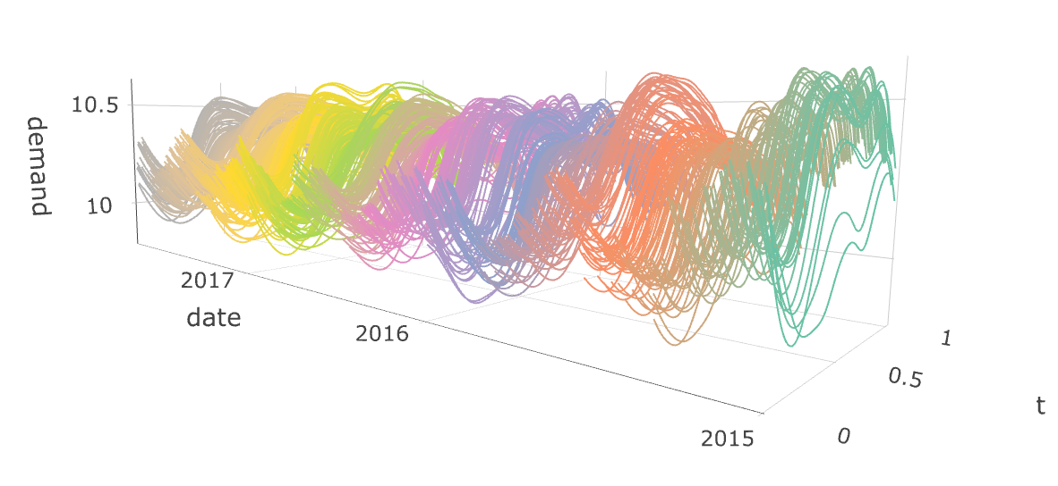
Figure 1: Functional time series plot for log-transformed electricity demand.

The original dataset are recorded by 10-minute intervals from 00:00–23:50 on each day, which consists of 144 observations. We consider the daily log-transformed real demand curves by smoothing and rescaling them to a continuous interval $[0,1]$. The plot of the smoothed functional time series is shown in Fig. 1. The stationarity test of [29] is also implemented and it turns out that the test does not reject the stationarity hypothesis at $5\%$ level during the considered period. Next, we aim to investigate the relationship between daily electricity real demand curves and future daily total demand. To this end we explore the FLM:

$$Y_{i+1}=\beta_{0}+\sum_{j=1}^{3}\int_{0}^{1}\beta_{j}(t)X_{i+1-j}(t)\mathrm{d}t+\epsilon_{i+1},\,i=3,4,...,781$$

with $Y_{i+1}$ being the daily total real demand on the $(i+1)$-th weekday.

The Legendre polynomial and FPC bases are used in this example. Firstly, we select $d_{j}=3$ by CVP criterion to explain at least 95% of the variability of the data and set $c_{j}=2d_{j}=6,~{}j=1,2,3$. The block size is chosen as $m=16$ by MV method proposed in Section 2.3 for aforementioned bases, the smoothing parameter $\lambda$ is selected as $8.5\times 10^{-12}$ based on Legendre polynomial bases and $1.7\times 10^{-11}$ based on FPC bases according to GCV criterion. The JSCBs are constructed based on 10000 bootstrap replications.

Figure 2: Estimated coefficient functions (black solid curve), $95\%$ JSCBs (blue dotdashed) and $95\%$ point-wise confidence bands (red dashed) with data-driven weights.

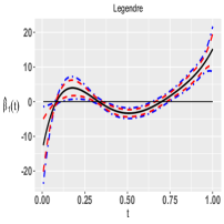
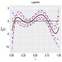
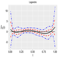
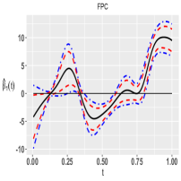
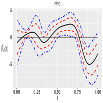
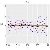
We exhibit the plots of JSCBs and point-wise confidence bands for $\beta_{1}(t),$ $\beta_{2}(t)$ and $\beta_{3}(t)$ in Fig. 2. From it, one finds that both $\beta_{1}(t)$ and $\beta_{2}(t)$ are significantly non-zero, $\beta_{3}(t)$ is insignificant under the JSCB construction for both bases. In particular, for both bases $\beta_{1}(t)$ is significantly positive at the morning and evening peak times, significantly negative at off-peak time. While $\beta_{2}(t)$ is only significantly positive in the afternoon period and significantly negative in the late evening period, contributing to a slightly weaker impact on the response compared to $\beta_{1}(t)$. On the other hand, the point-wise confidence bands for $\beta_{3}(t)$ based on both bases do not fully cover the horizontal axis $\beta_{3}(t)\equiv 0$, which will lead to a spurious significance. These findings illustrate that, the electricity demand behavior over the last two weekdays (especially the peak time from the last weekday) is highly correlated with the total demand of the next weekday. Moreover according to the the JSCB fluctuations for the coefficients $\beta_{1}(t)$ and $\beta_{2}(t)$, it turns out apparently that the constancy and linearity coefficient hypotheses are rejected.

For a further investigation, we fit the model $Y_{i+1}=\beta_{0}+\sum_{j=1}^{2}\int_{0}^{1}\beta_{j}(t)X_{i+1-j}(t)\mathrm{d}t+\epsilon_{i+1}$ and find that the $R^{2}$ of the regression is 0.8032 (0.8044) for the Legendre polynomial (FPC) bases. Therefore, we conclude that the majority of the variability of the total weekday electricity demand in Spain can be explained/predicted by the demand curves of the past two weekdays.

6 Discussions

We would like to conclude this article by discussing some issues related to the practical implementation of the regression as well as possible extensions. Firstly, the predictors $\bm{X}_{i}(t)$ are typically only discretely observed with noises in practice and hence pre-smoothing is required to transfer the discretely observed predictors into continuous curves which inevitably produces some smoothing errors. In this article, for the purposes of brevity and keeping the discussions on the main focus, we assume that the smooth curves of $\bm{X}_{i}(t)$ are observed. It can be seen from the proofs that the results of the paper hold under the densely observed functional data scenario as long as the smoothing error is of the order $O_{\mathbb{P}}(\log n/\sqrt{n})$ uniformly. The smoothing effects for time series or densely observed functional data have been intensively investigated in the literature; see for instance [23], [61] and [59], among many others. Though the aforementioned references are not exactly intended for functional time series, their results can be extended to the functional time series setting which we will pursue in a separate future work. On the other hand, we do not expect that our theory and methodology will directly carry over to the sparsely observed functional data setting ([60]) and the corresponding investigations are beyond the scope of the current paper.

Secondly, we note that the choice of the basis function is a non-trivial task in practice. In the literature, there are several discussions with respect to the choices of basis functions or methods for the regression (1) in general. See for instance Section 6.1 in [46] and the references therein. Here we shall add some additional notes. For functional time series whose observation curves are clearly periodic such as the yearly temperature curves, the Fourier basis is a natural choice. Similar choices can be made based on prior knowledge of the shapes of the observation curves in various scenarios. From our limited simulation studies and data analysis in Sections 4 and 5, it is found that many popular classes of basis functions produce similar estimates of the regression curves and inference results, which demonstrates a certain level of robustness towards the basis choices.

Finally, in some real data applications the response time series may be function-valued as well. One prominent example is the functional auto-regression [6]. We hope that our multiplier bootstrap methodology as well as the underlying Gaussian approximation and comparison results will shed light on the simultaneous inference problem for FLM with functional responses. Indeed, using the basis decomposition technique, FLM with functional responses could be viewed as multiple FLMs with scalar responses at the basis expansion coefficient level where the regression errors may be cross-correlated and the set of regressors are identical. We will investigate this direction in a future research endeavor.

References

- Aneiros et al. [2016] Aneiros, G., J. Vilar, and P. Raña (2016). Short-term forecast of daily curves of electricity demand and price. Electrical Power & Energy Systems 80, 96–108.
- Aue et al. [2017] Aue, A., L. Horváth, and D. F. Pellatt (2017). Functional generalized autoregressive conditional heteroskedasticity. Journal of Time Series Analysis 38(1), 3–21.
- Aue et al. [2015] Aue, A., D. D. Norinho, and S. Hörmann (2015). On the prediction of stationary functional time series. Journal of the American Statistical Association 110, 378–392.
- Belloni et al. [2015] Belloni, A., V. Chernozhukov, D. Chetverikov, and K. Kato (2015). Some new asymptotic theory for least squares series: Pointwise and uniform results. Journal of Econometrics 186(2), 345–366.
- Bentkus [2003] Bentkus, V. (2003). On the dependence of the Berry–Esseen bound on dimension. Journal of Statistical Planning and Inference 113(2), 385–402.
- Bosq [2012] Bosq, D. (2012). Linear Processes in Function Spaces: Theory and Applications, Volume 149. Springer Science & Business Media.
- Cai and Hall [2006] Cai, T. T. and P. Hall (2006). Prediction in functional linear regression. The Annals of Statistics 34(5), 2159–2179.
- Cardot et al. [2003] Cardot, H., F. Ferraty, and P. Sarda (2003). Spline estimators for the functional linear model. Statistica Sinica 13(3), 571–591.
- Cardot and Sarda [2011] Cardot, H. and P. Sarda (2011). Functional linear regression. In The Oxford Handbook of Functional Data Analysis. Oxford University Press.
- Chatterjee and Bose [2005] Chatterjee, S. and A. Bose (2005). Generalized bootstrap for estimating equations. The Annals of Statistics 33(1), 414–436.
- Chen [2007] Chen, X. (2007). Large sample sieve estimation of semi-nonparametric models. Handbook of Econometrics 6(B), 5549–5632.
- Chernozhukov et al. [2013] Chernozhukov, V., D. Chetverikov, and K. Kato (2013). Gaussian approximations and multiplier bootstrap for maxima of sums of high–dimensional random vectors. The Annals of Statistics 41(6), 2786–2819.
- Chernozhukov et al. [2015] Chernozhukov, V., D. Chetverikov, and K. Kato (2015). Comparison and anti-concentration bounds for maxima of gaussian random vectors. Probability Theory and Related Fields 162(1), 47–70.
- Chernozhukov et al. [2017] Chernozhukov, V., D. Chetverikov, and K. Kato (2017). Central limit theorems and bootstrap in high dimensions. The Annals of Probability 45(4), 2309–2352.
- Christophe and Sarda [2009] Christophe, Crambes., A. K. and P. Sarda (2009). Smoothing splines estimators for functional linear regression. The Annals of Statistics 37(1), 35–72.
- Dette et al. [2020] Dette, H., K. Kokot, and S. Volgushev (2020). Testing relevant hypotheses in functional time series via self-normalization. Journal of the Royal Statistical Society: Series B: Statistical Methodology 82, 629–660.
- Dette and Tang [2021] Dette, H. and J. Tang (2021). Statistical inference for function-on-function linear regression. arXiv preprint arXiv:2109.13603.
- Fan and Li [2001] Fan, J. and R. Li (2001). Variable selection via nonconcave penalized likelihood and its oracle properties. Journal of the American Statistical Association 96(456), 1348–1360.
- Fang [2016] Fang, X. (2016). A multivariate CLT for bounded decomposable random vectors with the best known rate. Journal of Theoretical Probability 29(4), 1510–1523.
- Fang and Röllin [2015] Fang, X. and A. Röllin (2015). Rates of convergence for multivariate normal approximation with applications to dense graphs and doubly indexed permutation statistics. Bernoulli 21(4), 2157–2189.
- García-Portugués et al. [2014] García-Portugués, E., W. González-Manteiga, and M. Febrero-Bande (2014). A goodness-of-fit test for the functional linear model with scalar response. Journal of Computational and Graphical Statistics 23(3), 761–778.
- Hall and Horowitz [2007] Hall, P. and J. L. Horowitz (2007). Methodology and convergence rates for functional linear regression. The Annals of Statistics 35(1), 70–91.
- Hall et al. [2006] Hall, P., H.-G. Müller, and J.-L. Wang (2006). Properties of principal component methods for functional and longitudinal data analysis. The Annals of Statistics 34(3), 1493–1517.
- Hilgert et al. [2013] Hilgert, N., A. Mas, and N. Verzelen (2013). Minimax adaptive tests for the functional linear model. The Annals of Statistics 41(2), 838–869.
- Hörmann and Kidziński [2015] Hörmann, S. and Ł. Kidziński (2015). A note on estimation in Hilbertian linear models. Scandinavian Journal of Statistics 42(1), 43–62.
- Hörmann and Kokoszka [2010] Hörmann, S. and P. Kokoszka (2010). Weakly dependent functional data. The Annals of Statistics 38(3), 1845–1884.
- Horváth and Kokoszka [2012a] Horváth, L. and P. Kokoszka (2012a). Inference for Functional Data with Applications. Springer Science & Business Media.
- Horváth and Kokoszka [2012b] Horváth, L. and P. Kokoszka (2012b). A test of significance in functional quadratic regression. In Inference for Functional Data with Applications, pp. 225–232. Springer.
- Horváth et al. [2014] Horváth, L., P. Kokoszka, and G. Rice (2014). Testing stationarity of functional time series. Journal of Econometrics 179(1), 66–82.
- Imaizumi and Kato [2019] Imaizumi, M. and K. Kato (2019). A simple method to construct confidence bands in functional linear regression. Statistica Sinica 29(4), 2055–2081.
- James et al. [2009] James, G. M., J. Wang, and J. Zhu (2009). Functional linear regression that’s interpretable. The Annals of Statistics 37(5A), 2083–2108.
- Kong et al. [2016] Kong, D., A.-M. Staicu, and A. Maity (2016). Classical testing in functional linear models. Journal of Nonparametric Statistics 28(4), 813–838.
- Lei [2014] Lei, J. (2014). Adaptive global testing for functional linear models. Journal of the American Statistical Association 109(506), 624–634.
- Li and Hsing [2007] Li, Y. and T. Hsing (2007). On rates of convergence in functional linear regression. Journal of Multivariate Analysis 98(9), 1782–1804.
- Li and Hsing [2010] Li, Y. and T. Hsing (2010). Uniform convergence rates for nonparametric regression and principal component analysis in functional/longitudinal data. The Annals of Statistics 38(6), 3321–3351.
- Liu and Lin [2009] Liu, W. and Z. Lin (2009). Strong approximation for a class of stationary processes. Stochastic Processes and their Applications 119(1), 249–280.
- Ma and Kosorok [2005] Ma, S. and M. R. Kosorok (2005). Robust semiparametric M-estimation and the weighted bootstrap. Journal of Multivariate Analysis 96, 190–217.
- McLean et al. [2015] McLean, M. W., G. Hooker, and D. Ruppert (2015). Restricted likelihood ratio tests for linearity in scalar-on-function regression. Statistics and Computing 25(5), 997–1008.
- Meyer [1992] Meyer, Y. (1992). Ondelettes et operateurs I: Ondelettes. Hermann, Paris.
- Morris [2015] Morris, J. S. (2015). Functional regression. Annual Review of Statistics and Its Application 2, 321–359.
- Newey [1997] Newey, W. K. (1997). Convergence rates and asymptotic normality for series estimators. Journal of Econometrics 79(1), 147–168.
- Panaretos and Tavakoli [2013] Panaretos, V. M. and S. Tavakoli (2013). Fourier analysis of stationary time series in function space. The Annals of Statistics 41(2), 568–603.
- Paparoditis [2018] Paparoditis, E. (2018). Sieve bootstrap for functional time series. The Annals of Statistics 46(6B), 3510–3538.
- Politis and Wolf [1999] Politis, D.N., R. J. and M. Wolf (1999). Subsampling. Springer Science & Business Media.
- Ramsay and Silverman [2005] Ramsay, J. and B. Silverman (2005). Functional Data Analysis (2nd ed.). New York: Springer.
- Reiss et al. [2017] Reiss, P. T., J. Goldsmith, H. L. Shang, and R. T. Ogden (2017). Methods for scalar-on-function regression. International Statistical Review 85(2), 228–249.
- Reiss and Ogden [2007] Reiss, P. T. and R. T. Ogden (2007). Functional principal component regression and functional partial least squares. Journal of the American Statistical Association 102(479), 984–996.
- Schmitt [1992] Schmitt, B. A. (1992). Perturbation bounds for matrix square roots and pythagorean sums. Linear Algebra and its Applications 174, 215–227.
- Shang [2014] Shang, H. L. (2014). A survey of functional principal component analysis. AStA Advances in Statistical Analysis 98(2), 121–142.
- Shang and Cheng [2015] Shang, Z. and G. Cheng (2015). Nonparametric inference in generalized functional linear models. The Annals of Statistics 43(3), 1742–1773.
- Spokoiny and Zhilova [2015] Spokoiny, V. and M. Zhilova (2015). Bootstrap confidence sets under model misspecification. The Annals of Statistics 43(6), 2653–2675.
- Su et al. [2017] Su, Y.-R., C.-Z. Di, and L. Hsu (2017). Hypothesis testing in functional linear models. Biometrics 73(2), 551–561.
- Trefethen [2008] Trefethen, L. N. (2008). Is Gauss quadrature better than Clenshaw–Curtis? SIAM review 50(1), 67–87.
- Tropp [2012] Tropp, J. A. (2012). User-friendly tail bounds for sums of random matrices. Foundations of computational mathematics 12(4), 389–434.
- Wang and Xiang [2012] Wang, H. and S. Xiang (2012). On the convergence rates of Legendre approximation. Mathematics of Computation 81(278), 861–877.
- Wang et al. [2016] Wang, J.-L., J.-M. Chiou, and H.-G. Müller (2016). Functional data analysis. Annual Review of Statistics and Its Application 3, 257–295.
- Wu [1986] Wu, C.-F. J. (1986). Jackknife, bootstrap and other resampling methods in regression analysis. The Annals of Statistics 14(4), 1261–1295.
- Wu [2005] Wu, W. B. (2005). Nonlinear system theory: Another look at dependence. Proceedings of the National Academy of Sciences 102(40), 14150–14154.
- Wu and Zhao [2007] Wu, W. B. and Z. Zhao (2007). Inference of trends in time series. Journal of the Royal Statistical Society: Series B: Statistical Methodology 69(3), 391–410.
- Yao et al. [2005] Yao, F., H.-G. Müller, and J.-L. Wang (2005). Functional data analysis for sparse longitudinal data. Journal of the American Statistical Association 100(470), 577–590.
- Zhang and Chen [2007] Zhang, J.-T. and J. Chen (2007). Statistical inferences for functional data. The Annals of Statistics 35(3), 1052–1079.
- Zhang and Cheng [2018] Zhang, X. and G. Cheng (2018). Gaussian approximation for high dimensional vector under physical dependence. Bernoulli 24(4A), 2640–2675.
- Zhou [2013] Zhou, Z. (2013). Heteroscedasticity and autocorrelation robust structural change detection. Journal of the American Statistical Association 108(502), 726–740.
- Zhou and Dette [2020] Zhou, Z. and H. Dette (2020). Statistical inference for high dimensional panel functional time series. arXiv preprint arXiv:2003.05968.