Density-Aware Personalized Training for Risk Prediction in Imbalanced Medical Data

Abstract

Medical events of interest, such as mortality, often happen at a low rate in electronic medical records, as most admitted patients survive. Training models with this imbalance rate (class density discrepancy) may lead to suboptimal prediction. Traditionally this problem is addressed through ad-hoc methods such as resampling or reweighting but performance in many cases is still limited. We propose a framework for training models for this imbalance issue: 1) we first decouple the feature extraction and classification process, adjusting training batches separately for each component to mitigate bias caused by class density discrepancy; 2) we train the network with both a density-aware loss and a learnable cost matrix for misclassifications. We demonstrate our model’s improved performance in real-world medical datasets (TOPCAT and MIMIC-III) to show improved AUC-ROC, AUC-PRC, Brier Skill Score compared with the baselines in the domain.

1 Introduction

Machine learning-based medical risk prediction models continue to grow in popularity Zhang et al. (2018b); Rajkomar et al. (2018); Miotto et al. (2016). However, the performance of these models is often biased in evaluation by commonly reported metrics (such as area under the curve of the receiver operating characteristic: AUC-ROC), often reporting overly-optimistic findings as a result of the imbalance between those that observe medical adverse events and those that do not Swets (1979); Lobo et al. (2008); Cook (2007); Huang et al. (2021). The adverse event of interest is often in the minority class Li et al. (2010). For example, in mortality prediction, patients with higher risk represent a smaller fraction in the cohort compared to most of the people who survive. Naively applying machine learning models may render dissatisfaction: the outcome of interest can be extremely costly, either through unnecessary medical intervention (type 1 error) or misdiagnosis (type 2 error). Furthermore, it is important not only to rank expired patients higher than survived patients w.r.t. probability output (e.g. AUC-ROC), but also the probability output is more calibrated Park and Ho (2020).

While methods to tackle this imbalance issue via resampling or reweighting methods constitute a popular approach Wang et al. (2020); Babar and Ade (2016), their applications in the context of medical data are often heuristic (or case by case) in nature. First, these techniques may give readjusted importance to the smaller class, but the weighting ratio remains ad-hoc from dataset to dataset, therefore, manual tuning might not be ideal. Second, apart from inter-class density discrepancy, one unique aspect of medical data is that even in the same risk group (same label), the patients may have different underlying comorbidities or risk factor characteristics that arrive at potentially high risk for various reasons, rendering intra-class heterogeneity Huo et al. (2019). This heterogeneity requires models to have a personalized training regime to distinguish the nuanced differences Huo et al. (2021), to address the imbalance in a standardized/automated fashion. Rather than treating imbalanced densities as a problem, exploiting this information in training may enhance performance Ali et al. (2013).

We propose a framework to address class imbalance density and make use of this imbalance to render density-aware training for improved risk prediction performance. First, we decouple the training of representation learning and classification. Traditionally, representation learning and classification are trained jointly Kang et al. (2019), but by decoupling, class-specific features are extracted and class-specific predictions made, removing a source of bias for the learned classifier Zhou et al. (2020). Second, the density differences are important to learn, not eliminate, when modeling. Patients with lower risk (majority) are often lower risk because they do not contain any of the common risk factors (e.g. lack of hypertension, diabetes, prior myocardial infarction), and hence, form a dense cluster. However, patients with higher risk (minority) may arrive at this high risk from different factors (e.g. renal failure versus respiratory distress), thus being scattered in the data space Huo et al. (2021). Our approach is density-aware, by avoiding re-sampling or re-weighing pre-processing steps, and the decoupling approach improves risk prediction performance. We demonstrate this approach in two different medical data scenarios: a randomized clinical trial dataset and an electronic health record (observational) dataset. We show that our method can achieve high predictive performance in these imbalanced medical datasets (imbalance ratio can range from 7 $\sim$ 10) and perhaps surprisingly it can also achieve superior calibration than the baselines without an extra set of calibration data.

Generalizable Insights about Machine Learning in the Context of Healthcare

As sophisticated models for increasingly large medical datasets are developed and promoted, evaluation of the predicted outcomes, through the use of an appropriate set of metrics is necessary. Medical data often contains low event rates for the major adverse events of interest. The primary measures of their performance, either threshold specific-based classification techniques, which may not properly account for the different costs of Type I and Type II errors, or the ability of the model to discriminate those at risk and those not, through the AUC-ROC, become overconfident in telling clinicians using the model who is not at risk. By leveraging the imbalance in the classes modeled, we are able to more accurately estimate those at risk, by more accurately identifying driving risk factors in the groups independently. As a result, this allows us to more concretely evaluate why they individuals are at risk (rather than simply being not at low-risk), and provide for better model calibration for medical decision making - through probabilistic interpretation of an occurrence in a frequentist perspective.

2 Related Work

Supervised learning methods on imbalance dataset tasks often re-balance data via re-sampling, such as oversampling Pouyanfar et al. (2018), undersampling He and Garcia (2009) classes. Others use synthetic samples to account for imbalance, where new samples are generated from perturbations of old samples Chawla et al. (2002); Zhang et al. (2018a). Another common approach is via re-weighting, which re-assigns training weights for each class based on criteria such as number of instances of each class Huang et al. (2019), effective numbers Cui et al. (2019) or the distance between loss Cao et al. (2019). However it is not clear the clinical utility of these methods since they were developed in non-medical datasets.

Medical models often focus on risk of adverse event estimation, which intrinsically carries data imbalance. Re-sampling has been widely applied Chawla et al. (2002); Bhattacharya et al. (2017). Cost-sensitive training is also applied, for example on Intensive Care Unit (ICU) data Rahman and Davis (2013). Hybrid approaches, which combine re-sampling and cost-sensitive training have also been applied Li et al. (2010). These methods all are based upon the ad hoc tuning, weighting, or re-sampling to address imbalance, but do not learn from the imbalance information itself.

Furthermore, the imbalance issue in medical dataset not only affects the prediction, but also calibration Park and Ho (2020). The currently used metrics in medical modeling are usually not geared towards calibration and the metrics most widely used, such as AUC-ROC is susceptible to imbalance ratio Huang et al. (2021). The modern-day neural networks have achieved astonishing accuracy but studies have shown most methods are getting less and less calibrated Guo et al. (2017). Therefore we will demonstrate in our model the calibration is an extra contribution on top of handling imbalance prediction

3 Methods

In this section, we introduce our framework. The approach first separates the training data to different risk groups. Then, it uses a density-aware loss function to take into account the data density difference between majority class and minority class. Finally, it uses a learnable cost matrix to personalize misclassification. We stress that our framework is a training regime that can apply to different backbones (e.g. different neural network architectures) and we will later show in experiments this framework being used on real-world tabular as well as time-series medical data. The overall pipeline is shown in Fig 1.

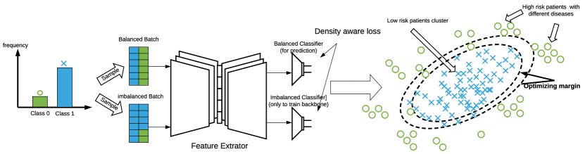
Figure 1: Overall pipeline. The original medical dataset is sampled with two distributions, one balanced and one imbalanced (default) batch. Both of the batches will go through the backbone but the classifiers will utilize different batches to optimize the density-aware loss, rendering personalized decision boundaries for different classes.

3.1 Decoupling training for imbalance classes

In neural networks, we can coarsely define the last layer (or last few layers) (Zhou et al., 2020) as the output classifier, since the output is used to determine the class of one specific instance. The previous layers of the network architecture can be deemed as the feature extractors or backbone. Traditionally these two parts are trained jointly and the distinctions between them are ill-defined (Kang et al., 2019). However, Zhou et al. (2020) showed that the classifier portion of the network is more susceptible to data imbalance, whereas the feature extractor is not, during training. Thus, we decouple training of the feature extractor and classifier.

Formally, let $\mathcal{I}=\{I_{i}\}$ be a set of inputs, and $\mathcal{Y}=\{y_{i}\}$ be the set of corresponding labels. For a typical objective function, we write:

$$\mathcal{L}=\frac{1}{N}\sum_{c=1}^{|C|}\sum_{i=1}^{|N_{c}|}l(h(I_{ci}),y_{ci}),$$ (1)

where $l(\cdot)$ is the loss function and $h(\cdot)$ is our model. $|C|$ signifies the number of total classes and $|N_{c}|$ the number of instances in one specific class. In an imbalance setting, the larger class with more training instances $|N_{c}|$ will dominate the loss and thus make the model biased. A naive way to tackle this issue is to adjust the sampling rate for the smaller class. For example, a class-balanced sampling (CBS) is proposed (Huang et al., 2016), where the instances from each class are sampled with equal probability so that the big class would not dominate the loss calculation and hence the density discrepancy will have much less effect. However, the CBS strategy will likely induce the ill-fitting problem because either the big class is under-sampled, inducing loss of information or small class is over-sampled, inducing over-fitting (Yang and Xu, 2020). We propose that for a well-trained neural network, a set of abundant and diverse training instances is required, so that the model can generalize well in the testing set. A method is required to make use of the rich information in the big class but to ensure the smaller class is well represented as well.

Inspired by Zhang et al. (2019), we are proposing a solution to use both class-balanced sampling and regular random sampling, where the first would sample each instance to make sure each class has equal probability and the latter one samples each instance with equal probability. The function can be defined:

$$p_{j}=\frac{n_{j}^{q}}{\sum_{c=1}^{|C|}n_{c}^{q}},$$ (2)

where $p_{j}$ indicates the probability of sampling a data point from class $j$ and the range for $q\in[0,1]$ and $|C|$ is the number of classes. The regular random sampling entails the $q=1$, meaning the probability will be proportional to the cardinality of the class $j$. The class-balanced sampling would entail $q=0$ which means $p_{j}=1/|C|$, and therefore each class is balanced. These two sampling strategies will generate two sets of batches, with each class’s density built in, and we will train the feature extractor with both batches while the classifier will only train on the corresponding batch. In this way the rich information of big class will be preserved and at the same time the balanced classifier, which is eventually used for prediction during inference, will not be biased towards one class.

3.1.1 Density-aware outlier detection loss

To further make use of the inherent density information among the classes, we will introduce the density-aware training. There have been many cost-sensitive methods proposed to address the imbalance issue. One of the most popular ones is the focal loss (Lin et al., 2017). This method focuses on the ‘difficult’ examples, which means the predicted probability of the example is far away from the true label. Based on previous discussion, we can treat the low risk patient as in-distribution data and high risk patients (with different underlying factors) as out-of-distribution data, and use the outlier detection technique to optimize the boundary (Huo et al., 2020).

By following this direction we propose a hinge loss based objective function. Hinge loss itself is less susceptible to density discrepancy among classes because it aims to optimize around support vectors, thus focusing the ‘difficult’ examples which are close to the decision boundary. However the traditional ‘max-margin’ training using the hinge loss did not take into account the class-wise density, which renders a non-personalized training. Our proposed personalized training is through a density-aware margin optimization (Cao et al., 2019). This Density-Aware Hinge (DAH) loss can be written as follows:

$$\mathcal{L}_{DAH} =\frac{1}{N}\sum_{c}^{|C|}\max(\max_{j\neq c}\{z_{j}\}-z_{c}+\Delta_{c},0)$$ (3)

where $$\Delta_{c}=\frac{\text{K}}{|N_{c}|^{1/4}}\text{, for}\ c\in\{1,...,|C|\},$$

where $\mathcal{L}_{DAH}$ is the density-aware hinge loss, $z_{j}$ is the model $j$-th element in the output vector, indicating the probability of this instance predicted to be $j$-th class, and $z_{c}$ is the predicted output probability of the true class $c$. The form follows the traditional hinge loss, except the density-aware component $\Delta_{c}$. The parameter K is a hyper-parameter, and $|N_{c}|$ is number of examples in class $c$. In Cao et al. (2019), the exponential in $|N_{c}|^{1/4}$ is derived by the trade-off of optimizing all the margins between classes, so that the imbalanced test error can be smaller than a generalization error bound (Wei and Ma, 2019). That is, $\gamma_{j}\propto|N_{c}|^{1/4}$, where $\gamma_{c}$ is the margin in the hyper-plane for class $c$. Therefore we follow this tuning. The hyper-parameter K is usually tuned by normalizing the last hidden activation and last fully-connected layer’s weight vectors’ $\ell_{2}$ norm to 1, as noted in Wang et al. (2018).

In practice, the hinge loss may pose difficulty for optimization due to its non-smoothness (Luo et al., 2021). First we derive the softmax from the original form and thus a relaxed form of hinge loss for smoothness is adopted to simulate the cross-entropy form:

$$\mathcal{L}_{DAH} =\frac{1}{N}\sum_{c}^{|C|}-\log\sigma(z_{c}),$$ (4)

where $$\sigma(z_{c})=\frac{\text{exp}(z_{c}-\Delta_{c})}{\text{exp}(z_{c}-\Delta_{c})+\sum_{j\neq c}\text{exp}(z_{j})},\text{and }\Delta_{c}=\frac{\text{K}}{|N_{c}|^{1/4}}\text{, for}\ c\in\{1,...,|C|\}$$

The ‘max-margin’ form is relaxed to a softmax function in the cross-entropy-like optimization. While some previous work (Liu et al., 2016; Wang et al., 2018) adopted similar ideas, our proposed personalized margin $\Delta_{c}$ can make use of the information in density discrepancy itself for training.

Table 1: A typical cost matrix where the diagonal has zero cost, and $C_{FN}$, $C_{FP}$ represents false negative cost and false positive cost, respectively.

Cost Matrix	Predicted as Positive	Predicted as Negative
True Positive	0	$C_{FN}$
True Negative	$C_{FP}$	0

3.1.2 Trainable cost matrix

For personalized training, we propose to equip the density-aware loss with a trainable cost matrix. Traditionally the cost of training has been set static throughout the whole training process (e.g. false positive cost and false negative cost in binary classification). The default cost matrix can be seen as table 1, where the $C_{FN}$, $C_{FP}$ were traditionally set to 1 (Note that the cost matrix here can only be applied to binary prediction). However this implies that the two types of cost are equal throughout the whole training (Roychoudhury et al., 2017). But as we discussed before, the big class and small class would make the model more biased towards one versus the other due to the density disparity. But we want to use some mechanism to rebalance the training so that the model would be less biased. Thus instead of treating the costs as a prior knowledge, we make them as trainable parameters along with the model as well (Fernández et al., 2018, page. 66). In this way, the model will dynamically learn the cost to minimize the loss function. For an input and target pair $(x,y)$, where the output of the model is $z=h(x)$, the loss function with incorporation of two costs under binary classification is proposed:

$$\mathcal{L}((x,y);h(\cdot))= -y\log\sigma(C_{FN}z_{\max})-(1-y)\log(1-\sigma(C_{FP}z_{\max}))$$ (5)

subject to $$C_{FN}>0,C_{FP}>0,C_{FN}>\theta C_{FP}$$

The $z_{\max}$ indicates the largest logit along the output vector. The constraints above ensure that the two types of misclassification cost will always be positive (Roychoudhury et al., 2017) and due to the minority class is the prediction of interest (such as higher risk patients), we penalize more in the event of false negatives verse false positives. Here, $\theta$ can be tuned as a hyper-parameter.

In practice, when applying stochastic gradient descent (SGD), the parameters can only be updated without constraints. Here we relax the constrained problem as an unconstrained one, we thus rewrite:

$$C_{FN}=\theta C_{FP}+\mathcal{D},$$ (6)

where $\mathcal{D}$ is a regularization term. Therefore we will only need to make sure $C_{FP}>0$ during training. We propose to minimize the objective loss function in terms of $\log C_{FP}$ instead of $C_{FP}$:

$$\frac{\partial\mathcal{L}((x,y);h(\cdot))}{\partial\log C_{FP}}=C_{FP}\frac{\partial\mathcal{L}((x,y);h(\cdot))}{\partial C_{FP}},$$ (7)

where the loss function can take the form as we defined above for density-aware training. Note that there are generally two ways to handle the constraints for optimization: reparameterization to an unconstrained minimization problem or projected gradient (PG) (Amid and Warmuth, 2020). PG is to perform unconstrained gradient updates, then project back onto the feasible space after each update. PG directly solves the convex optimization problem, but the intermediate iterates can sometimes lead to a possibly less stable or too aggressive trajectory (Raskutti and Mukherjee, 2014). Ours is similar to reparameterization where numerical stability is more warranted in this regard.

Table 2: Summary of the datasets and the tasks

Dataset	task	#instances	#features	IR
TOPCAT	Mortality	1,767	86	7.92
	hospitalization			1.71
MIMIC-III	Mortality	21,139	34	7.57
	Phenotyping			10.32

4 Experiments

4.1 Datasets

In our experiment, we test our proposed model on two real-world medical datasets which include inherent imbalance issues and heterogeneous patients representations.

1) The first dataset is TOPCAT (Treatment of Preserved Cardiac Function Heart Failure with an Aldosterone Antagonist). TOPCAT is a multi-center, international, randomized, double-blind, placebo controlled trial sponsored by the U.S. National Heart, Lung, and Blood Institute Bertram et al. (2014). TOPCAT collects patients from the United States, Canada, Brazil, Argentina, Russia, and Georgia between 2006 and 2013. The outcomes of interest were all-cause mortality and heart failure hospitalization through 3 years of follow-up. The data includes demographic and clinical data available from patients in addition to laboratory data, electrocardiography data, Kansas City Cardiomyopathy Questionnaire (KCCQ) scores (physical limitation score, symptom stability score, symptom frequency score, symptom burden score, total symptom score, self-efficacy score, quality of life score, social limitation score, overall summary score, and clinical summary score). The details of the variables are listed in supplementary Table LABEL:tab:TOPCAT_variables.

2) The second dataset is MIMIC-III (Medical Information Mart for Intensive Care). MIMIC-III is one of the largest clinical datasets that has been made publicly available Johnson et al. (2016). It contains multivariate time-series data from over 40,000 intensive care unit (ICU) stays. The types of data range from static demographics such as gender and age to rapidly changing measurements such as heart rate and arterial blood pressure. The heterogeneity is one of the major challenges when analyzing this dataset, due to the diverse patient health conditions, rapidly changing hazard ratio as well as the corresponding treatments. We focus on using only the first 48 hours after ICU admission for the prediction of patient mortality and phenotyping. The intuition is that for early risk prognosis and phenotyping, the precaution procedure can be undertaken since the average ICU stay can be up to 100 to 200 hours Johnson et al. (2016). We adopted the same data pre-processing steps as in a set of benchmark models in MIMIC-III Harutyunyan et al. (2019)(i.e. imputation, normalization, data masking, etc), where we used the same 17 clinical measurements and their derivations to construct in total 34 time-series features.

A summary of the datasets with the imbalance ratio (IR) is shown in Table 2. We test our model on three binary classifications (2 from TOPCAT, 1 from MIMIC-III) tasks and a multi-class classification task (MIMIC-III) to demonstrate our model can work under a variety of scenarios. Note that only the phenotyping task in MIMIC-III is a multi-class multi-label scenario, so the imbalance ratio is calculated between the largest class and smallest class. The listing of phenotype labels used is in supplementary Table LABEL:MIMIC_pheno, along with their medical type to indicate this is a heterogeneous set of labels that have many underlying driving factors. The model is not trained on a learnable cost matrix for phenotyping since the false positive and false negative is for binary classification, therefore, we solely rely on decoupling training and density aware loss.

4.2 Experimental Setup

For each of the datasets and tasks, we selected strong baselines from existing benchmarks.

1) Baselines for TOPCAT:

• RF Angraal et al. (2020): a Random Forest based method which is originally tested on TOPCAT dataset

• U-RF Arafat et al. (2017): a balanced Random Forest that randomly under-samples each boostrap sample to balance training

• R-MLP Babar and Ade (2016): a Multi-layer Perceptron (MLP) model that uses reweighting in the training

For all the baseline with resampling or reweighting, we train the network on 80% of the data and tune the hyper-parameters including the weighting ratio in 10% of the data, and test on the rest 10%. For our model to have a strong neural work backbone, we construct a multi-layer Perceptron model as our backbone. The construction of the backbone is similar to R-MLP Babar and Ade (2016), training the neural network with 200 epochs, with learning as 0.001 and batch size as 64. More specifically this is a 4-layer fully connected NN, the first input layer is the same as number of features and each hidden layer has 28 neurons with one residual skip connection block and output layer has 2 neuron which is later measured on cross-entropy loss. We have our model train with our proposed decoupling and density aware loss, whereas R-MLP has under-sampling as their technique with some stochastic measures.

2) Baselines for MIMIC-III:

• GRU-D Che et al. (2018): a Gated Recurrent Unit (GRU) based method where the model has a trainable decay component

• bi-LSTM Harutyunyan et al. (2019): a bi-directional Long Short-term Memory (LSTM) based method with channel-wise feature fusion

• flexEHR Deasy et al. (2019): a GRU based method that uses word embedding technique to extract features.

• GRU-U Wang et al. (2020): a GRU based method that utilizes both trainable decay and undersampling technique for imbalance handling

• c-LSTM Harutyunyan et al. (2019): a channel-wise LSTM that process each variable independently in the first layer then fuse them in the second layer

• Deep Supervision Lipton et al. (2015): an RNN based model that uses target replication for the supervision of LSTM in each time stamp, and with changing loss function the model needed to predict replicated target variables along with outcome

For the MIMIC-III dataset, we follow the same 80/10/10 splits. And we construct our backbone same as flexEHR Deasy et al. (2019) which is a GRU based method. We trained the models with 50 epochs with an early stopping threshold of 5 epochs with no increase in AUC-ROC on the validation set. The batch size is 128 and Adam optimizer is used with learning rate 0.001.

In addition to the traditional way of measuring probabilistic output of the medical models, i.e. area under the receiver operating curve (AUC-ROC), we argue that we need to incorporate the metrics that can represent the difficulties induced by imbalanced class densities. First AUC-ROC only measures the true positives (TP) and false positive (FP) relationship, which can present an overly optimistic view of an algorithm’s performance if there is large skew in the class distribution Davis and Goadrich (2006). On the other hand, area under precision-recall curve (AUC-PRC) can provide a more reliable interpretation under imbalance, due to the fact that they evaluate the fraction of true positives among positive predictions Saito and Rehmsmeier (2015), and the precision-recall relationship will change when the test set’s imbalance ratio changes, thus providing more sensitive evaluation Davis and Goadrich (2006). Furthermore, in a medical model, the conventional way of measuring the model is through Brier score Brier et al. (1950), which takes into consideration the calibration of the model. However, the Brier score is also susceptible to imbalance ratio Fernández et al. (2018). We propose to use Brier Skill Score (BSS) Fernández et al. (2018), where the model takes the calculated Brier score and compare it to a reference point, i.e. a scaled Brier score by its maximum score under a non-informative model Steyerberg et al. (2010), to show the improvement:

$$BSS=1-\frac{BS}{BS_{\text{max}}}$$ (8)

We chose the reference $BS_{\text{max}}$ to the the prevalence predictor to output the probability based on the imbalance ratio, i.e. $BS_{\textrm{max}}=\frac{1}{N}\sum_{t=1}^{N}(f_{t}-o_{t})^{2}$ and prediction $f_{t}$ is replaced by the event rate and $o_{t}$ is the outcome label of interest Center (2005).

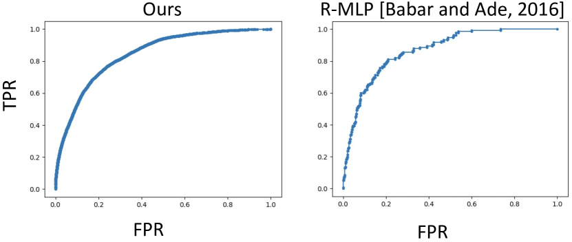
Figure 2: AUC-ROC comparison

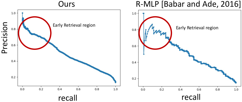
Figure 3: AUC-PRC comparison

Table 3: Results for TOPCAT dataset

Task	Methods	AUC-ROC	AUC-PRC	BSS
Mortality	RF Angraal et al. (2020)	0.723 $\pm$ 0.003	0.512 $\pm$ 0.001	-0.357 $\pm$ 0.002
	U-RF Arafat et al. (2017)	0.752 $\pm$ 0.002	0.532 $\pm$ 0.002	-0.103 $\pm$ 0.003
	R-MLP Babar and Ade (2016)	0.736 $\pm$ 0.001	0.523 $\pm$ 0.005	-0.067 $\pm$ 0.003
	Ours	0.794 $\pm$ 0.002	0.583 $\pm$ 0.002	0.166 $\pm$ 0.003
Hospitalization	RF Angraal et al. (2020)	0.763 $\pm$ 0.005	0.657 $\pm$ 0.006	-0.008 $\pm$ 0.0004
	U-RF Arafat et al. (2017)	0.771 $\pm$ 0.005	0.674 $\pm$ 0.006	-0.005 $\pm$ 0.003
	R-MLP Babar and Ade (2016)	0.789 $\pm$ 0.003	0.661 $\pm$ 0.005	-0.012 $\pm$ 0.001
	Ours	0.788 $\pm$ 0.007	0.711 $\pm$ 0.003	0.132 $\pm$ 0.002

Table 4: Results for MIMIC-III dataset

Task	Methods	AUC-ROC	AUC-PRC	BSS
Mortality	GRU-D Che et al. (2018)	0.852 $\pm$ 0.002	-	-
	bi-LSTM Harutyunyan et al. (2019)	0.862 $\pm$ 0.004	0.515 $\pm$ 0.001	-0.801 $\pm$ 0.002
	flexEHR Deasy et al. (2019)	0.878 $\pm$ 0.004	0.513 $\pm$ 0.002	-1.105 $\pm$ 0.003
	GRU-U Wang et al. (2020)	0.876 $\pm$ 0.006	0.532 $\pm$ 0.002	-
	Ours	0.892 $\pm$ 0.001	0.586$\pm$ 0.004	0.240 $\pm$ 0.003

Task	Methods	Macro AUC-ROC	Micro AUC-ROC
Phenotyping	c-LSTM Harutyunyan et al. (2019)	0.708 $\pm$ 0.0023	0.725 $\pm$ 0.0053
	bi-LSTM Harutyunyan et al. (2019)	0.770 $\pm$ 0.0081	0.791 $\pm$ 0.0048
(Multi-class,	flexEHR Deasy et al. (2019)	0.755 $\pm$ 0.0052	0.814 $\pm$ 0.0071
Multi-label)	Deep Supervision Lipton et al. (2015)	0.679 $\pm$ 0.0074	0.713 $\pm$ 0.0061
	Ours	0.771 $\pm$ 0.0061	0.821 $\pm$ 0.0049

4.3 Results

First, for the TOPCAT dataset in Table 3, we have compared our model with the baselines and we repeated the experiments in a 5-fold cross-validation scenario and compute the 95% confidence intervals. In the mortality prediction task, we are performing better on three metrics, especially in the imbalance oriented metric, AUC-PRC and BSS. The margin improved on AUC-PRC is obvious, showing the model is sensitive on finding a balance between precision and recall, both of which measure the performance of the class of interest (minority class where the patients eventually expired). Furthermore, the baselines model all have negative BSS scores, showing that in this mortality prediction scenario, the imbalance can pose a big challenge for a model to calibrate. In fact negative BSS is not uncommon in existing work Weigel et al. (2007); Leadbetter et al. (2022), showing that many modern-day models can have high predictive power but are poor at calibration, as noted in Guo et al. (2017). We will later show that by comparing against with some post hoc calibration technique on the baselines, our model can still stand out on both prediction and calibration. Next for hospitalization prediction, our model also outperforms the baselines in two of the key metrics. The AUC-ROC is second to the best, after the same model backbone trained on resampling. We suspect this is due to the fact that the IR score is lower in this task, rendering less focus on difficulty induced by imbalance and resampling is designed to handle the example-wise difficulty. However as we discussed before, the AUC-ROC is not sensitive to class distribution so the majority class’s performance can lead to the model having an overly optimistic evaluation. We compared the AUC-ROC plot and AUC-PRC plot of our model and the R-MLP baseline in Figure 3 and 3. As can be seen, the AUC-ROC plots of the two models are similar, however, the AUC-PRC plot shows on the upper region of the curve the baseline is performing rather unstably but our model gives a more smooth curve. In Saito and Rehmsmeier (2015), this region is defined as early retrieval region, where is usually used to measure in information retrieval application for when results of interest account for a small portion of all the corpus Hilden (1991); Truchon and Bayly (2007) (what is the model precision when recall rate is low). We can conclude our model has better performance on AUC-PRC is due to the better part on early retrieval where it can better handle the imbalance for the class of interest.

For the MIMIC-III dataset in Table 4, we also compared our model with the baselines (Note some metrics are empty due to the original model did not report those metrics and there is no publicly available code to replicate the results). First, for mortality prediction, our model is again better across the board among all the three metrics, especially on BSS evaluation on the model. It is perhaps surprising that traditional medical models were rarely optimized w.r.t. calibration, which however is an important metric for medicine Van Calster et al. (2019). For the phenotyping task, due to multi-class, multi-label scenario, the previously existing methods did not adopt AUC-PRC (precision, recall are used mostly in binary classification) or BSS (Brier score is used in a 1-0 probabilistic output model for calibration purposes.) So we instead use macro AUC-ROC and micro AUC-ROC for model performance comparison. From the table, we can see our model is better than all the baselines on these two metrics, showing the multi-class multi-label imbalance scenario can also be handled by our framework.

Table 5: Calibration study for TOPCAT dataset

Methods	AUC-ROC	AUC-PRC	BSS
RF Angraal et al. (2020)	0.723 $\pm$ 0.003	0.512 $\pm$ 0.001	-0.357 $\pm$ 0.002
w/ Califorest Park and Ho (2020)	0.734 $\pm$ 0.003	0.498 $\pm$ 0.001	-0.052 $\pm$ 0.002
R-MLP Babar and Ade (2016)	0.736 $\pm$ 0.001	0.523 $\pm$ 0.005	-0.067 $\pm$ 0.003
w/ Temperature scaling Guo et al. (2017)	0.744 $\pm$ 0.003	0.518 $\pm$ 0.001	0.102 $\pm$ 0.002
Ours	0.794 $\pm$ 0.002	0.583 $\pm$ 0.002	0.166 $\pm$ 0.003

In Guo et al. (2017), the authors argued the confidence calibration, being the problem of predicting probability estimates representative of the true correctness likelihood, is important for classification models in many applications, but modern neural networks are becoming increasingly lacking in this respect. They proposed a temperature scaling method to calibrate the model which is a variant of Platt scaling Platt et al. (1999). The method is to use sigmoid function as the transformation for model’s output into proper posterior probability. Our method of distribution-aware loss resembles the temperature scaling in that we have a component in the softmax to ‘soften’ the probability similarly to the temperature variable. Furthermore the component is label distribution aware, making it particularly suitable for calibration in an imbalanced setting. We aim to compare against this method. Furthermore, the tree-based methods all performed badly especially in terms of calibration. We will use a calibration specifically designed for tree models, i.e. Califorest Park and Ho (2020), where the authors used Out-of-Bag (OOB) samples as the calibration set and each individual prediction is used to calculate the weights for the samples. We will use these two methods as the post hoc calibration method (i.e. the model is calibrated after finished training, this will theoretically give them more advantage since our model does not use any post hoc calibration) for the tree-based model and neural networks to study if the BSS metric for them can be increased to positive. We did our experiment on TOPCAT dataset and the task is hospital mortality prediction. The results are shown in Table 5. As we can see we have equipped the tree model, i.e. Random Forest, the Califorest and R-MLP the Temperature scaling to calibrate after the training, which renders improvement on BSS for both of the cases. The RF has not been able to push BSS to positive but the improvement is more substantial. The temperature scaling has pushed the neural network to have postive BSS, meaning the calibration is better than a model that outputs the prevalence of the events. However we should note that both of the post hoc calibration techniques have lowered the AUC-PRC, meaning the predictive power is compromised for the calibration. In our model we can observe high predictive power as well as calibration. We postulate that the decoupling training indeed separates the bias from imbalanced data to the classifier while the feature extractor maintains the power of absorbing all information. The label distribution-aware loss, acting similarly to the Temperature scaling (where the scaling factor is inherently tuned during training with our modified softmax formulation), is calibrating the balanced classifier without sacrifice of predictive power. To this end, without using the extra calibration dataset is not an issue anymore. We have tried to test the Temperature scaling on our model but we did not observe improvement on calibration but the AUC-ROC and AUC-PRC are slightly compromised as well.

Furthermore, as a proof-of-concept, we are particularly interested if our assumption holds, i.e. the patients who survived would be similar to each other where the patients who expire would be more dissimilar. We have extracted the embedded vector from our model whose backbone is based on Deasy et al. (2019), carrying 256-dimension last hidden layer (before classifier) on the mortality prediction task in MIMIC-III. And then we apply t-SNE Linderman et al. (2019) which is a visualization algorithm to embed the data into 2 dimensions. We plot the embedding along with their labels to show the density differences, shown in Figure 4. As we can see, the survived patients account for a small and condensed space where the patients who expired would form different peaks, indicating different local clusters (e.g. diseases/phenotypes). This can prove the assumption of the density discrepancy as training information can be truly captured.

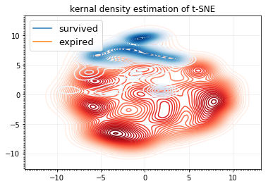
Figure 4: Density plot of survived/expired patients

Table 6: Ablation study for TOPCAT dataset

Task	Methods	AUC-ROC	AUC-PRC	BSS
Mortality	MLP	0.736 $\pm$ 0.004	0.523 $\pm$ 0.002	-0.067 $\pm$ 0.001
	MLP-TrainableCost	0.770 $\pm$ 0.003	0.541 $\pm$ 0.002	-0.188 $\pm$ 0.001
	MLP-decoupling	0.778 $\pm$ 0.002	0.569 $\pm$ 0.005	-0.480 $\pm$ 0.004
	MLP-FL	0.782 $\pm$ 0.004	0.541 $\pm$ 0.003	-0.080 $\pm$ 0.004
	MLP-DAH	0.779 $\pm$ 0.001	0.549 $\pm$ 0.005	0.111 $\pm$ 0.004
	MLP-Ours	0.798 $\pm$ 0.002	0.589 $\pm$ 0.001	0.178 $\pm$ 0.002

Table 7: Ablation study for MIMIC-III dataset

Task	Methods	AUC-ROC	AUC-PRC	BSS
Mortality	GRU	0.871 $\pm$ 0.004	0.514 $\pm$ 0.003	-1.116 $\pm$ 0.005
	GRU-TrainableCost	0.879 $\pm$ 0.001	0.520 $\pm$ 0.002	-1.108 $\pm$ 0.005
	GRU-decoupling	0.892 $\pm$ 0.003	0.577 $\pm$ 0.002	-0.909 $\pm$ 0.002
	GRU-FL	0.875 $\pm$ 0.008	0.523$\pm$ 0.007	-0.112 $\pm$ 0.007
	GRU-DAH	0.876 $\pm$ 0.003	0.534 $\pm$ 0.005	0.078 $\pm$ 0.003
	GRU-Ours	0.892$\pm$ 0.001	0.586$\pm$ 0.004	0.240$\pm$ 0.004

4.3.1 Ablation Study

We have a few components in our model such as decoupling training and density aware loss function. We are interested to know what makes the model improve and how can we dissect the model to demonstrate. We aim to study how does the decoupling help the prediction, and specifically what has the model learned. Also by comparing density aware loss with vanilla version (traditional cross-entropy loss) as well as another advanced version of loss function (focal loss Lin et al. (2017)), we conduct a thorough comparison between them. In MIMIC, we have an existing strong backbone that we can apply our techniques on Deasy et al. (2019), which is based on a GRU model. In the TOPCAT dataset, to construct a strong backbone, we make use of the same MLP architecture as in R-MLP Babar and Ade (2016) with a residual skip connection block He et al. (2016) that can be further decoupled or trained with different loss functions. We listed our ablation study in Table 6 and 7 in these two datasets both for mortality prediction.

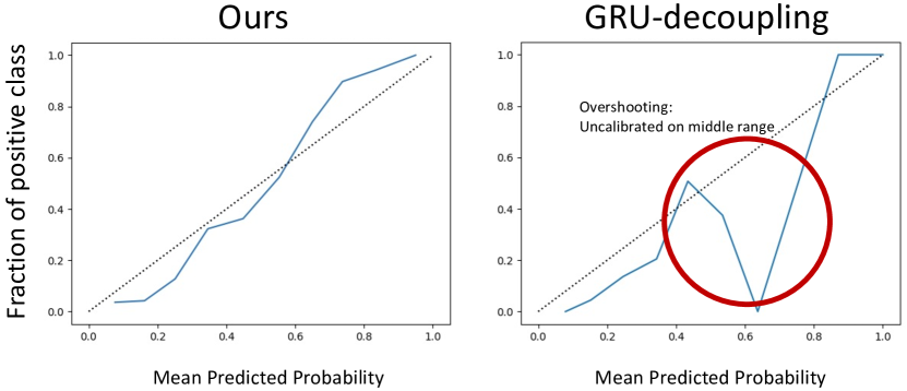
Figure 5: Calibration plot comparison

First, for the TOPCAT dataset, we can see that when fully applying our framework on the backbone, the model would outperform all other variants in Table 6. Another finding is that the decoupling training is improving the AUC-PRC in a larger margin than others, suggesting that this way of training can largely avoid the imbalance issue by through a more distribution-aware metric. However the shortcoming of decoupling alone is that it is bad at calibration, where it is among the worst BSS metric in the methods. Second, when applying density aware loss alone, we can see the model can be better calibrated (i.e. positive BSS), which is usually an important aspect of a medical model Angraal et al. (2020) because the output probability can be evaluated as the risk score for further ranking. For the MIMIC-III dataset in Table 7, we can see that the decoupling itself can improve significantly and this method alone can give good AUC-ROC (tied as best). We are then interested to know how does this single trick compare to the full framework on improving BSS in terms of calibration. The comparison is in Fig 5 where we can see our model’s calibration is closer to diagonal, rendering a more natural ‘S’ shape Fellowship and Grant (2008), where the baseline GRU-decoupling has poor calibrated range when the output probability is in mid/high range (which is the label of high-risk patients). This is showing the model is overshooting for this range of probability, likely due to an density discrepancy, because the model would assign overconfident probability to the patients in higher risk, requiring a density aware training. The over-confident prediction is prevalent in modern-day neural networks, where the mean predicted probability is higher than the fraction of positive class in a certain bin as noted in Guo et al. (2017). However, when equipped with the full framework, the performance of our model can increase significantly, especially on Brier Skill Score for calibration and rendering the plot to be closer to the diagonal (perfect calibration).

4.3.2 Parameter study

Since we have incorporated a trainable cost matrix, and we are interested in how does the parameter $\theta$ in Eq. 5 change the performance in the model. We have search on a space of $\{1,5,10,25,50,100\}$ for $\theta$, following Roychoudhury et al. (2017). On the TOPCAT dataset for mortality prediction we conduct the experiments and show it in Figure 6. We can see that AUC-ROC peaks at $\theta=5$ while AUC-PRC can be $\theta=10$. However, given the confidence interval’s overlap, the significance for choosing $\theta=10$ over $\theta=5$ for AUC-PRC can be statistically minimal, therefore $\theta=5$ is chosen.

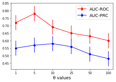
Figure 6: Tuning of $\theta$ for AUC-ROC and AUC-PRC

5 Conclusion

We proposed a framework to treat class imbalance, which is prevalent in medical datasets. The introduced framework not only addresses imbalanced class densities but also makes use of the density discrepancy to train a model. The decoupled training method alleviated bias caused by the majority class, by ensuring faithful representation of the minority class. Further, we used a density-aware loss to personalize training of each class, specifically: learning that lower-risk patients arrive at low risk by calculation of the similar factors, forming a dense cluster in the data space, but high-risk patients are dissimilar, driving them to different regions of the data space. We demonstrated that our model, trained with this decoupling framework along with density-aware loss and learnable cost matrix, outperformed baseline approaches when applied to risk prediction in medical datasets. Furthermore, through experiments we find that traditional models were poorly calibrated, calling for more comprehensive evaluation, especially geared towards imbalance issues. Our framework overall has shown to be better at prediction as well as calibration, which can be of great use in the medical domain. This project is in part supported by the Defense Advanced Research Projects Agency under grant FA8750-18-2-0027.

Appendix A.

The table of used variables for TOPCAT dataset along with their definitions

Table 8: List of Candidate Variables used for Predicting Mortality

Variable Names	Definition
age_entry.x	Age entering the study
GENDER.x	Gender of the subject
RACE_WHITE	White or Caucasian
RACE_BLACK	Race: Black
RACE_ASIAN	Race: Asian
RACE_OTHER	Race: Other
ETHNICITY	Subject of Hispanic, Latino, or Spanish origin?
DYSP_CUR	Dyspnea: Present at screening?
DYSP_YR	Dyspnea: experienced in past year?
ORT_CUR	Orthopnea: Present at screening?
ORT_YR	Orthopnea: experienced in past year?
DOE_CUR	Dyspnea on exertion: Present at screening?
DOE_YR	Dyspnea on exertion: experienced in past year?
RALES_CUR	Rales present at screening?
RALES_YR	Rales: experienced in past year?
JVP_CUR	JVP: Present at screening?
JVP_YR	JVP: experienced in past year?
EDEMA_CUR	Edema: Present at screening?
EDEMA_YR	Edema: experienced in past year?
EF	Ejection Fraction
CHF_HOSP	Previous hospitalization for CHF
chfdc_dt3	Time Between randomization and Hospitalization for Cardiac Heart Failure (years)
MI	Previous myocardial infarction
STROKE	Previous Stroke
CABG	Previous Coronary artery bypass graft surgery
PCI	Previous Percutaneous Coronary Revascularization
ANGINA	Angina Pectoris
COPD	Chronic Obstructive Pulmonary Disease
ASTHMA	Asthma
HTN	Hypertension
PAD	Peripheral Arterial Disease
DYSLIPID	Dyslipidemia
ICD	Implanted cardioverter defibrillator
PACEMAKER	Pacemaker implanted
AFIB	Atrial fibrillation
DM	Diabetes Mellitus
treat_sp_cat	Treat for diabetes mellitus: other: specify (categorical variable)
SMOKE_EVER	Has subject ever been a smoker
QUIT_YRS	How many years since quitting
alcohol4_cat	How many Drinks do you consume per week (0/1-5/5-10/11+)
HEAVY_WK	Exercise: Heavy
MED_WK	Exercise: Medium
LIGHT_WK	Exercise: Light
LIGHT_MIN	Exercise: Light: Minutes
mets per week	Activity Level (mets per week)
cooking_salt_score	Cooking Salt Score
nyha_class_cat	NYHA class 3&4 vs 1&2
HR.x	Heart rate
SBP	Systolic blood pressure
DBP	Diastolic blood pressure
gfr	Glomerular Filtration Rate
NA_mmolL	Sodium: Result (mmol/L)
K_mmolL	Potassium: Result (mmol/L)
CL_mmolL	Chloride: Result (mmol/L)
CO2_mmolL	CO2: Result (mmol/L)
BUN_mgdL	Blood Urea Nitrogen: Result (mg/dL)
GLUCOSE_mgdL	Glucose: Result (mg/dL)
GLUCOSE_INDICATOR	Whether the glucose measured was fasting or random
WBC_k/$\mu$L	WBC count: Result (k/uL)
HB_gdL	Hemoglobin: Result (g/dL)
PLT_k/$\mu$L	Platelet Count: Result (k/uL)
ALT_UL	Alanine Aminotransferase: Results (U/L)
ALP_UL	Alkaline Phosphatase: Results (U/L)
AST_UL	Aspartate Aminotransferase: Results (U/L)
TBILI_mgdL	Total Bilirubin: Results (mg/dL)
ALB_gdL	Albumin: Results (g/dL)
urine_val_mgg	Urine Microalbumin/Creatinine Ratio: Result (mg/g)
QRS_DUR	QRS Duration
ECG_AFIB	Atrial fibrillation/Flutter
ECG_BBB2	Bundle Branch Block - Yes/No indicator
ECG_VPR	Ventricular paced rhythm
ECG_Q	Pathological Q waves
ECG_LVH	Left ventricular hypertrophy
drug.x	Treatment Group (Spironolactone or Placebo)
BMI	Body Mass Index
cigpacksperday	Number of cigarettes per day
phys_limit_score	KCCQ: Physical Limitation score
symp_stab_score	KCCQ: Symptom Stability score
symp_freq_score	KCCQ: Symptom Frequency score
symp_bur_score	KCCQ: Symptom Burden score
tot_symp_score	KCCQ: Total Symptom score
self_eff_score	KCCQ: Self-Efficacy score
qol_score	KCCQ: Quality of Life score
soc_limit_score	KCCQ: Social Limitation score
overall_sum_score	KCCQ: Overall Summary score
clin_sum_score	KCCQ: Clinical Summary score

Table 9: Phenotype labels for MIMIC-III dataset

Phenotype	type
Acute and unspecified renal failure	acute
Essential hypertension	chronic
Acute cerebrovascular disease	acute
Fluid and electrolyte disorders	acute
Acute myocardial infarction	acute
Gastrointestinal hemorrhage	acute
Respiratory failure; insufficiency; arrest	acute
Hypertension with complications	chronic
Chronic kidney disease	chronic
Other liver diseases	mixed
Chronic obstructive pulmonary disease	chronic
Other lower respiratory disease	acute
Complications of surgical/medical care	acute
Other upper respiratory disease	acute
Pleurisy; pneumothorax; pulmonary collapse	acute
Conduction disorders	mixed
Congestive heart failure; nonhypertensive	mixed
Pneumonia	acute
Coronary atherosclerosis and related	chronic
Cardiac dysrhythmias	mixed
Diabetes mellitus with complications	mixed
Diabetes mellitus without complication	chronic
Disorders of lipid metabolism	chronic
Septicemia (except in labor)	acute
Shock	acute

References

- Ali et al. (2013) Aida Ali, Siti Mariyam Shamsuddin, and Anca L Ralescu. Classification with class imbalance problem. Int. J. Advance Soft Compu. Appl, 5(3), 2013.
- Amid and Warmuth (2020) Ehsan Amid and Manfred KK Warmuth. Reparameterizing mirror descent as gradient descent. Advances in Neural Information Processing Systems, 33:8430–8439, 2020.
- Angraal et al. (2020) Suveen Angraal, Bobak J Mortazavi, Aakriti Gupta, Rohan Khera, Tariq Ahmad, Nihar R Desai, Daniel L Jacoby, Frederick A Masoudi, John A Spertus, and Harlan M Krumholz. Machine learning prediction of mortality and hospitalization in heart failure with preserved ejection fraction. JACC: Heart Failure, 8(1):12–21, 2020.
- Arafat et al. (2017) Md Yasir Arafat, Sabera Hoque, and Dewan Md Farid. Cluster-based under-sampling with random forest for multi-class imbalanced classification. In 2017 11th International Conference on Software, Knowledge, Information Management and Applications (SKIMA), pages 1–6. IEEE, 2017.
- Babar and Ade (2016) Varsha Babar and Roshani Ade. Mlp-based undersampling technique for imbalanced learning. In 2016 International Conference on Automatic Control and Dynamic Optimization Techniques (ICACDOT), pages 142–147. IEEE, 2016.
- Bertram et al. (2014) P Bertram et al. Spironolactone for heart failure with preserved ejection fraction. treatment of preserved cardiac function heart failure with an aldosterone antagonist (topcat trial). N Engl J Med, 370:1383–92, 2014.
- Bhattacharya et al. (2017) Sakyajit Bhattacharya, Vaibhav Rajan, and Harsh Shrivastava. Icu mortality prediction: a classification algorithm for imbalanced datasets. In Proceedings of the AAAI Conference on Artificial Intelligence, volume 31, 2017.
- Brier et al. (1950) Glenn W Brier et al. Verification of forecasts expressed in terms of probability. Monthly weather review, 78(1):1–3, 1950.
- Cao et al. (2019) Kaidi Cao, Colin Wei, Adrien Gaidon, Nikos Arechiga, and Tengyu Ma. Learning imbalanced datasets with label-distribution-aware margin loss. Advances in neural information processing systems, 32, 2019.
- Center (2005) NOAA-CIRES Climate Diagnostics Center. Brier skill scores, rocs, and economic value diagrams can report false skill. 2005.
- Chawla et al. (2002) Nitesh V Chawla, Kevin W Bowyer, Lawrence O Hall, and W Philip Kegelmeyer. Smote: synthetic minority over-sampling technique. Journal of artificial intelligence research, 16:321–357, 2002.
- Che et al. (2018) Zhengping Che, Sanjay Purushotham, Kyunghyun Cho, David Sontag, and Yan Liu. Recurrent neural networks for multivariate time series with missing values. Scientific reports, 8(1):1–12, 2018.
- Cook (2007) Nancy R Cook. Use and misuse of the receiver operating characteristic curve in risk prediction. Circulation, 115(7):928–935, 2007.
- Cui et al. (2019) Yin Cui, Menglin Jia, Tsung-Yi Lin, Yang Song, and Serge Belongie. Class-balanced loss based on effective number of samples. In Proceedings of the IEEE/CVF conference on computer vision and pattern recognition, pages 9268–9277, 2019.
- Davis and Goadrich (2006) Jesse Davis and Mark Goadrich. The relationship between precision-recall and roc curves. In Proceedings of the 23rd international conference on Machine learning, pages 233–240, 2006.
- Deasy et al. (2019) Jacob Deasy, Ari Ercole, and Pietro Liò. Impact of novel aggregation methods for flexible, time-sensitive ehr prediction without variable selection or cleaning. CoRR, abs/1909.08981, 2019. URL http://arxiv.org/abs/1909.08981.
- Fellowship and Grant (2008) NIH Postdoctoral Fellowship and NIDA Institutional Training Grant. B. jill venton, ph. d. Journal Advisory Board, 2008(2010), 2008.
- Fernández et al. (2018) Alberto Fernández, Salvador García, Mikel Galar, Ronaldo C Prati, Bartosz Krawczyk, and Francisco Herrera. Learning from imbalanced data sets, volume 10. Springer, 2018.
- Guo et al. (2017) Chuan Guo, Geoff Pleiss, Yu Sun, and Kilian Q Weinberger. On calibration of modern neural networks. In International Conference on Machine Learning, pages 1321–1330. PMLR, 2017.
- Harutyunyan et al. (2019) Hrayr Harutyunyan, Hrant Khachatrian, David C Kale, Greg Ver Steeg, and Aram Galstyan. Multitask learning and benchmarking with clinical time series data. Scientific data, 6(1):1–18, 2019.
- He and Garcia (2009) Haibo He and Edwardo A Garcia. Learning from imbalanced data. IEEE Transactions on knowledge and data engineering, 21(9):1263–1284, 2009.
- He et al. (2016) Kaiming He, Xiangyu Zhang, Shaoqing Ren, and Jian Sun. Deep residual learning for image recognition. In Proceedings of the IEEE conference on computer vision and pattern recognition, pages 770–778, 2016.
- Hilden (1991) Jørgen Hilden. The area under the roc curve and its competitors. Medical Decision Making, 11(2):95–101, 1991.
- Huang et al. (2016) Chen Huang, Yining Li, Chen Change Loy, and Xiaoou Tang. Learning deep representation for imbalanced classification. In Proceedings of the IEEE conference on computer vision and pattern recognition, pages 5375–5384, 2016.
- Huang et al. (2019) Chen Huang, Yining Li, Chen Change Loy, and Xiaoou Tang. Deep imbalanced learning for face recognition and attribute prediction. IEEE transactions on pattern analysis and machine intelligence, 42(11):2781–2794, 2019.
- Huang et al. (2021) Chenxi Huang, Shu-Xia Li, César Caraballo, Frederick A Masoudi, John S Rumsfeld, John A Spertus, Sharon-Lise T Normand, Bobak J Mortazavi, and Harlan M Krumholz. Performance metrics for the comparative analysis of clinical risk prediction models employing machine learning. Circulation: Cardiovascular Quality and Outcomes, pages CIRCOUTCOMES–120, 2021.
- Huo et al. (2019) Zepeng Huo, Harinath Sundararajhan, Nathan C Hurley, Adrian Haimovich, R Andrew Taylor, and Bobak J Mortazavi. Sparse embedding for interpretable hospital admission prediction. In 2019 41st Annual International Conference of the IEEE Engineering in Medicine and Biology Society (EMBC), pages 3438–3441. IEEE, 2019.
- Huo et al. (2020) Zepeng Huo, Arash PakBin, Xiaohan Chen, Nathan Hurley, Ye Yuan, Xiaoning Qian, Zhangyang Wang, Shuai Huang, and Bobak Mortazavi. Uncertainty quantification for deep context-aware mobile activity recognition and unknown context discovery. In International Conference on Artificial Intelligence and Statistics, pages 3894–3904. PMLR, 2020.
- Huo et al. (2021) Zepeng Huo, Lida Zhang, Rohan Khera, Shuai Huang, Xiaoning Qian, Zhangyang Wang, and Bobak J Mortazavi. Sparse gated mixture-of-experts to separate and interpret patient heterogeneity in ehr data. In 2021 IEEE EMBS International Conference on Biomedical and Health Informatics (BHI), pages 1–4. IEEE, 2021.
- Johnson et al. (2016) Alistair EW Johnson, Tom J Pollard, Lu Shen, H Lehman Li-wei, Mengling Feng, Mohammad Ghassemi, Benjamin Moody, Peter Szolovits, Leo Anthony Celi, and Roger G Mark. Mimic-iii, a freely accessible critical care database. Scientific data, 3:160035, 2016.
- Kang et al. (2019) Bingyi Kang, Saining Xie, Marcus Rohrbach, Zhicheng Yan, Albert Gordo, Jiashi Feng, and Yannis Kalantidis. Decoupling representation and classifier for long-tailed recognition. In International Conference on Learning Representations, 2019.
- Leadbetter et al. (2022) Susan J Leadbetter, Andrew R Jones, and Matthew C Hort. Assessing the value meteorological ensembles add to dispersion modelling using hypothetical releases. Atmospheric Chemistry and Physics, 22(1):577–596, 2022.
- Li et al. (2010) Der-Chiang Li, Chiao-Wen Liu, and Susan C Hu. A learning method for the class imbalance problem with medical data sets. Computers in biology and medicine, 40(5):509–518, 2010.
- Lin et al. (2017) Tsung-Yi Lin, Priya Goyal, Ross Girshick, Kaiming He, and Piotr Dollár. Focal loss for dense object detection. In Proceedings of the IEEE international conference on computer vision, pages 2980–2988, 2017.
- Linderman et al. (2019) George C Linderman, Manas Rachh, Jeremy G Hoskins, Stefan Steinerberger, and Yuval Kluger. Fast interpolation-based t-sne for improved visualization of single-cell rna-seq data. Nature methods, 16(3):243–245, 2019.
- Lipton et al. (2015) Zachary C Lipton, David C Kale, Charles Elkan, and Randall Wetzel. Learning to diagnose with lstm recurrent neural networks. arXiv preprint arXiv:1511.03677, 2015.
- Liu et al. (2016) Weiyang Liu, Yandong Wen, Zhiding Yu, and Meng Yang. Large-margin softmax loss for convolutional neural networks. In ICML, volume 2, page 7, 2016.
- Lobo et al. (2008) Jorge M Lobo, Alberto Jiménez-Valverde, and Raimundo Real. Auc: a misleading measure of the performance of predictive distribution models. Global ecology and Biogeography, 17(2):145–151, 2008.
- Luo et al. (2021) JunRu Luo, Hong Qiao, and Bo Zhang. Learning with smooth hinge losses. Neurocomputing, 463:379–387, 2021.
- Miotto et al. (2016) Riccardo Miotto, Li Li, Brian A Kidd, and Joel T Dudley. Deep patient: an unsupervised representation to predict the future of patients from the electronic health records. Scientific reports, 6(1):1–10, 2016.
- Park and Ho (2020) Yubin Park and Joyce C Ho. Califorest: calibrated random forest for health data. In Proceedings of the ACM Conference on Health, Inference, and Learning, pages 40–50, 2020.
- Platt et al. (1999) John Platt et al. Probabilistic outputs for support vector machines and comparisons to regularized likelihood methods. Advances in large margin classifiers, 10(3):61–74, 1999.
- Pouyanfar et al. (2018) Samira Pouyanfar, Yudong Tao, Anup Mohan, Haiman Tian, Ahmed S Kaseb, Kent Gauen, Ryan Dailey, Sarah Aghajanzadeh, Yung-Hsiang Lu, Shu-Ching Chen, et al. Dynamic sampling in convolutional neural networks for imbalanced data classification. In 2018 IEEE conference on multimedia information processing and retrieval (MIPR), pages 112–117. IEEE, 2018.
- Rahman and Davis (2013) M Mostafizur Rahman and Darryl N Davis. Addressing the class imbalance problem in medical datasets. International Journal of Machine Learning and Computing, 3(2):224, 2013.
- Rajkomar et al. (2018) Alvin Rajkomar, Eyal Oren, Kai Chen, Andrew M Dai, Nissan Hajaj, Michaela Hardt, Peter J Liu, Xiaobing Liu, Jake Marcus, Mimi Sun, et al. Scalable and accurate deep learning with electronic health records. NPJ Digital Medicine, 1(1):1–10, 2018.
- Raskutti and Mukherjee (2014) Garvesh Raskutti and Sayan Mukherjee. The information geometry of mirror descent. stat, 1050:29, 2014.
- Roychoudhury et al. (2017) Shoumik Roychoudhury, Mohamed Ghalwash, and Zoran Obradovic. Cost sensitive time-series classification. In Joint European Conference on Machine Learning and Knowledge Discovery in Databases, pages 495–511. Springer, 2017.
- Saito and Rehmsmeier (2015) Takaya Saito and Marc Rehmsmeier. The precision-recall plot is more informative than the roc plot when evaluating binary classifiers on imbalanced datasets. PloS one, 10(3):e0118432, 2015.
- Steyerberg et al. (2010) Ewout W Steyerberg, Andrew J Vickers, Nancy R Cook, Thomas Gerds, Mithat Gonen, Nancy Obuchowski, Michael J Pencina, and Michael W Kattan. Assessing the performance of prediction models: a framework for some traditional and novel measures. Epidemiology (Cambridge, Mass.), 21(1):128, 2010.
- Swets (1979) John A Swets. Roc analysis applied to the evaluation of medical imaging techniques. Investigative radiology, 14(2):109–121, 1979.
- Truchon and Bayly (2007) Jean-François Truchon and Christopher I Bayly. Evaluating virtual screening methods: good and bad metrics for the “early recognition” problem. Journal of chemical information and modeling, 47(2):488–508, 2007.
- Van Calster et al. (2019) Ben Van Calster, David J McLernon, Maarten Van Smeden, Laure Wynants, and Ewout W Steyerberg. Calibration: the achilles heel of predictive analytics. BMC medicine, 17(1):1–7, 2019.
- Wang et al. (2018) Feng Wang, Jian Cheng, Weiyang Liu, and Haijun Liu. Additive margin softmax for face verification. IEEE Signal Processing Letters, 25(7):926–930, 2018.
- Wang et al. (2020) Shirly Wang, Matthew BA McDermott, Geeticka Chauhan, Marzyeh Ghassemi, Michael C Hughes, and Tristan Naumann. Mimic-extract: A data extraction, preprocessing, and representation pipeline for mimic-iii. In Proceedings of the ACM Conference on Health, Inference, and Learning, pages 222–235, 2020.
- Wei and Ma (2019) Colin Wei and Tengyu Ma. Improved sample complexities for deep neural networks and robust classification via an all-layer margin. In International Conference on Learning Representations, 2019.
- Weigel et al. (2007) Andreas P Weigel, Mark A Liniger, and Christof Appenzeller. The discrete brier and ranked probability skill scores. Monthly Weather Review, 135(1):118–124, 2007.
- Yang and Xu (2020) Yuzhe Yang and Zhi Xu. Rethinking the value of labels for improving class-imbalanced learning. Advances in Neural Information Processing Systems, 33:19290–19301, 2020.
- Zhang et al. (2018a) Hongyi Zhang, Moustapha Cisse, Yann N Dauphin, and David Lopez-Paz. mixup: Beyond empirical risk minimization. In International Conference on Learning Representations, 2018a.
- Zhang et al. (2018b) Jinghe Zhang, Kamran Kowsari, James H Harrison, Jennifer M Lobo, and Laura E Barnes. Patient2vec: A personalized interpretable deep representation of the longitudinal electronic health record. IEEE Access, 6:65333–65346, 2018b.
- Zhang et al. (2019) Junjie Zhang, Lingqiao Liu, Peng Wang, and Chunhua Shen. To balance or not to balance: A simple-yet-effective approach for learning with long-tailed distributions. arXiv preprint arXiv:1912.04486, 2019.
- Zhou et al. (2020) Boyan Zhou, Quan Cui, Xiu-Shen Wei, and Zhao-Min Chen. Bbn: Bilateral-branch network with cumulative learning for long-tailed visual recognition. In Proceedings of the IEEE/CVF Conference on Computer Vision and Pattern Recognition, pages 9719–9728, 2020.