Qualitative analysis of solutions
for a degenerate PDE model
of epidemic dynamics

Abstract

Compartmental models are widely used in mathematical epidemiology to describe dynamics of infection disease. A new SIS-PDE model, recently derived by Chalub and Souza, is based on a diffusion-drift approximation of probability density in a well-known discrete – time Markov chain SIS-DTMC model. This new SIS-PDE model is conservative due to degeneracy of the diffusion term at the origin. We analyze a class of degenerate PDE models and obtain sufficient conditions for existence of classical solutions with certain regularity properties. Also, we show that under some additional assumptions about coefficients and initial data classical solutions vanish at the origin at any finite time. Vanishing at the origin of solutions is consistent with the conservation property of the model. The main results of this article are: sufficient conditions for existence of weak solutions, analysis of their asymptotic behavior at the origin, and the proof of existence of weak solutions convergent to Dirac delta function. Moreover, we study long-time behavior of solutions and confirm our analysis by numerical computations.

1 Introduction

Regardless of the modern improvement in development of highly efficient antibiotics and vaccines, infectious diseases still contribute significantly to deaths worldwide. While the earlier recognized diseases like cholera or the plague still sometimes create problems in underdeveloped countries erupting occasionally in epidemics, in the developed countries new diseases are emerging like AIDS (1981) or hepatitis C and E (1989-1990). New threads constantly appear like the recent bird flu (SARS) epidemic in Asia, the very dangerous Ebola virus in Africa and worldwide spread of COVID-19. Overall, infectious diseases continue to be one of the most important health problems. Modeling of epidemiological phenomena has a very long history with the first model for smallpox formulated by Daniel Bernoulli in 1760. From the early twentieth century, in response to epidemics of various infectious diseases, a large number of models has been constructed and analyzed, see for example [1, 2, 9, 22, 29, 30] (and references therein).

Compartmental models are a very general modeling technique. They are often applied to the mathematical modeling of infectious diseases. The population is assigned to compartments like: susceptible, infectious, and recovered in widely used SIR model or to: susceptible, infective, and susceptible like in SIS epidemiological scheme. SIS scheme provides the simplest description of the dynamics of a disease that is contact-transmitted, and that does not lead to immunity like for example COVID-19. Discrete-time Markov chain type SIR and SIS models are considered to be a classical approaches in modern mathematical modeling in epidemiology. The most recent development in mathematical epidemiology is based on introduction of a continuous modeling based on partial differential equations SIR-PDE model like in [12, 14, 15, 16, 17].

In our paper, for $T>0$ and $\Omega=(0,1),$ $\Omega_{T}=\Omega\times(0,T)$, we consider the following equation (see [14]) in the unknown function $p:=p(x,t)$: $\bar{\Omega}_{T}\to\mathbb{R}$:

$$\frac{\partial p}{\partial t}=\frac{1}{2N}\frac{\partial^{2}}{\partial x^{2}}(f(x)p)-\frac{\partial}{\partial x}(g(x)p)\quad\text{ in }\quad\Omega_{T},$$ (1.1)

coupled with the boundary condition

$$\frac{1}{2N}\bigg{[}(1-R_{0})p(1,t)+\frac{\partial}{\partial x}p(1,t)\bigg{]}+p(1,t)=0,\quad t\in[0,T],$$ (1.2)

and initial data

$$p(x,0)=p_{0}(x)\quad\text{in}\quad\bar{\Omega}.$$ (1.3)

Addressing to the SIR-PDE model, we conclude that $x\in\bar{\Omega}$ is the fraction of infected, $N$ is a population of individuals, $p$ is the probability to find a fraction $x$ at time $t$ in a population of size $N$, $R_{0}\geqslant 0$ is the basic reproductive factor,

$$f(x):=x(R_{0}(1-x)+1),\ \ g(x):=x(R_{0}(1-x)-1).$$

This model is degenerate at $x=0$ that is a boundary point of the domain.

It is worth noting that processes defined by similar models were studied by Feller in the early 1950s and used to great effect by Kimura, et al. in the 1960s and 70s to give quantitative answers to a wide range of questions in population genetics. Although, rigorous analysis of analytic properties of these equations is only now getting into the focus of applied mathematicians. The study of initial or/and initial-boundary value problems for degenerate equations including Kimura-type operators has a long history. We do not provide here a complete survey on the published results concerned to these degenerate equations, but rather present some of them. Indeed, the investigation of elliptic and parabolic problems to degenerate equations containing the operators like

$$\mathcal{L}:=a(x)\sum_{ij=1}^{n}a_{ij}(x)\frac{\partial^{2}}{\partial x_{i}\partial x_{j}}+\sum_{i=1}^{n}b_{i}(x)\frac{\partial}{\partial x_{i}}$$

with $a(x)\approx|x|^{\alpha},$ $\alpha>0,$ and $a_{ij}$ satisfying ellipticity conditions, are extensively studied by many authors with various analytical approaches (see e.g. [7, 31, 32, 33, 34, 38, 39, 44, 45, 46, 47, 49, 50]) including stochastic calculus [4, 5, 13, 19, 23, 24, 27, 36, 43].

Under suitable assumptions on the asymptotic behavior of the operator’s coefficients at the boundary of the domain, the uniqueness of bounded solutions was shown in [31, 46] without prescribing any boundary conditions at the origin. In [45], taking advantage of appropriate super- and subsolutions, similar uniqueness results have been proved in the case of unbounded solution. In [39, 47, 48], under some conditions on the coefficients, uniqueness results for Cauchy problem to parabolic equation like $\frac{\partial u}{\partial t}-\mathcal{L}u=f$ in the bounded domain in suitable weighted $L^{2}$ spaces are established.

Epstein et al. [23, 24, 25, 26, 27] (see also references therein) study the generalized Kimura operators (generalization $\mathcal{L}$ with $\alpha=1$) in the manifold setting. In particular, they discussed maximum principle and the Harnack inequality. The integral maximum principles in the whole $\mathbb{R}^{n}$ for solutions of degenerate parabolic equations are also obtained in [3]. As for probabilistic approaches, there are abundant theories on existence and uniqueness of solutions to stochastic differential equations with degenerate diffusion coefficients (see [19, 23, 24, 28, 36]), besides well-posedness of the related problems in the case of $\alpha=1$ are discussed in [4, 5, 13]. It is worth noting that, degenerate diffusion is examined in the context of measure-valued process (see [11, 20, 41]) as well as via the semigroup techniques [10, 35, 42]. As for well-posedness of parabolic degenerate problems, we quote [6, 7, 21, 32, 34, 43, 44, 49, 50], where existence of weak and classical solutions is established for different value of $\alpha>0$. In particular, if $\alpha=1$ the solvability of Cauchy problem in semi-space $\mathbb{R}^{n}_{+,T}$ in the weighted Hölder classes with boundary and without boundary condition on the part of boundary are discussed [7, 23, 42], while the case of $\alpha>1$ is analyzed in [18, 21, 50]. Previous researchers like [18, 23] restricted their attention to the solutions with the best possible regularity properties, which leads to considerable simplifications. For real applications it is important to consider solutions with more complicated behavior that is the goal of our paper.

Outline of the paper is as follows: section 2 contains the main notation and functional setting; in section 3, we show existence of stationary solutions, confirm numerically their meta-stability and analyze convergence; in section 4, we analyze particular classical and weak solutions; in section 5, we study a local asymptotic of solutions at the origin and discuss sufficient conditions which provide the fulfillment of the conservation law.

2 Functional setting and notations

Throughout this work, the symbol $C$ will denote a generic positive constant, depending only on the structural quantities of the problem. We will carry out our analysis in the framework of the weighted Hölder and Sobolev spaces. To this end, throughout the paper, let

$$\alpha\in(0,1)\quad\text{and}\quad s\in\mathbb{R}$$

be arbitrarily fixed.

For any non-negative integer $k$, and any Banach space $(\mathbf{X},\|\cdot\|_{\mathbf{X}}),$ and any $p\geq 1$, we consider spaces

$$\mathcal{C}([0,T],\mathbf{X}),\quad L^{p}([0,T],\mathbf{X}),\quad\mathcal{C}^{k+\alpha,\frac{k+\alpha}{2}}(\bar{\Omega}_{T}).$$

The last class so-called the parabolic Hölder space has been used by several authors, and its definition and properties can be found, for instance, in [37, (1.10)-(1.12)]. Along the paper, we will also encounter the usual spaces $\mathcal{C}^{k+\alpha}(\bar{\Omega}),$ $W^{1,p}(\Omega)$, $L^{p}(\Omega)$ and $L_{\omega}^{2}(\Omega)$. It is worth noting that the last class is a weighted space $L^{2}$ with a weight $\omega$ and induced norm

$$\|v\|_{L_{\omega}^{2}(\Omega)}=\bigg{(}\int\limits_{\Omega}\omega(x)v^{2}(x)\,dx\bigg{)}^{1/2}.$$

Moreover, we will use the notations $H^{1}(\Omega)$ and $H_{0}^{1}(\Omega)$ for $W^{1,2}(\Omega)$ and $W_{0}^{1,2}(\Omega)$, respectively.

Let $d(x)$ be the distance from any point $x\in\bar{\Omega}\subset\mathbb{R}$ to the origin and set

$$\underline{d}=\min\{d(x),d(\bar{x})\},\quad\bar{d}=\max\{d(x),d(\bar{x})\},\quad x,\bar{x}\in\bar{\Omega},$$

$$d=\begin{cases}\underline{d}\quad\text{for}\quad s\geq 0,\\ \bar{d}\quad\text{for}\quad s<0.\end{cases}$$

Denoting for any $\gamma\in(0,1)$, and $x\neq\bar{x},$ $t_{1}\neq t_{2}$

$$\langle v\rangle_{x,s,\Omega}^{(\gamma)} =\underset{\bar{\Omega}}{\sup}\,d^{-s}\underline{d}^{\gamma}\frac{|v(x)-v(\bar{x})|}{|x-\bar{x}|^{\gamma}},$$

$$\langle v\rangle_{x,s,\Omega_{T}}^{(\gamma)} =\underset{\bar{\Omega}_{T}}{\sup}\,d^{-s}\underline{d}^{\gamma}\frac{|v(x,t)-v(\bar{x},t)|}{|x-\bar{x}|^{\gamma}},$$

$$\langle v\rangle_{t,s,\Omega_{T}}^{(\gamma)} =\underset{\bar{\Omega}_{T}}{\sup}\,d^{-s}\frac{|v(x,t_{1})-v(x,t_{2})|}{|t_{1}-t_{2}|^{\gamma}},$$

we give the following definition:

Definition 2.1.

Functions $v=v(x)$ and $w=w(x,t)$ belong to the spaces $\mathcal{C}^{k+\alpha}_{\alpha}(\bar{\Omega})$ and $\mathcal{C}_{\alpha}^{k+\alpha,\frac{k+\alpha}{2}}(\bar{\Omega}_{T})$, for $k=0,1,2,$ if the norms here below are finite:

$$\|v\|_{\mathcal{C}_{\alpha}^{k+\alpha}(\bar{\Omega})} =\sum_{j=0}^{k}\Big{[}\Big{\|}d^{\lfloor j/2\rfloor}(x)\frac{\partial^{j}v}{\partial x^{j}}\Big{\|}_{\mathcal{C}(\bar{\Omega})}+\Big{\langle}d^{\lfloor j/2\rfloor}(x)\frac{\partial^{j}v}{\partial x^{j}}\Big{\rangle}_{x,\alpha/2,\Omega}^{(\alpha)}\Big{]},$$

$$\|w\|_{\mathcal{C}_{\alpha}^{k+\alpha,\frac{k+\alpha}{2}}(\bar{\Omega}_{T})} =\|w\|_{\mathcal{C}([0,T],\mathcal{C}^{k+\alpha}_{\alpha}(\bar{\Omega}))}+\sum_{j=0}^{k}\Big{\langle}\frac{\partial^{j}w}{\partial x^{j}}\Big{\rangle}_{t,0,\Omega_{T}}^{(\frac{k+\alpha-j}{2})},\quad k=0,1,$$

$$\|w\|_{\mathcal{C}_{\alpha}^{2+\alpha,\frac{2+\alpha}{2}}(\bar{\Omega}_{T})} =\|w\|_{\mathcal{C}([0,T],\mathcal{C}^{2+\alpha}_{\alpha}(\bar{\Omega}))}+\|\partial w/\partial t\|_{\mathcal{C}^{\alpha,\frac{\alpha}{2}}_{\alpha}(\bar{\Omega}_{T})}$$

$$+\Big{\langle}\frac{\partial w}{\partial x}\Big{\rangle}_{t,0,\Omega_{T}}^{(\frac{\alpha}{2})}+\sum_{j=1}^{2}\Big{\langle}d(x)\frac{\partial^{j}w}{\partial x^{j}}\Big{\rangle}_{t,0,\Omega_{T}}^{(\frac{2+\alpha-j}{2})},$$

where $\lfloor j\rfloor$ denotes the floor function of $j$ (i.e. the greatest integer less than or equal to $j$).

It is apparent that in any domain $\Omega_{\varepsilon}=(\varepsilon,l)\subset\Omega$, the spaces $\mathcal{C}_{\alpha}^{k+\alpha}(\bar{\Omega}_{\varepsilon})$ and $\mathcal{C}^{k+\alpha,\frac{k+\alpha}{2}}_{\alpha}(\bar{\Omega}_{\varepsilon,T})$ coincide with the usual Hölder $\mathcal{C}^{k+\alpha}(\bar{\Omega}_{\varepsilon})$ and the parabolic Hölder spaces $\mathcal{C}^{k+\alpha,\frac{k+\alpha}{2}}(\bar{\Omega}_{\varepsilon,T})$.

Moreover, in our analysis, the following weighted Hölder spaces are needed.

Definition 2.2.

Functions $V:=V(x)$ and $W:=W(x,t)$ belong to the spaces $E_{s}^{k+\alpha}(\bar{\Omega})$ and $E_{s}^{k+\alpha,\frac{k+\alpha}{2}}(\bar{\Omega}_{T})$, for $k=0,1,2,$ if the norms here below are finite:

$$\|V\|_{E_{s}^{k+\alpha}(\bar{\Omega})} =\sum_{j=0}^{k}\Big{[}\Big{\|}d^{-s+j}(x)\frac{\partial^{j}V}{\partial x^{j}}\Big{\|}_{\mathcal{C}(\bar{\Omega})}+\Big{\langle}\frac{\partial^{j}V}{\partial x^{j}}\Big{\rangle}_{x,s-j,\Omega}^{(\alpha)}\Big{]},$$

$$\|W\|_{E_{s}^{k+\alpha,\frac{k+\alpha}{2}}(\bar{\Omega}_{T})} =\|W\|_{\mathcal{C}([0,T],E_{s}^{k+\alpha}(\bar{\Omega}))}+\sum_{j=0}^{k}\Big{\langle}\frac{\partial^{j}W}{\partial x^{j}}\Big{\rangle}_{t,s-j,\Omega_{T}}^{(\frac{k+\alpha-j}{2})},$$

for $k=0,1$, while for $k=2$

$$\|W\|_{E_{s}^{2+\alpha,\frac{2+\alpha}{2}}(\bar{\Omega}_{T})} =\|W\|_{\mathcal{C}([0,T],E_{s}^{2+\alpha}(\bar{\Omega}))}+\|\partial W/\partial t\|_{E_{s}^{\alpha,\frac{\alpha}{2}}(\bar{\Omega}_{T})}$$

$$+\sum_{j=1}^{2}\Big{\langle}\frac{\partial^{j}W}{\partial x^{j}}\Big{\rangle}_{t,s-j,\Omega_{T}}^{(\frac{2+\alpha-j}{2})}.$$

Definition 2.3.

For $k=0,1,2,$ we define $\mathcal{C}_{\alpha,0}^{k+\alpha,\frac{k+\alpha}{2}}(\bar{\Omega}_{T})$ to be the space consisting of those functions $w\in\mathcal{C}_{\alpha}^{k+\alpha,\frac{k+\alpha}{2}}(\bar{\Omega}_{T})$, satisfying the zero initial conditions

$$w|_{t=0}=0\quad\text{and}\quad\frac{\partial w}{\partial t}|_{t=0}=0,\quad m=0,...,\lfloor k/2\rfloor.$$

In a similar manner we introduce the spaces: $\mathcal{C}_{\alpha}^{k+\alpha,\frac{k+\alpha}{2}}(\partial\Omega_{T})$ and $\mathcal{C}_{\alpha,0}^{k+\alpha,\frac{k+\alpha}{2}}(\partial\Omega_{T})$ for $k=0,1,2$.

3 Weak solutions: convergence to steady state and asymptotics as $T\to+\infty$

In this section, as it is mentioned in Introduction, we discuss the long time behavior of a weak solution to problem (1.1)-(1.3). To this end, we first construct the explicit stationary solution $P_{s}:=P_{s}(x):\bar{\Omega}\to\mathbb{R}$ related to (1.1)-(1.3), and when we examine the given data which provides the convergence of the weak solution as $T\to+\infty$. In particular, we consider the case of convergence $p(x,t)$ to $P_{s}(x)$.

3.1 Existence of a steady state

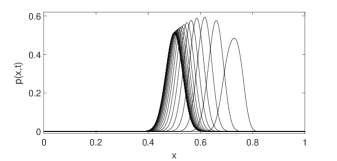
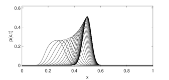
Figure 1: These two pictures illustrate the dominant behavior of convection for short times. (Left) convection moves solution toward the steady state from the right side to the left one for $R_{0}=2$ and $N=200$, (Right) convection moves solution toward the steady state from the left side to the right one for the same parameter values.

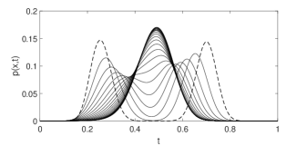
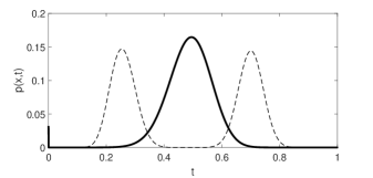
Figure 2: These two pictures illustrate short-time dynamics for $R_{0}=0$ and $N=100$ (on the left) and long time with blow up at the origin (on the right). The initial data are plotted with a dashed line.

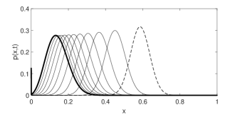
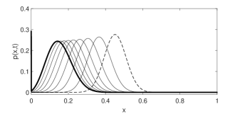
Figure 3: These two pictures illustrate the dominant behavior of convection for short times. (Left) convection moves solution toward the origin $R_{0}=0.5$ and $N=100$, where solution blows up. (Right) convection again moves solution toward the origin $R_{0}=1$ and $N=100$, where it blows up.

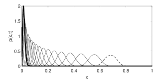
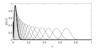
Figure 4: These two pictures illustrate the dominant behavior of convection for short times. (Left) convection moves solution toward the origin $R_{0}=0$ and $N=100$, where solution blows up. (Right) convection again moves solution toward the origin $R_{0}=0$ and $N=200$, where it blows up.

First, we will start with getting an analytical formula for a stationary solution for (1.1):

$$\frac{1}{2N}\frac{\partial}{\partial x}\bigl{(}\frac{\partial}{\partial x}(f(x)P_{s})-2Ng(x)P_{s}\bigr{)}=0\quad\text{in}\quad\Omega,$$ (3.1)

coupled with the boundary condition:

$$\frac{\partial}{\partial x}P_{s}(1)=-(2N-R_{0}+1)P_{s}(1).$$ (3.2)

Integrating (3.1) in $x$ and taking into account (3.2), we have

$$\frac{\partial}{\partial x}(f(x)P_{s})=2Ng(x)P_{s}.$$

It is apparent that this equation has a general solution

$$f(x)P_{s}(x)=\mathcal{C}\,F(x),$$ (3.3)

where we put

$$F(x):=e^{2N\int\limits_{0}^{x}{\tfrac{g(s)}{f(s)}ds}},\ \ \mathcal{C}:=\mathop{\lim}\limits_{x\to 0}f(x)p(x).$$

As a result, we obtain the explicit form of the classical stationary solution to (1.1)-(1.3)

$$P_{s}(x)=\tfrac{\mathcal{C}}{\omega(x)}\text{ where }\omega(x):=\tfrac{f(x)}{F(x)}.$$ (3.4)

Hence, the changing sign convection term for $R_{0}=2$ equals to zero at $x=0.5$ a wave-like solution moves toward this point forming a meta-stable steady state shape. The illustration that the solution short-time behavior is driven by the convection, as can be seen in Figures 1–2. It takes a long time for a meta-stable steady state to move mass toward the origin, this long-time dynamics is due to a slow diffusion effect and eventually the solution eventually blows-up at the origin. That, for two different sets of parameter values, as can be seen in Figures 3–4. All numerical simulations show high accuracy of mass conservation property even for long time computations that suggests an existence a delta function type weak solution which acts as a global attractor in this dynamical system.

3.2 Long-time behavior of a weak solution

Assuming that $\omega(x)$ is defined with (3.4) and

$$N\geqslant 1,\quad R_{0}\geqslant 0\quad\text{and}\quad 0\leqslant p_{0}(x)\in L_{\omega}^{2}(\Omega),$$

(see Section 2 as to the definition of $L_{\omega}^{2}(\Omega)$), we define a weak solution of (1.1)-(1.3) in the following sense.

Definition 3.1.

A non-negative function $p(x,t)\in L^{\infty}(0,T;L_{\omega}^{2}(\Omega))$ is a weak solution of problem (1.1)–(1.3) if

$$p_{t}\in L^{2}(0,T;H^{-1}(\Omega)),\ \ (\omega(x)p)_{x}\in L^{2}(Q_{T}),$$

and satisfies (1.1) in the sense

$$\int\limits_{0}^{T}{\Big{\langle}\frac{\partial p}{\partial t},\psi\Big{\rangle}_{H^{1},H^{-1}}\,dt}+\\ \iint\limits_{Q_{T}}{\bigl{(}\frac{1}{2N}\frac{\partial fp}{\partial x}-gp\bigr{)}\frac{\partial\psi}{\partial x}\,dxdt}=0$$

for all $\psi\in L^{2}(0,T;H_{0}^{1}(\Omega))$. Here $\langle u,v\rangle_{H^{1},H^{-1}}$ is a dual pair of elements $u\in H^{1}$ and $v\in H^{-1}$.

Now we are ready to state our first main result related to asymptotic behavior of a weak solution to (1.1)-(1.3).

Theorem 1.

(i) Let $0\leqslant p_{0}(x)\in L_{\omega}^{2}(\Omega)$ and $\mathop{\lim}\limits_{x\to 0}\omega(x)p(x,t)=0$ then a weak solution $p(x,t)$ satisfies the relation

$$\omega^{\frac{1}{2}}(x)p(x,t)\to 0\text{ strongly in }L^{2}(\Omega)\text{ as }t\to+\infty.$$

Moreover, if $(\omega(x)p_{0}(x))_{x}\in L^{2}(\Omega)$ then there is convergence

$$\omega(x)p(x,t)\to 0\text{ strongly in }W^{1,2}(\Omega)\text{ as }t\to+\infty.$$ (3.5)

(ii) Let $\omega^{\frac{1}{2}}(x)p_{0}(x)\in L_{\omega}^{2}(\Omega)$ and $\mathop{\lim}\limits_{x\to 0}\omega(x)p(x,t)=\mathcal{C}>0$ then for a weak solution $p(x,t)$ we have

$$\omega(x)p(x,t)\to\mathcal{C}\text{ strongly in }L^{2}(\Omega)\text{ as }t\to+\infty.$$ (3.6)

Moreover, if $\omega(x)(\omega(x)p_{0}(x))_{x}\in L^{2}(\Omega)$ then

$$\omega(x)\frac{\partial}{\partial x}(\omega(x)p(x,t))\to 0\text{ strongly in }L^{2}(\Omega)\text{ as }t\to+\infty.$$

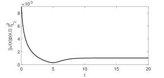
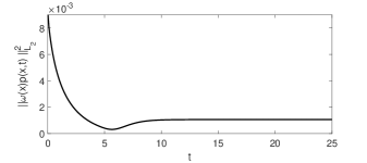
Figure 5: These two pictures illustrate convergence of weighted $L^{2}$ norm of $p(x,t)$ to a constant for $R_{0}=0$ and $N=100$ (on the left) and $R_{0}=0$ and $N=200$ (on the right).

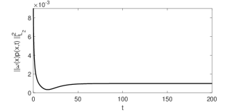
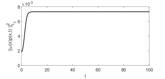
Figure 6: These two pictures illustrate convergence of weighted $L^{2}$ norm of $p(x,t)$ for $R_{0}=0.5$ and $N=100$ (on the left) and $R_{0}=2$ and $N=200$ (on the right).

Numerical simulations in Figures 5–6 illustrate the convergence result (3.6).

Remark 3.1.

Note that (3.5) implies

$$\int\limits_{\Omega}{p(x,t)\,dx}\to 0\text{ as }t\to+\infty,$$

whence we deduce that $p_{\infty}:=p(x,+\infty)=0$ for a. e. $x\in\bar{\Omega}$. On the other hand, (3.6) does the convergence to the steady state, i. e. $p_{\infty}=P_{s}$.

Proof of Theorem 1.

Introducing a new function $z:=\omega(x)p(x,t),$ we rewrite problem (1.1)–(1.3) in more suitable form:

$$\begin{cases}\omega^{-1}(x)\frac{\partial z}{\partial t}=\frac{1}{2N}\frac{\partial}{\partial x}\big{(}F(x)\frac{\partial z}{\partial x}\big{)},\qquad\quad(x,t)\in\Omega_{T},\\ \frac{\partial z}{\partial x}|_{x=1}=0\quad\text{ and }\quad z|_{x=0}=0,\qquad t\in[0,T],\\ z(x,0)=\omega(x)p_{0}(x):=z_{0}(x),\qquad\quad x\in\bar{\Omega}.\end{cases}$$ (3.7)

Note that if $z|_{x=0}=\mathcal{C}>0$ then for the new function $\tilde{z}=z-\mathcal{C}$ we again get problem similar to (3.7).

We begin to verify the point (i) of the theorem. To this end, multiplying the equation in (3.7) by $z(x,t)$ and integrating over $\Omega$, we obtain

$$\frac{1}{2}\frac{d}{dt}\int\limits_{\Omega}{\omega^{-1}(x)z^{2}\,dx}+\tfrac{1}{2N}\int\limits_{\Omega}{F(x)\bigg{(}\frac{\partial z}{\partial z}\bigg{)}^{2}\,dx}=\frac{1}{2N}F(x)z\frac{\partial z}{\partial z}\Bigl{|}_{0}^{1}=0.$$ (3.8)

Next, we take advantage of the Hardy inequality:

$$\int\limits_{\Omega}{\omega^{-1}(x)v^{2}\,dx}\leqslant C_{H}(R_{0})\int\limits_{\Omega}{F(x)\bigg{(}\frac{\partial v}{\partial x}\bigg{)}^{2}\,dx}$$

with $v(0)=0$. Here the constant $C_{H}(R_{0})$ satisfies the inequalities

$$A(R_{0})\leqslant C_{H}(R_{0})\leqslant 4A(R_{0})$$

with

$$A(R_{0})=\mathop{\sup}\limits_{r\in(0,1)}\Bigl{(}\int\limits_{0}^{r}{\tfrac{dx}{F(x)}}\Bigr{)}\Bigl{(}\int\limits_{r}^{1}{\tfrac{dx}{\omega(x)}}\Bigr{)}.$$

Thus, collecting (3.8) with the Hardy inequality, we end up with relations

$$\int\limits_{\Omega}{\omega^{-1}(x)z^{2}(x,t)\,dx}\leqslant e^{-\frac{t}{NC_{H}(R_{0})}}\int\limits_{\Omega}{\omega^{-1}(x)z_{0}^{2}(x)\,dx}\to 0\text{ as }t\to+\infty.$$ (3.9)

Multiplying the equation in (3.7) by $-\omega(x)\frac{\partial}{\partial x}\big{(}F(x)\frac{\partial z}{\partial x}\big{)}$ and integrating over $\Omega$, we obtain the equality

$$\frac{1}{2}\frac{d}{dt}\int\limits_{\Omega}{F(x)\bigg{(}\frac{\partial z}{\partial x}\bigg{)}^{2}\,dx}+\frac{1}{2N}\int\limits_{\Omega}{\omega(x)\bigg{(}\frac{\partial}{\partial x}\big{(}F(x)\frac{\partial z}{\partial x}\big{)}\bigg{)}^{2}\,dx}$$

$$=F(x)\frac{\partial z}{\partial t}\frac{\partial z}{\partial x}\Bigl{|}_{0}^{1},$$

which in turn provides

$$\frac{1}{2}\frac{d}{dt}\int\limits_{\Omega}{F(x)\bigg{(}\frac{\partial z}{\partial x}\bigg{)}^{2}\,dx}+\frac{1}{2N}\int\limits_{\Omega}{\omega(x)\bigg{(}\frac{\partial}{\partial x}\big{(}F(x)\frac{\partial z}{\partial x}\big{)}\bigg{)}^{2}\,dx}=0.$$ (3.10)

In order to handle the second term in the left-hand side of this equality, we will exploit the inequality

$$\int\limits_{\Omega}{\tfrac{v^{2}}{F(x)}\,dx}\leqslant C_{P}(R_{0})\int\limits_{\Omega}{\omega(x)\Big{(}\frac{\partial v}{\partial x}\Big{)}^{2}\,dx}\text{ with }v(1)=0,$$

where

$$C_{P}(R_{0})=\int\limits_{\Omega}{\tfrac{1}{F(x)}\Bigl{(}\int\limits_{x}^{1}{\tfrac{dy}{\omega(y)}}\Bigr{)}\,dx}.$$

Hence, we end up with relations

$$\int\limits_{\Omega}{F(x)\bigg{(}\frac{\partial z}{\partial x}\bigg{)}^{2}\,dx}\leqslant e^{-\frac{t}{NC_{P}(R_{0})}}\int\limits_{\Omega}{F(x)\bigg{(}\frac{\partial z_{0}}{\partial x}\bigg{)}^{2}\,dx}\to 0\text{ as }t\to+\infty.$$ (3.11)

As a result, we obtain the convergence

$$z(x,t)\to 0\quad\text{ strongly in }\quad W^{1,2}(\Omega)\text{ as }t\to+\infty.$$

if only the inequality holds

$$\int\limits_{\Omega}{\bigg{(}\omega^{-1}(x)z_{0}^{2}(x)+F(x)\bigg{(}\frac{\partial z_{0}}{\partial x}\bigg{)}^{2}\bigg{)}\,dx}<+\infty.$$

The simple consequence of this fact and convergence (3.11) is the bound

$$z(x,t)\leqslant x^{\frac{1}{2}}e^{-\frac{t}{2NC_{P}(R_{0})}}\Bigl{(}\int\limits_{\Omega}{F(x)\bigg{(}\frac{\partial z_{0}}{\partial x}\bigg{)}^{2}\,dx}\Bigr{)}^{\frac{1}{2}},$$

which in turn provides the desired relation

$$p(x,t)\leqslant\tfrac{x^{\frac{1}{2}}F(x)}{f(x)}e^{-\frac{t}{2NC_{P}(R_{0})}}\Bigl{(}\int\limits_{\Omega}{F(x)\bigg{(}\frac{\partial z_{0}}{\partial x}\bigg{)}^{2}\,dx}\Bigr{)}^{\frac{1}{2}}.$$

At this point we prove statement (ii) of the theorem. Multiplying (3.7) by $\omega(x)\psi(x)z(x,t)$ (as for the test function $\psi$ see Definition 3.1) and integrating over $\Omega$, we obtain

$$\frac{1}{2}\frac{d}{dt}\int\limits_{\Omega}{\psi(x)z^{2}\,dx}+\frac{1}{2N}\int\limits_{\Omega}{f(x)\psi(x)\bigg{(}\frac{\partial z}{\partial x}\bigg{)}^{2}\,dx}$$

$$=\frac{1}{2N}\bigg{(}f(x)\psi(x)z\frac{\partial z}{\partial x}-\frac{1}{2}(\omega(x)\psi(x))^{\prime}F(x)z^{2}\bigg{)}\bigg{|}_{0}^{1}$$

$$+\frac{1}{4N}\int\limits_{\Omega}z^{2}\frac{d}{dx}\bigg{(}F(x)\frac{d}{dx}\bigg{(}\omega(x)\psi(x)\bigg{)}\bigg{)}\,dx.$$

Then choosing here

$$\psi(x)=\omega^{-1}(x)\int\limits_{0}^{x}{\tfrac{dy}{F(y)}}=\tfrac{F(x)}{f(x)}\int\limits_{0}^{x}{\tfrac{dy}{F(y)}}\to\tfrac{1}{1+R_{0}}\text{ as }x\to 0,$$

we arrive at the equality

$$\frac{d}{dt}\int\limits_{\Omega}{\psi(x)z^{2}\,dx}+\frac{1}{N}\int\limits_{\Omega}{f(x)\psi(x)\bigg{(}\frac{\partial z}{\partial x}\bigg{)}^{2}\,dx}+\frac{1}{2N}z^{2}(1,t)=0.$$ (3.12)

In order to manage the left hand-side of this equality, we apply the Hardy inequality

$$\int\limits_{\Omega}{\psi(x)v^{2}\,dx}\leqslant C_{H}(R_{0})\int\limits_{\Omega}{f(x)\psi(x)v^{2}_{x}\,dx}\text{ with }v(0)=0,$$

where $A(R_{0})\leqslant C_{H}(R_{0})\leqslant 4A(R_{0})$ and

$$A(R_{0})=\mathop{\sup}\limits_{r\in(0,1)}\Bigl{(}\int\limits_{0}^{r}{\tfrac{dx}{f(x)\psi(x)}}\Bigr{)}\Bigl{(}\int\limits_{r}^{1}{\psi(x)\,dx}\Bigr{)}.$$

Thus, we easily conclude that

$$\int\limits_{\Omega}{\psi(x)z^{2}(x,t)\,dx}\leqslant e^{-\frac{t}{NC_{H}(R_{0})}}\int\limits_{\Omega}{\psi(x)z_{0}^{2}(x)\,dx}\to 0\text{ as }t\to+\infty.$$ (3.13)

Note that as $\psi(x)$ is bounded from bottom then we have $z\to 0$ in $L^{2}$ as $t\to+\infty$.

Now, multiplying the equation in (3.7) by $-\omega(x)\phi(x)\frac{\partial}{\partial x}\big{(}F(x)\frac{\partial z}{\partial x}\big{)}$ and integrating over $\Omega$, we obtain

$$\frac{1}{2}\frac{d}{dt}\int\limits_{\Omega}{\phi(x)F(x)\bigg{(}\frac{\partial z}{\partial x}\bigg{)}^{2}\,dx}+\frac{1}{2N}\int\limits_{\Omega}\omega(x)\phi(x)\bigg{(}\frac{\partial}{\partial x}\bigg{(}F(x)\frac{\partial z}{\partial x}\bigg{)}\bigg{)}^{2}\,dx$$

$$=\bigg{(}\phi(x)F(x)\frac{\partial z}{\partial t}\frac{\partial z}{\partial x}-\frac{1}{4N}\omega(x)\phi^{\prime}(x)F^{2}(x)\bigg{(}\frac{\partial z}{\partial x}\bigg{)}^{2}\bigg{)}\bigg{|}_{0}^{1}$$

$$+\frac{1}{4N}\int\limits_{\Omega}(\omega(x)\phi^{\prime}(x))^{\prime}F^{2}(x)\bigg{(}\frac{\partial z}{\partial x}\bigg{)}^{2}\,dx.$$

Taking $\phi(x)$ such that $(\omega(x)\phi^{\prime}(x))^{\prime}F^{2}(x)=2f(x)\psi(x)$, i. e.

$$\phi(x)=2\int\limits_{0}^{x}{\tfrac{1}{\omega(y)}\Bigl{(}\int\limits_{0}^{y}{\tfrac{1}{F(v)}\Bigl{(}\int\limits_{0}^{v}{\tfrac{ds}{F(s)}}\Bigr{)}dv}\Bigr{)}dy}\sim\tfrac{x^{2}}{2(R_{0}+1)}\text{ as }x\to 0,$$

we have

$$\frac{d}{dt}\int\limits_{\Omega}\phi(x)F(x)\bigg{(}\frac{\partial z}{\partial x}\bigg{)}^{2}\,dx+\frac{1}{N}\int\limits_{\Omega}\omega(x)\phi(x)\bigg{(}\frac{\partial}{\partial x}\bigg{(}F(x)\frac{\partial z}{\partial x}\bigg{)}\bigg{)}^{2}\,dx$$

$$=\frac{1}{N}\int\limits_{\Omega}f(x)\psi(x)\bigg{(}\frac{\partial z}{\partial x}\bigg{)}^{2}\,dx.$$

Collecting this equality with (3.12), we arrive at

$$\frac{d}{dt}\int\limits_{\Omega}\bigg{(}\phi(x)F(x)\bigg{(}\frac{\partial z}{\partial x}\bigg{)}^{2}+\psi(x)z^{2}\bigg{)}\,dx$$

$$+\frac{1}{N}\int\limits_{\Omega}\omega(x)\phi(x)\bigg{(}\frac{\partial}{\partial x}\bigg{(}F(x)\frac{\partial z}{\partial x}\bigg{)}\bigg{)}^{2}\,dx$$

$$+\frac{1}{2N}z^{2}(1,t)=0.$$ (3.14)

Then, applying the estimate

$$\int\limits_{\Omega}\frac{\phi(x)}{F(x)}v^{2}\,dx\leqslant C_{P}(R_{0})\int\limits_{\Omega}\omega(x)\phi(x)\bigg{(}\frac{\partial v}{\partial x}\bigg{)}^{2}\,dx\text{ with }v(1)=0,$$

where

$$C_{P}(R_{0})=\int\limits_{\Omega}{\tfrac{\phi(x)}{F(x)}\Bigl{(}\int\limits_{x}^{1}{\tfrac{dy}{\omega(y)\phi(y)}}\Bigr{)}\,dx},$$

to (3.2), we conclude

$$\int\limits_{\Omega}\phi(x)F(x)\bigg{(}\frac{\partial z}{\partial x}\bigg{)}^{2}\,dx\leqslant\Bigl{[}\int\limits_{\Omega}{\phi(x)F(x)\bigg{(}\frac{\partial z_{0}}{\partial x}\bigg{)}^{2}\,dx}$$

$$+\tfrac{1}{NC_{P}(R_{0})}\bigg{(}1-\tfrac{NC_{P}(R_{0})C_{H}(R_{0})}{C_{H}(R_{0})-C_{P}(R_{0})}+\tfrac{NC_{P}(R_{0})C_{H}(R_{0})}{C_{H}(R_{0})-C_{P}(R_{0})}e^{\tfrac{C_{H}(R_{0})-C_{P}(R_{0})}{NC_{P}(R_{0})C_{H}(R_{0})}t}\bigg{)}$$

$$\times\int\limits_{\Omega}\psi(x)z_{0}^{2}(x)\,dx\Bigr{]}e^{-\frac{t}{NC_{P}(R_{0})}}\to 0\quad\text{ as }\quad t\to+\infty.$$

As a result,

$$z(x,t)\to 0\text{ and }x\frac{\partial z}{\partial x}(x,t)\to 0\text{ strongly in }L^{2}(\Omega)\text{ as }t\to+\infty,$$

if only the inequality holds

$$\int\limits_{\Omega}{\bigg{(}\psi(x)z_{0}^{2}(x)+\phi(x)F(x)\bigg{(}\frac{\partial z_{0}}{\partial x}\bigg{)}^{2}\bigg{)}\,dx}<+\infty.$$

Finally, the passage to $p$ in these relations completes the proof of assertion (ii) and, as a consequence, of Theorem 1.

∎

4 Particular solutions

In this section, we will illustrate the result of Theorem 1 by particular solutions. First, we analyze classical solutions to problem (3.7) and then we discuss particular weak solutions.

4.1 Particular classical solutions

Introducing the new variable

$$s=\sqrt{2N}\int\limits_{0}^{x}{\tfrac{dy}{f^{\frac{1}{2}}(y)}},$$

and denoting

$$l(s):=\sqrt{2N}\tfrac{g(x)}{f^{\frac{1}{2}}(x)}=\sqrt{\tfrac{2N}{R_{0}}}\,\tfrac{\sin\bigl{(}\frac{1}{2}\sqrt{\frac{R_{0}}{2N}}s\bigr{)}\bigl{[}R_{0}-1-(R_{0}+1)\sin^{2}\bigl{(}\frac{1}{2}\sqrt{\frac{R_{0}}{2N}}s\bigr{)}\bigr{]}}{|\cos\bigl{(}\frac{1}{2}\sqrt{\frac{R_{0}}{2N}}s\bigr{)}|},$$

$$s_{1}:=2\sqrt{\tfrac{2N}{R_{0}}}\arcsin\bigl{(}\sqrt{\tfrac{R_{0}}{R_{0}+1}}\bigr{)},$$

we rewrite problem (3.7) in the form

$$\begin{cases}\frac{\partial z}{\partial t}=\frac{\partial^{2}z}{\partial s^{2}}+l(s)\frac{\partial z}{\partial s},\qquad s\in(0,s_{1}),\quad t\in(0,T),\\ z(0,t)=0,\quad\frac{\partial z}{\partial s}(s_{1},t)=0,\quad t\in[0,T].\end{cases}$$ (4.1)

It is worth noting that to reach (4.1), we incorporate the following simple verified relations:

$$s=\begin{cases}2\sqrt{\tfrac{2N}{R_{0}}}\arcsin\bigl{(}\sqrt{\tfrac{R_{0}}{R_{0}+1}}x^{\frac{1}{2}}\bigr{)},\quad\text{ if }\quad R_{0}>0,\\ \,\\ 2\sqrt{2N}x^{\frac{1}{2}},\qquad\quad\text{ if }\quad R_{0}=0,\end{cases}$$

or as consequence

$$x=\begin{cases}\tfrac{R_{0}+1}{R_{0}}\sin^{2}\bigl{(}\tfrac{1}{2}\sqrt{\tfrac{R_{0}}{2N}}s\bigr{)},\quad\text{ if }\quad R_{0}>0,\\ \,\\ \tfrac{1}{8N}s^{2},\qquad\qquad\text{ if }\quad R_{0}=0.\end{cases}$$

Separating variables in (4.1):

$$z(s,t)=T(t)S(s),$$

leads to the problems

$$\tfrac{T^{\prime}(t)}{T(t)}=\tfrac{S^{\prime\prime}(s)+l(s)S^{\prime}(s)}{S(s)}=-\lambda,$$

whence

$$T^{\prime}(t)=-\lambda T(t),$$

$$S^{\prime\prime}(s)+l(s)S^{\prime}(s)=-\lambda S(s)$$ (4.2)

with

$$S(0)=0,\ S^{\prime}(s_{1})=0.$$

After that, multiplying (4.2) by $p(s):=e^{\int\limits_{0}^{s}{l(y)\,dy}}$, we immediately obtain the equation

$$-(p(s)S^{\prime}(s))^{\prime}=\lambda p(s)S(s).$$

Then setting

$$U(s)=p^{\frac{1}{2}}(s)S(s)\quad q(s)=\tfrac{(p^{\frac{1}{2}}(s))^{\prime\prime}}{p^{\frac{1}{2}}(s)}=\tfrac{1}{2}\bigl{(}l^{\prime}(s)+\tfrac{1}{2}l^{2}(s)\bigr{)},$$

we arrive at the classical Sturm-Liouville problem with the continuous potential $q(s)$

$$\begin{cases}-U^{\prime\prime}(s)+q(s)U(s)=\lambda U(s),\qquad s\in(0,s_{1}),\\ U(0)=0,\quad U^{\prime}(s_{1})=0.\end{cases}$$ (4.3)

The standard technical calculations provide the following asymptotic behavior of eigenvalues and eigenfunctions to problem (4.3)

$$\lambda_{k}\sim(\tfrac{\pi}{s_{1}})^{2}\bigl{(}k+\tfrac{1}{2}\bigr{)}^{2},\ \ U_{k}(s)\sim\sin\bigl{(}\tfrac{\pi}{s_{1}}(k+\tfrac{1}{2})s\bigr{)},$$

or returning to (4.2)

$$\lambda_{k}\sim(\tfrac{\pi}{s_{1}})^{2}\bigl{(}k+\tfrac{1}{2}\bigr{)}^{2},\ \ S_{k}(s)\sim e^{-\frac{1}{2}\int\limits_{0}^{s}{l(y)\,dy}}\sin\bigl{(}\tfrac{\pi}{s_{1}}(k+\tfrac{1}{2})s\bigr{)}.$$

Thus, problem (4.1) has a particular solution

$$z(s,t)=\mathop{\sum}\limits_{k=0}^{+\infty}{c_{k}e^{-\lambda_{k}t}S_{k}(s)},$$

which in turn means

$$z(x,t)=\mathop{\sum}\limits_{k=0}^{+\infty}{c_{k}e^{-\lambda_{k}t}\varphi_{k}(x)},$$

where

$$\lambda_{k}\sim\tfrac{\pi^{2}}{N}\bigl{(}k+\tfrac{1}{2}\bigr{)}^{2},\ \ \varphi_{k}(x)\sim e^{-N^{\frac{3}{2}}x}\sin\Bigl{(}\pi(k+\tfrac{1}{2})\tfrac{\arcsin\bigl{(}\sqrt{\frac{R_{0}}{R_{0}+1}}x^{\frac{1}{2}}\bigr{)}}{\arcsin\bigl{(}\sqrt{\frac{R_{0}}{R_{0}+1}}\bigr{)}}\Bigr{)}.$$

Finally, keeping in mind the relation $z(x,t)=\omega(x)p(x,t)$, we deduce the particular classical solution

$$p(x,t)=\tfrac{1}{\omega(x)}\mathop{\sum}\limits_{k=0}^{+\infty}{c_{k}e^{-\lambda_{k}t}\varphi_{k}(x)}.$$

It is worth noting that the asymptotic behavior of the solution $\frac{C_{1}}{\sqrt{x}e^{C_{2}t}}$ as $x\to 0^{+}$ has a good agreement with Theorem 1 (i).

4.2 Particular weak solutions

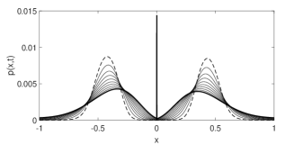
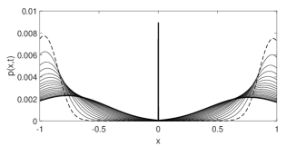
Figure 7: These two pictures illustrate existence of delta function type solution for a symmetrised problems with $R_{0}=0$ and $N=10$.

First of all we remark that with zero on the boundary the integral $\int_{0}^{a}f(z)\delta(z)dz$ is a priori not well defined. Then, we denote positive and non-negative cut of functions by $s1_{x>0}$ and $s1_{x\geq 0}$,respectively. It corresponds to integrating $\delta$ function against the function $f1_{x>0}$ (or possibly $f1_{x\geq 0}$ ) which is not continuous at the origin $x=0$, where the support of delta function lies. Some formal not analytically justified expressions have been used in a technical literature like $\int_{0}^{a}f(z)\delta(z)dz=\int_{-a}^{0}f(z)\delta(z)dz=\frac{1}{2}f(0)$. This is the reason why to justify a delta function type solution for our problem we will use a symmetrization method by considering a problem of extended domain $[-1,1]$. Now we look for a solution to a symmetrically extended problem (1.1)–(1.3) on the interval $(-1,1)$ in the form $p(x,t)=\eta(t)\delta_{0}(x)$.

Multiplying symmetrized equation (1.1) by $\phi(x)\in C^{2}[-1,1]$ with compact support and $\phi(0)\neq 0$, after integrating by parts in $Q_{T}:=(-1,1)\times(0,T)$, we have

$$\iint\limits_{Q_{T}}{\frac{\partial p}{\partial t}\phi(x)\,dxdt}=\frac{1}{2N}\iint\limits_{Q_{T}}{\bigl{(}\tilde{f}(x)p\phi^{\prime\prime}(x)+2N\tilde{g}(x)p\phi^{\prime}(x)\bigr{)}\,dxdt},$$

where $\tilde{f}$ and $\tilde{g}$ are even continuation of $f$ and $g$, accordingly. Taking $p(x,t)=\eta(t)\delta_{0}(x)$ in the last equality, we deduce that

$$(\eta(T)-\eta(0))\phi(0)=(\tfrac{1}{2N}f(0)\phi^{\prime\prime}(0)+g(0)\phi^{\prime}(0))\int\limits_{0}^{T}{\eta(t)\,dt}=0.$$

Thanks to the inequality $\phi(0)\neq 0$, we have

$$\eta(T)=\eta(0)=M>0.$$

As a result, symmetrized equation (1.1) has the following solution:

$$p(x,t)=M\delta_{0}(x)\text{ for all }(x,t)\in(-1,1)\times(0,+\infty).$$

Convergence of solution toward delta function is illustrated in Figure 7. It is interesting to mention that a non-smooth change of variables $y=2\,\sqrt{x}$ (for the case $R_{0}=0$) will remove the degeneracy from the equation but the whole long-time dynamics will not be recovered as a in terms of $y$ as a global attractor type solution $Ce^{t}$ that satisfied a no-flux boundary conditions in terms of variable $y$ will not be satisfying no-flux boundary conditions in terms of variable $x$. Although the $Ce^{t}$ solves the original problem with Neumann boundary conditions (which make the original problem ill-posed) it is unstable and a slight perturbation will drive the dynamics toward delta function.

5 Local classical solvability and asymptotic behavior of classical solutions near $x=0$

Here, we will discuss existence and behavior of a classical solution near the degenerate point $x=0$. Besides, we will analyze sufficient conditions on the given data in the model which provides the fulfillment of the conservation law. To this end, we consider the initial-boundary value problem to more general linear degenerate equation and the boundary condition than in the original problem (1.1)–(1.3).

Let $\Omega=(0,l)\subseteq\mathbb{R}_{+}=\{x:x>0\}$ be a segment with a boundary $\partial\Omega=\{x=0\}\cup\{x=l\}$. In our further consideration, we also use the notation $\Gamma_{1}$ for the right point of the boundary, i.e. $\Gamma_{1}=\{x=l\}$. For an arbitrary fixed time $T>0$, we denote

$$\partial\Omega_{T}=\partial\Omega\times[0,T]\quad\text{and}\quad\Gamma_{1,T}=\Gamma_{1}\times[0,T].$$

We analyze the linear degenerate equation in the unknown function $u=u(x,t):\Omega_{T}\to\mathbb{R},$

$$\frac{\partial u}{\partial t}-\mathcal{L}u=f(x,t)$$ (5.1)

supplemented with the initial condition

$$u(x,0)=u_{0}(x)\quad\text{in}\quad\bar{\Omega},$$ (5.2)

subject to the condition of the third kind (3BC):

$$\mathcal{M}u=\psi(x,t)\quad\text{on}\quad\Gamma_{1,T},$$ (5.3)

where the functions $f,u_{0}$ and $\psi$ are prescribed.

Coming to the operator involved, $\mathcal{L}$ is the linear degenerate elliptic operator of the second order with time-dependent coefficients, namely,

$$\mathcal{L}=xa_{0}(x,t)\frac{\partial^{2}}{\partial x^{2}}+a_{1}(x,t)\frac{\partial}{\partial x}+a_{2}(x,t),$$

while the operator $\mathcal{M}$ reads as

$$\mathcal{M}=b_{1}(x,t)\frac{\partial}{\partial x}+b_{2}(x,t).$$

5.1 Solvability of (5.1)-(5.3) in smooth classes and behavior of the solution at $x=0$

We start by introducing some general assumptions:

H1 (Conditions on the coefficients):

There exist positive $\delta_{0}$ and $\delta_{1}$ such that

$$a_{0}(x,t)\geq\delta_{0}\,\text{ for any }(x,t)\in\bar{\Omega}_{T},\,a_{1}(0,t)\geq\delta_{1}\text{ for any }t\in[0,T].$$ (5.4)

Besides,

$$a_{0},a_{1},a_{2}\in\mathcal{C}_{\alpha}^{\alpha,\alpha/2}(\bar{\Omega}_{T}),\,b_{1},b_{2}\in\mathcal{C}^{1+\alpha,\frac{1+\alpha}{2}}(\Gamma_{1,T}),$$

$$b_{1}(l,t)\neq 0\quad\text{for all }t\in[0,T].$$

H2 (Conditions on the given functions):

$$u_{0}(x)\in\mathcal{C}_{\alpha}^{2+\alpha}(\bar{\Omega}),\quad f\in\mathcal{C}_{\alpha}^{\alpha,\alpha/2}(\bar{\Omega}_{T}),\quad\psi\in\mathcal{C}^{1+\alpha,\frac{1+\alpha}{2}}(\Gamma_{1,T}).$$

H3 (Compatibility conditions):

When $x\in\Gamma_{1}$, the compatibility condition at $t=0$ holds

$$\mathcal{M}u_{0}(x)|_{t=0}=\psi(x,0).$$

Remark 5.1.

It is worth mentioning that assumption (5.4) on the coefficient $a_{1}$ and Fiker condition (see. i.e. [40, (1.13), p.17]) guarantee well-posedness in smooth classes of problem (5.1)-(5.3) (i.e. the initial-boundary value problem is stated without a boundary condition at the point $x=0$).

We are now in the position to state our main result concerning the solvability of (5.1)-(5.3).

Theorem 2.

Let $T>0$ be arbitrarily fixed and let assumptions H1-H3 hold. Then problem (5.1)-(5.3) admits a unique classical solution $u=u(x,t)$ on the space-time rectangle $\Omega_{T}$, satisfying regularity $u\in\mathcal{C}_{\alpha}^{2+\alpha,\frac{2+\alpha}{2}}(\bar{\Omega}_{T})$. Besides, the following estimate holds

$$\|u\|_{\mathcal{C}_{\alpha}^{2+\alpha,\frac{2+\alpha}{2}}(\bar{\Omega}_{T})} \leq C_{1}[\|u_{0}\|_{\mathcal{C}_{\alpha}^{2+\alpha}(\bar{\Omega})}+\|f\|_{\mathcal{C}_{\alpha}^{\alpha,\alpha/2}(\bar{\Omega}_{T})}+\|\psi\|_{\mathcal{C}^{1+\alpha,\frac{1+\alpha}{2}}}]$$

$$:=C_{1}\mathfrak{F}(u_{0},f,\psi)$$ (5.5)

with some $C_{1}>0$ being independent of the right-hand sides of (5.1)-(5.3).

If, in addition, the following assumption holds.

H4: There is a real $s_{0}$ such that

$$\begin{cases}s_{0}>\alpha,\\ \quad 2s_{0}a_{0}(0,t)+a_{1}(0,t)>0,\\ \underset{x\to 0}{\lim}\bigg{|}\frac{a_{1}(x,t)+(s_{0}-1)a_{0}(x,t)}{x}\bigg{|}<C,\end{cases}$$ (5.6)

for all $t\in[0,T]$ and

$$u_{0}\in E_{s_{0}}^{2+\alpha}(\bar{\Omega}),\quad f\in E_{s_{0}}^{\alpha,\alpha/2}(\bar{\Omega}_{T}).$$

Then, the classical solution $u$ satisfies the regularity

$$(x^{-s_{0}}u)\in\mathcal{C}_{\alpha}^{2+\alpha,\frac{2+\alpha}{2}}(\bar{\Omega}_{T}),$$

and

$$\|x^{-s_{0}}u\|_{\mathcal{C}_{\alpha}^{2+\alpha,\frac{2+\alpha}{2}}(\bar{\Omega}_{T})}\leq C_{2}[\|u_{0}\|_{E_{s_{0}}^{2+\alpha}(\bar{\Omega})}+\|f\|_{E_{s_{0}}^{\alpha,\alpha/2}(\bar{\Omega}_{T})}+\mathfrak{F}(u_{0},f,\psi)].$$ (5.7)

Remark 5.2.

It is apparent that estimate (5.7) where $s_{0}>\alpha$ provides the equality

$$u(0,t)=0\quad\text{for all}\quad t\in[0,T].$$ (5.8)

Example 5.1.

The following is an example of coefficients $a_{0},a_{1}$ and the weight $s_{0}$ satisfying condition (5.6) in the case of $\alpha\in(0,1/2)$:

$$s_{0}=\frac{1}{2}\quad\text{and}\quad a_{1}(x,t)=\frac{a_{0}(x,t)}{2},\quad(x,t)\in\bar{\Omega}_{T},$$

where $a_{0}$ meets requirement H1.

It is easy to verify that condition (5.6) is not satisfied in the case of original problem (1.1)–(1.3). That means, estimate (5.7) does not provid equality (5.8). Nevertheless, our next result states this equality under weaker assumptions on the coefficients than (5.6). Namely, we will assume additionally to H1-H3 the following conditions.

H5

Let $u_{0}\in E_{s}^{2+\alpha}(\bar{\Omega}),$ $f\in E_{s-1}^{\alpha,\alpha/2}(\bar{\Omega}_{T})$ with $s>1+\alpha$.

H6

Let $a_{0},a_{1}\in\mathcal{C}([0,T],\mathcal{C}^{1}(\bar{\Omega}))$. Besides, there is $\delta_{2}>0$ and the function $a(x,t)\in\mathcal{C}([0,T],\mathcal{C}^{1}(\bar{\Omega}))\cap\mathcal{C}_{\alpha/2}^{\alpha,\alpha/2}(\bar{\Omega}_{T})$ (including the case $a\equiv 0$) satisfying the inequality

$$\underset{\bar{\Omega}_{T}}{\sup}\frac{|a(x,t)|}{x}\leq C,$$

such that there holds

$$a_{1}(x,t)-a_{0}(x,t)=\delta_{2}+a(x,t).$$

Theorem 3.

Let $\psi\in\mathcal{C}^{1+\alpha,\frac{1+\alpha}{2}}(\Gamma_{1,T})$. Under assumptions H1, H3, H5 and H6, classical solution (5.1)-(5.3) vanishes at $x=0$ for all $t\in[0,T]$, i.e. equality (5.8) holds.

The rest part of this section is devoted to the proof of Theorems 2 and 3.

5.2 Some technical results

In this section we provide some technical results which are key points in the proof of Theorem 2 and as a consequence of Theorem 3.

5.2.1 Some auxiliary estimates

First we describe some properties of the solution to the initial-value problem for the degenerate linear equation, which will be key point in the proof of Theorem 2 in Section 5.3.

Let the function $v_{1}=v_{1}(x,t)$ solves the Cauchy problem

$$\begin{cases}\frac{\partial v_{1}}{\partial t}-x\frac{\partial^{2}v_{1}}{\partial x^{2}}-A_{1}\frac{\partial v_{1}}{\partial x}=F(x,t)\quad\text{in}\quad\mathbb{R}_{+,T}=\mathbb{R}_{+}\times(0,T),\\ v_{1}(x,0)=v_{1,0}(x),\quad\text{in}\quad\mathbb{R}_{+},\end{cases}$$ (5.9)

where $F$ and $v_{1,0}$ are some given functions, and $A_{1}$ is a given positive number.

The classical solvability of problem (5.9) was studied in [7, §2-3]. In particularly, the following result, stated as a lemma, subsumes Theorem 3.1 and estimate (2) in [7].

Lemma 5.1.

Let $A_{1}$ and $v_{1,0}\in\mathcal{C}_{\alpha}^{2+\alpha}(\bar{\mathbb{R}}_{+})$, $F\in\mathcal{C}_{\alpha}^{\alpha,\alpha/2}(\bar{\mathbb{R}}_{+,T})$. Besides, we assume that there exists a positive number $r_{0}$ such that

$$v_{1,0}(x)=F(x,t)=0\quad\text{if}\quad x>r_{0}.$$

Then, for any fixed $T>0$, there is a unique classical solution $v_{1}(x,t)$ to problem (5.9). In addition, the following estimate holds:

$$\|v_{1}\|_{\mathcal{C}_{\alpha}^{2+\alpha,\frac{2+\alpha}{2}}(\bar{\mathbb{R}}_{+,T})}\leq C[\|F\|_{\mathcal{C}_{\alpha}^{\alpha,\alpha/2}(\bar{\mathbb{R}}_{+,T})}+\|v_{1,0}\|_{\mathcal{C}_{\alpha}^{2+\alpha}(\bar{R}_{+})}].$$

Here, the generic constant $C$ is independent of the right-hand side in (5.9) and depends only on $A_{1}$ and $T$.

The next lemma allows us to reduce (5.1)-(5.3) to problem with homogenous initial data.

Lemma 5.2.

There exists a universal constant $C^{*}>0$ with the following property: for any functions $\mathcal{V}_{0}=\mathcal{V}_{0}(x)\in\mathcal{C}_{\alpha}^{2+\alpha}(\bar{\Omega})$ and $\mathcal{V}_{1}=\mathcal{V}_{1}(x)\in\mathcal{C}_{\alpha}^{\alpha}(\bar{\Omega})$, there exists a function $\mathcal{V}=\mathcal{V}(x,t)\in\mathcal{C}_{\alpha}^{2+\alpha,\frac{2+\alpha}{2}}(\bar{\Omega}_{T})$ such that

$$\mathcal{V}(x,0)=\mathcal{V}_{0}(x),\quad\frac{\partial\mathcal{V}}{\partial t}(x,0)=\mathcal{V}_{1}(x),$$

and

$$\|\mathcal{V}\|_{\mathcal{C}_{\alpha}^{2+\alpha,\frac{2+\alpha}{2}}(\bar{\Omega}_{T})}\leq C(\|\mathcal{V}_{0}\|_{\mathcal{C}_{\alpha}^{2+\alpha}(\bar{\Omega})}+\|\mathcal{V}_{1}\|_{\mathcal{C}_{\alpha}^{\alpha}(\bar{\Omega})}).$$

Proof.

Denoting

$$\mathcal{F}(x):=\mathcal{V}_{1}(x)-x\frac{\partial^{2}\mathcal{V}_{0}}{\partial x^{2}}(x)-A_{1}\frac{\partial\mathcal{V}_{0}}{\partial x},$$

we build (see [37, Theorem 4.1]) extensions $\bar{\mathcal{V}}_{0}$ and $\bar{\mathcal{F}}$ of the functions $\mathcal{V}_{0}$ and $\mathcal{F}$ on $\mathbb{R}_{+}$ such that

$$\|\bar{\mathcal{V}}_{0}\|_{\mathcal{C}_{\alpha}^{2+\alpha}(\bar{\mathbb{R}}_{+})} \leq C\|\mathcal{V}_{0}\|_{\mathcal{C}_{\alpha}^{2+\alpha}(\bar{\Omega})},$$ (5.10)

$$\|\bar{\mathcal{F}}\|_{\mathcal{C}_{\alpha}^{\alpha}(\bar{\mathbb{R}}_{+})} \leq C\|\mathcal{F}\|_{\mathcal{C}_{\alpha}^{\alpha}(\bar{\Omega})}\leq C(\|\mathcal{V}_{0}\|_{\mathcal{C}_{\alpha}^{2+\alpha}(\bar{\Omega})}+\|\mathcal{V}_{1}\|_{\mathcal{C}_{\alpha}^{\alpha}(\bar{\Omega})}),$$

and, besides, the functions $\bar{\mathcal{V}}_{0}$ and $\bar{\mathcal{F}}$ have compact supports. After that, we define the function $\mathcal{V}(x,t)$ to be the solution to the Cauchy problem

$$\begin{cases}\frac{\partial\mathcal{V}}{\partial t}-x\frac{\partial^{2}\mathcal{V}}{\partial x^{2}}-A_{1}\frac{\partial\mathcal{V}}{\partial x}=\bar{\mathcal{F}}(x)\quad\text{in }\mathbb{R}_{+,T},\\ \mathcal{V}(x,0)=\bar{\mathcal{V}}_{0}(x).\end{cases}$$

Applying Lemma 5.1 to this problem, and taking into account (5.10), the claim is proven. ∎

5.2.2 Domains. Some auxiliary propositions.

In order to prove the first part of Theorem 2, we will construct a regularizer (see [37, Section 4]). To this end, we need a special covering of the domain $\Omega$. We take two collections of open sets $\{\varpi^{m}\}$ and $\{\Omega^{m}\}$, which consist of a finite number $\varpi^{m}$ and $\Omega^{m}$ possessing the following properties for each small number $\lambda>0$ and any point $x^{m}\in\bar{\Omega}$:

1. Denoting by $\mathfrak{B}_{r}(x^{m})$ the ball about $x^{m}$ of radius $r$, we have that

   $$\varpi^{m}=\mathfrak{B}_{\lambda/2}(x^{m})\cap\bar{\Omega},\qquad\Omega^{m}=\mathfrak{B}_{\lambda}(x^{m})\cap\bar{\Omega},$$

   and

   $$\overline{\varpi^{m}}\subset\Omega^{m}\subset\bar{\Omega},\qquad\bigcup_{m}\varpi^{m}=\bigcup_{m}\Omega^{m}=\bar{\Omega}.$$

2. There exists a number $\mathcal{N}_{0}$ independent of $\lambda$ such that the intersection of any $\mathcal{N}_{0}+1$ distinct $\Omega^{m}$ (and consequently any $\mathcal{N}_{0}+1$ distinct $\varpi^{m}$) is empty.

The index $m$ belongs to one of three sets: $\mathfrak{M}$, $\mathfrak{N}_{0}$ or $\mathfrak{N}_{1}$, where

$$m\in\mathfrak{M}\quad \text{if }\overline{\Omega^{m}}\cap\partial\Omega=\emptyset,$$

$$m\in\mathfrak{N}_{0}\quad \text{if }\overline{\varpi^{m}}\cap\{x=0\}\neq\emptyset,$$

$$m\in\mathfrak{N}_{1}\quad \text{if }\overline{\varpi^{m}}\cap\Gamma_{1}\neq\emptyset.$$

Finally, denoting $\partial\Omega^{m}=\partial\Omega\cap\mathfrak{B}_{\lambda}(x^{m})$ and $\Gamma_{1}^{m}=\Gamma_{1}\cap\mathfrak{B}_{\lambda}(x^{m})$, we conclude that the covering $\{\varpi^{m}\}$ and $\{\Omega^{m}\}$ define a partition of unity for the domain $\Omega$. Let $\xi^{m}(x):$ $\Omega\to[0,1]$ be a smooth function such that

$$\xi^{m}(x)=1 \quad\text{if }x\in\overline{\varpi^{m}},$$

$$\xi^{m}(x)=0 \quad\text{if }x\in\bar{\Omega}\backslash\overline{\Omega^{m}},$$

$$\xi^{m}(x)\in(0,1) \quad\text{if }x\in\Omega^{m}\backslash\varpi^{m}.$$

Moreover,

$$|D_{x}^{j}\xi^{m}|\leq C\lambda^{-|j|},\qquad 1\leq|j|,\quad 1\leq\sum_{m}(\xi^{m})^{2}\leq\mathcal{N}_{0}.$$

Then, taking advantage of $\xi^{m}$, we define the function

$$\zeta^{m}:=\frac{\xi^{m}}{\sum_{j}(\xi^{j})^{2}}.$$ (5.11)

The properties of the functions $\xi^{m}$ tell us that the functions $\zeta^{m}$ vanish for $x\in\bar{\Omega}\backslash\overline{\Omega^{m}}$; and in addition, $|D_{x}^{j}\zeta^{m}|\leq C\lambda^{-|j|}$. Hence, the product $\zeta^{m}\xi^{m}$ defines the partition of unity via the formula

$$\sum_{m}\zeta^{m}\xi^{m}=1.$$

After that, in the spaces $\mathcal{C}_{\alpha,0}^{k+\alpha,\frac{k+\alpha}{2}\nu}(\bar{\Omega}_{T}),$ $k=0,1,2,$ we introduce the norms associated with the covering $\{\Omega^{m}\}$:

$$\langle\langle w\rangle\rangle_{\mathcal{C}_{\alpha}^{k+\alpha,\frac{k+\alpha}{2}}(\bar{\Omega}_{T})}:=\underset{m}{\sup}\|w\|_{\mathcal{C}_{\alpha}^{k+\alpha,\frac{k+\alpha}{2}}(\overline{\Omega^{m}}_{T})}.$$

Repeating the arguments of Chapter 4 in [37], we can assert the following.

Proposition 5.1.

Let $w\in\mathcal{C}_{\alpha,0}^{2+\alpha,\frac{2+\alpha}{2}}(\bar{\Omega}_{T})$. Then for $k=0,1,2,$

$$\|w\|_{\mathcal{C}([0,T],\mathcal{C}_{\alpha}^{k}(\bar{\Omega}))} \leq CT^{\frac{2+\alpha-k}{2}}\bigg{[}\langle\partial w/\partial t\rangle^{(\alpha/2)}_{t,0,\Omega_{T}}$$

$$+\bigg{\langle}x\frac{\partial w}{\partial x}\bigg{\rangle}_{t,0,\Omega_{T}}^{(\frac{\alpha}{2})}+\sum_{j=1}^{2}\bigg{\langle}x\frac{\partial^{j}w}{\partial x^{j}}\bigg{\rangle}_{t,0,\Omega_{T}}^{(\frac{2+\alpha-j}{2})}\bigg{]},$$

and, besides, for $k=0,1,$ there holds

$$\|w\|_{\mathcal{C}_{\alpha}^{k+\alpha,\frac{k+\alpha}{2}}(\bar{\Omega}_{T})}\leq CT^{\frac{2+\alpha-k}{2}}\bigg{[}\langle\partial w/\partial t\rangle^{(\alpha/2)}_{t,0,\Omega_{T}}+\sum_{j=1}^{2}\bigg{\langle}x\frac{\partial^{j}w}{\partial x^{j}}\bigg{\rangle}_{t,0,\Omega_{T}}^{(\frac{2+\alpha-j}{2})}\bigg{]},$$

$$\|\partial w/\partial t\|_{\mathcal{C}(\bar{\Omega}_{T})}\leq CT^{\frac{\alpha}{2}}\langle\partial w/\partial t\rangle^{(\alpha/2)}_{t,0,\Omega_{T}},$$

where the positive constant $C$ does not depend on $T$.

Next, for $\tau\in[0,T]$ and an arbitrarily given $0<\mathfrak{d}<1$, we set

$$\tau=\lambda^{2}\mathfrak{d}.$$ (5.12)

Proposition 5.2.

Let (5.12) hold. Then for $k=0,1,2,$ and any function $w\in\mathcal{C}_{\alpha,0}^{k+\alpha,\frac{k+\alpha}{2}}(\bar{\Omega}_{\tau})$, there is the following norm equivalence:

$$\langle\langle w\rangle\rangle_{\mathcal{C}_{\alpha}^{k+\alpha,\frac{k+\alpha}{2}}(\bar{\Omega}_{\tau})}\leq\|w\|_{\mathcal{C}_{\alpha}^{k+\alpha,\frac{k+\alpha}{2}}(\bar{\Omega}_{\tau})}\leq C\langle\langle w\rangle\rangle_{\mathcal{C}_{\alpha}^{k+\alpha,\frac{k+\alpha}{2}}(\bar{\Omega}_{\tau})},$$

where the positive constant $C$ is independent of $\lambda$ and $\tau$.

Proposition 5.3.

Let a function $\Phi_{m}(x)$ defined in $\Omega^{m}$ have the property

$$\bigg{|}\frac{\partial^{j}\Phi_{m}}{\partial x^{j}}(x)\bigg{|}\leq C\lambda^{-j},\quad 0\leq j\leq 2,$$

and the numbers $\tau$ and $\lambda$ are related via (5.12). Then for any function $w\in\mathcal{C}_{\alpha,0}^{k+\alpha,\frac{k+\alpha}{2}}(\bar{\Omega}_{\tau})$, $k=0,1,2$,

$$\|\Phi_{m}w\|_{\mathcal{C}_{\alpha}^{k+\alpha,\frac{k+\alpha}{2}}(\bar{\Omega}^{m}_{\tau})}\leq C\|w\|_{\mathcal{C}_{\alpha}^{k+\alpha,\frac{k+\alpha}{2}}(\bar{\Omega}^{m}_{\tau})},$$

where the positive constant $C$ does not depend on $\lambda$ and $\tau$.

Moreover, for $m\in\mathfrak{N}_{1}$ there holds

$$C\|\Phi_{m}w\|_{\mathcal{C}_{\alpha}^{k+\alpha,\frac{k+\alpha}{2}}(\bar{\Omega}^{m}_{\tau})}\leq\|w\|_{\mathcal{C}^{k+\alpha,\frac{k+\alpha}{2}}(\bar{\Omega}^{m}_{\tau})}\leq C\|\Phi_{m}w\|_{\mathcal{C}_{\alpha}^{k+\alpha,\frac{k+\alpha}{2}}(\bar{\Omega}^{m}_{\tau})},$$

and

$$C\|w\|_{\mathcal{C}_{\alpha}^{k+\alpha,\frac{k+\alpha}{2}}(\bar{\Omega}^{m}_{\tau})}\leq\|w\|_{\mathcal{C}^{k+\alpha,\frac{k+\alpha}{2}}(\bar{\Omega}^{m}_{\tau})}\leq C\|w\|_{\mathcal{C}_{\alpha}^{k+\alpha,\frac{k+\alpha}{2}}(\bar{\Omega}^{m}_{\tau})}.$$

Proposition 5.4.

Let (5.12) hold and

$$w(x,t)=\sum_{m\in\mathfrak{M}\,\cup\mathfrak{N}\,_{0}\cup\mathfrak{N}\,_{1}}w^{m}(x,t),$$

where $w^{m}\in\mathcal{C}_{\alpha,0}^{k+\alpha,\frac{k+\alpha}{2}}(\bar{\Omega}^{m}_{\tau})$ vanishes outside $\Omega^{m}$, $k=0,1,2$. Then

$$\langle\langle w\rangle\rangle_{\mathcal{C}_{\alpha}^{k+\alpha,\frac{k+\alpha}{2}}(\bar{\Omega}_{\tau})}\leq C\underset{m\in\mathfrak{M}\,\cup\mathfrak{N}\,_{0}\cup\mathfrak{N}\,_{1}}{\sup}\|w^{m}\|_{\mathcal{C}_{\alpha}^{k+\alpha,\frac{k+\alpha}{2}}(\bar{\Omega}^{m}_{\tau})}.$$

5.3 Proof of Theorem 2

It is worth noting that the second part Theorem 2 which concerns to estimate (5.7) is a simple consequence of (2) and (5.6). Indeed, in order to verify (5.7), it is enough to substitute the new unknown function $\mathcal{U}(x,t)=x^{-s_{0}}u(x,t)$ to (5.1)-(5.3) and then, taking into account assumptions H4, apply the first part of Theorem 2 and estimate (2). Thus, we are left to prove that (5.1)-(5.3) has a unique solution $u\in\mathcal{C}_{\alpha}^{2+\alpha,\frac{2+\alpha}{2}}(\bar{\Omega}_{T})$ satisfying (2). To this end, following arguments of §7-8 in Chapter 4 [37], we will construct an operator $\mathfrak{R}$ so-called a regularizer to (5.1)-(5.3) which allow us to construct the classical solution to this problem.

First of all, using Lemma 5.2 with $\mathcal{V}_{0}=u_{0}$ and $\mathcal{V}_{1}=\mathcal{L}u_{0}(x)|_{t=0}+f(x,0),$ $x\in\Omega$, we reduce (5.1)-(5.3) to the problem with homogenous initial data. Thus, we look for a solution to (5.1)-(5.3) in the form

$$u(x,t)=\mathcal{V}(x,t)+v(x,t)$$ (5.13)

where $\mathcal{V}(x,t)$ is built in Lemma 5.2. Coming to the new unknown function $v=v(x,t)$, it solves the following initial-boundary value problem

$$\begin{cases}\frac{\partial v}{\partial t}-\mathcal{L}v=\bar{f}\quad\text{in}\quad\Omega_{T},\\ v(x,0)=0\quad\text{in}\quad\bar{\Omega},\\ \mathcal{M}v=\bar{\psi}\quad\text{on}\quad\Gamma_{1,T},\end{cases}$$ (5.14)

where we put

$$\bar{f}=f(x,t)-\frac{\partial\mathcal{V}}{\partial t}+\mathcal{L}\mathcal{V},\quad\bar{\psi}=\psi(x,t)-\mathcal{V}|_{\Gamma_{1,T}}.$$

It is worth noting that assumptions H1-H3 and Lemma 5.2 provide the following smoothness

$$\bar{f}\in\mathcal{C}_{\alpha,0}^{\alpha,\alpha/2}(\bar{\Omega}_{T})\quad\text{and}\quad\bar{\psi}\in\mathcal{C}_{0}^{1+\alpha,\frac{1+\alpha}{2}}(\Gamma_{1,T}).$$ (5.15)

After that, for the sake of convenience, we rewrite problem (5.14) in more compact form

$$\mathcal{A}v=h\quad\text{with}\quad h=(\bar{f},\bar{\psi}),$$ (5.16)

where $\mathcal{A}$ is the linear operator defined by the left-hand side of (5.14). In other words, $\mathcal{A}v=\{\mathcal{A}_{0}v,\mathcal{A}_{1}v|_{\Gamma_{1,T}}\}$, where $\mathcal{A}_{0}$ is given by the left-hand side of the equation in (5.14) while $\mathcal{A}_{1}$ is defined by the left-hand side of 3BC in (5.14).

Setting now for $m\in\mathfrak{M}\cup\mathfrak{N}_{0}\cup\mathfrak{N}_{1}$,

$$a_{i}^{m}:=a_{i}(x^{m},0),\qquad\,\,b_{j}^{m}:=b_{j}(x^{m},0),$$

$$f_{m}:=\xi^{m}(x)\bar{f}(x,t),\quad\psi_{m}:=\xi^{m}(x)\bar{\psi}(x,t),$$

(where $\xi^{m},$ $\mathfrak{M}$, $\mathfrak{N}_{0}$, $\mathfrak{N}_{1}$ are defined in Subsection 5.2.2), we introduce the functions $V^{m}:=V^{m}(x,t)$, $m\in\mathfrak{M}\cup\mathfrak{N}_{0}\cup\mathfrak{N}_{1},$ as solutions to the following problems for $\tau\in(0,T]$ satisfying (5.12).

If $m\in\mathfrak{M}$, then

$$\begin{cases}\frac{\partial V^{m}}{\partial t}-x^{m}a_{0}^{m}\frac{\partial^{2}V^{m}}{\partial x^{2}}-a_{1}^{m}\frac{\partial V^{m}}{\partial x}=f_{m}\quad\text{in}\ \mathbb{R}_{\tau},\\ V^{m}(x,0)=0,\quad\text{in }\mathbb{R}.\end{cases}$$ (5.17)

Instead, if $m\in\mathfrak{N}_{1}$, then $V^{m}$ solves the initial-boundary value problem:

$$\begin{cases}\frac{\partial V^{m}}{\partial t}-x^{m}a_{0}^{m}\frac{\partial^{2}V^{m}}{\partial x^{2}}-a_{1}^{m}\frac{\partial V^{m}}{\partial x}=f_{m}\quad\text{in}\ \mathbb{R}_{+,\tau},\\ V^{m}(x,0)=0,\quad\text{in }\mathbb{R}_{+},\\ b_{1}^{m}\frac{\partial V^{m}}{\partial x}+b_{2}^{m}V^{m}=\psi^{m}\quad\text{in}\quad\partial\mathbb{R}_{+,\tau}.\end{cases}$$ (5.18)

Finally, in the case of $m\in\mathfrak{N}_{0}$, we define $V^{m}$ as a solution of the Cauchy problem:

$$\begin{cases}\frac{\partial V^{m}}{\partial t}-xa_{0}^{m}\frac{\partial^{2}V^{m}}{\partial x^{2}}-a_{1}^{m}\frac{\partial V^{m}}{\partial x}=f_{m}\quad\text{in}\ \mathbb{R}_{+,\tau},\\ V^{m}(x,0)=0\quad\text{in }\mathbb{R}_{+}.\end{cases}$$ (5.19)

It is easy to see that problems (5.17) and (5.18) are stated for usual (non-degenerate) parabolic linear equation, while problem (5.19) contains the degenerate parabolic equation similar to (5.1) with the coefficients satisfying to the Fiker condition.

Definition 5.1.

Let $\tau\in(0,T]$. An operator $\mathfrak{R}$ is called a regularizer, on the time-interval $[0,\tau]$, if

$$\mathfrak{R}:\mathcal{C}_{\alpha,0}^{\alpha,\frac{\alpha}{2}}(\bar{\Omega}_{\tau})\times\mathcal{C}_{0}^{1+\alpha,\frac{1+\alpha}{2}}(\Gamma_{1,\tau})\to\mathcal{C}_{\alpha,0}^{2+\alpha,\frac{2+\alpha}{2}}(\bar{\Omega}_{\tau}),$$

and

$$\mathfrak{R}h=\sum_{m\in\mathfrak{M}\cup\mathfrak{N}\,_{1}\cup\mathfrak{N}\,_{0}}\zeta^{m}(x)V^{m}(x,t),$$

where the functions $\zeta^{m}(x)$ and $V^{m}(x,t)$ are given in (5.11) and (5.17)-(5.19), respectively.

The operator $\mathfrak{R}$ enables us to build an inverse operator to $\mathcal{A}$. At this point, we state the key lemma.

Lemma 5.3.

Let $\tau\in(0,T]$ satisfy (5.12) and assume the hypotheses of Theorem 2. Then, setting

$$\mathcal{H}=\mathcal{C}_{\alpha,0}^{\alpha,\frac{\alpha}{2}}(\bar{\Omega}_{\tau})\times\mathcal{C}_{0}^{1+\alpha,\frac{1+\alpha}{2}}(\Gamma_{1,\tau}),$$

for any

$$h\in\mathcal{H}\qquad\text{and}\qquad v\in\mathcal{C}_{\alpha,0}^{2+\alpha,\frac{2+\alpha}{2}}(\bar{\Omega}_{\tau})$$

the following hold:

• $\mathfrak{R}$ is a bounded operator:

  $$\|\mathfrak{R}h\|_{\mathcal{C}_{\alpha}^{2+\alpha,\frac{2+\alpha}{2}}(\bar{\Omega}_{\tau})}\leq C\|h\|_{\mathcal{H}},$$

  where the positive constant $C$ is independent of $\lambda$ and $\tau$.

• There exist operators $\mathfrak{T}_{1}$ and $\mathfrak{T}_{2}$ such that

  $$\mathcal{A}\mathfrak{R}h=h+\mathfrak{T}_{1}h,\qquad\mathfrak{R}\mathcal{A}v=v+\mathfrak{T}_{2}v,$$ (5.20)

  where

  $$\|\mathfrak{T}_{1}h\|_{\mathcal{H}}\leq\frac{1}{2}\|h\|_{\mathcal{H}}\quad\text{and}\quad\|\mathfrak{T}_{2}v\|_{\mathcal{C}_{\alpha}^{2+\alpha,\frac{2+\alpha}{2}}(\bar{\Omega}_{\tau})}\leq\frac{1}{2}\|v\|_{\mathcal{C}_{\alpha}^{2+\alpha,\frac{2+\alpha}{2}}(\bar{\Omega}_{\tau})}.$$

Proof.

First, we verify statement (i) of this claim. Simple linear changes of variables allow us to conclude that the results of Lemma 5.1 above and Theorem 6.1 in [37] hold in the case of problems (5.17)-(5.19). Thus, collecting this results with Propositions 5.1-5.4, we arrive at the estimate

$$\|\mathfrak{R}h\|_{\mathcal{C}_{\alpha}^{2+\alpha,\frac{2+\alpha}{2}}(\bar{\Omega}_{\tau})}\leq C\underset{m\in\mathfrak{M}\,\bigcup\mathfrak{N\,}\,_{1}\bigcup\mathfrak{N\,}\,_{0}}{\sup}\|V^{m}\|_{\mathcal{C}_{\alpha}^{2+\alpha,\frac{2+\alpha}{2}}(\bar{\Omega}^{m}_{\tau})}$$

$$\leq C\Big{[}\underset{m\in\mathfrak{M}\,\bigcup\mathfrak{N\,}\,_{1}\bigcup\mathfrak{N\,}\,_{0}}{\sup}\|\xi^{m}\bar{f}\|_{\mathcal{C}_{\alpha}^{\alpha,\frac{\alpha}{2}}(\bar{\Omega}^{m}_{\tau})}+\underset{m\in\mathfrak{N\,}\,_{1}}{\sup}\|\xi^{m}\bar{\psi}\|_{\mathcal{C}^{1+\alpha,\frac{1+\alpha}{2}\nu}(\Gamma^{m}_{1,\tau})}\Big{]}$$

$$\leq C\|h\|_{\mathcal{H}},$$

with the constant $C$ satisfying the assumptions of the present lemma. Thus, we complete the proof of (i).

Let us verify (ii) of this claim. Here we restrict ourself verification of the first equality in (5.20). The second one in (5.20) is checked in the same manner with using analogous arguments from [37, Chapter 4, $\S$ 7]. Collecting definition of the operator $\mathcal{A}$ (see (5.16)) with the properties of $\zeta^{m}$ and $\xi^{m}$, we conclude that

$$\mathcal{A}\mathfrak{R}h=\{\mathcal{A}_{0}\mathfrak{R}h,\mathcal{A}_{1}\mathfrak{R}h\big{|}_{\Gamma_{1,\tau}}\},$$

where

$$\mathcal{A}_{0}\mathfrak{R}h=\bar{f}+\mathfrak{T}_{1}^{1}h,\quad\mathcal{A}_{1}\mathfrak{R}h=\bar{\psi}+\mathfrak{T}_{1}^{2}h,$$

and

$$\mathfrak{T}_{1}^{1}h =a_{2}(x,t)\mathfrak{R}h-\sum_{m}\bigg{[}2xa_{0}(x,t)\frac{\partial\zeta^{m}}{\partial x}\frac{\partial V^{m}}{\partial x}+xa_{0}(x,t)V^{m}\frac{\partial^{2}\zeta^{m}}{\partial x^{2}}\bigg{]}$$

$$-\sum_{m\in\mathfrak{M}\,\bigcup\mathfrak{N\,}\,_{1}}\zeta^{m}[xa_{0}(x,t)-x^{m}a_{0}(x^{m},0)]\frac{\partial^{2}V^{m}}{\partial x^{2}}$$

$$-\sum_{m\in\mathfrak{N\,}_{0}}\zeta^{m}x[a_{0}(x,t)-a_{0}(x^{m},0)]\frac{\partial^{2}V^{m}}{\partial x^{2}};$$

$$\mathfrak{T}_{1}^{2}h =b_{2}(x,t)\mathfrak{R}h|_{\Gamma_{1,\tau}}+\sum_{m\in\mathfrak{N\,}\,_{1}}b_{1}(x,t)\frac{\partial\zeta^{m}}{\partial x}V^{m}|_{\Gamma_{1,\tau}}$$

$$+\sum_{m\in\mathfrak{N\,}\,_{1}}\zeta^{m}[b_{1}(x,t)-b_{1}(x^{m},0)]\frac{\partial V^{m}}{\partial x}|_{\Gamma_{1,\tau}}.$$

After that, appealing to Propositions 5.1-5.4, Lemma 5.1 above and Theorem 6.1. from [37], and taking into account assumptions H2 with the following easily verified inequalities:

$$\bigg{\|}x\zeta^{m}\frac{\partial^{2}V^{m}}{\partial x^{2}}\bigg{\|}_{\mathcal{C}_{\alpha}^{\alpha,\frac{\alpha}{2}}(\bar{\Omega}^{m}_{\tau})}\leq C[1+\mathfrak{d}^{\alpha/2}]\bigg{\|}x\frac{\partial^{2}V^{m}}{\partial x^{2}}\bigg{\|}_{\mathcal{C}_{\alpha}^{\alpha,\frac{\alpha}{2}}(\bar{\Omega}^{m}_{\tau})}\,m\in\mathfrak{N}_{0},$$

$$\bigg{\|}\zeta^{m}\frac{\partial^{2}V^{m}}{\partial x^{2}}\bigg{\|}_{\mathcal{C}_{\alpha}^{\alpha,\frac{\alpha}{2}}(\bar{\Omega}^{m}_{\tau})}\leq C[1+\mathfrak{d}^{\alpha/2}]\bigg{\|}\frac{\partial^{2}V^{m}}{\partial x^{2}}\bigg{\|}_{\mathcal{C}_{\alpha}^{\alpha,\frac{\alpha}{2}}(\bar{\Omega}^{m}_{\tau})}\,m\in\mathfrak{M}\cup\mathfrak{N}_{1},$$

$$\bigg{\|}x\frac{\partial\zeta^{m}}{\partial x}\frac{\partial V^{m}}{\partial x}\bigg{\|}_{\mathcal{C}_{\alpha}^{\alpha,\frac{\alpha}{2}}(\bar{\Omega}^{m}_{\tau})} \leq C\bigg{[}(\mathfrak{d}^{\frac{1+\alpha}{2}}+\mathfrak{d}^{\frac{1}{2}})\bigg{\langle}x\frac{\partial V^{m}}{\partial x}\bigg{\rangle}_{t,0,\Omega^{m}_{\tau}}^{(\frac{1+\alpha}{2})}$$

$$+\mathfrak{d}^{\frac{\alpha}{2}}\bigg{\langle}x\frac{\partial^{2}V^{m}}{\partial x^{2}}\bigg{\rangle}_{t,0,\Omega^{m}_{\tau}}^{(\frac{\alpha}{2})}\bigg{]},$$

$$\bigg{\|}xV^{m}\frac{\partial^{2}\zeta^{m}}{\partial x^{2}}\bigg{\|}_{\mathcal{C}_{\alpha}^{\alpha,\frac{\alpha}{2}}(\bar{\Omega}^{m}_{\tau})} \leq C\bigg{[}(1+\lambda^{\alpha})\mathfrak{d}^{\frac{2+\alpha}{2}}\bigg{\langle}\frac{\partial V^{m}}{\partial t}\bigg{\rangle}_{t,0,\Omega^{m}_{\tau}}^{(\frac{\alpha}{2})}$$

$$+\mathfrak{d}^{\frac{1+\alpha}{2}}\bigg{\langle}x\frac{\partial V^{m}}{\partial x}\bigg{\rangle}_{t,0,\Omega^{m}_{\tau}}^{(\frac{1+\alpha}{2})}\bigg{]},$$

where the positive constant $C$ is independent of $\lambda$ and $\tau$, we end up with the estimates:

$$\|\mathfrak{T}_{1}^{1}h\|_{\mathcal{C}_{\alpha}^{\alpha,\alpha/2}(\bar{\Omega}_{\tau})}\leq\frac{1}{4}\|h\|_{\mathcal{H}},\quad\|\mathfrak{T}_{1}^{2}h\|_{\mathcal{C}^{1+\alpha,\frac{1+\alpha}{2}}(\Gamma_{1,\tau})}\leq\frac{1}{4}\|h\|_{\mathcal{H}}.$$

In virtue of $\mathfrak{T}_{1}h=\{\mathfrak{T}_{1}^{1}h,\mathfrak{T}_{1}^{2}h\}$, the last inequalities provide the first equality (5.20). This finishes the proof of point (ii) and, consequence, the proof of Lemma 5.3. ∎

Lemma 5.3 and, namely, relation (5.20) means that the operators $(I+\mathfrak{T}_{1})$ and $(I+\mathfrak{T}_{2})$ (here $I$ is the identity) are invertible for a suitable small time $\tau$, and $(I+\mathfrak{T}_{j})^{-1},$ $j=1,2,$ are bounded. Hence, this arrives at the equalities

$$\mathcal{A}\mathfrak{R}(I+\mathfrak{T}_{1})^{-1}h=h,\quad(I+\mathfrak{T}_{1})^{-1}\mathfrak{R}v=v,$$

which imply that $\mathcal{A}$ has bounded right and left inverse operators such that

$$\mathfrak{R}(I+\mathfrak{T}_{1})^{-1}=(I+\mathfrak{T}_{2})^{-1}\mathfrak{R}=\mathcal{A}^{-1}.$$

Accordingly, the unique solution of (5.14) is given by

$$v=\mathcal{A}^{-1}(\bar{f},\bar{\psi}),$$

or returning to the function $u$ (see (5.13)), we obtain a unique solution to the original problem (5.1)-(5.3) for $t\in[0,\tau]$:

$$u(x,t)=\mathcal{V}(x,t)+\mathcal{A}^{-1}(\bar{f},\bar{\psi}).$$

The estimate of the norm of $\mathcal{A}^{-1}$ follows from the corresponding estimates in Lemma 5.3. Finally, inequality (2) is a simple consequence of Lemmas 5.2 and 5.3, and relations (5.13), (5.15).

As a result, we have proved Theorem 2 for a small time interval $[0,\tau]$. In order to obtain this result in the general case, i.e., for $t\in[0,T]$, all we need is to extend the constructed solution on the interval $[i\tau,(i+1)\tau],$ $i=1,2,...$ while the entire $[0,T]$ is exhausted. To this end, we collect the technique from $\S 8$, Chapter 4 in [37] with the arguments above in the case of $t\in[0,\tau]$. This allows us to have the classical solution $u$ on $[0,T]$, which satisfies inequality (2). This completes the proof of Theorem 2. ∎

Remark 5.3.

Actually, with nonessential modifications in the arguments, the solvability of (5.1)-(5.3) in the weighted Hölder classes $E_{s}^{2+\alpha,\frac{2+\alpha}{2}}(\bar{\Omega}_{\tau})$, $s\in\mathbb{R}$, can be proved without requirement (5.6). Indeed, as it follows from the proof of Theorem 2, one should obtain the results similar to Lemma 5.1 in $E_{s}^{2+\alpha,\frac{2+\alpha}{2}}(\bar{\mathbb{R}}_{+,\tau})$. To this end, it is enough to modify arguments of Sections 2-4 in [8].

5.4 Proof of Theorem 3

Performing simple calculations, we deduce that

$$\|u_{0}\|_{\mathcal{C}_{\alpha}^{2+\alpha}(\bar{\Omega})}\leq C\|u_{0}\|_{E_{s}^{2+\alpha}(\bar{\Omega})}\quad\text{and}\quad\|f\|_{\mathcal{C}_{\alpha}^{\alpha,\alpha/2}(\bar{\Omega}_{T})}\leq C\|f\|_{E_{s}^{\alpha,\alpha/2}(\bar{\Omega}_{T})}.$$

Thus, these relations and assumptions H1,H3 provide the one-valued classical solvability of (5.1)-(5.3) in $\mathcal{C}_{\alpha}^{2+\alpha,\frac{2+\alpha}{2}}(\bar{\Omega}_{T})$. Taking into account this fact, we easily conclude that equality (5.8) follows immediately from the estimate

$$\int\limits_{0}^{y}u^{2}(x,t)dx+\int\limits_{0}^{t}u^{2}(0,s)ds\leq C_{0}yt\rho(y)\,\text{for all}\,t\in[0,T],\,y\in(0,l^{\star}],$$ (5.21)

with $l^{\star}=\min\{1/2,l\}$, and the bounded function $\rho(y)\in\mathcal{C}([0,l])$ satisfying the equality

$$\rho(y)=O(y^{2\gamma-1})$$ (5.22)

for some $\gamma\in(1/2,1)$ and for small $y$. The positive constant $C_{0}$ in (5.21) depends only on $T,l$ and the corresponding norms of the coefficients $a_{i}$, $i=0,1,2,$ and the functions $u_{0},$ $\psi$, $f$.

Therefore, here we are left to verify (5.21). To this end, we will exploit the following strategy consisting in two main steps. In this first one, we prove (5.21) for time $t\in[0,\tau]$ where

$$\tau=\varepsilon^{\star}y^{\gamma}$$ (5.23)

with some $\varepsilon^{\star}\in(0,\min\{1,T(l^{\star})^{-\gamma}\})$.

After that, we demonstrate how the obtained estimate can be extended to the whole time interval $[\tau,T]$.

Step 1: Choosing some arbitrarily $y\in(0,l^{\star}]$, we multiply equation (5.1) by the solution $u$ and integrate over $(0,y)$. Standard calculations (as integrating by parts in the terms related with $\frac{\partial^{2}u}{\partial x^{2}}$ and $\frac{\partial u}{\partial x}$) yield

$$\frac{1}{2}\frac{d}{dt}\int\limits_{0}^{y}u^{2}(x,t)dx+\int\limits_{0}^{y}xa_{0}(x,t)\big{(}\frac{\partial u}{\partial x}\big{)}^{2}dx+\frac{\delta_{2}}{2}u^{2}(0,t)$$ (5.24)

$$=\int\limits_{0}^{y}\bigg{[}a_{2}(x,t)+\frac{1}{2}\frac{\partial a_{0}}{\partial x}(x,t)-\frac{1}{2}\frac{\partial a_{1}}{\partial x}(x,t)\bigg{]}u^{2}(x,t)dx$$

$$+ya_{0}(y,t)u(y,t)\frac{\partial u}{\partial x}(y,t)+\frac{1}{2}[a_{1}(y,t)-a_{2}(y,t)]u^{2}(y,t)$$

$$-\int\limits_{0}^{y}x\frac{\partial a_{0}}{\partial x}(x,t)u(x,t)\frac{\partial u}{\partial x}(x,t)dx+\int\limits_{0}^{y}f(x,t)u(x,t)dx.$$

Here, we used the facts: conditions H6 and the smoothness of the solution $u\in\mathcal{C}_{\alpha}^{2+\alpha,\frac{2+\alpha}{2}}(\bar{\Omega}_{T})$, which provide the equalities:

$$\underset{x\to 0}{\lim}xa_{0}(x,t)u(x,t)\frac{\partial u}{\partial x}(x,t)=0,$$

$$\underset{x\to 0}{\lim}[a_{1}(x,t)-a_{0}(x,t)]u^{2}(x,t)=\delta_{2}u^{2}(0,t).$$

Making use of H1 for the second term in the left-hand side of (5.24), and treating the two last terms in the right-hand side via Cauchy inequality, we arrive at

$$\frac{1}{2}\frac{d}{dt}\int\limits_{0}^{y}u^{2}(x,t)dx+\delta_{0}\int\limits_{0}^{y}x\big{(}\frac{\partial u}{\partial x}\big{)}^{2}dx+\frac{\delta_{2}}{2}u^{2}(0,t)$$

$$=\bigg{[}\underset{\bar{\Omega}_{T}}{\sup}\Bigg{|}a_{2}(x,t)+\frac{1}{2}\frac{\partial a_{0}}{\partial x}(x,t)-\frac{1}{2}\frac{\partial a_{1}}{\partial x}(x,t)\bigg{|}+\frac{1}{2}$$

$$+\frac{y}{\varepsilon}\underset{\bar{\Omega}_{T}}{\sup}\Bigg{|}\frac{\partial a_{0}}{\partial x}(x,t)\bigg{|}\bigg{]}\int\limits_{0}^{y}u^{2}(x,t)dx+y\,\underset{\bar{\Omega}_{T}}{\sup}|a_{0}(y,t)||u(y,t)|\bigg{|}\frac{\partial u}{\partial x}(y,t)\bigg{|}$$

$$+\frac{1}{2}[\delta_{2}+|a(y,t)|]u^{2}(y,t)+\varepsilon\int\limits_{0}^{y}x\bigg{[}\frac{\partial u}{\partial x}(x,t)\bigg{]}^{2}dx+\int\limits_{0}^{y}f^{2}(x,t)dx,$$

or, choosing $\varepsilon=\frac{\delta_{0}}{2}$ and appealing to H1, H5, we have

$$\frac{d}{dt}\int\limits_{0}^{y}u^{2}(x,t)dx+\int\limits_{0}^{y}x\big{(}\frac{\partial u}{\partial x}\big{)}^{2}dx+u^{2}(0,t)$$ (5.25)

$$\leq C_{0}^{1}\Big{\{}y|u(y,t)|\bigg{|}\frac{\partial u}{\partial x}(y,t)\bigg{|}+[1+y]u^{2}(y,t)$$

$$+\|f\|^{2}_{E_{s-1}^{\alpha,\alpha/2}(\bar{\Omega}_{T})}y^{2s-1}+\int\limits_{0}^{y}u^{2}(x,t)dx\Big{\}},$$

where the positive constant $C_{0}^{1}$ is defined with only the norms of the coefficients $a_{i}$ and is independent of $y$ and $\tau$.

In order to evaluate the first two terms in the right-hand side in this inequality, we appeal to estimate (2) and end up with the relations

$$y|u(y,t)|\bigg{|}\frac{\partial u}{\partial x}(y,t)\bigg{|}\leq C_{1}y\mathfrak{F}(u_{0},f,\psi)\bigg{[}t\bigg{|}\frac{\partial u}{\partial t}(y,t)\bigg{|}+u_{0}(y)\bigg{]}$$

$$\leq C_{1}y[t+y^{s}]\mathfrak{F}_{s}^{2}(u_{0},f,\psi),$$

and

$$u^{2}(y,t)\leq C_{1}[t^{2}+y^{2s}]\mathfrak{F}^{2}_{s}(u_{0},f,\psi),$$

where we set

$$\mathfrak{F}_{s}^{2}(u_{0},f,\psi)=\bigg{[}\|u_{0}\|_{E_{s}^{2+\alpha}(\bar{\Omega})}+\|f\|_{E_{s-1}^{\alpha,\alpha/2}(\bar{\Omega}_{T})}+\|\psi\|_{\mathcal{C}^{1+\alpha,\frac{1+\alpha}{2}}(\Gamma_{1,T})}\bigg{]}.$$

Then, taking into account these estimates, and coming to (5.25), we finally obtain

$$\frac{d}{dt}\int\limits_{0}^{y}u^{2}(x,t)dx+\int\limits_{0}^{y}x\big{(}\frac{\partial u}{\partial x}\big{)}^{2}dx+u^{2}(0,t)$$

$$\leq C_{0}^{1}\max\{1,C_{1}\}\mathfrak{F}_{s}^{2}(u_{0},f,\psi)[y^{2s-1}+yt+y^{s+1}+(t^{2}+y^{2s})(1+y)]$$

$$+C_{0}^{1}\int\limits_{0}^{y}u^{2}(x,t)dx,$$

or, after integrating over $(0,t)$,

$$\int\limits_{0}^{y}u^{2}(x,t)dx+\int\limits_{0}^{t}dz\int\limits_{0}^{y}x\big{(}\frac{\partial u}{\partial x}\big{)}^{2}dx+\int\limits_{0}^{t}u^{2}(0,z)dz$$

$$\leq C_{0}^{1}\int\limits_{0}^{t}dz\int\limits_{0}^{y}u^{2}(x,z)dx+C_{0}^{1}\max\{1,C_{1}\}\mathfrak{F}_{s}^{2}(u_{0},f,\psi)$$

$$\times(t[y^{2s-1}+yt+y^{s+1}+(t^{2}+y^{2s})(1+y)]+y^{2s+1}).$$

After that, the Gronwall inequality and relation (5.23) entail

$$\int\limits_{0}^{y}u^{2}(x,t)dx+\int\limits_{0}^{t}dz\int\limits_{0}^{y}x\big{(}\frac{\partial u}{\partial x}\big{)}^{2}dx+\int\limits_{0}^{t}u^{2}(0,z)dz\leq C_{0}ty\rho_{0}(y),$$ (5.26)

where we set

$$C_{0} :=C_{0}^{1}\max\{1,C_{1}\}\mathfrak{F}_{s}^{2}(u_{0},f,\psi)e^{TC_{0}^{1}},$$ (5.27)

$$\rho_{0}(y) :=y^{2s-2}+y^{2s-1}+y^{2s}+y^{s}+2\varepsilon^{\star}y^{\gamma}+(\varepsilon^{\star})^{2}y^{2\gamma-1}.$$

Since $1/2<\gamma<1$, $s>1+\alpha$ and $y<1/2$, we easily conclude that $\rho_{0}(y)$ meets requirement (5.22), and estimate (5.26) leads to (5.21) if $t\in[0,\tau]$.

Moreover, inequality (5.26) and the mean value theorem provides key estimate which will be exploited in the second step of our arguments:

$$u^{2}(0,t^{\star})\leq C_{0}y\rho_{0}(y)$$ (5.28)

with some $t^{\star}\in(0,\tau)$. For simplicity consideration, we put $t^{\star}=\tau/2$.

Step 2: At this point we proceed the technique which allows us to extend estimate (5.21) to the interval $[\tau,T]$. First of all, we extend this estimate from $[0,\tau]$ to $[\tau,3\tau/2]$. To this end, we introduce a new variable $\bar{t}=t-\tau/2$, $\bar{t}\in[0,\tau],$ if $t\in[\tau/2,3\tau/2]$, and denote

$$\bar{a}_{i} :=a_{i}(x,\bar{t}+\tau/2),\,i=0,1,2,\quad\quad\bar{b}_{j}:=b_{j}(x,\bar{t}+\tau/2),\,j=1,2,$$

$$\bar{\mathcal{L}} :=x\bar{a}_{0}\frac{\partial^{2}}{\partial x^{2}}+\bar{a}_{1}\frac{\partial}{\partial x}+\bar{a}_{0},\qquad\bar{\mathcal{M}}:=\bar{b}_{1}\frac{\partial}{\partial x}+\bar{b}_{2},$$

$$u (x,\tau/2):=u_{\tau/2}(x),\qquad\qquad\bar{u}(x,\bar{t}):=u(x,\bar{t}+\tau/2),$$

$$\bar{f} (x,\bar{t}):=f(x,\bar{t}+\tau/2),\qquad\quad\bar{\psi}(x,\bar{t}):=\psi(x,\bar{t}+\tau/2).$$

It is apparent that the coefficients $\bar{a}_{i},$ $\bar{b}_{j}$ and the functions $\bar{f},\bar{\psi}$ and $u_{\tau/2}(x)=\bar{u}(x,0)$ meet the requirements of Theorem 2 and condition H6, and, besides, $\bar{f}$ and $\bar{\psi}$ satisfy H5. Thus, recasting the arguments leading to estimate (5.26) (with changing $u_{0}(x)$ by $u_{\tau/2}(x)$) in the case of the problem

$$\begin{cases}\frac{\partial\bar{u}}{\partial\bar{t}}-\bar{\mathcal{L}}\bar{u}=\bar{f}\quad\text{in}\quad\Omega_{\tau},\\ \mathcal{M}\bar{u}=\bar{\psi}\quad\text{on}\quad\Gamma_{1,\tau},\\ \bar{u}(x,0)=u_{\tau/2}(x)\quad\text{in}\quad\bar{\Omega},\end{cases}$$

we conclude

$$\int\limits_{0}^{y}\bar{u}^{2}(x,\bar{t})dx+\int\limits_{0}^{\bar{t}}dz\int\limits_{0}^{y}x\bigg{(}\frac{\partial\bar{u}}{\partial x}\bigg{)}^{2}dx+\int\limits_{0}^{\bar{t}}\bar{u}^{2}(0,z)dz\leq C_{0}\bar{t}y\bar{\rho}_{0}(y).$$ (5.29)

Here (in virtue of (5.28)) the function

$$\bar{\rho}_{0}(y)=y^{2s-2}+(1+(\varepsilon^{\star})^{2})y^{2\gamma-1}+(1+2\varepsilon^{\star})y^{\gamma}+2y^{2\gamma}$$

satisfies (5.22). Besides, due to $y<1/2$ and $1/2<\gamma<1<s$, there holds

$$\bar{\rho}_{0}(y)>\rho_{0}(y).$$

Finally, collecting estimate (5.26) with (5.29) (where we come back from $\bar{u}$ to $u$), we deduce inequality (5.21) for $t\in[0,3\tau/2]$, with $\rho(y):=\bar{\rho}_{0}(y),$ and $C_{0}$ defining in (5.27). Other words, we have extended estimate (5.21) from $[0,\tau]$ to $[\tau,3\tau/2]$. By the same token, we repeat the procedure to continue the obtain estimate on the other intervals until the entire $[0,T]$ is exhausted. Finally, keeping in mind that $y$ was arbitrarily point in $[0,l^{\star}],$ estimate (5.21) holds for all $y\in[0,l^{\star}]$ and $t\in[0,T]$. This completes the proof of Theorem 3.∎

5.5 Conservation Law

In this section we discuss the properties of the solution to problem (5.1)-(5.3) which follow from Theorems 2 and 3. Namely, we describe sufficient conditions on the given data in (5.1)-(5.3) which ensure the fulfillment of the conservation law to the solution $u\in\mathcal{C}_{\alpha}^{2+\alpha,\frac{2+\alpha}{2}}(\bar{\Omega}_{T})$:

$$\frac{d}{dt}\int\limits_{\Omega}u(x,t)dx=0\quad\text{for all}\quad t\in[0,T].$$ (5.30)

First, we state additional assumptions on the coefficients and the right-hand side of the model.

H7: Let $a_{0}\in\mathcal{C}_{\alpha}^{\alpha,\alpha/2}(\bar{\Omega}_{\tau})\cap\mathcal{C}([0,T],\mathcal{C}^{2}(\bar{\Omega})),$ and the following equalities hold:

$$x\frac{\partial^{2}a_{0}}{\partial x^{2}}-\frac{\partial a_{1}}{\partial x}+2\frac{\partial a_{0}}{\partial x}+a_{2}=0\quad\text{for each }(x,t)\in\bar{\Omega}_{T},$$

$$b_{1}(x,t)=xa_{0}(x,t),\,b_{2}(x,t)=-a_{0}(x,t)-x\frac{\partial a_{0}}{\partial x}(x,t)+a_{1}(x,t)\,\text{on}\,\Gamma_{1,T},$$

$$\psi(l,t)=-\int\limits_{0}^{l}f(x,t)dx,\quad t\in[0,T].$$

Theorem 4.

Let $T>0$ be fixed and assumptions of Theorem 3 and H7 hold. Then the classical solution $u\in\mathcal{C}_{\alpha}^{2+\alpha,\frac{2+\alpha}{2}}(\bar{\Omega}_{T})$ satisfies equality (5.30) for all $t\in[0,T]$.

Proof.

First, we recall that Theorem 3 ensures the existence of the classical solution $u\in\mathcal{C}_{\alpha}^{2+\alpha,\frac{2+\alpha}{2}}(\bar{\Omega}_{T})$ which vanishes at $x=0$ for all $t\in[0,T]$. Taking into account this fact, and integrating equation (5.1) over $\Omega$, we deduce

$$\frac{d}{dt}\int\limits_{0}^{l}u(x,t)dx =\int\limits_{0}^{l}\Big{[}\frac{\partial^{2}}{\partial x^{2}}(xa_{0})-\frac{\partial a_{1}}{\partial x}+a_{2}\Big{]}u(x,t)dx+\int\limits_{0}^{l}f(x,t)dx$$

$$+\underset{x\to l}{\lim}\bigg{[}xa_{0}\frac{\partial u}{\partial x}-u\frac{\partial}{\partial x}(xa_{0})+a_{1}u\bigg{]}.$$

Then, taking advantage of H7 to the terms in the right-hand side of this equality, we arrive at the desired relation (5.30). This completes the proof of this claim. ∎

Remark 5.4.

As it follows from the proof of Theorem 4, the last three equalities in H7 can be changed by the more general condition:

$$\int\limits_{0}^{l}f(x,t)dx+\underset{x\to l}{\lim}\bigg{[}xa_{0}\frac{\partial u}{\partial x}-u\frac{\partial}{\partial x}(xa_{0})+a_{1}u\bigg{]}=0.$$

5.6 A priori estimates in the Sobolev spaces

Here we obtain a priori estimates in $L^{2}$ norms of solution to problem (5.1)-(5.3). We start with state additional assumption on the coefficients of equation (5.1).

H8: We require that

$$a_{1}(0,t)-a_{0}(0,t)\geq 0\quad\text{and}\quad\frac{\partial a_{0}}{\partial x}(0,t)<0\quad\text{for all}\quad t\in[0,T].$$

Lemma 5.4.

Let $T>0$ be fixed, assumptions H1,H8 hold. Moreover, we assume that $a_{0}\in\mathcal{C}([0,T],\mathcal{C}^{2}(\bar{\Omega})),$ $a_{1}\in\mathcal{C}([0,T],\mathcal{C}^{1}(\bar{\Omega})),$ $b_{1}$ and $b_{2}$ meet requirements H7. If a solution $u$ of problem (5.1)-(5.2) with homogenous condition (5.3) satisfies the equality

$$\underset{x\to 0}{\lim}xa_{0}u\frac{\partial u}{\partial x}=0\quad\text{for each}\quad t\in[0,T],$$ (5.31)

then the following estimate is fulfilled

$$\|u\|_{\mathcal{C}([0,T],L^{2}(\Omega))}+\|x^{1/2}\partial u/\partial x\|_{L^{2}(\Omega_{T})}+\|u(0,\cdot)\|_{L^{2}(0,T)}$$

$$\leq C[\|u_{0}\|_{L^{2}(\Omega)}+\|f\|_{L^{2}(\Omega_{T})}]$$

with the positive constant $C$ depending only on $T,$ $\Omega$ and corresponding norms of the coefficients $a_{i}$.

Proof.

We multiply equation (5.1) by $u(x,t)$ and integrate over $\Omega=[0,l]$. Taking into account H1 and the smoothness of $a_{i},$ we have

$$\frac{1}{2}\frac{d}{dt}\int\limits_{0}^{l}u^{2}(x,t)dx+\delta_{0}\int\limits_{0}^{l}x\big{(}\frac{\partial u}{\partial x}\big{)}^{2}dx+L_{0}(u)$$

$$\leq-L_{l}(u)+\int_{0}^{l}f^{2}dx+\frac{1}{2}\int\limits_{0}^{l}\bigg{[}2-\frac{\partial a_{1}}{\partial x}+\frac{\partial^{2}(xa_{0})}{\partial x^{2}}\bigg{]}u^{2}dx,$$

where we put

$$L_{0}(u) =\underset{x\to 0}{\lim}\bigg{[}xa_{0}u\frac{\partial u}{\partial x}+\frac{1}{2}\bigg{(}a_{1}-a_{0}-x\frac{\partial a_{0}}{\partial x}\bigg{)}u^{2}\bigg{]},$$

$$L_{l}(u) =\underset{x\to l}{\lim}\bigg{[}-xa_{0}u\frac{\partial u}{\partial x}-\frac{1}{2}\bigg{(}a_{1}-a_{0}-x\frac{\partial a_{0}}{\partial x}\bigg{)}u^{2}\bigg{]}.$$

Assumptions on the coefficients $b_{1}$, $b_{2}$ and conditions H8 with (5.31) provide inequalities:

$$L_{0}(u)\geq 0\quad\text{and}\quad-L_{l}(u)<0.$$

Appealing to these relations and conditions on $a_{i}$, we end up with the estimate

$$\frac{d}{dt}\int\limits_{0}^{l}u^{2}(x,t)dx+\int\limits_{0}^{l}x\big{(}\frac{\partial u}{\partial x}\big{)}^{2}dx+L_{0}(u)\leq C\bigg{[}\int_{0}^{l}f^{2}dx+\int\limits_{0}^{l}u^{2}dx\bigg{]},$$

where the positive $C$ depends only on the norms of $a_{i}$, $i=0,1,2.$

Finally, Gronwall inequality arrives at the desired estimate. ∎

Remark 5.5.

It is apparent that the classical solution constructed in Theorem 2 satisfies assumption (5.31) of Lemma 5.1.

5.7 Conclusions of Theorems 2-4 and Lemma 5.4

Coming to original problem (1.1)–(1.3), we conclude that this problem can be rewritten in the form of (5.1)-(5.3) with the following coefficients and the right-hand sides:

$$u(x,t) =p(x,t),\quad f(x,t)=\psi(x,t)=0,\quad u_{0}(x)=p_{0}(x),$$

$$a_{0}(x,t) =\frac{R_{0}+1-R_{0}x}{2N},\,a_{1}(x,t)=\frac{R_{0}+1-R_{0}x}{N}-x(R_{0}-1-R_{0}x),$$

$$a_{2}(x,t) =-\frac{R_{0}}{N}-R_{0}+1+2R_{0}x,\quad b_{1}(x,t)=x\frac{R_{0}+1-R_{0}x}{2N},$$

$$b_{2}(x,t) =-a_{0}(x,t)-x\frac{\partial a_{0}}{\partial x}(x,t)+a_{1}(x,t).$$

These representations tell us that all assumptions of Theorems 2, 3 and 4, Lemma 5.4 hold, and we can assert the following.

Theorem 5.

Let $T>0$ be fixed and $p_{0}$ meet requirements of Theorem 2. Then original problem (1.1)–(1.3) has a unique classical solution $p\in\mathcal{C}_{\alpha}^{2+\alpha,\frac{2+\alpha}{2}}(\bar{\Omega}_{T})$ satisfying estimates:

$$\|p\|_{\mathcal{C}_{\alpha}^{2+\alpha,\frac{2+\alpha}{2}}(\bar{\Omega}_{T})}\leq C\|p_{0}\|_{\mathcal{C}_{\alpha}^{2+\alpha}(\bar{\Omega})},$$

$$\|p\|_{\mathcal{C}([0,T],L^{2}(\Omega))}+\|\sqrt{x}\partial p/\partial x\|_{L^{2}(\Omega_{T})}+\|p(0,\cdot)\|_{L^{2}(0,T)}\leq C\|p_{0}\|_{L^{2}(\Omega)}.$$

If, in addition, $p_{0}$ meets assumptions of Theorem 3, then the solution $p$ vanishes at $x=0$ for all $t\in[0,T]$ and the conservation law to this solution holds, i.e.

$$\frac{d}{dt}\int\limits_{\Omega}p(x,t)dx=0\quad\text{for all}\quad t\in[0,T].$$

References

• [1] L.J.S. Allen, Some discrete-time SI, SIR, and SIS epidemic models, Mathematical Biosciences, 124(1) (1994) 83–105.
• [2] L. J. S. Allen, A. M. Burgin, Comparison of deterministic and stochastic SIS and SIR models in discrete time. Mathematical Biosciences, 163(1) (2000) 1–33.
• [3] D.G. Aronson, P. Besala, Uniqueness of solutions of the Cauchy problem for parabolic equations, J. Math. Anal. Appl., 13 (1966) 516–526.
• [4] S. Athreya, M. Barlow, R. Bass, E. Perkins, Degenerate stochastic differential equations and super-markov chains, Probability Theory Related Fields, 128 (2002) 484–520.
• [5] R. Bass, E. Perkins. Degenerate stochastic differential equations with HΓΆlder continous coefficients and supermarkov chains, Trunsactions Amer. Math. Society, 355(1) (2002) 373–405.
• [6] B.V. Bazaliy, S.P. Degtyarev, On a boundary-value problem for a strongly degenerate second-order elliptic equation in an angular domain, Ukrain. Math. J., 59(7) (2007) 955–975.
• [7] B.V. Bazaliy, N.V. Krasnoschek, Regularity of solutions to multidimensional free boundary problems for the porous medium equation, Math. Trudy, 5(2) (2002) 38–91.
• [8] B.V. Bazaliy, N. Vasylyeva, On the solvability of the Hele-Shaw model problem in weighted HΓΆlder spaces in a plane angle, Ukrainian Math. J., 52(11) (2000) 1647–1660.
• [9] N. T. J. Bailey, The mathematical theory of infectious diseases and its applications, 2nd Edition. Hafner Press [Macmillan Publishing Co., Inc.] New York, 1975.
• [10] V. Barbu, A. Favini, S. Romanelli, Degenerate evolution equations and regularity of their associated semigroups, Funkcialaj Ekvacioj, 39 (1996) 421–448.
• [11] S. Cerrai, P. ClΓ©ment, Well-posedness of the martingale problem for some degenerate diffusion processes occurring in dynamics of populations, Bul. Sci. Math., 128 (2004) 355–389.
• [12] F.A.C.C. Chalub, M.O. Souza, The SIR epidemic model from a PDE point of view, Mathematical and Computer Modelling, 53(7-8) (2011) 1568–1574.
• [13] A.S. Cherny, On the uniqueness in law and the pathwise uniqueness for stochastic differential equations, Theory of Probability and its Applications, 46(3) (2001) 483–497.
• [14] F.A.C.C. Chalub, M.O. Souza, Discrete and continuous SIS epidemic models: A unifying approach, Ecological Complexity 18 (2014) 83–95.
• [15] F.A.C.C. Chalub, M.O. Souza, From discrete to continuous evolution models: A unifying approach to drift-diffusion and replicator dynamics, Theor. Popul. Biol., 76(4) (2009) 268–277.
• [16] F.A.C.C. Chalub, M.O. Souza, A non-standard evolution problem arising in population genetics, Commun. Math. Sci., 7(2) (2009) 489–502.
• [17] F.A.C.C. Chalub, M.O. Souza, The frequency-dependent Wright-Fisher model: diffusive and non-diffusive approximations., J. Math. Biol., 68 (2013) 1089–1133.
• [18] L. Chen, I. Weth-Wadman, Fundamental solution to 1D degenerate diffusion equation, with locally bounded coefficients, J. Math. Anal. and Appl., 510(2) (2022) 125979.
• [19] A.S. Cherny, H.-J. Engelbert, Singular stochastic differential equations, Springer, Lecture Notes in Mathematics Series, 1858, 2005.
• [20] D.A. Dawson, P. March, Resolvent estimates for Fleming-Viot operaors and uniqueness of solutions to related martingale problems, J. Func. Anal., 132 (1995) 417–474.
• [21] S.P. Degtyarev, Solvability of the first initial-boundary value problem to degenerate parabolic equations in the domains with a singular boundary, Ukr. Math. Bull., 5(1) (2008) 59–82.
• [22] O. Diekmann, H. Heesterbeek, T. Britton, Mathematical tools for understanding infectious disease dynamics, Princeton, NJ: Princeton University Press, 2013.
• [23] C. L. Epstein, R. Mazzeo, Degenerate Diffusion Operators Arising in Population Biology, v 185 in the series Annals of Mathematics Studies, Princeton University Press, 320 p., 2013.
• [24] C. L. Epstein, R. Mazzeo, The geometric micro-local analysis of generalized Kimura and Heston diffusions, Analysis Topology in Nonlinear Differential Equations Progress and Their Applications, 85 (2014) 241–266.
• [25] C. L. Epstein, R. Mazzeo, Harnack inequalities and heat-kernel estimates for degenerate diffusion operators arising in population biology, Applied Math. Research eXpress, 2016(2) (2016) 217–280.
• [26] C. L. Epstein, C.A. Pop, The Feynman-kac formula and Harnack inequality for degenerate diffusion, Annuals Probabil., 45 (5) (2017) 3336–3384.
• [27] C. L. Epstein, C.A. Pop, Transition probabilities for degenerate diffusion arising in population genetics, Probability Theory Related Fields, 173 (2019) 537–603.
• [28] S.N. Ethier, A class of degenerate diffusion processes occurring in population genetics, Commun. Pure Appl. Math., 29 (1976) 483–493.
• [29] W. J. Ewens, Mathematical population genetics, 2nd Edition. v. 27. Springer, New York, 2004.
• [30] Z. Feng, W. Huang, C. Castillo-Chavez, Global behavior of a multi- group sis epidemic model with age structure, J. Differential Equat., 218(2) (2005) 292–324.
• [31] G. Fichera, Sulle equazioni differenziali lineri ellittico-paraboliche del secondo ordine, Atti Accad. Naz. Lincei. Mem. Cl. Sei. Fiz. Mat. Nat. Sez. I, 5 (1956) 1–30.
• [32] P.M.N. Feehan, C.A. Pop, A Schauder approach to degenerate-parabolic partial differential equations with unbound coefficients, J. Differential Equat., 254 (2013) 4401–4445.
• [33] P.M.N. Feehan, C.A. Pop, On the martingale problem for degenerate-parabolic partial differential operators with unbounded coefficients and a mimicking theorem for Ito processes, Trans. Amer. Math. Soc., 367 (2015) 7565–7593.
• [34] P.M.N. Feehan, C.A. Pop, Boundary-degenerate elliptic operators and HΓΆlder continuity for solutions to variational equations and inequalities, Ann. Inst. H. PoincarΓ©-Anal. Nonlin., 34 (2017) 1075–1129.
• [35] J.A. Goldstein, C.Y. Cin, Degenerate parabolic problems and wentzel boundary condition, Semigroup Theory Applications, Lecture Notes in Pure Appl. Math. 116 (1989) 189–199.
• [36] K.S. Kumar, A class of degenerate stochastic differential equations with non-lipschitz coefficients, Proc. Indian. Acad. Sci., 123(3) (2013) 443–454.
• [37] O.A. Ladyzhenskaia, V.A. Solonnikov, N.N. Uraltseva, Linear and quasilinear parabolic equations, Academic Press, New York, 1968.
• [38] D.D. Monticelli, F. Punzo, Distance from submanifolds with boundary and applications to PoincarΓ© inequalities and to elliptic and parabolic problems, J. Differential Equat., 267 (2019) 4274–4292.
• [39] C. Nobili, F. Punzo, Uniqueness for degenerate parabolic equations in weighted $L^{1}$ spaces, J. Evol. Equa., 22(50) (2022).
• [40] O.A. Oleinik, E.V. Radkevic, Second-order equations with non-negative characteristic form, 1st Edition, Springer-Verlag US, Boston MA, 1973.
• [41] E. Perkins, Dawson-watanable super-processes and measure-valued diffusion, Lecture Notes in Mathematics, Spring-Velag, Berlin, 1781, 2001.
• [42] C.A. Pop, $C^{0}-$ estimates and smoothness of solutions to the parabolic equation defined by Kimura operators, J. Functional Anal., 272 (2017) 47–82.
• [43] C.A. Pop, Existence, uniqueness and the strong markov property of solutions to Kimura diffusion with singular drift, Trans. Amer. Math. Soc., 369 (2017) 5543–5579.
• [44] M.A. Pozio, F. Punzo, A. Tesei, Criteria for well-posedness of degenerate elliptic and parabolic problems, J. Math. Pures Appl., 90 (2008) 353–386.
• [45] M.A. Pozio, F. Punzo, A. Tesei, Uniqueness and nonuniqueness of solutions to parabolic problems with singular coefficients, DCDS-A, 30 (2011) 891–916.
• [46] M.A. Pozio, A. Tesei, On the uniqueness of bounded solutions to singular parabolic problems, DCDS-A, 13 (2005) 117–137.
• [47] F. Punzo, Uniqueness of solutions to degenerate parabolic and elliptic equations in weighted Lebesgue spaces, Math. Nachr., 286 (2013) 1043–1054.
• [48] F. Punzo, Integral conditions for uniqueness of solutions to degenerate parabolic equations, J. Diff. Equa., 267 (1) (2019) 6555–6573.
• [49] D. Stroock, S.R.S. Varadhan, On degenerate elliptic-parabolic opertors of second order and their associate diffusion, Commun. Pure Appl. Math., 25 (1972) 651–713.
• [50] A. Venni, Maximal regularity for a singular parabolic problem, Rend. Sem. Mat. Univ. Politec. Torino, 52(1) (1994) 87–101.