Comparing baseball players across eras via the novel Full House Model

Abstract

We motivate a new methodological framework for era-adjusting baseball statistics. Our methodology is a crystallization of the conceptual ideas put forward by Stephen Jay Gould. We name this methodology the Full House Model in his honor. The Full House Model works by balancing the achievements of Major League Baseball (MLB) players within a given season and the size of the MLB eligible population. We demonstrate the utility of our Full House Model in an application of comparing baseball players’ performance statistics across eras. Our results reveal a radical reranking of baseball’s greatest players that is consistent with what one would expect under a sensible uniform talent generation assumption. Most importantly, we find that the greatest African American and Latino players now sit atop the greatest all-time lists of historical baseball players while conventional wisdom ranks such players lower. Our conclusions largely refute a consensus of baseball greatness that is reinforced by nostalgic bias, recorded statistics, and statistical methodologies which we argue are not suited to the task of comparing players across eras.

1. Department of Statistics, University of Illinois Urbana-Champaign
2. Department of History, University of Illinois Urbana-Champaign
3. FuboTV Inc.

1 Introduction

The career accomplishments of Babe Ruth, Ty Cobb, Honus Wagner, Christy Mathewson, and Walter Johnson earned them election as the first class inducted into the National Baseball Hall of Fame in Cooperstown, New York, in 1939. They, and other stars from their era, still loom large when it comes to the history of and nostalgia about the sport that is a key part of numerous baseball-playing nations such as Cuba, the Dominican Republic, Japan, the U.S., and Venezuela, and was once heralded as the American national pastime. That they performed in Major League Baseball (MLB) during an era where a color line divided the professional game has not prevented their lot from remaining standard-bearers of hitting and pitching excellence, that by which all the sport’s greats are measured.

Statistics to measure player productivity in determining their rosters also provide a vital means to assess the greatness of players across different eras. Not all baseball statistics translate in the same way across generations, however [Eck, 2020a]. The long period that racial segregation reigned in U.S. professional baseball (the late 1880s to 1947) presents a peculiar challenge in making cross-era comparisons. Ruth, Cobb, and Wagner, among others, amassed their statistics starring in segregated MLB. Even more, they have benefitted from reliance on statistics they accumulated during this era without an adjustment for the time period and the expanded talent pool that intensified competition for Major League roster spots after integration. The sway these players continue to hold speaks to the power of nostalgia and the need for a reckoning with the game’s history. It also motivates our effort to develop a complex statistical model that can better assess the historical record.

Several academics have attempted to develop methods can correct for era biases [Berry, Reese, and Larkey, 1999, Petersen, Penner, and Stanley, 2011, Schell, 2013, 2016, Petersen and Penner, 2020], but they have fallen short in their objective and their results remain biased, as discussed in Eck [2020a] and Eck [2020b]. In short, these previous attempts do not incorporate the evolving talent pool in calculations, which is necessary for understanding the changing distributions of achievement over time. The result is that existing methodologies produce a disproportionate number of players who began their career before baseball was integrated players in rankings of baseball’s greatest of all time. This era of baseball did not include a crucial population of eligible players. Another important barrier to correctly computing baseball statistics is nostalgia. Many of these methodologies suffer from the additional shortcoming that they are only appropriate for very specific statistics, e.g., batting average and home runs, because they rely on strong distributional assumptions and do not have more general applicability.

The starting place for the answer to this problem of comparing players across eras can be found in the work of Stephen Jay Gould. Gould [1996] suggested that the entire distribution of achievement, or “full house of variation,” is relevant when considering the achievements of baseball players across eras. This idea was also recognized as the starting place for an answer by Schell [2013] and Schell [2016], but these authors placed their focus on the full house of variation within the population of baseball players already within MLB with the hope that the standard deviation alone captures changing talent pools. Berry et al. [1999] assumed that the changing talent pool is captured by seasonal random effects without broader consideration of a changing talent pool that was produced by the dismantling of MLB’s color line and furthered by the acquisition of athletes from the Caribbean, Latin America, and Asia. Berry et al. [1999] then go as far as to say that:

“American sports are experiencing increasing diversity in the regions from which they draw players. The globalization has been less pronounced in MLB, where players are drawn mainly from the United States and other countries in the Americas. Baseball has remained fairly stable within the United States, where it has been an important part of the culture for more than a century.”

This rationale completely ignores the racial segregation that has plagued U.S. professional baseball throughout its history. Worse yet, Petersen et al. [2011] and Petersen and Penner [2020] invented a spurious narrative which concludes that segregated baseball was much better with Babe Ruth’s 59 home runs in 1921 being worth 214 home runs (in 2009) and his 714 career home runs being worth 1215 home runs (nearly double that of second-place) in their era-neutral context. In short, these authors [Berry, Reese, and Larkey, 1999, Petersen, Penner, and Stanley, 2011, Schell, 2013, 2016, Petersen and Penner, 2020] are, at best, implicitly assuming that the composition, including racial and socio-economic profile, of MLB players, is the same across time — which the research of Mark Armour and Daniel Leavitt on the racial composition of MLB [Armour and Levitt, 2016] demonstrated is clearly not the case. This also ignores, at minimum, the effects of globalization, world wars, changing MLB salaries, and media exposure that have greatly impacted the composition of players in the MLB since its inception.

The starting point for the model that we develop is also Gould’s full house of variation concept, because it relies on the premise that the distribution of achievement can change based on exogenous factors. What this means is that over time the game of baseball evolves as does the composition of MLB players, a concept that aligns with basic intuition and the history of the game. Unlike others who have studied the question of how to compare players across eras, our model accounts for the mechanism of how potential eligible players feed into the MLB. We assume that MLB talent is evenly distributed across the MLB eligible population and that the most talented people in that population are those that reach the MLB at any given time. Though these are assumptions, they are more appropriate than not considering a large portion of the eligible population without basis or prioritizing certain time periods. With this connection between achievement and talent made, we can estimate latent individual talent – missed by other models – from the observed MLB statistics. Under this approach, a high talent score requires that an MLB player is both better than their peers and played during a time in which the MLB eligible population is large. In this way, the model constructs an even playing field that extends across eras. Additionally, we do not require strong distributional assumptions on observed baseball statistics, resulting in applicability to any baseball statistics that has been historically calculated. However, we do assume that the talent-generating process is known. Through simulation, we demonstrate that player rankings are fairly robust to the specification of the talent-generating process.

We have taken the following three principal steps to construct the MLB eligible population. First, we construct the list of countries comprising the MLB eligible population using Census counts and other domestic and international population data for baseball-age players. We include a country’s population of aged 20-29 year old males by year in the MLB eligible population when a person from that country reaches the MLB. Most countries that have produced two or more players will be added to the MLB eligible population. Second, we consult the United States Census, Statistics Canada, United Nations population tables, and the World Bank to tally the MLB eligible population over time and attempt to weigh each year by each country’s interest in baseball using polling sources [Fimrite, 1977, Baird, 2005, Schmidt and Berri, 2005, Burgos Jr, 2007, Jamail, 2008, Baseball-Reference, 2022]. Third, we adjust population sizes to account for the effects of wars, and the rates of integration in the two traditional leagues which comprise the MLB [Armour, 2007] among other adjustments.

Our results indicate an era-neutral ranking of baseball players that is more appropriate than previous techniques. The rankings that we obtain conform to what is statistically expected when talent is assumed to be evenly distributed over time. In broad strokes, our rankings show that African-American and Latino baseball players now sit atop the lists of baseball’s greatest, a significant finding for a sport with a well-recorded history of racial segregation. We also show that a wide variety of statistics, other era-adjustment approaches, and media sources include an over-representation of players who began their career before baseball was integrated into their ranking of the game’s greatest players.

This paper is organized in the following manner. In Section 2, we motivate the Full House Model using parametric and nonparametric probability distributions to estimate the era-adjusted components in the new system. Additionally, we provide some theoretical properties of our model. In Section 3, we compare our Full House Model career rankings in baseball with other commonplace career rankings and other era-adjustment approaches. In Section 4, we provide some assumptions and specifications when applying the Full House Model to baseball data, especially for the batting and pitching statistics. In Section 5, we validate our Full House Model based on the sensitivity analysis of the eligible population and latent talent distribution. In Section 6, we discuss the perceptions behind the other era-adjustment approaches and possible extensions in future work.

2 Model Setting

We now motivate the structure of the Full House Model. Let $N_{i}$ denote the size of the MLB eligible population in year $i$. We will suppose the every individual $k=1,\ldots,N_{i}$ has an underlying talent value $X_{i,1},\ldots,X_{i,N_{i}}\stackrel{{\scriptstyle\text{ iid }}}{{\sim}}F_{X}$. We denote $X_{i,(j)}$ as the $j$th ordered talents in year $i$. We define $g_{i}\left(\cdot,\cdot\right)$ as the MLB inclusion function, where $g_{i}\left(X_{i,j},\textbf{X}_{i,-j}\right)=1$ indicates that individual $j$ is an active MLB player in the $i$th year, and $g_{i}\left(X_{i,j},\textbf{X}_{i,-j}\right)=0$ indicates that individual $j$ is not an active MLB player in the $i$th year. Let $\textbf{X}_{i,-j}$ be the vector of all individual talents not including the component $j$. We will assume that the most talented individuals in year $i$ are active players in the MLB so that

$$g_{i}\left(X_{i,j},\mathbf{X}_{i,-j}\right)=1\left(X_{i,j}\geq X_{i,(N_{i}-n_{i}+1)}\right),$$ (1)

where $n_{i}$ is the number of active MLB players in year $i$ and $1(\cdot)$ is the indicator function.

We now suppose that in year $i$ an active MLB player $j$ has an observed statistics $Y_{i,j}$. For example, $Y_{i,j}$ can be batting average or home runs per at bat. We suppose that $Y_{i,1},\ldots,Y_{i,n_{i}}\overset{iid}{\sim}F_{Y_{i}}$ where $F_{Y_{i}}$ will be continuous. We denote $Y_{i,(j)}$ as the $j$th ordered statistic for players in the MLB during year $i$. The key to the Full House Model is connecting talent values $X$ with observed statistics $Y$. To do this we assume that we can form pairs $(Y_{i,(j)},X_{i,(N_{i}-n_{i}+j))})$, $j=1,\ldots,n_{i}$. As an example, the highest performer in the MLB in year $i$ as judged by values $Y_{i,j}$ will be assumed to have the highest talent score in year $i$.

The setup of the Full House Model is notably different from other era-adjustment approaches motivated by baseball. Previous approaches only focus on observable components $Y_{i,j}$, while our methodology connects underlying talent to the observed statistics. In this way, previous approaches ignore a key component of the evolution of recorded baseball statistics, and the result of this is artificial preferential treatment to players from an older, less-sophisticated era of baseball. As Gould [1996] said:

“What possible argument could convince us that a smaller and more restricted pool of indifferently trained men might supply better hitters than our modern massive industry with its maximal monetary rewards: I’ll bet on the larger pool, recruitment of men of all races, and better, more careful training any day.”

The working mechanics of the Full House Model connect to the above quote. The distribution of $Y_{i}$ shrinks as a better trained, stronger incentivized, and more racially diverse population of baseball players competes in the MLB. However, $N_{i}$ increases as these changing dynamics take hold. The selection inclusion mechanism $g$ (1) balances a shrinking distribution of achievement $Y_{i}$ with an increase in $N_{i}$, the net of which tends to favor Gould’s bet. In the next sections we detail how to obtain latent talent values from the pairs $(Y_{i,(j)},X_{i,(N_{i}-n_{i}+1)})$.

2.1 Parametric distributions for baseball statistics

We now demonstrate how the Full House Model works in a parametric setting. Consider the pair $(Y_{i,(j)},X_{i,(N_{i}-n_{i}+j)})$ and suppose that the distribution corresponding to $Y_{i,j}$ from the $i$th system is known to belong to a continuous parametric family indexed by unknown parameter $\theta_{i},$ and let $F_{Y_{i}}(\cdot\mid\theta_{i})$ be a parametric CDF with parameter $\theta_{i}\in\mathbb{R}^{p_{Y_{i}}}$. We can estimate $\theta_{i}$ with $\hat{\theta_{i}}$ and plug the estimator into the CDF $F_{Y}(\cdot\mid\hat{\theta_{i}})$.

In order to connect the $Y_{i,(j)}$ and $X_{i,(N_{i}-n_{i}+j)}$ and obtain an estimate of the underlying talents, we will make use of the following classical order statistics properties,

$$F_{Y_{i}}\left(Y_{i,(j)}\mid\theta_{i}\right) \sim U_{i,(j)}, F_{Y_{i}}\left(Y_{i,(j)}\mid\hat{\theta_{i}}\right)\approx U_{i,(j)},$$

$$F_{Y_{i,(j)}}\left(Y_{i,(j)}\mid\theta_{i}\right) \sim U_{i,j}, F_{Y_{i,(j)}}\left(Y_{i,(j)}\mid\hat{\theta_{i}}\right)\approx U_{i,j},$$

where $\approx$ means approximately distributed, $\sim$ means distributed as, $U_{i,j}\sim U(0,1)$, and $U_{i,(j)}\sim\operatorname{Beta}(j,n_{i}+1-j)$ and the quality of the approximation in the right hand side depends upon the estimator $\hat{\theta}_{i}$ and the sample size.

We now connect the order statistics to the underlying talent distribution that comes from a population with $N_{i}\geq n_{i}$ observations when $F_{X}$ is known. This connection is established with

$$F_{X_{i,(N_{i}-n_{i}+j)}}^{-1}\left(F_{U_{i,(j)}}\left(F_{Y_{i}}\left(Y_{i,(j)}\mid\theta_{i}\right)\right)\right)\sim F_{X_{i,(N_{i}-n_{i}+j)}}^{-1}\left(F_{U_{i,(j)}}\left(U_{i,(j)}\right)\right)=X_{i,(N_{i}-n_{i}+j)}.$$

We estimate the above with

$$F_{X_{i,(N_{i}-n_{i}+j)}}^{-1}\left(F_{U_{i,(j)}}\left(F_{Y_{i}}\left(Y_{i,(j)}\mid\hat{\theta}_{i}\right)\right)\right)\approx F_{X_{i,(N_{i}-n_{i}+j)}}^{-1}\left(F_{U_{i,(j)}}\left(U_{i,(j)}\right)\right)=X_{i,(N_{i}-n_{i}+j)}.$$ (2)

2.2 Nonparametric distribution for baseball statistics

2.2.1 Past methods and challenges of nonparametric approach

The empirical distribution function $\widehat{F}_{Y_{i}}$ is a widely used nonparametric approach in estimating the cumulative distribution function. However, $\widehat{F}_{Y_{i}}$ fails in our setting because $\widehat{F}_{Y_{i}}(Y_{i,(n_{i})})=1$ which when mapped to $X$ values through a similar approach to (2) yields $X_{i,(N_{i})}=\sup_{x}\{x:F_{X}(x)<1\}$. The implication here is that the highest achiever in year $i$ is estimated to have maximal possible talent, and this is nonsense. Therefore, we have an extrapolation problem. There are many alternatives to $\widehat{F}_{Y_{i}}$. For example, one could use piecewise linear function estimation [Leenaerts and Bokhoven, 1998, Kaczynski et al., 2012], kernel estimation [Silverman, 1986] and semi-parametric conjugated estimation [Scholz, 1995].

The methodology of Kaczynski et al. [2012] involved transforming the original data values so that the mean and variance of the piecewise-linear cumulative density function model matches the mean and variance of the sample values. It only partially solves the extrapolation problem apparent in our application and the authors do not show that the discrepancy between the estimator and the empirical CDF decreases as the sample size increases. The kernel estimation from Silverman [1986] can perform poorly when estimating heavy-tailed distribution and over-emphasize the bumps in the density for heavy-tailed data. Semi-parametric conjugated estimation is widely used in dealing with the tail behavior of the distribution. Scholz [1995] extended the scope of these nonparametric confidence bounds by introducing an adaptive type of QQ-plot, which performs a regression model on the sample extremes against corresponding transformed probability using an extreme value distribution. The model fits the sample extremes reasonably well and provides a reliable estimation for the extrapolation problem. Stein [2020] uses parametric families of the generalized Pareto distribution that have flexible behavior in both tails, which works well for estimating all quantiles when both tails of a distribution are heavy-tailed.

These methods fit within a more general Full House Modeling paradigm than what we motivate here. However, in the application to baseball data, the range of the distribution is naturally constrained, and outlying talents corresponding to outlying talent is lauded for its rarity. The above methods do not properly capture this behavior, and, when implemented, can lead to nonsensical results. The methods mentioned above model outlying performances with heavier tails, and this effectively lowers the underlying talent of such rarified performances when these techniques are implemented. In the next sections we motivate a new approach that handles the extrapolation problem and manner that reward rarified performances.

2.2.2 New interpolated and extrapolated approach

In the nonparametric setting, we motivate a variant of a natural interpolated empirical CDF as an estimator of the system components distribution $F_{Y_{i}}$ to solve the problems mentioned in the previous section. We consider surrogate sample points to construct an interpolated version of the empirical CDF $\widetilde{F}_{Y_{i}}$ and this type of interpolated CDF is a standard technique to replace the empirical CDF [Kaczynski et al., 2012].

We construct the interpolated CDF in the following manner: We first construct surrogate sample points $\widetilde{Y}_{i,(1)},\ldots,\widetilde{Y}_{i,(n_{i}+1)}$ as,

$$\widetilde{Y}_{i,(1)} =Y_{i,(1)}-Y^{*}_{i}$$

$$\widetilde{Y}_{i,(j)} =\left(Y_{i,(j)}+Y_{i,(j-1)}\right)/2,\quad j=2,\ldots,n$$

$$\widetilde{Y}_{i,(n_{i}+1)} =Y_{i,(n_{i})}+Y^{**}_{i},$$

where $Y^{*}_{i}$ is the value to construct the lower bound and $Y^{**}_{i}$ is the value to construct the upper bound. With this construction, we build $\widetilde{F}_{Y}$ as

$$\widetilde{F}_{Y}(t)=\sum_{j=1}^{n_{i}}\left(\frac{j-1}{n_{i}}+\frac{t-\widetilde{Y}_{i,(j)}}{n_{i}\left(\widetilde{Y}_{i,(j+1)}-\widetilde{Y}_{i,(j)}\right)}\right)1\left(\widetilde{Y}_{i,(j)}\leq t<\widetilde{Y}_{i,(j+1)}\right)+1\left(t\geq\widetilde{Y}_{i,(n_{i}+1)}\right)$$ (3)

The estimator $\widetilde{F}_{Y}$ is desirable for three reasons. First, we found (3) to be quick computationally. Second, we do not assume that the observed minimum and observed maximum constitute the actual boundaries of the support of $Y$. Third, $\widetilde{F}_{Y}\left(Y_{i,(1)}\right)$ and $\widetilde{F}_{Y}\left(Y_{i,(n_{i})}\right)$ provide reasonable estimates for the cumulative probability at $Y_{i,(1)}$ and $Y_{i,(n_{i})}$ by considering their respective value of $Y^{*}_{i}$ and $Y^{**}_{i}$. Here $Y^{**}_{i}$ is chosen to measure how far the highest achiever in year $i$ stood from their peers where small values of $Y^{**}_{i}-Y_{i,(n_{i})}$ have the interpretation that $Y_{i,(n_{i})}$ is an outlying performance and large values of $Y^{**}_{i}-Y_{i,(n_{i})}$ indicate the opposite. Construction of an upper bound $Y^{**}_{i}$ follows from Gould’s concept of a right-wall of achievement within the context of our baseball application, i.e. there is only so much a body can physiologically do and performance, therefore, has an upper bound [Gould, 1996]. More details on the computation of $Y^{*}_{i}$ and $Y^{**}_{i}$ are in Section 2.2.3.

The approximations to facilitate our methodology are similar to the ones in the parametric case. The hidden trait values can be found using the

$$F_{X_{i,(N_{i}-n_{i}+j)}}^{-1}\left(F_{U_{i,(j)}}\left(F_{Y_{i}}\left(y_{i,(j)}\right)\right)\right)\sim F_{X_{i,(N_{i}-n_{i}+j)}}^{-1}\left(F_{U_{i,(j)}}\left(U_{i,(j)}\right)\right)=X_{i,(N_{i}-n_{i}+j)},$$

and the above can be estimated with

$$F_{X_{i,(N_{i}-n_{i}+j)}}^{-1}\left(F_{U_{i,(j)}}\left(\widetilde{F}_{Y_{i}}\left(y_{i,(j)}\right)\right)\right)\approx F_{X_{i,(N_{i}-n_{i}+j)}}^{-1}\left(F_{U_{i,(j)}}\left(U_{i,(j)}\right)\right)=X_{i,(N_{i}-n_{i}+j)}.$$ (4)

Notice that $\widetilde{F}_{Y_{i}}(t)$ is explicitly constructed to be close to $\widehat{F}_{Y_{i}}(t)$. We formalize this statement below.

Proposition 2.1.

Let $\widetilde{F}_{Y_{i}}(t)$ be defined as in (2) and let $\widehat{F}_{Y_{i}}(t)$ be the empirical distribution function. Then,

$$\sup_{t\in\mathbb{R}}\left|\tilde{F}_{Y_{i}}(t)-\widehat{F}_{Y_{i}}(t)\right|\leq\frac{1}{n}$$

This leads to a Glivenko-Cantelli result which is appropriate for $\widetilde{F}_{Y}$.

Corollary 2.1.1.

Let $\widetilde{F}_{Y_{i}}(t)$ be defined as in (1) and let $\widehat{F}_{Y_{i}}(t)$ be the empirical distribution function. Then,

$$\sup_{t\in\mathbb{R}}\left|\widetilde{F}_{Y_{i}}(t)-F_{Y_{i}}(t)\right|\stackrel{{\scriptstyle a.s}}{{\longrightarrow}}0$$

Proofs of these results are included in the Appendix 7.2. Corollary 2.1.1 shows that the interpolated empirical distribution function is a serviceable estimator for $F_{Y_{i}}$.

2.2.3 Choosing $Y^{*}_{i}$ and $Y^{**}_{i}$

The cumulative probabilities $\widetilde{F}_{Y}\left(Y_{i,(1)}\right)$ and $\widetilde{F}_{Y}\left(Y_{i,(n_{i})}\right)$ are, respectively, functions $Y^{*}_{i}$ and $Y^{**}_{i}$. In this section we describe the role of $Y^{*}_{i}$ and $Y^{**}_{i}$ and how these quantities are chosen in our application to historical baseball rankings.

The lower bound $Y^{*}_{i}$ determines the lower tail behavior of talent distribution, and in fact, most normal or low talents would concentrate in a similar scale or size [Newman, 2005]. Therefore $Y^{*}_{i}$ can be a small positive value, we define $Y^{*}_{i}=Y_{i,(2)}-Y_{i,(1)}$. This is not the only choice of $Y^{*}_{i}$, and other reasonable choices can also be set to the $Y^{*}_{i}$.

We now discuss how we calculate $Y^{**}_{i}$. Our approach follows a simple nonparametric tail extrapolation method motivated in Scholz [1995]. This method involves linear extrapolation on the different types of transformed percentiles, such as linear transformation, logit transformation, and logit transformation with quadratic terms. We now describe this approach.

First, some preliminaries. The $p$-quantile $y_{p}$ of $F$ is defined as the smallest value for which $F\left(y_{p}\right)=p$, i.e. $y_{p}=\inf\{y:F(y)\geq p\}$. Hence $P\left(Y_{i,j}\leq y_{p}\right)=p$. Now suppose that $p_{i,j,\gamma,n_{i}}$ is the value of $p$ that satisfies $\gamma=P\left(Y_{i,(j)}\geq y_{p}\right)$. For each $j$ and $\gamma$ there is an approximation of $p_{i,j,\gamma,n_{i}}$ for choices of $\gamma$ [Scholz, 1995]. Hoaglin et al. [1983] gave a specific justified approximation of $p_{i,j,\gamma,n_{i}}$ when $\gamma=0.5$. This approximation is,

$$p_{i,j,.5,n_{i}}\approx\frac{j-\frac{1}{3}}{n_{i}+\frac{1}{3}}.$$

With this approximation, we have a tractable means to connect the order statistics $Y_{i,(j)}$ to percentile values $p_{i,j,.5,n_{i}}$ corresponding to the median value of a quantile $y_{p_{i,j,.5,n_{i}}}$.

Following Scholz [1995], we consider the regression fit on points $(h(p_{i,j,.5,n_{i}}),Y_{i,(j)})$, $j=n_{i}-k+1,\ldots,n_{i}$, where $k$ is the number of extreme data values to use in the extrapolation step, and $h$ is a function of the percentiles. The specific choices that we considered for $h$ are similar to those in Scholz [1995]:

• linear transformation: $h_{\theta}(p)=\theta_{1}+\theta_{2}p$;

• logit transformation: $h_{\theta}(p)=\theta_{1}+\theta_{2}\log(p/(1-p))$;

• logit transformation with the quadratic term: $h_{\theta}(p)=\theta_{1}+\theta_{2}\log(p/(1-p))+\theta_{3}\left[\log(p/(1-p))\right]^{2}$.

In practice, we chose $h$ among the candidates by selecting whichever $h$ maximized regression fit as judged by adjusted $R^{2}$ values. Selection of $k$ can be found in the Appendix 7.1 and the Supplementary Materials. The method for determining $k$ follows from Scholz [1995], Castillo [2012], and Dekkers et al. [1989].

With this setup, we compute $Y_{i}^{**}$ through a connection between $\widetilde{F}_{Y_{i}}(Y_{i,(n_{i})})$ and the regression fit on points $(h(p_{i,j,.5,n_{i}}),Y_{i,(j)})$, $j=n_{i}-k+1,\ldots,n_{i}$. Specifically, we find $Y_{i}^{**}$ as the solution of the following optimization problem

$$Y_{i}^{**}=\text{argmin}_{y}\Big{|}h^{-1}(Y_{i,(n_{i})})-\widetilde{F}_{Y_{i}}(Y_{i,(n_{i})};y)\Big{|},$$ (5)

where $\widetilde{F}_{Y_{i}}(\cdot;y)$ is $\widetilde{F}_{Y_{i}}$ defined with respect to a value $y$ replacing $Y_{i}^{**}$ in its construction. The intuition of (5) for large outlying values of $Y_{i,(n_{i})}$ is as follows: the value of $h^{-1}(Y_{i,(n_{i})})$ corresponds to percentile $p_{i,n_{i},.5,n_{i}}$ that is close to $1$, and this pulls $Y_{i}^{**}$ towards zero so that $\widetilde{F}_{Y_{i}}(Y_{i,(n_{i})})$ is also close to $1$.

2.3 Estimate how components will perform in another system

We can now reverse engineer the process above to obtain era-adjusted statistics in any context that is desired. Consider the the pair $(Y_{i,(j)},X_{i,(N_{i}-n_{i}+j)})$ in the $i$th year. We first put the talent value $X_{i,(N_{i}-n_{i}+1)}$ obtained by (2) or (4) in the new talent pool of desired year $m$ and reverse the process to obtain the hypothetical baseball statistics in year $m$, which we will denote as $Y_{i,j,m}$. The distribution $F_{X}$ is known.

More formally, $Y_{i,j,m}$ are computed as follows when baseball statistics are estimated parametrically:

$$Y_{i,j,m}=F_{Y_{m}}^{-1}\left(F^{-1}_{U_{m,(l_{i,j,m})}}\left(F_{X_{m,(N_{m}-n_{m}+l_{i,j,m}))}}\left(X_{i,(N_{i}-n_{i}+j)}\right)\right)|\hat{\theta}_{k}\right),$$ (6)

where $l_{i,j,m}$ is the rank of $X_{i,(N_{i}-n_{i}+j)}$ among the values

$$\left\{X_{i,(N_{i}-n_{i}+j)},X_{m,\left(N_{m}-n_{m}+t)\right)}:t=1,\ldots,n_{m}\right\}.$$

The baseball statistics $Y_{i,j,m}$ are computed as follows when baseball statistics are estimated nonparametrically:

$$Y_{i,j,m}=\widetilde{F}_{Y_{m}}^{-1}\left(F^{-1}_{U_{m,(l_{i,j,m})}}\left(F_{X_{m,(N_{m}-n_{m}+l_{i,j,m})}}\left(X_{i,(N_{i}-n_{i}+j)}\right)\right)\right).$$ (7)

2.4 Putting it all together

We conclude Section 2 by expressing the working mechanics of the Full House Model in an algorithmic format. Steps 1-3 describe how one obtains talents $X$ from observations $Y$. Steps 4-6 describe how one reverse-engineers the process to obtain new $Y$ values in a new context from the talents in $X$ computed in step 3. This algorithm is presented below:

• Input the statistics $Y_{i,1},Y_{i,2},\dots,Y_{i,n_{i}}$, the MLB eligible population size $N_{i}$, and the number of active MLB players $n_{i}$ for year $i$. Declare latent distribution $X\sim F_{X}$ and system inclusion mechanism $g$ (1).

• Sort the components yielding $Y_{i,(1)},Y_{i,(2)},\dots,Y_{i,(n_{i})}$.

• Obtain talent scores parametrically or nonparametrically using, respectively, (2) or (4).

• Declare a year $m$ for which hypothetical statistics $Y_{i,j,m}$ are desired.

• Apply steps 1-3 to extract talent scores for active MLB players in year $m$, $\{X_{m,\left(N_{m}-n_{m}+t)\right)}:t=1,\ldots,n_{m}\}$, and find the rank $l_{i,j,m}$ of $X_{i,(N_{i}-n_{i}+j)}$ among these talent scores.

• Obtain statistics $Y_{i,j,m}$ parametrically or nonparametrically using, respectively, (6) or (7).

3 Full House Model and era-neutral rankings of baseball players

Comparing the achievements of baseball players across eras has resulted in endless debates among researchers and scholars [Gould, 1996, Berry et al., 1999, Schmidt and Berri, 2005, Kvam, 2011, Petersen et al., 2011, Schell, 2016, Eck, 2020a, Petersen and Penner, 2020], participants in network personalities [ESPN, 2022], and between friends and family members. In this section, we present era-adjusted rankings of baseball careers according to our Full House Model and compare our rankings to ranking lists that appear in the public domain (Section 3.1) and era-adjustment techniques which appear in the academic literature or were created by academics (Section 3.2). In both sections, it is clear that our Full House Model produces rankings lists that are in alignment with what is expected under the assumption that baseball talent is distributed evenly across time, and all other techniques in consensus have overrepresented players who started their careers before baseball was integrated.

3.1 Full House Model career rankings compared to commonplace career rankings

Several commonly used baseball statistics are purported to be appropriate for quantifying the achievements of players. These statistics could thus aid cross-era comparisons and rankings of players. Among these statistics are a class of “vs your peers” techniques which claim to extract the ability of players relative to their peers while accounting for many seasonal effects like ballpark and league. As an example, the goal of creating Wins Above Replacement (WAR) [FanGraphs, , Baseball-Reference, ] is to provide a holistic metric of player value that allows for comparisons across the team, league, year, and era and a framework for player evaluation [Slowinski, 2010]. In essence, WAR is a one-number summary of a player’s contributions to wins. That being said, these “vs your peers” statistics, including WAR, do not actually serve as an era adjustment since their values do not account for an evolving talent pool that feeds into the league.

We now demonstrate an era-neutral version of WAR using our Full House Model. We apply our Full House Model to both FanGraphs wins above replacement (fWAR) and Baseball Reference wins above replacement (bWAR) where baseball data for both versions of WAR is collected from 1871 to 2021. Both versions of WAR are widely used in discussions about the relative value/talent of players. The Table 1 below shows the top 25 careers according to era-adjusted bWAR (ebWAR) and era-adjusted fWAR (efWAR) constructed via our Full House Model. We see that these versions of WAR do not over-include older era players among its top 10 or top 25 lists and that several African American and Latino players sit atop the rankings while the legendary Babe Ruth ranks 5th by both versions of era-adjusted WAR.

	name	ebWAR	name	efWAR
1	Barry Bonds	154.80	Barry Bonds	152.69
2	Willie Mays	145.47	Willie Mays	138.04
3	Roger Clemens	141.33	Roger Clemens	131.19
4	Hank Aaron	129.65	Hank Aaron	125.00
5	Babe Ruth	122.77	Babe Ruth	119.16
6	Alex Rodriguez	121.01	Alex Rodriguez	116.66
7	Greg Maddux	111.60	Greg Maddux	115.28
8	Albert Pujols	111.03	Mike Schmidt	107.80
9	Mike Schmidt	110.43	Rickey Henderson	106.86
10	Rickey Henderson	107.79	Nolan Ryan	105.24
11	Randy Johnson	103.97	Randy Johnson	100.64
12	Stan Musial	103.06	Ted Williams	100.23
13	Adrian Beltre	98.70	Stan Musial	98.33
14	Cal Ripken Jr.	98.55	Albert Pujols	97.29
15	Tom Seaver	98.24	Cal Ripken Jr.	96.37
16	Frank Robinson	98.06	Mickey Mantle	95.37
17	Ted Williams	96.09	Frank Robinson	94.60
18	Mickey Mantle	94.90	Joe Morgan	91.59
19	Wade Boggs	93.23	Bert Blyleven	91.42
20	Joe Morgan	92.99	Cy Young	91.41
21	Roberto Clemente	92.00	Wade Boggs	90.45
22	Ty Cobb	91.72	Gaylord Perry	88.97
23	Ken Griffey Jr.	91.49	Adrian Beltre	88.84
24	Mike Mussina	90.73	Eddie Mathews	88.79
25	Chipper Jones	89.82	Chipper Jones	87.59
pre-1950 in top 10:	1/10		1/10
pre-1950 in top 25:	4/25		4/25
proportion before 1950:	0.190		0.190
chance in top 10:	1 in 1.14		1 in 1.14
chance in top 25:	1 in 1.38		1 in 1.38

Table 1: Top 25 bWAR and fWAR leaders for MLB players with era-adjusted hypothetical career start at 1977 season. Players who started their careers before 1950 are highlighted in the table. The proportion before the 1950 row is the proportion of the MLB eligible population from 1871 to 2005 that began their career before baseball was integrated. The upper range 2005 is chosen instead of 2021 because career WAR is a counting statistic, and a great career as judged by this metric requires longevity. The chance in the top 10 or top 25 rows is computed as 1 divided by the probability of observing $x$ or more players who began their career before baseball was integrated, as calculated using the binomial distribution with respect to the success probability listed in the row labeled proportion before 1950.

These conclusions are in sharp contrast to the raw, unadjusted, versions of WAR as well as several other ranking lists for players’ careers, see Table 2. The ranking lists that comprise Table 2 are from four sources: 1) bWAR; 2) fWAR; 3) ESPN [ESPN, 2022], which is a list that dozens of ESPN editors and writers comprised via a balloting system that pits players from the list against each other in head-to-head voting; 4) Hall of Stats [of Stats, 2022], which is, as the authors claim, what the Hall of Fame would look like if we removed all 240 inductees and replaced them with the top 240 eligible players in history, according to a mathematical formula. These lists are presented as they were in May 2022. The results provided in Table 2 present overwhelming evidence that players who started their careers before 1950 are overrepresented in the top 25 list from the perspectives of fans, analytic assessment of performance, and media rankings. We can see that our era-adjustment rankings which conform to what is expected under the assumption of evenly distributed talent are radically different than the rankings presented in Table 2 which, in consensus, over-represent pre-integration players.

rank	bWAR	fWAR	ESPN	Hall of Stats
1	Babe Ruth	Babe Ruth	Babe Ruth	Babe Ruth
2	Walter Johnson	Barry Bonds	Willie Mays	Barry Bonds
3	Cy Young	Willie Mays	Hank Aaron	Walter Johnson
4	Barry Bonds	Ty Cobb	Ty Cobb	Willie Mays
5	Willie Mays	Honus Wagner	Ted Williams	Cy Young
6	Ty Cobb	Hank Aaron	Lou Gehrig	Ty Cobb
7	Hank Aaron	Roger Clemens	Mickey Mantle	Hank Aaron
8	Roger Clemens	Cy Young	Barry Bonds	Roger Clemens
9	Tris Speaker	Tris Speaker	Walter Johnson	Rogers Hornsby
10	Honus Wagner	Ted Williams	Stan Musial	Honus Wagner
11	Stan Musial	Rogers Hornsby	Pedro Martinez	Tris Speaker
12	Rogers Hornsby	Stan Musial	Honus Wagner	Ted Williams
13	Eddie Collins	Eddie Collins	Ken Griffey Jr.	Stan Musial
14	Ted Williams	Walter Johnson	Greg Maddux	Eddie Collins
15	Pete Alexander	Greg Maddux	Mike Trout	Pete Alexander
16	Alex Rodriguez	Lou Gehrig	Joe DiMaggio	Alex Rodriguez
17	Kid Nichols	Alex Rodriguez	Roger Clemens	Lou Gehrig
18	Lou Gehrig	Mickey Mantle	Mike Schmidt	Mickey Mantle
19	Rickey Henderson	Mel Ott	Frank Robinson	Lefty Grove
20	Mel Ott	Randy Johnson	Rogers Hornsby	Mel Ott
21	Mickey Mantle	Nolan Ryan	Cy Young	Rickey Henderson
22	Tom Seaver	Mike Schmidt	Tom Seaver	Kid Nichols
23	Frank Robinson	Rickey Henderson	Rickey Henderson	Mike Schmidt
24	Nap Lajoie	Frank Robinson	Randy Johnson	Nap Lajoie
25	Mike Schmidt	Bert Blyleven	Christy Mathewson	Christy Mathewson
pre-1950 in top 10:	6/10	6/10	6/10	6/10
pre-1950 in top 25:	15/25	12/25	11/25	17/25
proportion before 1950:	0.190	0.190	0.190	0.190
chance in top 10:	1 in 205	1 in 205	1 in 205	1 in 205
chance in top 25:	1 in 142048	1 in 1041	1 in 272	1 in 8173216

Table 2: Lists of the top 25 greatest baseball players according to bWAR (1st column), fWAR (2nd column), and ESPN (3rd column), Hall of Stats (4th column). Players that started their careers before 1950 are indicated in bold text. The proportion before the 1950 row is the proportion of the MLB eligible population from 1871 to 2005 that began their career before baseball was integrated. The upper range 2005 is chosen instead of 2021 because career WAR is a counting statistic, and a great career as judged by this metric requires longevity. The chance in the top 10 or top 25 rows is computed as 1 divided by the probability of observing $x$ or more players who began their career before baseball was integrated, as calculated using the binomial distribution with respect to the success probability listed in the row labeled proportion before 1950.

In particular, we found that both widely used versions of WAR overrepresent pre-integration players despite FanGraphs’ claim that WAR allows for comparisons across era [Slowinski, 2010]. The reason for WAR’s shortcoming is simple: a replacement player in 1921 is computed to have the same 0 WAR value as a replacement player in 2021, but it is common sense that a replacement player in 2021 is far more talented than a replacement player in 1921. Figure 1 illustrates this problem with WAR using the Full House Model. To construct Figure 1, we first calculate the talent of a hypothetical replacement player with 0 WAR in 2021. We then extract WAR values at this talent for all other seasons. Figure 1 shows that a replacement-level player in 2021 has the equivalent talent to a good player in 1921 where the designation of a good player follows from Slowinski [2010].

Figure 1: Estimated bWAR and fWAR values over time corresponding to a hypothetical replacement player in 2021 using the Full House Model. The spike right before 1950 corresponds to World War II and racial integration of the MLB. The spike in the mid-1990s corresponds to an influx of Asian baseball players into the MLB.

3.2 Full House Model career rankings compared to other era-adjustment approaches

In this section we compare our Full House Model to the methods of Berry et al. [1999], Schell [2013] and Schell [2016], and Petersen et al. [2011] and Petersen and Penner [2020]. These past approaches are largely considered or are primarily focused on batting statistics such as batting averages and home run hitting [Berry et al., 1999, Schell, 2013, 2016, Petersen et al., 2011, Petersen and Penner, 2020] as well as metrics for overall hitting success [Schell, 2016]. For brevity we will occasionally refer to Berry et al. [1999] as era-bridging method, Schell [2013] and Schell [2016] as Schell’s method, and Petersen et al. [2011] as PPS detrending or PPS. We briefly summarize these methods as well as some of their claims, largely deferring to the language of these authors:

• Era-bridging method [Berry et al., 1999]: In Berry et al. [1999], the authors state that they used additive models to estimate the innate ability of players, the effects of aging on performance, and the relative difficulty of each year within a sport. They then measured each of these effects separated from the others, and they used hierarchical models to model the distribution of players and specify separate distributions for each decade, thus allowing the “talent pool” within each sport to change. They [claim to have] studied the changing talent pool in each sport and address Stephen Jay Gould’s conjecture about the way in which populations change. The objective of Berry et al. [1999] is not to judge players “vs their peers,” but rather to compare all players. Hence the model that they posited can be used as a statistical time machine.

• Schell’s method [Schell, 2013, 2016]: In Schell [2016], Michael Schell states that there are four principal adjustments that are applied to a batter’s raw statistical data in order to rank his overall batting ability. These adjustments are for hitting feasts and famines (era-effects), ballpark differences, the talent pool, and late-career declines. These principal adjustments are the same as those used in Schell [2013]. Schell followed Gould [1996] by considering the standard deviation as a measure of the talent pool from which players in that season were selected with the additional assumption that a $p$th percentile player in one year is equal in ability to a $p$th percentile player in another year for each basic offensive event. Schell obtained the standard deviation of transformed distributions which are stabilized using 5-year moving averages.

• PPS detrending [Petersen et al., 2011, Petersen and Penner, 2020]: These authors claimed to address the problem of comparing MLB players’ statistics from distinct eras, by detrending seasonal statistics. They detrend player statistics by normalizing achievements to seasonal averages, which [they claim] accounts for changes in relative player ability resulting from a range of factors.

Ranking lists corresponding to these era-adjusted approaches and comparisons with our Full House Model are given in Tables 3-5. What we see from these tables is that the above era-adjusted procedures largely include an over-representation of players who began their careers before baseball was integrated into several of their ranking lists while the Full House Model does not. Some minor exceptions concern home run rankings, and these exceptions are not surprising since the historical raw unadjusted home run statistics do not overrepresent players who began their careers before baseball integrated.

The more sophisticated era-adjustment approaches [Berry et al., 1999, Schell, 2013, 2016, Petersen et al., 2011, Petersen and Penner, 2020] are largely in agreement with the ranking lists in the previous section, they all favor the prowess of baseball players who began their careers before baseball was integrated. One reason for the empirical shortcoming of these approaches is that they did not explicitly include a changing talent pool in their modeling framework. These authors instead used indirect means to proxy a changing talent pool. Berry et al. [1999] considered seasonal and decadal random effects, Schell [2013] and Schell [2016] considered the seasonal standard deviation while making a strong $p$th percentile assumption, and Petersen et al. [2011] and Petersen and Penner [2020] did not seriously consider or mention the talent pool as a changing quantity.

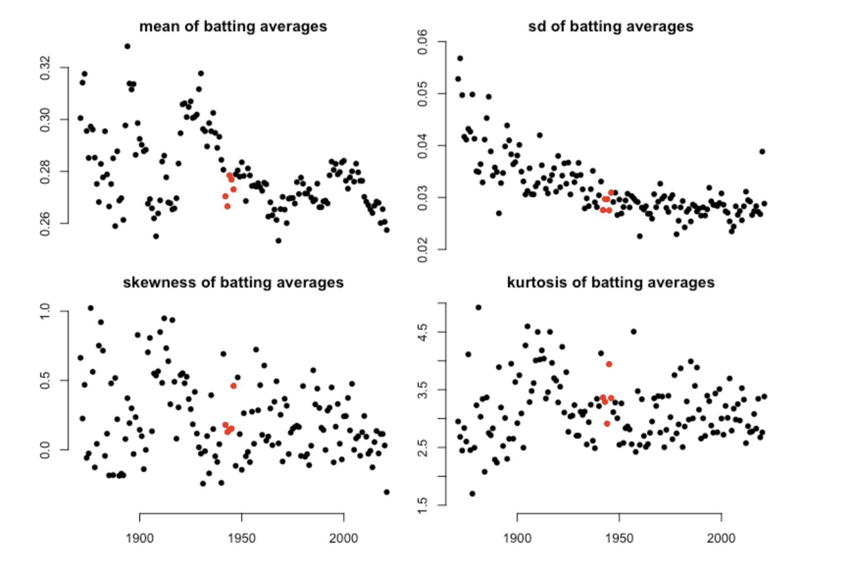
Figure 2: Four statistical moments of the batting average distribution from 1871 to 2021 season. Points in red correspond to seasons surrounding the peak of WWII (1941-1946)

To illustrate problems with the proxies in Berry et al. [1999], Schell [2013], Schell [2016], we will consider the distribution of batting averages over time with a focus on seasons surrounding the peak of World War II (WWII). About 71% of people MLB eligible population are removed from the major league due to WWII [Spoehr and Handy, 2018], and several top MLB players of the age served as soldiers. Thus the overall talent in the MLB was worse during WWII. However, a look at four statistical moments of the batting average distribution over time does not indicate any reduction in the talent of the MLB during WWII, see Figure 2.

The reason for this surprising observation is that baseball is a balance between hitting and pitching [Gould, 1996], and this balance was preserved during the WWII seasons. This balance poses challenges for the methodologies of Berry et al. [1999], Schell [2013] and Schell [2016]. It does not prove problematic for the Full House Model which directly incorporates the quality of the talent pool into its modeling framework.

rank	Peak in Full House	Career in Full House	Schell’s Method	Era-bridging Method	Raw Career
1	Ichiro Suzuki	Tony Gwynn	Tony Gwynn	Ty Cobb	Ty Cobb
2	Tony Gwynn	Rod Carew	Ty Cobb	Tony Gwynn	Rogers Hornsby
3	Mike Piazza	Ichiro Suzuki	Rod Carew	Ted Williams	Shoeless Joe Jackson
4	Nap Lajoie	Ty Cobb	Rogers Hornsby	Wade Boggs	Lefty O’Doul
5	Rod Carew	Jose Altuve	Stan Musial	Rod Carew	Ed Delahanty
6	Albert Pujols	Miguel Cabrera	Nap Lajoie	Shoeless Joe Jackson	Tris Speaker
7	Jose Altuve	Mike Trout	Shoeless Joe Jackson	Nap Lajoie	Billy Hamilton
8	Honus Wagner	Buster Posey	Honus Wagner	Stan Musial	Ted Williams
9	Josh Hamilton	Wade Boggs	Ted Williams	Frank Thomas	Dan Brouthers
10	Willie McGee	Roberto Clemente	Wade Boggs	Ed Delahanty	Babe Ruth
11	Tris Speaker	Vladimir Guerrero	Pete Browning	Tris Speaker	Dave Orr
12	Hank Aaron	Derek Jeter	Tris Speaker	Rogers Hornsby	Harry Heilmann
13	Ty Cobb	Mike Piazza	Mike Piazza	Hank Aaron	Pete Browning
14	Norm Cash	Robinson Cano	Dan Brouthers	Álex Rodríguez	Willie Keeler
15	Wade Boggs	Hank Aaron	Tip O’Neill	Pete Rose	Bill Terry
16	John Olerud	Matty Alou	Kirby Puckett	Honus Wagner	Lou Gehrig
17	Joe Torre	Shoeless Joe Jackson	Tony Oliva	Roberto Clemente	George Sisler
18	Daniel Murphy	Joe Mauer	Vladimir Guerrero	George Brett	Jesse Burkett
19	Cecil Cooper	Manny Mota	Mike Donlin	Don Mattingly	Tony Gwynn
20	Joe Mauer	Albert Pujols	Willie Keeler	Kirby Puckett	Nap Lajoie
21	Kirby Puckett	Dee Strange-Gordon	Edgar Martinez	Mike Piazza	Jake Stenzel
22	Magglio Ordonez	Edgar Martinez	Hank Aaron	Eddie Collins	Riggs Stephenson
23	Rogers Hornsby	Willie Mays	Derek Jeter	Edgar Martinez	Al Simmons
24	Robin Yount	Daniel Murphy	Joe DiMaggio	Paul Molitor	Cap Anson
25	Derek Jeter	Pete Rose	Babe Ruth	Willie Mays	John McGraw
pre-1950 in top 10:	2/10	1/10	7/10	6/10	10/10
pre-1950 in top 25:	5/25	2/25	15/25	10/25	24/25
proportion before 1950:	0.168	0.168	0.324	0.213	0.168
MLB eligible population:	(1871 - 2011)	(1871 - 2011)	(1876 - 1983)	(1901 - 1996)	(1871 - 2011)
chance in top 10:	1 in 1.92	1 in 1.19	1 in 60	1 in 113	1 in 55835085
chance in top 25:	1 in 2.42	1 in 1.06	1 in 242	1 in 38	1 in greater than $10^{12}$

Table 3: BA rankings from Full House Model, Era-bridging Method, and Schell’s Method. Players that started their careers before 1950 are indicated in bold text. The proportion before the 1950 row is the proportion of the MLB eligible population from the range in the MLB eligible population row that began their career before baseball was integrated. The upper range is chosen to reflect longevity, cut-offs, and design choices that were made by the authors of the considered methods. The chance in the top 10 or top 25 rows is computed as 1 divided by the probability of observing $x$ or more players who began their career before baseball was integrated, as calculated using the binomial distribution with respect to the success probability listed in the row labeled proportion before 1950.

	Career Full House	Schell’s Method	Raw Career
1	Barry Bonds	Ted Williams	Ted Williams
2	Joey Votto	Babe Ruth	Babe Ruth
3	Ted Williams	Rogers Hornsby	John McGraw
4	Nick Johnson	Barry Bonds	Billy Hamilton
5	Frank Thomas	John McGraw	Lou Gehrig
6	Jason Giambi	Billy Hamilton	Barry Bonds
7	Mickey Mantle	Topsy Hartsel	Bill Joyce
8	Edgar Martinez	Mel Ott	Rogers Hornsby
9	Babe Ruth	Roy Thomas	Ty Cobb
10	Lance Berkman	Mickey Mantle	Jimmie Foxx
11	Rickey Henderson	Wade Boggs	Tris Speaker
12	Manny Ramirez	Frank Thomas	Eddie Collins
13	Brian Giles	Lou Gehrig	Ferris Fain
14	Jim Thome	Rickey Henderson	Dan Brouthers
15	Chipper Jones	Stan Musial	Max Bishop
16	Jeff Bagwell	Edgar Martinez	Shoeless Joe Jackson
17	Wade Boggs	Ty Cobb	Mickey Mantle
18	Gene Tenace	Dan Brouthers	Mickey Cochrane
19	Miguel Cabrera	Tris Speaker	Mike Trout
20	Joe Mauer	Joe Cunningham	Frank Thomas
21	Bobby Abreu	George Gore	Edgar Martinez
22	Travis Hafner	Eddie Collins	Stan Musial
23	Justin Turner	Ross Youngs	Cupid Childs
24	John Olerud	Mike Hargrove	Wade Boggs
25	David Wright	Jeff Bagwell	Jesse Burkett
pre-1950 in top 10:	2/10	8/10	9/10
pre-1950 in top 25:	2/25	16/25	19/25
proportion before 1950:	0.168	0.267	0.168
MLB eligible population:	(1871 - 2011)	(1876 - 1993)	(1871 - 2011)
chance in top 10:	1 in 1.92	1 in 1477	1 in 1105124
chance in top 25:	1 in 1.06	1 in 9776	1 in 8.4 * $10^{9}$

Table 4: OBP rankings from Full House Model and Schell’s Method. Players that started their careers before 1950 are indicated in bold text. The proportion before the 1950 row is the proportion of the MLB eligible population from the range in the MLB eligible population row that began their career before baseball was integrated. The upper range is chosen to reflect longevity, cut-offs, and design choices that were made by the authors of the considered methods. The chance in the top 10 or top 25 rows is computed as 1 divided by the probability of observing $x$ or more players who began their career before baseball was integrated, as calculated using the binomial distribution with respect to the success probability listed in the row labeled proportion before 1950.

	Peak in Full House	Career in Full House	Era-bridging Method	PPS detrending Method	Peak in Schell	Career in Schell	Raw AB per HR
1	Frank Howard	Babe Ruth	Mark MeGwire	Babe Ruth	Barry Bonds	Babe Ruth	Mark McGwire
2	Willie Stargell	Mark McGwire	Juan Gonzalez	Mel Ott	Babe Ruth	Mark McGwire	Babe Ruth
3	Mark McGwire	Barry Bonds	Babe Ruth	Lou Gehrig	Mark McGwire	Ted Williams	Barry Bonds
4	Babe Ruth	Dave Kingman	Dave Kingman	Jimmie Foxx	Buck Freeman	Barry Bonds	Jim Thome
5	Pedro Alvarez	Willie Stargell	Mike Schmidt	Hank Aaron	Ed Delahanty	Mike Schmidt	Giancarlo Stanton
6	Khris Davis	Willie McCovey	Harmon Killebrew	Rogers Hornsby	Tim Jordan	Lou Gehrig	Ralph Kiner
7	Sammy Sosa	Mike Schmidt	Frank Thomas	Cy Williams	Willie Stargell	Harmon Killebrew	Harmon Killebrew
8	Ted Williams	Nelson Cruz	Jose Canseco	Barry Bonds	Rogers Hornsby	Jimmie Foxx	Sammy Sosa
9	Nelson Cruz	Harmon Killebrew	Ron Kittle	Willie Mays	Jim Thome	Dave Kingman	Ted Williams
10	Lou Gehrig	Darryl Strawberry	Willie Stargell	Ted Williams	Dave Kingman	Reggic Jackson	Manny Ramirez
11	Eddie Mathews	Mickey Mantle	Willie McCovey	Reggie Jackson	Roy Sievers	Bill Nicholson	Mike Trout
12	Willie Mays	Jim Thome	Darryl Strawberry	Mike Schmidt	Jeff Bagwell	Mickey Mantle	Adam Dunn
13	Albert Pujols	Ted Williams	Bo Jackson	Frank Robinson	Ted Williams	Ralph Kiner	Ryan Howard
14	Miguel Cabrera	David Ortiz	Ted Williams	Harmon Killebrew	Kevin Mitchell	Joe DiMaggio	Juan Gonzalez
15	Giancarlo Stanton	Jose Canseco	Ralph Kiner	Gavvy Cravath	Mike Schmidt	Willie Stargell	Dave Kingman
16	Mike Schmidt	Manny Ramirez	Pat Seerey	Honus Wagner	Lou Gehrig	Hack Wilson	Russell Branyan
17	Harmon Killebrew	Ryan Howard	Reggie Jackson	Willie McCovey	Fred Dunlap	Rogers Hornsby	Mickey Mantle
18	Mickey Mantle	Hank Sauer	Ken Griffey	Harry Stovey	Harry Stovey	Darryl Strawberry	Alex Rodriguez
19	Manny Ramirez	Gorman Thomas	Albert Belle	Ken Griffey Jr.	Charlie Hickman	Willie McCovey	Jimmie Foxx
20	Ralph Kiner	Ralph Kiner	Dick Allen	Stan Musial	Bill Nicholson	Glenn Davis	Mike Schmidt
21	Reggie Jackson	Sammy Sosa	Barry Bonds	Willie Stargell	Boog Powell	Wally Berger	Jose Canseco
22	Frank Thomas	Frank Howard	Dean Palmer	Eddie Murray	Joe DiMaggio	Eddie Mathews	Albert Belle
23	Barry Bonds	Eddie Mathews	Hank Aaron	Mark McGwire	Eddie Mathews	Harry Stovey	Khris Davis
24	Chris Davis	Oscar Gamble	Jimmie Foxx	Mickey Mantle	Mickey Mantle	Frank Howard	Ron Kittle
25	Alex Rodriguez	Glenn Davis	Mike Piazza	Al Simmons	Tris Speaker	Mel Ott	Carlos Delgado
pre-1950 in top 10:	3/10	1/10	1/10	7/10	5/10	4/10	3/10
pre-1950 in top 25:	4/25	4/25	5/25	12/25	13/25	12/25	4/25
proportion before 1950:	0.138	0.190	0.213	0.270	0.176	0.292	0.190
MLB eligible population:	(1871 - 2021)	(1871 - 2005)	(1901 - 1996)	(1871 - 1993)	(1876 - 2003)	(1876 - 1988)	(1871 - 2005)
chance in top 10:	1 in 6.68	1in 1.14	1 in 1.1	1 in 178	1 in 51	1 in 3.04	1 in 3.42
chance in top 25:	1 in 2.18	1 in 1.38	1 in 1.56	1 in 50.2	1 in 10381	1 in 28	1 in 1.38

Table 5: HR rankings from Full House Model, Era-bridging Method, Schell’s Method, and PPS Detrended Method. Players that started their careers before 1950 are indicated in bold text. The proportion before the 1950 row is the proportion of the MLB eligible population from the range in the MLB eligible population row that began their career before baseball was integrated. The upper range is chosen to reflect longevity, cut-offs, and design choices that were made by the authors of the considered methods. The chance in the top 10 or top 25 rows is computed as 1 divided by the probability of observing $x$ or more players who began their career before baseball was integrated, as calculated using the binomial distribution with respect to the success probability listed in the row labeled proportion before 1950.

4 Full House Modeling assumptions and data considerations

4.1 Historical MLB eligible population

We have taken the following three principal steps to construct the MLB eligible population. We first construct the list of countries comprising the MLB eligible population using Census counts and other domestic and international population data for baseball-age players. We include a country’s population of aged 20-29 year old males by year in the MLB eligible population when a person from that country reaches the MLB. Several countries that have produced two or more players will be added to the MLB eligible population [Baseball-Reference, 2022]. The countries that will form our MLB eligible population will be Aruba, Australia, Bahamas, Brazil, Canada, Colombia, Cuba, Curaçao, Dominican Republic, Jamaica, Japan, Mexico, Nicaragua, Panama, Puerto Rico, South Korea, Taiwan, the United States, the United States Virgin Islands, and Venezuela.

We have consulted the United States Census, Statistics Canada, United Nations population tables, and the World Bank to tally the MLB eligible population over time. We then attempt to weigh each year by each countries’ interest in baseball using polling sources [Fimrite, 1977, Baird, 2005, Schmidt and Berri, 2005, Burgos Jr, 2007, Jamail, 2008]. Finally, we have adjusted population sizes to account for the effects of wars, and the rates of integration in the two traditional leagues which comprise the MLB [Armour, 2007] among other adjustments. Specifics can be seen in the Supplementary Materials.

Table 6 shows the MLB eligible population throughout the years. As an example of how to interpret this dataset, consider the year 1950. There were 3.41 million eligible males aged 20-29. The proportion of the historical MLB eligible population that existed at or before 1950 is 0.141. We used the information in Table 6 to calculate the chances of observing $x$ players who began their career before 1950 in a top 10 and top 25 list using the testing procedure in Eck [2020a]. Population counts between the decades were calculated using interpolation.

year	population	cumulative population proportion
1870	0.39	0.004
1880	0.56	0.011
1890	0.67	0.019
1900	0.79	0.028
1910	1.27	0.042
1920	1.05	0.054
1930	1.36	0.070
1940	2.82	0.102
1950	3.41	0.141
1960	5.62	0.205
1970	7.80	0.294
1980	9.30	0.400
1990	8.18	0.494
2000	14.14	0.655
2010	14.50	0.820
2020	15.73	1.000

Table 6: MLB eligible population throughout the years. The 1st column indicates the year; 2nd column indicates the estimated eligible population size(in millions) and the 3rd column indicates the proportion of the MLB eligible population in row $x$ that was eligible at or before row $x$.

4.2 Full House Modeling assumptions and specifications

In Section 2 we supposed that the all $N_{i}$ individuals in population $i$ have talents $X_{i,1},\ldots,X_{i,N_{i}}\overset{iid}{\sim}F_{X}$. Here $N_{i}$ corresponds to the number of MLB eligible males aged 20-29. The Full House Model results displayed throughout Section 3 assumed that $F_{X}$ corresponds to a Pareto($\alpha$) distribution with $\alpha=\log_{4}5\approx 1.16$. This choice of $\alpha$ reflects the Pareto principle or “80-20 rule” [Pareto, 1964]. Berri and Schmidt [2010] noted that the superstars are really important for their teams to win and state that about 80% of wins appear to be produced by the top 20% of players. Thus there is some precedent for our assumption on $F_{X}$. In Section 5 we perform a sensitivity analysis on choices of $F_{X}$. This sensitivity analysis reveals that our conclusions do not strongly depend on the distribution assumed for $F_{X}$. Specific rankings may undergo minor influences as a result of choices of the distribution assumed for $F_{X}$, but the top-end players are not sensitive to such choices and there is considerable overlap of the players listed among the top 10 or top 25 lists corresponding to different choices of distributions assumed for $F_{X}$.

The Full House Model results displayed throughout Section 3 had placed era-adjusted baseball careers within a common context. Namely, every player’s career was computed as if it began in 1977. Thus steps 1-3 of the algorithm in Section 2.4 were applied to every MLB player’s first MLB season and steps 4-6 of the algorithm in Section 2.4 found era-adjusted statistics within the context of the 1977 MLB season, steps 1-3 of the algorithm in Section 2.4 were applied to every players’ second MLB season and steps 4-6 of the algorithm in Section 2.4 found era-adjusted statistics within the context of the 1978 MLB season, and so on. The rationale for our choice to start era-adjusted careers in 1977 is presented in a sensitivity analysis in Section 5. This sensitivity analysis reveals that our conclusions do not strongly depend on the common context in which we choose to evaluate careers. Specific rankings may undergo minor influences resulting from a particular choice, but the top-end players are not sensitive to such choices. Ranges for rankings across contexts are also presented in Section 5.

4.3 Considerations for batting statistics

In this section, we detail the considerations made for the batting statistics that we era-adjust using the Full House Model: batting average (BA), hits (H), home runs (HR), walks (BB), on base percentage (OBP), bWAR, and fWAR. We also adjust at-bats (AB) and plate appearances (PA) to accommodate changing season lengths throughout baseball’s history.

Park factor adjustments are also considered in our model and we apply the adjusted park index from Schell [2016] to all ballparks from the 1871 season to the 2021 season. BA and HR are two statistics that can be affected by the ballpark and we apply the park factor adjustment to these two statistics, which account for the handedness of batters.

The Full House Model will only be applied to the statistics obtained by full-time players. We define the full-time hitter cutoff as the median PAs after screening out hitters who appeared in fewer than 75 PAs. This criterion is flexible enough to account for changing the number of games played over time as well as seasons shortened by labor strikes and pandemics.

We will use parametric distributions as in Section 2.1 to measure the BA since it is widely recognized that the BA follows a normal distribution [Gould, 1996]. We perform a Shapiro-Wilk’s test [Shapiro and Wilk, 1965] of normality on the BA distribution for each season, and the $p$-values of BA in 121 seasons out of a total of 151 seasons are greater than 0.05. Figure 3 displays estimated BA from Full House Model using the parametric and nonparametric approaches. We see that there is not much difference between these approaches.

We will use nonparametric methods as in Section 2.2 to measure HR, BB, bWAR, and fWAR since these statistics have not been demonstrated to follow any common distribution we know. We also use HR per AB, BB per AB, bWAR per game, and fWAR per game as the components in the system to compute the talent scores.

Instead of using the raw games in the dataset, we calculate mapped games by applying quantile mapping. Quantile mapping is based on the idea that a $p$th percentile player’s games in one year are equal to a $p$th percentile player’s games in another year. AB and PA also change across baseball history as the number of games and the walk rate change. We calculate adjusted-AB as:

$$\textrm{adjusted-AB}=\textrm{mapped-PA - adjusted-BB - HBP - SH - SF},$$ (8)

where HBP, SH, and SF are short for, respectively, hit by pitch, sacrifice hits, and sacrifice flies. We assume that these values do not change over time, and mapped-PA is computed similarly as mapped games.

From here, era-adjusted hits, walks, and home runs can be computed from the per AB rates and (8) and mapped-PAs. For example, era-adjusted hits is equal to era-adjusted batting average multiplied by adjusted-AB. Era-adjusted bWAR or fWAR are obtained by multiplying era-adjusted bWAR per game or fWAR per game with mapped games. We also compute era-adjusted OBP as

$$\textrm{adjusted-OBP}=\frac{\textrm{adjusted-BA * adjusted-AB + adjusted-BB + HBP}}{\textrm{adjusted-AB + adjusted-BB + HBP + SF}}.$$ (9)

We find that some players’ statistics are very volatile. For example, some players’ performance will fall considerably as a result of injury, and the player will rebound as they recover. This volatility can be overly exaggerated by the Full House Model, especially for older era players. To solve this, we apply natural cubic spline smoothing to alleviate these dramatic variations. The natural cubic spline method was determined to have a minimal bias when compared with local polynomial regression fitting. We report the average of the raw era-adjusted statistics and the smoothed era-adjusted statistics. This was done in order to not smooth over rarified outlying achievement.

We also find that the Full House Model can harshly punish the tails of players’ careers, especially for older era players. This is due to players reaching or staying in the MLB during a less talented era of baseball history, and having these seasons translate to terrible play in the common context that we judge all players. For example, a late-career declined in the 1910s would correspond to a player who would likely be out of the MLB in the 1980s. To alleviate this problem, we trim players’ careers when their era-adjusted WAR falls below zero. This trimming method is as follows: First, we remove the bad players who have not made any positive contributions to the team wins. Then we detect the numbers of bad performance seasons that their WARs (bWAR or fWAR) are below 0 at both tails of their careers. For the starting seasons of their career, bad performance seasons are trimmed except for the season that just before the season they make positive contributions to the team wins. For the end-of-seasons of their career, bad performance seasons are trimmed except for the one or two seasons that just after the season they make positive contributions to the team wins.

Era-adjusted batting statistics obtained from the Full House Model are seen in Table 9 and 10 in the Appendix.

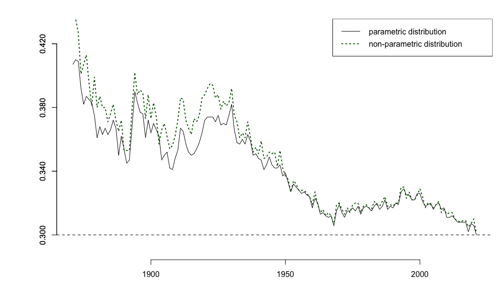
Figure 3: Estimated batting averages from the Full House Model using parametric and nonparametric estimation over time. The batting average plot shows the estimated batting average over time for a hypothetical .300-batter in 2021.

4.4 Considerations for pitching statistics

In this section, we detail the considerations made for the pitching statistics that we era-adjust using the Full House Model: earned-run average (ERA), strikeouts (SO), bWAR, and fWAR. We also adjust innings pitched (IP) using a similar quantile mapping approach that we applied to Game or PA for batters. We will use nonparametric methods as in Section 2.2 to measure these pitching statistics since these statistics have not been demonstrated to follow any common distribution we know. Note that smaller values of ERA are better, so we apply the Full House Model to the negation of ERA. Smoothing and career trimming were applied to era-adjusted pitching statistics in the same way as to batting statistics.

It is necessary to define the full-time pitchers, as the deployment of pitchers changes significantly in different eras. We define full-time pitchers as the pitchers who are most innings pitched and the full-time pitchers’ cutoff can be calculated as follow: We first compute the number of average starting pitchers by measuring the average rotation size for each team and then multiply it by the number of teams in each season as the number of average starting pitchers in that season. Then the number of full-time pitchers is equal to the number of average starting pitchers.

We also adjust for the difference in pitching rotation sizes across eras. The average rotation size for each team can be calculated as the largest number of unique starting players within a moving window of consecutive games. The size of the moving window stops increasing when the number of unique starting players in this moving window is smaller than the size of the moving window. Then we take the average of the numbers we compute as the window moves and consider it as the average rotation size for each team.

We now introduce an adjustment for pitching statistics based on different rotation sizes. The idea is that pitchers from an era with smaller rotation sizes would have better statistics as judged against their peers had they played in a year with a larger rotation size. We give an example of how our adjustment works: the average rotation size was three pitchers in 1984. Supposed that the projected season has an average rotation size of five starting pitchers with 30 teams in the league. Therefore we add the minimum seasonal talent score for a hypothetical rotation size equal to that of the pitcher’s context to the computed un-adjusted talent score of that pitcher. In other words, the 3*30 = 90th qualifying starter’s talent score in the projected season is added to the talent score of the pitchers from the 1894 season in which the average rotation size is three.

Similarly, we deduct some points to starting pitchers who played in the season in which average rotation sizes were larger than the rotation of any season that we project into. For example, we assume that a pitcher played in the 2021 season in which the average rotation size is five. Supposed that the projected season has an average of three starting pitchers with 12 teams, then some pitchers that are chosen as starting pitchers in the 2021 season perform badly in the projected season since they are not in a rotation. Therefore the 5*12 = 60th qualifying starter’s talent score in the projected season is deducted from the talent score of the pitchers from the 2021 season in which the average rotation size is five.

Era-adjusted pitching statistics obtained from the Full House Model are seen in Table 11 and Table 12 in the Appendix.

5 Validation and Sensitivity Analyses

In this section, we validate our model to ensure the appropriateness of the assumption that the talent-generating process is Pareto distribution with parameter $\alpha=1.16$ via a sensitivity analysis simulation. The goal of this analysis is to determine how many of the top 25 talented players by BA our method can correctly identify under a variety of simulation configurations, some of which are chosen to stretch the credibility of our method.

In each simulation, we first randomly generate samples from four different talent generation distributions, which are Pareto distribution with parameter $\alpha=1.16$ (i.e. the talent generating process is correctly specified), Pareto distribution with parameter $\alpha=3$, folded normal distribution with parameters $\mu=0,\sigma=1$, and standard normal distribution. Within each talent generation distribution, we vary the MLB eligible population sizes $N_{i}$ for five different hypothetical leagues. Details of the simulation information are in the Table 13. Then we select 300 items with the largest talents in each dataset and consider them as the full-time batters in MLB. Therefore, $n_{i}=300$ for all $i$. We will generate BA from the talent scores using a normal distribution with parameters Table 13. For each league $i$, these values are generated as

$$Y_{i,(j)}=F_{Y_{i}}^{-1}\left(F^{-1}_{U_{i,(j)}}\left(F_{X_{i,(N_{i}-n_{i}+j)}}(X_{i,N_{i}-n_{i}+j})\right)|\theta_{i}\right),$$

where $\theta_{i}$ are the parameters for the normal distribution, and our choices for these parameters reflect the shrinking BA variability that has been observed over time [Gould, 1996].

We apply the Full House Model with $F_{X}$ assumed to be Pareto with $\alpha=1.16$ to this generated data, and investigate how well the Full House Model correctly identifies the top 25 players as judged by talent scores. We also consider misspecification in the estimation of the MLB eligible population size. We consider two underestimations of the MLB eligible population where 1) the estimation improves as time increases and 2) the underestimation deteriorates as time increases. This configuration was chosen to be deliberately antagonistic to our method, especially when the talent-generating process was misspecified. The details of the information are in the Table 13. We also compare our Full House Model to rankings based on Z-scores and unadjusted BA. Z-scores are a building block for Schell’s method.

200 Monte Carlo iterations of our simulation are performed and the results are depicted in plot 4 and Table 7. What we found is that our Pareto assumption with $\alpha=1.16$ holds up well even when the talent-generating process and the MLB eligible population is not correctly specified. Moreover, our method correctly identifies more top-25 talented players than both Z-scores and raw unadjusted batting averages.

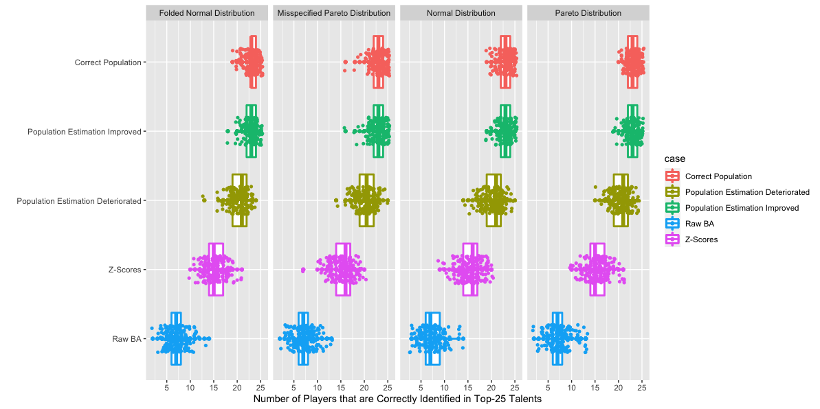
Figure 4: Monte Carlo simulation investigating the number of correctly identified talents in a top-25 list under four different latent talent distribution $F_{X}$. Each column of the plot indicates a different talent generation distribution. The first three rows of the plot are variants of our Full House Model where $F_{X}$ is assumed to be Pareto with $\alpha=1.16$. The first row displays the performance of our method with the MLB eligible population correctly estimated. The second and third rows display the performance of our method with the MLB eligible population incorrectly estimated. In the second row, we underestimate the MLB eligible population where the estimation improves as time increases. In the third row, we underestimate the MLB eligible population where the estimation deteriorates as time increases. The fourth row displays the performance of Z-scores and the fifth row displays the performance of raw unadjusted batting averages

That being said, there is considerable overlap between the box plot in the second row and the box plot in the fourth row. This suggests that Z-scores may not be strictly worse than our method under misspecification. A more detailed look shows that this is not the case. During each simulation, we directly compare our method when the underestimation estimation of the MLB eligible population deteriorates and Z-scores (third and fourth rows of Figure 4). Then we calculate the proportion of simulations that our model with the population estimation deteriorates strictly beats the Z-scores method and either beats or ties the Z-scores method. Table 7 indicates that our Full House Model is almost strictly better than the Z-scores method in each simulation. Thus, the Full House Model performs better than Z-scores even when $F_{X}$ and the estimated eligible population sizes are badly misspecified.

	Correct Pareto distribution	Incorrect Pareto distribution	Normal distribution	Folded normal distribution
beats or ties	1	1	1	1
strictly beats	1	1	0.995	1

Table 7: Compare the results between Full House Model with the population estimation deteriorated and Z-scores

We also validate the stability of rankings across different starting years, and we demonstrate why we choose 1977 as the starting year for comparing career trajectories. We investigated 50 similar trajectories computed with starting years from 1946 to 1995 and calculated the career bWAR rankings for the top players. The inner 80% range of bWAR rankings is depicted in Figure 5. The ordering of names on the y-axis corresponds to the rankings given by the trajectory that starts in 1977. We see that the 1977 rankings fall within the range of rankings computed from the 49 other trajectories which makes it a good candidate starting point. We also investigated single-season reference years instead of trajectories. This method is much less stable as the balance between hitting and pitching and the distribution of bWAR are more variable. Thus we went with trajectories and choose 1977 as the starting year. Figure 5 indicates very stable rankings for those appearing in the top 10 with greater stability at the top of the list.

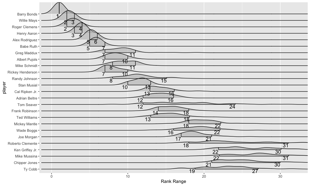
Figure 5: Top 25 batters’ inner 80% range of bWAR rankings that trajectory starts in 1977 and density function of bWAR rankings from 50 trajectories with starting years from 1946 to 1995.

Also, we validate the stability of rankings when we change the latent distribution $F_{X}$ to a folded normal distribution, the Pareto distribution with $\alpha=3$, and the standard normal distribution. The table below shows the rankings with these three different latent talent distributions. Compared to results from the Pareto distribution with $\alpha=1.16$ in the Full House Model, the assumed latent talent distribution $F_{X}$ does not greatly influence the results

	Standard normal	Folded normal $(\mu=0,\sigma=1)$	Pareto with $\alpha=3$	Pareto with $\alpha=1.16$
1	Barry Bonds	Barry Bonds	Barry Bonds	Barry Bonds
2	Willie Mays	Willie Mays	Willie Mays	Willie Mays
3	Roger Clemens	Roger Clemens	Roger Clemens	Roger Clemens
4	Hank Aaron	Hank Aaron	Hank Aaron	Hank Aaron
5	Alex Rodriguez	Babe Ruth	Babe Ruth	Alex Rodriguez
6	Babe Ruth	Alex Rodriguez	Alex Rodriguez	Babe Ruth
7	Greg Maddux	Greg Maddux	Cy Young	Greg Maddux
8	Albert Pujols	Albert Pujols	Greg Maddux	Albert Pujols
9	Mike Schmidt	Mike Schmidt	Walter Johnson	Mike Schmidt
10	Rickey Henderson	Rickey Henderson	Albert Pujols	Rickey Henderson
11	Randy Johnson	Randy Johnson	Mike Schmidt	Randy Johnson
12	Stan Musial	Stan Musial	Rickey Henderson	Stan Musial
13	Tom Seaver	Cy Young	Tom Seaver	Cal Ripken Jr.
14	Cal Ripken Jr.	Tom Seaver	Randy Johnson	Adrian Beltre
15	Adrian Beltre	Cal Ripken Jr.	Stan Musial	Tom Seaver
16	Frank Robinson	Adrian Beltre	Cal Ripken Jr.	Frank Robinson
17	Ted Williams	Frank Robinson	Adrian Beltre	Ted Williams
18	Cy Young	Ted Williams	Frank Robinson	Mickey Mantle
19	Mickey Mantle	Walter Johnson	Ted Williams	Wade Boggs
20	Wade Boggs	Mickey Mantle	Mickey Mantle	Joe Morgan
21	Joe Morgan	Wade Boggs	Bert Blyleven	Roberto Clemente
22	Roberto Clemente	Joe Morgan	Wade Boggs	Ken Griffey Jr.
23	Walter Johnson	Roberto Clemente	Joe Morgan	Mike Mussina
24	Ken Griffey Jr.	Ken Griffey Jr.	Lefty Grove	Chipper Jones
25	Mike Mussina	Mike Mussina	Roberto Clemente	Ty Cobb
matched names in top 10	10/10	10/10	8/10
matched ranks in top 10	10/10	8/10	4/10
matched names in top 25	23/25	23/25	21/25
matched ranks in top 25	14/25	10/25	4/25

Table 8: bWAR rankings from Full House Model using folded normal distribution, Pareto distribution with $\alpha$ = 3, and standard normal distribution as the latent talent distribution $F_{X}$. Players that started their careers before 1950 are indicated in bold text. The last four rows show the numbers of matched names and rank in the top 10 and top 25 lists compared with the Pareto distribution with $\alpha$ = 1.16

6 Summary and Discussion

In this article, we develop a model motivated by Stephen J. Gould’s book Full House: The Spread of Excellence from Plato to Darwin [Gould, 1996] for making statistical inference on cross-system components. We apply this model to several important statistics in baseball including era-adjusted career statistics, where all players’ statistics are evaluated in the same historical context. Our results challenge an established consensus of greatness in baseball which we argue resulted from nostalgic bias and statistical methods that do not take into account the evolution of baseball. We reinforce this claim by showing that our method produces ranking lists which align with what would be expected under a practical assumption that baseball talent is evenly distributed across time. Existing methods over-included baseball players that played before baseball was integrated into their ranking of the game’s greatest players.

Stephen Jay Gould was not quiet about assumptions about the distribution of talent. At various points throughout Chapter 7 in Full House: The Spread of Excellence from Plato to Darwin, Gould said:

“The first explanation [for the disappearance of 0.400 hitting] invokes the usual mythology about good old days versus modern mollycoddling, Nintendo, power lines, high taxes, rampant vegetarianism, or whatever contemporary ill you favor for explaining the morally wretched state of our current lives. In the good old days when men were men, chewed tobacco, and tormented homosexuals with no fear of rebuke, players were tough and fully concentrated. They did nothing but think baseball, play baseball, and live baseball… I call this version [explanation] the Genesis Myth to honor the appropriate biblical passage about wondrous early times: “There were giants in the earth in those days” (Genesis 6:4)… In his 1986 book, The Science of Hitting, [Ted] Williams … explicitly embraced postulates of the Genesis Myth by stating that, since baseball hadn’t altered in any other way, the decline of high hitting must record an absolute deterioration of batting skills among the best.”

Gould states that this Genesis Myth is a part of a chorus of woe that sings a foolish tune that need not long detain us [Gould, 1996]. Yet the Genesis Myth is alive and well decades after Gould’s book was first printed. In 2022, ESPN analyst Jeff Passan felt the need to “stand up for the legacy of Babe Ruth” by saying “this is a guy who hit more home runs than entire teams” and followed that with “I understand that Willie Mays was better than his peers, Babe Ruth was better than the sport” . While it is true that Ruth hit more home runs than entire teams, Passan is attributing this accomplishment to Babe Ruth with no mention that players of his era simply did not try to frequently hit home runs. That Babe Ruth hit more home runs than entire teams is somehow an indicator of his singular grand talent is just the Genesis Myth. The ESPN list is presented in Table 2, and one can see that they list Babe Ruth as the greatest player ever. We can also see from Table 2 that ESPN has, yet again, included too many pre-integration players in their list of great players [Eck, 2020a, b].

The Genesis Myth is not just being advanced by media pundits like Jeff Passan. This myth is present within the methodologies of Petersen et al. [2011] and Petersen and Penner [2020]. These authors presented a spurious narrative of baseball history in which modern players are the beneficiaries of several technological advantages and performance-enhancing drugs (PEDs), and these benefits are what have inflated our perceptions of their talent. In Petersen et al. [2011], they said:

“While there is much speculation and controversy surrounding the causes for changes in player ability, we do not address these individually. In essence, we blindly account for not only the role of PED but also changes in the physical construction of bats and balls, sizes of ballparks, talent dilution of players from expansion, etc… We demonstrate the utility of our detrending method by accounting for the changes in player performance over time in professional baseball, which is particularly relevant to the induction process for HOF and to the debates regarding the widespread use of PED in professional sports… Hence, the raw accomplishments of sluggers during the steroids era will naturally supersede the records of sluggers from prior eras. So how do we ensure that the legends of yesterday do not suffer from historical deflation?”

These authors do not mention racial integration or a general increase in the eligible population as something to take into account, yet they mention talent dilution of players from expansion. Petersen and Penner [2020] repeated this spurious narrative.

Eck [2020a] commented that these authors (in response to Petersen et al. [2011], although the same is applicable for Petersen and Penner [2020]) “misunderstand the effect of talent dilution from expansion and ignore reality. The talent pool was more diluted in the earlier eras of baseball than now because of a relatively small eligible population size and the exclusion of entire populations of people on racial grounds.”

Alexander M. Petersen, the lead author of Petersen et al. [2011] and Petersen and Penner [2020], was interviewed for a BU Today article [Johnson, 2011] which contained the passage:

“Players like Babe Ruth, Lou Gehrig, and Ted Williams shoot up the list because they were giants in their own era as well as across the decades. Petersen says his approach is a way to make the statistics fairer: besides accounting for the possible effects of steroids, detrending allows for changes in equipment, diet, conditioning, and even medical procedures like Tommy John surgery (replacing a ligament in the elbow with a tendon to lengthen a pitching career), all of which have changed the game since Ruth’s time.”

It is clear that Petersen et al. [2011] and Petersen and Penner [2020] are influenced by the Genesis Myth, and it is unconscionable how any discussion of making baseball statistics fairer would not mention the racial segregation that existed in baseball from the late 1880s to 1947. In fact, the phrases “integration” or “segregation” are only mentioned once between all of Petersen et al. [2011], Johnson [2011], and Petersen and Penner [2020]. It seems that these authors view racial integration of baseball as a footnote, something that is worth passing mention but did not dramatically alter the composition of talent in the MLB. Unsurprisingly, these authors’ methodology includes an over-representation of players from the past in their all-time home run rankings, see Table  5.

Extensive criticisms of the methodology of Petersen et al. [2011] and Petersen and Penner [2020] can be found in Eck [2020a] and Eck [2020b]. Most notable of these criticisms is a conflation that these authors make between “renormalization” and stationarity. In Petersen and Penner [2020] they said: “notably, as a result, and consistent with a stationary data generation process, the league averages are more constant over time after renormalization, thereby demonstrating the utility of these renormalization methods to standardize multi-era individual achievement metrics.” The renormalization process in Petersen and Penner [2020] involves the detrending of seasonal averages, no other statistical moments are considered. In Eck [2020b] it is argued that the detrending of seasonal averages influences the variance in a way that prioritized players who began their career before baseball was integrated.

The era-bridging method of Berry et al. [1999] does not fall prey to the Genesis Myth to the same degree as Petersen et al. [2011] and Petersen and Penner [2020]. They did, however, state that “Baseball has remained fairly stable within the United States, where it has been an important part of the culture for more than a century.” This rationale completely ignored the racial segregation that has plagued U.S. professional baseball throughout its history.

Michael Schell went to great lengths to compare batters across eras in two books, Schell [2013] and Schell [2016]. Motivated by Gould [1996], Schell also considered the standard deviation as a proxy for measuring a changing talent pool. He said, “we will call the season standard deviation of the park-adjusted average the performance spread, and will use it as a measure of the talent pool.” On page 58 in Schell [2016], he outlined some problems with his standard deviation approach:

“Someday we will need to abandon the use of the standard deviation as a talent pool adjustment altogether and search for another talent pool adjustment method, likely involving more difficult statistical methods than those used in this book.”

We advocate for our Full House Model as an answer to Schell’s call for a method that adjusts for the changing talent pool in a more appropriate manner than the standard deviation. The Full House Model directly incorporates the quality of the talent pool as a central modeling component. We applaud Michael Schell for his comprehensive adjustments and note that we use his park-factor adjustments in our work.

In the future, one may extend our model to the multivariate Full House Model using multivariate order statistics and multivariate empirical distribution, and make statistical inferences on cross-system multi-dimensional components. It would be helpful to compare batter’s talent by using several batting statistics jointly. In our model, we assume statistics are independent across years. This is not correct and we knowingly add smoothing to alleviate shortcomings with the independence assumption. A Full House Model that can integrate trajectories for players’ careers in its construction would alleviate the shortcomings of our independence assumption.

The Full House Model can be applied to other sports with different histories than baseball to obtain era-adjusted rankings. More generally, the Full House Model is appropriate for ranking lists where the components that are being compared undergo tractable changes in their quality. One interesting avenue for future work is using the Full House Model to era-adjust the rankings of memorable people provided by the Pantheon project [Yu et al., 2016].

We can see that great African American and Latin American players sit atop the era-adjusted WAR rankings. Moreover, it is not just one guy up top, it is four! Barry Bonds, Willie Mays, Hank Aaron, and Alex Rodriguez. This constitutes an important reversal in who we idolize as the pinnacle of achievement. The greatest athletic prowess that should be emulated is that of the best African American and Latin American ball players. Even if one “accounts for steroids” and removes Bonds and Rodriguez from consideration, then it’s still Mays and Aaron. Willie Mays and Hank Aaron are the players who, in fact, played the game the right way and in the era when MLB had opened up to all interested in playing America’s game.

7 Appendix

7.1 Details for calculating $Y^{*}$, $Y^{**}$, and $k$.

Based on the extreme value theory, see Castillo [2012] and induction from Scholz [1995], we would expect the $Y_{1},\dots,Y_{k}$ to show a approximately linear pattern with the log odds ratio of $p_{1},\dots,p_{k}$ when the extreme-value index $c$ is equal to 0, and the $Y_{1},\dots,Y_{k}$ to show a approximately linear pattern with $f_{c}(p_{1}),\dots,f_{c}(p_{k})$ when $c$ is not equal to 0, where $k$ is the data values in the tail of the distribution to use in the linear approximation, $p_{i}=p_{i,\gamma,n}$, and

$$f_{c}\left(p_{i}\right)=\frac{\left(-n\ln\left(p_{i}\right)\right)^{-c}-1}{c}$$ (10)

The extreme-value index c can be estimated from the data directly by using the moment estimate proposed by Dekkers et al. [1989], which is

$$\widehat{c}_{k}=M_{1,k}+1-.5\left(1-\frac{M_{1,k}^{2}}{M_{2,k}}\right)^{-1}$$ (11)

with

$$M_{1,k}=\frac{1}{k-1}\sum_{i=1}^{k-1}\log\left(\tilde{Y}_{i}/\tilde{Y}_{k}\right)\quad\text{ and }\quad M_{2,k}=\frac{1}{k-1}\sum_{i=1}^{k-1}\left[\log\left(\tilde{Y}_{i}/\tilde{Y}_{k}\right)\right]^{2},$$

$\text{ where }\tilde{Y}_{i}=Y_{i}-\operatorname{median}\left(X_{1},\ldots,X_{n}\right)$

An issue, that has not yet been addressed, is the number $k$ of data values in the tail of the distribution to use in the linear approximation step. Scholz [1995] shows that the k can be found in $[K_{1},K_{2}]$ and satisfies $T_{k}\in\left[\kappa_{k}t_{k-2,1/\kappa}(.25),\quad\kappa_{k}t_{k-2,1/\kappa}(.75)\right]$, where $K_{1}=\max(6,\lfloor 1.3\sqrt{n}\rfloor)$, $K_{2}=2\left\lfloor\log_{10}(n)\sqrt{n}\right\rfloor$, $T_{k}=\kappa_{k}t_{k-2,1/\kappa_{k}}$, and $\kappa_{k}$ is the standard deviation of the slope parameter in the generalized linear model. Then we choose the value $k$ so that the linear model or linear quadratic model fits the data best by comparing the adjusted R squared values. Then we can estimate the hypothetical cumulative probability at the maximum of components. After that, the $Y^{**}$ can be estimated by computing the value that satisfies the $\tilde{F}_{Y}(t)$ in Equation (3) at the maximum of components equals to the hypothetical cumulative probability that obtains before.

7.2 Mathematical details

Proof of Proposition 2.1:

Proof.

We will prove this result in cases. First, when $t\leq\widetilde{Y}_{i,(1)}$ or $t\geq\widetilde{Y}_{i,(n+1)}$ we have that $\mid\widetilde{F}_{Y}(t)-$ $\widehat{F}_{Y}(t)\mid=0.$ For any $j=1,\ldots,n$ and $\tilde{Y}_{i,(j)}\leq t<Y_{i,(j)},$ we have

$$\left|\widehat{F}_{Y}(t)-\widetilde{F}_{Y}(t)\right|=\left|\frac{j-1}{n}-\frac{j-1+\left(t-\widetilde{Y}_{i,(j)}\right)/\left(\tilde{Y}_{i,(j+1)}-\tilde{Y}_{i,(j)}\right)}{n}\right|\leq\frac{1}{n}$$

For any $j=1,\ldots,n$ and $Y_{i,(j)}<t<\tilde{Y}_{i,(j+1)},$ we have

$$\left|\widehat{F}_{Y}(t)-\widetilde{F}_{Y}(t)\right|=\left|\frac{j}{n}-\frac{j-1+\left(t-\tilde{Y}_{i,(j)}\right)/\left(\tilde{Y}_{i,(j+1)}-\tilde{Y}_{i,(j)}\right)}{n}\right|\leq\frac{1}{n}$$

Our conclusion follows. ∎

Proof of Corollary 2.1.1:

Proof.

We have, $\sup_{t\in\mathbb{R}}\left|\widetilde{F}_{Y}(t)-F_{Y}(t)\right|\leq\sup_{t\in\mathbb{R}}\left|\widetilde{F}_{Y}(t)-\widehat{F}_{Y}(t)\right|+\sup_{t\in\mathbb{R}}\left|\widehat{F}_{Y}(t)-F_{Y}(t)\right|.$ The conclusion follows from the Glivenko-Cantelli Theorem and Proposition 2.1. ∎

7.3 Era-Adjusted Hypothetical Career Statistics Based on Full House Model

	name	BA	name	OBP	name	HR
1	Tony Gwynn	0.343	Mike Trout	0.442	Hank Aaron	714
2	Rod Carew	0.327	Barry Bonds	0.437	Barry Bonds	714
3	Ichiro Suzuki	0.327	Joey Votto	0.437	Babe Ruth	706
4	Ty Cobb	0.325	Ted Williams	0.436	Albert Pujols	660
5	Jose Altuve	0.322	Frank Thomas	0.423	Willie Mays	607
6	Miguel Cabrera	0.319	Jason Giambi	0.422	Alex Rodriguez	597
7	Mike Trout	0.319	Mickey Mantle	0.422	Mike Schmidt	561
8	Buster Posey	0.318	Edgar Martinez	0.420	Frank Robinson	547
9	Wade Boggs	0.317	Babe Ruth	0.419	Ken Griffey Jr.	541
10	Roberto Clemente	0.317	Lance Berkman	0.418	David Ortiz	538
11	Vladimir Guerrero	0.316	Bryce Harper	0.418	Willie Stargell	526
12	Derek Jeter	0.316	Rickey Henderson	0.415	Mickey Mantle	518
13	Mike Piazza	0.315	Manny Ramirez	0.414	Jim Thome	517
14	Robinson Cano	0.314	Brian Giles	0.411	Reggie Jackson	513
15	Hank Aaron	0.313	Jim Thome	0.411	Eddie Mathews	513
16	Matty Alou	0.312	Chipper Jones	0.410	Eddie Murray	510
17	Shoeless Joe Jackson	0.312	Christian Yelich	0.410	Manny Ramirez	508
18	Joe Mauer	0.312	Freddie Freeman	0.409	Ted Williams	506
19	Manny Mota	0.312	Paul Goldschmidt	0.409	Miguel Cabrera	500
20	Albert Pujols	0.312	Jeff Bagwell	0.408	Rafael Palmeiro	498
21	José Abreu	0.311	Wade Boggs	0.408	Sammy Sosa	495
22	Dee Strange-Gordon	0.311	Gene Tenace	0.407	Willie McCovey	493
23	Edgar Martinez	0.311	Kris Bryant	0.406	Mark McGwire	485
24	Willie Mays	0.311	Miguel Cabrera	0.406	Harmon Killebrew	482
25	Daniel Murphy	0.311	Joe Mauer	0.406	Frank Thomas	474
pre-1950 in top 10:	1/10		2/10		1/10
pre-1950 in top 25:	2/25		2/25		2/25
MLB eligible population:	(1871 - 2011)		(1871 - 2011)		(1871 - 2005)
proportion before 1950:	0.168		0.168		0.190
chance in top 10:	1 in 1.19		1 in 1.92		1 in 1.14
chance in top 25:	1 in 1.06		1 in 1.06		1 in 1.04

Table 9: Top 25 BA, OBP, and HR leaders for MLB batters with era-adjusted hypothetical careers start at the 1977 season. Minimum career 3000 adjusted AB is required for BA and OBP. Batters who started their careers before 1950 are highlighted in the table. The proportion before the 1950 row is the proportion of the MLB eligible population from the range in the MLB eligible population row that began their career before baseball was integrated. The upper range is chosen to reflect longevity and cut-offs. The chance in the top 10 or top 25 rows is computed as 1 divided by the probability of observing $x$ or more players who began their career before baseball was integrated, as calculated using the binomial distribution with respect to the success probability listed in the row labeled proportion before 1950.

	name	ebWAR	name	efWAR
1	Barry Bonds	154.80	Barry Bonds	152.69
2	Willie Mays	145.47	Willie Mays	138.04
3	Hank Aaron	129.65	Hank Aaron	125.00
4	Alex Rodriguez	121.01	Alex Rodriguez	116.66
5	Babe Ruth	111.25	Babe Ruth	109.95
6	Albert Pujols	111.03	Mike Schmidt	107.80
7	Mike Schmidt	110.43	Rickey Henderson	106.86
8	Rickey Henderson	107.79	Ted Williams	100.23
9	Stan Musial	103.06	Stan Musial	98.33
10	Adrian Beltre	98.70	Albert Pujols	97.29
11	Cal Ripken Jr.	98.55	Cal Ripken Jr.	96.37
12	Frank Robinson	98.06	Mickey Mantle	95.37
13	Ted Williams	96.09	Frank Robinson	94.60
14	Mickey Mantle	94.90	Joe Morgan	91.59
15	Wade Boggs	93.23	Wade Boggs	90.45
16	Joe Morgan	92.99	Adrian Beltre	88.84
17	Roberto Clemente	92.00	Eddie Mathews	88.79
18	Ty Cobb	91.72	Chipper Jones	87.59
19	Ken Griffey Jr.	91.49	Ty Cobb	87.21
20	Chipper Jones	89.82	Jeff Bagwell	84.95
21	Eddie Mathews	88.89	Rogers Hornsby	82.54
22	Jeff Bagwell	84.30	Ken Griffey Jr.	82.10
23	Rogers Hornsby	83.72	Carl Yastrzemski	81.18
24	George Brett	83.58	Miguel Cabrera	80.77
25	Derek Jeter	83.46	Honus Wagner	80.76
pre-1950 in top 10:	2/10		3/10
pre-1950 in top 25:	5/25		6/25
proportion before 1950:	0.190		0.190
chance in top 10:	1 in 1.69		1 in 3.42
chance in top 25:	1 in 1.89		1 in 2.99

Table 10: Top 25 bWAR and fWAR leaders for MLB batters with era-adjusted hypothetical careers start at the 1977 season. Batters who started their careers before 1950 are highlighted in the table. The proportion before the 1950 row is the proportion of the MLB eligible population from 1871 to 2005 that began their career before baseball was integrated. The upper range 2005 is chosen instead of 2021 because career WAR is a counting statistic, and a great career as judged by bWAR and fWAR requires longevity. The chance in the top 10 or top 25 rows is computed as 1 divided by the probability of observing $x$ or more players who began their career before baseball was integrated, as calculated using the binomial distribution with respect to the success probability listed in the row labeled proportion before 1950.

	name	IP	name	ERA	name	SO
1	Greg Maddux	5250	Mariano Rivera	2.09	Nolan Ryan	5678
2	Roger Clemens	5062	Clayton Kershaw	2.40	Randy Johnson	4562
3	Nolan Ryan	4952	Pedro Martinez	2.45	Roger Clemens	4453
4	Cy Young	4794	Jacob deGrom	2.54	Steve Carlton	3924
5	Don Sutton	4721	Hoyt Wilhelm	2.72	Walter Johnson	3537
6	Gaylord Perry	4677	Chris Sale	2.75	Bert Blyleven	3458
7	Bert Blyleven	4554	Corey Kluber	2.78	Greg Maddux	3444
8	Walter Johnson	4543	Johan Santana	2.79	Tom Seaver	3329
9	Tom Glavine	4540	Roy Halladay	2.81	Don Sutton	3275
10	Warren Spahn	4524	Max Scherzer	2.81	Gaylord Perry	3209
11	Steve Carlton	4436	Justin Verlander	2.83	Phil Niekro	3122
12	Phil Niekro	4406	Roy Oswalt	2.87	Curt Schilling	3105
13	Randy Johnson	4326	Gerrit Cole	2.88	Pedro Martinez	3053
14	Tom Seaver	4324	Adam Wainwright	2.91	Max Scherzer	2982
15	Jamie Moyer	4281	Sandy Koufax	2.92	John Smoltz	2975
16	Tommy John	4236	Stephen Strasburg	2.92	Cy Young	2959
17	Robin Roberts	4186	Cole Hamels	2.94	Fergie Jenkins	2944
18	Pete Alexander	4097	Al Spalding	2.94	CC Sabathia	2870
19	Early Wynn	4070	Roger Clemens	2.96	Justin Verlander	2803
20	Fergie Jenkins	3975	Kyle Hendricks	2.96	Mike Mussina	2746
21	CC Sabathia	3945	Trevor Bauer	2.97	Bob Gibson	2734
22	Mike Mussina	3861	Whitey Ford	2.98	Zack Greinke	2700
23	Dennis Martinez	3824	Tim Hudson	2.98	Chuck Finley	2570
24	Jack Morris	3773	Zack Greinke	2.99	Tom Glavine	2569
25	Bartolo Colon	3758	Cliff Lee	2.99	Jerry Koosman	2557
pre-1950 in top 10:	3/10		0/10		1/10
pre-1950 in top 25:	5/25		2/25		2/25
proportion before 1950:	0.190		0.168		0.190
MLB eligible population:	(1871 - 2005)		(1871 - 2011)		(1871 - 2005)
chance in top 10:	1 in 3.42		1 in 1		1 in 1.14
chance in top 25:	1 in 1.89		1 in 1.06		1 in 1.04

Table 11: Top 25 IP, ERA, and SO leaders for MLB pitchers with era-adjusted hypothetical careers start at the 1977 season. A minimum of 1500 career-adjusted IP is required for ERA. Pitchers who started their careers before 1950 are highlighted in the table. The proportion before the 1950 row is the proportion of the MLB eligible population from the range in the MLB eligible population row that began their career before baseball was integrated. The upper range is chosen to reflect longevity and cut-offs. The chance in the top 10 or top 25 rows is computed as 1 divided by the probability of observing $x$ or more players who began their career before baseball was integrated, as calculated using the binomial distribution with respect to the success probability listed in the row labeled proportion before 1950.

	name	ebWAR	name	efWAR
1	Roger Clemens	141.33	Roger Clemens	131.19
2	Greg Maddux	111.60	Greg Maddux	115.28
3	Randy Johnson	103.97	Nolan Ryan	105.24
4	Tom Seaver	98.24	Randy Johnson	100.64
5	Mike Mussina	90.73	Bert Blyleven	91.42
6	Pedro Martinez	88.38	Cy Young	91.41
7	Walter Johnson	88.27	Gaylord Perry	88.97
8	Lefty Grove	87.78	Walter Johnson	86.30
9	Cy Young	86.84	Steve Carlton	86.11
10	Curt Schilling	86.14	Mike Mussina	84.31
11	Bert Blyleven	86.00	Lefty Grove	83.52
12	Phil Niekro	85.94	Tom Seaver	83.39
13	Justin Verlander	83.67	Justin Verlander	79.63
14	Clayton Kershaw	82.41	Pedro Martinez	78.01
15	Tom Glavine	81.94	Curt Schilling	77.35
16	Zack Greinke	81.70	Don Sutton	77.19
17	Gaylord Perry	80.97	Bob Gibson	75.34
18	Max Scherzer	80.84	Clayton Kershaw	74.95
19	Steve Carlton	77.82	CC Sabathia	74.88
20	Bob Gibson	77.04	Zack Greinke	73.76
21	CC Sabathia	76.95	John Smoltz	73.35
22	Roy Halladay	76.31	Max Scherzer	73.08
23	Nolan Ryan	75.08	Tom Glavine	72.21
24	Mark Buehrle	74.06	Andy Pettitte	71.87
25	Andy Pettitte	73.80	Fergie Jenkins	71.70
pre-1950 in top 10:	3/10		2/10
pre-1950 in top 25:	3/25		3/25
proportion before 1950:	0.190		0.190
chance in top 10:	1 in 3.42		1 in 1.69
chance in top 25:	1 in 1.14		1 in 1.14

Table 12: Top 25 bWAR and fWAR leaders for MLB pitchers with era-adjusted hypothetical careers start at the 1977 season. Pitchers who started their careers before 1950 are highlighted in the table. The proportion before the 1950 row is the proportion of the MLB eligible population from 1871 to 2005 that began their career before baseball was integrated. The upper range 2005 is chosen instead of 2021 because career WAR is a counting statistic, and a great career as judged by bWAR and fWAR requires longevity. The chance in the top 10 or top 25 rows is computed as 1 divided by the probability of observing $x$ or more players who began their career before baseball was integrated, as calculated using the binomial distribution with respect to the success probability listed in the row labeled proportion before 1950.

7.4 Information of Simulation Study

talent pool	sample size	$\mu$	$\sigma$	improved estimation	deteriorated estimation
1	$1*10^{6}$	0.280	0.040	$0.5*10^{6}$	$1*10^{6}$
2	$2*10^{6}$	0.275	0.0375	$1.5*10^{6}$	$1*10^{6}$
3	$4*10^{6}$	0.270	0.035	$3.33*10^{6}$	$1.33*10^{6}$
4	$8*10^{6}$	0.265	0.0325	$7*10^{6}$	$2*10^{6}$
5	$16*10^{6}$	0.260	0.030	$14.4*10^{6}$	$3.2*10^{6}$

Table 13: Information of simulation study. The sample size represents MLB eligible population in different years. $\mu$ and $\sigma$ are the parameters in the normal distribution by BA. Improved estimation is MLB eligible population that the estimation improves as time increases. Deteriorated estimation is the MLB eligible population that the estimation deteriorates as time increases.

References

- Armour [2007] Mark Armour. The effects of integration, 1947–1986. The Baseball Research Journal, 36:53–57, 2007.
- Armour and Levitt [2016] Mark Armour and Daniel R Levitt. Baseball demographics, 1947–2016. Society for American Baseball Research, 2016.
- Baird [2005] Katherine E Baird. Cuban baseball: Ideology, politics, and market forces. Journal of Sport and Social Issues, 29(2):164–183, 2005.
- [4] Baseball-Reference. Baseball-reference archive. URL https://www.baseball-reference.com/.
- Baseball-Reference [2022] Baseball-Reference. Player place of birth and death, 2022. URL https://www.baseball-reference.com/bio/.
- Berri and Schmidt [2010] David Berri and Martin Schmidt. Stumbling on Wins (Bonus Content Edition): Two Economists Expose the Pitfalls on the Road to Victory in Professional Sports, Portable Documents. Pearson Education, 2010.
- Berry et al. [1999] Scott M Berry, C Shane Reese, and Patrick D Larkey. Bridging different eras in sports. Journal of the American Statistical Association, 94(447):661–676, 1999.
- Burgos Jr [2007] Adrian Burgos Jr. Playing America’s Game. University of California Press, 2007.
- Castillo [2012] Enrique Castillo. Extreme value theory in engineering. Elsevier, 2012.
- Dekkers et al. [1989] Arnold LM Dekkers, John HJ Einmahl, and Laurens De Haan. A moment estimator for the index of an extreme-value distribution. The Annals of Statistics, pages 1833–1855, 1989.
- Eck [2020a] Daniel J Eck. Challenging nostalgia and performance metrics in baseball. Chance, 33(1):16–25, 2020a.
- Eck [2020b] Daniel J Eck. Challenging WAR and other statistics as era-adjustment tools. FanGraphs, 2020b. https://community.fangraphs.com/challenging-war-and-other-statistics-as-era-adjustment-tools/.
- ESPN [2022] ESPN. Top 100 MLB players of all time, 2022. URL https://www.espn.com/mlb/story/_/id/33145121/top-100-mlb-players-all.
- [14] FanGraphs. Fangraphs baseball archive. URL https://www.fangraphs.com/.
- Fimrite [1977] Ron Fimrite. In Cuba, It’s Viva El Grand Old Game. Sports Illustrated, 6:68–80, 1977.
- Gould [1996] Stephen Jay Gould. Full House: The Spread of Excellence from Plato to Darwin. Harvard University Press, 1996.
- Hoaglin et al. [1983] David C Hoaglin et al. Letter values: A set of selected order statistics. Understanding robust and exploratory data analysis, pages 33–57, 1983.
- Jamail [2008] Milton H. Jamail. Venezuelan Bust, Baseball Boom: Andrés Reiner and Scouting on the New Frontier. University of Nebraska Press, 2008.
- Johnson [2011] Rachel Johnson. Baseball greats reranked: BU study factors in equipment changes, steroids, medical procedures, 2011. URL https://www.bu.edu/articles/2011/baseball-greats-reranked/.
- Kaczynski et al. [2012] William Kaczynski, L Leemis, N Loehr, and J McQueston. Nonparametric random variate generation using a piecewise-linear cumulative distribution function. Communications in Statistics-Simulation and Computation, 41(4):449–468, 2012.
- Kvam [2011] Paul H Kvam. Comparing hall of fame baseball players using most valuable player ranks. Journal of Quantitative Analysis in Sports, 7(3), 2011.
- Leenaerts and Bokhoven [1998] Domine MW Leenaerts and Wim M Van Bokhoven. Piecewise Linear Modeling and Analysis. Kluwer Academic Publishers, 1998.
- Newman [2005] Mark EJ Newman. Power laws, Pareto distributions and Zipf’s law. Contemporary physics, 46(5):323–351, 2005.
- of Stats [2022] Hall of Stats, 2022. URL http://hallofstats.com/.
- Pareto [1964] Vilfredo Pareto. Cours d’Économie Politique: Nouvelle édition par G.-H. Bousquet et G. Busino. Librairie Droz, 1964.
- Petersen and Penner [2020] Alexander M Petersen and Orion Penner. Renormalizing individual performance metrics for cultural heritage management of sports records. Chaos, Solitons & Fractals, 136:109821, 2020.
- Petersen et al. [2011] Alexander M Petersen, Orion Penner, and H Eugene Stanley. Methods for detrending success metrics to account for inflationary and deflationary factors. The European Physical Journal B, 79(1):67–78, 2011.
- Schell [2013] Michael J Schell. Baseball’s all-time best hitters. Princeton University Press, 2013.
- Schell [2016] Michael J Schell. Baseball’s all-time best sluggers. Princeton University Press, 2016.
- Schmidt and Berri [2005] Martin B Schmidt and David J Berri. Concentration of playing talent: evolution in Major League Baseball. Journal of Sports Economics, 6(4):412–419, 2005.
- Scholz [1995] FW Scholz. Nonparametric tail extrapolation. White paper from Boeing Information & Support Services) http://www. stat. washington. edu/fritz/Reports/ISSTECH-95-014. pdf, 1995.
- Shapiro and Wilk [1965] Samuel Sanford Shapiro and Martin B Wilk. An analysis of variance test for normality (complete samples). Biometrika, 52(3/4):591–611, 1965.
- Silverman [1986] Bernard W Silverman. Density estimation for statistics and data analysis, volume 26. CRC press, 1986.
- Slowinski [2010] Piper Slowinski. What is war? FanGraphs, 2010. URL https://library.fangraphs.com/misc/war/.
- Spoehr and Handy [2018] Thomas Spoehr and Bridget Handy. The looming national security crisis: young americans unable to serve in the military. Backgrounder, 3282:1–16, 2018.
- Stein [2020] Michael L Stein. A parametric model for distributions with flexible behavior in both tails. Environmetrics, page e2658, 2020.
- Yu et al. [2016] Amy Zhao Yu, Shahar Ronen, Kevin Hu, Tiffany Lu, and César A Hidalgo. Pantheon 1.0, a manually verified dataset of globally famous biographies. Scientific data, 3(1):1–16, 2016.