Fast, feature-rich weakly-compressible SPH on GPU: coding strategies and compiler choices

Abstract

GPUSPH was the first implementation of the weakly-compressible Smoothed Particle Hydrodynamics method to run entirely on GPU using CUDA. Version 5, released in June 2018, features a radical restructuring of the code, offering a more structured implementation of several features and specialized optimization of most heavy-duty computational kernels. While these improvements have led to a measurable performance boost (ranging from 15% to 30% depending on the test case and hardware configuration), it has also uncovered some of the limitations of the official CUDA compiler (nvcc) offered by NVIDIA, especially in regard to developer friendliness. This has led to an effort to support alternative compilers, particularly Clang, with surprising performance gains.

1 Introduction

Smoothed Particle Hydrodynamics (SPH) is a Lagrangian, meshless numerical method for computational fluid dynamics originally created for astrophysics [45, 31], and that has since grown to cover a wide range of fields [50] thanks to its ability to handle complex flows [72]. The Lagrangian, meshless nature of the method makes it particularly apt for free surface flows, violent flows, temperature-dependent fluids and non-Newtonian fluids [17, 51, 7].

One feature that makes the standard weakly-compressible form of SPH (WCSPH) particularly attractive from a computational point of view is the embarrassingly parallel nature of the method: the time evolution of each particle can be computed directly from the properties of the particle itself and those of its immediate neighborhood, without requiring the solution of any linear system, leading to straightforward implementation on massively parallel hardware.

In the last decades, graphic processing units (GPUs) have become a cheap alternatives to traditional CPU clusters as consumer-friendly parallel computing hardware [58, 35]. The mass adoption of GPUs as computing solutions has been spearheaded by NVIDIA with CUDA, a runtime library with an associated single-source extension to the C++ programming language that makes it relatively easy to write software that can run on their GPUs [76].

GPUSPH was the first implementation to leverage the capabilities of CUDA with an implementation of WCSPH that could run entirely on NVIDIA GPUs [36]. Throughout its history, performance has always been a priority in the development of GPUSPH, hence the choice to focus on a GPU-only implementation, and its expansion to multi-GPU [60] and multi-node (GPU clusters) [61] systems.

The growing support for more recent revisions of the C++ standard in CUDA has allowed us to improve the design of the GPUSPH codebase and its performance without any sacrifice to functionality, and in fact making it easier to implement new features. The main downside in these advances has been the limitations imposed by the NVIDIA CUDA compiler, that has led us to explore alternative compilers, with surprising results.

The paper is written to be as self-contained as possible, but it does assume that the reader is already familiar with the fundamentals of C++ programming [65].

In the first part of this paper we will discuss briefly the features offered by GPUSPH and how the development goals of the project affect their implementation (section 3), the technical choices made to reduce the maintenance cost of the code base and the associated performance benefits and downsides (sections 4 to 7). Many of the techniques discussed in this article were first introduced in GPUSPH version 5, and were partially presented in our previous works [10, 9]. Here we cover these topics in more detail, and include several refinements never discussed before, mainly aimed at improving code readability leveraging the expressivity of more modern revisions of the C++ standard. In the second part of the paper (from section 8) we discuss the astonishing side effects of introducing support for alternative toolchains, and how it helped identify additional bottlenecks in our code, the resolution of which led to significant performance gains to the benefits of industrial applications of GPUSPH (section 10). All of the improvements discussed in this paper are available on the public version of GPUSPH, which can be obtained from the project’s GitHub repository, and will be officially released as part of version 6 of the software.

2 Weakly-compressible SPH

2.1 A lightning introduction to the method

As a Lagrangian method for computational fluid dynamics, weakly-compressible SPH is designed to solve the equations for the continuity of mass

$$\frac{D\rho}{Dt}=-\rho\nabla\cdot\mathbf{u}$$ (1)

and momentum (Navier–Stokes equations)

$$\frac{D\mathbf{u}}{Dt}=-\frac{\nabla P}{\rho}+\frac{1}{\rho}\nabla\cdot(\mu\nabla\mathbf{u})+\mathbf{g}$$ (2)

where $\rho$ represents the density, $\mathbf{u}$ the velocity, $P$ the pressure, $\mu$ the dynamic viscosity, $\mathbf{g}$ the external body forces (e.g. gravity), and $D/Dt$ is the Lagrangian (total) derivative with respect to time.

The system of equations is closed by an equation of states that relates the pressure $P$ to the density $\rho$, typically Cole’s [19, 4] equation of state

$$P(\rho)=B\left(\left(\frac{\rho}{\rho_{0}}\right)^{\gamma}-1\right)$$

where $\rho_{0}$ is the at-rest density for the fluid, $\gamma$ the polytropic constant, and $B$ a coefficient related to the at-rest sound speed $c_{0}$ by $B=\rho_{0}c_{0}^{2}/\gamma$. Weak compressibility is achieved under the assumption that $c_{0}>10U$, where $U$ is the maximum flow velocity, which ensures that relative density variations will remain below $1\%$.

Although the physical speed of sound of the fluid would be sufficient to guarantee the weak-compressibility condition in many applications with subsonic flows (Mach number < 0.1), the spatial discretization of WCSPH (that will be presented momentarily) is often paired with an explicit integration scheme, for which the physical speed of sound would result in prohibitively small time-steps. In practical applications of WCSPH a fictitious sound speed is usually preferred, chosen lower than the physical one, but high enough to maintain the weakly-compressible regime.

In this case, in the computation of $U$ (and thus $c_{0}$), one should take into account not only the actual velocity experienced by the particles due to the dynamics, but also the hydrostatic condition, defined by the theoretical free-fall velocity experienced by a particle dropping from the maximum fluid height to the lowest point: assuming $g$ is the magnitude of $\mathbf{g}$ and $H$ is the maximum distance that can be travelled by a particle in the direction of $\mathbf{g}$, the hydrostatic condition can be computed as $\sqrt{2gH}$.

With SPH, the computational domain $\Omega$ is discretized by a set of particles that act as interpolation nodes, but are free to move with respect to each other. Any field $f$ is then discretized by representing it as as a convolution with Dirac’s $\delta$ distribution $f(\mathbf{x})=\int_{\Omega}f(\mathbf{y})\delta(\mathbf{y}-\mathbf{x})d\mathbf{y}$, approximating Dirac’s distribution by means of a family of smoothing kernels $W(\mathbf{r},h)$ parametrized by the smoothing length $h$ in such a way that $\lim_{h\to 0}W=\delta$ in the sense of distributions, and finally discretizing the integral as a summation over all the particles:

$$f(\mathbf{x})\simeq\sum_{j}f(\mathbf{x}_{j})W(\mathbf{x}_{j}-\mathbf{x},h)V_{j}.$$ (3)

where $V_{i}$ represents the volume of particle $i$, and is frequently expressed in terms of its mass and density as $V_{i}=m_{i}/\rho_{i}$.

The smoothing kernel is usually chosen radial (i.e. depending only on $r=\lVert\mathbf{r}\rVert$), with compact support (specifically, there exists $k>0$ such that $W(\mathbf{r},h)=0\forall\mathbf{r}\text{ s.t. }r>kh$) and unitary (i.e. such that $\int_{\Omega}W(\mathbf{r},h)d\mathbf{r}=1$).

The compact support implies that the summation (3) only extends to the neighborhood of $\mathbf{x}$ of radius $kh$ (called the influence radius of the kernel). The radial symmetry implies that $W(\mathbf{r},h)=\omega(r,h)$ for some function $\omega$, and that the kernel gradient can be written as $\nabla W(\mathbf{r},h)=\mathbf{r}F(r,h)$ where $F(r,h)\triangleq(1/r)\partial\omega/\partial r$, which is particularly convenient when $F$ can be written analytically without an explicit division by $r$, improving numerical stability when $r$ may become vanishingly small.

Using the standard SPH notation $\mathbf{x}_{ij}=\mathbf{x}_{i}-\mathbf{x}_{j}$, $W_{ij}=W(\mathbf{x}_{ij},h)$, $F_{ij}=F(\left|\mathbf{x}_{ij}\right|,h)$, and $f_{ij}=f(\mathbf{x}_{i})-f(\mathbf{x}_{j})$ for any other field $f$, the SPH discretization of the gradient of a field $f$ at the position of particle $j$ which is far from the boundary of the domain can be written as

$$\nabla f(\mathbf{x}_{i})\simeq\sum_{j}f(\mathbf{x}_{j})F_{ij}V_{j}\mathbf{x}_{ij}$$ (4)

although symmetrized expressions, obtained by adding/subtracting the gradient of a constant field, are preferred, leading to expressions such as

$$\nabla f(\mathbf{x}_{i}) \simeq\sum_{j}\left(f(\mathbf{x}_{i})+f(\mathbf{x}_{j})\right)F_{ij}V_{j}\mathbf{x}_{ij}$$

or

$$\nabla f(\mathbf{x}_{i}) \simeq\sum_{j}f_{ij}F_{ij}V_{j}\mathbf{x}_{ij}.$$

The choice of the form for the discretization of the gradient leads to a variety of different SPH formulations [50, 33, 41, 18]. For example, a common formulation, following Monaghan’s “golden rule”, expresses equations (1) and (2) in discrete form as

$$\frac{D\rho_{i}}{Dt} =-\sum_{j}m_{j}\mathbf{u}_{ij}\cdot\mathbf{x}_{ij}F_{ij}$$ (5)

$$\frac{D\mathbf{u}_{i}}{Dt} =-\sum_{j}\left(\left(\frac{P_{i}}{\rho_{i}^{2}}+\frac{P_{j}}{\rho_{j}^{2}}\right)\mathbf{x}_{ij}+2K\frac{m_{j}}{\rho_{i}\rho_{j}}\bar{\mu}_{ij}\frac{\mathbf{x}_{ij}\cdot\mathbf{u}_{ij}}{\mathbf{x}_{ij}^{2}}\mathbf{x}_{ij}\right)F_{ij}+\mathbf{g}$$ (6)

while an alternative formulation taking ideas from Landrini [18] and Morris [53] gives:

$$\frac{D\rho_{i}}{Dt} =-\sum_{j}\frac{\rho_{i}}{\rho_{j}}m_{j}\mathbf{u}_{ij}\cdot\mathbf{x}_{ij}F_{ij}$$ (7)

$$\frac{D\mathbf{u}_{i}}{Dt} =-\sum_{j}\left(\frac{P_{i}+P_{j}}{\rho_{i}\rho_{j}}\mathbf{x}_{ij}+2\frac{\rho_{i}\rho_{j}}{\rho_{i}+\rho_{j}}\bar{\mu}_{ij}\mathbf{u}_{ij}\right)F_{ij}+\mathbf{g}$$ (8)

Additionally, dissipative terms may be added to both the momentum [50] and mass [49, 46] conservation equations, to smooth out numerical noise. The expression for the smoothing kernel and its gradient can also be replaced by corrected versions that improve the consistency and/or conservative properties of the discretized operators [14, 67, 34, 75].

2.2 From theory to implementation

Since the time derivatives of the particle properties in WCSPH can be computed from the properties of the particle and its neighbors, the method lends itself naturally to parallelization, especially when coupled with an explicit integration scheme.

On stream processing hardware such as GPUs, there is a natural mapping between work-items and particles that has been exploited for SPH implementation even before the birth of GPGPU-enabled hardware [35]. With this focus, we can talk about the central particle (the one being processed by the work-item), and its neighbors, the particles contained in the influence sphere of the central particle and that participate in the summations on the right-hand side of equations (5)–(8) (or any other discretized formulation of choice).

The main iteration of most numerical implementations of WCSPH thus follows a scheme like the following:

neighbors search

used to identify the neighbors of each particle;

computation of time derivatives

computing $D\rho/Dt$, $D\mathbf{u}/Dt$, etc for each particle;

integration

computing the new density, velocity and position.

The computation of time derivatives and their integration may happen multiple times per integration step, depending on the adopted scheme (e.g. once for a simple forward Euler integration scheme, twice in a predictor/corrector scheme, four times in a Runge–Kutta RK4 scheme). Additional steps may be necessary in special cases, too. For example, density diffusion terms may be applied after the integration step in certain formulations [26] or boundary conditions may need to be computed by extrapolating SPH-averaged values from the fluid to the boundary [1, 53], or it may be necessary to compute the apparent viscosity before the forces computation when modelling non-Newtonian fluids.

On stream processing hardware, each of these steps will be enshrined in one or more computational kernels, functions associated with the central particle, and parallelized over the entire system according to the hardware capabilities. In most cases, the ideal storage system for the particle properties themselves (position, velocity, mass, density, apparent viscosity etc) is that of a structure of arrays, where an individual array is used for each property, optionally merging some scalar and vector properties that are frequently used together: for example, in GPUSPH we use a single 4-component vector data type to store 3D position and mass, and another 4-component vector to store velocity and density. This is especially convenient for hardware such as GPUs, but is actually useful on most modern CPU systems as well [9], as it tends to naturally map array elements to the hardware vector types. Conversely, particle data that requires more than 4 components (e.g. symmetric tensors that require 6 components in 3D) may be inefficient to access on GPUs; in this case it may be convenient to split the storage into smaller units, such as a 4-component vector and a 2-component vector, or 3 2-component vectors, as illustrated in Figure 1.

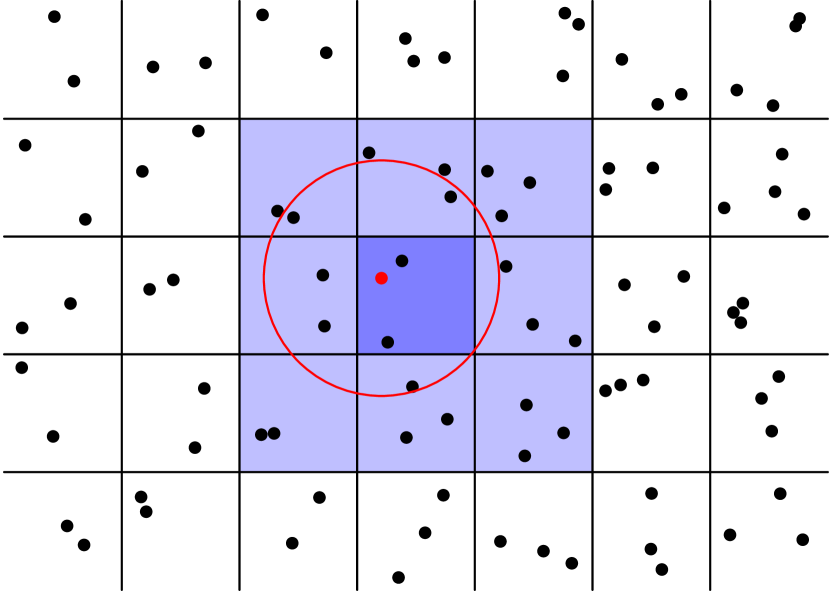
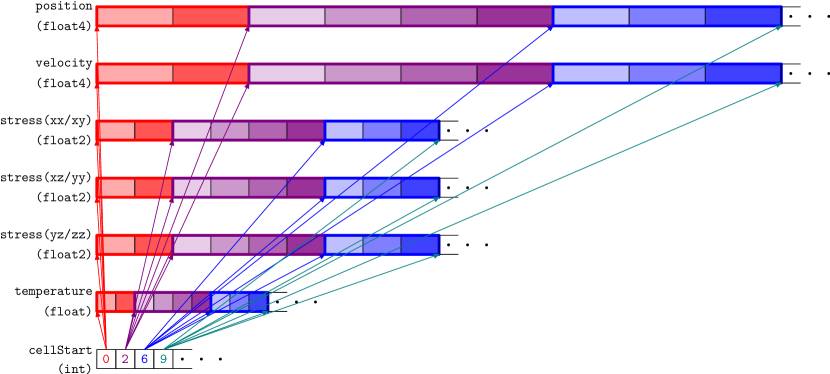
Figure 1: Grouping particles by reference cells with a cell-side which is not less that the neighbors search radius allows the search to be limited to the particles in the Moore neighborhood of the cell to which the central particle belongs (top). This requires a sorting process where the actual particle data is moved in memory so that the particles in the same cell are located next to each other. An additional array can be used to track the offset in memory where the data for the particles in each cell begins (bottom).

2.3 Optimizing the neighbors search

Each of the steps (with the possible exception of the integration steps) requires one or more loops (usually for summations) over the neighbors, pushing the need for an efficient neighbors search. The main strategy to improve the neighbors search performance is to adopt auxiliary data structures that help restrict the search space. Space partitions using trees are more common in applications where the smoothing length is variable: for example, $n$-trees (quadtrees in two dimensions, octrees in three) to bucket particles that are close in space are common in astrophysics, where they can be also used in support for gravity computation [29, 39]. A brief review of tree-based methods, with some proposed enhancements, can be found in [13].

A straightforward auxiliary data structure that is very practical in case of fixed smoothing lengths and that also has additional uses is a simple grid of cells with side length no less than the influence radius (Figure 1). The grid itself is represented simply by its origin (coordinates in 2D or 3D spaces), extents (dimensions in each coordinate direction), and grid spacing (which may be different in each coordinate direction). If particles are sorted in memory by the cell they belong to, bucketing can be achieved simply by storing the indices of the first and last particle in each cell. The particle sorting also brings performance benefits related to the improved data locality [32].

The primary objective of this auxiliary grid is to limit the neighbors search to the 9 (in 2D) or 27 (in 3D) cells around the central particle cell, but the same data structure is also useful to implement efficient multi-GPU and multi-node support [61, 60] and uniform accuracy in space without the need for extended precision [37, 63], by relying on local (cell-relative) particle positions.

Even with this improvements, the neighbors search can still be an expensive procedure, due also to the cost of maintaining the auxiliary data structures themselves, and/or to the particle sort. These costs however can be amortized (at the expense of memory consumption) by building a neighbors list per particle, to be rebuilt periodically [23]. The frequency at which the neighbors list needs to be rebuilt depends on the dynamics of the problem, and can be reduced by using a slightly larger radius for neighbors search compared to the actual influence radius. As we shall see in the upcoming sections, the way the neighbors list is stored, processed and built are essential details with a significant influence on the computational performance of an SPH implementation.

3 GPUSPH features

3.1 The SPH in GPUSPH

Born with the design goal of offering a simple, high-performance implementation of classic WCSPH [36], later extended with the aim to model lava flows [38, 7], GPUSPH has since grown into a very sophisticated engine for SPH, with the ultimate objective of becoming a universal SPH computational engine, useful both for applications and for research in the numerical method itself.

To improve its usability in the research of WCSPH, it is necessary for the GPUSPH code to be easily extensible, in order to minimize the cost of implementation of new formulations, and correct, in the sense of helping ensure that the operations are done in the intended order and on the intended data.

For applications, it is essential that the (correct!) results are provided in a timely manner, that they are stable (within the boundaries imposed by the model), and that invalid data is handled appropriately.

The priorities in GPUSPH development are therefore performance and robustness. Satisfying these goals concurrently poses a significant coding challenge, especially in consideration of the vastness of the problem.

The SPH core of GPUSPH is the so-called “simulation framework”, a collection of computational kernels specialized on the basis of user-selectable options that determine every aspect of the simulation: the equations to be solved (e.g. Navier–Stokes, heat, both), physical aspects such as the rheological or turbulence model, and choices about the details of the numerical model, such as the SPH formulation, the solid boundary model, the smoothing kernel, etc.

Dimensionality	1D, 2D, 3D
Smoothing kernel	Quadratic, Cubic spline,
	Wendland, Gaussian
SPH formulation	WCSPH single-fluid [50],
	WCSPH multi-fluid [18],
	Grenier [33], Hu & Adams [41]
Density diffusion	(none),
	Ferrari [28, 48], Brezzi [12, 26],
	Molteni & Colagrossi [49],
	Antuono ($\delta$-SPH) [46]
Boundary model	Lennard–Jones [44, 50], Monaghan–Kajtar [52],
	dynamic [21, 20], dummy [1],
	semi-analytical [27, 47]
Periodicity	(any combination of) X, Y, Z
Rheological models	Inviscid, Newton,
	Granular [30],
	Bingham [11], Papanastasiou [56],
	Power-law [55],
	Herschel–Bulkley [40], Alexandrou [3],
	DeKee & Turcotte [22], Zhu [77]
Turbulence model	(none),
	$k$-$\epsilon$ [25], Sub-Particle Scale (SPS) [59],
	artificial viscosity (improperly) [50]
Viscous model	Morris [53], Monaghan [50],
	Español & Revenga [24]
Averaging operator	arithmetic, harmonic, geometric
Internal viscosity	Dynamic
representation	Kinematic
Miscellanea	Adaptive time-stepping
(boolean flags)	XSPH
	Geometric planes support
	Geometric natural topography support
	Moving bodies support
	Open boundaries support
	Water depth computation
	Density summation
	Semi-analytical gamma quadrature
	Internal energy computation
	Multi-fluid support
	Repacking
	Implicit integration of the viscous term

Table 1: A summary of the framework options that can be set by the user when defining a test case in GPUSPH, with relevant bibliographical references. Not all combinations are supported. Some features are experimental and have not been fully merged into the public version yet.

The comprehensiveness of the framework can be remarked by looking at the variety of options offered, summarized in Table 1 for the latest publicly released version. The total number of possible theoretical combinations, considering all options, is between $10^{9}$ and $10^{10}$, and that’s before including additional options that have not been fully integrated in the public versions, such as coupling with the heat equation [7, 73], coupling with finite-element models [71], or kernel gradient corrections [75, 64]. Even though not all combinations are currently supported, the ultimate objective remains to cover the widest possible range. Still, to satisfy our goals of universality for both research and applications, this must be achieved without any performance penalty for unused options, and minimizing implementation complexity.

The lack of performance penalty for unused options is essential for the usefulness of GPUSPH in applications, and translates into the following maxim: the runtime of the program when a given framework option is not used/enabled should be the same as if support for that option had not been implemented in the code at all. This also means that when adding new features, there should be no regression in the runtime of any of the pre-existing options. This can be achieved by doing as much work as possible at compile time, and helping the compiler in producing optimal code by isolating code and variables that are specific to an option (see section 4 for details on how this is achieved).

3.2 Minimizing complexity

Figure 2: Call-tree for a subset of the functions involved in the computation of particle-particle interaction for the Navier–Stokes equation.

Minimizing implementation complexity, on the other hand, is a fight against Tesler’s law of conservation of complexity [62]. Our strategy is to maintain a high level of abstraction in the code, writing small functions and avoiding repetitions. This however comes at the cost of increased levels of indirection (Figure 2), a more spread-out code, and the adoption of non-trivial programming techniques centered around the C++ idiom known as template meta-programming, as described in Section 4.

Consider for example the case of the contribution of laminar viscosity to the momentum equation (central block in Figure 2). This can be expressed as

$$\phantom{K}\sum_{j}\omega_{ij}2\bar{\mu}_{ij}F_{ij}\mathbf{u}_{ij}$$

using Morris’ formulation [53], or as

$$K\sum_{j}\omega_{ij}2\bar{\mu}_{ij}F_{ij}\frac{\mathbf{x}_{ij}\cdot\mathbf{u}_{ij}}{\mathbf{x}_{ij}\cdot\mathbf{x}_{ij}}\mathbf{x}_{ij}$$

when using Monaghan’s [50], or in the form

$$\phantom{K}\sum_{j}\omega_{ij}F_{ij}\left(\left(\frac{5}{3}\bar{\mu}_{ij}-\bar{\zeta}_{ij}\right)\mathbf{u}_{ij}+5\left(\frac{1}{3}\bar{\mu}_{ij}+\bar{\zeta}_{ij}\right)\frac{\mathbf{x}_{ij}\cdot\mathbf{u}_{ij}}{\mathbf{x}_{ij}\cdot\mathbf{x}_{ij}}\mathbf{x}_{ij}\right)$$

following Español & Revenga [24]; in all these expressions, $\bar{\mu}_{ij}$ and $\bar{\zeta}_{ij}$ are some average first and second viscosity, and $\omega_{ij}$ is the volume-based neighbor weight.

The weight itself depends on the SPH formulation, being $\omega_{ij}=\frac{m_{j}}{\rho_{i}\rho_{j}}$ for most formulations, but e.g. $\omega_{ij}=\omega_{j}\left(\frac{1}{\sigma_{i}}+\frac{1}{\sigma_{j}}\right)$ when using Grenier’s formulation (see [33] for the meaning of $\sigma$). Likewise, the averaging operator can take many forms, including e.g. the specialized form in the case of harmonic mean of constant kinematic viscosity $\bar{\mu}_{ij}=2\nu\frac{\rho_{i}\rho_{j}}{\rho_{i}+\rho_{j}}$. Finally, when possible we also aim for simplifications across terms, so that for example $\omega_{ij}2\bar{\mu}_{ij}$ as a whole can be written as $4\nu\frac{m_{j}}{\rho_{i}+\rho_{j}}$ under appropriate conditions.

This leads to specializations with complex criteria such as single, Newtonian fluid when using kinematic internal viscosity representation with harmonic averaging, except when using Grenier’s formulation or the Español & Revenga viscous model.

Yield strength	Shear rate dependency
	Linear	Power-law	Exponential
none	Newton	Power-law
constant	Bingham	Herschel–Bulkley	DeKee & Turcotte
regularized	Papanastasiou	Alexandrou	Zhu
functional	Granular

Table 2: Decomposition of the contributions to the rheological models supported in GPUSPH. Separating each yield strength contribution and shear rate dependency in its own functions allow us to support 9 (potentially $4\times 3=12$) different models with only $4+3=7$ functions.

Finding the correct way to distribute the computations across multiple sub-functions helps reduce the complexity of the code. For example, a set of 4 functions for the yield strength contribution and 3 functions for the shear rate to shear stress contribution to the apparent viscosity of generalized Newtonian fluids is sufficient to describe 9 (potentially 12) different rheological models, as summarized in Table 2. By separating contributions and sharing common code, we reduce the number of necessary functions and follow the DRY (Don’t Repeat Yourself) principle.

3.3 Code structure

GPUSPH has four main components: the already-discussed simulation framework, the integrator, the manager and the worker(s).

Subclasses of the Integrator class describe the numerical integration scheme, as a sequence of phases (e.g. predictor, corrector), each composed of multiple steps or commands (e.g. apparent viscosity computation, forces computation, integration). This allows defining different integration schemes with limited or no need to change the other classes. GPUSPH currently implements only a predictor/corrector integration scheme, and an experimental explicit Euler used only for the repacking feature.

The manager (a class named GPUSPH) represents the main thread, and is responsible, as the name suggests, for managing the simulation, dispatching the commands (provided by the Integrator) to the workers or to secondary classes (such as the writers, responsible for saving the simulation results).

The workers are secondary threads that manage the device side of the simulation. One instance of the worker thread is created for each device (GPU), and it takes care of tasks such as memory allocation, cross-device data transfers, and issuing the actual computational kernels implementing the numerical method.

The computational kernels themselves are defined by the simulation framework, which is composed of distinct modules called “engines”, each dedicated to a separate aspect of the algorithm:

neibs engine

handles the construction of the neighbors list, including the reordering of the particle data so that particles close in space are also close in device memory (see Section 2.3);

visc engine

handles the computations related to non-Newtonian and turbulent viscous models;

boundary engine

handles the computations related to imposing boundary conditions;

forces engine

handles the computation of the “forces” of the particles, in the generalized sense of time derivatives of their state variables (including e.g. density and temperature);

euler engine

handles integration in time (despite the name of the engine, GPUSPH doesn’t actually use the forward Euler method directly, but an explicit predictor/corrector integration scheme, with a forthcoming option for a semi-implicit scheme [74, 8]).

Each engine is described by an abstract interface, and implemented by classes that specialize the interface based on the framework options. This allows the engine methods to be invoked by the workers with minimal knowledge about the framework options being used, delegating the gory details of the exact nature of the computations that need to be executed to the computational kernels defined by the specific engine incarnation.

This separation of roles is essential both for the multi-GPU and multi-node support in GPUSPH, and to reduce the complexity of implementation of new features: the latter effect is due to the reduction of the influence of the features onto each component to a “need-to-know” basis.

Listing 1: Subset of the AbstractForcesEngine definition, showing the interface for the forces engine used to compute particle dynamics.

⬇

class AbstractForcesEngine {

public:

/* omissis */

/// Compute density diffusion term

virtual void

compute_density_diffusion(

const BufferList& bufread,

BufferList& bufwrite,

const uint numParticles,

const uint particleRangeEnd,

const float deltap,

const float slength,

const float influenceRadius,

const float dt) = 0;

/* omissis */

}

Listing 2: Implementation of a command in the worker class, mapping the symbolic command name to the corresponding AbstractForces member function. Most command implementations follow the same structure.

⬇

template<>

void GPUWorker::runCommand<CALC_DENSITY_DIFFUSION>(CommandStruct const& cmd)

{

uint numPartsToElaborate = (cmd.only_internal ? m_particleRangeEnd : m_numParticles);

if (numPartsToElaborate == 0) return;

const int step = cmd.step.number;

const BufferList bufread = extractExistingBufferList(m_dBuffers, cmd.reads);

BufferList bufwrite = extractExistingBufferList(m_dBuffers, cmd.updates) |

extractGeneralBufferList(m_dBuffers, cmd.writes);

bufwrite.add_manipulator_on_write("calcDensityDiffusion" + to_string(step));

const float dt = cmd.dt(gdata);

forcesEngine->compute_density_diffusion(

bufread,

bufwrite,

m_numParticles,

numPartsToElaborate,

gdata->problem->m_deltap,

m_simparams->slength,

m_simparams->influenceRadius,

dt);

bufwrite.clear_pending_state();

}

Examples of the interfaces for the engines and how they are used by the workers are shown in Listings 1 and 2. The command implementation is nearly the same for most commands. The CommandStruct structure, defined by the integrator, holds metadata information about the command, such as which particle data should be made available to the engine function, how it should be accessed (for reading, for writing ignoring previous content, or for updating), and which value of the time-step should be used (depending on the integration step, this could be $\Delta t$ or $\Delta t/2$). This information is used by the worker function to extract the relevant subsets of the global list of particle data buffers, which are then passed to the engine function, together with the number of particles (total, and to be processed), geometric information such as the inter-particle spacing, smoothing length and influence radius, and the effective time-step being used. Additionally, buffers that will be written to by the engine function are marked with information that is useful when debugging, such as the commands and time-steps at which the buffer contents were modified.

Note that the worker function itself has no specific information about which buffers are going to be used for this specific command: this information defined on the integrator side, and then used on the engine side. This allows, for example, a new density diffusion formulation that uses different sets of particle data to be introduced by changing only the integrator and the engine, but not the worker, that is simply passing the information along.

3.4 The GPU in GPUSPH

GPUSPH was designed from the ground up to rely exclusively on GPUs for the computational part [36]. To achieve this, the program execution is split into three phases: initialization, simulation, and data storage.

The initialization phase runs on program startup, on the host CPU, and it takes care of generating the initial particle distribution, either from a geometric description of the domain or from data stored on disk (e.g. when resuming an interrupted simulation).

After initialization, the worker threads are created, instantiating a GPUWorker for each GPU selected for the simulation, and the domain particles are distributed to the GPUs (i.e. the first and last particle assigned to each GPU is computed). Each worker then allocates data arrays on its GPU, forming the global buffer lists, and the buffer contents are initialized by copying data over from the host, for the subset of particles assigned to the specific device.

These data arrays are the ones used by the computational kernels, extracted from the global buffer lists as shown in Listing 2, and passed to the appropriate engine functions, that take care of launching the actual computational kernels on the GPU.

No further data exchange between the GPU and the host happens, except for the following circumstances:

• after the particle sorting and neighbors list construction, the host fetches information about the current number of particles, and the maximum number of neighbors per particle; this information is used to check if particles have been removed because they had gone out of bounds, to track the new distribution of particles in multi-GPU when particles cross from one device to an adjacent one, and to check that all neighbors could be accounted for (issues with the number of neighbors typically indicate either an incorrect initial particle distribution, or some issues with the choice of formulation or its implementation);

• the maximum allowed time-step (minimum over all the particles) is computed on device using a parallel reduction, and then downloaded to the host, for time-keeping;

• for fluid/structure interaction, the cumulative forces and torques exerted by the fluid on each rigid body are computed on the GPU, and downloaded to the host, to be passed to Project Chrono to compute the motion of the rigid body; the updated position of the center of mass and rotation of the rigid bodies is then copied back to the GPU, where the information is used to move the body particles accordingly.

For multi-GPU (both single- and multi-node) simulations, data is transferred directly from device to device if possible, i.e. if the GPUs can access each other’s memory either through peering (on one machine) or through GPUDirect in multi-node configurations where the network setup supports it [60]. When this is not possible, data transfer happens through a staging area on host, which can negatively affect performance due to the additional memory copies.

Multi-GPU data transfers are explicitly marked by the integrator, allowing the developer to choose when to transfer data, and which data to transfer. These choices can be tuned to improve scaling by overlapping computations and data transfer [61, 60].

Finally, to allow data storage to disk, all particle data arrays get downloaded to the host at fixed (simulated) time interval selected by the user. The simulation is suspended during this process.

It should be noted also that the arrays are only allocated once during the initialization phase. If the number of particles decreases during the simulation, e.g. because some particles fly out of the computational domain, the contents of the arrays are compacted during sorting and the additional entries are simply ignored. Allocations are made taking into account the possibility of the number of particles increasing becase of open boundaries or in the multi-GPU case; in the open boundary case the user has control on the maximum number of particles that may be considered for the simulation, and in case of overflow the program terminates, allowing the user to resume with a higher upper bound. This avoids expensive reallocations at runtime.

4 C++11 and the benefits of template meta-programming

The abstract interfaces of the GPUSPH engines is preserved down the stack whenever possible. In particular, many computational kernels are as generic as possible as well, with the details further delegated to auxiliary functions, and so forth down to small, specialized functions that materialize one specific aspect of the computation, as exemplified in section 3.2. The key to writing such generic code in C++ is an extensive use of templates, combined with the coding strategies described in the following subsections, as illustrated in Listings 4 and 5 below.

A function template represents a family of functions that share a name, expose the same interface, and also frequently (but not necessarily) present the same body. Such a family of functions is parametrized through one or more template parameters, with each possible value (or combination of values) of these parameters ultimately dictating the actual function.

Template parameters are usually types, as in the classic examples of the std::min and std::max function templates from the C++ standard library, that allow the same function body (e.g. return a < b ? a : b) to be instantiated for each data type (int, float, double) without the known issues of the C preprocessor macros.

In GPUSPH however, most template parameters are enumeration types, such as the symbolic name of the SPH formulation or of the boundary conditions model. For example, the W and F function templates, used to compute the value of the smoothing kernel and the scalar part of its gradient, only depend on one template parameter, the KernelType enumeration value identifying the user choice of smoothing kernel. In this case, each specialization of the function templates W and F has a different body, since it must implement different computations (Listing 3).

Listing 3: Function templates for the smoothing kernel $W(\cdot,h)$ and its scaled gradient $F(\cdot,h)$. Some specialized instance are presented for demonstrative purposes. The normalization coefficients and the Gaussian truncation factor are device constants that are precomputed at the beginning of the simulation.

⬇

enum KernelType {

CUBICSPLINE, QUADRATIC, WENDLAND, GAUSSIAN,

};

template<KernelType kerneltype>

float W(const float r, const float slength);

template<KernelType kerneltype>

float F(const float r, const float slength);

// Wendland kernel: w(q) = (2q+1)(1 - q/2)^4, f(q) = (q-2)^3

template<>

float W<WENDLAND>(const float r, const float slength) {

const float R = r/slength;

float val = 1.0f - 0.5f*R;

val *= val; val *= val;

val *= 1.0f + 2.0f*R;

val *= d_wcoeff_wendland;

return val;

}

// Wendland kernel: f(q) = (q-2)^3

template<>

float F<WENDLAND>(const float r, const float slength)

{

const float qm2 = r/slength - 2.0f;

float val = qm2*qm2*qm2*d_fcoeff_wendland;

return val;

}

// d-truncated Gaussian kernel: w(q) = exp(-q^2) - exp(-(d/h)^2)

template<>

float

W<GAUSSIAN>(float r, float slength)

{

const float R = r/slength;

float val = expf(-R*R);

val -= d_wsub_gaussian;

val *= d_wcoeff_gaussian;

return val;

}

// Truncated Gaussian kernel: f(q) = -exp(-q^2)

template<>

float F<GAUSSIAN>(const float r, const float slength)

{

const float R = r/slength;

float val = -expf(-R*R)*d_fcoeff_gaussian;

return val;

}

/* and so on for the other smoothing kernels */

The advantage of function templates is that they eliminate a subset of the runtime conditionals, maximizing performance. For example, instead of checking which smoothing kernel was requested by the user every time W or F is evaluated, the selection is made once at compile time, eliminating conditionals from the hot path.

The downside is that the template parameters must be known at compile-time, since they are needed by the compiler to determine which versions of the function to emit, depending on what is being called. Because of this, template arguments “creep” up in the call chain up to the point where the user choice is given, affecting all functions and classes that directly or indirectly result in these functions being called. For example, any function (or computational kernel) that needs to call the W or F function templates will have to be a function template depending on the KernelType enumeration, and thus the framework engine classes that need to call these computational kernels will also have to be class templates that depend the same template parameter. Listings 4 and 5 show an example of this.

Listing 4: Declaration of the CUDAForcesEngine class template, concrete class implementing the AbstractForcesEngine interface, and example of a member function called by the appropriate GPUWorker::runCommand() specialization.

⬇

template<

KernelType kerneltype,

SPHFormulation sph_formulation,

DensityDiffusionType densitydiffusiontype,

typename ViscSpec,

BoundaryType boundarytype,

flag_t simflags>

class CUDAForcesEngine : public AbstractForcesEngine

{

/* omissis */

void

compute_density_diffusion(

BufferList const& bufread,

BufferList& bufwrite,

/* omissis */)

{

uint numThreads = BLOCK_SIZE_FORCES;

uint numBlocks = div_up(particleRangeEnd, numThreads);

auto params = density_diffusion_params<kerneltype, sph_formulation, densitydiffusiontype,

boundarytype, PT_FLUID>

(bufread, bufwrite, /* omissis */);

cuforces::computeDensityDiffusionDevice

<kerneltype, sph_formulation, densitydiffusiontype, boundarytype,

ViscSpec, simflags, PT_FLUID>

<<<numBlocks, numThreads>>>(params);

// check if last kernel invocation generated an error

KERNEL_CHECK_ERROR;

}

/* omissis */

};

Listing 5: Declaration of the computational kernel called by the corresponding member function of CUDAForcesEngine, implementing the actual computations, and its arguments structure template, leveraging conditional subclassing to determine which data members (i.e. function arguments) are present.

⬇

struct common_density_diffusion_params

{

float4 * __restrict__ forces;

const float4 * __restrict__ posArray;

const float4 * __restrict__ velArray;

/* omissis */

common_density_diffusion_params(

BufferList const& bufread,

BufferList & bufwrite,

/* omissis */)

:

forces(bufwrite.getData<BUFFER_FORCES>()),

posArray(bufread.getData<BUFFER_POS>()),

velArray(bufread.getData<BUFFER_VEL>()),

/* omissis */

{}

};

template<

KernelType _kerneltype,

SPHFormulation _sph_formulation,

DensityDiffusionType _densitydiffusiontype,

BoundaryType _boundarytype,

ParticleType _cptype>

struct density_diffusion_params :

common_density_diffusion_params,

cond_struct<_boundarytype == SA_BOUNDARY, sa_boundary_params>

{

/* omissis */

density_diffusion_params(

BufferList const& bufread,

BufferList & bufwrite,

/* omissis */)

:

common_density_diffusion_params(bufread, bufwrite, /* omissis */),

cond_struct<_boundarytype == SA_BOUNDARY, sa_boundary_params>(bufread)

{}

};

template<KernelType kerneltype,

SPHFormulation sph_formulation,

DensityDiffusionType densitydiffusiontype,

BoundaryType boundarytype,

typename ViscSpec,

flag_t simflags,

ParticleType cptype>

__global__ void

computeDensityDiffusionDevice(density_diffusion_params<kerneltype, sph_formulation,

densitydiffusiontype, boundarytype, cptype> params)

{

// Global particle index

const uint index = INTMUL(blockIdx.x,blockDim.x) + threadIdx.x;

if (index >= params.particleRangeEnd) return;

/* omissis: actual computation of the density diffusion contribution */

}

A class template represents a family of classes that expose the same (or similar) interfaces, member variables and member functions (methods). Classic examples in the C++ standard library are the container classes such as std::vector or std::map. In GPUSPH, class templates are used extensively in the host code to represent things such as buffers, integrator schemes, the simulation framework and its engines, and in device code for the variables and arguments structures that will be discussed in the following sections.

A powerful use of class or structure templates in C++ is the traits concept: these are structure templates that hold a collection of properties associated with specific values of its template parameters. In the standard library, for example, the representation limits of each data type (minimum and maximum representable value, number of digits etc) are collected into the std::numeric_limits structure template (rather than in preprocessor macros as in the C standard).

One of the primary uses of type traits in GPUSPH is the BufferTraits structure template, that associates the symbolic name of each buffer with the type of the elements, the number of arrays associated with the buffer, and a user-readable name. For example, the traits declare BUFFER_POS to be a single array of float4 elements, named “Position”, while BUFFER_TAU is a triple array of float2 elements (needed to store the 6 elements of a symmetric tensor) named “Tau”. This information allows GPUSPH to do type-checking on the buffers when they get passed to computational kernels, and to support most memory management and data exchange (between host and devices on initialization and when saving data, or between devices in multi-GPU and multi-node setups) automatically through common interfaces.

Type traits are just one of the keys to template meta-programming [2], a C++ coding strategy that improves code abstraction and minimization. With version 5 of GPUSPH, and the drop of support for older version of CUDA that had so far prevented us from adopting more recent versions of the C++ standard, we have finally transitioned to C++11 [66] as the minimum C++ version for both the host and the device code. This has allowed us to leverage the facilities offered by the new language revision to improve the compactness and legibility (and sometimes the expressive power) of our templates.

We will discuss here three meta-programming techniques heavily used in the device code of GPUSPH, to show how they allow us to minimize repetition (DRY principle) while also reducing the compiler-visible variables and function arguments to the minimum necessary for each specialization of a computational kernel or function. All of these features can be implemented without relying on C++11 features, but the syntax on older revisions of the C++ language is considerably more convoluted to use. Much of the syntax could be further simplified by raising the minimum requirements of more recent versions of CUDA that support C++14, but we chose to compromise to extend the range of hardware supported by GPUSPH, since newer CUDA versions tend to deprecate support for older hardware.

4.1 Conditional structures

One of the main complexities associated with supporting different physical-numerical models is that each of them will require keeping track of different state variables for the particles, and will need different function arguments to be passed to the computational kernels and their auxiliary functions.

For example, when using the $k$-$\epsilon$ turbulence model [25] one will need to track $k,\epsilon$ and their derivatives, whereas these properties (and all the associated computations) will not be needed when using a different (or no) turbulence model. Likewise, when using the “dummy boundary” [1] model, boundary particles will have an associated “viscous velocity” used when computing the viscous term in the momentum equation for neighboring fluid particles, but the particle velocity alone may suffice for all other particles and/or other boundary models.

To help the compiler produce optimal code, and to avoid unintended mangling due to developer error, we wish the corresponding variables and function arguments to not be present in the computational kernel specializations that do not need them.

Focusing on variables (the discussion is exactly the same for arguments), the basic idea is that, instead of declaring each variable independently, we define a structure whose members correspond to the original variables. This transforms the problem of not having unnecessary variables to the problem of not having unnecessary members in the structure.

The transformed problem can be solved using the conditional inheritance paradigm, i.e. the possibility to have a class templates declare different base classes depending on the template parameters. The idea is to collect optional members (variables) into their own structures, and then have the full structure derive only from the substructures that are required by the specific combination of framework options. This can be achieved using the std::conditional structure template provided from C++11 onwards, which is defined in such a way that

will be equivalent to TrueClass if the boolean value b is true, and to FalseClass if it’s false. On older revisions of C++, the same structure template can be defined by the user in the following way:

⬇

struct conditional { typedef T type; };

template<typename T, typename F>

struct conditional<false, T, F> { typedef F type; };

although some of the syntax simplifications illustrated later on will not be possible.

By making the FalseClass an empty structure, we can achieve our goal of selective inclusion of member variables. Given for example the structure template presented in Listing 6, the all_variables<DUMMY_BOUNDARY> specialization would have members dummy_vel, pos and vel, whereas a specialization for a different BoundaryType (e.g. all_variables<DYN_BOUNDARY>) would only have pos and vel, since the base structure would be the memberless empty structure in this case.

Listing 6: Simple application of conditional inheritance. The all_variables structure template will only have the dummy_vel member in the all_variables<DUMMY_BOUNDARY> specialization.

⬇

struct empty {};

struct dummy_boundary_variables {

float3 dummy_vel;

};

template<BoundaryType boundarytype>

struct all_variables :

std::conditional<boundarytype == DUMMY_BOUNDARY,

dummy_boundary_variables, empty>::type

{

float3 pos;

float3 vel;

};

There are two issues with this naive approach: one is that we cannot have multiple independent conditional base structures, and the other is related to constructors for the optional classes.

For the case of multiple optional components, consider the example in Listing 7 where we have added an additional optional structure holding the variables for the $k$-$\epsilon$ turbulence model. Now, when neither of the optional base structures are needed (e.g. for an all_variables<DYN_BOUNDARY, SPS> combination), the specialization of all_variables would have the empty structure as base class twice, which is not allowed in C++.

Listing 7: Non-working example of conditional inheritance with multiple optional components.

⬇

struct empty {};

struct dummy_boundary_variables {

float3 dummy_vel;

};

struct ke_variables {

float turb_k;

float turb_eps;

};

template<BoundaryType boundarytype, TurbulenceModel turbmodel>

struct all_variables :

std::conditional<boundarytype == DUMMY_BOUNDARY,

dummy_boundary_variables, empty>::type

std::conditional<turbmodel == KEPSILON,

ke_variables, empty>::type

{

float3 pos;

float3 vel;

};

The solution is to turn empty itself in a structure template, whose argument is the class that is going to be replaced: this will make each specialization formally unique (Listing 8), although it makes the syntax considerably heavier.

Listing 8: Working example of conditional inheritance with multiple optional components.

⬇

template<typename T>

struct empty {};

struct dummy_boundary_variables {

float3 dummy_vel;

};

struct ke_variables {

float turb_k;

float turb_eps;

};

template<BoundaryType boundarytype, TurbulenceModel turbmodel>

struct all_variables :

std::conditional<boundarytype == DUMMY_BOUNDARY,

dummy_boundary_variables,

empty<dummy_boundary_variables> >::type,

std::conditional<turbmodel == KEPSILON,

ke_variables, empty<ke_variables> >::type

{

float3 pos;

float3 vel;

};

With C++11, the syntax can be simplified by using type alias templates like in Listing 9, whereas with older C++ versions a less robust preprocessor macro can be used for the same effect.

Listing 9: Type alias templates to simplify the optional base class syntax.

⬇

template<bool B, typename T>

using cond_struct = typename std::conditional<B, T, empty<T>>::type;

template<BoundaryType boundarytype, TurbulenceModel turbmodel>

struct all_variables :

cond_struct<boundarytype == DUMMY_BOUNDARY,

dummy_boundary_variables>,

cond_struct<turbmodel == KEPSILON, ke_variables>

{

float3 pos;

float3 vel;

};

The remaining issue pertains the construction of the base classes. We would like a syntax such as the one in Listing 10 to work for both the true and false cases, but this requires the empty template to accept the same arguments as the structures it replaces, which may be varied in number and type.

Listing 10: Constructing the variables structure from the constructors of the optional base classes.

⬇

template<BoundaryType boundarytype, TurbulenceModel turbmodel>

struct all_variables :

cond_struct<boundarytype == DUMMY_BOUNDARY,

dummy_boundary_variables>,

cond_struct<turbmodel == KEPSILON, ke_variables>

{

float3 pos;

float3 vel;

all_variables(/* arguments used to construct all members,

including the optional ones */)

:

cond_struct<boundarytype == DUMMY_BOUNDARY,

dummy_boundary_variables>

(/* arguments to construct dummy_boundary_variables */),

cond_struct<turbmodel == KEPSILON, ke_variables>

(/* arguments to construct ke_variables */),

pos(/* arguments to construct pos */),

vel(/* arguments to construct vel */)

{}

};

The solution is to provide the empty template with a generic constructor that can take any argument (and ignore it). This could be simply a variadic constructor empty(…) {}, but this is not supported in CUDA code by some compiler version, even when the effect of the constructor is trivial like in the case of the empty template.

The alternative, assuming C++11 support, is to use variadic templates for the same purpose (the universal constructor in Listing 11). With older C++ revisions, the only solution is to provide one template constructor for each given number of arguments, as shown in Listing 11 for the alternative preprocessor branch.

Listing 11: The full empty template, with constructors.

⬇

template<typename>

struct empty

{

// Empty constructor

empty() {}

#if __cplusplus >= 201103L

// C++11 and higher: universal empty constructor

template<typename ...T1>

empty(T1 const&...) {}

#esle // __cplusplus < 201103L

// Before C++11: one constructor per number of arguments

template<typename T1>

empty(T1 const&) {}

template<typename T1, typename T2>

empty(T1 const&, T2 const&) {}

template<typename T1, typename T2, typename T3>

empty(T1 const&, T2 const&, T3 const&) {}

// .., and so on as needed

#endif

};

In GPUSPH, this technique was first used for the forces computational kernel, which is the most complex and computationally intensive kernel, for which we defined a forces_params structure template to collect all the arguments (mostly: arrays of particle data) to be passed to the forces specializations, and for the variables structures, collected by use: particle_data to collect the properties of the current particle, neib_data to collect the properties of the current neighbor, neib_output to collect the contributions from the current neighbor, and particle_output to gather all of the contributions affecting the evolution of the current particle (Listing 12).

Listing 12: The declarations of the parameters structure and variables structures used by the forces computation kernel.

⬇

template<KernelType kerneltype,

SPHFormulation sph_formulation,

BoundaryType boundarytype,

ViscosityType visctype,

flag_t simflags>

struct forces_params;

template<KernelType kerneltype,

SPHFormulation sph_formulation,

BoundaryType boundarytype,

ViscosityType visctype,

flag_t simflags>

struct particle_data;

template<KernelType kerneltype,

SPHFormulation sph_formulation,

BoundaryType boundarytype,

ViscosityType visctype,

flag_t simflags>

struct neib_data;

template<KernelType kerneltype,

SPHFormulation sph_formulation,

BoundaryType boundarytype,

ViscosityType visctype,

flag_t simflags>

struct neib_output;

template<KernelType kerneltype,

SPHFormulation sph_formulation,

BoundaryType boundarytype,

ViscosityType visctype,

flag_t simflags>

struct particle_output;

Historical note: adopting this strategy in GPUSPH did not produce any performance benefit, since it replaced an ad-hoc solution where a similar effect was obtained through an approach where the same “model” body of the kernel was defined in its own file that was included multiple times, each with a different set of defines that would identify the specific variant of the kernel to be built, and using conditional preprocessing to exclude unnecessary variables, following what is known as the X-Macro technique. This strategy was actually imposed on us by limitations in the number of template parameters in first versions of the CUDA compilers.

Even without performance benefits, conditional inheritance still presents significant advantages compared to the X-Macro approach, particularly in terms of source code simplification, higher readability with no preprocessor conditionals, and most importantly a significantly reduced developer burden when adding new features, and particularly new template parameters. The latter benefit was additionally boosted by its combination with the thorough refactoring allowed by the specialization based on the SFINAE (Specialization Failure Is Not An Error) principle, that will be described further on (section 4.3).

4.2 Reducing the number of template arguments

The extensive use of arguments and variables structures propagates to all auxiliary function templates. In fact, most if not all variables structures in the computational kernels (or rather kernel templates) are effectively also the arguments structures of the auxiliary functions (or rather function templates) called by the kernel. This can cause an increase in the maintenance burden.

Indeed, as the number of framework options grows, so does the list of template arguments to computational kernel templates and their arguments and variables structure templates, as well as to the auxiliary function templates to which the computations are delegated. This inflicts a high development cost, since the introduction of a new set of framework options requires changing the list of template parameters of most functions, even when many of them may not be actually affected by the new parameter (in the sense that its value wouldn’t alter the function definition or behavior), and the only reason why the function needs to have the template parameter is to be able to define the type of its arguments structure.

Listing 13: Propagating individual framework options as template arguments.

⬇

template<KernelType kerneltype,

SPHFormulation sph_formulation,

BoundaryType boundarytype,

ViscosityType visctype,

flag_t simflags>

void particleParticleInteraction(

particle_data<kerneltype, boundarytype, visctype, simflags>

const& pdata,

neib_data<kerneltype, boundarytype, visctype, simflags>

const& ndata,

neib_output<kerneltype, boundarytype, visctype, simflags>&

nout,

particle_output<kerneltype, boundarytype, visctype, simflags>&

pout)

{ /* omissis: compute particle-particle interaction */ }

template<KernelType kerneltype,

SPHFormulation sph_formulation,

BoundaryType boundarytype,

ViscosityType visctype,

flag_t simflags>

void forces(

forces_params<kerneltype, boundarytype, visctype, simflags> params)

{

particle_data<kerneltype, boundarytype, visctype, simflags>

pdata( /* omissis: initialize particle data */ )

particle_output<kerneltype, boundarytype, visctype, simflags>

pout;

for_each_neighbor( /* omissis */ ) {

neib_data<kerneltype, boundarytype, visctype, simflags>

ndata( /* omissis: initialize particle data */ )

neib_output<kerneltype, boundarytype, visctype, simflags>

nout;

particleParticleInteraction(pdata, ndata, nout, pout);

}

/* omissis */

}

This is illustrated in Listing 13: adding a new framework option (e.g. to enable support for the heat equation) would require it to be included not only in the definition of all the arguments and variables structures seen in Listing 12, that would need it to determine which new members to include through the technique described in Section 4.1, but also in the declaration of forces, particleParticleInteraction and any functions called by them and taking those same structures as input.

The solution we have adopted in GPUSPH is to use a single template parameter for each argument: the unspecified type of the argument itself. Referring to the same example in Listing 13, the singatures for forces and particleParticleInteraction would simplify to

⬇

template<typename P, typename N, typename NO, typename PO)

void particleParticleInteraction

(P const& pdata, N const& ndata, NO& nout, PO& pout);

where FP is assumed to be some specialization of the forces_params arguments structure template, and the typenames P, N, NO, PO are assume to stand for some specialization of particle_data, neib_data, neib_output and particle_output respectively.

When the body of the function template doesn’t depend on the specific specialization of the parameter structure template, this allows us to pass on the differentiation down to any called function that needs it When differentiation is wanted, it will be necessary to access the original template parameters (i.e. the values of the framework options): e.g. we might want to know which specific value of BoundaryType was used to specialize the forces_params structure that is passed to the kernel. C++ does not provide such a feature, but it can be achieved by adding appropriate static members to the structure template: a static constexpr member for each value type template parameter, and a type alias for each typename template parameter (constexpr, introduced in C++11, can be replaced with a simple const on older revisions of C++).

Listing 14: Static constant members can be used to expose the template parameters used to specialize the structure.

⬇

template<KernelType kerneltype_,

SPHFormulation sph_formulation_,

BoundaryType boundarytype_,

ViscosityType visctype_,

flag_t simflags_>

struct forces_params /* omissis: conditional base classes */

{

static constexpr KernelType kerneltype = kerneltype_;

static constexpr SPHFormulation sph_formulation =

sph_formulation_;

static constexpr BoundaryType boundarytype =

boundarytype_;

static constexpr ViscosityType visctype = visctype_;

static constexpr flag_t simflags = simflags_;

/* omissis: constructors etc */

};

template<typename P, /* specialization of particle_data */

typename N, /* specialization of neib_data */

typename NO, /* specialization of neib_output */

typename PO> /* specialization of particle_output */

void particleParticleInteraction(Pt const& pdata, Nt const& ndata,

NO& nout, PO& pout)

{ /* omissis: compute particle-particle interaction */ }

template<FP /* specialization of forces_params */>

void forces(FP const& params)

{

particle_data<FP::kerneltype, FP::boundarytype,

FP::visctype, FP::simflags> pdata

( /* omissis: initialize particle data */ )

particle_output<FP::kerneltype, FP::boundarytype,

FP::visctype, FP::simflags> pout;

for_each_neighbor( /* omissis */ ) {

neib_data<FP::kerneltype, FP::boundarytype,

FP::visctype, FP::simflags> ndata

( /* omissis: initialize particle data */ )

neib_output<FP::kerneltype, FP::boundarytype,

FP::visctype, FP::simflags> nout;

particleParticleInteraction(pdata, ndata, nout, pout);

}

/* omissis */

}

This is illustrated in Listing 14, where the specific values for the kernel type, boundary model, etc used to defined the specialization of forces_params that will be passed to forces are accessible within the function itself through FP::kerneltype, FP::boundarytype, etc. Moreover, this information will be available at compile time, exactly as if it had been specified as a template parameter to the function itself, and can thus be used e.g. in the specification of additional dependent types or auxiliary functions, which is used in Listing 14 to specify the template arguments of the pdata, ndata, nout and pout variables structures that will be passed to particleParticleInteraction.

The most valuable upside to this single-parameter approach to function templates is its simplicity, without any loss of expressive power. This comes at the cost of reduced type checking. It would indeed be possible to pass anything to the function templates mention before, even something that is not a specialization of the expected template (e.g. something that is not a forces_params specialization for forces in Listing 14).

This is however for the most part only a theoretical issue, as in most cases the instantiation of the template or of any of the auxiliary functions will trigger a compilation error when trying to access a non-existent member for anything but a specialization of the correct structure. Moreover, the possibility to plug in almost arbitrary data structures for these generically-specified arguments structures actually gives more flexibility, since it allows the same function templates to be used with potentially unrelated structures that still present the same (or similar) sets of member variables, thereby improving the genericity of the code by supporting a form of duck typing. This is actually a benefit, especially for the smaller functions down the call chain that may get passed variables structures from different computational kernels.

For example, some density diffusion contributions may be computed during the forces computation (thus receiving the variables structures from the forces kernel) or as a separate post-integration step (thus receiving the variables structures from a dedicated densityDiffusion kernel), depending on the scheme being employed. Duck typing allows the same device function to compute the contribution in both cases, provided the members of the variables structures have the same name and meaning.

In fact, the only practical downside we have found to this approach has been, as developers, the sometimes overwhelming complexity of the error messages when the instantiation of a specialized version of a structure or function template fails. Template errors in C++ are notoriously long-winded and hard to decipher, to the point of being commonly classified as horrific. This issue is compounded, in CUDA, by a paradoxical lack of useful information from the nvcc compiler in some instances (particularly in combination with the SFINAE tricks we will discuss momentarily), a fact that was actually one of the driving forces for exploring alternative compilers, with the surprising results discussed in section 8.

4.3 SFINAE for function template specialization

The remaining C++ programming feature employed in our effort to improve the genericity of the code pertains the specialization of function templates with several template parameters, but for which the specialization depends on a single parameter.

Assume for example we have a function template f depending on the boundary type and turbulence model, for which we would like to write a specialization for the case of the $k$-$\epsilon$ turbulence model, regardless of the boundayr type. Since C++ does not support partial function template specialization, something like

⬇

template<BoundaryType boundarytype> void f<boundarytype, KEPSILON>

( /* omissis */ )

would be invalid syntax.

The idiomatic way to achieve the intended effect (that we have extensively adopted in GPUSPH version 5) relies on the C++ feature known as Specialization Failure Is Not An Error (SFINAE). According to the language specification, when trying to resolve a function name, any function template for which template parameter deduction would result in an error is simply ignored. This allows a form of partial specialization to be achieved by overloading the function template, but allowing one, and only one overload to resolve correctly based on the intended specialization.

The fundamental building block for this is a structure template that declares the actual return type of the function template in the positive case, but does not declare anything as return type (and thus results in an error, and the discard of the overload) otherwise.

In C++11, this type is provided by the standard library std::enable_if, a structure template such that std::enable_if<true, T>::type will resolve to the type name T, whereas std::enable_if<false, T>::type will result in an error (the type name T can actually be omitted, in which case void is assumed by default). A similar structure can be defined by hand also in earlier revisions of the C++ language:

⬇

struct enable_if {}; /* no ‘type‘ member, to cause an error */

template<typename T>

struct enable_if<true, T> { typedef T type; };

but C++11 brings with itself not only the definition out of the box, but also the possibility to define a type alias template to simplify syntax:

⬇

using enable_if_t = typename enable_if<B, T>::type;

so that enable_if_t<bool, T> can be used as a shorter form for enable_if<bool, T>::type. This type alias template is predefined since C++14.

Partial specialization can then be achieved by defining multiple overloads of the function templates, with a return type in the form enable_if_t<condition, actual_return_type>, and using mutually exclusive conditions for each of the partial spcializations. For example, assuming that void is the return type of our f function template above, we can use:

⬇

enable_if_t<turbmodel == KEPSVISC> f(...)

{ /* code for the KEPSVISC case */ }

template<BoundaryType boundarytype, TurbulenceModel turbmodel>

enable_if_t<turbmodel != KEPSVISC> f(...)

{ /* code for the non-KEPSVISC cases */ }

to fulfill our need to specialize f for the $k$-$\epsilon$ turbulence model.

This feature can be combined very efficiently with the template argument reduction discussed in section 4.2:

⬇

enable_if_t<AV::turbmodel == KEPSVISC> f(AV& args)

{ /* code for the KEPSVISC case */ }

template<typename AV>

enable_if_t<AV::turbmodel != KEPSVISC> f(AV& args)

{ /* code for the other cases */ }

with the added benefit of causing a compiler error if an incompatible argument type (specifically, one without a turbmodel static constant member) is passed to f, since the compiler will discard both specializations (with the SFINAE-ignored failure being the inability to access turbmodel) and complain about being unable to resolve the function name.

5 Putting it all together: split neighbors

The adoption of the meta-programming techniques discussed so far has been the key to one of the most significant performance boost from version 4 to version 5 of GPUSPH: the split neighbors list processing, which has brought a typical performance improvement between 15% and 30%, depending on the combination of framework options and hardware capabilities [10, 9].

Analysis of the performance of the forces computational kernel in version 4 revealed that, despite the high density of computational operations in the kernel, its runtime was still largely memory-bound. The main cause for this was tracked down to the large number of variables that had to be allocated during the processing of the particle-particle interactions, which resulted in them overflowing the register banks of the GPU multiprocessors, resulting in the usage of the much slower VRAM as temporary storage (termed local memory in CUDA).

This large register pressure was ascribed to the monolithic nature of the kernel and the disparity of behavior in the interaction between particles of different types: indeed, for most boundary models fluid-fluid particle interactions are different from fluid-boundary particle interactions, but since particles are stored all together, and the neighbors list stored all neighbors together (without distinction of type), during execution of the monolithic kernel each work-item would load the data for the particle being processed, and then traverse the entire neighbors list, deciding at runtime how to interact with each specific neighbor, based on the neighbor type.

This led to a growth in the register usage, since the total number of variables that needed to be allocated was no less than the union of the variables needed for each of the particle-particle interaction types. This approach also led to additional performance loss due to the runtime decision about the kind of interaction, and the possible divergence of execution code-paths due to disparity of interaction between pairs of particles being processed concurrently, a well-known performance issue on GPUs.

Listing 15: Full template signature for the forces computational kernel as of version 5 of GPUSPH, showing also the use of optional template arguments as a shortcut to expose the static constant members of the arguments structure template forces_params (in order to make them accessible within the function body without the FP:: prefix), and the addition of the central (cptype) and neighbor (nptype) particle type as template parameters (in forces_params and inherited in forces) for the split-neighbors implementation.

⬇

template<typename FP, /* forces_params<kerneltype, sph_formulation, etc> */

KernelType kerneltype = FP::kerneltype,

SPHFormulation sph_formulation = FP::sph_formulation,

DensityDiffusionType densitydiffusiontype = FP::densitydiffusiontype,

BoundaryType boundarytype = FP::boundarytype,

typename ViscSpec = typename FP::ViscSpec,

flag_t simflags = FP::simflags,

ParticleType cptype = FP::cptype,

ParticleType nptype = FP::nptype>

void forcesDevice(FP params)

The solution we adopted has been to split the forces kernel into a separate specialization for each of the particle-particle interaction pairs: one for fluid to fluid, one for fluid to boundary, one for boundary to fluid, etc. Hence, the forces_params parameters structure template and all the variables structure templates for the forces computational kernel depend not only on the framework parameters, but also on the central and neighbor particle type, as illustrated in Listing 15 that shows the declaration of the function as of versio 5 of GPUSPH.

The split has been particularly meaningful for the semi-analytical boundary conditions [27, 47], that have three different particle types, larger disparities in the treatment of different pairs, and complex rules to decide which pairs should be computed: even just moving most of the decision logic outside of the device-side computational kernel to the host-side has given a measurable performance gain of a few percents.

Reducing the complexity of the logic inside each instance of the computational kernel (now one per pairwise combination of particle types) gives more optimization opportunities to the compiler, especially when most of the conditions end up depending only on template parameters, whose value is known at compile time. On the other hand, by itself this strategy is insufficient, since leaving the kernel body and associated data structures unchanged leaves two main reasons of inefficiency.

The first comes from the need to issue each specialization of the kernel on the entire set of particles, with each specialization then skipping the particles whose type is different from the requested one. For example, the fluid-fluid and fluid-boundary versions would skip non-fluid particles. This can be solved by creating a separate particle system for each particle type, and issuing each version of the kernel only on the particle system of the correct type. However, since fluid particles are generally an order of magnitude more than the other particle types, the impact of the loss is relatively low, while the implementation cost of the solution is quite high, so that optimizing this aspect has been considered “second-order”, and therefore postponed.

The second inefficiency comes from the traversal of the neighbors list: when all neighbors are stored together, regardless of type, it will be necessary to randomly skip elements from the neighbors list during its traversal. This can be quite costly, as it is again a likely source of divergence at the hardware level. We have solved the issue by redesigning the way neighbors are stored in the list, in such a way that all neighbors of the same type are stored consecutively, while preserving GPU-optimal access patterns and without increasing the storage requirements.

5.1 Efficient split neighbors list

Memory access is a significant bottleneck on most modern computational hardware, be it CPUs or GPUs. This is the main reason for the growing, multi-layer caches of CPUs, and the introduction of L1 and L2 caches even on GPUs. Optimal memory access patterns can significantly speed up an implementation, but the optimality of the patterns depends not only on the nature of the algorithm, but also on the characteristics of the hardware.

On a mostly sequential processor like a CPU, the best cache usage is obtained by placing the data needed by a single thread in adjacent memory locations. By contrast, on stream processing hardware like GPUs, optimal access patterns require that adjacent memory locations refer to data needed concurrently by different work-items.

Let us consider the case of the neighbors list, and let us denote by $n_{i}(j)$ the index of the $i$-th neighbor of the $j$-th particle. When traversing the neighbors list, a thread or work-item processing particle $j$ will need to read the index of the first neighbor ($n_{0}(j)$), then the index of the second neighbor ($n_{1}(j)$), and so on.

For sequential hardware (such as CPUs), it is then optimal to lay out the neighbors indices in memory grouping them by particle:

$$n_{0}(0),n_{1}(0),\dots,n_{k}(0),n_{0}(1),n_{1}(1),\dots,n_{k}(1),\dots$$

where $k+1$ is the maximum number of neighbors per particle. This will ensure that whenever a neighbor index is loaded from memory, the following neighbors indices will be cached too.

(Note: for efficiency reason, we use a fixed-size neighbors list, so that the neighbors of each particle can be found by simple computations, without additional memory accesses. A special marker is added to the list of neighbors of each particle if it’s not full, to indicate the actual end.)

By contrast, on GPUs we want to lay out the list in memory in such a way that when work-items $j,j+1,\dots$ load the index of their respective first neighbor from memory, they will find it in adjacent memory locations. In this case it is therefore optimal to lay out the neighbors indices in memory grouping them by ordinal:

$$n_{0}(0),n_{0}(1),\dots,n_{0}(p),n_{1}(0),n_{1}(1),\dots,n_{1}(p),\dots$$

where $p$ is the number of particles.

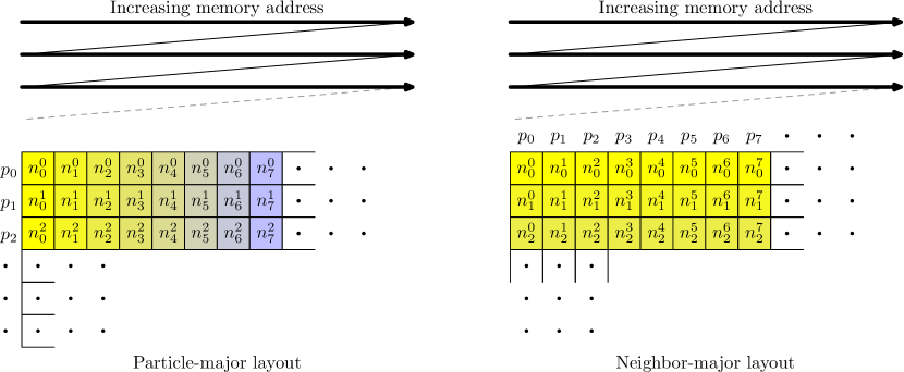
Figure 3: Different layouts for the neighbors list, comparing the CPU-preferrable “by particle” to the GPU-preferrable “by neighbor” order.

We call this layout interleaved or neighbor-major, in contrast to the sequential or particle-major layout used for CPUs, since from the perspective of each particle, the next neighbor is not found with an offset $+1$, but with an offset $+p$, with the memory in-between dedicated to the same neighbor ordinal for the other particles (Figure 3).

This works very well when the entire neighbors list must be traversed each time, but is sub-optimal when we want to only traverse a subset of the list (for example, as we do in GPUSPH, considering only the neighbors of a given type).

To illustrate the approach we adopted, assume at first that we have only two particle types (fluid and boundary), and that when there are more neighbors of one type, there will be fewer of the other type. This is consistent with the fact that a particle far from the boundary will have a full neighborhood of fluid particles, but as it gets closer to the boundary the number of fluid neighbors will decrease, while the number of boundary neighbors will increase at a similar rate (assuming a more-or-less uniform particle distribution).

The solution to the split neighbors list in this case is to collect all neighbors of one type at the beginning of the list (from the first location up), and all the neighbors of the other type at the end of the list (from the last location down). If we denote by $f_{i}$ the $i$-th fluid neighbor and $b_{i}$ the $i$-th boundary neighbor, from the perspective of a single particle, the neighbors would then be stored as:

$$f_{0},f_{1},f_{2},\dots,f_{k_{f}},\odot,\dots,\odot,b_{k_{b}},\dots,b_{2},b_{1},b_{0}$$

where $k_{f}+1$ is the number of fluid neighbors, $k_{b}+1$ the number of boundary neigbors, and $\odot$ denotes the end-of-list marker. Of course this single-particle perspective can then be implemented system-wide using either the sequential layout, or with the interleaved layout.

Figure 4: Split-neighbors-list layout in the neighbor-major order case.

The situation is more complex when the number of particle types grows. In the case of a third type, for example (as is the case for the semi-analytical boundary conditions with their vertex particles), the neighbors list will need to be split into two fixed-size chunks, one to store the first pair of types, and the other to store the remaining type (Figure 4); indicating as before with $f_{i},b_{i},v_{i}$ respectively the $i$-th fluid, boundary and vertex neighbor, and with $k_{v}$ the number of vertex neighbors, the list as seen by each particle would be coded as:

$$f_{0},f_{1},f_{2},\dots,f_{k_{f}},\odot,\dots,\odot,b_{k_{b}},\dots,b_{2},b_{1},b_{0},v_{0},v_{1},v_{2},\dots.v_{k_{v}}\odot$$

In this case, it’s necessary to know the size of the chunk. In GPUSPH, we store the (local) index of the first boundary neighbors index, knowing that the vertex neighbors will start at the next location.

6 Textures versus linear memory

One of the key differences between GPUs and CPUs is the possibility to access global memory not only through the standard linear addressing mode, but also through the texture mapping units (TMUs), dedicated hardware that supports a number of features such as multi-dimensional addressing, hardware interpolation and type conversion (e.g. from integer type to normalized floating-point values).

On older GPU architectures, using textures was also the only way to have some kind of caching, due to the TMU approach of loading a small neighborhood of the pixel values when fetching the data for a single pixel.

Judicious use of textures and linear memory addressing has thus been a sure-fire way in GPUSPH to maximize memory throughput, even after the introduction of the L1 and L2 caches in more modern GPU architectures, at least until the introduction of a unified texture and L1 cache in the Pascal architecture.

Since linear and texture memory addressing requires different function calls, and the distribution of the data arrays between the two in GPUSPH follows a complex logic based on a combination of number of arrays and hardware characteristics, the code to fetch the particle data during a kernel can become rather complex.

The use of the argument structures (section 4.1) allows the simplification of this logic by adding appropriate members to the structure: for example, the substructure holding the particle position (resp. velocity) array can provide a fetchPos(index) (resp. fetchVel(index)) member function that maps to a linear memory access or a texture access depending on the caching preference. When all the substructures are combined in a single argument structures, the kernel can then use params.fetchPos(index),params.fetchVel(index) etc without having to worry about the details of how the data is stored.

This is even more convenient for data types (such as symmetric tensors) that do not map to a native vector data type and as discussed in Section 2.2 may be split over multiple arrays in device memory: a params.fetchTau(index) function can read the three float2 values from the split arrays in params and assemble the full tensor to be returned to the caller.

Moreover, this also allows changing the storage logic without having to change any of the kernels accessing the data, a feature that has significantly helped us in supporting alternative compilers whose support for texture memory is still insufficient, as discussed in section 8 below.

7 Downsides

The strategies discussed in this paper present significant advantages both in terms of code clarity and in terms of performance. However, these benefits have some costs, that will be described in this section.

The first price to be paid is the reduced approachability to the code for less experienced developers. Any complex code base suffers from similar issues, but in the specific case of GPUSPH the difficulty lies in the limited exposure most developers have had to these more advanced programming strategies, which are thus less familiar than more traditional approaches.

The only reliable solution to this problem is extensive documentation. An effort has been made to improve the in-code documentation to this end, that is being complemented by a more comprehensive, and easier to peruse, reference manual to assist researchers interested in extending GPUSPH.

The second price, paid also by more experienced developers and even those familiar with the GPUSPH code already, is the difficulty in associating the generic template parameter names with the corresponding data structures. This is important when extending the underlying structures to include new (optional) members.

Since we want to preserve the high flexibility of the function templates, the only solution in this case too is to improve the in-code documentation, although we are also exploring alternative approaches that would allow an automatic tracking of “which structures get passed to which functions”. Since this is not possible out-of-the-box with the standard CUDA compiler nvcc, this will require to look into more flexible compiling solutions.

The final price to be paid is the already mentioned increase in verbosity of error messages from the compiler during development, due to the heavy usage of function and structure templates. This is compounded by a surprising lack of information from the standard CUDA compiler in case of failure of selection of a function template overload. Specifically, nvcc will inform the developer about the failure to find the correct instance, and it will mention which overloads were considered, but it will provide no information about why each of the considered overloads was excluded from the selection, which makes it much harder to fix any developer mistake e.g. in the conditionals used for enable_if (a common cause of such errors).

This last issue in particular was the main reason why we started looking into alternative compilers, and in particular Clang [15], that has been working on built-in support for CUDA for several years [70, 16].

8 Clang: the better compiler?

Clang [15] is a compiler front-end to LLVM [43] for the C family of languages whose development was started by Apple to complement its investment in LLVM and to detach themselves from GCC, due to the complexity and stricter licensing of the latter [54].

Since its publication as open source software in 2007, Clang and LLVM have gained a lot of momentum, not only from commercial vendors (Apple, Microsoft, Google, ARM, Intel, AMD), but also among researchers and free-software developers [42, 57] due to a combination of more liberal licensing, faster compilation time, easier integration with other software and more developer-friendly error messages.

(Interestingly, around the release of CUDA 4, even NVIDIA transitioned from their old Open64-based compiler to a new LLVM-based compiler. However, given the results that will be discussed below, it’s clear that their fork has not been able to keep up with the progress of the upstream Clang/LLVM combination.)

The boost in development has extended both the hardware support for binary code generation in LLVM (covering not only traditional CPUs, but also several GPUs from a variety of vendors) and the languages supported by the Clang front end (C, C++, OpenCL, RenderScript, CUDA, SYCL).

The recent improvements for Clang’s support for CUDA [70, 16] and the growing complexity of the GPUSPH code, with the resulting difficulty in understanding the cause of some compiler errors during development, have been the driving forces behind our exploration of the use of Clang to compile GPUSPH, as attested by the first commit in the GPUSPH history that introduced Clang support:

Preliminary support for using Clang’s CUDA support

This is mostly used for debugging, since Clang provides much better error messages and code analysis.

The biggest obstacle to the use of Clang in GPUSPH was the extensive use of textures to improve cache efficiency (section 6), since Clang’s support for textures in CUDA was at the time (and still is, in some circumstances) unreliable, sometimes even failing in the binary code generation phase. This was solved by making all texture access optional, and adding a preprocessor define to disable textures completely: this is enabled by default when using Clang, but can also be enabled when building with nvcc, allowing a more fair comparison between the compilers.

(As it turns out, on the more recent GPUs there is no measurable difference in performance between non-interpolated texture and linear memory usage, so the test-cases affected by the switch on such hardware are only those using a digital elevation model.)

When the first Clang-compiled test case was run, a simple three-dimensional dam break, it was therefore quite surprising to see a nearly $1.5\times$ performance boost over the nvcc-compiled code. The performance gain was confirmed across multiple hardware generations and compiler versions, with tests spanning Clang version 9 to 12 and nvcc versions 10.1 to 11.4.

In what follows we will describe the analysis that led to the discovery of the source of this discrepancy, the changes introduced to allow a similar performance gain across compilers, and the side-effect this had on multi-GPU support. Detailed benchmarks on the net effect of these improvements will be presented in section 10.

8.1 Analysis of the performance difference

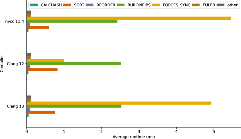
Figure 5: Average runtime (in ms) per command invocation of the largest contributors, by compiler, with the initial code.

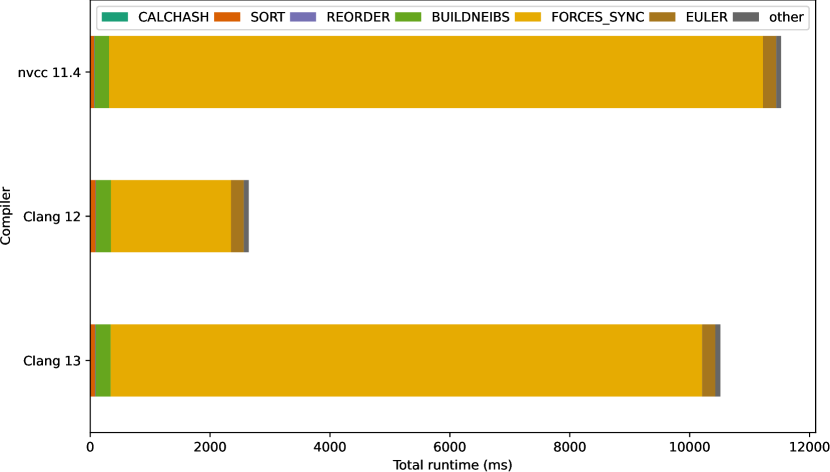
Figure 6: Total cumulative runtime (in ms) for each command during the first 1000 simulation steps of the performance analysis test-case, by compiler, with the initial code.

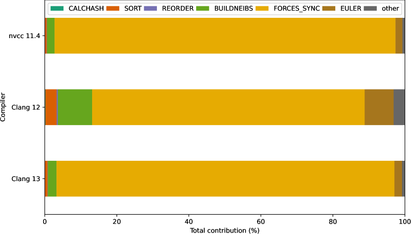
Figure 7: Percent contribution by each command to the total runtime during the first 1000 simulation steps of the performance analysis test-case, by compiler, with the initial code.

The test case used for the comparison is a three-dimensional dam-break with in a $1.6\text{m}\times 0.67\text{m}\times 0.6\text{m}$ domain. The initial water volume occupies one side of the box, up to a height and depth of $H=0.4$m. Framework options include Lennard–Jones boundary conditions for the solid walls, artificial viscosity, and the Molteni & Colagrossi [49] density diffusion model.

The simulations, consisting of $53,248$ fluid and $30,388$ boundary (for a total of $83,648$) particles at a resolution of 32 particles in the $H$ length (ppH), were only run for $1,000$ iterations, to gather basic information about total runtime and per-command contributions (Figures 5–7). Data was not saved, since we were only interested in the computational performance. The results illustrated in the plots Figures 5–7 refers to execution on an NVIDIA GeForce GTX 1650 Max-Q.

The first comparison was done between nvcc 11.4 and Clang 12. It was observed (Figures 5 and 6), that many commands had in fact a marginal performance regression with Clang, with the most significant exception being the FORCES_SYNC command that runs the forces computation kernels, that take up the lion’s share of the simulation (Figure 7), thanks also to the fact that FORCES_SYNC and EULER are run twice per time-step, while the ancillary commands for neighbors list construction (CALCHASH, SORT, REORDER, BUILDNEIBS), are only run once every 10 time-steps.

A second surprising result came with the release of Clang 13, testing on which resulted in performances within less than $20\%$ of those obtained when comping with nvcc (sometimes in excess, sometimes in defect, depending on test case and GPU architecture). Compared to the consistently improved performance of Clang 12 the results from Clang 13 were considered a regression in the compiler, and reported as an issue to the Clang developers [5].

A more thorough analysis of the forces kernels revealed that the key to the performance differences was in the usage of the stack. On GPU, use of the stack is particularly nefarious, as it involves the use of appropriately reserved global memory, which is no less than two orders of magnitude slower than registers, and can introduce significant latency in hot-path code. Two elements were in fact surprising about the stack usage reported for the forces (and many other) kernels: the first was that, since all device functions are marked with the always_inline attribute in GPUSPH, there should have been no stack usage at all; and the second was the question why Clang up to version 12 managed to avoid it, whereas the other compilers (all nvcc version and Clang 13 and higher) required it.

While the latter remains a mystery to date, resolved in Clang 14 by introducing an additional optimization pass in the compilation of CUDA code, the first question was answered by discovering the culprit in the virtual inheritance involved in the definition of the neighbors list iterators. Avoiding this was key to providing a significant performance boost across compilers.

8.2 The return of the neighbors list: multi-type iterators

The split neighbors list described in section 5.1 makes it very efficient to traverse the list of a single neighbor type. An iterator simply needs to load the beginning of the chunk and the traversal direction (based on the neighbor type), and then load each neighbor index in sequence until the end-of-list marker is encountered.

When the same interaction needs to be computed with neighbors of different types (as is the case frequently with dynamic boundary conditions), the code necessary to traverse the neighbors list is made more complex by the need to change the offset and direction of traversal when one type is finished and the other begins, but aside from that the behavior remains essentially the same.

To abstract all this from the developer, we implemented neibs_iterator class templates that take care of all the internals, and present a simple interface with methods to retrieve the current neighbor’s index, its relative position to the central particle, and finally a method to fetch the next neighbor and inform the caller when the neighbors list is completed.

The core of all the iterators is the same: a set of variables independent of the particle type, and the internal methods to fetch and decode the neighbor information from the neighbors list. These are abstracted in a dedicated neibs_iterator_core class.

All the single-type neibs_iterator class templates derive from the core class, and simply implement on top of it the necessary detail for the specific neighbor type, such as the computation of the chunk start offset and the traversal direction.

Figure 8: Diamond inheritance of base classes with and without virtual inheritance through intermediate classes. In the standard case (left), two copies of the core class are inherited by the multi-type iterator, making any reference to neibs_iterator_core ambiguous. With virtual inheritance (right), a single copy of the core class is inherited, making it possible to access neibs_iterator_core unambigious in the multi-type iterator.

The straightforward way to implement a multi-type iterator is to create a dedicated class that derives from the corresponding single-type iterators, and switches from one to the other as the end-of-list marker is reached. This however leads to the infamous diamond inheritance problem: since all the single-type iterators depend on the core class, and we want a single copy of the core class as (grand)parent of the multi-type iterator, the single-type iterators have to declare the core class as a virtual parent (Figure 8).

This virtual inheritance, however, is in our case responsible for the inefficiency experienced with nvcc and Clang 13, as the compiler fails to de-virtualize the structure. Even worse, the negative impact of the virtual inheritance affects single-type iterators too, even though for them there would be no need for virtualization in the first place: indeed, single-type iterators inherit virtually from the core class only to support multi-type iterators. This is actually in conflict with one of the principles behind the GPUSPH design, that the implementation of a feature should not negatively affect other features (in this case, the possibility to iterate over multiple types should not affect the performance of iterating over a single type).

Figure 9: Chain inheritance through nesting class templates. Single-type iterators derive directly from the core class, multi-type iterators derive from the other multi- or single-type iterators. For multi-type iterators, the order of the nesting determines the order in which neighbor types are processed. On the middle, for example, fluid types are processed before boundary types, whereas on the right boundary types are processed first.

The approach we adopted in GPUSPH to avoid virtual inheritance and its negative effects on GPU performance has been to turn multiple inheritance into chain inheritance, leveraging the fact that we iterate over neighbor types in a predefined order (Figure 9).

Instead of distinguishing between single- and multi-type iterators, we define a single class template for all iterators, with two template parameters: the particle type of the ‘current’ iterator, and the class of the ‘next’ iterator, with the template defining a class that derives from the ‘next’ iterator: this base class is then used to delegate the retrieval of the next neighbor when the current type is exhausted (Listings 16).

Listing 16: Nesting class template to implement multi-type neighbors list iterators.

⬇

template<ParticleType ptype, typename NextIterator>

class nested_neibs_iterator : public NextIterator

{

using core = neibs_iterator_core;

bool next() {

if (core::current_type == ptype) {

// fetch the next neighbor of this type

bool has_next = fetch_next_neighbor();

if (has_next) return true;

// no more neighbors: switch to next type

NextIterator::reset();

}

// this type has finished, delegate to next iterator

return NextIterator::next();

}

/* rest of the class omitted for brevity */

};

Figure 10: Average runtime (in ms) per command invocation of the largest contributors, by compiler, with the devirtualized iterators.

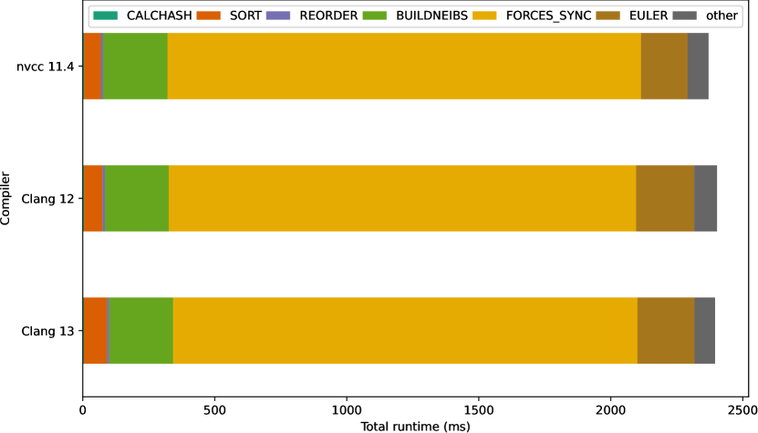
Figure 11: Total cumulative runtime (in ms) for each command during the first 1000 simulation steps of the performance analysis test-case, by compiler, with the devirtualized iterators.

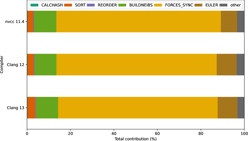
Figure 12: Percent contribution by each command to the total runtime during the first 1000 simulation steps of the performance analysis test-case, by compiler, with the devirtualized iterators.

By using the neibs_iterator_core as the “terminating” class, (i.e. the NextIterator when there are no more types to process), we ensure that all iterators inherit a single copy of it as (grand)parent through the chain, without having to resort to virtual inheritance. By adding to neibs_iterator_core a reset() method that invalidates current_type and a next() method that always returns false, the nested_neibs_iterator implements both single- and multi-type iterators with the same code, and the only distinction is given by the nesting of the classes (Figure 9).

As show in Figures 10–12, the effect of the de-virtualization of the neighbors iterator on the performances is impressive: the total runtime for nvcc and Clang 13 dropped from over 10s to less than 5s, bringing these compilers in line with the performance of Clang 12, that also benefits (although in much smaller amounts) from the optimization. Moreover, without the bottleneck created by the problematic virtual inheritance, the proprietary optimizations in nvcc allow the compiler to produce the fastest code among the ones we tested.

9 Too much of a good thing?

The impressive performance gains achieved by the rework of the neighbors traversal, that in some sense completes the split-neighbors implementation, have had some unintended consequences.

The first consequence has been an apparent decrease in the scaling efficiency of GPUSPH across multiple GPUs: this is due to the fact that high scalability relies on the forces computation taking enough time to cover the cross-device data transfer time (see [61, 60] for details): with the forces computation being much faster, the amount of inner particles that need to be processed to cover data transfers has grown significantly, thus requiring much larger domains to achieve good scaling. This of course is compensated by the fact that a single GPU now manages to perform as well as 4 or 5 GPUs used to with the older code, thereby reducing the need for multi-GPU or multi-node to very large simulations, where the amount of inner particles becomes large enough to preserve the scaling properties. Further details with examples are discussed in Section 10.3

The second consequence of the forces kernels performance gain has more of a psychological than computational weight: as shown in Figure 10, forces computation is not the slowest step of the simulation anymore: although forces computation is still the kernel where most time is spent overall (Figure 12), its runtime for a single invocation is now comparable to the runtime of the neighbors list construction.

In fact, for smaller simulations such as the one shown in this analysis, a single run of the neighbors list construction can take more time than a single forces computation, with the discrepancy growing smaller as the number of particle increases, and forces computation still taking longer (although not much so) than neighbors list construction in the case of very large simulations.

In itself this effect is not particularly worrying, since the forces kernel runs twice per step (due to the predictor/corrector integration scheme), while the neighbors list construction only runs once every 10 steps (by default). As such, even when the two have comparable runtime, forces computation still weight 20 times more than the neighbors list construction, and optimization of the latter would be largely unnecessary, since even a $50\%$ speed-up would only affect the total runtime of the simulation by less than $3\%$.

Still there is a psychological effect: knowing that building the neighbors list takes longer than a single forces computation is frustrating for a numerical code that should spend most of its time computing (numerical) derivatives. Hence the need to optimize the neighbors list construction.

9.1 Changing perspective: from the particle to the cell

As mentioned in section 2.2, WCSPH with an explicit integrator lends itself to a natural parallelization where each work-item is associated with a particle. This is also true for the neighbors list construction: each particle looks for neighbors in the cells surrounding its own (section 2.3), adding them to the neighbors list according to their type (section 5.1).

This approach is trivial to implement, but leads to poor performance due to the scattered global memory accesses and consequent large latencies as the neighbors data is fetched, with the work-items unable to proceed until the data becomes available and decisions about the neighbors (Is it close enough? Which type does it belong to? Where does it go in the list?) must be made.

The first optimization is to take advantage of the split-neighbors layout to streamline the neighbors search. As particles are sorted in memory by cell, and within the cell by particle type (and finally by particle ID), we know that whenever looking at neighbors in a cell the central particle will first see all fluid particles, then all boundary particles, etc. Instead of a single loop going over all the particles in the cell, we can thus split the code into multiple loops, one per particle type.

Listing 17: Traversing the neighbors in a cell by particle type.

⬇

template<ParticleType nptype, /* omissis */ >

void neibsInCellOfType

(params_t const& params, var_t const& var, /* omissis */)

{

/* from the neighbor loaded in var, keep processing all neighbors

* until the next loaded one is not of the same type

*/

for ( ; var.is_neib_of_type<nptype>(params); var.next_neib())

{

/* process this neighbor */

}

}

template<typename params_t, /* omissis */>

void neibsInCell(params_t const& params, /* omissis */)

{

/* omissis */

var_t vars(params, /* omissis */);

// Load information about the first neighbor

var.load_neib_info(params);

// Process neighbors by type, leveraging the fact that

// within cells they are sorted by type.

// Each instance of neibsInCellOfType will process the neighbors

// of the given type, and return when the next loaded neighbor

// (if any) is of a different type

if (var.neib_type == PT_FLUID)

neibsInCellOfType<PT_FLUID, /* omissis */>

(params, var, /* omissis */);

if (var.neib_type == PT_BOUNDARY)

neibsInCellOfType<PT_BOUNDARY, /* omissis */>

(params, var, /* omissis */);

if (boundarytype == SA_BOUNDARY && var.neib_type == PT_VERTEX)

neibsInCellOfType<PT_VERTEX, /* omissis */>

(params, var, /* omissis */);

};

Since the structure of the loop is largely the same, the loop can be implemented as a function template, parametrized on the neighbor type, taking care of all the neighbors of the given type, and returning when the next neighbor is of a differen type (or there are no more neighbors). The instances of the function can be called in sequence, following the in-cell sort order (Listing 17). This change alone has been sufficient to give a performance gain in the order of $10\%$ for the neighbors list construction, due to the reduction in divergence and to some control logic moving from runtime to compile time.

More significant improvements require a complete change in perspective. To explain how, we need to observe what happens at the hardware level during the execution of the standard implementation on GPU.

Consider two particles with consecutive indices. In many cases, they will belong to the same cell, and process neighboring cells concurrently. In fact, with the per-particle perspective adopted so far, they will process the same particles in the neighboring cells concurrently: they will load at the same time the first particle in the cell at offset $(-1,-1,-1)$, decide what to do with it, then move (at the same time) to the second particle in the same cell, etc, until the neighboring cell is exhausted, and then move to the next cell.

This is not an ideal access pattern: even assuming that the memory controller supports broadcasting (so the neighboring particle data is fetched for all work-items at the same time), the effective bandwidth is limited, since each transaction only transfers the data of a single particle, whereas the controller on GPUs is designed to transfer data from consecutive memory locations to consecutive-index work-items (which is the reason why the neighbors list is stored in interleaved format on GPU, as explained in section 5.1).

To maximize throughput, we would need work-items to transfer data corresponding to adjacent particles: for example, while the work-item for particle $i$ requests the data for the first particle from the cell at offset $(-1,-1,-1)$, the work-item from particle $i+1$ should request the data for the second particle in the cell, and so on. Of course, all work-items would then need the information from the neighboring cell particles, which have been loaded by other work-items: this data can be exchanged by storing it on fast on-chip shared memory (accessible by all the work-items in the same work-group).

To maximize the usefulness of this approach, we can switch from a particle-based perspective to a cell-based perspective, leveraging the fact that on NVIDIA GPUs work-items (a.k.a. CUDA threads) do not execute independently, but proceed in lock-step grouped in 32-wide sub-groups (a.k.a. warps).

The idea is thus to map each warp to a cell, and each work-item in the warp to a particle in the cell. This guarantees that all work-items in the same warp traverse the same neighboring cells, in lock-step. Each work-item (from the same warp) then loads one particle from the neighboring cell into the shared memory, and all work-items (in the warp) process the neighbors taking the data from the shared memory.

Compared to the naive thread-to-particle mapping, the warp-to-cell mapping is considerably more complex to implement. One of the main difficulties is that it’s not possible to do early bail-outs: even work-items that are not associated to active particles must process the neighboring cells, to ensure that all neighbors data is correctly loaded; this requires additional boolean variables to be carried around, controlling whether the work-item must also process the neighbors, or only contributes to the data retrieval.

Additionally, a cell may contain more particles than there are work-items in the warp. Therefore, both the central particle selection and the neighbor data loads are run in a “sliding window” fashion, until exhaustion of the cell particles.

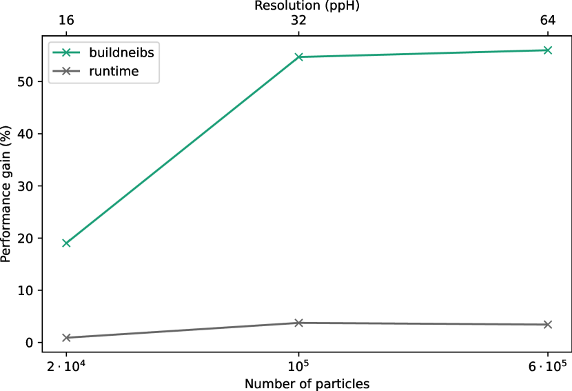
Figure 13: Performance gain (see the text for the details) in the average runtime for the neighbors list construction and in the total runtime, using the per-cell approach over the per-particle approach, with the nvcc compiler.

That being said, in the most common configuration of SPH smoothing kernels with radius $k=2$ and smoothing factors of $h=1.3$, cells in three-dimensional problems have less than 32 particles. This actually leads to a sub-optimal usage of the hardware, since every running warp will have some work-items masked out (typically, only the first 20 to 24 work-items in each warp will be active), leading to a hardware efficiency of $75\%$ or less, compared to the particle-based approach where all work-items will be active and running.

Despite this inefficiency, however, the cell mapping comes out to be around $50\%$ faster than the particle-based approach, due to the significant improvements in memory access patterns and the consequent reduction in latency. This is consistent with Volkov’s findings about the relative importance of latency and occupancy in gauging parallel algorithms and their performance on GPU [68, 69].

This performance gain (computed as the relative change in runtime, i.e. $T_{\text{old}}/T_{\text{new}}-1$, where $T_{\text{old}},T_{\text{new}}-1$ are the runtimes of the old and new code) in the neighbors list construction runtime only has a modest effect on the total runtime (Figure 13), diminishing as the number of particles grows larger.

As mentioned, this is expected, due to the lower frequency of execution of the neighbors list construction in typical simulations, but the benefits can become important if the list needs to be updated more frequently.

10 An industrial test case

The performance gains presented so far are crucial in industrial applications of SPH, for which hundreds of millions of particles are typically employed, due to large domain sizes and/or fine resolutions.

We illustrate this in a real-world test case, showing performance results including single-node and multi-node scaling performance before and after the recent optimizations, and validation of the simulation results against experimental data.

10.1 Test case setup

The test case refers to a large-scale wave maker and basin with a bounding box that is approximately $65\text{m}\times 85\text{m}$ (Figure 14). The wave is generated by a caisson system to produce a nominal maximum wave height $H=0.9$m with period $T=7.5$s. The water depth at the caisson is $d=3.4$m and decreases to $0$m at the end of the basin with a non-uniform reef bathymetry in-between.

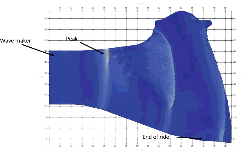
Figure 14: Overhead view of the irregularly-shaped wave basin with variable bottom bathymetry used in the test case, including the location of the three wave gages used for the comparison between the experimental and numerical data.

For the SPH simulations, the Lennard–Jones boundary model was used, with a geometric description of the basin bathymetry through a Digital Elevation Model exerting a point-wise normal Lennard–Jones force [7]. The water is assumed inviscid, and no turbulent or artificial viscosity terms are included in the momentum equation. The Molteni & Colagross density diffusion model [49] is used. The chosen SPH kernel is the Wendland quintic with radius 2, and smoothing factor 1.3.

The hardware used for the run consists of 3 nodes with 3 RTX 3090 GPUs each. Each GPU is equipped with $24$GB of GDDR6X VRAM running at $1.2$GHz wit a peak theoretical bandwidth of $936$GB/s, and $82$ compute units with $128$ shader processors each for a total of $10,496$ “CUDA cores” per GPU, with a peak theoretical throughput of around $30$TFLOPS for single-precision FMA. Due to the hardware setup, peering between GPUs within a node was unavailable, lowering the multi-GPU scaling performance, as discussed below. The nodes are equipped with 1Gbps network cards and are interconnected through a 24-port switch.

10.2 Validation

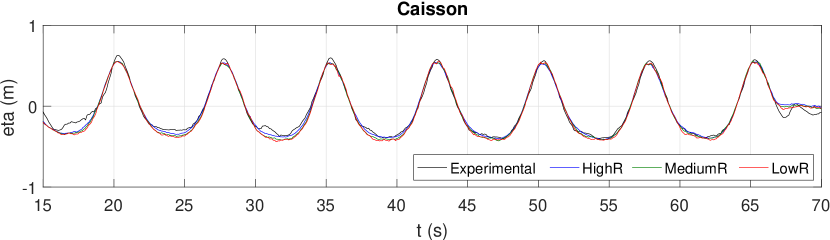
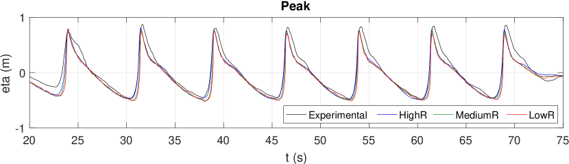
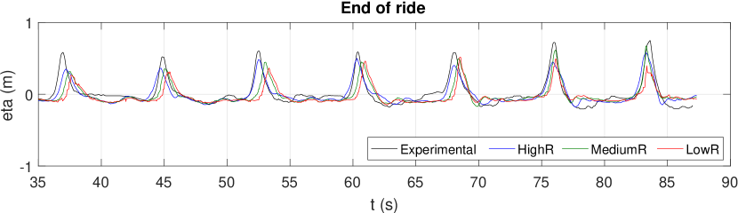
Figure 15: Water surface elevation over time from the experimental data compared with the low, medium and high resolution SPH simulations at the caisson (top figure), peak (middle figure) and end-of-ride (bottom figure).

Comparison between the physical experiments and SPH simulations were done comparing the water surface elevation and time-of-arrival at three distinct gage positions: near the caisson, where the peak wave height is expected, and at the end of the ride (Figure 15). Simulations were run at thee different resolutions, with inter-particle spacing respectively $\Delta p=0.01,0.008,0.005$m resulting respectively in (fluid $+$ boundary $=$ total) $4+2.4=6.4,7.7+3.8=11.5$ and $32+10=42$ million particles.

Even though the chosen options result in a quite simple model, the results show good accuracy. Thanks to the choice of density diffusion model, the simulation is stable over the simulated period despite the absence of viscous dissipation in the momentum equation. As expected, the match of the wave timing and crest height improve at higher resolutions. The largest discrepancy is seen at the end-of-ride gage, where excessive dissipation is observed even at higher resolutions. This effect may be reduced with the adoption of better conservation models such as the CCSPH model presented in [75], at the cost of higher computational requirements.

10.3 Performance results

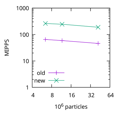
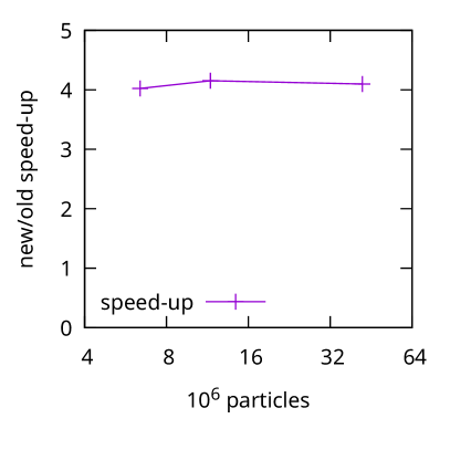
Figure 16: Single-GPU performance with the old (unoptimized) and new (optimized) neighbors list construction and traversal code. Left: performance (in MIPPS). Right: performance ratio.

Single-GPU

In our performance analysis we start by comparing the single-GPU performance across different resolutions before and after introducing the neighbors list construction and traversal optimizations. The performance is used in millions of iterations times particles per second (MIPPS), a metric we first introduced in [61]. As show in Figure 16, the performance ratio for this test case at the tested resolutions is essentially constant, with the optimizations bringing a consistent $4\times$ speed-up to the code. The decrease in MIPPS at higher resolutions is due to the higher percentage of fluid particles in the total particle count, and the higher computational requirements for fluid particles, for which the physical equations of motions have to be solved, over boundary particles, that only contribute to the forces applied to the fluid particles in their influence sphere.

Multi-GPU

We can evaluate the strong scaling capability of GPUSPH by comparing the performance of our code at given resolutions on a growing number of device. This is usually achieved by looking at the ratio $T_{1}/(nT_{n})$ where $T_{i}$ represents the runtime with $i$ devices. Using our preferred unit of measure is the number of iterations times particles per second, the scaling efficiency can be likewise measured as $P_{n}/(nP_{1})$ where $P_{i}$ is the number of MIPPS achieved with $i$ devices.

Due to the embarrassingly parallel nature of WCSPH with explicit integration —as used in our tests— the only major factor impacting scalability comes from the latency introduced between solver steps when transferring data about neighbors to/from other devices. As explained in [61, 60], each device in GPUSPH holds a copy of the data belonging to neighboring particles (“halo” particles) that reside on other device, and this is updated after each computational kernel, with the exception of the integration, which is a simple increment without any neighbors list traversal, and is therefore done on the halo particles with the forces data transferred from the neighboring devices after the forces computation kernel.

Historically, the forces computation kernel has been the most computationally expensive kernel, and this has been used to minimize the impact of data transfer on scaling performance, by first computing the forces on the particles to be transferred to other devices, and then running the computation on the rest of the domain (inner particles) while the computed forces are being copied. This allowed GPUSPH to achieve nearly ideal scaling [61, 8] under the condition that the time needed to transfer the halo particles data is less than the time needed to compute the forces on the inner particles.

This typically requires fast device-to-device transfers (e.g. through peering for devices on the same node, or solutions such as GPU Direct in multi-node configurations), and a sufficient number of inner particles. With the speed-up of the forces kernel computations coming from the optimized neighbors traversal code, we can expect the scaling performance of the new code to degrade compared to the scaling performance of the old code, especially when the number of particles (and especially inner particles) is small. The effect will be particularly evident in our tests due to the hardware configuration that prevents device peering, and even more so in the multi-node cases due to the higher latency and lower bandwidth of network data transfers compared to transfers within the same node.

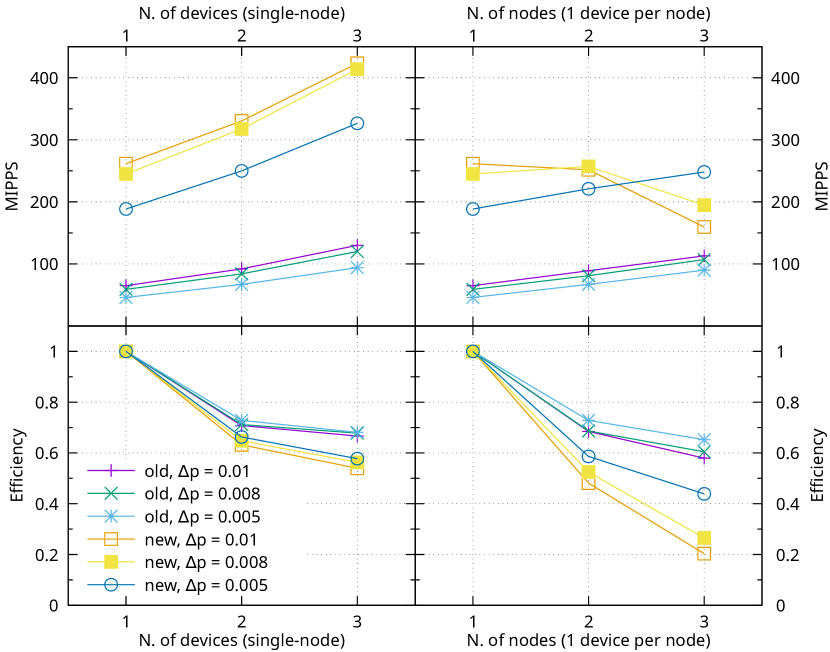
Figure 17: Performance (top) and strong scaling (bottom) at different resolutions. The left plots refer to the multi-GPU single-node case. The right plots refer to the multi-node case, with 1 GPU per node.

The results for $1$ to $3$ devices are shown in Figure 17, separating the single-node multi-GPU results (with all devices attached to the same host machine) from the multi-node results, limited in this case to 1 GPU per node.

In the single-node case, where data transfers are more efficient, all tests show performance growing with the number of GPUs. The old code has lower performance, but better scaling, with an efficiency of around $70\%$, whereas the new code drops to an efficiency as low as $53\%$ in the low resolution case ($57\%$ at the highest resolution).

This is due to the much faster forces computation kernel in the new version of the code failing to fully cover the latency introduced by the data transfer. The effect is even more evident in the multi-node, 1 GPU per node case, where the overall performance of the code actually drops as the number of nodes grows, with the only exception being the highest resolution case, where the workload for the forces computation kernel is sufficient to cover at least part of the network data transfers. Both versions of the code suffer from the more expensive data transfers, with the old code efficiency dropping to between $58\%$ (low resolution) and $65\%$ (high resolution), and the new code only managing $44\%$ efficiency at high resolution, with the low resolution dropping to $20\%$.

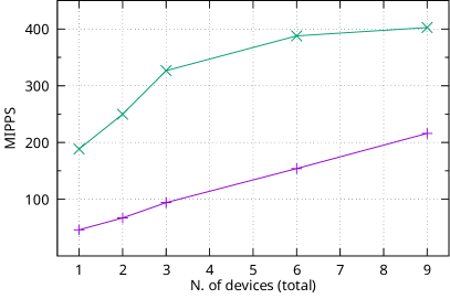
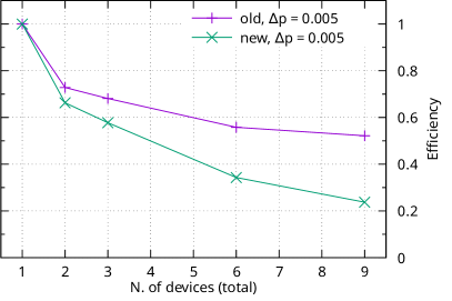
Figure 18: Performance (left) and strong scaling (right) for the high resolution case. A single node is used for up to 3 devices, with 6 and 9 devices using 2 and 3 nodes respectively.

Due to the insufficient computational load in the lower resolution cases, we only test the configuration with up to 9 devices (3 nodes with 3 devices each) in the high resolution case. The results are shown in Figure 18. Increasing the number of devices in this case always results in higher performance (and thus faster simulations), but there are diminishing returns as the number of particles assigned to each device decreases.

Once again the effect is more evident with the new, faster code, that needs a larger number of particles for the forces kernel computation to take enough time to cover the data transfers, especially in the multi-node, 3 GPUs per node configurations. Given the scaling of the forces kernel, we would expect no less than $6\times$ the number of inner particles per GPU to be needed to achieve scaling efficiency comparable to that of the old code.

11 Conclusions

The more recent revisions of the C++ language provide opportunities that can help in the design and implementation of complex code bases for scientific computing that need to support several features without loss of performance and keeping code complexity low.

Key programming patterns and C++ features such as conditional inheritance for class templates and SFINAE for function template specialization allow significant levels of code abstraction and genericity, providing at the same time several opportunities for the compiler to optimize away unnecessary variables and computations.

Helping the compiler produce better code is an effective way to speed up your program, but the final result still largely depends on the quality of the compiler, and the ability of its optimizer to leverage the opportunities offered by the developer.

On GPUs, where some programming patterns can result in excessive use of the main memory instead of hardware registers to hold temporary data, catching or missing optimization opportunities can change the performance of individual kernels by nearly an order of magnitude. As a result, the choice of the compiler can be at least as important as the coding strategies in delivering the best performance on any given hardware, although significant differences between compilers are a likely indication of “code smells”, i.e. sections of the code that are still using sub-optimal, and thus harder to optimize, patterns.

When it comes to implementations of the SPH method, and meshless methods in general, one of the crucial aspects in the performance of the code is the neighbors list: its memory layout, the way it is traversed and the way it is constructed. Careful design of the data structure and traversal methods can lead to performance gains (or losses) measurable in a factor of $3\pm 1$, especially on hardware such as GPUs that are exceptionally sensitive to register spilling and inefficient global memory usage patterns.

A paradox with the performance increase is a potential drop in the strong scaling efficiency in multi-GPU, and especially multi-node, simulations, as the shorter execution time can fail to fully cover the time necessary to transfer data between devices. This is more than compensated by the shorter computational times in general, and may imply that a much higher per-device load may be necessary to achieve comparable efficiency. Hardware setups with higher connection speed and lower latency can also help improve scaling.

The neighbors list construction itself, or in its absence the neighbors search implementation, also has a measurable impact, weighted by the frequency at which it is run. As an intrinsically memory-bound procedure, neighbors search can benefit from a change in perspective that leads to improved coalescence of memory transactions and better caching on GPU. In our experience, switching from the naive per-particle vision to an aggregate per-cell approach can lead to performance gains of as much as $50\%$ in the neighbors search despite a lower hardware occupancy. It’s possible that similar optimizations may also be possible for the main computational kernels implementing the actual numerical method, indicating that despite the appeal of SPH as an embarrassingly parallel method, optimal performance lies behind non-trivial implementation strategies.

These kinds of transformations of the numerical method into efficient code are still far from the reach of the compiler, keeping human developers still as the most effective optimizers. Despite the progress in compiler technology, there is only so much the compilers can do on their own, and it thus remains crucial for the developer to provide as much information as possible to the compiler itself, reorganizing both data structures and their access functions appropriately. The programming strategies presented in this paper, by moving as much of the control logic as possible to the compile time and by streamlining data dependencies, remain therefore essential in achieving the best performance the compiler can offer, at the cost of a less obvious mapping between the theory of the numerical method and the code implementing it, and longer development times. The latter, however, may be more than compensated by the performance gains of large simulations (frequently taking months to complete themselves) when speed-ups such as the ones obtained in our case are possible: runtimes dropping from months to weeks are definitely worth the investment in a month of developer time. Additionally, the abstractions and code strategies presented here are key elements to the implementation of heterogeneous hardware support, covering CPUs and GPUs from different vendors, as shown in the upcoming manuscript [6].

References

- Adami et al. [2012] Adami, S., Hu, X.Y., Adams, N.A., 2012. A generalized wall boundary condition for Smoothed Particle Hydrodynamics. Journal of Computational Physics 231, 7057–7075. doi:10.1016/j.jcp.2012.05.005.
- Alexandrescu [2001] Alexandrescu, A., 2001. Modern C++ Design. Addison-Wesley.
- Alexandrou et al. [2001] Alexandrou, A.N., McGilvreay, T.M., Burgos, G., 2001. Steady Herschel–Bulkley fluid flow in three-dimensional expansions. Journal of Non-Newtonian Fluid Mechanics 100, 77–96. doi:10.1016/50377-0257(01)00127-6.
- Batchelor [1974] Batchelor, G.K., 1974. An introduction to fluid mechanics. Cambridge University Press.
- [5] Bilotta, G., . Bug 52037 - performance regression in CUDA code compiled by Clang 13 versus Clang 12 (Clang 12 50% faster than Clang 13). URL: https://bugs.llvm.org/show_bug.cgi?id=52037.
- Bilotta [2023] Bilotta, G., 2023. From GPU to CPU (and beyond): extending hardware support in GPUSPH through a SYCL-inspired interface. sub judice.
- Bilotta et al. [2016] Bilotta, G., Hérault, A., Cappello, A., Ganci, G., Del Negro, C., 2016. GPUSPH: a Smoothed Particle Hydrodynamics model for the thermal and rheological evolution of lava flows, in: Detecting, Modelling and Responding to Effusive Eruptions. Geological Society of London. volume 426 of Geological Society, London, Special Publications, pp. 387–408. doi:10.1144/SP426.24.
- Bilotta et al. [2022] Bilotta, G., Zago, V., Centorrino, V., Dalrymple, R.A., Hérault, A., Del Negro, C., 2022. A numerically robust, parallel-friendly variant of BiCGSTAB for the semi-implicit integration of the viscous term in smoothed particle hydrodynamics. Journal of Computational Physics 446, 111413. URL: https://www.sciencedirect.com/science/article/pii/S0021999122004752, doi:10.1016/j.jcp.2022.111413.
- Bilotta et al. [2018] Bilotta, G., Zago, V., Hérault, A., 2018. Design and implementation of particle systems for meshfree methods with high performance, in: Chickerur, S. (Ed.), High Performance Parallel Computing. IntechOpen, Rijeka. chapter 6. URL: https://doi.org/10.5772/intechopen.81755, doi:10.5772/intechopen.81755.
- Bilotta et al. [2019] Bilotta, G., Zago, V., Hérault, A., Saikali, E., Dalrymple, R.A., 2019. Bigger, cleaner, faster: notes on the implementation of a powerful, flexible, high-performance SPH computational engine, in: Proceedings of the 14th SPHERIC Workshop, Exeter, UK.
- Bingham [1922] Bingham, E.C., 1922. Fluidity and Plasticity. McGraw-Hill, New York.
- Brezzi and Pitkäranta [1984] Brezzi, F., Pitkäranta, J., 1984. On the stabilization of finite element approximations of the Stokes equations, in: Hackbusch, W. (Ed.), Efficient Solutions of Elliptic Systems: Proceedings of a GAMM-Seminar Kiel, January 27 to 29, 1984. Vieweg+Teubner Verlag, Wiesbaden, pp. 11–19. doi:10.1007/978-3-663-14169-3\_2.
- Cavelan et al. [2020] Cavelan, A., Cabezón, R.M., Korndorfer, J.H.M., Ciorba, F.M., 2020. Finding neighbors in a forest: a -tree for smoothed particle hydrodynamics simulations. doi:10.48550/arXiv.1910.02639.
- Chen et al. [1999] Chen, J.K., Beraun, J.E., Jih, C.J., 1999. An improvement for tensile instability in Smoothed Particle Hydrodynamics. Computational Mechanics 23, 279–287. doi:10.1007/s004660050409.
- Clang Team [a] Clang Team, a. Clang: a C language family frontend for LLVM. URL: https://clang.llvm.org/.
- Clang Team [b] Clang Team, b. Compiling CUDA with clang. URL: https://llvm.org/docs/CompileCudaWithLLVM.html.
- Cleary and Monaghan [1999] Cleary, P.W., Monaghan, J.J., 1999. Conduction modelling using smoothed particle hydrodynamics. Journal of Computational Physics 148, 227 – 264. doi:10.1006/jcph.1998.6118.
- Colagrossi and Landrini [2003] Colagrossi, A., Landrini, M., 2003. Numerical simulation of interfacial flows by smoothed particle hydrodynamics. Journal of Computational Physics 191, 448–475. doi:10.1016/S0021-9991(03)00324-3.
- Cole [1948] Cole, R.H., 1948. Underwater Explosion. Princeton, NJ: Princeton University Press.
- Crespo et al. [2007] Crespo, A.J.C., Gómez-Gesteira, M., Dalrymple, R.A., 2007. Boundary conditions generated by dynamic particles in SPH methods. Computers, Materials, & Continua 5, 173–184.
- Dalrymple and Knio [2001] Dalrymple, R.A., Knio, O., 2001. SPH modelling of water waves, in: Coastal dynamics 2001, pp. 779–787.
- De Kee and Turcotte [1980] De Kee, D., Turcotte, G., 1980. Viscosity of biomaterials. Chemical Engineering Communications 6, 273–282. doi:10.1080/00986448008912535.
- Domínguez et al. [2011] Domínguez, J.M., Crespo, A.J.C., Gómez-Gesteira, M., Marongiu, J.C., 2011. Neighbour lists in smoothed particle hydrodynamics. International Journal for Numerical Methods in Fluids 67, 2026–2042. doi:10.1002/fld.2481.
- Español and Revenga [2003] Español, P., Revenga, M., 2003. Smoothed dissipative particle dynamics. Phys. Rev. E 67.
- Farhadi et al. [2018] Farhadi, A., Mayrhofer, A., Tritthart, M., Glas, M., Habersack, H., 2018. Accuracy and comparison of standard - with two variants of - turbulence models in fluvial applications. Engineering Applications of Computational Fluid Mechanics 12, 216–235. doi:10.1080/19942060.2017.1393006.
- Ferrand et al. [2017] Ferrand, M., Joly, A., Kassiotis, C., Violeau, D., Leroy, A., Morel, F.X., Rogers, B.D., 2017. Unsteady open boundaries for SPH using semi-analytical conditions and Riemann solver in 2D. Computer Physics Communications 210, 29–44. URL: http://www.sciencedirect.com/science/article/pii/S0010465516302806, doi:https://doi.org/10.1016/j.cpc.2016.09.009.
- Ferrand et al. [2012] Ferrand, M., Laurence, D.R., Rogers, B.D., Violeau, D., Kassiotis, C., 2012. Unified semi-analytical wall boundary conditions for inviscid, laminar or turbulent flows in the meshless SPH method. International Journal for Numerical Methods in Fluids 71, 446–472. URL: https://onlinelibrary.wiley.com/doi/abs/10.1002/fld.3666, doi:10.1002/fld.3666, arXiv:https://onlinelibrary.wiley.com/doi/pdf/10.1002/fld.3666.
- Ferrari et al. [2009] Ferrari, A., Dumbser, M., Toro, E.F., Armanini, A., 2009. A new 3D parallel SPH scheme for free surface flows. Computers & Fluids 38, 1203–1217. doi:10.1016/j.compfluid.2008.11.012.
- Gafton and Rosswog [2011] Gafton, E., Rosswog, S., 2011. A fast recursive coordinate bisection tree for neighbour search and gravity. Monthly Notices of the Royal Astronomical Society 418, 770–781. URL: https://doi.org/10.1111/j.1365-2966.2011.19528.x, doi:10.1111/j.1365-2966.2011.19528.x.
- Ghaïtanellis et al. [2021] Ghaïtanellis, A., Violeau, D., Liu, P.L.F., Viard, T., 2021. SPH simulation of the 2007 Chehalis Lake landslide and subsequent tsunami. Journal of Hydraulic Research 0, 1–25. URL: https://doi.org/10.1080/00221686.2020.1844814, doi:10.1080/00221686.2020.1844814, arXiv:https://doi.org/10.1080/00221686.2020.1844814.
- Gingold and Monaghan [1977] Gingold, R.A., Monaghan, J.J., 1977. Smoothed particle hydrodynamics - theory and application to non-spherical stars. Monthly Notices of the Royal Astronomical Society 181, 375–389.
- Green [2007] Green, S., 2007. Particle Simulation using CUDA. Technical Report. NVIDIA Corporation.
- Grenier et al. [2009] Grenier, N., Antuono, M., Colagrossi, A., Le Touzé, D., Alessandrini, B., 2009. An Hamiltonian interface SPH formulation for multi-fluid and free surface flows. Journal of Computational Physics 228, 8380–8393. doi:10.1016/j.jcp.2009.08.009.
- Guilcher et al. [2007] Guilcher, P.M., Ducrozet, G., Alessandrini, B., Ferrand, P., 2007. Water Wave Propagation using SPH Models. 2nd SPHERIC workshop, January 2007, Madrid, Spain .
- Harada et al. [2007] Harada, T., Koshizuka, S., Kawaguchi, Y., 2007. Smoothed particle hydrodynamics on GPUs. Computer Graphics International , 63–70.
- Hérault et al. [2010] Hérault, A., Bilotta, G., Dalrymple, R.A., 2010. SPH on GPU with CUDA. Journal of Hydraulic Research 48, 74–79.
- Hérault et al. [2014] Hérault, A., Bilotta, G., Dalrymple, R.A., 2014. Achieving the best accuracy in an SPH implementation, in: Proceedings of the 9th SPHERIC Workshop, Paris. pp. 134–139.
- Hérault et al. [2011] Hérault, A., Bilotta, G., Vicari, A., Rustico, E., Del Negro, C., 2011. Numerical simulation of lava flow using a GPU SPH model. Annals of Geophysics 54, 600–620. doi:10.4401/ag-5343.
- Hernquist and Katz [1989] Hernquist, L., Katz, N., 1989. TREESPH: a unification of SPH with the hierarchical tree method. Astrophysical Journal Suplement 70, 419. doi:10.1086/191344.
- Herschel and Bulkley [1926] Herschel, W.H., Bulkley, R., 1926. Konsistenzmessungen von gummi-benzol-losungen. Kolloid Zeitschrift 39, 291–300. doi:10.1007/BF01432034.
- Hu and Adams [2006] Hu, X.Y., Adams, N.A., 2006. A multi-phase SPH method for macroscopic and mesoscopic flows. Journal of Computational Physics 213, 844–861. doi:10.1016/j.jcp.2005.09.001.
- Jääskeläinen et al. [2015] Jääskeläinen, P., de La Lama, C.S., Schnetter, E., Raiskila, K., Takala, J., Berg, H., 2015. pocl: A performance-portable OpenCL implementation. International Journal of Parallel Programming 43, 752–785. doi:10.1007/s10766-014-0320-y.
- Lattner and Adve [2004] Lattner, C., Adve, V., 2004. LLVM: a compilation framework for lifelong program analysis & transformation, in: International Symposium on Code Generation and Optimization, 2004. CGO 2004., pp. 75–86. doi:10.1109/CGO.2004.1281665.
- Liu and Liu [2003] Liu, G.R., Liu, M.B., 2003. Smoothed Particle Hydrodynamics: A Meshfree Particle Method. World Scientific Publishing Company.
- Lucy [1977] Lucy, L.B., 1977. A numerical approach to the testing of the fission hypothesis. Astronomy Journal 82, 1013–1024.
- Marrone et al. [2011] Marrone, S., Antuono, M., Colagrossi, A., Colicchio, G., Le Touzé, D., Graziani, G., 2011. -SPH model for simulating violent impact flows. Computer Methods in Applied Mechanics and Engineering 200, 1526–1542. doi:10.1016/j.cma.2010.12.016.
- Mayrhofer et al. [2015] Mayrhofer, A., Ferrand, M., Kassiotis, C., Violeau, D., Morel, F.X., 2015. Unified semi-analytical wall boundary conditions in SPH: analytical extension to 3-D. Numerical Algorithms 68, 15–34. doi:10.1007/s11075-014-9835-y.
- Mayrhofer et al. [2013] Mayrhofer, A., Rogers, B.D., Violeau, D., Ferrand, M., 2013. Investigation of wall bounded flows using SPH and the unified semi-analytical wall boundary conditions. Computer Physics Communications 184, 2515–2527. URL: http://www.sciencedirect.com/science/article/pii/S0010465513002324, doi:https://doi.org/10.1016/j.cpc.2013.07.004.
- Molteni and Colagrossi [2009] Molteni, D., Colagrossi, A., 2009. A simple procedure to improve the pressure evaluation in hydrodynamic context using the SPH. Computer Physics Communications doi:10.1016/j.cpc.2008.12.004.
- Monaghan [2005] Monaghan, J.J., 2005. Smoothed Particle Hydrodynamics. Reports on Progress in Physics 68, 1703–1759. doi:10.1088/0034-4885/68/8/R01.
- Monaghan et al. [2005] Monaghan, J.J., Huppert, H.E., Worster, M.G., 2005. Solidification using smoothed particle hydrodynamics. Journal of Computational Physics 206, 684 – 705. doi:10.1016/j.jcp.2004.11.039.
- Monaghan and Kajtar [2009] Monaghan, J.J., Kajtar, J.B., 2009. SPH particle boundary forces for arbitrary boundaries. Computer Physics Communications 180, 1811–1820. doi:10.1016/j.cpc.2009.05.008.
- Morris et al. [1997] Morris, J.P., Fox, P.J., Zhu, Y., 1997. Modeling low reynolds number incompressible flows using SPH. Journal of Computational Physics 136, 214–226. doi:10.1006/jcph.1997.5776.
- Naroff [2007] Naroff, S., 2007. New LLVM C front-end, in: LLVM Developers’ Meeting Proceedings.
- Ostwald [1925] Ostwald, W., 1925. über die geschwindigkeitsfunktion der viskosität disperser systeme. Kolloid Zeitschrift 36, 99–117. doi:10.1007/BF01431449.
- Papanastasiou [1987] Papanastasiou, T.C., 1987. Flows of materials with yield. Journal of Rheology 31, 385–404. doi:10.1122/1.549926.
- [57] Paul, B., . The Mesa3D graphics library. URL: https://docs.mesa3d.org/.
- Pharr and Fernando [2004] Pharr, M., Fernando, R. (Eds.), 2004. GPU gems 2: programming techniques for high-performance graphics and general-purpose computation. Addison-Wesley.
- Rogers and Dalrymple [2005] Rogers, B.D., Dalrymple, R.A., 2005. Three-dimensional SPH-SPS modeling of wave breaking, in: Symposium on Ocean Wave Measurements and Analysis (ASCE), Madrid.
- Rustico et al. [2014a] Rustico, E., Bilotta, G., Hérault, A., Del Negro, C., Gallo, G., 2014a. Advances in multi-GPU smoothed particle hydrodynamics simulations. IEEE Transactions on Parallel and Distributed Systems 25, 43–52. doi:http://doi.ieeecomputersociety.org/10.1109/TPDS.2012.340.
- Rustico et al. [2014b] Rustico, E., Jankowski, J.A., Hérault, A., Bilotta, G., Del Negro, C., 2014b. Multi-GPU, multi-node SPH implementation with arbitrary domain decomposition, in: Proceedings of the 9th SPHERIC Workshop, Paris. pp. 127–133.
- Saffer [2010] Saffer, D., 2010. Designing for Interaction: Creating Innovative Applications and Devices. Voices That Matter, Pearson Education (US).
- Saikali et al. [2020] Saikali, E., Bilotta, G., Hérault, A., Zago, V., 2020. Accuracy improvements for single precision implementations of the SPH method. International Journal of Computational Fluid Dynamics 34, 774–787. URL: https://doi.org/10.1080/10618562.2020.1836357, doi:10.1080/10618562.2020.1836357, arXiv:https://doi.org/10.1080/10618562.2020.1836357.
- Schulze et al. [2022] Schulze, L.J., Zago, V., Bilotta, G., Dalrymple, R.A., 2022. Localized kernel gradient correction for SPH simulations of water wave propagation, in: Proceedings of the 16th SPHERIC Workshop, Catania.
- Stroustrup [2014] Stroustrup, B., 2014. Programming: Principles and Practice Using C++. 2nd ed., Addison–Wesley.
- Toit [2011] Toit, S.D. (Ed.), 2011. ISO/IEC 14882:2011 Information technology — Programming languages — C++. 3 ed., International Organization for Standardization.
- Vila [1999] Vila, J.P., 1999. On particle weighted methods and smooth particle hydrodynamics. Mathematical Models and Methods in Applied Sciences 9. doi:10.1142/S0218202599000117.
- Volkov [2010] Volkov, V., 2010. Better performance at lower occupancy, in: Proceedings of the GPU Technology Conference 10.
- Volkov [2016] Volkov, V., 2016. Understanding Latency Hiding on GPUs. Ph.D. thesis. EECS Department, University of California, Berkeley.
- Wu et al. [2016] Wu, J., Belevich, A., Bendersky, E., Heffernan, M., Leary, C., Pienaar, J., Roune, B., Springer, R., Weng, X., Hundt, R., 2016. Gpucc: An open-source GPGPU compiler, in: Proceedings of the 2016 International Symposium on Code Generation and Optimization, Association for Computing Machinery, New York, NY, USA. p. 105–116. URL: https://doi.org/10.1145/2854038.2854041, doi:10.1145/2854038.2854041.
- Zago et al. [2022] Zago, V., Almashan, N., Dalrymple, R.A., Bilotta, G., Al-Houti, D.B., Neelamani, S., 2022. Validation of an SPH-FEM model for offshore structure, in: Proceedings of the 16th SPHERIC Workshop, Catania.
- Zago et al. [2017] Zago, V., Bilotta, G., Cappello, A., Dalrymple, R.A., Fortuna, L., Ganci, G., Hérault, A., Del Negro, C., 2017. Simulating complex fluids with Smoothed Particle Hydrodynamics. Annals of Geophysics 60, PH669. doi:10.4401/ag-7362.
- Zago et al. [2019] Zago, V., Bilotta, G., Cappello, A., Dalrymple, R.A., Fortuna, L., Ganci, G., Hérault, A., Del Negro, C., 2019. Preliminary validation of lava benchmark tests on the GPUSPH particle engine. Annals of Geophysics 62. doi:10.4401/ag-7870.
- Zago et al. [2018] Zago, V., Bilotta, G., Hérault, A., Dalrymple, R.A., Fortuna, L., Cappello, A., Ganci, G., Del Negro, C., 2018. Semi-implicit 3D SPH on GPU for lava flows. Journal of Computational Physics 375, 854–870. doi:10.1016/j.jcp.2018.07.060.
- Zago et al. [2021] Zago, V., Schulze, L.J., Bilotta, G.A., Dalrymple, R.A., 2021. Overcoming excessive numerical dissipation in SPH modeling of water waves. Coastal Engineering 170, 104018. URL: https://www.sciencedirect.com/science/article/pii/S0378383921001666, doi:10.1016/j.coastaleng.2021.104018.
- Zeller [2007] Zeller, C. (Ed.), 2007. NVIDIA CUDA Programming Guide, Version 1.0. NVIDIA Corporation.
- Zhu et al. [2005] Zhu, H., Kim, Y.D., De Kee, D., 2005. Non-newtonian fluids with a yield stress. Journal of Non-Newtonian Fluid Mechanics 129, 177–181. doi:10.1016/j.jnnfm.2005.06.001.